


Introduction
Artificial engineered materials exhibiting extraordinary and unconventional electromagnetic properties at microwave and optical frequencies are more and more involved in research activities as well as in application scenarios. These materials allow one to attain unusual performance not available in nature, thus overcoming some limitations due to the use of natural materials and designing an amazing artificial world from the electromagnetic point of view. Metamaterials (MTMs) denote a very attractive class of artificial materials that can be obtained by embedding small inclusions in host media or by connecting inhomogeneities to host surfaces. Definitions, properties, and applications as well as useful references can be found in [Reference Bilotti and Sevgi1]. The most known MTM sub-class contains materials possessing negative real parts of permittivity and permeability, and therefore they are referred to as double-negative metamaterials (DNG MTMs). Accordingly, the solution of diffraction problems involving them is very appealing from theoretical and application viewpoints.
The Uniform Asymptotic Physical Optics (UAPO) approach has recently emerged as a useful, reliable, and alternative high-frequency analytical method to obtain approximate uniform solutions to plane wave diffraction problems involving penetrable and impenetrable structures [Reference Gennarelli, Pelosi, Pochini and Riccio2–Reference Frongillo, Gennarelli and Riccio19]. The UAPO solutions can be used in the framework of the Uniform Geometrical Theory of Diffraction (UTD) [Reference Kouyoumjian and Pathak20] and are expressed in a closed form containing only standard functions and parameters as the trigonometric functions, the UTD transition function, and the geometrical optics (GO) response of the structure in terms of reflection and transmission coefficients.
The UAPO approach was previously applied to a lossy DNG MTM slab [Reference Gennarelli and Riccio10] to obtain total field values by adding GO and UAPO field data. Numerical tests confirmed the ability of the UAPO diffracted field to compensate the jumps of the GO field at the shadow boundaries and to produce a total field in good agreement with the output of a well-known commercial solver. Such results suggest the utilization of the UAPO approach in order to solve the plane wave diffraction problem involving a planar junction formed by a lossy DNG MTM slab and a thick flat metal. A key point of the analytical evaluation process is related to the linearity of the radiation integral. This allows one to obtain the UAPO solution relevant to the planar structure by combining the UAPO contributions of the two slabs.
The diffraction problem involving a junction between two half-planes with different boundary conditions has been tackled and solved in literature by means of many techniques (see [Reference Gennarelli, Pelosi, Riccio and Toso3, Reference Uzgoren, Buyukasoy and Serbest21–Reference Umul29] for a short and non-exhaustive list of reference). A DNG MTM sheet together with a metallic one forms a very interesting structure for the design of innovative antenna systems as well as for the control and manipulation of the propagation of electromagnetic, optical, and acoustic waves in advanced devices.
The manuscript is organized as follows. Section “The UAPO diffracted field” contains the application of the UAPO approach to the evaluation of the diffracted field by the considered structure when a plane wave impinges at skew incidence with respect to the rectilinear discontinuity of the junction (see Fig. 1). The resulting formula is UTD-like and its efficiency is tested in section “Numerical tests” by means of numerical simulations. Highlights and comments are collected in section “Conclusions”.

Fig. 1. The diffraction problem.
The UAPO diffracted field
The geometry of the diffraction problem is shown in Fig. 1, where the z-axis of the co-ordinate reference system is chosen to be coincident with the rectilinear discontinuity of the junction, which is surrounded by the free space. The flat metal changes in a perfect electrically conducting (PEC) half-plane and the DNG MTM slab is modeled by a penetrable half-plane, which is characterized by the thickness d, the relative electric permittivity $\varepsilon _r = {-}\varepsilon ^{\prime}-j\varepsilon$ ", and the relative magnetic permeability $\mu _r = {-}\mu ^{\prime}-j\mu$
 ".
".
In the UTD framework, the diffracted electric field $\underline E ^d$ in the ray-fixed reference system $\hat{\beta }\comma \;\hat{\phi }$
 is associated with the incident field $\underline E ^i$
 in the ray-fixed reference system $\hat{\beta }^{\prime}\comma \;\hat{\phi }^{\prime}$
 by the well-known formula:

where $\underline{\underline D}$ is the diffraction matrix, s is the distance from the diffraction point to the observation point P, and k 0 is the free-space propagation constant. This section is devoted to the UAPO formulation of $\underline{\underline D}$
 for the considered junction.
The application of the UAPO approach to penetrable half-planes is based on PO equivalent sources that match the half-plane surface and radiate in the free space. Consequently, the scattered field $\underline E ^s$ due to the considered PO sources can be so expressed:

where ζ 0 is the free-space impedance, r is the position vector of P, $\underline{r} ^{\prime} = x^{\prime}\hat{x} + z^{\prime}\hat{z}$ denotes the source points on the surfaces S DNG and S PEC, $\hat{R} = {{\lpar \underline r -\underline r ^{\prime}\rpar } / {\vert {\underline r -\underline r^{\prime}} \vert }}$
 , the symbol “${\wedge}$
 ” indicates the cross product, and $\underline{\underline I}$
 is the 3 × 3 identity matrix. The sources $\underline{J} {\kern 1pt} _s^{DNG}$
 and $\underline{J} {\kern 1pt} _{ms}^{DNG}$
 are the electric and magnetic PO equivalent surface currents associated with the DNG MTM half-plane. If $\hat{s}^{\prime} = {-}\sin \beta ^{\prime}\cos \phi ^{\prime}\hat{x}-\sin \beta ^{\prime}\sin \phi ^{\prime}\hat{y} + \cos \beta ^{\prime}\hat{z}$
 is the unit vector of the incidence direction (see Fig. 1), $\hat{e}_\bot$
 is the unit vector perpendicular to the incidence plane and $\vartheta ^i$
 is the standard incidence angle, it results:


where the reflection (Γ) and transmission (τ) coefficients for parallel $\lpar \,\parallel \,\rpar$ and perpendicular (⊥) polarizations are determined according to [Reference Gennarelli and Riccio10]. The PO surface current $\underline{J} {\kern 1pt} _s^{PEC}$
 on the lit face of the PEC half-plane is given by:

The next approximation in the UAPO approach is $\hat{R}\cong \hat{s} = \sin \beta \cos \phi \,\hat{x} + \sin \beta \sin \phi \,\hat{y} + \cos \beta \,\hat{z}$ ($\hat{s}$
 denotes the diffraction direction on the Keller's cone with β = β ′). This allows one to rewrite the formula (2) as:

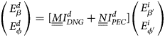
The above expression can be now arranged in matrix form to evaluate the components $E_\beta ^s$ and $E_\phi ^s$
 in terms of $E_{\beta ^{\prime}}^i$
 and $E_{\phi ^{\prime}}^i$
 according to (1):

where


The matrices in (8) and (9) are reported in Appendix.
The integrals I DNG and I PEC can be analytically manipulated to obtain the UAPO diffraction matrix. The corresponding steps follow. With reference to I DNG, it is expressed by:

wherein $\vert {\underline \rho -\underline \rho^{\prime}} \vert ^2 = \lpar x-x^{\prime}\rpar ^2 + y^2$ . The z ′ integration furnishes:

A useful integral representation of the zeroth-order Hankel function of second kind $H_0^{\lpar 2\rpar } \lpar {\cdot} \rpar$ and the application of the Sommerfeld–Maliuzhinets inversion formula provide:

where C is a proper integration path in the complex α − plane. The integral in formula (12) can be evaluated by means of the steepest descent method accounting for the Cauchy residue theorem and the integral along the steepest descent path. The application of the multiplicative method and the successive asymptotic evaluation of the resulting integral permit to determine the diffraction term $I_{DNG}^d$ :
:
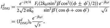
where F t( ⋅ ) denotes the UTD transition function [Reference Kouyoumjian and Pathak20]. The sign + (−) applies when 0 < ϕ < π(π < ϕ < 2π).
The diffraction term $I_{PEC}^d$ is obtained from I PEC according to the above analytical process:

At the end of the procedure, the UAPO diffracted field can be so expressed:
and the UAPO formulation of $\underline{\underline D}$ is then determined by comparing (1) and (15), i.e.

Numerical tests
This section concerns the validation of the UAPO solution for the plane wave diffraction by the considered junction. At first, the ability to compensate the GO discontinuities has been tested and then the RF module of COMSOL MULTIPHYSICS® has been used to investigate the accuracy of the total field levels. All the reported results refer to the same structure that is characterized by d = 0.25λ 0 if λ 0 is the free-space wavelength, ɛr = −2 − j0.7 and μ r = −1 − j0.5. Moreover, the incident electric field is assumed to have only the β ′ −component and the observation domain is a circular path with radius ρ = λ 0.
The β − component amplitudes of the GO and UAPO diffracted fields when (β ′ = 45°, ϕ ′ = 60°) are displayed in Fig. 2. As expected, the GO field jumps at the reflection (ϕ = 120°) and transmission shadow boundaries (ϕ = 240°). The UAPO diffracted field possesses two peaks corresponding to such directions and provides the continuity of the total field across them (see Fig. 3). This ability is also confirmed by the results in Figs 4 and 5. They are relevant to (β ′ = 60°, ϕ ′ = 125°) and assess the effectiveness of the UAPO solution in the UTD framework.

Fig. 2. The GO and UAPO diffracted fields when (β ′ = 45°, ϕ ′ = 60°).

Fig. 3. The total field when (β ′ = 45°, ϕ ′ = 60°).

Fig. 4. The GO and UAPO diffracted fields when (β ′ = 60°, ϕ ′ = 125°).

Fig. 5. The total field when (β ′ = 60°, ϕ ′ = 125°).
The accuracy of the UAPO solution in the case of an isolated DNG MTM half-plane has been proved in [Reference Gennarelli and Riccio10] by means of the RF module of COMSOL MULTIPHYSICS®. What happens with the presence of the PEC half-plane in the junction? The last set of figures (Figs 6–9) is reported to answer this question. The incidence direction is assumed orthogonal to the discontinuity as in [Reference Gennarelli and Riccio10] and the results are shown for increasing values of ϕ ′. Figure 6 refers to ϕ ′ = 30° and a very good agreement is obtained by comparing the COMSOL MULTIPHYSICS® data and the UAPO-based results in the range 0 < ϕ < 180°. A good agreement is again evident when the observation point moves in the bottom half-space. This behavior is also manifest when ϕ ′ = 60° (see Fig. 7). The successive figures are relevant to ϕ ′ > 90°. The comparisons in Fig. 8 (ϕ ′ = 110°) and Fig. 9 (ϕ ′ = 130°) show again a very good agreement in the upper half-space and in the angular region from the DNG MTM half-plane to the transmission boundary, but the performance changes when approaching the PEC half-plane. As it can be seen, the UAPO solution underestimates the field values in the shadow region of the GO field below the PEC half-plane. This result is expected according to the PO approximation for the PEC structure and highlights a limitation of the proposed solution that is efficient and manageable, but it is still an approximate solution.

Fig. 6. The β− component of the total field when (β ′ = 90°, ϕ ′ = 30°).

Fig. 7. The β− component of the total field when (β ′ = 90°, ϕ ′ = 60°).

Fig. 8. The β− component of the total field when (β ′ = 90°, ϕ ′ = 110°).

Fig. 9. The β− component of the total field when (β ′ = 90°, ϕ ′ = 130°).
Conclusions
The plane wave diffraction by a metallic–DNG MTM planar junction has been considered in this paper and a UAPO solution has been proposed in the UTD framework. The UAPO formulation of the diffraction matrix is the result of an analytical procedure, which does not require the evaluation of differential/integral equations or special functions, and provides a closed-form and easy to handle solution. The corresponding diffracted field is able to guarantee the continuity of the total field across the shadow boundaries of the GO field. Moreover, comparisons with the COMSOL MULTIPHYSICS® data confirm the effectiveness of the UAPO solution with respect to the accuracy. However, the end user must always take into account that the solution is based on the PO approximation and its limitations.
Appendix
The matrices that are involved in (8) and (9) to obtain $\underline{\underline M}$ and $\underline{\underline N}$
 are reported as follows:


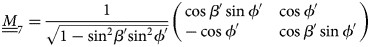


Note that $\underline{\underline M} _5$ and $\underline{\underline N} _5$
 account for the expressions of $\underline{J} {\kern 1pt} _s^{DNG}$
 and $\underline{J} {\kern 1pt} _s^{PEC}$
 , whereas $\underline{J} {\kern 1pt} _{ms}^{DNG}$
 is included in $\underline{\underline M} _6$
 .
.
 Gianluca Gennarelli received the M.Sc. degree (summa cum laude) in Electronic Engineering and the Ph.D. degree in Information Engineering at the University of Salerno, Fisciano (SA), Italy, in 2006 and 2010, respectively. He held a Post-Doctoral Fellowship at the University of Salerno from April 2010 to December 2011. Since January 2012, he has been a Research Scientist at the Institute for Electromagnetic Sensing of the Environment of the Italian National Research Council (IREA-CNR), Naples, Italy. In 2015, he has been a Visiting Scientist at the North Atlantic Treaty Organization (NATO) Science & Technology Organization (STO) Centre for Maritime Research and Experimentation (CMRE), La Spezia, Italy. His research interests cover theoretical and applied electromagnetic topics such as microwave sensors, antennas, electromagnetic inverse scattering problems, radar imaging, diffraction problems, near-field–far-field transformation techniques, and electromagnetic simulation. Dr. Gennarelli has co-authored over a hundred publications in international peer-reviewed journals and conference proceedings.
 Giovanni Riccio received the Laurea degree in Electronic Engineering from the University of Salerno, Italy. From 1995 to 2001, he was an Assistant Professor at the Engineering Faculty of the University of Salerno, where he is currently an Associate Professor of Electromagnetics. His research activity concerns non-redundant sampling representations of electromagnetic fields, near-field–far-field transformation techniques, radar cross-section of corner reflectors, wave scattering from penetrable and impenetrable structures. Giovanni Riccio is the co-author of over 250 scientific papers, mainly in international journals and conference proceedings. He is a Member of the IEEE Society and Fellow of the Electromagnetics Academy.


 Open access