


1. Introduction
The study of jump-diffusion option pricing models can be dated back to Nobel laureate Robert C. Merton's seminal paper in 1976. There have been a few extensions in the recent decades on the distributions of jump sizes (see [Reference Amin1,Reference Cai and Kou3,Reference Gukhal7,Reference Kuo8,Reference Kuo and Wang10] for some specific examples and see [Reference Cont and Tankov5,Reference Kuo9] for a review on the category of jump-diffusion models). Among the competing models, Kou's extension (see the original paper of [Reference Kuo8]) is considered to be the most representative version and has now become a new standard in the category. In such a model, the jump size is assumed to follow a double-exponential (DE) distribution which captures the tail-fatness of jump size distribution. For the convenience of our presentation, this jump-diffusion model is termed DEJD which stands for double-exponential jump-diffusion. Under the independent and identically distributed (i.i.d.) assumption on the sizes of a series of jumps, the European option price under the DEJD model can be derived in closed-form.
In this paper, we intend to relax the i.i.d. assumption in the DEJD model in order to capture the varying severity of upcoming jumps. Each jump size is still assumed to follow a DE distribution but the parameters of the distribution may change in a series of jumps. The proposed model is termed nonhomogeneous double-exponential jump-diffusion or NDEJD to reflect its nonhomogeneous nature in its parameters. While our extended model allows for each jump size to take different parameters, we focus our discussion on two particular scenarios, where (a) these jumps have growing effects and (b) they have diminishing effects. The severity is modeled by the tail-fatness of the DE distributions, meaning that the tails are getting fatter in the former scenario and getting lighter in the latter scenario. The financial implications of the two scenarios are that the impacts on stock price from a particular event can get stronger or fade away when subsequent jumps happen.
The global COVID-19 pandemic in 2020 provides us with a good opportunity to observe the growing and diminishing effects from jumps. Since the WHO (World Health Organization) declared its outbreak in March 2020, the high volatilities we witnessed in the stock markets across the globe have been unprecedented, with all major indexes fluctuating to an extreme extent that was never seen before. Plot (a) of Figure 1 shows the time series of daily log returns of VIX index from February to March 2020. It is observed that, since the crisis began, the VIX return started to surge to the first high point A (February 24), reflecting a highly uncertain prospect for the economic situation. But the effects seemed to be decreasing in the following week till point C (March 3), indicating that the market started to stabilize. In this period of time, if we treat the marked high points when the jumps happened (a surge in VIX usually indicates a big drop in the underlying S&P 500 index), namely, the three high points A, B, and C, we will clearly observe a diminishing effect which showed itself in the series of jumps.
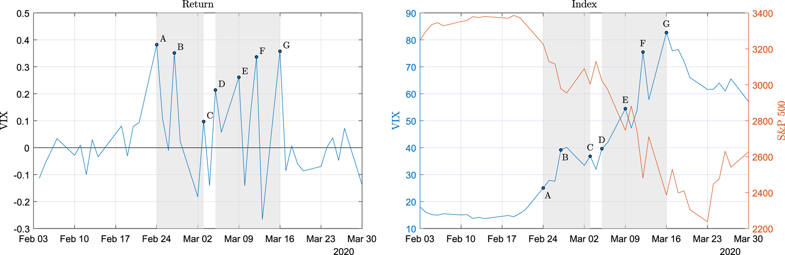
Figure 1. The growing and diminishing effects of jumps indicated by the log return (percentage change) of the VIX series over the COVID-19 pandemic period: (a) the log return of VIX and (b) the levels of VIX and S&P 500 indexes. The dates of the high points A, B, C, D, E, F, and G in the VIX returns (interpreted as jumps in the underlying S&P 500 index) are February 24 and 27, March 3, 5, 9, 12, and 16 in year 2020.
We next turn our focus to the period between points D and G (from March 5 to March 16), during which we see that there were four high points D, E, F, and G, which we identify as jumps. The increasing trend of these high VIX returns indicates that the effects of the jumps in the underlying S&P 500 index are getting stronger, reflecting an even more uncertain market situation ahead. Plot (b) of Figure 1 shows how the levels of VIX and the S&P 500 indexes were moving over the whole range of time. It is clear that in the first shaded period, the S&P 500 index plummeted, with a short downward trend which quickly ceased to continue. As a contrast, in the second shaded period, the S&P 500 index continued to drop in a stronger way since the first plunge on March 5. The observations above provide us with empirical support for our extended model, which incorporates growing or diminishing effects in a series of jumps.
In this paper, we provide a mathematical analysis for the proposed NDEJD model. As we relax the i.i.d. assumption on which most of the existing models are built, this also poses a challenge in our mathematical treatment. Using the fact that exponential distributions with different parameters sum to a hypoexponential (HE) distribution, we define a number of distributions that are closely related to HE distribution to facilitate our analysis. With the aid from these newly developed distributions, we are able to characterize the risk-neutral distribution of the stock return, based on which the European option pricing formula is derived in closed-form.
The proposed NDEJD model adds flexibility to the DEJD model and widens the coverage of market scenarios without losing mathematical tractability. Using the analytical results, we provide numerical examples that enable us to study the effects from nonhomogeneous jump sizes. We focus on the above-mentioned two scenarios where the successive jump sizes are getting fatter- or thinner-tailed reflecting the growing or diminishing effects in jumps. A comprehensive comparison is provided across these cases of interest with the DEJD model taken as a benchmark. What we will examine include: the risk-neutral distribution of stock returns, the option prices, and the bias relative to the benchmark case in them, as well as the richness in the shapes of the implied volatility smiles. Through the numerical examples provided in our analysis, we demonstrate the benefits of our extended NDEJD model relative to the original DEJD model.
The rest of this paper is structured as follows. Section 2 introduces the proposed extension of the DEJD model. Section 3 provides an analysis of the jump accumulation process under the proposed model. Section 4 further provides an analysis of stock return and European option prices. Section 5 provides numerical examples to demonstrate the influences from nonhomogeneous jump sizes. Finally, this study is concluded in Section 6.
2. The proposed model
Consider a standard jump-diffusion model for the stock price  $S_t$:
 \begin{equation} \frac{dS_t}{S_t} = \mu \,dt + \sigma \,dW_t + dJ_t,\end{equation}
where  $\mu$ is the drift coefficient, $W_t$ is a Wiener (diffusion) process, and $J_t$ is a jump process. When a jump happens at $\tau _j, j=1,2,\ldots$, the stock price will move from $S_j$ (before jump) to $S_jY_j$ (after jump). The instantaneous stock return caused by jump is $\ln (S_j Y_j/S_j) = \ln Y_j$, which is referred to as jump size in this paper. In the mainstream models such as [Reference Amin1,Reference Kuo8,Reference Merton11], the series of jump sizes $\{\ln Y_j, j=1,2,\ldots \}$ are i.i.d., and the models differ in their assumptions on the jump size distributions. In Merton's classical model [Reference Merton11], normal distribution is assumed. In Amin's extended model [Reference Amin1], bivariate distribution is assumed. Kou's DEJD model [Reference Kuo8] takes one step further to assume DE distribution. These models are mathematically tractable due to the i.i.d. property and their distributional assumptions, under which the European option prices can be derived analytically.
The purpose of this paper is to relax the i.i.d. assumption to incorporate nonhomogeneity in a series of jump sizes. We consider an extension from the DEJD model in [Reference Kuo8] because the DE assumption has gained popularity in recent decades as it successfully captures the tail-fatness of jump sizes. It should be noted that, in Merton's classical model, where normally distributed jump sizes are assumed, nonhomogeneity would not cause a problem for the mathematical analysis because normal distributions with different parameters still sum to a normal distribution. However, there will be some technical issues in the extension of DEJD model because exponential distributions with different parameters would no longer sum to an Erlang distribution.
In the DEJD model, the jump size is assumed to follow a double exponential distribution which is denoted by  $\ln Y_j\sim \mathsf {DE}(p,\eta,\tilde {\eta })$ and defined as follows:
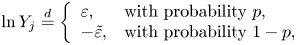 \begin{equation} \ln Y_j \stackrel{d}{=} \left\{\begin{array}{ll} \varepsilon, & \text{with probability}\ p, \\ -\tilde{\varepsilon}, & \text{with probability}\ 1-p, \end{array}\right. \end{equation}
where  $\varepsilon \sim \mathsf {Exp}(\eta )$ and $\tilde {\varepsilon }\sim \mathsf {Exp}(\tilde {\eta })$ are exponential random variables with respective means $1/\eta$ and $1/\tilde {\eta }$. As depicted in Figure 2, a DE distribution is a mixture of a positive and a negative exponential distributions, which are used to model the effect from either a positive or a negative shock caused by an unexpected jump event. In our proposed NDEJD (nonhomogeneous DEJD) model, the exponential parameters $\eta$ and $\tilde {\eta }$ are nonhomogeneous, that is, they are different from jump to jump. Specifically, we assume
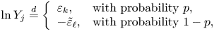 \begin{equation} \ln Y_j \stackrel{d}{=} \left\{\begin{array}{ll} \varepsilon_k, & \text{with probability}\ p, \\ -\tilde{\varepsilon}_{\ell}, & \text{with probability}\ 1-p, \end{array}\right. \end{equation}
where  $\varepsilon _k \sim \mathsf {Exp}(\eta _k)$ and $\tilde {\varepsilon }_{\ell } \sim \mathsf {Exp}(\tilde {\eta }_{\ell })$. This means that the $j$th jump is either the $k$th positive jump or the $\ell$th negative jump. (Here, $j$ is the index of all jumps, whereas $k$ and $\ell$ are respectively the indexes of positive and negative jumps.) As illustrated in Figure 3, $\{\eta _k, k=1,2,\ldots \}$ denotes the series of parameters of positive jump sizes and $\{\tilde {\eta }_{\ell }, \ell =1,2,\ldots \}$ denotes the series of parameters of negative jump sizes.
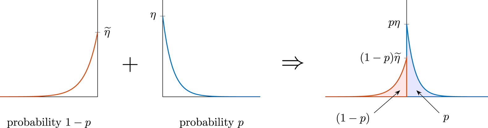
Figure 2. The double-exponential distribution in the DEJD model.
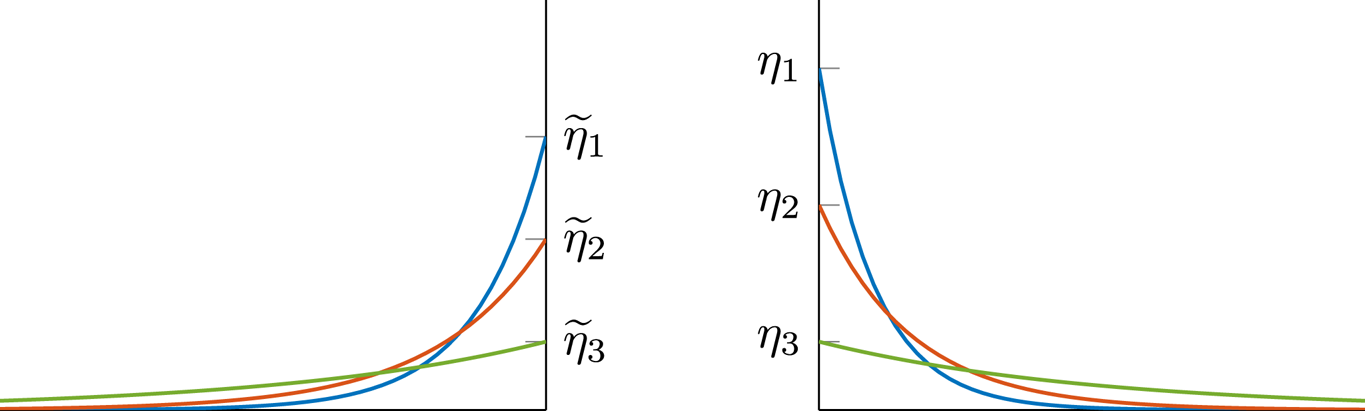
Figure 3. Nonhomogeneity in the exponentially distributed jump sizes.
In such a setting, before the occurrence of the  $j$th jump, the foregoing $j-1$ jumps include $k-1$ positive jumps and $\ell -1$ negative jumps, where $j-1 = (k-1) + (\ell -1)$. Below we give an example to illustrate our model specification. Suppose that $j-1 = 9$ jumps have already happened and their details are given as below:
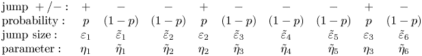 \begin{equation}\begin{array}{lccccccccc} \text{jump}\ +{/}- : & + & - & - & + & - & - & - & + & - \\ \text{probability} : & p & (1-p) & (1-p) & p & (1-p) & (1-p) & (1-p) & p & (1-p) \\ \text{jump size} : & \varepsilon_1 & \tilde{\varepsilon}_1 & \tilde{\varepsilon}_2 & \varepsilon_2 & \tilde{\varepsilon}_3 & \tilde{\varepsilon}_4 & \tilde{\varepsilon}_5 & \varepsilon_3 & \tilde{\varepsilon}_6\\ \text{parameter} : & \eta_1 & \tilde{\eta}_1 & \tilde{\eta}_2 & \eta_2 & \tilde{\eta}_3 & \tilde{\eta}_4 & \tilde{\eta}_5 & \eta_3 & \tilde{\eta}_6 \\ \end{array}\end{equation}
In the foregoing nine jumps, there are three positive and six negative jumps. The forthcoming jump is the 10th jump, and we have  $j=10$, $k = 4$, $\ell = 7$. In this case, our model assumes that $\ln Y_{10}\sim \mathsf {Exp}(\eta _4)$ with probability $p$ and $\ln Y_{10}\sim \mathsf {Exp}(\tilde {\eta }_7)$ with probability $1-p$.
For each given  $j$ (the index of the forthcoming jump), there may be different combinations of positive and negative jumps that have already happened. Therefore,
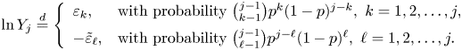 \begin{equation} \ln Y_j \stackrel{d}{=} \left\{\begin{array}{ll} \varepsilon_k, & \text{with probability}\ \binom{j-1}{k-1} p^k(1-p)^{j-k}, \ k = 1,2,\ldots,j, \\[5pt] -\tilde{\varepsilon}_\ell, & \text{with probability} \ \binom{j-1}{\ell-1} p^{j-\ell}(1-p)^\ell, \ \ell = 1,2,\ldots,j. \end{array}\right. \end{equation}
The difference between (2.3) and (2.4) is that (2.3) is conditional on knowing that  $k-1$ positive and $\ell -1$ negative jumps have already happened but (2.4) is its unconditional version without the information about the precise values of $k$ and $\ell$.
It should be noted that when nonhomogeneity is assumed for these  $\eta _k$ and $\tilde {\eta }_{\ell }$, one can not specify an infinitely large number of different values for these nonhomogeneous parameters. As will be seen, if the number of the constituent exponential distributions is too large, in theory, they still sum to a HE distribution, but in practice, the resultant HE distribution will become unmanageable (its density function is computationally infeasible). To avoid this difficulty, we assume that the Poisson process may generate at most $n^\ast$ jumps and will be stopped afterwards. By so doing, we may ease the problem in that we only need to handle (compute the distribution of) the sum of at most $n^\ast$ exponential random variables.
Under the above assumption, our Poisson process is essentially a stopped Poisson (SP) process with a maximal number of jumps denoted by  $n^\ast$ (see Figure 4 where $n^\ast = 5$). For such an SP process, the jump count over a time period of length $t$ is then described by
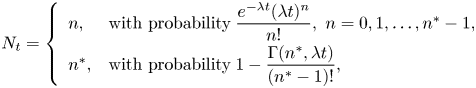 \begin{equation} N_t = \left\{\begin{array}{ll} n, & \text{with probability} \; \dfrac{e^{-\lambda t}(\lambda t)^n}{n!}, \ n=0,1,\ldots,n^*-1, \\[6pt] n^*, & \text{with probability} \; 1 - \dfrac{\Gamma(n^*,\lambda t)}{(n^*-1)!}, \end{array}\right. \end{equation}
or alternatively expressed in terms of the probability mass function as follows:
 \begin{equation} f_{\mathsf{SP}}(n; \lambda t, n^*) = \frac{e^{-\lambda t}(\lambda t)^n}{n!} {1}_{\{n \lt n^*\}} + \left(1 - \frac{\Gamma(n^*,\lambda t)}{(n^*-1)!}\right) {1}_{\{n= n^*\}}. \end{equation}
Figure 4. A stopped Poisson (SP) process which generates at most  $n^\ast$ jumps.
It is obvious that as  $t$ gets short or as $n^\ast$ gets large, the stopped Poisson process should be close to a standard Poisson process. The closeness of the two versions depends on the relation between the concerned $t$, the selected $n^\ast$, as well as the Poisson intensity $\lambda$. As we are interested in options with not very long maturities (e.g., 1, 3, and 6 months, during which jumps are not expected to happen too many times), such an assumption appears to be reasonable and should be acceptable. A proper selection of $n^\ast$ considered in this paper is $n^\ast = 5$ or $10$.
$10$.
3. Analysis of the jump accumulation under NDEJD
The integral form of a jump-diffusion model in (2.1) is given by
 \begin{equation} S_t = S_0 e^{(\mu-{\sigma^2}/{2})t + \sigma W_t + X_t}, \end{equation}
where  $X_t$ is a compound (stopped) Poisson process which describes the accumulated contributions from the series of jumps that happen in $[0,t]$:
 \begin{equation} X_t = \sum_{j=1}^{N_t} \ln Y_j. \end{equation}
To analyze the jump accumulation process  $X_t$, we let $X_t^{(n)} = (X_t\,|\,N_t=n)$ denote the compound Poisson process $X_t$ conditional on $N_t = n$. Moreover, we define $M_t$ as the number of positive jumps out of a total of $N_t$ jumps, and let $X_t^{(n,m)} = (X_t\,|\,N_t = n, M_t = m)$ denote $X_t^{(n)}$ conditional further on $M_t = m$. Under the assumption of the NDEJD model, we have
 \begin{equation} X_t^{(n,m)} = \sum_{j=1}^n \ln Y_j = \sum_{k=1}^m \varepsilon_k - \sum_{\ell=1}^{n-m} \tilde{\varepsilon}_\ell. \end{equation}
In the original DEJD model, since the series of positive and negative jump sizes ( $\varepsilon _k$ and $\tilde {\varepsilon }_\ell$) are homogeneous, it is clear that Erlang distribution (sum of i.i.d. exponential random variables) should play a central role in its analysis. Here, in our NDEJD model, because the exponential random variables in (3.3) are nonhomogeneous, in order to deal with their sums as well as the difference of these sums, we must resort to other distributions.
3.1. The HE and DHE distributions
Given a set of  $n$ exponential random variables $\varepsilon _i\sim \mathsf {Exp}(\eta _i)$, $i=1,\ldots,n$, each with a density function $f_{\varepsilon _i}(y) = \eta _i e^{-\eta _i y}$, $y\ge 0$. Suppose that $\eta _i\ne \eta _j$ for all $i, j = 1,\ldots,n, i\ne j$. The distribution followed by a sum of these nonhomogeneous exponential random variables is called a HE distribution (see, e.g. [Reference Ross12]), which is denoted as below:
 $$H_{(n)} = \sum_{i=1}^n \varepsilon_i\sim\mathsf{HE}(\boldsymbol{\eta}_{(n)}),\quad \text{where}\ \boldsymbol{\eta}_{(n)} = [\eta_1, \eta_2,\ldots, \eta_n] \in \mathbb{R}^n.$$
For the above nonnegative HE random variable  $H_{(n)}$, its probability density function (pdf), moment generating function (mgf), and moments are given analytically as follows.
Lemma 1. For a HE random variable  $H_{(n)}\sim \mathsf {HE}(\boldsymbol {\eta }_{(n)})$, its pdf is given by
 \begin{equation} f_{H_{(n)}}(y) = \sum_{i=1}^n\Omega(i;\boldsymbol{\eta}_{(n)}) \eta_i e^{-\eta_i y} {1}_{\{y\geq 0\}}, \end{equation}
where  $\Omega (i;\boldsymbol {\eta }_{(n)}) = \prod _{j=1, j\neq i}^n {\eta _j}/{(\eta _j-\eta _i)},$ and its mgf is given by
 \begin{equation} \mathrm{E}[e^{\alpha H_{(n)}}] = \prod_{i=1}^n \frac{\eta_i}{\eta_i-\alpha}. \end{equation}
The  $k$th moment of $H_{(n)}$, $k=1,2,\ldots$, can be obtained from the following formula
 \begin{equation} \mathrm{E}[H_{(n)}^k] = ({-}1)^k k! \,\boldsymbol{\pi} \mathbf{D}^{{-}k} \mathbf{1}, \end{equation}
where
 $$\boldsymbol{\pi}=\underbrace{[1,0,\ldots,0]}_{1\times n}, \quad \mathbf{D} = \underbrace{\left[\begin{array}{ccccc} -\eta_1 & \eta_1 & \cdots & 0 & 0 \\ 0 & -\eta_2 & \cdots & 0 & 0 \\ \cdots & \cdots & \ddots & \cdots & \cdots \\ 0 & 0 & \cdots & -\eta_{n-1} & \eta_{n-1} \\ 0 & 0 & \cdots & 0 & -\eta_n \end{array}\right]}_{n\times n}, \quad \mathbf{1} = \underbrace{\left[\begin{array}{c} 1 \\ \vdots \\ 1 \end{array}\right]}_{n\times 1}.$$
Proof. The pdf in (3.4) is derived in [Reference Ross12] pp. 309–311 and the mgf in (3.5) is obtained directly from those of the constituent exponential random variables. See Appendix A for the derivation of the moment formula in (3.6).
It is clear from (3.3) that for the analysis of  $X_t$, we need to work with the difference of two nonnegative random variables. For the convenience of our presentation, below we give a fundamental formula that will be used repeatedly in our subsequent derivations.
Lemma 2. Let  $X_1$ and $X_2$ be two continuous nonnegative random variables with density functions $f_1(x)$ and $f_2(x)$. The density function of $X_1-X_2$ is given by
 \begin{equation} g(y) = \left\{\begin{array}{ll} \displaystyle\int_0^\infty f_1(x+y) f_2(x)\, dx, & y \ge 0, \\[9pt] \displaystyle\int_0^\infty f_1(x) f_2(x-y)\, dx, & y \lt 0. \end{array}\right. \end{equation}
Proof. Suppose that  $X_1$ and $X_2$ are continuous real-valued random variables, the density function of $X_1-X_2$ takes the following (convolution) form:
 $$g(y) = \int_{-\infty}^\infty f_1(x) f_2(x-y)\, dx.$$
It simplifies to (3.7) by noting that the arguments of both density functions take nonnegative values as  $X_1$ and $X_2$ are nonnegative in our case.
Now, we introduce a new distribution which is followed by the difference of two HE random variables. Let  $\widetilde {H}_{(m)}\sim \mathsf {HE}(\boldsymbol {\tilde {\eta }}_{(m)})$ where $\boldsymbol {\tilde {\eta }}_{(m)} = [\tilde {\eta }_1, \tilde {\eta }_2,\ldots, \tilde {\eta }_m]$ $\in \mathbb {R}^m$ be another HE random variable. The distribution of the difference of $H_{(n)}$ and $\widetilde {H}_{(m)}$ is called a differenced hypoexponential (DHE) distribution, which is denoted as below:
 $$H_{(n)} - \widetilde{H}_{(m)} \sim\mathsf{DHE}(\boldsymbol{\eta}_{(n)}, \widetilde{\boldsymbol{\eta}}_{(m)}).$$
The following result shows that for this DHE distribution, the pdf, mgf, and moments can be derived in closed-form.
Lemma 3. The pdf of the DHE random variable  $H_{(n)} - \widetilde {H}_{(m)}$ is given by
 \begin{equation} f_{H_{(n)} - \widetilde{H}_{(m)}}(y) = \sum_{i=1}^n \sum_{j=1}^{m} \Omega (i;\boldsymbol{\eta}_{(n)})\Omega (j;\boldsymbol{\tilde{\eta}}_{(m)}) \frac{\eta_i\tilde{\eta}_j}{\eta_i + \tilde{\eta}_j} (e^{-\eta_i y}{1}_{\{y\geq 0\}} + e^{\tilde{\eta}_j y}{1}_{\{y \lt 0\}}). \end{equation}
Its mgf is given by
 \begin{equation} \mathrm{E}[e^{\alpha (H_{(n)}-\widetilde{H}_{(m)})}] = \left(\prod_{i=1}^n \frac{\eta_i}{\eta_i-\alpha}\right)\left(\prod_{j=1}^m \frac{\tilde{\eta}_j-\alpha}{\tilde{\eta}_j}\right). \end{equation}
The  $k$th moment of the DHE random variable, $k=1,2,\ldots$, can be expressed in terms of the moments of the constituent HE random variables as follows:
 \begin{equation} \mathrm{E}[(H_{(n)}-\widetilde{H}_{(m)})^k] =\sum_{j=0}^k \binom{k}{j}({-}1)^j\, \mathrm{E}[H_{(n)}^{k-j}] \,\mathrm{E}[\widetilde{H}_{(m)}^j]. \end{equation}
Proof. The pdf in (3.8) is obtained by (3.4) and (3.7) as follows. For  $y\ge 0$,
 \begin{align*} f_{H_{(n)} - \widetilde{H}_{(m)}}(y) & = \int_0^\infty f_{H_{(n)}}(x+y;\boldsymbol{\eta}_{(n)}) ~ f_{\widetilde{H}_{(m)}}(x;\boldsymbol{\tilde{\eta}}_{(m)}) \,dx \nonumber \\ & =\sum_{i=1}^n \sum_{j=1}^m \Omega (i;\boldsymbol{\eta}_{(n)})\Omega (j;\boldsymbol{\tilde{\eta}}_{(m)}) \frac{\eta_i\tilde{\eta}_j}{\eta_i + \tilde{\eta}_j} e^{-\eta_i y}, \end{align*}
whereas for  $y \lt 0$,
 \begin{align*} f_{H_{(n)} - \widetilde{H}_{(m)}}(y) & = \int_0^\infty f_{H_{(n)}}(x;\boldsymbol{\eta}_{(n)}) ~ f_{\widetilde{H}_{(m)}}(x-y;\boldsymbol{\tilde{\eta}}_{(m)}) \,dx \nonumber \\ & =\sum_{i=1}^n \sum_{j=1}^{m} \Omega (i;\boldsymbol{\eta}_{(n)})\Omega (j;\boldsymbol{\tilde{\eta}}_{(m)}) \frac{\eta_i\tilde{\eta}_j}{\eta_i + \tilde{\eta}_j} e^{\tilde{\eta}_j y}. \end{align*}
The mgf in (3.9) is obtained from the mgf of the two constituent HE random variables. The moment formula in (3.10) is obtained from the binomial theorem.
3.2. The distribution of the jump accumulation
Now that the HE and DHE distributions are well defined, the (conditional) jump accumulation process in (3.3) can be written as  $X_t^{(n,m)} = H_{(m)} - \widetilde {H}_{(n-m)}$ which follows a DHE distribution with density function given in Lemma 3. The unconditional version of $X_t^{(n,m)}$ can be written as
 \begin{equation} X_t = \sum_{j=1}^{N_t} \ln Y_j = H_{(M_t)} - \widetilde{H}_{(N_t-M_t)} = \sum_{k=1}^{M_t} \varepsilon_k - \sum_{\ell=1}^{N_t-M_t} \tilde{\varepsilon}_\ell. \end{equation}
Its distribution can be obtained by unconditioning on  $N_t=n$ and $M_t=m$ as follows.
Proposition 4. The pdf of  $X_t$ is given by
 \begin{align*} & f_{X_t}(y) = e^{-\lambda t}\delta(y) \nonumber\\ & \quad + \sum_{n=1}^{n^*} f_{\mathsf{SP}}(n;\lambda t) \left[p^n \sum_{k=1}^n\Omega(k;\boldsymbol{\eta}_{(n)}) \eta_k e^{-\eta_k y} {1}_{\{y\geq 0\}} + (1-p)^n \sum_{\ell=1}^n\Omega(\ell;\widetilde{\boldsymbol{\eta}}_{(n)}) \eta_\ell e^{\eta_\ell y} {1}_{\{y \lt 0\}}\right] \nonumber \\ & \quad + \sum_{n=2}^{n^*} \sum_{m=1}^{n-1} f_{\mathsf{SP}}(n;\lambda t) \left[\binom{n}{m}p^m(1-p)^{n-m}\vphantom{\sum_{\ell=1}^{n-m}}\right.\nonumber\\ & \quad \times\left.\sum_{k=1}^m \sum_{\ell=1}^{n-m} \Omega (k;\boldsymbol{\eta}_{(m)})\Omega (\ell;\boldsymbol{\tilde{\eta}}_{(n-m)}) \, \frac{\eta_k\tilde{\eta}_\ell}{\eta_k + \tilde{\eta}_\ell} (e^{-\eta_k y}{1}_{\{y\geq 0\}} + e^{\tilde{\eta}_\ell y}{1}_{\{y \lt 0\}})\right], \end{align*}
where  $\delta (y)$ is the Dirac delta function. The mgf of $X_t$ is given by
 \begin{align} \mathrm{E}[e^{\alpha X_t}] & = \mathrm{E}[e^{\alpha (\sum_{k=1}^{M_t} \varepsilon_k - \sum_{\ell=1}^{N_t-M_t} \tilde{\varepsilon}_\ell)}] \nonumber\\ & = e^{-\lambda t} + \sum_{n=1}^{n^*} f_{\mathsf{SP}}(n;\lambda t) \left[p^n \prod_{k=1}^n \frac{\eta_k}{\eta_k-\alpha} + (1-p)^n \prod_{\ell=1}^n \frac{\tilde{\eta}_\ell-\alpha}{\tilde{\eta}_\ell} \right] \nonumber\\ & \quad + \sum_{n=2}^{n^*} \sum_{m=1}^{n-1} f_{\mathsf{SP}}(n;\lambda t) \left[\binom{n}{m}p^m(1-p)^{n-m} \left(\prod_{k=1}^m \frac{\eta_k}{\eta_k-\alpha}\right)\left(\prod_{\ell=1}^{n-m} \frac{\tilde{\eta}_\ell-\alpha}{\tilde{\eta}_\ell}\right)\right]. \end{align}
The  $k$th moments of $X_t$, $k=1,2,\ldots$, are given by
 \begin{equation} \mathrm{E}[X_t^k] = \sum_{n=0}^{n^*}\sum_{m=0}^{n} f_{\mathsf{SP}}(n;\lambda t) \binom{n}{m}p^m(1-p)^{n-m} \left[\sum_{j=0}^k \binom{k}{j}({-}1)^j\, \mathrm{E}[H_{(m)}^{k-j}] \,\mathrm{E}[\widetilde{H}_{(n-m)}^j]\right], \end{equation}
where we define  $H_{(0)} = \widetilde {H}_{(0)} = 0$ and $H_{(0)}^0 = \widetilde {H}_{(0)}^0 = 1$.
Proof. For a given  $N_t = n\ge 1$, the probability of $M_t = m$ is $\binom {n}{m}p^m(1-p)^{n-m}$. Therefore, $X_t^{(n)}$ can be expressed as a mixture of HE and DHE random variables as described below:
 $$X_t^{(n)} = \left\{\begin{array}{ll} X^{(n,n)} = H_{(n)}, & \text{with prob}\ p^n\ \text{(when}\ m=n), \\ X^{(n,0)} ={-}\widetilde{H}_{(n)}, & \text{with prob}\ (1-p)^n\ \text{(when}\ m=0),\\ X^{(n,m)} = H_{(m)} -\widetilde{H}_{(n-m)}, & \text{with prob}\ \binom{n}{m}p^m(1-p)^{n-m},\ m=1,\ldots,n-1. \end{array}\right.$$
Moreover, its unconditional version  $X_t$ is a mixture of 0 and $X_t^{(n)}$ where $n\ge 1$:
 $$X_t = \left\{\begin{array}{ll} 0, & \text{for} \ N_t=0\ \text{with probability}\ e^{-\lambda t}, \\ X_t^{(n)}, & \text{for} \ N_t = n \ge 1\ \text{with probability}\ f_{\mathsf{SP}}(n;\lambda t). \end{array}\right.$$
The claimed results are obtained by unconditioning on  $N_t$ and $M_t$. Specifically, the pdf is
 \begin{align*} f_{X_t}(y) & = e^{-\lambda t}\delta(y) + \sum_{n=1}^{n^*} f_{\mathsf{SP}}(n;\lambda t) [p^n f_{H_{(n)}}(y;\boldsymbol{\eta}_{(n)}) + (1-p)^n f_{\widetilde{H}_{(n)}}({-}y;\widetilde{\boldsymbol{\eta}}_{(n)})]\\ & \quad +\sum_{n=2}^{n^*} \sum_{m=1}^{n-1} f_{\mathsf{SP}}(n;\lambda t) \left[\binom{n}{m}p^m(1-p)^{n-m} f_{H_{(m)} - \widetilde{H}_{(n-m)}}(y; \boldsymbol{\eta}_{(m)},\boldsymbol{\tilde{\eta}}_{(n-m)})\right], \end{align*}
which leads to (3.12). The mgf in (3.12) is obtained in a similar way. The  $k$th moment formula (3.13) is obtained from its conditional version by using the binomial theorem:
 $$\mathrm{E}[(X_t^{(n,m)})^k]= \mathrm{E}[(H_{(m)}-\widetilde{H}_{(n-m)})^k] =\sum_{j=0}^k \binom{k}{j}({-}1)^j \,\mathrm{E}[H_{(m)}^{k-j}]\, \mathrm{E}[\widetilde{H}_{(n-m)}^j].$$
The density function of  $X_t$ is in fact a mixture of a discrete random variable (i.e., a constant 0 corresponding to $N_t = 0$; it is described by the Dirac delta function in (3.12)) and many continuous (HE, DHE) random variables. A typical density function is depicted in Figure 5 where $x=0$ is a point carrying nonzero probability measure.
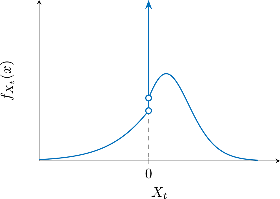
Figure 5. The density function of  $X_t$ where the delta function at $x=0$ corresponds to $N_t = 0$.
4. Option pricing under the proposed NDEJD model
In this section, we derive the risk-neutral stock return distribution, which is used to derive the European option pricing formula. We start with the stock return distribution.
4.1. The risk-neutral stock return distribution
Let  $T$ denote the maturity time of the option, and the time variable $t$ as seen in previous sections is now replaced by the constant $T$ for convenience. Let $R_T$ denote the stock return over the time period $[0,T]$. By (3.1), we have
 \begin{equation} R_T = \ln\left(\frac{S_T}{S_0}\right) = \left(\mu - \frac{\sigma^2}{2}\right) T + \sigma W_T + X_T. \end{equation}
It is clear that  $R_T$ can be seen as a normal random variable (diffusion) added to the compound Poisson random variable (jump accumulation) $X_T$. The key to the analysis is the treatment of the sum and difference between a normal and the HE/DHE distributions.
When it comes to option pricing, we need to consider the risk-neutral measure under which the martingale condition must hold, that is,  $\mathrm {E}[S_T] = S_0 e^{(r-q)T}$ (where $r$ and $q$ stand for the risk-free rate and stock dividend yield). The free variable $\mu$ in (4.1) can be adjusted to make this condition hold, that is, $\mu = r - q - \chi$ where
 \begin{align} \chi & =\frac{1}{T}\ln(\mathbb{E}[e^{X_T}]) \nonumber\\ & =\frac{1}{T}\ln\left[e^{-\lambda T} + \sum_{n=1}^{n^*} f_{\mathsf{SP}}(n;\lambda T) \left(p^n \prod_{k=1}^n \frac{\eta_k}{\eta_k-1} + (1-p)^n \prod_{\ell=1}^n \frac{\tilde{\eta}_\ell-1}{\tilde{\eta}_\ell} \right) \right. \nonumber\\ & \quad \left. +\sum_{n=2}^{n^*} \sum_{m=1}^{n-1} f_{\mathsf{SP}}(n;\lambda T) \binom{n}{m}p^m(1-p)^{n-m} \left(\prod_{k=1}^m \frac{\eta_k}{\eta_k-1}\right)\left(\prod_{\ell=1}^{n-m} \frac{\tilde{\eta}_\ell-1}{\tilde{\eta}_\ell}\right)\right]. \end{align}
Note that  $\chi$ defined above may have dependence on $T$. In (4.1), let $\nu _T = (\mu -{\sigma ^2}/{2})T = (r-q-\chi -{\sigma ^2}/{2})T$, then we have the following simpler expression for stock return under the risk-neutral measure
 \begin{equation} R_T = \nu_T + \sigma W_T + X_T. \end{equation}
For the convenience of the subsequent analysis, let us introduce the following three new distributions that are extended from HE and DHE distributions (where  $Z \sim \mathsf {N}(0,\sigma ^2)$):
• NHE $^+$ distribution, defined as the sum of normal and HE distributions, that is,
$$Z + H_{(n)} \sim\mathsf{{NHE}}^+(\sigma^2,\boldsymbol{\eta}_{(n)}).$$
$^+$ distribution, defined as the sum of normal and HE distributions, that is,
$$Z + H_{(n)} \sim\mathsf{{NHE}}^+(\sigma^2,\boldsymbol{\eta}_{(n)}).$$
• NHE
$^-$ distribution, defined as the difference of normal and HE distributions, that is,
$$Z - \widetilde{H}_{(n)} \sim\mathsf{{NHE}}^-(\sigma^2,\widetilde{\boldsymbol{\eta}}_{(n)}).$$
• NDHE distribution, defined as the sum of normal and DHE distributions, that is,
$$Z + H_{(n)} - \widetilde{H}_{(m)}\sim\mathsf{NDHE}(\sigma^2,\boldsymbol{\eta}_{(n)}, \widetilde{\boldsymbol{\eta}}_{(m)}).$$


The following lemma shows that the density functions for the above three distributions can be derived in closed-form.
Lemma 5. The density functions of the NHE $^+$, NHE $^-$, and NDHE distributions as defined above are given respectively by
 \begin{align} f_{Z+H_{(n)}}(y) & = \phi^{+}(y;\sigma^2,\boldsymbol{\eta}_{(n)}) = \sum_{i=1}^n\Omega(i;\boldsymbol{\eta}_{(n)})\eta_i e^{{(\sigma\eta_i)^2}/{2}-y\eta_i}\Phi\left(\frac{y}{\sigma}-\sigma\eta_i\right), \end{align}
 \begin{align} f_{Z-\widetilde{H}_{(n)}}(y) & =\phi^{-}(y;\sigma^2,\widetilde{\boldsymbol{\eta}}_{(n)}) = \sum_{i=1}^n\Omega(i;\widetilde{\boldsymbol{\eta}}_{(n)}) \tilde{\eta}_i e^{{(\sigma\tilde{\eta}_i)^2}/{2}+y\tilde{\eta}_i} \Phi\left(\frac{-y}{\sigma} - \sigma\tilde{\eta}_i \right), \end{align}
 \begin{align} f_{Z + H_{(n)} -\widetilde{H}_{(m)}}(y) & = \varphi(y;\sigma^2,\boldsymbol{\eta}_{(n)},\widetilde{\boldsymbol{\eta}}_{(m)}) = \sum_{i=1}^n \sum_{j=1}^m \Omega (i;\boldsymbol{\eta}_{(n)})\Omega (j;\boldsymbol{\tilde{\eta}}_{(m)})\left[\frac{\eta_i\widetilde{\eta_j}}{\eta_i + \tilde{\eta}_j}\right. \nonumber\\ & \quad \left.\times\left(e^{{(\sigma\eta_i)^2}/{2}-y\eta_i} \Phi\left(\frac{y}{\sigma}-\sigma\eta_i\right) +e^{{(\sigma\tilde{\eta}_j)^2}/{2}+y\tilde{\eta}_j}\Phi\left(\frac{-y}{\sigma}-\sigma\tilde{\eta}_j\right) \right)\right]. \end{align}
Proof. Firstly, by using (3.4) together with (3.7) (Lemma 2), we may derive
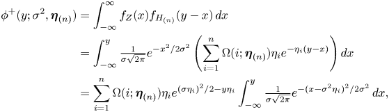 \begin{align*} \phi^{+}(y;\sigma^2,\boldsymbol{\eta}_{(n)}) & = \int_{-\infty}^\infty f_{Z}(x) f_{H_{(n)}}(y-x) \,dx \\ & =\int_{-\infty}^y \tfrac{1}{\sigma\sqrt{2\pi}} e^{-{x^2}/{2\sigma^2}} \left(\sum_{i=1}^n\Omega(i;\boldsymbol{\eta}_{(n)}) \eta_i e^{-\eta_i(y-x)}\right) dx \nonumber\\ & = \sum_{i=1}^n\Omega(i;\boldsymbol{\eta}_{(n)}) \eta_i e^{{(\sigma\eta_i)^2}/{2}-y\eta_i} \int_{-\infty}^y \tfrac{1}{\sigma\sqrt{2\pi}} e^{-{(x-\sigma^2\eta_i)^2}/{2\sigma^2}}\, dx, \end{align*}
which leads to (4.4). The formula (4.5) for  $\phi ^-(y;\sigma ^2,\boldsymbol {\eta }_{(n)})$ can be derived in a similar way. Lastly, by using (3.8), we derive
 \begin{align*} \varphi(y;\sigma^2,\boldsymbol{\eta}_{(n)},\widetilde{\boldsymbol{\eta}}_{(m)}) & = \int_{-\infty}^\infty f_{Z}(x) f_{H_{(n)} - \widetilde{H}_{(m)}}(y-x) \,dx \nonumber \\ & =\sum_{i=1}^n \sum_{j=1}^m \Omega (i;\boldsymbol{\eta}_{(n)})\Omega (j;\boldsymbol{\tilde{\eta}}_{(m)}) \nonumber \\ & \quad \times \int_{-\infty}^\infty f_{Z}(x) \left(\frac{\tilde{\eta}_j}{\eta_i + \tilde{\eta}_j} ~f_{\varepsilon_i}(x-y) + \frac{\eta_i}{\eta_i + \tilde{\eta}_j} ~f_{\tilde{\varepsilon}_j}(y-x)\right) dx, \end{align*}
which leads to (4.6).
Using the above results, the density function of  $R_T$ can be expressed in terms of the $\phi ^+$, $\phi ^-$, and $\varphi$ functions as given in (4.4), (4.5), and (4.6).
Proposition 6. The density function of  $R_T$ is given by
 \begin{align} f_{R_T}(y) & = \frac{1}{\sqrt{2\pi\sigma^2 T}}e^{-({(y-\nu_T)^2}/{2\sigma^2 T}+\lambda T)} \nonumber\\ & \quad +\sum_{n=1}^{n^*} f_{\mathsf{SP}}(n;\lambda T) [p^n \phi^+(y-\nu_T;\sigma^2 T, \boldsymbol{\eta}_{(n)}) + (1-p)^n \phi^-(y-\nu_T;\sigma^2 T, \widetilde{\boldsymbol{\eta}}_{(n)})] \nonumber\\ & \quad +\sum_{n=2}^{n^*} \sum_{m=1}^{n-1} f_{\mathsf{SP}}(n;\lambda T)\left[\binom{n}{m}p^m(1-p)^{n-m}\varphi(y-\nu_T;\sigma^2 T, \boldsymbol{\eta}_{(m)}, \widetilde{\boldsymbol{\eta}}_{(n-m)})\right], \end{align}
where  $\nu _T = (r-q-\chi -{\sigma ^2}/{2})T$ with $\chi$ defined in (4.2).
Proof. Conditional on  $N_T = n$ ( $n\ge 1$), $M_T = m$ ( $m = 0,1,\ldots,n$), we have
 $$R_T^{(n,m)} = \nu_T + \sigma W_T + X_T^{(n,m)}.$$
Since  $\sigma W_T\sim \mathsf {N}(0,\sigma ^2 T)$, it is clear that
• When
$m=n$ (where $n\ge 1$):
$$\sigma W_T+ X_T^{(n,m)} = \sigma W_T + \sum_{i=1}^n \varepsilon_i\sim\mathsf{NHE}^+(\sigma^2 T, \boldsymbol{\eta}_{(n)}).$$
• When
$m=0$ (where $n\ge 1$):
$$\sigma W_T + X_T^{(n,m)} = \sigma W_T - \sum_{i=1}^n \tilde{\varepsilon}_i\sim\mathsf{NHE}^-(\sigma^2 T, \widetilde{\boldsymbol{\eta}}_{(n)}).$$
• When
$1\le m\le n-1$ (where $n\ge 2$):
$$\sigma W_T + X_T^{(n,m)} = \sigma W_T + \sum_{i=1}^m \varepsilon_i - \sum_{j=1}^{n-m} \tilde{\varepsilon}_j\sim\mathsf{NDHE}(\sigma^2 T, \boldsymbol{\eta}_{(m)}, \widetilde{\boldsymbol{\eta}}_{(n-m)}).$$


The density function of  $R_T$ is then obtained by unconditioning on $N_t$ and $M_t$.
The mgf of  $R_T$ can be easily obtained as a product of a normal mgf and (3.12). As to the $k$th moment of $R_T$, its general form can be obtained as
 \begin{equation} \mathrm{E}[R_T^k] = \sum_{j=0}^{k} \binom{k}{j}\, \mathrm{E}[(\nu_T+\sigma W_T)^j]\, \mathrm{E}[X_T^{k-j}]. \end{equation}
We are mainly interested in the first four moments of  $R_T$, which can be obtained together with the moments of normal random variable $\nu _T + \sigma W_T\sim \mathsf {N}(\nu _T,\sigma ^2 T)$ as given below:
 \begin{align*} & \mathrm{E}[\nu_T+\sigma W_T] = \nu_T, \quad \mathrm{E}[(\nu_T+\sigma W_T)^2] = \nu_T^2 + \sigma^2 T, \\ & \mathrm{E}[(\nu_T+\sigma W_T)^3] = \nu_T^3 + 3\nu_T\sigma^2 T, \quad \mathrm{E}[(\nu_T+\sigma W_T)^4] = \nu_T^4 + 6\nu_T^2\sigma^2 T + 3\sigma^4 T^2. \end{align*}
4.2. Option pricing formula
We are now in a position to derive the pricing formula for a European option. Consider a call option with strike price  $K$ and maturity time $T$. Its price is given by the following risk-neutral pricing formula:
 \begin{equation} C = e^{{-}rT}\,\mathrm{E}[(S_T-K)^+] = e^{{-}rT}\,\mathrm{E}[S_T {1}_{\{S_T\ge K\}}] - Ke^{{-}rT}\mathrm{P}(S_T\ge K). \end{equation}
To deal with the probability  $\mathrm {P}(S_T\ge K)$ in the second term, we define the complementary distribution functions of the NHE $^+$, NHE $^-$, and NDHE distributions (where $Z \sim \mathsf {N}(0,\sigma ^2)$).
 \begin{align*} \bullet \quad & \mathrm{U}^+(x;\sigma^2,\boldsymbol{\eta}_{(n)}) = \mathrm{P}(Z + H_{(n)} \geq x),\\ \bullet \quad & \mathrm{U}^-(x;\sigma^2,\widetilde{\boldsymbol{\eta}}_{(m)}) =\mathrm{P}(Z - \widetilde{H}_{(m)} \geq x),\\ \bullet \quad & \mathrm{V}(x;\sigma^2,\boldsymbol{\eta}_{(n)},\widetilde{\boldsymbol{\eta}}_{(m)}) =\mathrm{P}(Z + H_{(n)} - \widetilde{H}_{(m)} \geq x). \end{align*}
As it turns out, the closed-form expressions of these functions can be derived.
Lemma 7. The closed-form expressions of the three functions  $\mathrm {U}^+, \mathrm {U}^-, \mathrm {V}$ as defined above are respectively given by
 \begin{align} \mathrm{U}^+(x;\sigma^2,\boldsymbol{\eta}_{(n)}) & = \sum_{i=1}^n\Omega(i;\boldsymbol{\eta}_{(n)})\left(\Phi\left(-\frac{x}{\sigma}\right) + e^{{(\sigma\eta_i)^2}/{2}-x\eta_i} \Phi\left(\frac{x}{\sigma} - \sigma\eta_i \right)\right), \end{align}
 \begin{align} \mathrm{U}^-(x;\sigma^2,\widetilde{\boldsymbol{\eta}}_{(m)}) & = \sum_{j=1}^n\Omega(j;\boldsymbol{\eta}_{(m)})\left(\Phi\left(-\frac{x}{\sigma}\right) - e^{{(\sigma\eta_j)^2}/{2}+x\eta_j} \Phi\left(\frac{-x}{\sigma} - \sigma\eta_j \right)\right), \end{align}
 \begin{align} \mathrm{V}(x;\sigma^2,\boldsymbol{\eta}_{(n)},\widetilde{\boldsymbol{\eta}}_{(m)}) & = \sum_{i=1}^n \sum_{j=1}^m \Omega (i;\boldsymbol{\eta}_{(n)})\Omega (j;\boldsymbol{\tilde{\eta}}_{(m)}) \nonumber\\ & \quad \times \left[\frac{\tilde{\eta}_j}{\eta_i + \tilde{\eta}_i}\left(\Phi\left(-\frac{x}{\sigma}\right) + e^{\frac{(\sigma\eta_i)^2}{2}-x\eta_i}\Phi\left(\frac{x}{\sigma} - \sigma\eta_i \right)\right)\right.\nonumber\\ & \quad \left. + \frac{\eta_i}{\eta_i + \tilde{\eta}_j}\left(\Phi\left(-\frac{x}{\sigma}\right) - e^{\frac{(\sigma\tilde{\eta}_j)^2}{2}+x\tilde{\eta}_j} \Phi\left(\frac{-x}{\sigma} - \sigma\tilde{\eta}_j \right)\right)\right]. \end{align}
Proof. See Appendix B.
Next, to deal with the expected value  $\mathrm {E}[S_T {1}_{\{S_T\ge K\}}]$ in (4.9), we need to further define the following three functions related to the NHE $^+$, NHE $^-$, and NDHE distributions.
 \begin{align*} \bullet \quad & \mathrm{\Pi}^+(x;\sigma^2,\boldsymbol{\eta}_{(n)})= \mathrm{E}[e^{Z + H_{(n)}}{1}_{\{Z + H_{(n)} \geq x\}}],\\ \bullet \quad & \mathrm{\Pi}^-(x;\sigma^2,\widetilde{\boldsymbol{\eta}}_{(m)})= \mathrm{E}[e^{Z - \widetilde{H}_{(m)}}{1}_{\{Z - \widetilde{H}_{(m)} \geq x\}}],\\ \bullet \quad & \mathrm{\Lambda}(x;\sigma^2,\boldsymbol{\eta}_{(n)},\widetilde{\boldsymbol{\eta}}_{(m)}) =\mathrm{E}[e^{Z + H_{(n)} - \widetilde{H}_{(m)}}{1}_{\{Z + H_{(n)} - \widetilde{H}_{(m)} \geq x\}}]. \end{align*}
Fortunately, once again we are able to derive their closed-form results, as seen subsequently.
Lemma 8. Suppose that  $\eta _i \gt 1$, $i=1,\ldots,n$. The closed-form expressions of the three functions $\mathrm {\Pi }^+, \mathrm {\Pi }^-, \mathrm {\Lambda }$ as defined above are respectively given by
 \begin{align} \mathrm{\Pi}^+(x;\sigma^2,\boldsymbol{\eta}_{(n)}) & = \sum_{i=1}^n\Omega(i;\boldsymbol{\eta}_{(n)})\frac{\eta_i e^{\frac{(\sigma\eta_i)^2}{2}}}{\eta_i-1} \nonumber\\ & \quad \times \left(e^{-{(\eta_i^2-1)\sigma^2}/{2}}\Phi\left(\frac{-x}{\sigma}+\sigma\right) + e^{-(\eta_i-1)x}\Phi\left(\frac{x}{\sigma}-\sigma\eta_i\right)\right), \end{align}
 \begin{align} \mathrm{\Pi}^-(x;\sigma^2,\widetilde{\boldsymbol{\eta}}_{(m)}) & = \sum_{j=1}^m\Omega(j;\widetilde{\boldsymbol{\eta}}_{(m)})\,\frac{\tilde{\eta}_j e^{\frac{(\sigma\tilde{\eta}_j)^2}{2}}}{\tilde{\eta}_j+1} \nonumber\\ & \quad \times \left(e^{-{(\tilde{\eta}_j^2-1)\sigma^2}/{2}}\Phi\left(\frac{-x}{\sigma}+\sigma\right) - e^{(\tilde{\eta}_j+1)x}\Phi\left(\frac{-x}{\sigma}-\sigma\tilde{\eta}_j\right)\right), \end{align}
 \begin{align} \mathrm{\Lambda}(x;\sigma^2,\boldsymbol{\eta}_{(n)}, \widetilde{\boldsymbol{\eta}}_{(m)}) & = \sum_{i=1}^n \sum_{j=1}^m \Omega (i;\boldsymbol{\eta}_{(n)})\Omega (j;\boldsymbol{\tilde{\eta}}_{(m)})\frac{\eta_i\widetilde{\eta_j}}{\eta_i + \tilde{\eta}_j} \nonumber\\ & \quad \times{\times}\left[\frac{ e^{{(\sigma\eta_i)^2}/{2}}}{\eta_i-1}\left(e^{-{(\eta_i^2-1)\sigma^2}/{2}}\Phi \left(\frac{-x}{\sigma}+\sigma\right) + e^{-(\eta_i-1)x}\Phi\left(\frac{x}{\sigma}-\sigma\eta_i\right)\right) \right. \nonumber\\ & \quad + \left. \frac{e^{{(\sigma\tilde{\eta}_j)^2}/{2}}}{\tilde{\eta}_j+1} \left(e^{-{(\tilde{\eta}_j^2-1)\sigma^2}/{2}}\Phi\left(\frac{-x}{\sigma}+\sigma\right) - e^{(\tilde{\eta}_j+1)x}\Phi\left(\frac{-x}{\sigma}-\sigma\tilde{\eta}_j\right)\right)\right]. \end{align}
Proof. See Appendix C.
Remark. It is worth noting that in Lemma 8, we require  $\eta _i \gt 1$, $i=1,\ldots,n$ to prevent the integrations in (4.13) and (4.15) from blowing up. There is no such requirement for $\tilde {\eta }_j$, $j=1,\ldots,m$ in (4.14) and (4.15) because the integrations related to $\tilde {\eta }_j$ are finite for all positive $\tilde {\eta }_j$. See Appendix C for details.
Armed with Lemmas 7 and 8, we are now ready to derive the European call option price under the proposed NDEJD model.
Proposition 9. The price of a European call option with strike price  $K$ and maturity time $T$ under the NDEJD model is given by
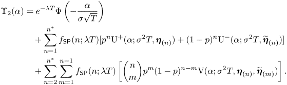
 \begin{equation} C = S_0 e^{-(q + {\sigma^2}/{2} + \chi)T} \,\mathrm{\Upsilon}_1(\alpha) - K e^{{-}rT} \mathrm{\Upsilon}_2(\alpha), \end{equation}
where  $\alpha = \ln (K/S_0)-\nu _T$ and $\mathrm {\Upsilon }_1(\alpha )$, $\mathrm {\Upsilon }_2(\alpha )$ are respectively given by
 \begin{align} \mathrm{\Upsilon}_1(\alpha) & = e^{{\sigma^2T}/{2}-\lambda T}\Phi\left(\frac{\sigma^2T - \alpha}{\sigma\sqrt{T}}\right) \nonumber\\ & \quad + \sum_{n=1}^{n^*} f_{\mathsf{SP}}(n;\lambda T) [p^n \Pi^+(\alpha;\sigma^2 T,\boldsymbol{\eta}_{(n)}) + (1-p)^n \Pi^-(\alpha;\sigma^2 T,\widetilde{\boldsymbol{\eta}}_{(n)})] \nonumber\\ & \quad + \sum_{n=2}^{n^*} \sum_{m=1}^{n-1} f_{\mathsf{SP}}(n;\lambda T) \left[\binom{n}{m}p^m(1-p)^{n-m} \Lambda(\alpha;\sigma^2 T,\boldsymbol{\eta}_{(n)}, \widetilde{\boldsymbol{\eta}}_{(m)})\right], \end{align}
 \begin{align} \mathrm{\Upsilon}_2(\alpha) & = e^{-\lambda T}\Phi\left(-\frac{\alpha}{\sigma\sqrt{T}}\right)\nonumber\\ & \quad + \sum_{n=1}^{n^*} f_{\mathsf{SP}}(n;\lambda T)[p^n \mathrm{U}^+(\alpha;\sigma^2 T,\boldsymbol{\eta}_{(n)}) + (1-p)^n \mathrm{U}^-(\alpha;\sigma^2 T,\widetilde{\boldsymbol{\eta}}_{(n)})] \nonumber\\ & \quad + \sum_{n=2}^{n^*} \sum_{m=1}^{n-1} f_{\mathsf{SP}}(n;\lambda T) \left[\binom{n}{m}p^m(1-p)^{n-m} \mathrm{V}(\alpha;\sigma^2 T,\boldsymbol{\eta}_{(n)},\widetilde{\boldsymbol{\eta}}_{(m)})\right]. \end{align}
Proof. It is clear from (4.9) together with (4.3) that
 $$C = S_0 e^{-(q + {\sigma^2}/{2} + \chi)T}\,\mathrm{E}[e^{\sigma W_T + X_T}{1}_{\{\sigma W_T + X_T\ge\alpha\}}] - Ke^{{-}rT}\mathrm{P}(\sigma W_T + X_T\ge \alpha),$$
where we note that the event  $\{S_T\ge K\}$ is equivalent to the event $\{\sigma W_T + X_T\ge \alpha \}$. Let us define the two functions:
 $$\mathrm{\Upsilon}_1(\alpha) = \mathrm{E}[e^{\sigma W_T+X_T}{1}_{\{\sigma W_T+X_T\geq \alpha\}}],\quad \mathrm{\Upsilon}_2(\alpha) = \Pr(\sigma W_T+X_T\geq \alpha).$$
Following the unconditioning technique on  $N_t$ and $M_t$ as in the proof of Proposition 6, the two functions can be derived as claimed using the results in Lemmas 7 and 8.
5. Numerical results
Our numerical results are provided to look into the effects of nonhomogeneous jump sizes on stock return distributions (under the risk-neutral measure), option prices, and implied volatility smiles under the NDEJD model. In our model set-up, the series of  $\eta _k$ and $\tilde {\eta }_k$, $k=1,2,\ldots$ can take different values, but for demonstrative purpose, we assume that there is an internal structure among the series of $\eta _k$ and $\tilde {\eta }_k$ as described below:
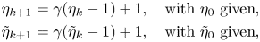 \begin{align*} \eta_{k+1} & = \gamma(\eta_k - 1) + 1,\quad \text{with}\ \eta_0\ \text{given,}\\ \tilde{\eta}_{k+1} & = \gamma(\tilde{\eta}_k - 1) + 1,\quad \text{with}\ \tilde{\eta}_0\ \text{given,} \end{align*}
where a new parameter  $\gamma$ is introduced to indicate that the series of $\eta _k$ and $\tilde {\eta }_k$ are increasing ( $\gamma \gt 1$) or decreasing ( $\gamma \lt 1$). The above formulas assume that $(\eta _k-1)$ and $(\tilde {\eta }_k-1)$ are both geometric series. The reason behind this assumption is that it ensures $\eta _k, \tilde {\eta }_k \gt 1$ for all $k$ in order to avoid the blow-up problem in (4.13)–(4.15) (such that the integrations in the functions $\mathrm {\Pi }^+$, $\mathrm {\Pi }^-$, and $\mathrm {\Lambda }$ exist). Note that $\gamma \lt 1$ ( $\gamma \gt 1$) implies that the tail distributions of the successive jump sizes are getting fatter (lighter), meaning that there is a growing (diminishing) effects from jumps.
Our benchmark model is the special case  $\gamma = 1$ which is very close to the DEJD model except that the jumps in the NDEJD with $\gamma = 1$ is driven by a stopped Poisson process (a maximal $n^\ast$ is specified) whereas the jumps in the DEJD model are driven by a standard Poisson process. Precisely speaking, they are different, but they are in fact close enough if the maturity time $T$ is short or the maximal number of jumps $n^\ast$ is large. In these cases, our benchmark NDEJD model with $\gamma = 1$ can be seen as almost identical to the original DEJD model.
5.1. Return distributions
We first present the numerical results for the risk-neutral return distributions under the NDEJD model. The basic parameters that are not related to jumps (about drift and diffusion) are  $r = 0.05$, $q = 0.01$, and $\sigma = 0.2$. Some parameters about jumps are fixed: $\lambda = 5$, $n^\ast = 10$, $\eta _{0} = 10$, and $\tilde {\eta }_{0} = 5$ ( $\tilde {\eta }_{0} \lt \eta _0$ indicates that the left tail is fatter than the right tail, as commonly seen empirically). In order to investigate the influences from the growing and diminishing effects of jumps, we consider the following parameters about jump size distributions: $p\in \{0.2, 0.5,0.8\}$, $\gamma = \{0.8, 0.9, 1.0, 1.1, 1.2\}$. Three maturity times are considered: $T\in \{0.25, 0.5, 1.0\}$.
Figure 6 shows the risk-neutral distribution of  $R_T$. The effect of maturity time $T$ can be seen from top to bottom. As $T$ grows, the distribution becomes more widely spread as expected. The effect of $p$ (the probability of seeing positive jumps) can be seen from left to right. Larger $p$ indicates that positive jumps are more likely to happen than negative jumps, and this makes the right tail fatter. The differences between left and right tails become more prominent when $T$ gets longer. In each plot, five curves are provided to show the effect of $\gamma$. We observe that when jumps have growing effects ( $\gamma \lt 1$), the distribution tends to be fatter-tailed and the left tail is generally (see the plots with $p=0.5$) lifted up more because the influences from negative jumps are stronger than those from positive jumps (this is because of our chosen parameters for the initial jump, i.e., $\tilde {\eta }_0 \lt \eta _0$). On the contrary, if the effects from jumps are diminishing ( $\gamma \gt 1$), the distribution becomes more narrowly spread with thinner tails on both sides. When $p = 0.2$, the left tail becomes much fatter because negative jumps happen more frequently than positive jumps. As $p$ gets larger, the right tails are lifted up more. This shows that positive jumps bring about more impacts to the distribution.
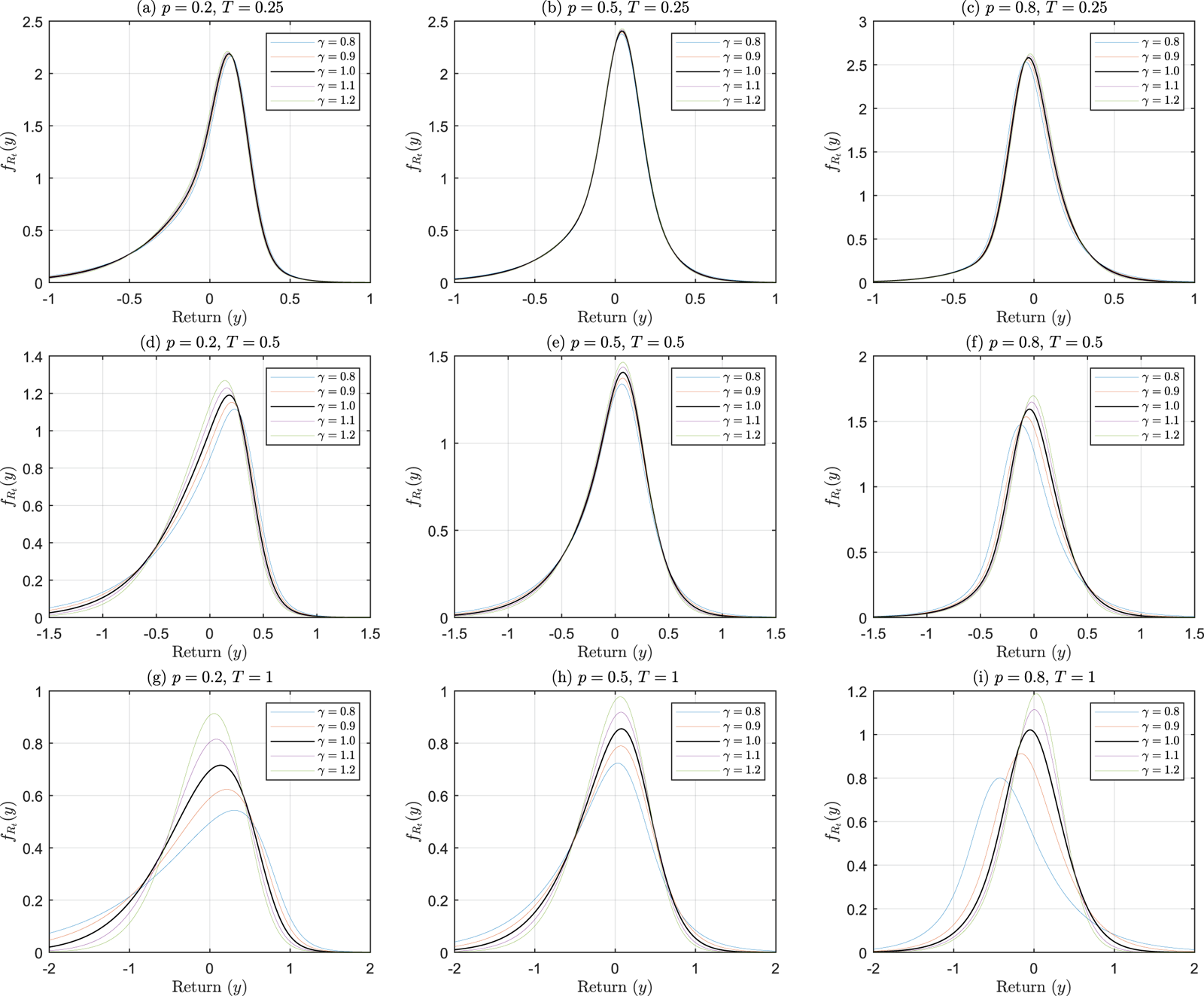
Figure 6. Return distributions (pdf) under various combinations of  $p$ and $T$.
$T$.
The basic statistics (mean, standard deviation, skewness, kurtosis) of  $R_T$ are provided in Table 1. The results for Kou's (2002) DEJD model (where jumps are driven by a Poisson process) are given below the results for the benchmark NDEJD model with $\gamma = 1$ (where jumps are driven by a stopped Poisson process with $n^\ast = 10$) in order to show that the two models are almost identical. We observe close agreements bewteen Figure 6 and Table 1, but the figures in Table 1 provide more insights. We see that as $\gamma$ gets smaller, kurtosis becomes larger but skewness becomes more negative when $p=0.2$ (left tails receive more impacts) and less negative when $p = 0.8$ (right tails receive more impacts). Moreover, it is worth pointing out that, as $T$ gets longer, the standard deviation (SD) increases as expected, but both the skewness (in absolute value) and kurtosis seem to become smaller, indicating that the distribution becomes less skewed and less fat-tailed. In contrast, however, as seen in Figure 6, the influences on both tails appear to be more prominent as $T$ gets longer. This shows that the statistical figures in Table 1 provide a different view which is not directly observable from Figure 6.
Table 1. The basic statistics of  $R_T$ under various combinations of $p$ and $T$.
$T$.
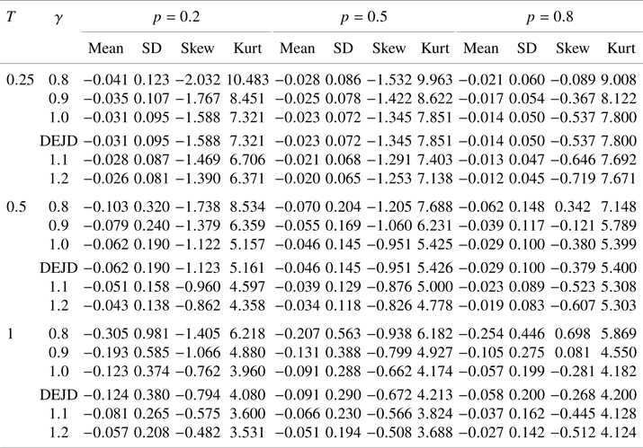
5.2. Option prices
Next, we present the numerical results about European call option prices. To investigate the nonlinear influences from  $\gamma$ and other factors on call option prices, we conduct a regression analysis. Let $M = K/S_0$ denote the moneyness for a call option (it is at-the-money if $M=1$). We consider option contracts with different moneyness $M = 0.5, 0.6,\ldots, 1.5$ and maturity $T = 0.25, 0.5, 0.75, 1.0$. Take $\gamma = 1$ (seen as almost equivalent to the DEJD model) as the benchmark and define “Bias” for the $\gamma \ne 1$ cases as the percentage error of the call option price relative to the benchmark case, that is,
 $$\text{Bias} = \frac{C_\gamma-C_{\gamma=1}}{C_{\gamma=1}}.$$
We expect that Bias is a nonlinear function of  $\gamma -1$, $p, M, T$, written as $\text {Bias} = f(\gamma -1, p, M, T)$. In our analysis, we intend to use the following quadratic formulation for the function $f$, that is,
 \begin{equation} \text{Bias} = \beta_0(p,M,T) + \beta_1(p,M,T) (\gamma-1) + \beta_2(p,M,T) (\gamma-1)^2, \end{equation}
to model the dependence of Bias on the main factor  $(\gamma -1)$. The contributions from $p, M, T$ are left to the coefficients $\beta _i(p,M,T), i=0,1,2$. Specifically, the linear, quadratic, and interactive influences that come purely from $p, M, T$ are captured by $\beta _0(p,M,T)$, whereas their interactions with $(\gamma -1)$ and $(\gamma -1)^2$ are respectively captured by $\beta _1(p,M,T)$ and $\beta _2(p,M,T)$.
Table 2 presents the estimation results of eight nested regression models based on (5.1). Model 1 is a purely linear model which takes the following form ( $c_i$ represents the coefficients)
 $$\text{Bias} = c_0 + c_1 p + c_2 M + c_3 T + c_4 (\gamma-1),\quad R^2 = 32\%.$$
Such a linear model provides a baseline level of adjusted  $R^2 = 32\%$. Model 2 adds the cross terms between $p,M,T$ and $(\gamma -1)$ to model their interactions (these cross terms are part of $\beta _1(p,M,T)$ in (5.1)), that is,
 $$\text{Bias} = c_0 + c_1 p + c_2 M + c_3 T + (c_4 + c_5 p + c_6 M + c_7 T)(\gamma-1), ~R^2 = 59\%,$$
lifting the adjusted  $R^2$ to 59%. By adding quadratic and interaction terms between $p,M,T$ to $\beta _1(p,M,T)$, the adjusted $R^2$ is improved to 62% in Model 3 and further to 70% in Model 4. The stepwise inclusions of all higher-order interaction terms increase the adjusted $R^2$ to nearly 90% in Model 8. This is our full model where $\beta _i(p,M,T)$, $i=0,1,2$ exhibit the following structure:
 \begin{align*} \beta_0 & = (c_0 + c_1 p + c_2 M + c_3 T), \\ \beta_1 & = (c_4 + c_5 p + c_6 M + c_7 T + c_8 p^2 + c_9 M^2 + c_{10} T^2 + c_{11} pM + c_{12} pT + c_{13} MT), \\ \beta_2 & = (c_{14} + c_{15} p + c_{16} M + c_{17} T + c_{18} p^2 + c_{19} M^2 + c_{20} T^2 + c_{21} pM + c_{22} pT + c_{23} MT). \end{align*}
In Table 2, the significant coefficients (marked with  $\ast$) of the nonlinear terms show that the Bias depends nonlinearly on its influencing factors (i.e., $\gamma$ as well as $p,M,T$). The significance of the coefficients in $\beta _1$ (i.e., $c_4,\ldots,c_{13}$, which are almost identical from Model 4 to Model 8) reveals that the main factor $\gamma$ may cause strong Bias (percentage error) in call price if the nonhomogeneity in jumps is not considered. The significance of the coefficients in $\beta _2$ (i.e., $c_{14},\ldots,c_{23}$) further shows that the main factor $\gamma$ influences Bias in an asymmetric way. For example, from the positiveness of $c_{14} = 3.693$ (Model 5), we see that a decrease in $\gamma$ (e.g., $1\to 0.9$) would cause a greater bias than an increase in $\gamma$ (e.g., $1\to 1.1$). The fact that many of $c_{14},\ldots,c_{23}$ (Model 8) are significant indicates that $\beta _2$ depends in a complicated nonlinear way on $p, M, T$.
Table 2. Estimation results of the nested regression models for “Bias”.
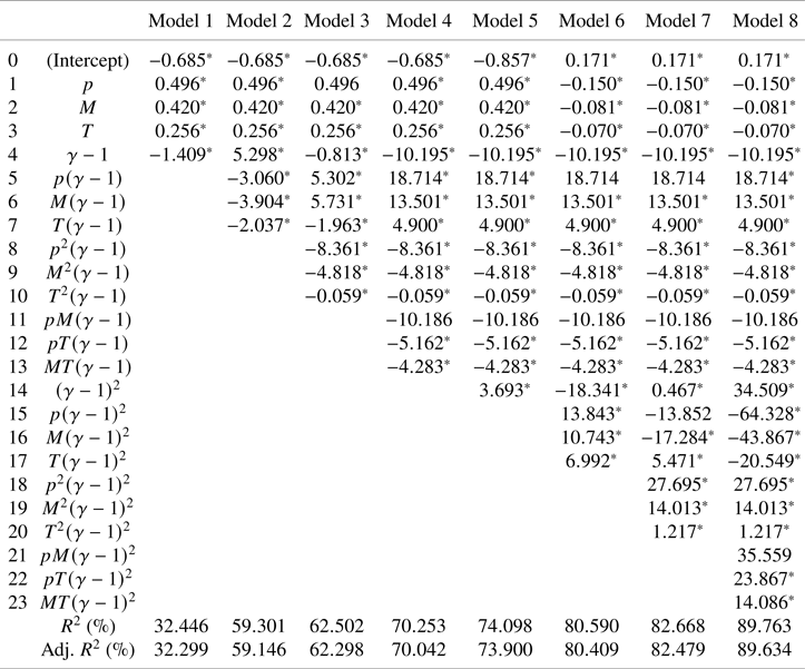
 $^\ast$Indicates that the coefficient is significant with $p$-value <0.05.
5.3. Implied volatility smiles
We move on to present our numerical results on implied volatiliy smiles which reveal the risk structure behind the model. Suppose that the market follows the proposed NDEJD model, the implied volatility  $\hat {\sigma }$ is the particular volatility in the Black–Scholes formula that gives the same option price, that is,
 $$C_{\text{NDEJD}} = C_{\text{BS}}(S_0, K, T, r, q, \hat{\sigma}),$$
where  $C_{\text {NDEJD}}$ is obtained from our pricing formula (4.16). The volatility smile ( $\hat {\sigma }$ as a function of moneyness, which is redefined as $M = \ln (K/S_0)$) is then obtained by solving the above nonlinear equation for all $M$. (See [Reference Cont and Fonseca4] for its implication and [Reference Dumas, Fleming and Whaley6] for an example of its empirical analysis.)
The results are presented in Figure 7 where the at-the-money ( $M=0$) implied volatility is fixed at 0.4 (by setting $\lambda = 2$ with $\sigma$ left free; other parameters remain the same as in Figure 6). We see that the smile curves are pulled higher (lower) when $\gamma$ decreases (increases), indicating that the level of risk is heightened (lowered) when there are growing (diminishing) impacts from jumps. The smiles for $p=0.5$ tend to be more symmetric than $p = 0.2$ or 0.8. When $p = 0.2$ (0.8), more influences are made on the left (right) tails of the return distributions, and thus the left (right) wings of the smiles are lifted or lowered more. Moreover, the smiles exhibit the highest curvature when $T = 0.25$ (which is consistent with Table 1 where higher kurtosis is seen in smaller $T$ cases). As $T$ increases, the smiles become less curved, but the differences across all $\gamma$ become more noticeable.
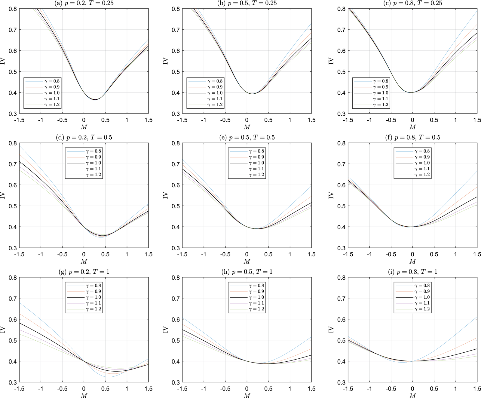
Figure 7. Implied volatility smiles under various combinations of  $p$ and $T$.
$T$.
In contrast with the above qualitative observations, below we give a quantitative analysis on how the shapes of the IV smiles vary with  $\gamma$ and other parameters. To this end, we consider a typical IV smiles as depicted in Figure 8, where ${\rm IV}_1$, ${\rm IV}_2$, and ${\rm IV}_3$ are the IV for three moneyness $M_1, M_2, M_3$ ( $M_2$ refers to the lowest point and $M_1 = M_2-1$, $M_3 = M_2+1$). The following five parameters are used to capture the main features of a typical smile curve:
•
$a = M_2$: the moneyness where the smile drops to the lowest point,•
$b = {\rm IV}_2$: the minimal level of IV at $M_2$,•
$c = {\rm IV}_3 - 2{\rm IV}_2 + {\rm IV}_1$: the curvature of the smile,•
$d = {\rm IV}_2 - {\rm IV}_1$: the (negative) slope of the left wing,•
$e = {\rm IV}_3-{\rm IV}_2$: the (positive) slope of the right wing.


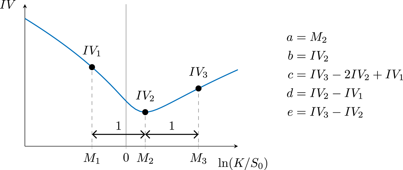
Figure 8. The features of a typical smile curve.
The five shape parameters of all IV smiles in Figure 7 are summarized in Table 3, from which we may take a closer inspection of the smile curves. It is seen from the results of parameter  $a$ that the lowest point of smiles moves leftward as $p$ gets large but it moves rightward as $T$ gets large. From the results of parameter $b$, we observe that smaller $\gamma$ leads to higher $b$ (the overall volatility level is also pulled up, as seen in every plot). The shape parameters $c$,
$c$,  $d$,
$d$,  $e$ carry more important information about the risk-neutral distributions. We observe that as either $\gamma$ or $T$ increases, the curvature $c$ decreases, indicating that the distribution becomes less fat-tailed (this is in close agreement with Table 1). The parameters $d$ and $e$ are concerned with the slopes of the left and right wings. It is observed that smaller $\gamma$ makes the two wings steeper, and therefore, the values of $|d|$ and $e$ become greater. But the parameter $p$ tends to influence one side of the smile. Smaller $p$ makes the left wing steeper, whereas greater $p$ makes the right wing steeper. All these observations are consistent with Figure 6 and Table 1.
Table 3. The five shape parameters  $a, b, c, d, e$ of IV smiles.
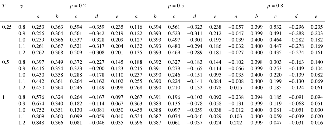
5.4. Empirical analysis
To further justify the proposed NDEJD model which exhibits a richer shape of the IV smile relative to the DEJD model as shown in the preceding subsection, we provide an empirical analysis. The standard S&P 500 index option (SPX) data are collected and the two competing models are calibrated to their implied volatility smiles for various times to maturity. The data for the whole year of 2021 are collected and analyzed; among them, eight data sets (see Table 4) are picked for our presentation. The chosen two observation dates are the very first trading days in the first half year (sets (a)(b)(c)(d)) and in the second half year (sets (e)(f)(g)(h)). For each observation day, four maturity days are considered in order to cover different times to maturity ( $\tau$). Table 4 also shows the initial index ( $S_0$), the maximal and minimal strike prices ( $K_{\rm min}$, $K_{\rm max}$), and the number of strike prices ( $n$) for each maturity date.
Table 4. Eight data sets for the comparison of model calibration.
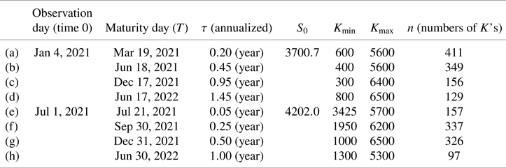
With the interest rate and dividend yield chosen as  $r = 0.01, q = 0$, we calibrate the two models to determine the model parameter set $\boldsymbol {x}$ by minimizing the sum of squared errors (SSE) of the implied volatility curve, that is,
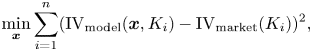 $$\min_{\boldsymbol{x}} \sum_{i=1}^n (\text{IV}_{\mathrm{model}}(\boldsymbol{x}, K_i) - \text{IV}_{\mathrm{market}}(K_i) )^2,$$
where the parameter set is  $\boldsymbol {x} = (\sigma,\lambda,\eta _0,\tilde {\eta }_0,p)$ for DEJD, and is $\boldsymbol {x} = (\sigma,\lambda,\eta _0,\tilde {\eta }_0,p,\gamma )$ for NDEJD. The results are given in Table 5, where we observe that the NDEJD parameter $\gamma$ may deviate from 1 (it could be greater or less than 1). The inclusion of $\gamma$ provides one more degree of freedom which reduces the SSE significantly, indicating the advantage of NDEJD over DEJD for these particular data sets.
Table 5. Results of model calibration.
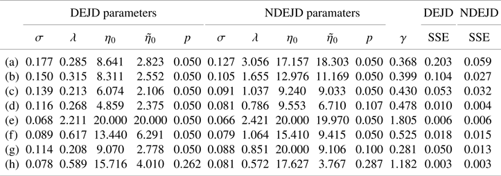
Figure 9 provides a graphical illustration of the calibration results from the eight data sets. In each plot, the horizontal axis is moneyness  $M$ which is defined to be $M = \ln (K/S_0)$. While DEJD provides satisfactory results, it is not difficult to see that our NDEJD model provides an even closer fit to the market IV smiles. In particular, the deviations between the two models are more prominent at the left ends (with large negative $M$), showing that the flexibility in NDEJD provides advantages for the options that are far-away-from-the-money. This gives a justification for the proposed NDEJD model.
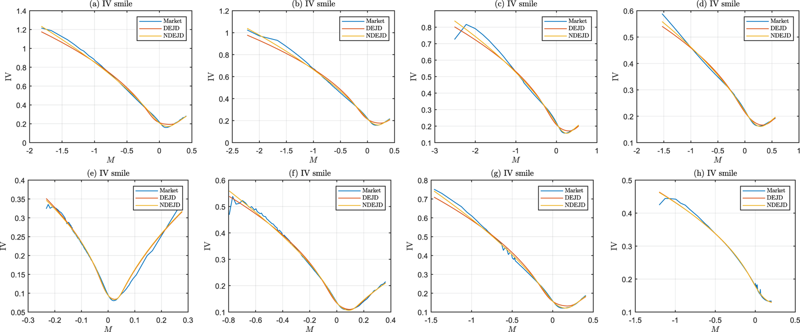
Figure 9. Graphical illustration of the calibration results in Table 5.
6. Conclusion
In this paper, we propose an extended version of the DEJD model where jump sizes follow DE distributions but are no longer i.i.d. The proposed NDEJD model can be used to capture the varying impacts from a series of jumps. For the extended model, we provide a mathematical analysis on the risk-neutral return distribution, which requires some distributions in close relation with HE distributions. Based on these distributions, we derive the European option pricing formula in closed-form. While our model allows for all the exponential parameters to take different values, our numerical analysis focuses on two scenarios where the effects from jumps are either growing or diminishing. Numerical results show that in the former scenario, the return distributions become more fatter-tailed, the option prices become significantly higher, and the implied volatility smiles are significantly heightened with higher curvature and greater slopes (in absolute value) on both wings. In contrast, in the latter scenario, the effects are not as significant. In sum, our study contributes to the option pricing literature by adding more flexibility to the popular EDJD model to adapt it for better reflecting the changing nature of jump processes.
Acknowledgments
The authors acknowledge the support from the Ministry of Science and Technology (MOST) of Taiwan under the grant number MOST-106-2410-H-011-001.
Appendix A. Proof of Lemma 1
A HE distribution is a special case of the phase-type distribution (PTD) (see, e.g., the discussion in Chapter 2 of [Reference Buchholz, Kriege and Felko2]) which is followed by the time to absorption of a finite state continuous-time Markov chain (CTMC). Consider such a chain that has  $n+1$ states, where the first $n$ states are transient and the last one is absorbing. Suppose that this CTMC moves sequentially from state $1, 2,\ldots$ until it is absorbed in state $n+1$ (see the following diagram, where the transition from state $i$ to $i+1$ has a rate of $\eta _i$, $i=1,\ldots,n$), then the total time from start to absorption follows a HE distribution. By the equation (2.12) of [Reference Buchholz, Kriege and Felko2], the density function of a HE random variable $H_{(n)}$ can be expressed in the following matrix form:
 $$f_{H_{(n)}}(x) = \boldsymbol{\pi} e^{\mathbf{D} x}\mathbf{d} \quad \text{for} \ x \geq 0,$$
where
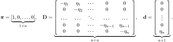 $$\boldsymbol{\pi}=\underbrace{[1,0,\ldots,0]}_{1\times n}, \quad \mathbf{D} = \underbrace{\left[\begin{array}{ccccc} -\eta_1 & \eta_1 & \cdots & 0 & 0 \\ 0 & -\eta_2 & \cdots & 0 & 0 \\ \cdots & \cdots & \ddots & \cdots & \cdots \\ 0 & 0 & \cdots & -\eta_{n-1} & \eta_{n-1} \\ 0 & 0 & \cdots & 0 & -\eta_n \end{array}\right]}_{n\times n}, \quad \mathbf{d} = \underbrace{\left[\begin{array}{c} 0 \\ 0 \\ \vdots \\ 0 \\ \eta_n \end{array}\right]}_{n\times 1}.$$
The  $k$th moment of $H_{(n)}$ as seen in (3.6) can be derived as follows:
 $$\mathrm{E}[H_{(n)}^k] = \int_0^\infty x^k \boldsymbol{\pi} e^{\mathbf{D} x}\mathbf{d} \,dx = ({-}1)^k k! \, \boldsymbol{\pi} \mathbf{D}^{{-}k} \mathbf{1}.$$
See also equation (2.14) of [Reference Buchholz, Kriege and Felko2] for the  $k$th moment of a general phase-type random variable.
Appendix B. Proof of Lemma 7
The three functions  $\mathrm {U}^+$, $\mathrm {U}^-$, and $\mathrm {V}$ are respectively derived as follows.
1.
\begin{align*} \mathrm{U}^+(x;\sigma^2,\boldsymbol{\eta}_{(n)}) & = \int_x^{\infty} \phi^{+}(y;\sigma^2,\boldsymbol{\eta}_{(n)}) \, dy \\ & ={-}\sum_{i=1}^n\Omega(i;\boldsymbol{\eta}_{(n)})\, e^{\frac{(\sigma\eta_i)^2}{2}} \int_x^{\infty} \Phi\left(\frac{y}{\sigma}-\sigma\eta_i\right) de^{-\eta_i y} \\ & ={-}\sum_{i=1}^n\Omega(i;\boldsymbol{\eta}_{(n)})\, e^{\frac{(\sigma\eta_i)^2}{2}} \left(e^{-\eta_i y} \Phi\left.\left(\frac{y}{\sigma}-\sigma\eta_i\right)\right\vert_x^{\infty}\right.\\ & \quad \left.- \int_x^{\infty} e^{-\eta_i y} \,d \Phi\left(\frac{y}{\sigma}-\sigma\eta_i\right)\right) \\ & =\sum_{j=1}^n\Omega(j;\boldsymbol{\eta}_{(n)})\left(\Phi\left(-\frac{x}{\sigma}\right) + e^{{(\sigma\eta_j)^2}/{2}-x\eta_j} ~\Phi\left(\frac{x}{\sigma} - \sigma\eta_j \right)\right), \end{align*}
2.
\begin{align*} \mathrm{U}^-(x;\sigma^2,\boldsymbol{\eta}_{(n)}) & = \int_x^{\infty} \phi^{-}(y;\sigma^2,\boldsymbol{\eta}_{(n)}) \, dy \\ & = \sum_{i=1}^n\Omega(i;\boldsymbol{\eta}_{(n)})\left(\Phi\left(-\frac{x}{\sigma}\right) - e^{{(\sigma\eta_i)^2}/{2}+x\eta_i} \Phi\left(\frac{-x}{\sigma} - \sigma\eta_i \right)\right),\\ & \quad \text{(the derivation is similar to}\ \mathrm{U}^{+}) \end{align*}
3.
\begin{align*} \mathrm{V}(x;\sigma^2,\boldsymbol{\eta}_{(n)},\widetilde{\boldsymbol{\eta}}_{(m)}) & = \int_x^{\infty} \varphi(y;\sigma^2,\boldsymbol{\eta}_{(n)},\widetilde{\boldsymbol{\eta}}_{(m)}) \, dy \\ & = \sum_{i=1}^n \sum_{j=1}^m \Omega (i;\boldsymbol{\eta}_{(n)})\Omega (j;\boldsymbol{\tilde{\eta}}_{(m)})\frac{\eta_i\widetilde{\eta_j}}{\eta_i + \tilde{\eta}_j}\\ & \quad \times \left(e^{\frac{(\sigma\eta_i)^2}{2}}\int_x^{\infty} e^{{-}y\eta_i}~\Phi\left(\frac{y}{\sigma}-\sigma\eta_i\right)dy + e^{\frac{(\sigma\tilde{\eta}_j)^2}{2}}\int_x^{\infty} e^{y\tilde{\eta}_j} \Phi\left(\frac{-y}{\sigma}-\sigma\tilde{\eta}_j\right)dy\right) \\ & = \sum_{i=1}^n \sum_{j=1}^m \Omega (i;\boldsymbol{\eta}_{(n)})\Omega (j;\boldsymbol{\tilde{\eta}}_{(m)}) \left[\frac{\tilde{\eta}_j}{\eta_i + \tilde{\eta}_i}\left(\Phi\left(-\frac{x}{\sigma}\right) + e^{\frac{(\sigma\eta_i)^2}{2}-x\eta_i} \Phi\left(\frac{x}{\sigma} - \sigma\eta_i \right)\right)\right. \\ & \left. +\frac{\eta_i}{\eta_i + \tilde{\eta}_j}\left(\Phi\left(-\frac{x}{\sigma}\right) - e^{\frac{(\sigma\tilde{\eta}_j)^2}{2}+x\tilde{\eta}_j} \Phi\left(\frac{-x}{\sigma} - \sigma\tilde{\eta}_j \right)\right)\right]. \end{align*}


Appendix C. Proof of Lemma 8
The three functions  $\mathrm {\Pi }^+$, $\mathrm {\Pi }^-$, and $\mathrm {\Lambda }$ are respectively derived as follows.
1.
\begin{align*} \mathrm{\Pi}^+(x;\sigma^2,\boldsymbol{\eta}_{(n)})& = \int_x^\infty e^{y} \phi^{+}(y;\sigma^2,\boldsymbol{\eta}_{(n)}) \,dy \\ & =\sum_{i=1}^n\Omega(i;\boldsymbol{\eta}_{(n)}) \eta_i e^{\frac{(\sigma\eta_i)^2}{2}} \int_x^\infty e^{-(\eta_i-1) y} ~\Phi\left(\frac{y}{\sigma}-\sigma\eta_i\right)\,dy \\ & ={-}\sum_{i=1}^n\Omega(i;\boldsymbol{\eta}_{(n)})\, \frac{\eta_i}{\eta_i-1} e^{\frac{(\sigma\eta_i)^2}{2}} \int_x^\infty \Phi\left(\frac{y}{\sigma}-\sigma\eta_i\right)\,de^{-(\eta_i-1) y} \\ & ={-}\sum_{i=1}^n\Omega(i;\boldsymbol{\eta}_{(n)})\, \frac{\eta_i}{\eta_i-1} e^{\frac{(\sigma\eta_i)^2}{2}} \left[e^{-(\eta_i-1) y} \Phi\left.\left(\frac{y}{\sigma}-\sigma\eta_i\right)\right\vert_x^{\infty}\right.\\ & \quad \left. - \int_x^{\infty} e^{-(\eta_i-1) y} \,d \Phi\left(\frac{y}{\sigma}-\sigma\eta_i\right)\right]\quad \text{(note: $\eta_i \gt 1$)}\\ & = \sum_{i=1}^n\Omega(i;\boldsymbol{\eta}_{(n)})\frac{\eta_i e^{{(\sigma\eta_i)^2}/{2}}}{\eta_i-1}\left[e^{-\frac{(\eta_i^2-1)\sigma^2}{2}}\Phi\left(\frac{-x}{\sigma}+\sigma\right) + e^{-(\eta_i-1)x}\Phi\left(\frac{x}{\sigma}-\sigma\eta_i\right)\right], \end{align*}
2.
\begin{align*} \mathrm{\Pi}^-(x;\sigma^2,\boldsymbol{\eta}_{(n)}) & = \int_x^\infty e^{y} \phi^{-}(y;\sigma^2,\boldsymbol{\eta}_{(n)}) \,dy \\ & =\sum_{i=1}^n\Omega(i;\boldsymbol{\eta}_{(n)})\eta_i e^{\frac{(\sigma\eta_i)^2}{2}}\int_x^\infty e^{(\eta_i+1)y} \Phi\left(\frac{-y}{\sigma} - \sigma\eta_i \right)dy \\ & = \sum_{i=1}^n\Omega(i;\boldsymbol{\eta}_{(n)}) \frac{\eta_i}{\eta_i+1} e^{\frac{(\sigma\eta_i)^2}{2}} \left[e^{(\eta_i+1) y} \Phi\left.\left(\frac{-y}{\sigma}-\sigma\eta_i\right)\right\vert_x^{\infty}\right.\\ & \quad \left.- \int_x^{\infty} e^{(\eta_i+1) y} \,d \Phi\left(\frac{-y}{\sigma}-\sigma\eta_i\right)\right], \\ & \quad \text{(note:}\ \lim_{x\rightarrow \infty} e^{\alpha x} \Phi(\beta x+\delta) = 0\ \text{when}\ \alpha \neq 0\ \text{and}\ \beta \lt 0)\\ & =\sum_{i=1}^n\Omega(i;{\boldsymbol{\eta}}_{(n)})\frac{{\eta}_i e^{\frac{(\sigma{\eta}_i)^2}{2}}}{{\eta}_i+1} \left[e^{-\frac{({\eta}_i^2-1)\sigma^2}{2}}\Phi\left(\frac{-x}{\sigma}+\sigma\right) - e^{({\eta}_i+1)x}\Phi\left(\frac{-x}{\sigma}-\sigma{\eta}_i\right)\right], \end{align*}
3.
\begin{align*} \mathrm{\Lambda}(x;\sigma^2,\boldsymbol{\eta}_{(n)}, \widetilde{\boldsymbol{\eta}}_{(m)}) & = \int_x^\infty e^{y} \varphi(y;\sigma^2,\boldsymbol{\eta}_{(n)},\widetilde{\boldsymbol{\eta}}_{(m)}) \,dy \\ & = \sum_{i=1}^n \sum_{j=1}^m \Omega (i;\boldsymbol{\eta}_{(n)})\Omega (j;\boldsymbol{\tilde{\eta}}_{(m)})\frac{\eta_i\widetilde{\eta_j}}{\eta_i + \tilde{\eta}_j}\\ & \quad \times\left[e^{\frac{(\sigma\eta_i)^2}{2}} \int_x^{\infty} e^{-(\eta_i-1)y}\Phi\left(\frac{y}{\sigma}-\sigma\eta_i\right)dy + e^{\frac{(\sigma\tilde{\eta}_j)^2}{2}}\int_x^{\infty} e^{(\tilde{\eta}_j+1)y}\Phi\left(\frac{-y}{\sigma}-\sigma\tilde{\eta}_j\right)\,dy\right]\\ & = \sum_{i=1}^n \sum_{j=1}^m \Omega (i;\boldsymbol{\eta}_{(n)})\Omega (j;\boldsymbol{\tilde{\eta}}_{(m)})\frac{\eta_i\widetilde{\eta_j}}{\eta_i + \tilde{\eta}_j}\\ & \quad \times\left[\frac{ e^{\frac{(\sigma\eta_i)^2}{2}}}{\eta_i-1}\left(e^{-\frac{(\eta_i^2-1)\sigma^2}{2}}\Phi\left(\frac{-x}{\sigma}+\sigma\right) + e^{-(\eta_i-1)x}\Phi\left(\frac{x}{\sigma}-\sigma\eta_i\right)\right) \right. \\ & \quad + \left. \frac{e^{\frac{(\sigma\tilde{\eta}_j)^2}{2}}}{\tilde{\eta}_j+1} \left(e^{-\frac{(\tilde{\eta}_j^2-1)\sigma^2}{2}}\Phi\left(\frac{-x}{\sigma}+\sigma\right) - e^{(\tilde{\eta}_j+1)x}\Phi\left(\frac{-x}{\sigma}-\sigma\tilde{\eta}_j\right)\right)\right]. \end{align*}


 Open access