


1. Introduction
With the recent proliferation of single-life cycle plastic products, efficient plastic recycling technologies play a crucial role in environmental and economic sustainability plans (Geyer, Jambeck & Law Reference Geyer, Jambeck and Law2017). Most of the commonly used recycling methods include shredding mixtures of different types of plastics followed by a melting and pelletizing process that transforms the plastic waste into new lower-value plastic products. To steer away from plastic downcycling, high-resolution plastic sorting systems are required which are capable of segregation of plastic waste into fractions, which are homogeneous with respect to type and colour. Mass density-based mechanical separation methods such as the sink–float technique have been shown to be efficient for the separation of polyolefins from a plastic waste stream (Shent, Pugh & Forssberg Reference Shent, Pugh and Forssberg1999). However, continuous one-step separation of multiple types of polymers cannot be achieved by the conventional sink–float techniques. In contrast, magnetic density separation (MDS) is a promising high-resolution mass density-based separation technique which incorporates a magnetically responsive liquid and magnets to separate particles by means of magneto-Archimedes levitation (Bakker, Rem & Fraunholcz Reference Bakker, Rem and Fraunholcz2009; Rem et al. Reference Rem, Di Maio, Hu, Houzeaux, Baltes and Tierean2013; Luciani et al. Reference Luciani, Bonifazi, Rem and Serranti2015; Zhao et al. Reference Zhao, Xie, Gu, Sharmin, Hall and Fu2018). Besides end-of-life plastics, MDS has also successfully been applied to separate ores, non-magnetic metals (Khalafalla & Reimers Reference Khalafalla and Reimers1973; Shimoiizaka et al. Reference Shimoiizaka, Nakatsuka, Fujita and Kounosu1980; Smolkin et al. Reference Smolkin, Garin, Krokhmal and Sayko1992) and toxic wastes (Odenbach Reference Odenbach1998). The present work aims at modelling particle-laden flows in magnetic density separators to separate plastic particles of different mass densities.
Since the invention of ferrofluids in the 1960s (Papell Reference Papell1965), the feasibility of the application of magnetically responsive liquids in technology and medicine has raised the interest in magnetic liquids. A ferrofluid is a stable colloidal suspension of ferrimagnetic or ferromagnetic nanoparticles in a carrier liquid. Due to their magnetic properties, these liquids react to an external magnetic field. An external magnetic field gradient generates an additional body force that alters the pressure inside the liquid. Saturated molecular solutions of rare-earth salts such as manganese(II) chloride have magnetic properties similar to ferrofluids. The Langevin paramagnetic susceptibility of such paramagnetic solutions is approximately five orders of magnitude lower than that of synthetic colloidal ferrofluids (Blums, Cebers & Maiorov Reference Blums, Cebers and Maiorov2010). Therefore, to generate forces of the same order of magnitude, stronger magnetic fields are required. However, the advantageous property of such solutions compared with a ferrofluid is their transparency, which allows optical measurement techniques such as particle tracking velocimetry (PTV). Liquid oxygen also exhibits paramagnetic behaviour similar to rare-earth salt solutions. However, its application is limited as sustaining oxygen in liquid phase requires cryogenic temperatures (Catherall et al. Reference Catherall, Eaves, King and Booth2003).
Neuringer & Rosensweig were the firsts to establish the theory for the motion of magnetically polarizable fluids, ferrohydrodynamics (Neuringer & Rosensweig Reference Neuringer and Rosensweig1964). The theory was initially based on the assumption of a single-phase magnetizable medium with the magnetization in equilibrium (quasi-equilibrium ferrohydrodynamics). Later, the effects of the non-equilibrium process of magnetic relaxation and the moment of ponderomotive forces were also included (Shliomis Reference Shliomis1974, Reference Shliomis and Odenbach2002; Rosensweig Reference Rosensweig2013). In his book, Rosensweig addressed magnetic levitation of non-magnetic particles in a ferrofluid, a phenomenon he referred to as magnetic levitation of the first kind. Under the assumption of quasi-equilibrium fluid magnetization, he derived an expression for the magnetic buoyancy force acting on a small non-magnetic spherical particle immersed in a magnetic liquid (Rosensweig Reference Rosensweig1966).
Rosensweig's observation of magnetic levitation of a solid object inside a ferrofluid triggered the idea of mass density-based separation of materials through magneto-Archimedes levitation. Since then, papers have been published on magneto- Archimedes levitation of particles in paramagnetic and superparamagnetic liquids (Kaiser, Mir & Curtis Reference Kaiser, Mir and Curtis1976; Dunne, Hilton & Coey Reference Dunne, Hilton and Coey2007; Mirica et al. Reference Mirica, Shevkoplyas, Phillips, Gupta and Whitesides2009, Reference Mirica, Phillips, Mace and Whitesides2010; Zhu, Marrero & Mao Reference Zhu, Marrero and Mao2010; Akiyama & Morishima Reference Akiyama and Morishima2011; Duplat & Mailfert Reference Duplat and Mailfert2013; Liu, Leaper & Miles Reference Liu, Leaper and Miles2014; Gao et al. Reference Gao, Zhang, Zou, Li, Yan, Peng and Meng2019). When a non-magnetic body immersed in a magnetic fluid is exposed to a non-uniform magnetic field, due to the nonlinear pressure distribution inside the liquid, the buoyancy force acting on the body is dependent on the position of the particle. An immersed body tends to travel to the point where the vertical component of the total buoyancy force cancels the particle weight, making the vertical position of this equilibrium point dependent on the mass density of the body only. Magnetic density separation exploits this principle to characterize subpopulations with different mass densities and separate them from mixtures.
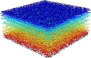
Magnetic density separation of end-of-life plastic is carried out by immersing a mixture of shredded plastic waste in a magnetically responsive liquid exposed to a magnetic field generated by properly designed magnets (Bakker et al. Reference Bakker, Rem and Fraunholcz2009; Hu Reference Hu2014; Luciani et al. Reference Luciani, Bonifazi, Rem and Serranti2015; Serranti et al. Reference Serranti, Luciani, Bonifazi, Hu and Rem2015). A continuous separation process is achieved by generating a flow of magnetic liquid through the magnetic field. Magnets used in MDS are designed such that the magnitude of the induced magnetic field has a gradient perpendicular to the flow direction and parallel to the gravitational force. This will cause the immersed particles to be sorted in different mass density fractions which are levitated at different heights. Once a mixture of particles is injected into the flow at the upstream end of the channel, sorted fractions can be recovered by employing separator plates mounted at different heights at the downstream end. Incorporating two magnets located at the top and bottom of the system enables separation of particles both lighter and heavier than the carrier liquid. A schematic of a typical MDS system for separation of waste plastic is shown in figure 1.

Figure 1. A schematic of a magnetic density separator. Different markers (colours) represent different mass densities.
Odenbach (Reference Odenbach1998) addressed the possibilities and challenges in the commercial use of MDS. In the design of an MDS system, one has to consider not only the properties of the magnetic field and the magnetic liquid, but also the interaction of the dispersed particles with the magnetofluidic system, and the interparticle interactions. The particle separation time, defined as the time required for all particles to reach their corresponding equilibrium positions is an important MDS design parameter. The shorter the particle separation time, the shorter will be the time required for the particles to be exposed to the magnetic field. Decreasing the particle separation time can lead to an increase in the throughput of particles and therefore, an increase in the efficiency of an MDS system. The particle separation time is in turn dependent on several parameters such as the particle size and shape, the magnetic fluid viscosity and its magnetization, and the external magnetic field. At appreciable volume fractions, the particle separation time can be increased due to the interparticle collisions.
The turbulence level in the separation channel is another crucial parameter in MDS (Hu Reference Hu2014). Maintaining a low level of turbulence in the separation channel is highly favourable, as turbulence level and mixing are intimately connected. A high turbulence level leads to an enhanced mixing, which can hamper the separation process. In new generations of MDS systems, measures have been taken to reduce the turbulence level in the separation chamber. These measures include the use of flow laminators such as honeycombs and screens at the upstream end of the separation channel and incorporation of moving walls (Serranti et al. Reference Serranti, Luciani, Bonifazi, Hu and Rem2015). The former decreases the upstream flow velocity fluctuations and vortices, and the latter aims to prevent the formation of boundary layers.
Design optimization of magnetic density separators requires a fundamental understanding of the collective motion of particles in a magnetic liquid. This requires the solution of many-particle problems that are coupled to a flow problem which is influenced by an external magnetic field. In this work, we present and employ a carefully chosen Euler–Lagrange approach to simulate the motion of particles in paramagnetic liquids.
Euler–Lagrange simulations are usually categorized into two families: particle-resolved simulations and point-particle simulations. Due to the prohibitively large computational resources required for particle-resolved simulations, we use a point-particle method, by incorporating appropriate models for forces and torques acting on the particles (Kuerten Reference Kuerten2016). The feedback forces and torques from particle to fluid are treated by introducing local source terms to the time-dependent incompressible Navier–Stokes equation of the fluid, which is solved with a pseudo-spectral method. We combine the point-particle approach with experimental observations to investigate the particle dynamics in paramagnetic liquids. The dynamics of a single particle as it moves towards its equilibrium position in a magnetic liquid is the basis for the behaviour of many-particle systems. A fundamental understanding of the motion of a single particle in a magnetic liquid is therefore crucial to understanding the collective motion of particles in larger magnetofluidic systems. Furthermore, the existence and stability of an equilibrium at which a particle is eventually levitated provides a useful framework for the investigation of particle motion in liquids within the Stokes regime (near the equilibrium point) and beyond it (farther from the equilibrium) where advective inertial forces are important. The motion of spherical and non-spherical particles in non-magnetic fluids has been the subject of several numerical and experimental investigations, see for instance Jenny, Dušek & Bouchet (Reference Jenny, Dušek and Bouchet2004), Horowitz & Williamson (Reference Horowitz and Williamson2010), Elghobashi & Truesdell (Reference Elghobashi and Truesdell1993) and Ern et al. (Reference Ern, Risso, Fabre and Magnaudet2012), but only a limited number of studies have addressed the dynamics of particles (drops) in magnetic liquids (Ueno, Higashitani & Kamiyama Reference Ueno, Higashitani and Kamiyama1995; Korlie et al. Reference Korlie, Mukherjee, Nita, Stevens, Trubatch and Yecko2008; Ghosh et al. Reference Ghosh, Gupta, Sahu, Das and Puri2020). When a particle is allowed to move freely under the combined effect of the magnetic buoyancy force and gravity, new features can occur in the particle motion. Singh, Das & Das (Reference Singh, Das and Das2018) used a one-fluid numerical model to explore the centre of mass and interface dynamics of an almost neutrally buoyant droplet (mass density ratio of  $1.15$) levitating in a ferrofluid. By approximating the vertical motion of the droplet by a simple dynamical model, the authors showed that depending on the parameters of the considered magnetofluidic set-up, the behaviour of vertical droplet motion can be monotonic or oscillating.
In the present work, we combine experimental observations with numerical simulations to investigate the motion of rigid non-magnetic spherical particles within the particle-to-fluid mass density ratio range  $[0.7,1.3]$ in a paramagnetic liquid. Our numerical model employs a four-way coupled point-particle approach to represent both the fluid flow and the motion of the inertial particles. The aim of this paper is three-fold. First, the one-dimensional dynamics of a single spherical particle moving in a paramagnetic liquid exposed to a magnetic field gradient is addressed. Through a priori mathematical analysis, the nature of the motion of a single spherical particle in a paramagnetic liquid is parameterized. Solutions of the governing equation of the translational motion of a spherical particle in a paramagnetic liquid are compared with experimental observations. Second, the effect of collisions in two-particle systems is investigated. We validate our numerical model by comparison with results of PTV experiments in one- and two-particle systems. Finally, many-particle systems are numerically studied. Parametric studies are performed to investigate the effect of the incorporation of the Basset history force, two-way coupling and collisions in a practical MDS case. Next, the effect of particle size and initial particle distribution on the separation efficiency is investigated.
The rest of the paper is organized as follows. We introduce the mathematical model for the problem in § 2. With an introduction to the hydrodynamics of magnetically responsive liquids in § 3, we address the concept of apparent mass density and buoyancy force in magnetic liquids. Different elements of the model, including the magnetic field, magnetic liquid and the immersed particles are discussed. The numerical solution approach and the experimental set-up are described in §§ 3 and 4, respectively. In § 5 first, the vertical motion of an individual spherical particle in a magnetic liquid is parameterized. Next, the numerical results are validated against experimental observations in single- and two-particle systems. Finally, the separation performance of many-particle systems is investigated numerically. Concluding remarks and future directions are addressed in § 6.
2. Mathematical description
In this section, we present the mathematical model for the incompressible isothermal flow of a magnetically responsive fluid laden with spherical particles. The considered system consists of three elements: a magnetic liquid considered as a continuous phase which is described by an Eulerian approach, discrete particles which are described in a Lagrangian way, and a steady external magnetic field. The immersed non-magnetic particles in the magnetized liquid are assumed to be rigid spheres which interact with each other through collisions. The discrete particles and the continuous phase are coupled by means of two-way momentum transfer. The particles are modelled as point particles, and the interaction between fluid and particles is modelled by using correlations for all relevant forces and torques. For the equation of motion of the magnetic liquid, we follow the quasi-equilibrium theory of Rosensweig (Reference Rosensweig2013), where fluid magnetization is assumed to be in local equilibrium with the magnetic field, and  $\boldsymbol {M} \times \boldsymbol {H}=0$, where
  $\boldsymbol {H}$ is the magnetic field vector and
  $\boldsymbol {M}$ is the fluid magnetization vector. This assumption is valid for paramagnetic salt solutions. In such liquids, due to the small size of magnetized fluid elements (ionized molecules), the coupling between the magnetic and mechanical degrees of freedom of the molecules is very small, and the magnetization relaxation to the direction of
  $\boldsymbol {H}$ is almost instantaneous (Shliomis Reference Shliomis and Odenbach2002).
We first introduce the governing equations of motion of a paramagnetic liquid exposed to a magnetic field gradient in § 2.1. In § 2.2, the magnetic fields considered in this study are presented. Spherical non-magnetic particles moving in a paramagnetic liquid experience various static and dynamic forces. In § 2.3 we discuss the buoyancy force in a magnetized liquid as the driving force for the particle levitation motion, and introduce the concept of apparent mass density. The equations describing the motion of particles in a paramagnetic liquid are presented in § 2.4, where all relevant fluid–particle interaction mechanisms are addressed.
2.1. Continuous phase
The motion of a magnetically responsive fluid in a magnetic field is influenced by a Kelvin body force which arises from the interaction between the local magnetic field and the molecular magnetic moments characterized by the fluid magnetization. This force is in addition to the gravitational body force acting on the fluid. Under the assumption of equilibrium magnetization, the governing equations of the incompressible flow of a Newtonian magnetically responsive fluid can be written as (Rosensweig Reference Rosensweig2013)
 \begin{gather} \rho_{f}\left(\frac{\partial \boldsymbol{u}}{\partial t} + (\boldsymbol{u} \boldsymbol{\cdot} \boldsymbol{\nabla}) \boldsymbol{u}\right)= -\boldsymbol{\nabla}p^ *+\mu\nabla^2 \boldsymbol{u}+ \mathfrak{F}^{inter},\end{gather}
 \begin{gather} \boldsymbol{\nabla} \boldsymbol{\cdot} \boldsymbol{u} =0, \end{gather}
where  $\boldsymbol {u}$ denotes the fluid velocity,
  $\mu$ is the dynamic viscosity of the fluid and
  ${\rho _{f}}$ is the mass density of the fluid. Here
  $p^*$ represents a reduced pressure which accounts for the effects of the gravitational and the magnetic body forces. With gravity acting in the direction of
  $-\boldsymbol {e}_y$, this reduced pressure is defined as
 \begin{equation} p^*=p-p_{static} =p+{\rho_{f}}g{y}-{\mu_0} \int_{0}^{H} M\,\textrm{d}H, \end{equation}
where  $M=|\boldsymbol {M}|$ is the magnitude of the fluid magnetization,
  $H=|\boldsymbol {H}|$ is the magnetic field strength and
  $\mu _{0}$ denotes the permeability of vacuum. The term
  $\mathfrak {F}^{inter}$ in (2.1) is the fluid–particle coupling term which takes care of the momentum transfer from the discrete particles to the fluid. The flow field is obtained by solving (2.1) and (2.2) in a cubic domain with dimensions
  $L_x \times L_y \times L_z$, where
  $x$,
$x$,  $y$ and
  $z$ denote the streamwise, wall-normal and spanwise directions, respectively.
The magnetic liquid considered in this study is an aqueous paramagnetic fluid ( $\textrm {MnCl}_2$ salt solution) with a linear magnetization behaviour (Rosensweig Reference Rosensweig2013). If we let
  $\chi$ denote the magnetic susceptibility of the liquid, the magnetization vector field is defined as
 \begin{equation} \boldsymbol{M}=\chi \boldsymbol{H}. \end{equation}
Both magnetic susceptibility and dynamic viscosity of paramagnetic salt solutions are dependent on the concentration of the solution (Andres Reference Andres1976).
2.2. Magnetic field
In this work, we consider one-dimensional magnetic fields which are uniform in planes parallel to the surface of the magnet ( ${\partial H}/{\partial x}={\partial H}/{\partial z}= 0$), and decay exponentially with the vertical distance from the magnet surface. Such magnetic fields can be generated by incorporating a specially designed array of alternately rotating magnetic poles (Shute et al. Reference Shute, Mallinson, Wilton and Mapps2000; Fernow Reference Fernow2016; Polinder & Rem Reference Polinder and Rem2017). In the regions sufficiently far from the magnet edges, the generated magnetic field by such configurations closely follows
 \begin{equation} \boldsymbol{H}=H(y)\boldsymbol{e}_y. \end{equation}
For a magnet located at the bottom of the computational domain such that its upper surface is located at  $y=-L$, the magnetic field strength reads
 \begin{equation} H (y)= H_0\textrm{e}^{-{\rm \pi} (L+y)/p}, \quad y \in [-L,\infty], \end{equation}
where  $H_0$ is the magnetic field strength at the surface of the magnet and
  $p$ denotes the pole size. Expression (2.6) is the solution of the Maxwell equation on the strong side of an infinitely long Halbach array with continuously varying magnetization (Halbach Reference Halbach1981). The reader is referred to Mallinson (Reference Mallinson1973) for the derivation. If the magnet is located at the top of the computational domain with its lower (strong) surface at
  $y=+L$, the magnetic field strength follows
 \begin{equation} H (y)= H_0\textrm{e}^{-{\rm \pi} (L-y)/p}, \quad y \in [-\infty,L]. \end{equation}
In the case where two identical magnets are located at the top and bottom of the computational domain with their strong sides facing each other, the magnitude of the magnetic field is assumed to be a linear superposition of the magnetic fields corresponding to each magnet, as follows:
 \begin{equation} H (y)=H_0 \left(\textrm{e}^{-{\rm \pi} (L+y)/p}+\textrm{e}^{-{\rm \pi} (L-y)/p}\right), \quad y \in [-L,L]. \end{equation}
For the sake of simplicity, in § 3 we consider a one-magnet configuration with a magnet located at the bottom of the domain and its magnetic field strength following (2.6). For simulations of many-particle systems discussed in § 4, a two-magnet configuration with a magnetic field strength given by (2.8) is considered.
2.3. Buoyancy in magnetic liquids
Let us now consider a situation when a non-magnetic body with volume  $V_i$ is immersed in a magnetic liquid exposed to an arbitrary magnetic field, as shown in figure 2.The buoyancy force acting on the body can be calculated by applying the Gauss divergence theorem to the surface integral of the static pressure at the interface
  $s$, as follows:
 \begin{align} \boldsymbol{F}_{B} &=-\int_{s} p_{static} {\boldsymbol{n}}\,\mathrm{d} s=-\int_{V_i} \boldsymbol{\nabla} p_{static}\,\mathrm{d} V\nonumber\\ &\quad =\int_{V_i}(\rho_{f} g\boldsymbol{e}_y-\mu_0M \boldsymbol{\nabla} H) \,\mathrm{d} V. \end{align}
Under the assumption of a constant magnetic force within the volume of the immersed body (small body), the term  $M\boldsymbol {\nabla } H$ can be assumed to be constant within the volume
  $V_i$, and the buoyancy force can be approximated by
 \begin{equation} \boldsymbol{F}_{{B},i} \approx \rho_{f}V_i g\boldsymbol{e}_y- \mu_0{V_i} {M} \boldsymbol{\nabla} {H}. \end{equation}
The first term in (2.10) is the conventional gravitational buoyancy force (also known as the Archimedes force) which is constant throughout the liquid. The second term is the magnetic contribution to the buoyancy force we refer to as the ‘magnetic buoyancy force’. If the magnets are designed such that the magnetic field gradient is parallel to the gravitational force, the combined magnetic and gravitational buoyancy force reads
 \begin{equation} \boldsymbol{F}_{{B},i}\approx \left(\rho_{f}g- \mu_0 {M} \frac{\textrm{d}H}{\textrm{d}y}\right)\boldsymbol{V}_i\boldsymbol{e}_y={\rho_{f,a}} V_ig\boldsymbol{e}_y, \end{equation}
where
 \begin{equation} \rho_{f,a} \approx \rho_{f}- \left(\frac{\mu_0}{g} \right)M\frac{\textrm{d}H}{\textrm{d}y} \end{equation}
is denoted as the ‘apparent fluid mass density’. If it exists, the equilibrium position of an immersed body is the position where the magnitude of the total buoyancy force is equal to the magnitude of the opposing gravitational body force acting on the body. At this position, the local apparent mass density of the fluid is equal to the mass density of the body. For a fixed magnetofluidic system, the equilibrium position of a body is only dependent on its mass density. Therefore, by a careful adjustment of the magnetic field and the magnetic fluid properties, a gradient of apparent mass density can be generated wherein particles in a specific mass density range can be separated.

Figure 2. A particle immersed in a magnetic liquid exposed to a magnetic field gradient.
The apparent mass density profile of a paramagnetic liquid exposed to a magnetic field of a bottom-magnet system given by (2.6) reads
 \begin{equation} \rho_{f,a} =\rho_{f} +\frac{{\rm \pi}\mu_0 \chi H_0^2}{pg} \exp\left({\frac{-2{\rm \pi} (L+y)}{p}}\right). \end{equation}
For a top-magnet configuration where the magnetic field follows (2.7) apparent fluid mass density is
 \begin{equation} \rho_{f,a} =\rho_{f} -\frac{{\rm \pi}\mu_0 \chi H_0^2}{pg}\exp\left({\frac{-2{\rm \pi} (L-y)}{p}}\right) \end{equation}
and for a two-magnet configuration with a magnetic field given by (2.8), the apparent mass density of the liquid reads
 \begin{equation} \rho_{f,a} =\rho_{f} -\frac{2{\rm \pi}\mu_0 \chi H_0^2}{pg} \exp\left({-\frac{2{\rm \pi} L}{p}}\right)\sinh\left(\frac{2{\rm \pi} y}{p}\right). \end{equation}
It follows directly from (2.13) and (2.14) that the maximum change in the apparent mass density of the fluid for a one-magnet system is
 \begin{equation} |\Delta \rho_{f,a}|_{max} = |\rho_{f,a}- \rho_{f}|_{max}=\frac{{\rm \pi}\mu_0 \chi H_0^2}{pg}, \end{equation}
and from (2.15), for a two-magnet configuration,
 \begin{equation} |\Delta \rho_{f,a}|_{max} = |\rho_{f,a}- \rho_{f}|_{max}=\frac{{\rm \pi}\mu_0 \chi H_0^2}{pg}\left|1-\exp\left({\frac{-4{\rm \pi} L}{p}}\right)\right|. \end{equation}
The local gradient of the apparent mass density in the magnetic liquid is an indication of the separation resolution in an MDS system, as it determines the local separation distance of two consecutive mass density groups. The maximum gradient of apparent mass density for a one-magnet system is
 \begin{equation} \max \left(\frac{\textrm{d}\rho_{f,a}}{\textrm{d}y}\right) = \frac{2 {\rm \pi}^2\mu_0 \chi H_0^2}{{p}^2g}. \end{equation}
For a two-magnet configuration, the maximum gradient of apparent mass density is
 \begin{equation} \max \left(\frac{\textrm{d}\rho_{f,a}}{\textrm{d}y}\right) = \frac{4 {\rm \pi}^2\mu_0 \chi H_0^2}{{p}^2g} \left(1+\exp\left({\frac{-4 {\rm \pi}L}{p} }\right)\right). \end{equation}
2.4. Particle phase
2.4.1. Equation of motion
The motion of rigid spherical particles immersed in a magnetically responsive liquid is described by solving the translational and rotational equations of motion for each particle where contributions from various fluid–solid interaction mechanisms are taken into account. The translational motion of particles is based on an extension of the equation of motion derived by Maxey & Riley (Reference Maxey and Riley1983). It is well known that for almost neutrally buoyant particles the contributions of the Basset history force, the added mass force and the force due to the undisturbed velocity field to the motion of the particle cannot be neglected (Kuerten Reference Kuerten2016). The included forces in the Maxey–Riley equation are the force due to the undisturbed velocity field,  $\boldsymbol {F}_{{U},i}$, steady viscous drag force,
  $\boldsymbol {F}_{{D},i}$, added mass force,
  $\boldsymbol {F}_{{AM},i}$, history force,
  $\boldsymbol {F}_{{H},i}$, gravitational body force,
  $\boldsymbol {F}_{{G},i}$, and the buoyancy force,
  $\boldsymbol {F}_{{B},i}$.
For the drag coefficient, we consider the widely used correlation of Schiller & Naumann (Reference Schiller and Naumann1933) for a non-creeping flow. The history force correction to the drag is based on the classic Basset kernel; although correlations for history force for non-creeping flows are derived (Kim, Elghobashi & Sirignano Reference Kim, Elghobashi and Sirignano1998). In this work, we neglect the finite Reynolds number effects on the history kernel. The Faxén corrections for non-uniform flows and the lift force are not considered here as the background flow is assumed to be uniform.
The trajectory of each particle is obtained by solving the following set of differential equations:
 \begin{gather} \frac{\textrm{d} \boldsymbol{x}_i}{\textrm{d}t} = \boldsymbol{v}_i, \end{gather}
 \begin{gather}\frac{\textrm{d} \boldsymbol{v}_i}{\textrm{d}t} =\frac{1}{m_i}\left(\sum \boldsymbol{F}_i+\boldsymbol{F}^{(c)}_i\right), \end{gather}
with
 \begin{align} \sum \boldsymbol{F}_i&=\underbrace{\rho_{{f}} V_i\frac{\textrm{D} \boldsymbol{u}_{i}}{\textrm{D} t}}_{\boldsymbol{F}_{{U},i}}+\underbrace{\rho_{{p},i}V_i \frac{\left(\boldsymbol{u}_i-\boldsymbol{v}_{i}\right)}{\tau_{{t},i}}\left(1+0.15 Re_{{t},i}^{0.687}\right)}_{\boldsymbol{F}_{{D},i}}\nonumber\\ &\quad +\underbrace{\frac{3}{2}\left({\rm \pi} \rho_{f} \mu\right)^{1 / 2} d_{p}^{2}\left[\int_{-\infty}^{t} \frac{\dfrac{\textrm{d}}{\textrm{d}\tau}\left(\boldsymbol{u}_{i}-\boldsymbol{v}_{i}\right)}{(t-\tau)^{1 / 2}}\,\textrm{d}\tau\right]}_{\boldsymbol{F}_{{H},i}}\nonumber\\ &\quad +\underbrace{\frac{1}{2}\rho_{{f}} V_i\left(\frac{\textrm{D} \boldsymbol{u}_i}{\textrm{D} t}-\frac{\textrm{d} \boldsymbol{v}_i}{\textrm{d} t}\right)}_{\boldsymbol{F}_{{AM},i}}-\underbrace{\rho_{{p},i}V_i g\boldsymbol{e}_y}_{\boldsymbol{F}_{{G},i}}+\underbrace{\rho_{f,a}V_i g\boldsymbol{e}_y}_{\boldsymbol{F}_{{B},i}}, \end{align}
where  $Re_{{t},i}=d_{p}|\boldsymbol {u}_i-\boldsymbol {v}_i|/\nu$ denotes the particle translational Reynolds number,
  $\boldsymbol {v}_i$ is the particle translational velocity and
  $\boldsymbol {u}_i$ is the undisturbed fluid velocity at the position of the particle. Here
  $\tau _{{t},i}=\rho _{p}d_{p}^2/18 \mu$ is the particle translational relaxation time and
  $\boldsymbol {F}^{(c)}_i$ represents the force on a particle due to a collision with another particle or a wall.
Special care must be taken in evaluating the Basset history term when the relative particle–fluid velocity undergoes a step change. The derivation of the Basset history force is based on the assumption that the particle is present in the fluid at all times. The case where the initial particle velocity is not equal to the initial fluid velocity at the position of the particle is equivalent to the case where the particle is in a stagnant fluid for  $t\in (-\infty ,0)$ and the fluid velocity undergoes a step change at
  $t=0$ (Kim et al. Reference Kim, Elghobashi and Sirignano1998). Under such circumstance, the Basset integral can be written as
 \begin{align} \int_{-\infty}^{t} \frac{\dfrac{\textrm{d}}{\textrm{d} \tau}\left(\boldsymbol{u}_{i}-\boldsymbol{v}_{i}\right)}{(t-\tau)^{1 / 2}}\,\textrm{d}\tau = \int_{t_s^+}^{t} \frac{\dfrac{\textrm{d}}{\textrm{d} \tau}\left(\boldsymbol{u}_{i}-\boldsymbol{v}_{i}\right)}{(t-\tau)^{1 / 2}}\,\textrm{d} \tau +\frac{\boldsymbol{u}_{i}(t_s^+)-\boldsymbol{v}_{i}(t_s^+)-\boldsymbol{u}_{i}(t_s^-)+\boldsymbol{v}_{i}(t_s^-)}{(t-t_s)^{1/2}}, \end{align}
where  $t_s=\max \{0,t_c\}$ is the time at which the step change occurs. A step change can occur in simulations with non-zero velocity difference between the particle and the fluid at
  $t=0$, or during a particle–particle or particle–wall collision at
  $t=t_c$. The second term on the right-hand side of (2.23) is associated with such step changes in the particle–fluid relative velocity. At a collision instance,
  $t_c$, the post-collision history integral can be written as
 \begin{align} \int_{-\infty}^{t} \frac{\dfrac{\textrm{d}}{\textrm{d} \tau}\left(\boldsymbol{u}_{i}-\boldsymbol{v}_{i}\right)}{(t-\tau)^{1 / 2}}\,\textrm{d} \tau = \int_{t_c^+}^{t} \frac{\dfrac{\textrm{d}}{\textrm{d} \tau}\left(\boldsymbol{u}_{i}-\boldsymbol{v}_{i}\right)}{(t-\tau)^{1 / 2}}\,\textrm{d}\tau +\frac{\boldsymbol{u}_{i}(t_c^+)-\boldsymbol{v}_{i}(t_c^+)-\boldsymbol{u}_{i}(t_c^-)+\boldsymbol{v}_{i}(t_c^-)}{(t-t_c)^{1/2}}. \end{align}
Under the assumption of an infinitesimally small collision duration, the fluid velocity remains constant;  $\boldsymbol {u}_{i}(t_c^-)=\boldsymbol {u}_{i}(t_c^+)$. After each collision, the Basset integral (the precollision history) can be set to zero and the post-collision Basset history can be calculated as
 \begin{equation} F_h = \frac{3}{2}\left({\rm \pi} \rho_{f} \mu\right)^{1 / 2} d_{i}^{2}\left[ \int_{t_c}^{t} \frac{\dfrac{\textrm{d}}{\textrm{d}\tau}\left(\boldsymbol{u}_{i}-\boldsymbol{v}_{i}\right)}{(t-\tau)^{1 / 2}}\,\textrm{d}\tau +\frac{\boldsymbol{v}_{i}(t_c^-)-\boldsymbol{v}_{i}(t_c^+)}{(t-t_c)^{1/2}}\right]. \end{equation}
Inclusion of the Basset history force in (2.22) presents a numerical difficulty which mainly arises from the need to store the relative particle acceleration over the entire history of particle motion. Section 3 addresses the employed numerical approximation to overcome this difficulty.
The rotational motion of the dispersed phase is based on the theoretical equation of Dennis, Singh & Ingham (Reference Dennis, Singh and Ingham1980) for the steady viscous torque against particle rotation. The angular velocity of the particles is obtained by solving
 \begin{equation} \frac{\textrm{d}\boldsymbol{\varOmega}_i}{\textrm{d}t} =\frac{1}{I_i}\left(\boldsymbol{T}_i+\boldsymbol{T}^{(c)}_i\right), \end{equation}
where
 \begin{equation} {\boldsymbol{T}_i} = -C_{T} \frac{1}{2} \rho_{p}\left(\frac{{d}_{p}}{2}\right)^{5}\left|\frac{1}{2}\boldsymbol{\omega}_{i} -\boldsymbol{\varOmega}_i\right| \left(\frac{1}{2}\boldsymbol{\omega}_{i}-\boldsymbol\varOmega_{i}\right), \end{equation}
with
 \begin{equation} C_{T}=\left\{\begin{array}{@{}ll} \dfrac{64 {\rm \pi}}{{Re}_{r,i}}, & \text{if}\ {Re}_{r,i}\leq 32,\\ \dfrac{12.9}{\sqrt{{Re}_{r,i}}}+\dfrac{128.4}{{Re}_{r,i}} & \text{if}\ 32<{Re}_{r,i}<1000, \end{array} \right. \end{equation}
where  $Re_{r,i}=d_{p}^{2}|(\boldsymbol {\omega }_{i}-\boldsymbol {\varOmega }_{i})/2|/\nu$ is the rotational Reynolds number,
  $\boldsymbol {\varOmega }_i$ represents the particle angular velocity,
  $\boldsymbol {\omega }_i$ is the undisturbed fluid vorticity at the position of the particle, and
  $I_i={2}(m_i(d_{p}/2)^2)/5$ is the moment of inertia. Here
  $\boldsymbol {T}^{(c)}_i$ is the torque on a particle due to a collision with a particle or a wall. It should be noted that considering the low particle volume fraction (maximum
  $0.02$) in the cases addressed in this study, the torque coupling between the particles and the liquid is assumed to be one-way, i.e. the feedback torque on the liquid is neglected.
2.4.2. Collisions
The interparticle and particle–wall interactions are treated by a hard-sphere collision model which closely follows the method of Hoomans et al. (Reference Hoomans, Kuipers, Briels and van Swaaij1996). The collision time is assumed to be infinitesimally small, and the precollision and post-collision translational and angular velocities are explicitly related through normal and tangential restitution coefficients and a dynamic friction factor. Consider two colliding particles with centre position vectors  $\boldsymbol {x}_a$ and
  $\boldsymbol {x}_b$ and contact point
  $c$. The normal unit vector at the contact point
  $c$ is
 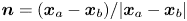 $\boldsymbol {n}=(\boldsymbol {x}_a-\boldsymbol {x}_b)/|\boldsymbol {x}_a-\boldsymbol {x}_b|$. If we let the superscripts
  $+$ and
  $-$ represent the post-collision and precollision properties, respectively, the tangential unit vector at the contact point is
  $\boldsymbol {t}=(\boldsymbol {v}_{ab}^--\boldsymbol {n}(\boldsymbol {v}_{ab}^- \boldsymbol {\cdot } \boldsymbol {n}))/|\boldsymbol {v}_{ab}^--\boldsymbol {n}(\boldsymbol {v}_{ab}^- \boldsymbol {\cdot } \boldsymbol {n})|$, where
 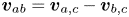 $\boldsymbol {v}_{ab}=\boldsymbol {v}_{a,c}-\boldsymbol {v}_{b,c}$ is the particle relative velocity at the contact point. The post-collision translational and rotational velocities can be derived according to the following equations:
 \begin{equation} \left. \begin{gathered} m_{a}\left(\boldsymbol{v}_{a}^+-\boldsymbol{v}_{a}^-\right) =-m_{b}\left(\boldsymbol{v}_{b}^--\boldsymbol{v}_{b}^+\right)=\boldsymbol{J},\\ \frac{I_{a}}{R_{a}}\left(\boldsymbol{\omega}_{a}^+-\boldsymbol{\omega}_{a}^-\right) =\frac{I_{b}}{R_{b}}\left(\boldsymbol{\omega}_{b}^+-\boldsymbol{\omega}_{b}^-\right)=-\boldsymbol{n} \times \boldsymbol{J}, \end{gathered} \right\} \end{equation}
where  $R=d_{p}/2$ is the particle radius,
  $m$ is the particle mass and
  $\boldsymbol {J}$ is the impulse vector. The normal component of the impulse vector is given by
 \begin{equation} J_{n}=-(1+e_{n,{eff}}) m_{a b} \boldsymbol{v}_{a b}^- \boldsymbol{\cdot} \boldsymbol{n}, \end{equation}
where  $e_{n,{eff}}=-\boldsymbol {v}_{a b}^- \boldsymbol {\cdot } \boldsymbol {n}/\boldsymbol {v}_{a b}^+ \boldsymbol {\cdot } \boldsymbol {n}$ denotes the effective coefficient of normal restitution, and
  $m_{ab}$ is the reduced mass defined as
 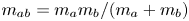 $m_{a b}= m_am_b/(m_a+m_b)$. For the tangential component of the impulse vector a distinction can be made based on the type of collision being either ‘sticking’ or ‘sliding’, as follows:
 \begin{align} J_{t}=\left\{\begin{array}{@{}ll} {-\dfrac{2}{7}\left(1+e_{t,{eff}}\right) m_{a b} \boldsymbol{v}_{a b, 0} \boldsymbol{\cdot} \boldsymbol{t}} & \text{if}\ \mu_{f} J_{n} \geq \dfrac{2}{7}\left(1+e_{t,{eff}}\right) m_{a b} \boldsymbol{v}_{a b, 0} \boldsymbol{\cdot} \boldsymbol{t} \ {(\textrm{stick})},\\ {-\mu_{f} J_{n}} & \text{otherwise} \ {(\textrm{slide})}, \end{array} \right. \end{align}
where 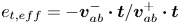 $e_{t,{eff}}= -\boldsymbol {v}_{a b}^- \boldsymbol {\cdot } \boldsymbol {t}/\boldsymbol {v}_{a b}^+ \boldsymbol {\cdot } \boldsymbol {t}$ is the effective coefficient of tangential restitution and
  $\mu _{ f}$ is the coefficient of dynamic friction.
From the modelling viewpoint, appropriate values for the coefficients of restitution and friction coefficient are of great importance in the prediction of the post-collision dynamics. When interparticle or particle–wall collisions occur in the absence of a viscous fluid (dry collisions), the kinetic energy of the particles is dissipated purely due to the contact mechanism. In a viscous fluid, however, the collision process is influenced by the viscous and inertial interactions of the particle with the fluid. To account for the hydrodynamic effects of the surrounding fluid on the normal component of motion during a collision, an effective coefficient of normal restitution is introduced (Davis, Serayssol & Hinch Reference Davis, Serayssol and Hinch1986; Gondret, Lance & Petit Reference Gondret, Lance and Petit2002). The normal component of post-collision velocity of particles during a non-head-on collision follows the behaviour of a head-on collision (Yang & Hunt Reference Yang and Hunt2006). Regardless of the type of collision (oblique or head-on), the effective (wet) normal coefficient of restitution increases with the binary normal Stokes number defined as
 \begin{equation} St_{n}=\frac{2}{9}\frac{\rho_{p}^*}{\rho_{f}}{Re_{rel}}, \end{equation}
where 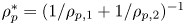 $\rho _{p}^*=(1/\rho _{p,1}+1/\rho _{p,2})^{-1}$ is a reduced particle mass density, and
 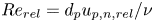 $Re_{rel}=d_{p} u_{{p},n,{rel}}/ \nu$ denotes the relative Reynolds number based on the normal component of the particle relative velocity
  $u_{{p},n,{rel}}$. Izard, Bonometti & Lacaze (Reference Izard, Bonometti and Lacaze2014) proposed a model which can capture the experimentally observed effective coefficient of normal restitution for the range of Stokes number
  $0<St_{n}< 10^6$. This correlation relates the effective normal coefficient of restitution to the corresponding dry coefficient, the Stokes number, and the effective particle roughness height. For a particle–particle collision this correlation reads
 \begin{equation} \frac{e_{n,{eff}}}{e_{n,{dry}}}=\left(1+\frac{1}{St_{n}} \ln \left(\frac{2\eta_{e}}{d_{p}}\right)\right) \exp \left(-\frac{{\rm \pi} / 2}{\sqrt{St_n+\ln \left(\dfrac{2\eta_{e}}{d_{p}}\right)}}\right), \end{equation}
where  $\eta _e$ is an effective average particle surface roughness height. The qualitative behaviour of immersed oblique collisions is similar to that of dry collisions. The effective values for coefficients of dynamic friction and tangential restitution depend on the considered fluid–particle system and the relative velocity of the particles (Joseph & Hunt Reference Joseph and Hunt2004). According to Walton's hard-sphere model (Walton Reference Walton1993), the dynamic friction coefficient and the tangential coefficient of restitution can be obtained by plotting the tangent of rebound angle as a function of tangent of incidence angle. These two tangents are given by
 \begin{equation} \left. \begin{gathered} \varPsi_{{in}}=\frac{\left(\boldsymbol{v}_{a b}^+ \boldsymbol{\cdot} \boldsymbol{t}\right)}{\left(\boldsymbol{v}_{a b}^- \boldsymbol{\cdot} \boldsymbol{n}\right)},\\ \varPsi_{{out}}=\frac{\left(\boldsymbol{v}_{a b}^- \boldsymbol{\cdot} \boldsymbol{t}\right)}{\left(\boldsymbol{v}_{a b}^- \boldsymbol{\cdot} \boldsymbol{n}\right)}, \end{gathered} \right\} \end{equation}
for the sticking collisions,  $\varPsi _{{out}}= -e_{t,{eff}}\varPsi _{{in}}$, and for sliding collisions,
  $\varPsi _{{out}}= \varPsi _{{in}}-({7}/{2})\mu _{eff}(1+e_{n,{eff}})$. In a similar manner, in § 5.2.2 we will determine the effective (lubricated) dynamic friction coefficient,
  $\mu _{eff}$, and effective coefficient of tangential restitution,
  $e_{{t,eff}}$, by performing several particle–particle collision experiments at different incidence angles.
3. Numerical approach
3.1. Fluid phase
The flow field is obtained by reducing (2.1) and (2.2) to a fourth-order equation for wall-normal velocity component and a second-order equation for the wall-normal component of vorticity. The equations are discretized in space by using a pseudo-spectral method. Our method incorporates a Fourier–Galerkin approach in the periodic directions,  $x$ and
  $z$, and a Chebyshev-tau method in the wall-normal direction,
  $y$. The temporal discretization of the linear terms is carried out by a three-stage Runge–Kutta scheme, and the nonlinear terms are advanced in time by the Crank-Nicolson method. For details of the numerical approach, the reader is referred to Kuerten, Van der Geld & Geurts (Reference Kuerten, Van der Geld and Geurts2011).
3.2. Particle phase
3.2.1. Time integration
The equations of translational and rotational motion of spherical particles (2.20), (2.21) and (2.26) are discretized in time using a forward Euler method. Our explicit scheme takes the partial time step of each stage of the Runge–Kutta scheme used for the fluid solver as a time step.
In the numerical solution of system (2.22), integration of the Basset history term is the most time-consuming. To decrease the numerical costs of the evaluation of the Basset history contribution, we use the method of Van Hinsberg, ten Thije Boonkkamp & Clercx (Reference Van Hinsberg, ten Thije Boonkkamp and Clercx2011) where a ‘window’ is applied to the Basset kernel. The history kernel is split into a window kernel and a tail kernel. The window kernel (recent history) is approximated by an ordinary trapezoidal rule over the interval  $[t-t_{win},t]$ that consists of the
  $N_{w}$ previous time steps. The tail kernel (old history) over the time interval
  $(-\infty , t-t_{win})$ is approximated by a sum of exponential functions, leading to a considerable reduction in computational time as well as in memory requirements.
3.3. Two-way coupling: fluid–particle momentum transfer
The presence of particles in the fluid is represented by a local feedback force from the particles on the fluid defined as
 \begin{equation} \mathfrak{F}^{{ inter }}(\boldsymbol{x}) \equiv -\sum_{n=1}^{N_{p}} \mathcal{P}\left(\boldsymbol{x}-\boldsymbol{x}_{p}^{(n)}\right) \boldsymbol{F}_{{2w}}^{(n)}, \end{equation}
where  $N_{p}$ is the total number of particles and
  $\boldsymbol {F}_{{2w}}^{(n)}$ is the feedback force from the
  $n\textrm {th}$ particle modelled as
 \begin{equation} \boldsymbol{F}_{{2w}}^{(n)}=\boldsymbol{F}_{{U}}+\boldsymbol{F}_{{D}}+\boldsymbol{F}_{{H}}+\boldsymbol{F}_{{AM}}. \end{equation}
In point-particle Euler–Lagrange simulations the term  $\mathcal {P}(\boldsymbol {x}-\boldsymbol {x}_{p}^{(n)})$ is usually a numerical projection of the Dirac delta function from the particle centre
  $\boldsymbol {x}_{{p}}^{(n)}$ to the Eulerian grid point
  $\boldsymbol {x}$. A common approach to numerical projection
  $\mathcal {P}$ is to distribute the feedback force over the eight grid points surrounding the particle centre using the same weights as for the interpolation of fluid properties to the position of the particle (point-force approach). In the limit of particles which are much smaller than the size of the Eulerian grid spacing, this approach is theoretically valid. However, as the particle size approaches the size of the grid spacing, the feedback force to the fluid momentum equation is spread over a volume. Since in our simulations the grid size can be smaller than the particle diameter
  $d_{p}$, we choose to distribute the particle feedback force over a volume approximately equal to the volume of the particle. A top-hat filter is implemented to distribute the feedback force from the Lagrangian particle position to the Eulerian grid points, as follows:
 \begin{equation} \mathcal{P}(\boldsymbol{x}-\boldsymbol{x}_{p})= \begin{cases} \dfrac{1}{\sigma_{1}\sigma_{2}\sigma_{3}}, & \text{if } \left|x_{k}-x_{{p},k}\right|<\sigma_k / 2 \ (k=1,2,3),\\ 0, & \text{otherwise.} \end{cases} \end{equation}
The width of the filter  $\sigma _k$,
  $k=1,2,3$ is closest to the width of the particle encompassing cube in each direction. This means that the particle feedback force is distributed over a rectangular block with a volume closest to the volume of the smallest bounding box around the particle. This allows us to keep the feedback force distribution volume constant under mesh refinement. Furthermore, considering the fact that the grid spacing is not uniform in the wall-normal direction, the distribution volume is independent of the local grid spacing. Figure 3 shows a schematic of the applied filter for several particle positions.

Figure 3. A two-dimensional schematic of the top-hat filter used to distribute the feedback force from the Eulerian particle position to the Eulerian grid points. Here  $\sigma _1$ and
  $\sigma _2$ are widths of the filter in the
  $x$- and
  $y$-directions, respectively.
4. Experimental set-up
We validate the results of our numerical approach with experimentally obtained particle tracks in single- and two-particle systems. For this purpose, an experimental set-up is designed which enables the investigation of levitation motion of single spherical particles, as well as binary collision dynamics in a paramagnetic liquid subject to a magnetic field gradient. The paramagnetic liquid is synthesized by dissolving solid  $\textrm {MnCl}_2$ salt in distilled water up to the saturation point. The solution is afterwards filtered twice with filters of pore sizes
  $3\ \mathrm {\mu }\textrm {m}$ and
  $1\ \mathrm {\mu }\textrm {m}$, and is stabilized by hydrochloric acid. The molality of the final aqueous solution is
  $4.62\ \textrm {mol}\,\textrm {kg}^{-1}$.
Measurements are performed in a  $15\ \textrm {cm}\times 15\ \textrm {cm} \times 15\ \textrm {cm}$ cubic tank. The particles can be inserted either at the top or through a hole at the bottom of the tank. A magnet is located underneath the tank to generate the desired magnetic field in the form of (2.6). The magnet is designed such that the induced magnetic field has a vertical gradient at the centre of the tank, where the measurements are performed. Two cameras are used to record the particle trajectories through two perpendicular sidewalls of the tank by means of three-dimensional PTV. A schematic of the experimental set-up is shown in figure 4(a). The particles considered for the experiments are spherical unplasticized polytetrafluorethylene (PVC-U) and polyoxymethylene (POM) beads with mass densities
  $\rho _{{{p}},1}=1434\ \textrm {kg}\,\textrm {m}^{-3}$ and
  $\rho _{{{p}},2}=1406\ \textrm {kg}\,\textrm {m}^{-3}$, respectively. Some of the experimental parameters are summarized in table 1. Figure 4(b) depicts the magnetic field strength on the vertical line passing through the centre of the tank, which is measured using a Gauss meter. An exponential function of the form of (2.6) is fitted to the measured magnetic field strength profile to find the values of
  $p$ and
  $H_0$, which are given in table 1.

Figure 4. (a) A sketch of the experimental set-up. A tank filled with manganese(II) chloride solution is placed on top of a magnet. The particles are released by a rotating release mechanism. Two cameras record the motion of released particles. (b) Magnetic field strength and apparent mass density on the vertical line at the centre of the tank (black symbols). The measured magnetic field strength is fitted to an exponential function of the form 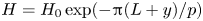 $H=H_0\exp ({-{\rm \pi} (L+ y)/p})$ with
  $H_0=422 \ \textrm {kA}\,\textrm {m}^{-1}$ and
  $p=0.118\ \textrm {m}$. The apparent mass density of the magnetic fluid with
 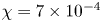 $\chi =7 \times 10^{-4}$ is indicated by the blue dashed line. The corresponding vertical axes are indicated by the arrows. The magnetic susceptibility is calculated by measuring the magnetization of the liquid using a vibrating sample magnetometer (EZ-9 from Microsense) and computing the slope of the
  $H$-
$H$- $M$ curve. During the measurement, the magnetic liquid showed no hysteresis, which indicates the paramagnetic behaviour of the liquid.
Table 1. Properties of the experimental set-up. The particles used for the experiments are spherical PVC-U ( ${p_1}$) and POM (
 ${p_2}$) beads. The paramagnetic liquid is a saturated aqueous solution of
  $\textrm {MnCl}_2$ salt. The molal concentration of the synthesized solution is
  $4.62\ \textrm {mol}\,\textrm {kg}^{-1}$. The susceptibility of the paramagnetic liquid is calculated by measuring the magnetization of the solution, and the dynamic viscosity of the liquid is measured using a rheometer.

5. Results and discussion
In this section, we first present and discuss our results for single- and two-particle systems. In these systems, the particle-induced flow is neglected, and the equations of motion of the fluid are not solved, which is valid at the very low particle volume fraction of these simulations. In § 5.3, we address many-particle systems in which we do solve the fluid equations and also consider two-way momentum coupling between the fluid and particles.
5.1. The motion of a single particle immersed in a quiescent paramagnetic liquid
The buoyancy-driven motion of spherical particles in Newtonian fluids has been extensively studied. It is shown experimentally (Horowitz & Williamson Reference Horowitz and Williamson2010) and numerically (Jenny et al. Reference Jenny, Dušek and Bouchet2004) that the motion of a freely falling or ascending sphere under the action of gravity in a Newtonian fluid is fully characterized by two dimensionless numbers, namely the particle relative mass density  $\rho _{p}/\rho _{f}$ and the Galileo number
  ${Ga}=\sqrt {|1-\rho _{p}/\rho _{f}|gd_{p}^{3} }/\nu$. For a particle settling in a magnetic liquid an ‘apparent Galileo number’ can be defined as
  ${Ga_a}= \sqrt {|1-\rho _{p}/\rho _{f,a}| gd_{p}^{3} }/\nu$. Unlike the settling of a particle in a non-magnetic liquid, for a particle travelling inside a magnetically responsive liquid in a direction parallel to the magnetic field gradient, the apparent Galileo number is not constant. This number is dependent on the local apparent mass density of the liquid and therefore on the position of the particle. The farther away the position of the particle from its equilibrium point, the larger will be the apparent Galileo number. As the particle approaches its equilibrium position, the apparent Galileo number goes to zero. For the magnetofluidic systems considered in this section, the range of the apparent Galileo number is
  $0 \leq {Ga_a} <150$. Within this range, it is known that, regardless of the particle mass density ratio, the particle trajectory is vertical and quasi-steady (Jenny et al. Reference Jenny, Dušek and Bouchet2004). Therefore, we can assume that the motion of a single particle in a quiescent magnetic fluid exposed to a magnetic field with negligible horizontal gradients is in the
  $y$-direction. Based on this assumption, the governing equation of motion of the particle can be reduced to a two-dimensional scalar nonlinear system. In the following section we will investigate the solution behaviour of such nonlinear systems.
5.1.1. Equilibrium position and nature of particle motion
In our analysis, we make the following simplifying assumptions. Considering the fact that the fluid is at rest  $(U_0 = 0)$, we neglect the effect of fluid motion on the particle. Based on our earlier discussion, considering the range of apparent Galileo number and the one-dimensional magnetic field, we can further assume that the particle does not undergo any rotational or lateral movement. Under these assumptions, (2.20) and (2.21) can be simplified to the following system of scalar equations:
 \begin{align} \left. \begin{gathered} \frac{\textrm{d}y}{\textrm{d}t}= v,\\ \frac{\textrm{d}v}{\textrm{d}t}= \frac{\rho_{p}}{\rho_{p}+0.5\rho_{f}} \left[ -\frac{\left( 1+0.15 R e_{{p}}^{0.687} \right)}{\tau_{{t},i}} v -\frac{3}{2} \left({\rm \pi} \rho_{f} \mu\right)^{1 / 2} d_{i}^{2}\int_{0}^{t} \frac{1}{(t-\tau)^{1 / 2}} \frac{\textrm{d}{v}}{\textrm{d}\tau}\,\textrm{d}\tau\right.\\ + \left. \left( \frac{\rho_{f,a}}{\rho_{p}}-1 \right) g \right]. \end{gathered} \right\} \end{align}
System (5.1) is a non-autonomous system of two first-order nonlinear differential equations. The time-dependency stems from the Basset history contribution. The equilibrium point of this system,  $\boldsymbol {Y}_e=(y_e,0)^T$, can be found by setting
  $({\textrm {d}y}/{\textrm {d}t},{\textrm {d}v}/{\textrm {d}t})^T=(0,0)^T$ and
  $t \rightarrow \infty$, where
  $y_e$ denotes the equilibrium position of the particle.
Given the initial position and velocity of the particle, a discretized form of system (5.1) can be solved to find the vertical position and velocity of the particle as functions of time. It is, however, useful to obtain a qualitative understanding of the behaviour of a particle near its equilibrium point, before solving the system. By neglecting the history force, we can approximate system (5.1) with the autonomous system
 \begin{equation} \left. \begin{gathered} \frac{\textrm{d}y}{\textrm{d}t}= v,\\ \frac{\textrm{d}v}{\textrm{d}t}= \frac{\rho_{p}}{\rho_{p}+0.5\rho_{f}} \left[ -\frac{\left( 1+0.15 R e_{{p}}^{0.687} \right)}{\tau_{{t},i}} v +\left(\frac{\rho_{f,a}}{\rho_{p}}-1 \right) g \right]. \end{gathered} \right\} \end{equation}
A dynamical analysis of the linearization of system (5.2) reveals that depending on the problem parameters, the nature of motion of particle in the vicinity of its equilibrium position is monotonic or oscillatory (for details of the dynamical analysis, the reader is referred to appendix A). Singh et al. (Reference Singh, Das and Das2018) followed a similar approach to investigate the motion of a water droplet in a saturated ferrofluid.
For a given magnetofluidic system, a critical particle diameter exists above which the particle behaviour changes from monotonic to oscillatory. The equilibrium point and the critical particle diameter for the onset of oscillatory behaviour near the equilibrium point are summarized in table 2 for the three possible magnet configurations.
Table 2. Particle equilibrium position and critical particle diameter for top-, bottom- and two-magnet configurations with magnetic fields following (2.7), (2.6) and (2.8), respectively.

To illustrate the dependency of particle dynamics on its diameter, we consider the bottom-magnet configuration presented in § 4 with parameters given in table 1. In this configuration, the equilibrium position of a particle with a mass density  $\rho _{{p}}=1.434 \times 10^{3} \ \textrm {kg}\,\textrm {m}^{-3}$ is
  $y_e=-0.35L$. The corresponding critical diameter is
 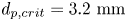 $d_{p,crit}=3.2 \ \textrm {mm}$. System (5.2) is solved by an explicit Euler method to obtain the vertical particle position as a function of time.
Figure 5 compares the time evolution of the vertical position of four particles with diameters of  $1$,
$1$,  $2$,
$2$,  $4$ and 6 mm obtained by solving system (5.2) with initial condition
 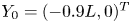 $Y_0=(-0.9L,0)^T$. The transition from monotonic to oscillatory motion can be observed by comparing the results of the 2 and 4 mm particles.The effect of particle size on the nature of particle motion can be further illustrated by the phase portraits and direction fields of system (5.2). Figure 6 compares the direction fields and phase portraits of solutions of this system obtained with combinations of three different initial positions, and three different initial velocities for (a)
  $d=2\ \textrm {mm}$ and
  $(\textit {b})\ d=6$ mm. Regardless of the initial condition, a 2 mm particle moves monotonically towards its equilibrium position, whereas a 6 mm particle exhibits a spiralling behaviour. Physically this difference can be easily understood: due to the larger magnetic buoyancy force, a 6 mm particle gains a larger velocity and overshoots the equilibrium point.

Figure 5. Effect of particle size on levitation dynamics. Time plots of vertical particle position for 1, 2, 4 and 6 mm particles.

Figure 6. Direction field and phase portraits for the solutions of system (5.2) with nine different initial conditions (black circles). The critical point of the system is 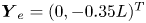 $\boldsymbol {Y}_e =(0,-0.35L)^T$ (red circle). The critical diameter for the considered parameters is
  $d_{p,crit }=3.2\ \textrm {mm}$. (a) Here
  $d_{p}=2\ \textrm {mm}$, the critical point is a node; (b)
  $d_{p}=6\ \textrm {mm}$, the critical point is a spiral point.
5.1.2. History effects
In the previous analysis, effects stemming from the Basset history force are neglected. However, it is known that the history force can be large at high particle acceleration rates. Therefore, in this section we investigate the effect of Basset history force on particle motion. Figure 7 compares the temporal evolution of position and velocity of a particle with  $d_{p}=2\ \textrm {mm}$ and
 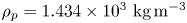 $\rho _{p} = 1.434 \times 10^3 \ \textrm {kg}\,\textrm {m}^{-3}$ with initial condition
 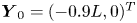 $\boldsymbol {Y}_0 =(-0.9L,0)^T$ over time interval
 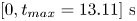 $[0,t_{max}=13.11]\ \textrm {s}$ with and without Basset history force. A window size of
 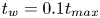 $t_w=0.1t_{max}$ is considered for the computation of the history kernel. For the
  $2$ mm particle, the history force leads to a slight decrease in the initial acceleration followed by a decrease in the deceleration of the particle as it approaches its equilibrium position. Initially the history force slows down the particle as it introduces extra damping to the system. As the particle gets closer to the equilibrium point the moving fluid drags the particle and reduces deceleration.
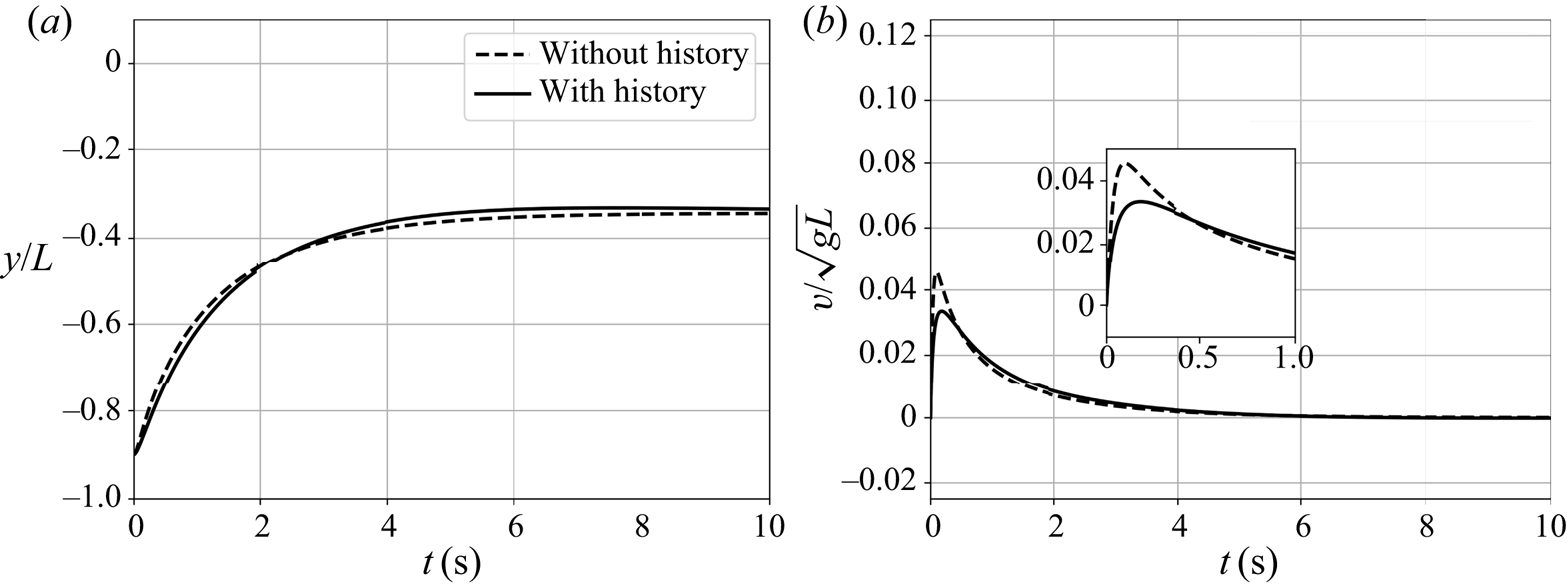


The effect of Basset history force on the motion of a larger particle is shown in figure 8 where the particle diameter is increased to  $6\ \textrm {mm}$. Although the history effects do not alter the oscillatory nature of the particle motion, it can be observed that the history force leads to an amplified overshoot near the equilibrium point. Physically, this can be interpreted as follows. As the particle approaches its equilibrium position, due to history effects, the moving fluid pushes the particle farther beyond the equilibrium point leading to a larger overshoot. However, the damping introduced by the history force decreases the particle oscillations.


The contribution of the Basset history force to the motion of a particle is further illustrated in figure 9, where different hydrodynamic forces acting on the particle are compared for  $d_{p}= 2$ and
  $6\ \textrm {mm}$. Note that the forces are normalized by the gravitational force. We observe that for both particle sizes, the added mass force has the smallest relative contribution to the particle motion. For the larger particle, the maximum absolute values for normalized steady drag and Basset history forces are smaller and are attained later. This explains the higher acceleration of the 6 mm particle. Thanks to particle's higher inertia, for the 6 mm particle the relative contribution of the Basset history force is larger compared with the steady drag force. Moreover, for a larger particle, the history force has an appreciable contribution over a larger fraction of the levitation time.

Figure 9. Temporal evolution of the added mass, static drag, Basset history and buoyancy force normalized by the gravitational force during the motion of a spherical particle with (a)  $d_{p}= 2\ \textrm {mm}$ and (b)
  $d_{p}= 6\ \textrm {mm}$.
5.2. Experimental validation of the mathematical model
In this section, we compare the solutions of systems (5.1) and (5.2) with experimental observations. First, we test our mathematical model against single-particle levitation experiments. Next, we consider two-particle systems where the effect of collisions is investigated.
5.2.1. Single-particle systems
For the single-particle measurements, we consider two spherical PVC-U particles with diameters  $d_{p}=3$ and
  $d_{p}=5\ \textrm {mm}$, and mass density
  $\rho _{p,1}$. The other problem parameters are identical to those given in table 1. It was shown numerically in § 5.1.2 that neglecting the history effects introduces an error which increases at larger particle sizes. In order to validate this, we compare the experimental recordings of vertical particle position with the results of the numerical simulations obtained with the same initial conditions.
For each particle, two sets of experiments are performed, a sinking and a rising experiment. The equilibrium height of the considered PVC-U particles is  $y_e=-0.35L$. For the sinking case, the particle is released at the top, and for the rising case, the particle is released at the bottom of the tank. Figure 10 compares the numerical solution of system (5.1) which includes the Basset history force, to that of the reduced system (5.2), and the experimental vertical position of the particles. Each experiment is repeated six times, and the results are averaged. The error bars correspond to the standard deviation of these six measurements. The considered history window size for the simulations is
  $t_{win}=0.2\ \textrm {s}$. The larger error bars in the experimental results of the 3 mm particle are due to the fact that the slower motion of smaller particles is relatively more sensitive to small disturbances in the flow. A very good agreement is observed between the numerical results with Basset history force and the experimental recordings. The larger contribution of history force to particle motion at larger diameters can be observed by comparing the plots of the 3 and 5 mm particles. It can clearly be seen from figure 10(c) that exclusion of Basset history force leads to a
  $35\,\%$ underestimation of the settling time for the falling 5 mm particle (
 $6.22\ \textrm {s}$ versus
  $4.00\ \textrm {s}$). For the rising 5 mm particle (figure 10d) an underestimation as high as
  $47\,\%$ is observed (
 $4.98\ \textrm {s}$ versus
  $2.65\ \textrm {s}$). These observations prove that system (5.1) describes the vertical motion of a single spherical particle very well, and that the contribution of Basset history force is crucial for accurate prediction of the motion of single particles of larger diameters in a paramagnetic liquid. The numerical results presented in the rest of the paper are obtained by the numerical model which includes the Basset history force, unless stated otherwise.

Figure 10. Vertical position of  $3$ and
  $5$ mm PVC-U particles. The dashed curves corresponds to numerical solutions of system (5.1). The dotted lines indicates the particle position obtained from solving reduced system (5.2) and the solid curve corresponds to the experiments. (a) Falling 3 mm particle. (b) Rising 3 mm particle. (c) Falling 5 mm particle. (d) Rising 5 mm particle.
5.2.2. Effect of collisions: two-particle systems
In a many-particle MDS system, a particle can undergo multiple collisions as it moves towards its equilibrium position. Collisions are expected to hamper the motion of the particle and therefore delay the separation. In this section, we first present the experimental procedure for obtaining the effective coefficients of friction and tangential restitution. Next, we test our hard-sphere model by comparing the results of numerical simulations with experimental observations on two colliding particles.
Experimentally, collisions are obtained by releasing two properly selected particles simultaneously from the top and bottom of the tank. The considered particles for the experiments are a 5 mm PVC-U particle with mass density  $\rho _{p,1}$ (the sinking particle), and a 5 mm POM particle with mass density
  $\rho _{p,2}$ (the rising particle). Depending on the offset between the centre of the particles, the lateral centre distance (
 $LCD$), collisions can range from ‘head-on’ to ‘grazing’. We define an impact factor as
 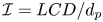 $\mathcal {I} = {{LCD}}/{d_{p}}$, where for
  $\mathcal {I}=0$ a collision is head-on and
  $\mathcal {I}=1$ corresponds to a grazing collision.
Yang & Hunt (Reference Yang and Hunt2006) found that lubricated contact during collisions with low binary Stokes numbers reduces the dependence of rebound motion on the tangential particle–particle interactions. The dominating hydrodynamic effects of the interstitial fluid on the tangential component of motion during a collision can be captured by incorporating an effective (lubricated) friction coefficient. The two remaining effective collision parameters are obtained by investigating the tangents of incident and rebound at various particle–particle collisions. The binary normal Stokes number for the considered collisions are in the range  $0 < {St_{n}} \leq 14$. Considering the zero precollision angular velocity and the small particle rotational relaxation time, the angular velocities remain almost zero after the collision. The tangent of rebound is therefore purely based on the translational particle velocity. In figure 11 the tangent of rebound angle for
  $40$ different collisions is plotted against the tangent of incident angle. The positivity of
  $\psi _{out}$ indicates the absence of the sticking regime. This reduces the number of required collision parameters to two, as the tangential restitution coefficient is only needed for capturing sticking collisions. The lubricated friction coefficient,
  $\mu _{eff}$, is found by fitting the line
  $\psi _{out}=\psi _{in}- ({7}/{2})(1+e_{n,{eff}})\mu _{eff}$ to the data, where
  $e_{n,{eff}}$ is calculated by (2.33) with
  $e_{n,{dry}}=0.86$ and
  $\eta _e=1.5\ \mathrm {\mu }\textrm {m}$. Depending on the value of
  $e_{n,{eff}}$, the lubricated friction coefficient ranges from
 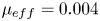 $\mu _{eff}=0.004$ to
 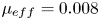 $\mu _{eff}=0.008$. We use an average value of
  $\mu _{eff}=0.005$ in our collision model.

Figure 11. The tangent of rebound angle as a function of the tangent of incident angle for a 5 mm PVC-U particle colliding with a 5 mm POM particle. Each point represents one collision experiment.
Figure 12 compares the vertical position of the particles versus time, obtained from numerical simulations and experimental recordings for three collisions, with impact factors  $\mathcal {I}=0.02$,
  $\mathcal {I}=0.41$ and
  $\mathcal {I}=0.78$. The numerical results are performed with a one-way coupled model using the same initial positions and velocities as in the experiments. To facilitate the comparison, the numerical results are slightly shifted in time to match the numerically and experimentally obtained collision times. A remarkably good agreement is observed between the numerically and experimentally obtained vertical positions of the particles as functions of time. The maximum increase in the levitation time is caused by the collision with
  $\mathcal {I}=0.02$. This collision leads to approximately
  $15\,\%$ and
  $45\,\%$ increases in the levitation time of the sinking and rising particle, respectively (based on experiments).

Figure 12. Temporal evolutions of vertical positions of particles during binary collisions between a rising PVC-U particle and a falling POM particle with three different impact factors: (a)  $\mathcal {I}=0.02$; (b)
  $\mathcal {I}=0.41$; (c)
  $\mathcal {I}=0.78$. The size of the particles are indicated by the vertical bars. Movies of the binary collision experiments and simulations are found as supplementary movies 1, 2 and 3 available at https://doi.org/10.1017/jfm.2020.1001.
The horizontal motion of the particles can be seen in supplementary movies 1, 2 and 3. In contrast to the vertical direction, some discrepancies are observed between the numerically and experimentally obtained results. These discrepancies are due to the magnetic field non-uniformities in off-centre regions of the experimental set-up. The gradient of the magnetic field strength is vertical only in the central region of the tank. Hence, the assumption of vertical magnetic buoyancy force is only valid in this central region. Once particles undergo a collision, they enter regions where the magnetic buoyancy force is not vertical. In these regions, the horizontal gradient in the magnetic field strength pushes the particles back to the centre of the tank. This results in deviations from the numerically obtained post-collision horizontal motion of the particles.
5.3. Many-particle systems
In § 5.2, we validated our numerical model by comparison with experimental measurements of single- and two-particle systems. In this section, we present the results of the application of this numerical model to many-particle systems. We assume a uniform initial flow field with no disturbances. Particle-induced flow disturbances are taken into account by considering two-way momentum transfer between the fluid and the discrete spherical particles as described in § 3.3. A two-magnet configuration is considered where levitation of particles both lighter and heavier than the carrier liquid is possible. The magnetic field is described by (2.8). The computational domain has dimensions  $L_x=4 {\rm \pi}L/3$,
  $L_y= 2L$ and
  $L_z= 4 {\rm \pi}L/3$, as depicted in figure 13. The particle volume fraction is kept constant at
  $\phi =0.02$ which is a relevant value in practical MDS applications (Bakker et al. Reference Bakker, Rem and Fraunholcz2009). Moreover, one should note that the applicability of the numerical model presented in this work is limited to low particle volume fractions, i.e.
  $\phi < 0.05$. The physical properties of the many-particle configurations are summarized in table 3.

Figure 13. A schematic of the computational domain for the many-particle simulations. In a frame moving with the same velocity as the conveyor belts,  $U_0 \boldsymbol {i}$, the mean streamwise velocity of the fully developed flow is zero. In this frame, the walls at
  $y=\pm L$ are at rest.
Table 3. Parameters used for the many-particle simulations.

As mentioned in § 1, in most recent MDS systems conveyor belts are installed at the top and bottom of the channel. These conveyor belts move with the same speed as the mean streamwise velocity  $U_0$. This circumvents the formation of boundary layers and transition to turbulence near the walls. For such flow configurations, it is convenient to solve the governing equations in a frame moving in the
  $x$-direction with the mean streamwise flow velocity
  $U_0$. In this frame, the mean velocity of the fully developed flow is zero, and the top and bottom walls are at rest. Therefore we impose no-slip and no-penetration velocity boundary conditions at
  $y/L=\pm 1$, where the surfaces of the two magnets are located. In the
  $x$- and
  $z$-directions periodic boundary conditions are imposed.
Figure 14(a) shows the magnitude of the magnetic field, and the corresponding effective mass density of the magnetic fluid as functions of  $y$. According to (2.17) and (2.19), this configuration is capable of sorting a mixture
 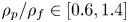 $\rho _{p}/\rho _{f} \in [0.6,1.4]$ (
 $|\Delta \rho _{f,a}|_{max} =0.4\rho _{f}$), with
 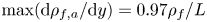 $\max ({\textrm {d}\rho _{f,a}}/{\textrm {d}y})=0.97\rho _{f}/L$ at the surface of the magnets. Particles with mass densities in the range of
  $\rho _{p,k}/\rho _{f}\in [0.7,1.3]$ are uniformly distributed over 10 mass density groups. These mass densities and their corresponding equilibrium heights are indicated by dashed lines in figure 14(a). Particles are initially randomly distributed in two injection zones at the bottom, (
 $-1<y/L<-0.75$) and top (
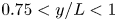 $0.75<y/L<1$) of the channel. The injected particles are preseparated into two groups of light and heavy particles. Particles heavier than the carrier liquid (
 $\rho _{p,h} /\rho _{f} \in (1,1.3]$) are injected at the bottom, and particles lighter than the liquid (
 $\rho _{p,l} /\rho _{f} \in [0.7,1]$) are injected at the top of the domain. For a more realistic initial condition, a particle impurity is considered in each injection zone. The particle impurity is defined as
  $\textrm {Imp}={N_{p,h}}/{N_{p,top}}={N_{p,l}}/{N_{p,bottom}}$, where
  $N_{p,top}$ and
  $N_{p,bottom}$ are the total numbers of particles injected in the top and bottom injection zones. Here
  $N_{p,l}$ and
  $N_{p,h}$ are the number of light and heavy particles, respectively. In case of a perfect preseparation,
  $\textrm {Imp}=0$, whereas
  $\textrm {Imp}=0.5$ indicates no preseparation (fully random particle distribution). For particles that are not preseparated, during a short time interval, the apparent Galileo number can be in the range
  $Ga \in [150,218]$. We ignore deviations from the steady vertical motion, caused by the transition in the wake of these particles.

Figure 14. (a) Magnetic field strength profile and the corresponding profile of the effective mass density of the magnetic fluid. The dotted lines indicate mass densities of the particles. The dashed lines correspond to the considered cut mass densities. The corresponding vertical axes are indicated by the horizontal arrows. (b) Critical particle diameter as a function of mass density.
The critical particle diameter as a function of particle mass density derived in § 5.1.1, is plotted in figure 14(b). The maximum critical particle diameter corresponding to neutrally buoyant particles ( $\rho _{p}/\rho _{f}=1$) is approximately
  $5.3\ \textrm {mm}$. It is noteworthy that although the magnetic configuration is fully symmetric, the critical particle diameter profile is asymmetric: particles lighter than the magnetic liquid have a larger critical diameter than heavier particles with the same mass density difference.
The time step size is  $0.0009\ \textrm {s}$. The numbers of Fourier modes in streamwise and spanwise directions are
  $256$, and the wall-normal direction consists of
  $129$ grid points. A window size of
  $0.01 t_{max}$, with
  $t_{max}=35\ \textrm {s}$, is considered for the calculation of the Basset history force. The initial particle–fluid relative velocity is assumed to be zero. Interparticle and wall–particle collisions are treated by the hard-sphere model addressed in § 2.4.2. Based on the results of § 5.2.2, we consider an average value of
  $0.85$ for the dry coefficient of normal restitution. The average lubricated friction coefficient is assumed to be
  $0.005$.
In order to investigate the effect of different parameters on the separation performance, we study six different test cases. Case 1A is considered as the base case. We study the effects of neglecting history force, two-way coupling and particle–particle interactions on the collective motion of particles in cases 1B, 1C and 1D, respectively. In case 2, the effect of the particle size is studied by decreasing the particle size from  $4$ to
  $2\ \textrm {mm}$. Finally, case 3 addresses the effect of particle preseparation. The parameters of the test cases are summarized in table 4.
Table 4. Summary of test cases.

We quantify the separation performance by the root mean square of the distances of the particles from their theoretical equilibrium point given in table 2. We define the non-dimensional separation error as
 \begin{equation} e_{m}(t)=\frac{1}{L}\sqrt{\frac{1}{N_{p}}\sum_{i=1}^{N_{p}}(y_{{p},i}(t)-y_{e,i})^2}, \end{equation}
where  ${N_{p}}$ is the number of particles,
  $y_{{p},i}(t)$ is the position of a particle at time
  $t$ and
  $y_{e,i}$ denotes its equilibrium height. The mean separation error defined by (5.3) can be evaluated for all particles to assess the overall temporal performance of the system, but also for each individual mass density group. In the former,
  $N_{p}$ is the total number of particles, whereas for the latter
  $N_{p}$ is the number of particles in the mass density group.
5.3.1. Case 1: effects of history force, collisions and two-way coupling
Figure 15 shows a cross-section of the velocity field and front view of the particle distribution in the moving frame at  $t=0.01\ \textrm {s}$,
  $t=0.5\ \textrm {s}$,
  $t=1.0\ \textrm {s}$,
  $t=1.5$,
  $t=2\ \textrm {s}$ and
  $t=2.5\ \textrm {s}$ for case 1A where history effects, two-way coupling and collisions are taken into account. The horizontal colour bar shows the wall-normal component of the particle-induced fluid velocity, and the vertical colour bar corresponds to the particle mass density ratio
  $\rho _{p}/\rho _{f}$. It can be seen that after
  $2.5\ \textrm {s}$, all particles have almost reached their equilibrium positions. A higher level of particle dispersion is observed in the central region of the channel than in the vicinity of the walls. First, particles with equilibrium positions in the central region interact more with other particles as they move to their equilibrium height. Second, the lower magnetic field gradient in the central region leads to a slower vertical motion of these particles and therefore a longer separation time.

Figure 15. Cross-sections of the velocity field in the moving frame at the plane where  $z={L_z}/{2}$, and projections of the particles in the section of the domain where
  $|z-{L_z}/{2}|< 3d_{p}$ (case 1A). The particles are coloured based on their relative mass density
  $\rho _{p}/\rho _{f}$ (vertical colour bar). The horizontal colour bar corresponds to the streamwise component of the particle-induced fluid velocity. A movie corresponding to this figure (supplementary movie 4), and a three-dimensional animation of the particle separation (supplementary movie 5) are found in the supplementary material.
The effects of history force, two-way coupling and collisions on the system overall separation performance are illustrated in figure 16(a) where the mean separation errors for cases 1A–1D are plotted as functions of time. When history, two-way coupling and collision effects are taken into account the time required to obtain a mean separation error of  $0.02$ is approximately
  $3\ \textrm {s}$. This effectively means that achieving this separation accuracy at a mean streamwise velocity
  $U_0$ requires the length of the separation channel to be at least
  $3U_0$.

Figure 16. (a) Average separation error versus time for cases 1A, 1B, 1C and 1D. (b) Average separation error per mass density as a function of time for case 1A.
The decay behaviour of the mean separation error is almost identical for cases 1A–1D until  $t=1\ \textrm {s}$. After this time, the decay rates for the cases without history force and collisions begin to deviate. Two-way coupling appears to have a negligible effect on the overall separation performance. Collisions increase the time required to achieve an average separation error of
  $0.02$ by approximately
  $0.5\ \textrm {s}$. The effect of the history force is more drastic. Neglecting the history force leads to an underestimation of approximately
  $1.5\ \textrm {s}$ in achieving
  $e_{m} =0.02$. When history effects are neglected, the average separation error decreases monotonically, whereas, with history force included, the mean separation error reaches a plateau at
  $t \approx 1.5\ \textrm {s}$. History effects introduce additional resistance to particle levitation. Moreover, when a particle reaches its equilibrium point, the history force drags the particle away from it. Both effects lead to a decrease in the decay rate of the average separation error of the system.
Temporal evolutions of average separation errors per mass density group for case 1A are compared in figure 16(b). Until  $t\approx 1\ \textrm {s}$, all mass density groups show a similar decay behaviour. At a given time
  $t > 1.3\ \textrm {s}$, the larger the absolute fluid–particle mass density difference of a group, the smaller is the average separation error of that group. The distinguishing behaviour of mass density groups with
  $|1-\rho _{p}/\rho _{f}|=0.03$ is interesting. On average, particles in these mass density groups travel the longest distance to reach their equilibrium positions. Owing to history effects, these particles overshoot their equilibrium positions. Moreover, compared with other particles, the ‘restoring’ magnetic buoyancy force acting on particles in these groups is smaller in the central region of the channel where the gradient of the magnetic field is low. These two effects lead to a period of increase in the separation error between
  $t\approx 1.3\ \textrm {s}$ and
  $t \approx 1.7\ \textrm {s}$. A similar behaviour is observed for groups with
  $|1-\rho _{p}/\rho _{f}|=0.3$ and
  $|1-\rho _{p}/\rho _{f}|=0.23$ during the interval
  $t\in [1.25,2]$ when the particles which were in the ‘wrong’ injection zone reach their equilibrium positions.
To illustrate the effect of collisions and history force on the temporal evolution of the local distribution of particles, in figure 17 the probability density function of the vertical position of particles for cases 1A, 1B and 1C are compared. After only  $0.96\ \textrm {s}$, a clear difference is observed in the distributions of the particles when history effects are neglected. The history force enhances particle dispersion and causes a larger variance in particle positions. The effect of history force becomes more prominent at
  $t=2\ \textrm {s}$. Without history effects, the distribution of particle positions in the central region deviates both in variance and average value. Collisions, on the other hand, only influence the variance of the particle position. The effect of collisions is stronger for particles with equilibrium positions in the central region, since these particles travel over a larger vertical distance and collide more often.The results presented in the following subsections include the history force, collisions and two-way coupling.

Figure 17. Evolution of probability density function of particle position for cases 1A, 1C and 1D. The corresponding animation, supplementary movie 6 is available in the supplementary material. The movie on the right corresponds to the case 1A (the base case).
5.3.2. Cases 2 and 3: effects of particle size and preseparation
We investigate the effect of particle size on the separation performance by changing the particle size from  $4\ \textrm {mm}$ to
  $2\ \textrm {mm}$ while the total volume fraction of particles is kept constant. Figure 18 compares the temporal evolution of average separation errors for the two considered particle sizes. The average separation error for 2 mm particles after
  $5$ seconds is
  $0.3$ while this value for 4 mm particles is as low as
  $0.01$. The superior separation performance of case 1A is in line with the findings of § 5.1.1. The difference between the decay behaviour stems from the higher magnetic force on the larger particles. Moreover, with a constant volume fraction, smaller particles collide more frequently with other particles which leads to a lower separation performance. As can be seen in figure 14,
  $d_{p}=2\ \textrm {mm}$ is smaller than the smallest critical particle diameter. Therefore, a
  $2$ mm particle exhibits a non-oscillatory motion towards its equilibrium point, leading to a monotonic decay of the average separation error.

Figure 18. The effect of particle size and preseparation on the mean separation error.
The dash-dotted line in figure 18 shows the temporal evolution of the mean separation error for an initial impurity of  $0.5$. This corresponds to a case where particles are not initially separated into two mass density groups of heavy and light particles but are randomly distributed over both injection regions. This has a negative effect on the separation performance since particles have to travel farther to reach their equilibrium position, which also results in a larger number of collisions. Preseparation decreases the time required to obtain an average separation error of
  $0.02$ by approximately
  $33\,\%$ (
 $3\ \textrm {s}$ versus
  $4\ \textrm {s}$).
6. Conclusions and outlook
In this work, we presented a point-particle Euler–Lagrange approach which can accurately capture the collective motion of almost neutrally buoyant particles in the flow of magnetically responsive liquids. Numerical simulations are performed on single and multiparticle systems over the range of apparent Galileo number  $0 \leq Ga_a < 220$. This has relevant applications in MDS systems, which are used for the separation of different types of plastic. The numerical results of single- and two-particle simulations are in good agreement with detailed experimental results on particle position.
It is shown that when history force is neglected, a maximum of five parameters can characterize the buoyancy-driven vertical motion of a spherical particle towards its equilibrium point. We compared the contributions of different hydrodynamic forces to the motion of a single particle and showed that the Basset history force is important for large particles. It is found that neglecting history force at large particle diameters can lead to a significant underestimation of the levitation time.
We presented a hard-sphere collision modelling strategy which can accurately capture interparticle interactions in a magnetized paramagnetic liquid. Numerical and experimental investigations of binary collisions considered in this study show that depending on the impact factor a single particle–particle collision can lead to up to approximately  $45\,\%$ increase in the particle levitation time. The separation performance of large MDS systems where up to approximately
  $18\,000$ particles are levitated is quantified by evaluating the mean separation error. Particularly, the effects of particle size and particle preseparation have been studied. The investigations revealed that the effects of history force and collisions are important even at particle volume fractions as low as
  $2\,\%$. Neglecting history force and collisions lead to an erroneously reduced particle dispersion, especially for particles with mass density ratio close to one. Our numerical results showed that an increase in the particle size from
  $4$ to
  $2\ \textrm {mm}$ increases the time required to achieve an average separation error of
  $0.02$ by around
  $40\,\%$, indicating the importance of particle size distribution in MDS applications. The method described in this paper is a firm basis for the development of useful design rules for optimization of future magnetic separation technologies.
As a natural starting point for most studies on particle-laden flows, this work was based on the assumption of spherical particle shape. However, it is well known that particle non-sphericity has a significant influence on fluid–particle interactions, and therefore on the dynamics of particles. Furthermore, this work did not consider the effect of background flow disturbances on the motion of particles. Background turbulence can remarkably delay the levitation time as particles in MDS typically have mass density ratios close to one. Such particles have small relaxation times, and their motion is therefore sensitive to a background flow. These two aspects are open to future research.
Supplementary movies
Supplementary movies are available at https://doi.org/10.1017/jfm.2020.1001.
Acknowledgements
The authors acknowledge J.R. Wubs for her work on the characterization of the magnetic liquid and the magnetic field. We thank A.M. van Silfhout for measuring the magnetic susceptibility of the liquid. We are grateful to our technicians G.W.J.M. Oerlemans, J.M. van der Veen and A.P.C. Holten for their help in the design and construction of the experimental set-up. We also thank B. Hu and J. Wijnja from Umincorp for insightful discussions.
Funding
This work is part of the research programme ‘Innovative Magnetic Density Separation for the optimal use of resources and energy’ under project number 14916, which is partly financed by the Netherlands Organisation for Scientific Research (NWO). This work was sponsored by NWO Exact and Natural Sciences for the use of supercomputer facilities.
Declaration of interests
The authors report no conflict of interest.
Appendix A. Dynamical analysis of single-particle motion
In this Appendix we present a dynamical analysis through which the solution behaviour of system (5.1) is characterized. For brevity we present our analysis for a bottom-magnet configuration where the fluid apparent mass density follows (2.6).
System (5.1) can be written in matrix notation as
 \begin{equation} \dot{\boldsymbol{Y}}=\frac{\textrm{d} \boldsymbol{Y}}{\textrm{d}t}=\boldsymbol{F}(\boldsymbol{Y},t),\end{equation}
where
 \begin{align} \boldsymbol{Y}={\begin{pmatrix} {y} \\ v\end{pmatrix}} \end{align}
and
 \begin{equation} \boldsymbol{F}(\boldsymbol{Y},t)={\begin{pmatrix} {v} \\ \alpha \xi v+ \eta\xi +\beta\xi \textrm{e}^{\theta y}+\alpha \epsilon\xi v|v|^{0.687}+\zeta \xi \displaystyle\int_{0}^{t} \dfrac{1}{(t-\tau)^{1 / 2}} \dfrac{\textrm{d}{v}}{\textrm{d}\tau}\,\textrm{d}\tau \end{pmatrix}} \end{equation}
with
 \begin{equation} \left. \begin{gathered} \alpha = - \frac{1}{\tau_\textrm{t}}, \quad \eta =\left(\frac{\rho_{f}}{\rho_{p}}-1\right)g,\quad \beta= \frac{2{\rm \pi} \mu_0 \chi H_0^2 }{pg\rho_{p}}\textrm{e}^{-2{\rm \pi} L/p},\quad \theta=-\frac{2{\rm \pi}}{p},\\ \epsilon=-0.15 \left(\frac{d_{p}}{\nu}\right)^{0.687}, \quad \zeta=-1.5\left({\rm \pi} \rho_{f} \mu\right)^{1 / 2} d_{p}^{2}, \quad \xi=\frac{\rho_{p}}{\rho_{p}+0.5\rho_{f}}. \end{gathered} \right\} \end{equation}
By setting  $\dot {\boldsymbol {Y}}=(0,0)^T$ and
  $t \rightarrow \infty$, the history integral term tends to zero as
  $t \rightarrow \infty$ and the equilibrium point of the system reads
 \begin{equation} \boldsymbol{Y}_e= \begin{pmatrix} y_e\\ {0} \end{pmatrix} = \begin{pmatrix} \dfrac{1}{\theta}\ln \left(\dfrac{-\eta}{\beta}\right)\\ {0} \end{pmatrix},\end{equation}
where  $y_e$ corresponds to the equilibrium position of the particle in the magnetic liquid. Considering the fact that
  $\beta >0$, an equilibrium point exists only if
  $\eta <0$, i.e.
  ${\rho _{f}}/{\rho _{p}}\leq 1$. This implies that a bottom-magnet configuration is only capable of levitating particles which are heavier than the magnetic liquid. Particles which are lighter will eventually float on top of the liquid.
If we now assume that the history force is negligible compared with the other forces acting on the particle, system (A1) can be converted to an autonomous system of the form
 \begin{equation} \dot{\boldsymbol{Y}}=\frac{\textrm{d}\boldsymbol{Y}}{\textrm{d}t}=\boldsymbol{G}(\boldsymbol{Y}), \end{equation}
where
 \begin{equation} \boldsymbol{G}(\boldsymbol{Y})=\begin{pmatrix} {v} \\ \alpha \xi v+ \eta\xi +\beta\xi\textrm{e}^{\theta y}+\alpha \epsilon\xi v|v|^{0.687} \end{pmatrix}. \end{equation}
 Without loss of generality we can shift the equilibrium point of the system to the origin by making the substitution  $\tilde {\boldsymbol {Y}}=\boldsymbol {Y}-\boldsymbol {Y}_e$. Near the equilibrium point,
  $\tilde {\boldsymbol {Y}} \rightarrow (0,0)^T$. Therefore, system (A7) can be approximated by the linear system
 \begin{equation} \dot{\tilde{\boldsymbol{Y}}}={\boldsymbol{\mathsf{J}}}\tilde{\boldsymbol{Y}}, \end{equation}
where the Jacobian matrix  ${\boldsymbol{\mathsf{J}}}$ is
 \begin{equation} {\boldsymbol{\mathsf{J}}}= \begin{pmatrix} 0 & 1 \\ \beta \theta \xi \textrm{e}^{\theta y_e} & \alpha \xi \end{pmatrix}= \begin{pmatrix} 0 & 1 \\ -\eta \theta \xi & \alpha \xi \end{pmatrix}. \end{equation}
The stability and type of the critical point of the system (A8) are determined by eigenvalues of the matrix  ${\boldsymbol{\mathsf{J}}}$,
  $\lambda _{1,2}=\alpha \xi /2 \pm (\alpha ^2 \xi ^2/4 - \eta \theta \xi )^{0.5}.$ It can be shown that except for the special case where
  $\alpha ^2/4 = \eta \theta$, the stability and type of the critical point are not affected by the nonlinear terms in the system (A6). Therefore the behaviour of the solution of nonlinear system (A6) can be determined by studying the much simpler linear system (A8). In the case of an existing equilibrium point, considering the fact that
  $\alpha \xi <0$ and
  $\eta \theta \xi >0$, the eigenvalues are either negative real numbers or complex numbers with a negative real part. Therefore the solution of the system is always asymptotically stable. The behaviour of the solutions is dependent on the sign of
  $(\alpha ^2 \xi ^2/4 - \eta \theta \xi )$. If
  $\alpha \xi /2 >\sqrt {\eta \theta \xi }$, the eigenvalues are real and the equilibrium point is an asymptotically stable node. The particle, in this case, monotonically moves towards its equilibrium point. On the other hand, for
  $\alpha \xi /2< \sqrt {\eta \theta \xi }$ the eigenvalues are complex numbers. The equilibrium point, in this case, is a spiral point; the particle exhibits an oscillatory motion around the equilibrium point while it approaches it. For a fixed magnetofluidic configuration a critical particle diameter can be found above which oscillatory behaviour occurs. This critical diameter for a single-magnet configuration, regardless of the magnet position is
 \begin{equation} d_{p,crit }=\left[\frac{81 \mu^{2} p}{ {\rm \pi}\left(\rho_{{p}}-\rho_{{f}}\right)\left(2\rho_{{p}}+\rho_{{f}}\right) g}\right]^{0.25}. \end{equation}
A similar analysis can be performed for top-magnet and two-magnet configurations with magnetic fields described by (2.7) and (2.8), respectively. The results are summarized in table 2. It is notable that for one-magnet configurations the particle behaviour is dependent on four parameters only, namely  $\alpha$,
  $\eta$,
  $\theta$ and
  $\xi$. For two-magnet systems the nature of particle motion is also dependent on the parameter
  $\beta$.


 Open access