2.1. Turbulent closure for the linearised momentum equations

We take up the work by Charru et al. (Reference Charru, Andreotti and Claudin2013) to solve the linearised momentum equations, considering a steady and incompressible fluid flow, the corrugated surface being fixed in time at this stage. The notation and the system of equations are recalled in Appendix A.1. The study is restricted to the linear response of the flow to the wall undulation, i.e. the amplitude $\zeta _0$ of the wall deformation is small enough compared with the wavelength ${2{\rm \pi} }/{\alpha }$, with $\alpha$ the wavenumber. The nonlinear limit is $\alpha \zeta _0 \approx 0.1$ (Charru et al. Reference Charru, Andreotti and Claudin2013) whereas flow separations are expected for $\alpha \zeta _0>0.3$ (Zilker & Hanratty Reference Zilker and Hanratty1979). A dedicated code based on a collocation method (Canuto et al. Reference Canuto, Hussaini, Quarteroni and Zang2006) using Chebyshev polynomials was developed to solve the linearised system. The Reynolds stresses are modelled with the help of the Boussinesq hypothesis (A3) and the eddy viscosity $\nu _t$ is deduced from a mixing length approach (A2). Thorsness et al. (Reference Thorsness, Morrisroe and Hanratty1978) first proved that a correction is required to recover the experimental results (Zilker et al. Reference Zilker, Cook and Hanratty1977) showing large phase shifts of the wall shear stress with respect to the wall undulation in a specific wavenumber range, as illustrated in figure 2. The idea is to introduce a dependence to a relaxed pressure gradient for the van Driest number $A$ inspired by the work of Loyd, Moffat & Kays (Reference Loyd, Moffat and Kays1970) or similarly by that of Cebeci & Smith (Reference Cebeci and Smith1974). Since the mixing length $l$ (A2) depends on the non-dimensional variables, the wall normal coordinate $\eta$, the Reynolds number $\mathcal {R}$ based on the wavenumber $\alpha$ and the van Driest number $A$, the disturbed part of the mixing length $\hat {l}$ obtained after linearisation contains three distinct contributions

(2.1)\begin{equation} \hat{l} =-\kappa\left[1-\exp\left(-\frac{\mathcal{R}\eta}{A^0}\right) \left(1-\frac{\mathcal{R}\eta}{A^0}+\frac{\mathcal{R}\eta^2}{A^0} \left(\frac{\hat{\tau}_{xz}}{2}-\beta\mathcal{C}\right)\right)\right]. \end{equation}

The first one due to $\eta$ is the linearised effect of the geometrical deformation. The second reveals the influence of the wall shear stress disturbance $\hat {\tau }_{xz}$. Finally, the dependence to $\mathcal {C}$ is brought by the van Driest constant $A$ with $\beta$ the relative variation of $A$ due to the relaxed pressure gradient $\beta =({1}/{A^0})({\partial {A}}/{\partial {\mathcal {C}}})$. The parameter $A^0=26$ is the standard van Driest constant and $\beta =35$ is found to be the value that best fits the measurements (Frederick & Hanratty Reference Frederick and Hanratty1988; Charru et al. Reference Charru, Andreotti and Claudin2013). The dimensionless correction $\mathcal {C}$ is given by a differential equation that reads

(2.2)\begin{equation} \gamma \frac{\partial{\mathcal{C}}}{\partial{x}}=\frac{1}{u_{\tau}^2}\frac{\partial{}}{\partial{x}} \left(\tau_{xx}-\frac{p}{\rho}\right)-\mathcal{C} ,\end{equation}

where $p$ is the pressure, $\rho $ the density and $u_{\tau}$ the friction velocity. The constant $\gamma$ determines the length over which the relaxation operates with respect to the streamwise gradient of $\tau _{xx}-{p}/{\rho }$. Originally (Thorsness et al. Reference Thorsness, Morrisroe and Hanratty1978; Frederick & Hanratty Reference Frederick and Hanratty1988), $\mathcal {C}$ was only related to the pressure gradient, with similar results. The dimensionless quantity $\mathcal {C}$ does not correspond to the whole correction introduced in $\hat {l}$, but it will be called Hanratty's correction thereafter for brevity. When only the geometrical dependence of $\hat {l}$ is kept, and so the dependences on $\hat {\tau }_{xz}$ and $\mathcal {C}$ are dropped in (2.1), the turbulence can be seen as ‘frozen’ regarding the perturbations. This will be referred to as the frozen turbulence assumption in the following. More details on (2.1) and (2.2) can be found in the supplemental material of the review of Charru et al. (Reference Charru, Andreotti and Claudin2013).

Figure 2. Phase of the wall shear stress in the transitional regime. Filled black circles denote Hanratty's experimental results. Solid lines are results of the linear analyses with the Hanratty correction $\mathcal {C}$ (blue) and under the frozen turbulence hypothesis (orange). Rectangles are results of RANS computations with the $k\unicode{x2013}\omega$ model (orange) and the elliptic blending Reynolds stress model (blue). Forced responses in channel flow are plotted with dashed blue lines for $\alpha \delta =2{\rm \pi}$ and $\beta =40$: – – –; $\alpha \delta ={\rm \pi}$ and $\beta =45$: $-.-.-$; $\alpha \delta ={{\rm \pi} }/{2}$ and $\beta =50$: $-..-..-$. The dashed orange line corresponds to the linear analysis where the Hanratty correction is off but the dependence on $\hat {\tau }_{xz}$ is conserved.

Experimental results and those of the linear analyses of the wall shear stress phase $\psi _{\tau }=\arg (\hat {\tau }_{xz})$ are plotted in figure 2 for wavenumbers in the transitional regime. Indeed, three regimes can be distinguished with respect to $\mathcal {R}$ and the penetration depth of the perturbation $\delta _i$. The first regime corresponds to small values of $\mathcal {R}$ $(\mathcal {R}<100)$, and, according to Charru & Hinch (Reference Charru and Hinch2000), $\delta _i \propto \delta _{\nu }\mathcal {R}^{{1}/{3}}$, where $\delta _{\nu }$ is the viscous length ${\nu }/{u_{\tau }}$. The perturbation is confined in the viscous sublayer so that the turbulent closure plays no role in this regime. The third regime corresponds to the long wave approximation ($\mathcal {R}>10\,000$) for which the flow disturbances extend far beyond the viscous region where the Reynolds stresses cannot be neglected anymore. As recalled by Charru et al. (Reference Charru, Andreotti and Claudin2013), velocity measurements confirm the linear increase in mixing length with wall distance in the logarithmic region. Therefore, in this regime, the results are little affected by the choice of turbulent closure as long as the linearity of the eddy viscosity with respect to the wall distance is recovered in the logarithmic region of the inner layer. The intermediate regime, i.e. $\mathcal {R}\in [100,10\,000]$, often called the transitional regime, is far more complex and more challenging. The linear analysis with the standard mixing length model, i.e. without the inclusion of correction $\mathcal {C}$, does not recover the trend measured, but the use of the Hanratty correction improves the results remarkably. The evolution of $\psi _{\tau }$ with $\alpha ^+=\mathcal {R}^{-1}$ from the laminar regime to the fully turbulent regime is then faithfully reproduced.

2.2. On the importance of the choice of the base flow

Implicitly, all the linear analyses over the years by Thorsness et al. (Reference Thorsness, Morrisroe and Hanratty1978), Abrams & Hanratty (Reference Abrams and Hanratty1985), Fourrière et al. (Reference Fourrière, Claudin and Andreotti2010), Charru et al. (Reference Charru, Andreotti and Claudin2013) and Claudin et al. (Reference Claudin, Duran and Andreotti2017) were derived from the base flow solution of the inner region of the boundary layer configuration. Actually, with the use of Prandtl's mixing length model (A2), the linear analyses were made on a semi-infinite domain covering the viscous sublayer, the buffer region and the logarithmic region. The obtained perturbation is therefore included in this domain, without any interaction with the outer region as long as the upper boundary condition imposes a zero perturbation field. Additionally, the problem is then independent of the friction Reynolds number and only depends on the dimensionless wavenumber $\alpha ^+=\mathcal {R}^{-1}$. However, the reference experiments of Hanratty et al. were obtained in a rectangular channel of height $2\delta$ with $\delta \alpha ={\rm \pi}$. Therefore, the friction Reynolds number $\delta ^+$ may then influence the flow response to the wall deformation, and the validation of the results obtained from Hanratty's experiments in a channel may be questioned. To elucidate this issue, we consider a modified version of our code with a mixing length model adapted to channel flow configuration and using the Nikuradse formula

(2.3)\begin{equation} l = \delta \left(0.14-0.08\left(1-\frac{z}{\delta}\right)^2-0.06 \left(1-\frac{z}{\delta}\right)^4\right) \left(1-\exp\left(-\frac{\sqrt{\tau_{xz}}z}{\nu A}\right)\right) \end{equation}

For $\alpha \delta ={\rm \pi}$, corresponding to Hanratty's experiments, similar results (figure 2) are obtained with both versions of the code when $\beta$ is increased to $45$ in the channel configuration. Considering the existing dispersion for the experiments, both results are satisfactory. When $\alpha \delta$ is lowered or increased by a factor of $2$, the magnitude $\beta$ of the Hanratty correction $\mathcal {C}$ must be modified accordingly to recover the experimental data. There is a real influence of the friction Reynolds number on the results but it can be compensated by adjusting $\beta$. It is nevertheless important to note that both versions of the code with the respective mixing length models (A2) and (2.3) provide close results for $\mathcal {R}<500$ ($\alpha ^+>0.002$) for a common reference value $\beta =35$, whatever the values of $\alpha \delta$. Therefore, the dependence to the friction Reynolds number $\delta$ in the transitional regime is small and the linear responses obtained by considering the inner region of a boundary layer can be legitimately compared with measurements or computations obtained in channel flow configurations. The results presented below have all been produced by the code based on the inner boundary-layer region to be consistent with previous studies.

2.3. The role of the vorticity

Another remarkable aspect in the evolution of the wall shear stress phase is the influence of the vorticity. The penetration depth $\delta _i$ depends on the Reynolds number $\mathcal {R}$ and its definition (Charru & Hinch Reference Charru and Hinch2000) is given by the vorticity disturbance $\varpi =\hat {u}_{,\eta }-{\rm i}\hat {w}$ at the wall (see Appendix A). The penetration depth must not be seen as the distance to the wall where the perturbation is not zero but a measure of the distance over which the vorticity acts. Actually, the perturbation fields for the velocity and the pressure are not zero above $\delta _i$ but the vorticity is. Figure 3 depicts the normalised vorticity profiles for $\mathcal {R} \in [10,1000]$. Vorticity peaks, almost independent of $\mathcal {R}$, are clearly visible around $z^+=7$ before the profiles tend to zero. The disturbance field can be divided into a vortical region, near the wall, and a non-vortical region far from the wall. In the non-vortical region, the phases of the perturbations are nearly constant and without offsets from the corrugated wall. Below, the induced vorticity impacts on the profiles and phase shifts appear. The vortical region has a determining influence on the evolution of $\psi _{\tau }$.

Figure 3. Vorticity disturbance profiles. Dark blue to light blue lines indicate increased Reynolds number $\mathcal {R}={10,100,200,500,700,1000}$.

2.4. Turbulent closure for the linearised energy equation

To tackle dissolution or melting problems, Claudin et al. (Reference Claudin, Duran and Andreotti2017) introduced an additional transport equation for a passive scalar in the linear analysis. The model was intended to be applicable to a wide range of applications using a Robin boundary condition at the wall. In the present context, in order to compare results of the linear analysis with numerical Navier–Stokes simulations, the considered passive scalar is the total enthalpy associated with the linearised energy equation (A10). Again, for the sake of comparison with numerical simulations, the boundary condition at the wall is a Dirichlet type condition where the enthalpy is imposed. For large values of wall heat flux, the dissipation can be neglected and the energy equation (A10) reduces to an advection–diffusion equation identical to the dissolution equation considered by Claudin et al. (Reference Claudin, Duran and Andreotti2017). The model (A10) is representative of ablative materials for which, in the context of re-entry vehicles, the surface regression may be directly related to the energy equation or to an oxidiser concentration transport equation (White & Grabow Reference White and Grabow1973).

The main difference with Claudin et al. (Reference Claudin, Duran and Andreotti2017) lies in the closure relation for the turbulent scalar flux, which here is the turbulent heat flux (A11). Claudin et al. (Reference Claudin, Duran and Andreotti2017) considered that the mixing length for the turbulent scalar flux, denoted $l_{\theta }$, can be simply taken equal to $l$. For this study, a more general form (Cebeci & Smith Reference Cebeci and Smith1974) for $l_{\theta }$ is retained by separating the damping functions for the velocity and the enthalpy

(2.4)\begin{equation} l_{\theta} = \kappa z \left(1-\exp\left(-\frac{z \sqrt{\tau_{xz}}}{\nu A}\right)\right)^{{1}/{2}} \left(1-\exp\left(-\frac{z \sqrt{\tau_{xz}}}{\nu A_{\theta}}\right)\right)^{{1}/{2}} .\end{equation}

The mixing length disturbance $\hat {l}_{\theta }$ is given by

(2.5)\begin{align} \hat{l}_{\theta} &=-\kappa\left(1-\exp\left(-\frac{\mathcal{R}\eta}{A^0}\right)\right)^{{1}/{2}} \left(1-\exp\left(-\frac{\mathcal{R}\eta}{A^0_{\theta}}\right)\right)^{{1}/{2}} \nonumber\\ &\quad \times \left[1 +\frac{1}{2}\frac{\displaystyle\exp\left(-\frac{\mathcal{R}\eta}{A^0}\right)}{\displaystyle 1-\exp\left(-\frac{\mathcal{R}\eta}{A^0}\right)} \left(\frac{\mathcal{R}\eta}{A^0}-\frac{\mathcal{R}\eta^2}{A^0} \left(\frac{\hat{\tau}_{xz}}{2}-\beta\mathcal{C}\right)\right) \vphantom{\frac{\displaystyle\exp\left(-\frac{\mathcal{R}\eta}{A^0_{\theta}}\right)}{1-\exp \displaystyle\left(-\frac{\mathcal{R}\eta}{A^0_{\theta}}\right)}}\right. \nonumber\\ &\quad \left. +\frac{1}{2}\frac{\displaystyle\exp\left(-\frac{\mathcal{R}\eta}{A^0_{\theta}}\right)}{1-\exp \displaystyle\left(-\frac{\mathcal{R}\eta}{A^0_{\theta}}\right)} \left(\frac{\mathcal{R}\eta}{A^0_{\theta}}-\frac{\mathcal{R}\eta^2}{A^0_{\theta}} \left(\frac{\hat{\tau}_{xz}}{2}-\beta_{\theta}\mathcal{C} - \epsilon_{\theta} \frac{\hat{\tau}_{xz}}{2}\right)\right)\right] . \end{align}

The introduction of a second damping function in (2.4) makes it possible to introduce an additional correction to $\hat {l}_{\theta }$ in (2.5). From Cebeci & Smith (Reference Cebeci and Smith1974), we have $A_{\theta }^0=30$; $A_{\theta }$ is made dependent on $\hat {\tau }_{xz}$ with a coefficient $\epsilon _{\theta }=({2}/{A_{\theta }^0})({\partial {A_{\theta }}}/{\partial {\hat {\tau }_{xz}}})$. The dependence of $A_{\theta }$ on $\mathcal {C}$ is taken to be identical to that of $A$ in (2.1) and in the following we take $\beta _{\theta }=\beta =35$. The results obtained with the model retained by Claudin et al. (Reference Claudin, Duran and Andreotti2017) are recovered when ${A_{\theta }^0}=A^0=26$ and $\epsilon _{\theta }=0$.

3.1. The RANS computations

To enlighten the impact of the turbulent closure on the forced response, several RANS computations were performed. The numerical procedure is based on the second-order compressible finite volume code named CEDRE (Aupoix et al. Reference Aupoix, Arnal, Bézard, Chaouat, Chedevergne, Deck, Gleize, Grenard and Laroche2011; Scherrer et al. Reference Scherrer2011), developed at ONERA and designed for unstructured grids. The computational domain is a two-dimensional periodic channel where $\alpha \delta ={\rm \pi}$. In order to respect Hanratty's experimental conditions, the sinusoidal profile was only applied on the bottom wall. Constant and homogeneous source terms were added to reproduce the mean pressure gradient and to balance the energy budget. A constant temperature was imposed as a boundary condition at the walls so that the induced fluxes compensate for the energy source term. The source terms were designed to respect as much as possible the incompressibility assumption. The density fluctuations were found to be three to four orders of magnitude below the velocity and pressure fluctuations. Eight configurations with various values of the kinematic viscosity $\nu$ were explored, corresponding to $\mathcal {R}\approx \{100,150,200,300,400,500,700,1000\}$ covering the transitional regime.

Two turbulence models were used to analyse the impact of the order of the Reynolds stress closure. On the one hand, computations with the $k\unicode{x2013}\omega$ model (Menter Reference Menter1994), $k$ being the turbulent kinetic energy and $\omega$ the specific dissipation, were performed to characterise the influence of the Boussinesq hypothesis (A3) while, on the other hand, the elliptic blending Reynolds stress model (EBRSM) turbulence model (Manceau & Hanjalić Reference Manceau and Hanjalić2002; Manceau Reference Manceau2015) was retained to obtain representative results of the second moment closure. The Boussinesq hypothesis is expected to have a significant impact on the streamwise momentum balance (A1) through the term $\tau _{xx}-\tau _{zz}$ in the transitional regime. With the Boussinesq hypothesis $\overline {u'^2}-\overline {w'^2}$ is made proportional to ${\partial {u}}/{\partial {x}}$, which is not true with second-order models. In particular, the exact production term for $\overline {u'^2}-\overline {w'^2}$ is $P_{xx}-P_{zz}=-4\overline {u'^2}({\partial {u}}/{\partial {x}})-2\overline {u'w'}({\partial {u}}/{\partial {z}}-{\partial {w}}/{\partial {x}})$ and suggests a dependence on the shear stress $\overline {u'w'}$ for the growth of $\overline {u'^2}-\overline {w'^2}$. At the first order with respect to the wall oscillation, the production term $P_{xx}-P_{zz}$ is not only ruled by the pressure induced velocity gradient ${\partial {u}}/{\partial {x}}$ but also by the shear stress $-\overline {u'w'}$. The objective of the computations is to highlight the effects of these differences on the evolution of $\psi _{\tau }$ with respect to $\mathcal {R}$.

The closure relations for the turbulent heat fluxes $\overline {u'_ih'}$ completely differ between the $k\unicode{x2013}\omega$ model and the EBRSM. The standard approach associated with eddy viscosity models such as the $k\unicode{x2013}\omega$ model is to make use of a simple gradient diffusion hypothesis (SGDH) with a turbulent thermal diffusivity including a constant turbulent Prandtl number $Pr_t$, in a similar manner to (A11) for the mixing length model of the linearised problem. In all the following $k\unicode{x2013}\omega$ computations, $Pr_t$ is set to $0.9$. In the context of second-order models, several approaches can be contemplated but the most commonly employed model relies on the generalised gradient diffusion hypothesis (GGDH) with the relation taken from Daly & Harlow (Reference Daly and Harlow1970), $-\overline {u_ih'}=c_{\theta }\xi _t\overline {u_i'u_j'}({\partial {h}}/{\partial {x_j}})$. The turbulent time $\xi _t$ derives from the turbulent kinetic energy and its dissipation. The EBRSM was run with the classical value $c_{\theta }=0.22$, close to that recommended by Dehoux, Benhamadouche & Manceau (Reference Dehoux, Benhamadouche and Manceau2017). The choice for the closure relation of $\overline {u'_ih'}$ has a considerable influence on the enthalpy perturbation field and the wall heat flux $\phi _w$. A close look to the expressions for the streamwise component $\overline {u'h'}$ for both models SGDH and GGDH reveals the influence of the shear stress $\overline {u'w'}$. The GGDH closure relation for a non-parallel bi-dimensional flow gives $\overline {u'h'}^{GGDH}=-c_{\theta }\xi _t\overline {u'^2}({\partial {h}}/{\partial {x}})-c_{\theta }\xi _t\overline {u'w'}({\partial {h}}/{\partial {y}})\approx \overline {u'h'}^{SGDH}-c_{\theta }\xi _t\overline {u'w'}({\partial {h}}/{\partial {y}})$ since $\xi _t \overline {u'^2} \propto \nu _t$. The shear stress is known to be affected by the wall deformation which means that, at the first order, the turbulent heat flux will thus behave differently between the SGDH and the GGDH models. In the transitional regime, the wall heat flux $\phi _w$ depends on the contribution of the turbulent heat flux in the energy budget and ultimately its phase $\psi _{\phi }$ with respect to the corrugated wall will be influenced by the choice of the closure relation.

3.2. The DNS computations for validation

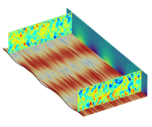
The experimental data of Hanratty et al. do not allow a comprehensive examination of all of the aspects regarding the perturbations due to the wall waviness. There are no available data on heat transfer at the wall. For applications, the analysis of the energy budget is determining since the wall regression is most often driven by transfers at the wall that can be represented without any loss of generality by heat transfer, as recalled in § 2.4. To access such data, DNS were conducted with the spectral difference Navier–Stokes solver named JAGUAR (Chapelier, Lodato & Jameson Reference Chapelier, Lodato and Jameson2016) and developed at ONERA and CERFACS. The code is designed to handle triangle (Veilleux et al. Reference Veilleux, Puigt, Deniau and Daviller2022a) or tetrahedral elements (Veilleux et al. Reference Veilleux, Puigt, Deniau and Daviller2022b) but all the presented computations were performed with a fourth-order discretisation scheme using hexahedral elements. Time integration is made with a low-dissipation low-dispersion sixth-order Runge–Kutta scheme. The computational domain is $[0,3\lambda ]\times [0,6\delta ]\times [\zeta _0\cos (\alpha x),\delta ]$ with $\alpha \delta ={{\rm \pi} }/{2}$. The streamwise extent of the domain is $12\delta \approx 4{\rm \pi} \delta$ that fits the usual requirements for periodic channel flow simulations. A constant source term is added on the momentum equation that sets the friction velocity $u_{\tau }$. The wall temperature is kept constant and the level of the mean heat flux on the wall is determined by the balance with the viscous and turbulent dissipation. As a consequence the wall heat flux is $\phi _w=\rho u_{\tau }^2 U_b$, with $U_b$ the bulk velocity, providing rather low values of $\phi _w^*=U_b^+$. Two mesh resolutions are used depending on the targeted Reynolds number. The numbers of solution points are $240\times 240 \times 160 \approx 9M$ and $320\times 320 \times 240 \approx 24M$. With a fourth-order discretisation, the mean $y^+$ values in the wall cells are found to stay between $0.25$ and $0.5$. The friction Reynolds numbers $\delta ^+$ range from $150$ to $500$ with $\mathcal {R}\in \{100,150,200,300\}$. Here again, the velocity field is nearly divergence free and the density fluctuations are several orders of magnitude lower than the velocity and pressure perturbations. The amplitude of the wall ripple is chosen to give $\zeta _0^+ \in [2.9,6.6]$, ensuring linear behaviours with $\alpha \zeta _0$ always less than $0.03$.

These DNS configurations cannot be directly considered as a complementary material to the experimental results of Hanratty et al. since $\alpha \delta$ is twice as small in the computations as in the experiments. However, it was shown in § 2.2 that, for $\mathcal {R}<500$, the phase shift $\psi _{\tau }$ is hardly affected by this change in the product $\alpha \delta$. This choice for $\alpha \delta$ is a compromise between representativeness and cost. The main purpose of these simulations is to serve as a reference for RANS computations and the linear analyses, especially concerning the heat transfer. For this reason, RANS computations were also performed with strictly similar conditions. All computations used air as the fluid with perfect gas assumptions and, given the temperature levels encountered, the specific heat capacity $C_p$ can be reasonably considered constant. The computed temperature fields are directly comparable to the enthalpy fields. We note by $\theta$ the temperature difference with the wall and $\theta ^+={\theta }/{\theta _{\tau }}$ the associated dimensionless variable, where $\theta _{\tau }={-\phi _w}/{\rho C_p u_{\tau }}$ is the friction temperature. Mean velocity profiles $\langle u^+ \rangle$ (figure 4) compare favourably between the different computations for all Reynolds numbers, even though the $k\unicode{x2013}\omega$ model underestimates the profiles in the buffer layer. The reference data of Hoyas & Jiménez (Reference Hoyas and Jiménez2008) obtained in non-deformed channels are also depicted to prove the validity of the DNS computations presented here. Second moments also agree between the two DNS datasets. The DNS mean temperature profiles are well reproduced by the EBRSM while the $k\unicode{x2013}\omega$ model tends to underpredict the profiles above the linear region.

Figure 4. Mean velocity (blue) and temperature (orange) profiles. Empty symbols ($\circ$,$\scriptstyle \square$) are DNS results while solid lines (EBRSM) and dashed lines ($k\unicode{x2013}\omega$) present RANS computations. The full black symbols ($\diamond$) are DNS results from Hoyas & Jiménez (Reference Hoyas and Jiménez2008) at $Re_{\tau }=180$ and $Re_{\tau }=550$: (a) ${\mathcal {R}}_{\tau }=150$; (b) ${\mathcal {R}}_{\tau }=300$.

4.1. Influence of the turbulent closures on RANS computations

The narrow differences in the mean quantities visible in figure 4 actually hide more vast discrepancies in the perturbation fields, which increase with the Reynolds number $\mathcal {R}$. Profiles of the velocity and temperature perturbation fields were extracted at several streamwise location ${x}/{\lambda }$ and plotted in figures 5 and 6. The amplitudes of the perturbation are divided by a factor $2$ when $\mathcal {R}$ is doubled, in accordance with the linear expansion (A4) stating that any quantity $q$ is such that ${(q^+-\langle q^+ \rangle )}/{\zeta _0^+} \propto \alpha ^+=\mathcal {R}^{-1}$. It is immediately apparent that the EBRSM compares better with the DNS results than the $k\unicode{x2013}\omega$ model. The agreement is better for velocity perturbations than for temperature perturbations, where a noticeable difference exists below $z^+=20$. Despite a good overall trend, the perturbation profiles presented by the $k\unicode{x2013}\omega$ model are lagged behind those of DNSs with smaller amplitudes. The higher the Reynolds number, the larger the lag. Another notable point that emerges from these figures is that the ordering between the profiles is modified from the centre of the channel to the wall. Figures 5 and 6 again illustrate the division between vortical and non-vortical regions. Around the centre of the channel, the phase of the perturbed field is not altered with respect to the wall and the ordering between profiles is aligned with the wall locations, i.e. in-phase or anti-phase, depending on the sign of the perturbation. Conversely, near the wall, the ordering is modified by the phase of the perturbed field. Moreover, DNS and RANS calculations have also revealed a perturbation peak in the velocity profiles around $z^+=10$, consistent with the vorticity peak revealed by the linear analysis (figure 3). A similar peak is also visible in the temperature profiles, but is less pronounced due to the high levels of perturbations observed in the non-vortical region. The wall shear stress disturbances ${(\tau _w^+-\langle \tau _w^+ \rangle )}/{\zeta _0^+}$ of figure 7 corroborate the previous observations with $k\unicode{x2013}\omega$ predictions delayed compared with those of DNS while the EBRSM provides better agreement. For the wall heat flux disturbances ${(\phi _w^+-\langle \phi _w^+ \rangle )}/{\zeta _0^+}$ presented in figure 7, the $k\unicode{x2013}\omega$ model underestimates the amplitudes and is not able to recover the phase shift. The EBRSM greatly improves the results but the phase shift on $\phi _w$ is a bit overpredicted. The RANS results for the wall shear stress phase $\psi _{\tau }$ are also reported in figure 2. The closure relations of the RANS computations are manifestly responsible for the prediction accuracy and the results evidence the failure of the Boussinesq hypothesis, as expected. Even though the wall deformation is very small, ensuring a linear behaviour of the perturbation, the flow field is heavily affected by the turbulent modelling. The error is even more pronounced on the perturbed temperature field and the wall heat flux. As explained above, the good behaviour of the EBRSM compared with the $k\unicode{x2013}\omega$ model is essentially due to the representation between the Reynolds stress difference $\overline {u'^2}-\overline {w'^2}$. Figure 8 shows the mean and disturbed profiles of $\overline {u'^2}^{~+}-\overline {w'^2}^{~+}$ and $-\overline {u'w'}^{~+}$ obtained with the EBRSM calculations compared with those from the DNS for $\mathcal {R}=300$. Although the forced response does not match that yielded by DNS, the profile of $\overline {u'^2}-\overline {w'^2}$ at leading order is in good agreement with DNS results, while for $k\unicode{x2013}\omega$ calculations, (not shown here) the normalised stress difference at the leading order is $\langle \overline {u'^2}^{~+}-\overline {w'^2}^{~+}\rangle =4\langle \nu _t ({\partial {u}}/{\partial {x}})\rangle =0$. Figure 8 also indicates that the perturbations due to the wall in the diagonal stress difference $\overline {u'^2}-\overline {w'^2}$ are four to five times larger than those induced in the shear stress $-\overline {u'w'}^{~+}$. The results show that the term ${\partial {(\tau _{xx}-\tau _{zz})}}/{\partial {x}}$ has a magnitude five times smaller than that of the term ${\partial {\tau _{xz}}}/{\partial {z}}$ in the streamwise momentum equation (A1). In the end, the ${\partial {(\tau _{xx}-\tau _{zz})}}/{\partial {x}}$ term contributes approximately 20 % in the budget of the momentum equation at the first order, showing its critical importance.

Figure 5. Profiles of velocity perturbations at stations $x/\lambda =0.0$ (blue), $x/\lambda =0.2$ (purple), $x/\lambda =0.4$ (green), $x/\lambda =0.6$ (orange) and $x/\lambda =0.8$ (red). Symbols are DNS results, solid lines present the RANS computations with the EBRSM while the dashed lines stand for the $k\unicode{x2013}\omega$ results: (a) ${\mathcal {R}}_{\tau }=150$; (b) ${\mathcal {R}}_{\tau }=300$.

Figure 6. Profiles of temperature perturbations. The legend is identical to that of figure 5: (a) ${\mathcal {R}}_{\tau }=150$; (b) ${\mathcal {R}}_{\tau }=300$.

Figure 7. Wall shear stress (left/blue colour) and wall heat flux disturbances (right/orange colour) at $\mathcal {R}=150$ (a) and $\mathcal {R}=300$ (b). Symbols are DNS results. Solid lines are the RANS computations with the EBRSM and the dashed lines represent the computations with the $k\unicode{x2013}\omega$ model.

Figure 8. (a) Mean profiles of the Reynolds stress difference $\overline {u'^2}^{~+}-\overline {w'^2}^{~+}$ (blue) and the shear stress $-\overline {u'w'}^{~+}$ (orange) for $\mathcal {R}=300$. Symbols are the DNS results and lines stand for the EBRSM computations. Corresponding forced responses profiles ${(\overline {u'^2}^{~+}-\overline {w'^2}^{~+}-\langle \overline {u'^2}^{~+}-\overline {w'^2}^{~+}\rangle )}/{\zeta _0^+}$ (b) and ${(-\overline {u'w'}^{~+}+\langle \overline {u'w'}^{~+}\rangle )}/{\zeta _0^+}$ (c) at several stations $x/\lambda$. Lines and symbols are those used in figure 5.

The RANS results are now used to further examine the results of the linear analysis and assess the effect of the Hanratty correction $\mathcal {C}$ on the prediction of the phase shift of the wall shear stress and the wall heat flux.

4.2. Achievements and limitations of the Hanratty correction

Previous work by Abrams & Hanratty (Reference Abrams and Hanratty1985), Charru et al. (Reference Charru, Andreotti and Claudin2013) and Claudin et al. (Reference Claudin, Duran and Andreotti2017) proved the effectiveness of the correction $\mathcal {C}$ in recovering the wall shear stress phase evolution with respect to the wavenumber (solid blue line in figure 2). Although very efficient, this correction suffers from two main limitations. The first one is related to the application of the correction in the mixing length model. The RANS computations highlighted the failure of the Boussinesq hypothesis to predict the stress difference $\tau _{xx}-\tau _{zz}$, which is then of the order of the perturbation $O(\alpha \zeta _0)$, in the streamwise momentum equation (A1). However, the Hanratty correction acts on the shear stress $\tau _{xz}$ through the modification of the mixing length. In other words, the Hanratty correction does not correct the problematic term but balances the streamwise momentum equation, and, in that sense, it can be viewed as an ad hoc palliative to the failure of the Boussinesq hypothesis. The second limitation comes from the use of a relaxed pressure gradient to drive the correction $\mathcal {C}$. The RANS and DNS calculations have evidenced the role of the mean vorticity of the flow in creating the turbulent stresses that ultimately lead to the observed phase shift in the wall shear stress. However, the pressure gradient does not enter the vorticity equation and is not a relevant variable to control turbulence. Furthermore, the pressure gradient is not involved in the Reynolds stress transport equations, which does not prevent the EBRSM computations from correctly reproducing the phase shift of the wall shear stress. Despite these limitations, the Hanratty correction is very useful and effective for linear analyses.

A further demonstration of the positive impact of the correction $\mathcal {C}$ is shown in figure 9, where the amplitudes of the wall shear stress disturbance are presented. In the linear analysis the wall shear stress fluctuation ${(\tau _w^+-\langle \tau _w^+ \rangle )}/{\zeta _0^+}$ is given by $\alpha \hat {\tau }_{xz}(0)$ according to (A4). Calculations of the linear response with $\mathcal {C}$ and, to a lesser extent, the EBRSM results, follow the measurements remarkably well, while the $k\unicode{x2013}\omega$ model and results of the linear analysis without the Hanratty correction move further apart as $\alpha ^+$ is decreased. We now focus on the use of the Hanratty correction in the closure relation for turbulent heat flux of the linearised energy equation detailed in § (2.4). In the mixing length disturbance $\hat {l}_{\theta }$ (2.5), $\mathcal {C}$ is considered twice with respect to the two van Driest numbers $A$ and $A_{\theta }$. An additional dependence on $\hat {\tau }_{xz}$ was introduced for the van Driest number $A_{\theta }$. Best agreements were obtained with $\epsilon _{\theta }=4$. The results of the linear analysis for the evolution of the phase of the wall heat flux $\psi _{\phi }$ with respect to $\alpha ^+$ are shown in figure 10 and compared with RANS computations. Results corresponding to the original model proposed by Claudin et al. (Reference Claudin, Duran and Andreotti2017) ($A_{\theta }=26$ and $\epsilon _{\theta }=0$) are also reported in figure 10. Values of $\psi _{\phi }$ are shifted from $180^{\circ }$ when the sign of $\phi _w^*$ is changed. When $\vert \phi _w^* \vert$ is large enough, practically when $\vert \phi _w^* \vert >100$, the dissipation term $\hat {u}$ of the equation for the mean enthalpy (A14) is almost negligible and the equation is symmetrical with respect to $\phi _w^*$. The Navier–Stokes computations with the $k\unicode{x2013}\omega$ model provide values of $\psi _{\phi }$ in good agreement with the linear analysis obtained with the frozen turbulence assumption, consistent with the observation made on $\psi _{\tau }$ in figure 2. Results equivalent to those of Claudin et al. (Reference Claudin, Duran and Andreotti2017) provide overestimated phase values of approximately $40^{\circ }$ whereas, with $A_{\theta }^0=30$ and especially $\epsilon _{\theta }=4$, the linear forced responses match those of the EBRSM computations. This means that the Hanratty correction has a beneficial impact on $\hat {l}_{\theta }$ but it is not sufficient. An additional correction on $A_{\theta }$, with $\epsilon _{\theta }=4$, is required to recover the results obtained with the EBRSM computations.

Figure 9. Amplitude of the wall shear stress perturbation. The filled black circles are measurements of Hanratty et al.. Square symbols are the RANS computations with the EBRSM (blue) and the $k\unicode{x2013}\omega$ (orange) model. The solid lines are the results of the linear analysis with the Hanratty correction (blue) and when the frozen turbulence assumption is used (orange).

Figure 10. Wall heat flux disturbance phase $\psi _{\phi }$ as a function of the wavenumber $\alpha ^+$. Blue symbols are the phase computed with the EBRSM for $\phi _w^*=400$ ($\Diamond$) and $\phi _w^*=-400$ ($\square$). The orange square symbols are the results obtained with the $k\unicode{x2013}\omega$ model. The solid lines are the corresponding results of the linear analysis with (blue line) all corrections activated ($A=26$, $A_{\theta }=30$, $\beta =35$, $\epsilon _{\theta }=4$) and with (orange line) the frozen turbulence hypothesis ($A=26$, $A_{\theta }=30$, $\beta =0$, $\epsilon _{\theta }=0$). The black dashed line presents the results corresponding to the approach followed by Claudin et al. (Reference Claudin, Duran and Andreotti2017) for $l_{\theta }$ ($A=26$, $A_{\theta }=26$, $\beta =35$, $\epsilon _{\theta }=0$). The thin horizontal dashed line corresponds to $\psi _{\phi }=-90^{\circ }$.

In figure 11 the comparison of the amplitude of the wall heat flux disturbance points out several divergences. The disturbances of the wall heat flux ${(\phi _w^+-\langle \phi _w^+ \rangle )}/{\zeta _0^+}$ obtained in the linear analysis, i.e. $-\alpha \hat {f}(0)$, are smaller than those of the RANS computations. The results produced by the $k\unicode{x2013}\omega$ model and the results of the linear analysis with the frozen turbulence assumption exhibit almost the same trends whereas the EBRSM and the linear analysis results diverge as $\alpha ^+$ decreases. This may be due to the closure relation used for the turbulent heat fluxes $-\overline {u_i'h'}$. The EBRSM uses the GGDH assumption while the linear analysis makes use of a SGDH hypothesis and is impacted by the Hanratty correction $\mathcal {C}$ in $\hat {l}_{\theta }$ (2.5). The results obtained with $A_{\theta }^0=26$ and $\epsilon _{\theta }=0$ are not better. For the energy equation, the Hanratty correction is not able to compensate the approximation made in the modelling of the turbulent heat fluxes. This is not surprising since $\mathcal {C}$ was implicitly designed to correct only for the misrepresentation of the Reynolds stresses. Although imperfect, the linear analysis using the model described in § 2.4 for the energy equation allows a good prediction of $\psi _{\phi }$. However, it was not possible with this type of closure (2.5) for $\hat {l}_{\theta }$ to also obtain a satisfying prediction of the wall heat flux amplitude.

Figure 11. Amplitude of the wall heat flux perturbation. Square symbols are the RANS computations with the EBRSM (blue) and the $k\unicode{x2013}\omega$ (orange) model. The solid and dashed lines are the results of the linear analysis. The blue lines correspond to results of the linear approach with $\phi _w^*=400$ (dashed) and $\phi _w^*=-400$ (solid). The orange line presents the analysis performed with the frozen turbulence assumption. The dashed black line shows the results obtained with $A_{\theta }=A_{\theta }^0=26$ and $\epsilon _{\theta }=0$.

4.3. Linear stability of an ablative surface

The surface elevation is now a function of time $\zeta (x,t)=\zeta _0 \exp ({ (\sigma _w t+ {\rm i}\omega _w t + {\rm i}\alpha x)})$ and is assumed to be ruled by the ablation process and controlled by the wall heat flux. For moving surfaces, the critical layer, below which the flow propagates more slowly than the surface, has a crucial importance on the flow dynamics (Belcher & Hunt Reference Belcher and Hunt1998). For our re-entry applications (see Appendix B), the surface speed ${\omega _w}/{\alpha }$ is low compared with the friction velocity. In this slow waves regime (${\omega _w}/{\alpha u_{\tau }}\lesssim 15$) the critical layer is thin and plays no significant dynamical role. In other words, only the temporal growth rate $\sigma _w$ matters and controls the surface regression in direction $z$.

The model detailed in the Appendix A.2 can be applied to dissolution or melting problems since the energy equation produces similar results to the advection–diffusion equation used by Claudin et al. (Reference Claudin, Duran and Andreotti2017) when $\vert \phi _w^* \vert$ is large. Any solid surface can be decomposed into a series of sinusoidal profiles and the linear response of the flow will be the combination of the responses for each wavenumber. The surface regression is assumed to be proportional to the wall flux (Claudin et al. Reference Claudin, Duran and Andreotti2017). Dropping the homogeneous part of the flux, the evolution of the elevation at the first order is ruled by ${\partial {\zeta }}/{\partial {t}}=-r u_{\tau }^3 \zeta _0 \alpha \vert \hat {f}(0) \vert \exp ({ ({\rm i}\alpha x+{\rm i}\psi _{\phi })})$, with $r$ a constant proportionality factor (s$^{2}$/m$^{2}$), controlling the regression rate. The temporal growth rate of the surface elevation is then governed by the real part of the dispersion relation, i.e. $\sigma _w=-r u_{\tau }^3 \alpha \vert \hat {f}(0) \vert \cos (\psi _{\phi })$. Function $\sigma _w(\alpha )$ changes sign when $\vert \psi _{\phi } \vert$ crosses the horizontal line $\psi _{\phi }=90^{\circ }$. In the case of a negative wall heat flux, the horizontal line $\psi _{\phi }=-90^{\circ }$ is plotted in figure 10. When the Boussinesq hypothesis is used without the Hanratty correction in the linear analysis and for the computations with the $k\unicode{x2013}\omega$ model, $\psi _{\phi }$ is always less than $-90^{\circ }$ and $\sigma _w$ remains negative for all wavenumbers $\alpha ^+$. For the EBRSM results or for the linear responses involving the correction $\mathcal {C}$, $\sigma _w$ becomes positive for $\alpha ^+\approx 0.006$. All wavenumbers below $\alpha ^+ \approx 0.006$ are unstable, in the range of wavenumbers covering the transitional regime. However, the growth rate $\sigma _w$ quickly decreases as $\alpha ^+$ decreases, mainly due to its proportionality with $\alpha$. In figure 12, growth rates $\sigma _w$ (normalised) obtained in the RANS computations and in the linear analysis are depicted with respect to $\alpha ^+$. In the $k\unicode{x2013}\omega$ computations and in the linear analysis with the frozen turbulence assumption, the growth rates are always negative. Both models predict stable modes regardless of $\alpha ^+$. But the EBRSM and the linear approach show an unstable region where $\sigma _w>0$ and the presence of a peak. The wavenumber associated with this peak indicates the most unstable mode for which the surface time growth rate is the highest. The error in the prediction of the amplitude of the wall heat flux with the linearised model using (2.5) for the closure of the turbulent heat flux leads to a shift in the position of the peak. The linear analysis indicates a peak at $\alpha ^+=2.4 \times 10^{-3}$ ($\mathcal {R}= 417$) whereas it is found at $\alpha ^+\approx 4\times 10^{-3}$ ($\mathcal {R}=250$) by the EBRSM. The location of the peak is almost independent of $\phi _w^*$ and is not modified by the sign of $\phi _w^*$ as long as $\vert \phi _w^* \vert > 100$. The Prandtl number $Pr$ has a limited influence on the peak position in the linear approach. The same tendency is expected in Navier–Stokes computations. The peak is moved to higher values of $\alpha ^+$ as $Pr$ is increased and, for example, when $Pr=100$, the peak is located at $\alpha ^+=4.2\times 10^{-3}$.

Figure 12. Normalised growth rate ${\sigma _w \phi _w}/{r\rho }$ with respect to $\alpha ^+$ in logarithmic and linear scales. Square symbols are the RANS computations with the EBRSM (blue) and $k\unicode{x2013}\omega$ (orange) model. The corresponding dashed lines are splines computed from the data. The solid lines are the results of the linear approach with (orange) and without the frozen turbulence assumption.

Thomas (Reference Thomas1979) presented evidence in support of the hypothesis that the scalloping of soluble surfaces may be attributed to wall turbulence. By analysing bed morphologies where scallops occur, he showed that the longitudinal wavelength of the bedform is a multiple of the viscous length $\delta _{\nu }$ providing $\alpha ^+ \approx 6\times 10^{-3}$. The proportionality between these quantities was demonstrated over a range exceeding four decades of length and covering a wide variety of situations from the corrosive dissolution of steel (Schoch Reference Schoch1968; Schoch, Richter & Köhle Reference Schoch, Richter and Köhle1969; Schoch, Richter & Effertz Reference Schoch, Richter and Effertz1970a; Schoch et al. Reference Schoch, Wiehn, Richter and Schuster1970b; Schuster Reference Schuster1971; Heimsch et al. Reference Heimsch, Hegele, Pfau, Bursik, Richter and Welter1978), brass (Sick Reference Sick1972) and copper (Knutsson, Mattsson & Ramberg Reference Knutsson, Mattsson and Ramberg1972), the plastic shear of bitumen (Brauer Reference Brauer1963) and aluminium (Brunton Reference Brunton1966) and the rippling of colloidal-particle deposits in a water main (Wiederhold Reference Wiederhold1949; Seiferth & Krüger Reference Seiferth and Krüger1950). In the context of atmospheric re-entry vehicles, the wavelength found in the TATER experiment (Hochrein & Wright Reference Hochrein and Wright1976) aligns with the Thomas correlation. The orders of magnitude provided in Appendix B justify the use of the linear approach (A.1 and A.2) to study this type of flow, particularly with respect to compressibility effects. The location of the most unstable mode with the EBRSM computations or with the linear approach are closed to the value found in the Thomas correlation, confirming the role of turbulence in the occurrence of scallops. It is nevertheless premature to draw general conclusions from these results. Only the linear response was examined, with a high degree of hypothesis on the flow that restricts the scope of the approach. Further verification is needed to extend the approach to different types of erodible surfaces where scallops are observed. Nonlinear effects, notably related to flow separations, may also interfere in the scallop formation (Charru et al. Reference Charru, Andreotti and Claudin2013). This will certainly require further experimental or numerical data for validation. The results presented are a first step towards explaining the value of the slope of the Thomas correlation.