


1. Introduction
Thermal convection is ubiquitous in natural and engineered systems (Ahlers, Grossmann & Lohse Reference Ahlers, Grossmann and Lohse2009; Lohse & Xia Reference Lohse and Xia2010; Stevens, Clercx & Lohse Reference Stevens, Clercx and Lohse2013). For example, convection plays a dominant role in many solar energy flat-plate collectors (Das, Roy & Basak Reference Das, Roy and Basak2017), and heat transfer from the core to the exterior of stellar structures is of paramount importance (Long et al. Reference Long, Mound, Davies and Tobias2020). In such flows, the fluid motion is driven by buoyancy forces that arise from density variations owing to thermal gradients, and the flows can be classified based on the relative directions of the imposed temperature gradient and gravity (Das et al. Reference Das, Roy and Basak2017). Some studies have considered flows where the temperature gradient is perpendicular to gravity (Basak et al. Reference Basak, Roy, Sharma and Pop2009a,Reference Basak, Roy, Singh and Pandeyb, Reference Basak, Roy, Singh and Pop2010; Hussam & Sheard Reference Hussam and Sheard2013), but perhaps the most commonly studied situation is where the temperature gradient is parallel to gravity, such as in Rayleigh–Bénard convection (RBC). However, in many real world circumstances, the imposed temperature gradient is neither parallel nor perpendicular to gravity (Bejan Reference Bejan2013). Such situations can occur for thermal convection inside enclosures with irregular geometries, which have been reviewed in detail recently by Das et al. (Reference Das, Roy and Basak2017). Among the many different possible geometries, thermal convection on a spherical surface is an interesting model for studying astrophysical and geophysical flows (Kellay Reference Kellay2017), and this is the subject of the present work.
Two key parameters that determine the behaviour of a (non-rotating) thermally convective flow are the Rayleigh number,  $Ra$ and the Prandtl number $Pr$. The $Ra$ characterises the ratio of the time scale between diffusive and convective thermal transport; the $Pr$ is the ratio of momentum diffusivity to thermal diffusivity. Given $Ra, Pr$, two other emergent parameters in the flow that are of utmost importance are the Reynolds number $Re$ and the Nusselt number $Nu$, with $Re$ denoting the ratio of inertial force to viscous force and $Nu$ characterising the heat transport properties of the flow.
The RBC is an important model for the study of the turbulent thermal convection, and can be implemented conveniently in experiments or numerical simulations (Ahlers et al. Reference Ahlers, Grossmann and Lohse2009; Lohse & Xia Reference Lohse and Xia2010; Stevens et al. Reference Stevens, Clercx and Lohse2013). Research on RBC may be broadly described in terms of two aspects: the small-scale and large-scale dynamics. The study of the small-scale properties has tended to focus on the scaling of velocity and temperature structure functions, and intermittent behaviour in the flow. A recent review of the small-scale properties can be found in the work of Lohse & Xia (Reference Lohse and Xia2010). Studies on the large-scale properties of RBC tend to focus on exploring the dependence of the emergent properties  $Nu$ and $Re$ on the control parameters $Ra$ and $Pr$, as well as the properties of thermal plumes and large-scale circulations (LSC). A detailed discussion of theoretical and experimental progress on RBC can be found in Ahlers et al. (Reference Ahlers, Grossmann and Lohse2009).
In geophysical and astrophysical flows, convectively driven flows are also influenced by system rotation, e.g. owing to planetary rotation. Rotating RBC (RRBC) is often considered a suitable model for studying such flows where both buoyancy and rotation play important roles (Stevens et al. Reference Stevens, Clercx and Lohse2013). In RRBC the Rayleigh–Bénard system rotates about the direction parallel to gravity (the vertical direction), and when considered in a rotating frame of reference, rotation is seen to introduce centrifugal and Coriolis forces to the dynamical system. For RRBC another important control parameter is the Rossby number,  $Ro$. When $Ro\gg 1$ the effect of rotation on the flow is weak, while it is strong for $Ro\ll 1$.
An early experimental study on RRBC was performed by Rossby (Reference Rossby1969) in a cylindrical vessel. This study showed that the onset of convection is delayed by rotation (Rossby Reference Rossby1969), something that was studied in more detail in Zhong, Ecke & Steinberg (Reference Zhong, Ecke and Steinberg1993), and also that the heat flux in the flow could be increased by up to  $10\,\%$ owing to the presence of rotation. Since the work of Rossby (Reference Rossby1969), further research on cylindrical vessel flows with varying aspect ratios $\varGamma$ have shown that with the increase of $1/Ro$, RRBC goes through three successive regimes: the weak rotation regime, the moderate rotation regime and the strong rotation regime (Kunnen et al. Reference Kunnen, Stevens, Overkamp, Sun, van Heijst and Clercx2011; Stevens et al. Reference Stevens, Clercx and Lohse2013), which are denoted by regime I, II and III, respectively.
In regime I, the rotation is too weak to interfere with the flow structures and the heat flux is essentially independent of the rotation because the rotationally induced forces are negligible compared to buoyancy (King, Stellmach & Buffett Reference King, Stellmach and Buffett2013). In this regime, LSC are the prominent flow structures and  $Nu$ does not vary with $Ro$ (Weiss & Ahlers Reference Weiss and Ahlers2011b,Reference Weiss and Ahlersa).
In regime II, the system depends on the interaction between the rotationally induced forces and buoyancy. Small vertical plumes parallel to the rotation axis take the place of LSC as the dominant flow structures, while heat transport is enhanced with decreasing  $Ro$ (Boubnov & Golitsyn Reference Boubnov and Golitsyn1986; Sakai Reference Sakai1997; Vorobieff & Ecke Reference Vorobieff and Ecke2002; Kunnen, Geurts & Clercx Reference Kunnen, Geurts and Clercx2010; Scheel, Mutyaba & Kimmel Reference Scheel, Mutyaba and Kimmel2010; Weiss & Ahlers Reference Weiss and Ahlers2011b; King, Stellmach & Aurnou Reference King, Stellmach and Aurnou2012; Guervilly, Hughes & Jones Reference Guervilly, Hughes and Jones2014; Horn & Shishkina Reference Horn and Shishkina2015; Zhong, Sterl & Li Reference Zhong, Sterl and Li2015). In this regime, variations of the flow in the vertical direction can suppressed owing to the well known Taylor–Proudman effect. However, the vertical plumes also convey hot fluid from the Ekman layer to the cold bulk of the fluid, a phenomenon referred to as ‘Ekman pumping’. This pumping causes $Nu$ to increase with decreasing $Ro$ in regime II. Zhong & Ahlers (Reference Zhong and Ahlers2010) and Stevens et al. (Reference Stevens, Zhong, Clercx, Ahlers and Lohse2009) have studied the transition where the flow enters regime II by $1/Ro$ passing its critical value $1/Ro_{c}$. Zhong et al. (Reference Zhong, Stevens, Clercx, Verzicco, Lohse and Ahlers2009) studied the dependence of the heat-flux enhancement owing to rotation on $Ra$ and $Pr$, and shows that when $Pr$ is large and $Ra$ is relatively small, enhancements of up to $30\,\%$ are possible. However, they showed that for sufficiently small $Pr$ the enhancement vanishes. Furthermore, they showed that increasing $Ra$ also reduces the enhancement. Zhong & Ahlers (Reference Zhong and Ahlers2010) also showed that that the critical non-dimensional rotation rate $1/Ro_{c}$ required for the flow to enter regime II is reduced by increasing $Pr$ and is not affected by $Ra$ in the parameter range concerned by their study.
In regime III,  $Ro$ is small enough such that the rotationally induced forces dominate the system and $Nu$ plunges as $Ro$ is further decreased (Rossby Reference Rossby1969; Zhong et al. Reference Zhong, Ecke and Steinberg1993; Liu & Ecke Reference Liu and Ecke1997; Vorobieff & Ecke Reference Vorobieff and Ecke2002; Kunnen, Clercx & Geurts Reference Kunnen, Clercx and Geurts2006, Reference Kunnen, Clercx and Geurts2008; Zhong et al. Reference Zhong, Stevens, Clercx, Verzicco, Lohse and Ahlers2009). In this regime, turbulence is quenched and the efficiency of heat transport is greatly diminished. The heat flux experiences a sharp drop owing to the Taylor–Proudman effect in regime III. Vorobieff & Ecke (Reference Vorobieff and Ecke2002) discovered that near the top and bottom boundaries cyclonic vortices collect that are aligned with the rotation axis. The same phenomenon appears not only in the experiments of Sakai (Reference Sakai1997) and Boubnov & Golitsyn (Reference Boubnov and Golitsyn1986) but also in the numerical simulations of Julien et al. (Reference Julien, Legg, Mcwilliams and Werne1996). Grooms et al. (Reference Grooms, Julien, Weiss and Knobloch2010) specified these cyclonic vortices as convective Taylor columns and developed a nonlinear model of these flow structures. Furthermore, in the study of Guervilly et al. (Reference Guervilly, Hughes and Jones2014), these cyclonic vortices were shown to be large scale and posses a long lifetime when $Ra$ and $1/Ro$ are large enough. In the study of King et al. (Reference King, Stellmach, Noir, Hansen and Aurnou2009), regime III is argued to emerge when the Ekman boundary layer become thinner than the thermal boundary layer. Horn & Shishkina (Reference Horn and Shishkina2015) decomposed the velocity field into toroidal and poloidal components to understand the differences between the three regimes, while Rajaei et al. (Reference Rajaei, Alards, Kunnen and Clercx2018) considered the transition between the regimes using statistical analysis of the turbulent velocity fields.
Many studies have focused on the scaling properties of the heat flux, such as the behaviour of the scaling exponent  $\xi$ in the relation $Nu\sim Ra^{\xi }$. The first unifying theoretical attempt is achieved by Malkus & Chandrasekhar (Reference Malkus and Chandrasekhar1954). In his work, $\xi$ is deduced to be $1/3$ using a hypothesis based on the self-adapted thickness of thermal boundaries. However, the theory of Malkus & Chandrasekhar (Reference Malkus and Chandrasekhar1954) lacks a formulation of the relation between $Nu$ and $Pr$. There are also other theoretical efforts made by Castaing et al. (Reference Castaing, Gunaratne, Heslot, Kadanoff, Libchaber, Thomae, Wu, Zaleski and Zanetti1989) and Cioni, Ciliberto & Sommeria (Reference Cioni, Ciliberto and Sommeria1997), which are based on the model of the mixing zone. They proposed a scaling behaviour of $\xi =2/7$. Meanwhile, the same scaling coefficient is obtained by Shraiman & Siggia (Reference Shraiman and Siggia1990) with a very different hypothesis. Julien et al. (Reference Julien, Legg, Mcwilliams and Werne1996) showed that $\xi =2/7$ when boundaries are stress-free, while no-slip boundaries give $\xi =1/3$. Pharasi et al. (Reference Pharasi, Kannan, Kumar and Bhattacharjee2011) showed that for stress-free boundaries, when $Pr=0.1$, $\xi =2/7$ only if $Nu$ exceeds a critical value. King et al. (Reference King, Stellmach and Aurnou2012) showed that in regime III $Nu=(Ra/Ra_c)^{3}$, where $Ra_c$ is the critical $Ra$ for the onset of convection. Grossmann & Lohse (Reference Grossmann and Lohse2000, Reference Grossmann and Lohse2001, Reference Grossmann and Lohse2002, Reference Grossmann and Lohse2004) have established the unifying theory which succeeded in the prediction of $\xi$ in a wide range of $Ra$ and $Pr$. The GL theory unifies the formulas of $\xi$ and agrees well with the most of the experimental results. One of the most significant insights offered by the Grossmann–Lohse (GL) theory is to develop the kinetic and thermal dissipation rate $\epsilon _{U}$ and $\epsilon _{T}$ into boundary components and bulk components, respectively (i.e. $\epsilon _{U} = \epsilon _{U,BL} + \epsilon _{U,bulk}$ and $\epsilon _{T} = \epsilon _{T,BL} + \epsilon _{T,bulk}$). The two fundamental premises of GL theory have already been validated by the experiments (Xia, Lam & Zhou Reference Xia, Lam and Zhou2002; Funfschilling et al. Reference Funfschilling, Brown, Nikolaenko and Ahlers2005). The first premise is the existence of large-scale circulation in the flow (Xi, Lam & Xia Reference Xi, Lam and Xia2004). The second is that both the velocity and temperature boundaries satisfy the Prandlt–Blasius laminar hypothesis (Quan et al. Reference Quan, Stevens, Sugiyama, Grossmann, Lohse and Xia2010; Zhou & Xia Reference Zhou and Xia2010). Using both premises, the formula of $\epsilon _{U,BL}$, $\epsilon _{U,bulk}$, $\epsilon _{T,BL}$ and $\epsilon _{T,bulk}$ is evaluated through dimensional analysis. Moreover, $\epsilon _{U}$ and $\epsilon _{T}$ are explicitly linked to $Nu$,
$Nu$,  $Ra$ and $Pr$. As a result, $Nu(Ra,Pr)$ is obtained by an implicit equation of $Nu$,
$Nu$,  $Ra$ and $Pr$. However, the experimental results indicate that the rotation of thermal convection have little impact on $\xi$ (King et al. Reference King, Stellmach and Aurnou2012).
In RRBC, the centrifugal force contributes in two ways. Part of the contribution would exist even in the absence of temperature variations throughout the flow, and this contribution may be absorbed into the pressure gradient term. The other contribution is a centrifugal buoyancy force that is associated with density fluctuations. As noted in Horn & Aurnou (Reference Horn and Aurnou2018), most previous direct numerical simulation (DNS) studies have ignored this centrifugal buoyancy force, sometimes motivated by simplicity (because there are many other complex aspects of RRBC that are already yet to be understood even without this additional effect) and sometimes motivated by the fact that in some parameter regimes it may be appropriate to neglect centrifugal buoyancy force under Boussinesq-type approximations. However, Scheel et al. (Reference Scheel, Mutyaba and Kimmel2010) performed DNS that included the centrifugal buoyancy force and showed that it was necessary in order to explain the square patterns discovered in the experiments of RRBC, and Horn & Aurnou (Reference Horn and Aurnou2018) and Horn & Aurnou (Reference Horn and Aurnou2019) conducted DNS including this force and showed that it can play an important role.
Recently, an alternative system has been explored in order to understand turbulent motion and heat transfer on a curved surface, namely Kellay's soap bubble (Kellay Reference Kellay2017), which has yielded interesting results on the behaviour of turbulent convection, as well as a model for hurricane tracking (Seychelles et al. Reference Seychelles, Amarouchene, Bessafi and Kellay2008, Reference Seychelles, Ingremeau, Pradere and Kellay2010; Meuel et al. Reference Meuel, Xiong, Fischer, Bruneau, Bessafi and Kellay2013, Reference Meuel, Coudert, Fischer, Bruneau and Kellay2018). In Kellay's experiment, a half soap bubble (hemisphere) is heated from its equator, producing buoyancy forces and convection, resulting in a quasi-two-dimensional flow on a hemispherical surface. Unlike standard RBC, the local buoyancy force in this flow varies with location not only because of variations in the local fluid temperature, but also because the component of gravity acting on the flow varies with latitude on the bubble. In Bruneau et al. (Reference Bruneau, Fischer, Xiong and Kellay2018), DNS of the soap bubble showed  $Re$ and $Nu$ as a function of $Ra$ and found scaling behaviour that is remarkably similar to that found in standard RBC. In Meuel et al. (Reference Meuel, Coudert, Fischer, Bruneau and Kellay2018) the system was further explored by subjecting the soap bubble to rotation. Unlike RRBC, in the rotating soap-bubble flow, the effect of the Coriolis force varies with location owing to geometrical reasons, being zero at the equator of the bubble. Significant effects of the rotation were found on the structure functions of velocity and temperature in Meuel et al. (Reference Meuel, Coudert, Fischer, Bruneau and Kellay2018).
The study of Meuel et al. (Reference Meuel, Coudert, Fischer, Bruneau and Kellay2018) only rather briefly explored the properties of the flow on the rotating soap bubble, and there is much to understand about this flow, and the various ways in which its properties are similar and dissimilar to RRBC. Such a detailed study is the goal of this present paper. The outline of the paper is as follows. In § 2, the equations of motion for the system, their properties and non-dimensional parameters are discussed, as well as the DNS used to solve the equations. In § 3 we explore the single-point properties of the flow, including the behaviour of  $Re, Nu$, the mean flow and Reynolds stresses. In § 4 we explore the properties of the flow at different scales, considering fluxes of kinetic energy, enstrophy and thermal energy. Structure functions of the velocity and temperature field are also explored, along with a detailed consideration of their scaling behaviour. Finally, in § 5 we draw conclusions of the work and discuss future directions for study.
2. Governing equations and DNS
2.1. Governing equations and control parameters
We consider the flow of a half soap bubble of radius  $R$ that is heated from its equator, replicating the experimental set-up of Kellay (Reference Kellay2017). The bubble geometry is such that its thickness is negligible compared to its radius, and the flow in the radial direction has little effect on the heat and mass transfer of the system. Therefore, the system may be modelled as a two-dimensional flow on a hemispherical surface of radius $R$, with boundary conditions applied at the equator. Furthermore, we consider a system where the bubble rotates at a rate $\varOmega \equiv \|\boldsymbol {\varOmega }\|$ about its north pole.
The bubble may be described in terms of the three-dimensional Cartesian coordinate system, with coordinates  $(x,y,z)$ and unitary basis vectors $\boldsymbol {e_x},\boldsymbol {e_y},\boldsymbol {e_z}$. With respect to this, the bubble under consideration has its equator on the $(x,y,z=0)$ plane, and rotates about $\boldsymbol {e_z}$, with $\boldsymbol {e_z}\boldsymbol {\cdot } \boldsymbol {\varOmega }=\varOmega$. Given the curved surface of the bubble, it is also convenient to use a geographical coordinate system with coordinates $(r,\theta ,\phi )$, and basis vectors $\boldsymbol {e_{r}}(\theta ,\phi ),\boldsymbol {e_{\theta }}(\theta ,\phi ),\boldsymbol {e_{\phi }}(\theta ,\phi )$, where $\boldsymbol {e_{r}}(\theta ,\phi )\times \boldsymbol {e_{\theta }}(\theta ,\phi )=\boldsymbol {e_{\phi }}(\theta ,\phi )$. The latitudinal coordinate $\theta \in [0,{\rm \pi} ]$ increases from 0 at the equator, and the longitudinal coordinate is $\phi \in [0,2{\rm \pi} )$. In these coordinates, the two-dimensional flow is on the surface $(r=R,\theta ,\phi )$, and there is no flow in the direction $\boldsymbol {e_{r}}(\theta ,\phi )$.
The two-dimensional flow on the hemisphere is governed by the incompressible Navier–Stokes equations with the Oberbeck–Boussinesq approximation
 \begin{gather} \frac{\textrm{D}\boldsymbol{U}}{\textrm{D}t} ={-}\frac{1}{\rho}\boldsymbol{\nabla} p+\nu\triangle\boldsymbol{U} - \beta T \boldsymbol{g} - 2\boldsymbol{\varOmega}\times\boldsymbol{U} - F\boldsymbol{U}, \end{gather}
 \begin{gather}\boldsymbol{\nabla}\boldsymbol{\cdot}\boldsymbol{U}=0, \end{gather}
 \begin{gather}\frac{\textrm{D}T}{D\rm{}t} = \alpha\triangle T - ST, \end{gather}
where  $\boldsymbol {U}$ is the velocity field, $p$ is the pressure field, $T$ is the temperature field, $\nu$ is the kinematic viscosity, $\alpha$ is coefficient of thermal diffusion, $\beta$ is the coefficient of thermal expansion and $\rho$ is the constant reference density. We consider the case where gravity and rotation are aligned with $\boldsymbol {e_z}$, and $\boldsymbol {e_z}\boldsymbol {\cdot } \boldsymbol {g}=-g$. As discussed in the introduction, centrifugal buoyancy can play a role in the dynamics of rotating, convective turbulence. However, as with most studies on RRBC, we choose to neglect its effect here for simplicity, in order to first understand the role of the Coriolis force on the bubble flow. The part of the centrifugal force that is not associated with the background density field is, however, accounted for through the pressure term via the incompressibility constraint.
Boundary conditions are applied on the hemisphere equator, with no-slip for the velocity and a fixed value for the temperature field. Buoyancy driven flow on the hemisphere is therefore fundamentally different to the classical Rayleigh–Bénard systems for which there is a boundary through which heat flows out. In Kellay's heated soap bubble experiment (Kellay Reference Kellay2017), part of the energy is lost through exchange with the cold air outside and inside the bubble. The terms in (2.1) and (2.3) involving  $S$ and $F$ are supposed to represent this energy loss to the surrounding air. Related to this, these terms are also included in order to generate a non-trivial steady-state flow, because without the friction term in the momentum equation, the inverse energy cascade would lead to the formation of large-scale structures on to which energy continues to accumulate. The momentum friction term is therefore include to arrest the inverse cascade, allowing for a steady-state turbulent flow, analogous to the way in which DNS of two-dimensional turbulence uses a friction term to prevent accumulation of energy at the large scales of the flow (Boffetta & Ecke Reference Boffetta and Ecke2012). For the temperature equation, the boundary condition we are using is such that in the absence of a cooling term in (2.3), the temperature of the flow would continue to rise until it equals that on the boundary. In such a state, there would be no temperature gradients or fluctuations, and so no convection or turbulence. Therefore, a cooling term is required in (2.3) in order to generate a non-trivial steady state. We will return momentarily to discuss the specification of $S$ and $F$. Concerning the initial conditions for the system, the initial temperature of the bubble is the same as the surrounding air, and the velocity is initially zero everywhere.
In order to define the various control parameters in the system, we take the characteristic length to be the radius of the bubble  $R$, and the temperature difference $\delta T$ to be the difference in temperature between the equator and the cold air surrounding the bubble. Using these, we define the Raleigh number $Ra$, Rossby number $Ro$ and Prandtl number $Pr$ as follows:
 \begin{gather} Ra \equiv \frac{g\beta R^{3} \delta T}{\nu \alpha}, \end{gather}
 \begin{gather}Ro \equiv \frac{\sqrt{g/R}}{2\varOmega}, \end{gather}
 \begin{gather}Pr \equiv \frac{\nu}{\alpha}. \end{gather}
On the bubble, the velocity field may be represented as
 \begin{equation} \boldsymbol{U} = U_{\theta}\boldsymbol{e_{\theta}}+U_{\phi}\boldsymbol{e_{\phi}}, \end{equation}
where  $U_\theta \equiv \boldsymbol {e_{\theta }}\boldsymbol {\cdot } \boldsymbol {U}$, $U_\phi \equiv \boldsymbol {e_{\phi }}\boldsymbol {\cdot } \boldsymbol {U}$, while for the radial direction, $U_r\equiv \boldsymbol {e_r} \boldsymbol {\cdot } \boldsymbol {U}=0$ because the flow is two-dimensional. We also define the fluctuations $\boldsymbol {U}'\equiv \boldsymbol {U}-\langle \boldsymbol {U}\rangle$ with components $U_\theta '\equiv U_\theta -\langle U_\theta \rangle , U_\phi '\equiv U_\phi -\langle U_\phi \rangle$, where $\langle \cdot \rangle$ denotes an ensemble average. Using these, we define the other two crucial parameters in the system, the Reynolds number $Re$ and the Nusselt number $Nu$
$Nu$
 \begin{gather} Re \equiv \frac{\sqrt{2 E_{turb}} R}{\nu}, \end{gather}
 \begin{gather}Nu \equiv \frac{H_T(0)}{H_C(0)}, \end{gather}
where  $E_{turb}\equiv (1/2)\langle U_\theta ' U_\theta ' +U_\phi ' U_\phi '\rangle$ is the flow turbulent kinetic energy (TKE), $H_{T}(\theta )$ is the total latitudinal heat flux, defined as
 \begin{equation} H_T(\theta)\equiv \frac{\lambda}{\alpha}\langle U_\theta' T'\rangle - \frac{\lambda}{R}\frac{\partial}{\partial \theta}\langle T\rangle,\end{equation}
where  $\lambda$ denotes the thermal conductivity, $T'\equiv T-\langle T\rangle$ and $H_{C}(\theta )$ is the latitudinal heat flux owing to pure conduction (i.e. the state corresponding to $\boldsymbol {U}=\boldsymbol {0}$), defined as
 \begin{equation} H_C(\theta)\equiv{-} \frac{\lambda}{R}\frac{\partial}{\partial \theta}\langle T\rangle\Big\vert_{\boldsymbol{U}=\boldsymbol{0}}. \end{equation}
In our DNS,  $H_C(\theta )$ is computed using the same boundary conditions and parameters as the full system, except that in the temperature equation, $\boldsymbol {U}=\boldsymbol {0}$ is enforced. Both $Re$ and $Nu$ depend directly on the properties of the flow, and implicitly on $Ra, Ro\ {\rm and}\ Pr$. The definition of $Nu$ given in (2.9) is chosen because, owing to the curved surface of the bubble, standard expressions for $Nu$ that are used in RBC cannot be reliably used here to quantify the heat transfer properties of the bubble. For the definition of $Nu$ in (2.9), $Nu$ quantifies the enhanced transfer at the equator owing to fluid motion, and for the parameter regimes we consider, owing to turbulence. We will also later consider $H_T(\theta )$ in order to understand the local heat transfer properties over the surface of the bubble.
The flow under consideration is driven by buoyancy, with heating at the equator. As such, the fluid will convect away from the equator, and the intensity of the turbulence will increase with increasing  $Ra$. Furthermore, $- \beta T \boldsymbol {g} = \beta Tg_\theta \boldsymbol {e_\theta }$, where $g_\theta =g\boldsymbol {e_z}\boldsymbol {\cdot } \boldsymbol {e_\theta }$, and hence irrespective of spatial variations in $T$, buoyancy forces will vary from being maximum at the equator where $\boldsymbol {e_z}\boldsymbol {\cdot } \boldsymbol {e_\theta }=1$ to minimum at the north pole where $\boldsymbol {e_z}\boldsymbol {\cdot } \boldsymbol {e_\theta }=0$. This geometrical variation, caused by the curved surface of the bubble, makes flow of the heated bubble distinct from RBC, for which such geometrical variation of the buoyancy force is absent.
The Coriolis term can significantly affect the flow when  $Ro\leq O(1)$, although it makes no direct contribution to the TKE because $(\boldsymbol {\varOmega }\times \boldsymbol {U})\boldsymbol {\cdot } \boldsymbol {U}=0$. For the system under consideration, the Coriolis force may be expressed as
 \begin{equation} -2\boldsymbol{\varOmega}\times\boldsymbol{U}={-}2\varOmega U_{\theta}\boldsymbol{e_z}\times\boldsymbol{e_{\theta}} -2\varOmega U_{\phi}\boldsymbol{e_z}\times\boldsymbol{e_{\phi}}, \end{equation}
and at the equator,  $\boldsymbol {e_z}\times \boldsymbol {e_{\theta }}=\boldsymbol {0}$ and $\boldsymbol {e_z}\times \boldsymbol {e_{\phi }}=\boldsymbol {e_r}$. Because there is no flow in the radial direction, then at the equator the Coriolis force makes no contribution to the two-dimensional flow on the hemisphere, but its effect becomes increasingly large as $\theta$ increases. As a result, irrespective of spatial variations in $U_{\theta },U_{\phi }$, the Coriolis force varies on the surface of the bubble. This geometrical variation again makes flow of the rotating soap bubble quite different from standard RRBC.
Taking the curl of the steady, inviscid, linearised form of (2.1), with  $S=F=0$ and $\boldsymbol {\varOmega }$ a constant, we obtain $(\boldsymbol {\varOmega }\boldsymbol {\cdot }\boldsymbol {\nabla })\boldsymbol {U}=-\beta \boldsymbol {\nabla }\times (T\boldsymbol {g})$. Expressing this balance in the geographical coordinate system, we obtain the following equations:
 \begin{gather} \frac{\partial U_{\theta}}{\partial\theta} = \frac{\beta g}{\varOmega}\frac{\tan\theta}{\cos\theta}\frac{\partial T}{\partial\phi}, \end{gather}
 \begin{gather}\frac{\partial U_{\phi}}{\partial\theta} ={-}\frac{\beta g}{\varOmega} \tan\theta\frac{\partial T}{\partial\theta}. \end{gather}
These results show how temperature variations on the surface of the bubble can lead to flow with shear, owing to the presence of both buoyancy and rotation acting on the system. The effect vanishes near the equator because the Coriolis force vanishes on the equator. In the limit  $Ro\to 0$, $\partial _\theta U_\theta =\partial _\theta U_\phi \to 0$, which corresponds to the Taylor–Proudman theorem (in vector form, $(\boldsymbol {\varOmega }\boldsymbol {\cdot }\boldsymbol {\nabla })\boldsymbol {U}=\boldsymbol {0}$) on the surface of the bubble, associated with the formation of Taylor–Proudman columns in the flow. For the fully nonlinear system (2.1), if $Ro$ is sufficiently small, the Taylor–Proudman behaviour may be still observed at the large scales of the flow where nonlinearity is weakest. This may be seen by introducing a scale-dependent Rossby number $Ro_\ell \equiv 1/(\tau _\ell \varOmega )$, that compares the eddy turnover time at scale $\ell$, namely $\tau _\ell$, to the period of rotation, $1/\varOmega$. Because $\tau _\ell$ increases with increasing $\ell$, then $Ro_\ell$ decreases with increasing $\ell$. At scales where $Ro_\ell \ll 1$, the Taylor–Proudman behaviour may still be observed in the full system described by (2.1), whereas the effect of rotation will be subleading at all scales where $Ro_\ell >1$.
Near the equator, the no-slip condition on the soap bubble generates strong viscous effects, and the Taylor–Proudman theorem does not apply. Instead, one may observe a regime where the Coriolis term balances viscous forces in the flow, at scales where  $Ro_\ell \ll 1$. This balance can affect momentum transport into or out of the boundary layer near the equator.
The other key feature influencing the bubble flow is its two-dimensionality. This geometry prohibits both vortex stretching and strain self-amplification, which are fundamental to the energy cascade in three-dimensional turbulence (Carbone & Bragg Reference Carbone and Bragg2020; Johnson Reference Johnson2020). This prohibition gives rise to an additional inviscid constant of motion in two-dimensional flow as compared with three-dimensional turbulence, namely the inviscid conservation of enstrophy, and this leads to an inverse energy cascade in two-dimensional turbulence (Boffetta & Ecke Reference Boffetta and Ecke2012). The DNS for flow on a non-rotating bubble surface also identified an inverse energy cascade (Bruneau et al. Reference Bruneau, Fischer, Xiong and Kellay2018), similar to two-dimensional turbulence on a flat surface.
2.2. Details of DNS
Following Bruneau et al. (Reference Bruneau, Fischer, Xiong and Kellay2018), we solve (2.1)–(2.3) using the stereographic coordinate system for numerical simplicity. The governing equations in the stereographic coordinate system are discretised using a finite-difference method on a uniform staggered grid. The discrete values of the pressure and temperature are located at the centre of each cell, and those of the velocity components are located at the middle of the sides. The unsteady term is discretised by the second-order Gear scheme, and the nonlinear term is handled using a third-order Murman-like scheme. For instance  $- u\partial _x u - v\partial _y u$ is approximated at point $({i-{1}/{2},j})$ by
 \begin{gather} -\frac{u_{i,j}}{3} \frac{\varDelta_{i,j}u}{\delta x} - \frac{5 u_{i-1,j}}{6} \frac{\varDelta_{i-1,j}u}{\delta x} + \frac{u_{i-2,j}}{6} \frac{\varDelta_{i-2,j}u}{\delta x} \quad \text{if } u_{i-1,j} >0, \end{gather}
 \begin{gather} - \frac{u_{i-1,j}}{3} \frac{\varDelta_{i-1,j}u}{\delta x}- \frac{5 u_{i,j}}{6} \frac{\varDelta_{i,j}u}{\delta x} + \frac{u_{i+1,j}}{6} \frac{\varDelta_{i+1,j}u}{\delta x}, \quad \text{if } u_{i,j} <0, \end{gather}
 \begin{gather} - \frac{v_{i-{1}/{2},j+{1}/{2}}}{3} \frac{\varDelta_{i-{1}/{2},j+{1}/{2}}u}{\delta y} - \frac{5 v_{i-{1}/{2},j-{1}/{2}}}{6} \frac{\varDelta_{i-{1}/{2},j-{1}/{2}}u}{\delta y}\nonumber\\ + \frac{v_{i-{1}/{2},j-{3}/{2}}}{6} \frac{\varDelta_{i-{3}/{2},j-{3}/{2}}u}{\delta y},\quad \text{if } v_{i-{1}/{2},j-{1}/{2}} >0, \end{gather}
 \begin{gather} -\frac{v_{i-{1}/{2},j-{1}/{2}}}{3} \frac{\varDelta_{i-{1}/{2},j-{1}/{2}}u}{\delta y} - \frac{5 v_{i-{1}/{2},j+{1}/{2}}}{6} \frac{\varDelta_{i-{1}/{2},j+{1}/{2}}u}{\delta y} \nonumber\\ + \frac{v_{i-{1}/{2},j+{3}/{2}}}{6} \frac{\varDelta_{i-{3}/{2},j+{3}/{2}}u}{\delta y},\quad \text{if } v_{i-{1}/{2},j+{1}/{2}} <0, \end{gather}
where  $u_{i,j} = {1}/{2}(u_{i+{1}/{2},j} + u_{i-{1}/{2},j})$ and $v_{i-{1}/{2},j+{1}/{2}} = {1}/{2} (v_{i,j+{1}/{2}} + v_{i-1,j+{1}/{2}})$ are obtained by linear interpolation, $\varDelta _{i,j}u = (u_{i+{1}/{2},j} - u_{i-{1}/{2},j})$ and $\varDelta _{i-{1}/{2},j+{1}/{2}}u = (u_{i-{1}/{2},j+1} - u_{i-{1}/{2},j})$.
The corresponding term for the vertical component of the velocity  $v$ is discretised in the same way. Details on the construction of this scheme can be found in Bruneau & Saad (Reference Bruneau and Saad2006) where a comparison of various third-order schemes is also presented. The linear terms of the governing equations are treated implicitly, while the nonlinear terms are treated explicitly. The pressure and velocity are directly solved using the Cramer method in a fully coupled form, then the temperature equation is solved using the conjugate gradient method. Further details on the code used and numerical methods may be found in Bruneau et al. (Reference Bruneau, Fischer, Xiong and Kellay2018).
The details of the different DNS and the associated parameters are listed in table 1. There are three different classes of runs: A, B and C. In class  $A$,
$A$,  $Ra$ and $Ro$ are fixed while the numerical grid resolution varies from $512\times 512$ to $2048\times 2048$. From this we determined that $1024\times 1024$ provides the optimum resolution for convergence and minimal computational cost for the parameter ranges we consider, as was also found in Bruneau et al. (Reference Bruneau, Fischer, Xiong and Kellay2018). The appropriate resolution is mostly constrained by the thermal boundary-layer thickness, because the thermal boundary layer is thinner than the velocity boundary layer for $Pr>1$. Previous studies indicate that the maximum $Ra$ for which the thermal boundary layer could be resolved by $1024\times 1024$ for $Pr=7$ is $Ra=3 \times 10^{9}$ (Bruneau et al. Reference Bruneau, Fischer, Xiong and Kellay2018). Although they did not consider rotation, their findings also apply to our study because rotation reduces the kinetic energy dissipation rate, so that the grid resolution requirements are most stringent for the $1/Ro=0$ case. It is also to be noted that the stereographic projection method used in our numerical simulations is also beneficial to the grid resolution because the uniform grid in the projected plane corresponds in spherical coordinates to a smaller cell size near the equator than near the polar zone.
Table 1. The parameters for the DNS cases. Time corresponds to the number of time units for which the DNS was run, and is expressed in non-dimensional form using  $\sqrt {(R/g)}$.
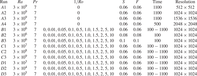
Class B runs consider three different values of  $S$ and $F$ in order to evaluate their impact on the flow statistics. We found that $S=F=0.06$ gave the optimum choice, as was also found in Bruneau et al. (Reference Bruneau, Fischer, Xiong and Kellay2018) for the non-rotating bubble DNS. Class C runs use the optimum grid resolution and values of $S,F$ found from runs A and B, but now with varying $Ro$ and $Ra$ in order to explore the role of rotation on the flow properties.
The results shown in the following sections correspond to the statistically stationary regime of the flow. In this regime, the ensemble average  $\langle \cdot \rangle$ is approximated using a time average, and an average over $\phi$, the latter being appropriate because the system is statistically invariant with respect to $\phi$. The statistics depend only on the latitudinal coordinate $\theta$, and owing to symmetry, we plot the results only over the range $\theta \in [0,{\rm \pi} /2]$.
3. Results and discussion: single-point information
We begin with a visual, qualitative comparison of the effects of  $Ro$ and $Ra$ on the instantaneous properties of the flow. In figure 1 we plot the temperature, TKE and enstrophy fields for $1/Ro=0$ and for $Ra=3\times 10^{6}$ and $Ra=3\times 10^{9}$ to see the effect of varying $Ra$. The same quantities are also plotted for $Ra=3\times 10^{9}$ at $1/Ro=10$ to see the effect of varying $Ro$. We note that the plumes and corresponding vortices in these visualisations are qualitatively very similar to those observed in experiments of a soap bubble (Meuel et al. Reference Meuel, Xiong, Fischer, Bruneau, Bessafi and Kellay2013, Reference Meuel, Coudert, Fischer, Bruneau and Kellay2018), and comparing the plumes for $Ra=3\times 10^{6}$ and $Ra=3\times 10^{9}$ in figure 1 we observe that the plumes become smaller and more convoluted in shape with increasing $Ra$. This is because of the enhanced turbulence intensity as $Ra$ is increased, leading to stronger mixing in the flow. Associated with this is that the thermal boundary-layer thickness reduces significantly in going from $Ra=3\times 10^{6}$ to $Ra=3\times 10^{9}$. Concerning the TKE and enstrophy, we find that as $Ra$ is increased, smaller-scale structures in the flow emerge, with strong enstrophy occurring at higher latitudes. For fixed $Ra$, as $1/Ro$ is increased the turbulent activity in the flow becomes restricted to lower latitudes where buoyancy is still strong enough to overcome the suppressing influence of the Coriolis force. The insets that highlight the thermal boundary layer indicate that the boundary layer and its thickness are only weakly affected by rotation. This is probably because of the fact that the Coriolis force is most active at the largest scales of the system, and plays a weaker role at the small scales of the flow, such as those that characterise the thin boundary layer at $Ra=3\times 10^{9}$.
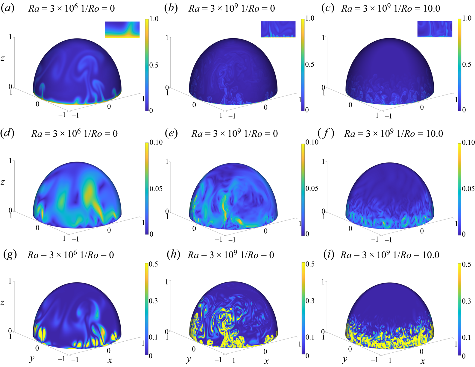
Figure 1. Instantaneous temperature (a–c), TKE (d–f) and enstrophy (g–i) for  $1/Ro=0$. Panels (a,d,g) show results for $Ra=3\times 10^{6}$, (b,e,h) show results for $Ra=3\times 10^{9}$ without rotation and (c,f,i) show results for $Ra=3\times 10^{9}$ and $1/Ro=10$. Insets to temperature visualisation highlight a section of the thermal boundary layer.
Note that in this work, the Rayleigh number ranges from  $Ra=3\times 10^{6}$ to $Ra=3\times 10^{9}$, which is much higher than the critical Rayleigh number for the flow. The critical Rayleigh number will depend on $1/Ro$, and our data indicates that for $1/Ro=10$, the critical Rayleigh number is larger than $Ra=3\times 10^{4}$ but smaller than $Ra=3\times 10^{5}$, while for $1/Ro=0$ it is between $Ra=3\times 10^{3}$ and $Ra=3\times 10^{4}$. A much larger set of DNS covering a wider portion of the parameter space would be required to determine the actual critical value and its dependence on $1/Ro$. This is left for future work.
3.1. The behaviour of the Reynolds and Nusselt numbers
We now turn to quantitatively analyse the statistics of the flow, beginning with an examination of the behaviour of the  $Re$ and $Nu$ in the flow. We remind the reader that based on their definitions, these are emergent properties of the flow, that depend upon the control variables $Ra, Ro$ and on the coordinate $\theta$.
In figure 2 the variation of  $Re$ for different $Ra$ and $1/Ro$ is shown. In each case, $Re$ reaches a maximum at some intermediate $\theta$, being small near the equator owing to the no-slip condition, and small near the north pole where buoyancy forces are weak because the heating is at the equator. The location of the maximum $Re$ is weakly affected by $Ra$ as well as $Ro$. The effect of $Ro$ on $Re$ is somewhat subtle, leading to an increase for some latitudes and a decrease for others. However, once $1/Ro\geq 1$ the suppression of turbulence at higher latitudes becomes evident. This suppression occurs because as $\theta$ increases, the buoyancy force decreases, and the Coriolis force becomes dominant. The Coriolis force does not generate TKE, and the Taylor–Proudman effect (combined with the fact that $\langle U_\theta \rangle =0$ for this flow) inhibits transport in the $\theta$ direction. As a result, TKE is not able to be transported to the top of the bubble. However, as $Ra$ is increased for fixed $Ro$, the convection becomes stronger and the Reynolds number increases at high latitudes.
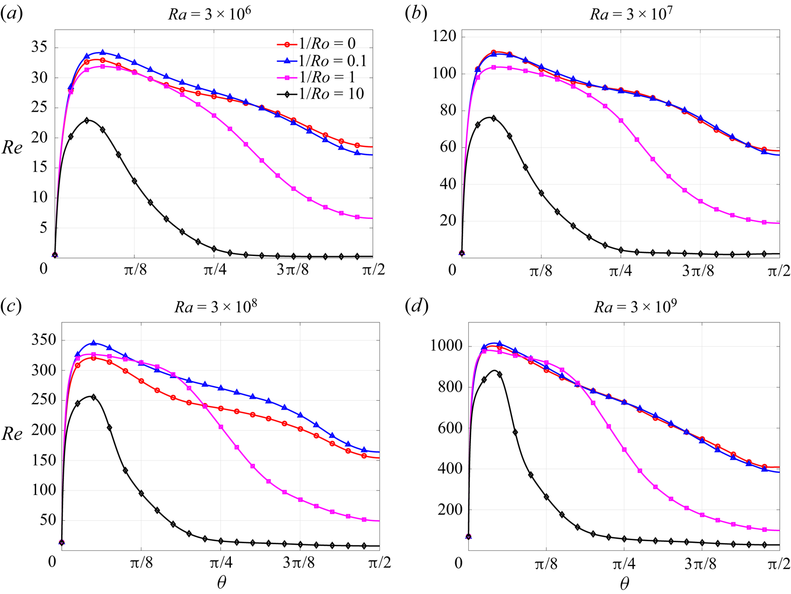
Figure 2. Variation of  $Re$ with $\theta$ for varying $1/Ro$ and $Ra$.
$Ra$.
In figure 3 we consider the total heat flux  $H_{T}(\theta )$ (defined in (2.10)) divided by its value on the equator $\theta =0$, in order to understand how the heat-transfer properties vary with $\theta$. The results reveal a weak dependence on $Ra$ but a strong dependence on $1/Ro$. In particular, as $1/Ro$ is increased, $H_T(\theta )/H_T(0)$ decays to zero more rapidly, owing to the turbulence being suppressed away from the equator by the Coriolis force, and the fact that buoyancy becomes weaker as $\theta$ increases. Again, the dependence of the Coriolis and buoyancy forces on $\theta$ makes the behaviour of the flow we are considering quite different from standard RRBC.

Figure 3. Variation of  $H_T(\theta )/H_T(0)$ with $\theta$ for varying $1/Ro$ and $Ra$.
$Ra$.
The scaling behaviour of  $Nu$ and $Re$ are shown in figure 4. The results for $Nu$ show that $Nu\sim Ra^{0.3}$, and the exponent seems to be independent on $1/Ro$. This value is not far from the classical theoretical prediction of $1/3$ for standard RBC (Ahlers et al. Reference Ahlers, Grossmann and Lohse2009). The results for $Re$ show that $Re\sim Ra^{0.49}$ for low $1/Ro$ and $Re\sim Ra^{0.53}$ for $1/Ro=10$. The insets reveal that for lower values of $Ra$,
$Ra$,  $Nu$ is slightly increased as $1/Ro$ is increased, while $Re$ decreases more significantly as $1/Ro$ is increased. However, as $Ra$ increases, this dependence on $1/Ro$ reduces because the buoyancy force becomes stronger relative to the Coriolis force as $Ra$ is increased, and hence the dependence on $1/Ro$ becomes weaker.

Figure 4. Scaling behaviour of  $Nu$ and $Re$ with $Ra$ for varying $1/Ro$. Insets highlight the influence of $1/Ro$.
3.2. The mean flows
In figure 5 we plot the normalised mean temperature  $\langle T\rangle /\delta T$, for different $Ra$ and $1/Ro$. When $1/Ro<1$, $\langle T\rangle /\delta T$ is weakly affected by rotation because the role of the Coriolis force is subleading in this regime. For $1/Ro\geq 1$, the Coriolis force and the associated Taylor–Proudman effect inhibits thermal transport at high latitudes, causing $\langle T\rangle /\delta T$ to reduce significantly as $1/Ro$ is increased. However, because in this regime heat transfer towards higher latitudes is significantly reduced, heat accumulates at lower latitudes. This explains the increase in $\langle T\rangle /\delta T$ that can be seen in figure 5 for $1/Ro\geq 1$ at lower latitudes. The thickness of the thermal boundary layer depends on $Ra$, which can be seen in figure 5, and scales as $\sim Ra^{-0.3}$, approximately independent of $Ro$. This is consistent with the scaling behaviour of $Nu$.
$Nu$.
Figure 5. The averaged temperature profiles  $\langle T\rangle$, normalised by $\delta T$, as a function of latitude, and for different $Ra, 1/Ro$.
In figure 6 we show results for  $\langle U_{\phi }\rangle$ normalised by $\sqrt {E_{turb}}$, for different $Ra$ and $1/Ro$. The results in figure 6 indicate that zonal-like mean flows are present, with the sign of $\langle U_{\phi }\rangle$ varying with $\theta$. Note that because $\langle U_{\theta }\rangle /\sqrt {E_{turb}}$ (not shown) is very small everywhere on the bubble, it is more appropriate to classify these as zonal flows, rather than LSC which are important in classical RBC. For the $1/Ro=0$ case, the symmetries of the problem would suggest that $\langle U_{\phi }\rangle =0$, which is not what we observe. This suggests that for the $1/Ro=0$ case, the finite mean velocity could be because of a lack of statistical convergence. We tried running the DNS for much longer for this case, but did not observe a reversal. This indicates that the zonal flow observed must fluctuate on very long timescales, somewhat analogous to the very long lifetimes of the LSC observed in classical RBC.

Figure 6. The mean longitudinal velocity  $\langle U_{\phi }\rangle$, normalised by $\sqrt {E_{turb}}$, as a function of latitude and for different $Ra, 1/Ro$.
As  $1/Ro$ is increased, the zonal flows associated with $\langle U_{\phi }\rangle$ become stronger, especially for larger $Ra$, with significant shear developing at lower latitudes. Unlike the no-rotation case, zonal flows may exist in the true steady state for finite $1/Ro$ because rotation provides the symmetry breaking factor required to allow $\langle U_{\phi }\rangle \neq 0$. The relation described by (2.14) describes how a mean temperature gradient $\partial _\theta \langle T\rangle$ could be associated with a mean shear $\partial _\theta \langle U_\phi \rangle$. However, given that $\partial _\theta \langle T\rangle \leq 0$, this effect cannot explain the non-monotonic variation of $\langle U_\phi \rangle$ observed in figure 6. An alternative mechanism for the generation of these zonal flows is via the Reynolds stresses associated with Rossby waves (Shukla & Stenflo Reference Shukla and Stenflo2003), which are possible on the bubble owing to the latitudinal variation of the Coriolis parameter. This is in contrast to RRBC where the Coriolis parameter is independent of position in the flow (i.e. there is no ‘beta-plane’ effect) so that Rossby waves cannot occur.
3.3. Temperature fluctuations
In figure 7 we plot the results for the root-mean-square (r.m.s.) fluctuating temperature  $\sqrt {\langle T'T'\rangle }$, normalised by $\delta T$, as a function of latitude and for different $Ra, 1/Ro$. For $1/Ro=0$, as $Ra$ is increased, the main effect is to simply shrink the thermal boundary layer, with the temperature fluctuations at high latitudes becoming weaker as $Ra$ is increased. As $1/Ro$ is increased, at higher latitudes the thermal fluctuations are significantly suppressed as the Coriolis force inhibits the transport of thermal fluctuations away from the boundary layer. However, in the vicinity of $\theta ={\rm \pi} /16$ (the precise region probably depends on $Ra$), we see that increasing $1/Ro$ actually increases the thermal fluctuations. This effect may be owing to something similar to Ekman suction wherein hot fluid is sucked out from the boundary layer owing to the transport produced by viscous and Coriolis forces on the fluid. For $1/Ro$, the enhancement in this region reduces with increasing $Ra$, however, it is possible that the enhancement would remain significant if $1/Ro$ were sufficiently large.

Figure 7. The r.m.s. fluctuating temperature  $\sqrt {\langle T'T'\rangle }$, normalised by $\delta T$, as a function of latitude and for different $Ra, 1/Ro$.
3.4. The Reynolds stress tensor and its anisotropy
We now turn to characterise the turbulence using the Reynolds stress tensor  $\boldsymbol {\sigma }\equiv \langle (\boldsymbol {U}-\langle \boldsymbol {U}\rangle )^{2}\rangle$ and for the bubble flow, the components of this tensor may be written in matrix form as
 \begin{equation} \boldsymbol{\sigma}=\begin{pmatrix} \langle U'_\theta U'_\theta\rangle & \langle U'_\phi U'_\theta\rangle \\ \langle U'_\phi U'_\theta\rangle & \langle U'_\phi U'_\phi\rangle \end{pmatrix}, \end{equation}
whose components we denote by  $\sigma _{ij}$, with $i,j$ either $\theta$ or $\phi$. We begin by considering the diagonal components of $\sigma _{\phi \phi }, \sigma _{\theta \theta }$ that contribute to the TKE, and the results are shown in figure 8. The results show strong anisotropy in the flow, with $\sigma _{\theta \theta }$ generally significantly larger than $\sigma _{\phi \phi }$, except at lower latitudes where $\sigma _{\phi \phi }$ is typically larger (the region of $\theta$ for which this occurs depends upon $1/Ro$). The buoyancy term in the Navier–Stokes equation makes a contribution $\boldsymbol {B}+\boldsymbol {B}^{\top }$ to the Reynolds stress equation, where $\boldsymbol {B}\equiv \beta g_\theta \boldsymbol {e_\theta }\langle T' \boldsymbol {U}'\rangle$, and in matrix form
 \begin{equation} \boldsymbol{B}+\boldsymbol{B}^{\top}=\beta g_\theta\begin{pmatrix} 2\langle T' U'_\theta \rangle & \langle T' U'_\phi\rangle \\ \langle T' U'_\phi\rangle & 0 \end{pmatrix}. \end{equation}
From this it is clear that buoyancy does not make a direct contribution to  $\sigma _{\phi \phi }$. Instead, buoyancy acts as a source for $\sigma _{\theta \theta }$, and some of this fluctuating energy is transferred to $\sigma _{\phi \phi }$ via redistribution mechanisms, such as the pressure-strain term (Pope Reference Pope2000). While this explains why $\sigma _{\theta \theta }$ is greater than $\sigma _{\phi \phi }$ over much of the domain, it is not consistent with the fact that $\sigma _{\phi \phi }$ is larger than $\sigma _{\theta \theta }$ for low latitudes. One way to understand this is that because the only finite contribution to $\boldsymbol {\nabla }\langle \boldsymbol {U}\rangle$ in the flow comes from the component involving $\partial _{\theta }\langle U_\phi \rangle$, then the transport equation for $\sigma _{\phi \phi }$ will involve a finite shear-production term, whereas $\sigma _{\theta \theta }$ does not, and the data for $\sigma _{\theta \phi }$ (below) indicate that this term is positive in the region where $\sigma _{\phi \phi }$ is larger than $\sigma _{\theta \theta }$ at lower latitudes.
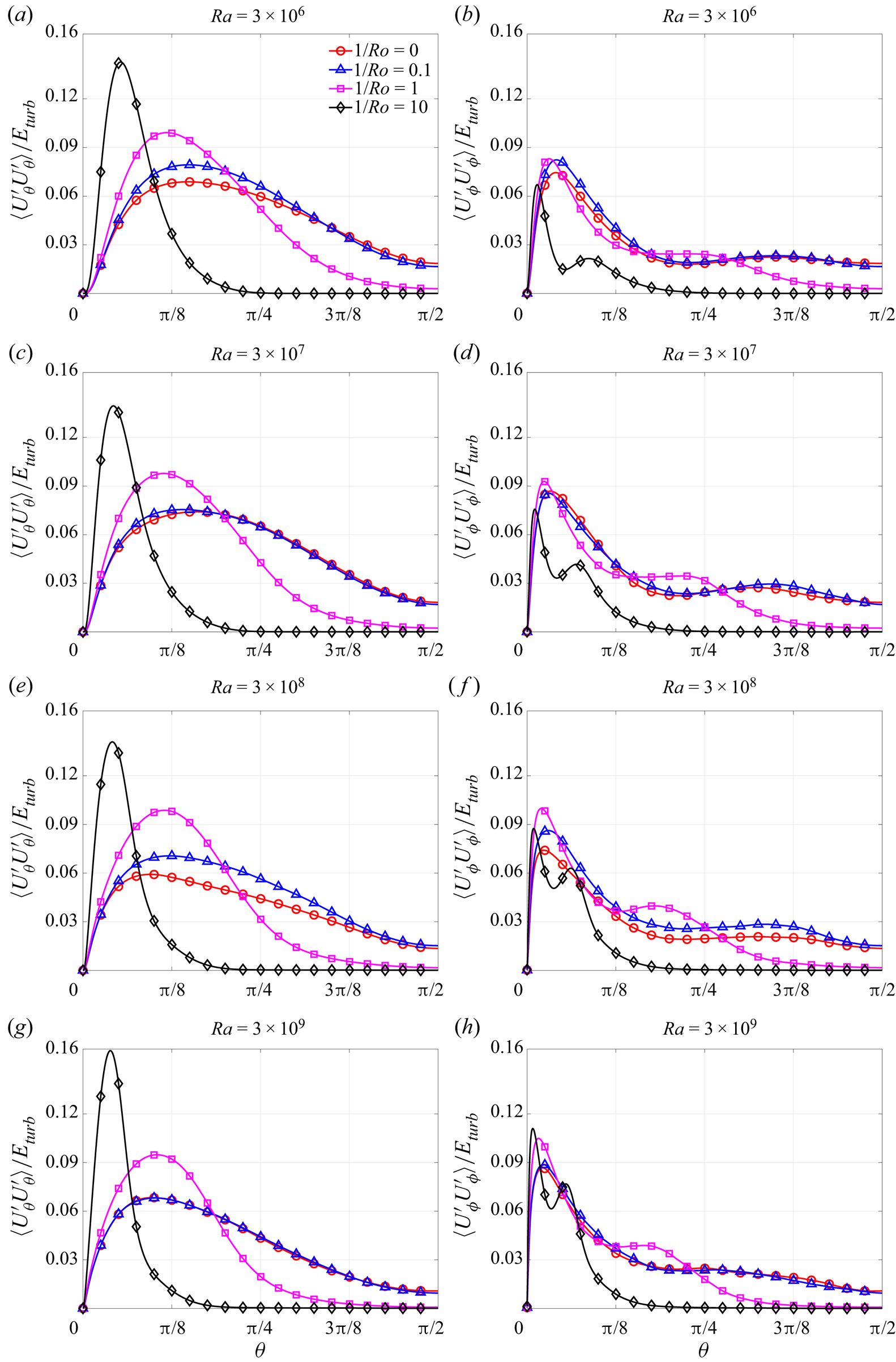
Figure 8. The diagonal Reynolds stress components  $\sigma _{\phi \phi }$ and $\sigma _{\theta \theta }$, normalised by $E_{turb}$, as a function of latitude and for different $Ra, 1/Ro$.
The Coriolis term also contributes to the redistribution of kinetic energy among the flow components. For example, the Coriolis acceleration projected along  $\boldsymbol {e_{\phi }}$ is
 \begin{equation} -2\boldsymbol{e_{\phi}}\boldsymbol{\cdot}(\boldsymbol{\varOmega}\times\boldsymbol{U})={-}2\varOmega U_{\theta}\boldsymbol{e_{\phi}}\boldsymbol{\cdot}(\boldsymbol{e_z}\times\boldsymbol{e_{\theta}}), \end{equation}
such that the flow in the latitudinal direction can produce an acceleration in the longitudinal direction, modifying the Reynolds stress associated with  $U'_\phi$. The net effect on both components is, however, zero because $(\boldsymbol {\varOmega }\times \boldsymbol {U})\boldsymbol {\cdot } \boldsymbol {U}=0$. Therefore, like the pressure–strain term, the Coriolis term produces a redistributive effect on the flow energy, only in this case, the effect arises from purely linear processes.
The results in figure 8 show oscillations in  $\sigma _{\phi \phi }$ as $\theta$ is increased, which are not present for $\sigma _{\theta \theta }$. These oscillations may be a result of the presence of LSC, whose influence on $\langle U_\phi \rangle$ was discussed earlier. As $1/Ro$ is increased, the effect on $\sigma _{\phi \phi }, \sigma _{\theta \theta }$ is non-monotonic, increasing or else decreasing their values for different $\theta$. As $\theta$ is increased, the buoyancy force tends to decrease, while the Coriolis term becomes dominant (see § 2). The Taylor–Proudman effect hinders the transport of fluctuations towards larger $\theta$, and because the Coriolis term does not produce TKE, this then implies that both $\sigma _{\theta \theta }$ and $\sigma _{\phi \phi }$ should decay as $\theta$ is increased. The results in figure 8 are consistent with this behaviour, and show that $\sigma _{\theta \theta }$ and $\sigma _{\phi \phi }$ reduce to almost zero for $\theta \geq {\rm \pi}/4$. We note that for $\theta \to 0$, the effect of rotation seems to vanish (which is also apparent for several of the other results). This is most probably owing to the fact that the Rossby number based on the boundary-layer thickness is $>O(1)$, i.e. the Coriolis force does not strongly affect the small scales of motion in the boundary layer.
The results for the shear-stress term  $\sigma _{\theta \phi }$, are shown in figure 9, and indicate that the maximum value of these stresses are an order of magnitude smaller than the diagonal Reynolds stresses. For the higher $Ra$ cases and for $1/Ro=0$, $\sigma _{\theta \phi }$ is positive near the equator, but becomes negative at higher latitudes. As $1/Ro$ is increased, this feature still persists; however, the location of the transition from positive to negative values, as well as the magnitudes of $\sigma _{\theta \phi }$, change significantly. The region of $\theta$ over which $\sigma _{\theta \phi }$ is finite decreases with increasing $1/Ro$ because in the regime $1/Ro\gg 1$, the Coriolis term suppresses $\sigma _{\theta \phi }$. In particular, while (3.3) implies that the Coriolis term can produce coupling between the components of $\boldsymbol {U}'$, the Coriolis term suppresses both components of $\boldsymbol {U}'$ so that (3.3) is also suppressed. Nearer to the equator this behaviour does not emerge because buoyancy forces are important there. As for the diagonal components of $\boldsymbol {\sigma }$, the dependence on $1/Ro$ is strongly non-monotonic, with the maximum value for $\sigma _{\theta \phi }$ on the bubble emerging for the $1/Ro=1$ case. However, the enhancement as $1/Ro$ is increased from zero to one is significantly stronger than for either $\sigma _{\theta \theta }$ or $\sigma _{\phi \phi }$.

Figure 9. The averaged Reynolds shear stress  $\sigma _{\phi \theta }$ along different latitudes of the soap bubble.
4. Results and discussion: scale-dependent information
Having explored the behaviour of the flow using one-point quantities that mainly characterise the large scales of the flow, we now turn to consider quantities that describe the properties of the flow at different scales. In this section we focus on the data for  $Ra=3\times 10^{9}$ for which there is the greatest scale separation in the flow, allowing us to most clearly explore the behaviour at dynamically distinct scales in the flow.
4.1. Kinetic energy and temperature spectra
For flows with strong buoyancy, there may exist a range of scales where buoyancy and inertial forces are both important, with viscous forces negligible. Assuming these forces balance, for stably stratified turbulence Bolgiano and Obukhov derived the well known Bolgiano–Obukhov (BO) scaling laws (Bolgiano Reference Bolgiano1959; Obukhov Reference Obukhov1959, hereafter BO59). In recent decades, there has been significant interest in exploring whether BO59 also applies in other flows such RBC (Lohse & Xia Reference Lohse and Xia2010) and Rayleigh–Taylor turbulence (Boffetta & Mazzino Reference Boffetta and Mazzino2017). Using BO scaling, then for two-dimensional turbulence with an inverse energy cascade. The following scaling is predicted (Boffetta & Mazzino Reference Boffetta and Mazzino2017):
 \begin{gather} E_U(k)\varpropto k^{{-}11/5}, \end{gather}
 \begin{gather}E_T(k)\varpropto k^{{-}7/5}, \end{gather}
where  $E_U(k)$ is the kinetic energy spectrum, and $E_T(k)$ is the thermal energy (half of the squared temperature).
The BO59 phenomenology is only expected to apply in regions of the flow sufficiently far from boundaries, and therefore will probably not apply at low latitudes in our flow. However, even for sufficiently high latitudes BO59 scaling may still not apply for at least two reasons. First, our flow takes place on a curved, not flat surface, and buoyancy in our flow is a function of latitude owing to the variation of  $\boldsymbol {g}\boldsymbol {\cdot }\boldsymbol {e}_\theta$ with $\theta$, as discussed earlier. However, one could argue that BO59 scaling might nevertheless hold in a local sense at scales small enough to be only weakly affected by the surface curvature and spatial variation of $\boldsymbol {g}\boldsymbol {\cdot }\boldsymbol {e}_\theta$. Second, our flow is affected by rotation, and at scales where $1/Ro_\ell >1$ BO59 will no longer apply owing to the role of the Coriolis force at these scales that is not included in BO59. The scaling that will emerge will then be determined by the relative roles of buoyancy, Coriolis forces and inertial forces in the flow at different length scales and different scalings may emerge in different scale ranges, where different forces in the flow balance. However, at scales where $1/Ro_\ell <1$, BO59 should still apply because at these scales the role of the Coriolis force is weak. In figure 10 we plot our results for $E_U(k)$ and $E_T(k)$. These are computed using spherical harmonic decompositions, with averaging over all $\theta ,\phi$ (see the Appendix for details).

Figure 10. Kinetic energy and thermal energy spectra for varying  $1/Ro$ and for $Ra=3\times 10^{9}$. Inset shows the compensated energy spectra.
Our results show that for  $1/Ro\leq 1$, a significant range of $kR$ exists over which the BO59 scaling accurately predicts the scaling behaviour of $E_U(k)$. For $1/Ro>1$, however, BO59 does not apply because the effect of rotation strongly affects the range of $kR$ where BO59 would otherwise emerge. The effect of rotation causes $E_U(k)$ to decay faster than $k^{-11/5}$ as $k$ increases. This may be understood by noting that if the Coriolis force dominated the behaviour of the spectrum, then the dynamically relevant parameter would be $\varOmega$ and the scaling that would emerge is $E_U(k)\propto k^{-3}$ (Smith & Waleffe Reference Smith and Waleffe1999).
In contrast, our results show that even for  $1/Ro=0$, BO59 does not accurately describe the scaling behaviour of $E_T(k)$ over any significant range of $kR$. In particular, $E_T(k)$ seems to decay more slowly than $E_T(k)\varpropto k^{-7/5}$ even for $1/Ro=0$. The most probable explanation for why BO59 does not describe $E_T(k)$ well, even though it does describe $E_U(k)$ well, is that unlike the velocity field, the temperature field is maximum at the equator and quickly reduces as $\theta$ is increased. Hence, because $E_T(k)$ is computed as an integral over the surface of the whole bubble, it will be strongly affected by the thermal boundary layer for which BO59 does not apply. Note that the steep temperature gradient near the equator behaves almost like a Heaviside function, and it is this which is responsible for the oscillations of $E_T(k)$ (Bruneau et al. Reference Bruneau, Fischer, Xiong and Kellay2018).
4.2. Spectral fluxes of kinetic energy, temperature and enstrophy
The behaviour of  $E_U(k)$ and $E_T(k)$ are determined by the behaviour of fluxes in spectral space that determine the energy and temperature fluctuations at different scales. In two-dimensional turbulence, in the absence of buoyancy, there are two inviscid integrals of motion, namely kinetic energy and enstrophy. According to standard arguments, at larger wavenumbers there is an upscale cascade of kinetic energy, and at smaller scales there is a downscale cascade of enstrophy. For our flow, where buoyancy and Coriolis forces also play a role, the behaviour of these cascades may differ, except at scales small enough for inertial forces to dominate over buoyancy and Coriolis forces.
In figure 11 we compute the kinetic energy flux  $\varPi _U(k)$, the enstrophy flux $\varPi _{\omega }(k)$ and thermal energy flux $\varPi _{T}(k)$, as a function of $kR$ (see the Appendix for details). The results indicate that except at the highest wavenumbers where $\varPi _U$ becomes slightly positive, $\varPi _U$ is predominantly negative, indicating an inverse energy flux driving kinetic energy to larger scales in the flow. However, the Reynolds number of our flow is too small to observe a cascade regime associated with a constant flux. Up until a certain value of $kR$, the magnitude of $\varPi _U$ reduces as $1/Ro$ is increases. This is simply understood in view of the fact that in the limit $1/Ro\to \infty$, the dynamical equations are linear and there is no energy transfer among scales. We also note, however, that above a critical $kR$ (which increases with increasing $1/Ro_\ell$), $\varPi _U$ converges to $\varPi _U$ for the non-rotating case $1/Ro=0$. This can be understood in terms of the scale-dependent Rossby number $Ro_\ell$ introduced in § 2, namely, that for any given rotation rate $\varOmega$ there is a scale below which $1/Ro_\ell <1$, indicating that the effects of rotation are subleading at these scales. As $\varOmega$ is increased, one has to go to a smaller scale before this regime is observed. The results in figure 11 are consistent with this, showing that $\varPi _U$ approaches the $1/Ro=0$ behaviour at larger $kR$ (i.e. smaller scale) as $1/Ro$ is increased.

Figure 11. The kinetic energy, enstrophy and thermal energy spectral fluxes.
The results for the enstrophy flux  $\varPi _{\omega }(k)$ as a function of wavenumber $k$, and for different $1/Ro$ are also shown in figure 11. As with two-dimensional turbulence on a flat surface, the results show that there is a downscale flux of enstrophy, but the Reynolds number of our flow is too small to observe a constant-flux cascade regime. As $1/Ro$ is increased, $\varPi _{\omega }(k)$ tends to be reduced, as the role of nonlinearity in the flow is reduced. However, we again observe that for sufficiently high $kR$, the effect of $1/Ro$ on $\varPi _{\omega }(k)$ disappears, corresponding to scales of the flow where $/Ro_\ell$. Overall, $\varPi _{\omega }(k)$ is much less sensitive to $1/Ro$ than $\varPi _U(k)$, which is because enstrophy is a predominantly small-scale quantity, whereas the velocity field is dominated (away from boundaries) by the large scales, for which the effect of rotation is the strongest.
The results for the thermal energy flux  $\varPi _{T}(k)$ shown in figure 11 show very weak sensitivity to $1/Ro$, except for $kR\lesssim 20$. This may seem surprising given that the temperature field, like the velocity field (but unlike the vorticity), is dominated (away from boundaries) by the largest scales of the flow, and therefore should be strongly susceptible to the effects of rotation. However, as noted earlier, the strongest contributions to the temperature field come from the thermal boundary layer, and the Rossby number based on the boundary-layer thickness is very small. This then explains the weak effect of $1/Ro$ on $\varPi _{T}(k)$.
In figure 12 we show the results for the buoyancy flux spectrum  $\varPi _{Buoy}$ which is of utmost importance because buoyancy is the mechanism generating the turbulent flow on the bubble. Indeed, $\varPi _{Buoy}>0$ for all $kR$, indicating that buoyancy injects TKE at all scales of the flow. The results for $1/Ro=0$ show that at the lowest $kR$,
$kR$,  $\varPi _{Buoy}$ decreases with increasing $kR$, which is in part associated with the fact that the velocity and temperature fluctuations are largest at the large scales. However, as $kR$ continues to increase, $\varPi _{Buoy}$ increases to a local maximum before vanishing for $kR\to \infty$ (owing to smoothness of the velocity and temperature fields). This indicates that there is a local, strong injection of TKE at the smaller scales in the flow. This must in fact be the case, because as already shown, the two-dimensional turbulent flow on the bubble exhibits an inverse kinetic-energy flux, and this requires an injection of TKE at smaller scales in the flow. Comparison with the results in figure 11 shows that the injection of TKE at small scales owing to buoyancy occurs at a smaller scale (larger $kR$) than that at which $\varPi _u$ becomes negative. Therefore, the inverse flux takes the TKE injected at small scales through $\varPi _{Buoy}$, and passes it to the larger scales in the flow, though not via a conservative cascade at these Reynolds numbers. The results in figure 12 show that as $1/Ro$ is increased, $\varPi _{Buoy}$ is suppressed except at the largest $kR$, where the effect of the Coriolis force is negligible. This then shows in scale-space, how rotation suppresses the mechanism of TKE injection into the flow, and thereby suppresses turbulence in the flow as $1/Ro$ is increased.

Figure 12. Buoyancy flux spectrum for varying  $1/Ro$ and for $Ra=3\times 10^{9}$.
4.3. Structure functions of temperature and velocity
Having considered the behaviour in Fourier space, we now consider the multiscale behaviour of the flow using structure functions. Not only does this provide insight in physical space, but it also allows us to consider the behaviour of fluctuations in the flow beyond the second-order information captured by the spectra.
The  $N$th order structure functions of $T$ and $\boldsymbol {U}$ are defined as
 \begin{gather} S^{{U}}_N\equiv\langle |[\boldsymbol{U}(\boldsymbol{x}+\boldsymbol{d},t) - \boldsymbol{U}(\boldsymbol{x},t)]\boldsymbol{\cdot} \boldsymbol{\hat{d}}|^{N} \rangle, \end{gather}
 \begin{gather}S^{T}_N\equiv\langle |T(\boldsymbol{x}+\boldsymbol{d},t) - T(\boldsymbol{x},t)|^{N} \rangle, \end{gather}
where  $\boldsymbol {\hat {d}}\equiv \boldsymbol {d}/\|\boldsymbol {d}\|$. Because the flow we are considering is homogeneous in $\phi$ but not in $\theta$, we choose $\boldsymbol {d}$ such that $\boldsymbol {d}\boldsymbol {\cdot } \boldsymbol {e}_\theta =0$, with $\|\boldsymbol {d}\|$ representing the linear (not geodesic) distance between two points on the sphere that have the same latitude.
For a two-dimensional turbulent flow, the BO59 scaling predictions are (Boffetta & Mazzino Reference Boffetta and Mazzino2017)
 \begin{gather} S^{{U}}_N\varpropto d^{3N/5}, \end{gather}
 \begin{gather}S^{T}_N \varpropto d^{N/5}. \end{gather}
For sufficiently small scales where molecular effects become important, the temperature and velocity fields are smooth and these scalings must give way to the alternative scaling  $S^{T}_N \propto S^{{U}}_N\propto d^{N}$ that may be demonstrated using a Taylor-series expansion.
One issue with computing the structure functions on the bubble is that the uniform grid used to solve the governing equations on the stereographic plane corresponds to a non-uniform grid on the curved bubble surface. This could then introduce a bias into the computation of the structure functions because only regions where the grid spacing is  $\geq d$ can contribute to the computation of the structure functions at scale $d$. Therefore, in order to compute the structure functions we used a high-order method to interpolate $\boldsymbol {U}$ and $T$ on to a grid that corresponds to points uniformly spaced on the surface of the bubble. Furthermore, in order to reduce statistical noise, we computed the structure functions by averaging over $\theta$, as well as over $\phi$ and time, which is consistent with how the spectral quantities were computed. One difference, however, is that for the structure functions we only average over the region $\theta \in [{\rm \pi} /18,{\rm \pi} /2]$ (unlike the earlier spectral results which had to be computed by averaging over all $\theta$ owing to the method of computation in terms of spherical harmonics). This is because close to the equator at $\theta =0$, the boundary layers, which are not accounted for in BO59, strongly influence the results (especially for the temperature). By only averaging over the region $\theta \in [{\rm \pi} /18,{\rm \pi} /2]$, the effect of these boundary layers on the computed structure functions is greatly reduced.
The results for  $S^{{U}}_N$ are shown in figure 13 for $N=1$ to $N=8$ and for different $1/Ro$. For $d/R\leq O(0.01)$, the smooth scaling $S^{{U}}_N\propto d^{N}$ emerges, but above this and for $1/Ro=0$, there is a clear range where BO59 seems to describe the behaviour well for each $N$ considered. This indicates the absence of intermittency in the velocity field, as is expected for two-dimensional turbulent flows Boffetta & Ecke (Reference Boffetta and Ecke2012), including those driven by buoyancy Boffetta & Mazzino (Reference Boffetta and Mazzino2017). As $1/Ro$ is increased, the BO59 scaling is still observed but over a region that becomes smaller as $1/Ro$ is increased. This is again simply owing to the fact that for fixed $Ra$, as $1/Ro$ is increased, the Coriolis force affects increasingly smaller scales in the flow, and BO59 does not apply to scales significantly affected by the Coriolis force. As $1/Ro$ is reduced, the values of $S^{{U}}_N$ at the larger scales decrease. This can be understood by noting that for sufficiently large $d/R$, $S^{{U}}_N$ is related to the Reynolds stress component $\sigma _{\phi \phi }$, and as shown in figure 8 and discussed earlier, this significantly reduces going from $1/Ro=0$ to $1/Ro=10$.

Figure 13. Velocity structure functions for  $Ra=3\times 10^{9}$ and for different $1/Ro$.
In figure 14 we show the results for  $S^{T}_N\propto d^{N}$. For $d/R\leq O(0.01)$, the smooth scaling $S^{{T}}_N\propto d^{N}$ emerges. Above this and for $1/Ro=0$, there is a clear range where BO59 seems to describe the behaviour well for smaller $N$, but significant departures are observed for larger $N$. While some of these deviations could be owing to the particularities of the rotating bubble flow we are considering, the study in Celani, Mazzino & Vozella (Reference Celani, Mazzino and Vozella2006) found similar behaviour in a non-rotating, two-dimensional Rayleigh–Taylor flow with flat geometry. Therefore, as was also concluded in Celani et al. (Reference Celani, Mazzino and Vozella2006), the deviations we observe from BO59 scaling for $S^{T}_N$ are most probably because of intermittency, something that is not captured in a mean-field theory like BO59. Note that the intermittency for the temperature field is much stronger than that for the velocity field. This is commonly observed in turbulent flows, and is usually explained in terms of the fact that the scalar equation (here temperature) does not have a pressure term, and it is the pressure term, via the incompressibility constraint, that hinders the growth of strong velocity gradients in the flow. Indeed, for this reason even a scalar field advected by a random Gaussian velocity field exhibits strong intermittency (Falkovich, Gawȩdzki & Vergassola Reference Falkovich, Gawedzki and Vergassola2001).

Figure 14. Temperature structure functions for  $Ra=3\times 10^{9}$ and for different $1/Ro$.
As  $1/Ro$ is increased, the behaviour remains the same, except that the range of $d/R$ over which BO59 is accurate for small $N$ reduces owing to the Coriolis force affecting the larger scales of the flow, which is not accounted for in BO59. For sufficiently large $1/Ro$, the Coriolis force would make a leading order contribution at all scales in the flow, and BO59 scaling would not be observed at any scale or for any $N$.
$N$.
5. Conclusions
We have used DNS to study the two-dimensional flow of a rotating, half soap bubble that is heated at its equator. This set-up replicates the experimental study of Meuel et al. (Reference Meuel, Coudert, Fischer, Bruneau and Kellay2018), but the DNS enables us to consider the flow in greater detail. The heating at the equator of the bubble produces buoyancy, while rotation generates a Coriolis forces in the fluid. However, owing to the curved surface of the bubble, the buoyancy and Coriolis forces vary with latitude on the bubble. This yields a flow that is strongly inhomogeneous and anisotropic, with rich flow behaviour.
We began by exploring the single-point properties of the flow, including the Reynolds  $Re$ and Nusselt $Nu$ numbers, mean fields and Reynolds stresses, all as a function of latitude. Increasing the Rayleigh number $Ra$ increases $Re$ and $Nu$, associated with an increasingly strong production of turbulence owing to convection in the flow. For a given $Ra$, we observe a non-monotonic dependence of the flow on the Rossby number $Ro$ for a range of different flow quantities. Moreover, the large-scale mean circulations that appear owing to convection are found to be strongly influenced by rotation, with the mean circulation becoming increasingly strong as $Ro$ decreases.
We then considered flow quantities that characterise the multiscale nature of the flow, including spectra and spectral fluxes of kinetic and thermal energy, enstrophy and structure functions of velocity and temperature. The fluxes show that just for non-buoyant two-dimensional turbulence on a flat surface, there is an upscale flux of kinetic energy at larger scales, and a downscale flux of enstrophy at smaller scales. The kinetic energy spectrum and velocity structure functions are well described by BO (BO59) scaling at scales where the effects of rotation are weak. The thermal energy spectrum and temperature structure functions are sensitive to contributions from the thermal boundary layer, where most of the thermal fluctuations are contained. Provided the temperature statistics are computed away from this boundary layer they are found to satisfy BO59 scaling quite well for low-order structure functions, but deviations are strong at higher orders owing to intermittency. This is unlike the velocity structure functions, which satisfy BO59 scaling at all orders owing to the absence of intermittency in the velocity field, associated with the inverse energy flux in the flow.
One interesting direction for future work would be to perform the DNS at much larger  $Ra$ for which the scale separation in the flow will be large. This will allow researchers to explore scales of the flow where, for example, Coriolis forces and buoyancy forces approximately balance or else Coriolis and inertial forces approximately balance (depending on the flow parameters) as well as scales much smaller than the buoyancy scale where the role of temperature fluctuations become dynamically passive and inertially dominated dynamical ranges may emerge.
Supplementary movies
Supplementary movies are available at https://doi.org/10.1017/jfm.2021.610.
Funding
This work was funded by the National Natural Science Foundation of China grant numbers 11872187 and 12072125. The authors thank SCTS/CGCL HPCC of HUST for providing computing resources and technical support. Y.L.X. acknowledges Cyclobulle Collaboration and the ANR grant for supporting his postdoctoral research opportunity at Institut de Mathématiques de Bordeaux from 2011 to 2013, which initialised the present study.
Declaration of interests
The authors report no conflict of interest.
Appendix A. Spherical harmonic decompositions
Let  $\varPsi$ be an arbitrary scalar field which can be expanded in a series of spherical harmonic functions
 \begin{equation} \varPsi(\theta,\phi)=\sum_{l=0}^{+\infty}\sum_{m={-}l}^{{+}l}\varPsi^{m}_{l}Y^{m}_{l}(\theta,\phi), \end{equation}
where  $Y^{m}_l$ is the spherical harmonic function, defined as
 \begin{equation} Y^{m}_l(\theta,\phi)=\sqrt{\frac{2l+1}{4{\rm \pi}}\frac{(l-m)!}{(l+m)!}}P^{m}_l(\cos(\theta))e^{im\phi}, \end{equation}
and  $P^{m}_l$ is the corresponding adjoint Legendre polynomial. The expansion coefficient of $\varPsi ^{m}_l$ can be calculated based on the orthogonality of the spherical harmonic functions, with the following formula:
 \begin{equation} \varPsi_l^{m}=\int^{2{\rm \pi}}_{0}\int^{{\rm \pi}/2}_{0}\varPsi(\theta,\phi)[Y_l^{m}(\theta,\phi)]^{*}\sin(\theta)\,\textrm{d}\theta \,\textrm{d}\phi, \end{equation}
where  $*$ denotes the complex conjugate. Note that the integral over $\phi$ in the preceding formula actually corresponds to calculating the Fourier transform, and we may write
 \begin{equation} \varPsi_l = \left(\sum^{{+}l}_{m={-}l}|\varPsi_l^{m}|^{2}\right)^{{1}/{2}}. \end{equation}
Using this, the power spectrum of the function  $\varPsi$ can be calculated as
 \begin{equation} |\varPsi|^{2} = \sum_{l=0}^{+\infty}\varPsi_l^{2} = \sum_{l=0}^{+\infty}\sum_{m={-}l}^{{+}l}|\varPsi_l^{m}|^{2}. \end{equation}
We refer to the square of the temperature as the thermal energy, whose power spectrum is calculated by
 \begin{equation} |T|^{2} =\sum^{+\infty}_{l=0}T_l^{2}=\sum^{+\infty}_{l=0}\sum^{l}_{m={-}l}|T_l^{m}|^{2}, \end{equation}
with
 \begin{equation} T^{m}_l =\int^{2{\rm \pi}}_{0}\int^{{\rm \pi}/2}_{0}T(\theta,\phi)(Y^{m}_l(\theta,\phi))^{*}\sin(\theta)\,\textrm{d}\theta \,\textrm{d}\phi. \end{equation}
Similar spherical harmonic decompositions may also be used to calculate the energy, enstrophy and thermal energy fluxes. The formula for calculating the energy flux is
 \begin{equation} \varPi_U(l') = \int_{l'}^{+\infty}\sum_{m={-}l}^{{+}l}\boldsymbol{I}_l^{m}\boldsymbol{\cdot}(\boldsymbol{U}_l^{m})^{*} \,\textrm{d}l, \end{equation}
where  $\boldsymbol {U}_l^{m}$ is the spherical harmonic decomposition coefficient of the velocity field
 \begin{equation} \boldsymbol{U}_l^{m} = \int^{2{\rm \pi}}_{0}\int^{{\rm \pi}/2}_{0}\boldsymbol{U}(Y^{m}_l(\theta,\phi))^{*}\sin(\theta)\,\textrm{d}\theta \,\textrm{d}\phi, \end{equation}
and  $\boldsymbol {I}_l^{m}$ is the coefficient obtained after spherical harmonic decomposition of the nonlinear term of the Navier–Stokes equation
 \begin{equation} \boldsymbol{I}_l^{m}=\int^{2{\rm \pi}}_{0}\int^{{\rm \pi}/2}_{0}(\boldsymbol{U}\boldsymbol{\cdot}\boldsymbol{\nabla})\boldsymbol{U}(Y^{m}_l(\theta,\phi))^{*}\sin(\theta)\,\textrm{d}\theta \,\textrm{d}\phi. \end{equation}
The flux of enstrophy can be obtained by
 \begin{equation} \varPi_\omega(l') = \int_{l'}^{+\infty}\sum_{m={-}l}^{{+}l}Z_l^{m}\cdot(\omega_l^{m})^{*} \,\textrm{d}l, \end{equation}
where
 \begin{equation} \omega_l^{m}=\int^{2{\rm \pi}}_{0}\int^{{\rm \pi}/2}_{0}\omega(Y^{m}_l(\theta,\phi))^{*}\sin(\theta)\,\textrm{d}\theta \,\textrm{d}\phi, \end{equation}
and
 \begin{equation} Z_l^{m}=\int^{2{\rm \pi}}_{0}\int^{{\rm \pi}/2}_{0}(\boldsymbol{U}\boldsymbol{\cdot}\boldsymbol{\nabla})\omega(Y^{m}_l(\theta,\phi))^{*}\sin(\theta)\,\textrm{d}\theta \,\textrm{d}\phi. \end{equation}
Finally, the thermal energy flux is
 \begin{equation} \varPi_T(l')=\int_{l'}^{+\infty}\sum_{m={-}l}^{{+}l}H_l^{m}(T^{m}_l)^{*} \,\textrm{d}l, \end{equation}
where
 \begin{equation} H_l^{m}=\int^{2{\rm \pi}}_{0}\int^{{\rm \pi}/2}_{0}(\boldsymbol{U}\boldsymbol{\cdot}\boldsymbol{\nabla})T(Y^{m}_l(\theta,\phi))^{*}\sin(\theta)\,\textrm{d}\theta \,\textrm{d}\phi. \end{equation}


 Open access