


1. Introduction
When a turbulent fluid flows over a flexible plate, the plate vibrates and radiates sound. Such fluid–structure–acoustic interaction arises in several marine and aerospace engineering applications. We study this interaction in the context of a canonical problem – one-way coupled structural vibration of, and sound radiated by, a rectangular elastic plate embedded in the bottom wall of a turbulent channel. By one-way coupled, we mean that the fluid affects the solid and not vice versa, and the solid affects the acoustic medium and not vice versa. Most previous studies (Hwang & Maidanik Reference Hwang and Maidanik1990; Hambric, Hwang & Bonness Reference Hambric, Hwang and Bonness2004; Esmailzadeh et al. Reference Esmailzadeh, Lakis, Thomas and Marcouiller2009; Blake Reference Blake2017) of plate vibration and far-field sound used wall-pressure models. Advances in high-performance computing now allow us to directly compute the unsteady turbulent wall-pressure fluctuations at moderate Reynolds numbers using direct numerical simulation (DNS) (Moin & Mahesh Reference Moin and Mahesh1998; Lee & Moser Reference Lee and Moser2015). We use these time-domain DNS wall-pressure fluctuations to study the plate vibration and far-field sound.
Recently, DNS has been used to investigate two-way coupled fluid–structure interaction of compliant walls in turbulent channels. Rosti & Brandt (Reference Rosti and Brandt2017) performed a DNS-based simulation of a hyper-elastic wall in turbulent channel flow. They examined the effect of elasticity and viscosity of the wall on the fluid–structure interaction, and found that skin friction increases with elasticity. Also, for low viscosity, the interface deformation is determined by the fluid fluctuations, while for high viscosity, the deformation is determined by the solid properties. Due to the wall compliance, they observe two distinct features: a sharp decrease in the velocity near the wall and an increase in the near-wall turbulence. Both these features are consistent with the experimental work of Wang, Koley & Katz (Reference Wang, Koley and Katz2020), where they study the advected modes of deformation and streamwise-aligned waves that travel in the spanwise direction. Esteghamatian, Katz & Zaki (Reference Esteghamatian, Katz and Zaki2022) studied the propagation of Rayleigh waves in a compliant wall. They found that similar advection velocity of near-wall pressure fluctuations and phase speed of Rayleigh waves lead to a local pressure minimum.
Previous studies of plate vibration (Hambric et al. Reference Hambric, Hwang and Bonness2004; De Rosa & Franco Reference De Rosa and Franco2008; Ciappi et al. Reference Ciappi, Magionesi, De Rosa and Franco2009; Esmailzadeh et al. Reference Esmailzadeh, Lakis, Thomas and Marcouiller2009; Ciappi et al. Reference Ciappi, Rosa, Franco, Guyader and Hambric2015; Hambric, Sung & Nefske Reference Hambric, Sung and Nefske2016; Blake Reference Blake2017) that use wall-pressure models rely on thin-plate theory (also called Poisson–Kirchoff plate theory) to describe the plate dynamics and modal summation to evaluate the plate response. Modal summation requires the plate's natural frequencies and natural mode shapes. For a plate described by thin-plate theory, analytical solutions can be derived for these frequencies and modes only when simply supported boundary conditions (BCs) are applied on any two opposite sides; see Reddy (Reference Reddy2006) for a discussion on this topic. Alternative BCs require numerical solutions using methods such as the finite element method and spectral methods. We describe the plate dynamics using three-dimensional elasticity theory, and use the finite element method along with direct time integration to compute the plate response. This approach works for both thin and thick plates, and is not limited by the number of modes used in the modal summation.
Some effects of the plate BCs on plate response have been identified by Hambric et al. (Reference Hambric, Hwang and Bonness2004) using the modified Corcos wall-pressure model. For frequencies where the plate streamwise modal wavenumber is much smaller than the wall-pressure convective wavenumber, they found that the streamwise wavenumbers that contribute the most to the modal forcing depend considerably on the plate BC. For a plate with a free edge, the wavenumbers around the wall-pressure convective wavenumber contribute the most, while for a plate with only simply supported and clamped edges, the wavenumbers around the plate streamwise modal wavenumber contribute the most. However, for frequencies where the plate streamwise modal wavenumber is close to or larger than the wall-pressure convective wavenumber, they found such dependence on BC to be absent. For these frequencies, irrespective of the BC, the wavenumbers around the wall-pressure convective wavenumber contribute the most to the forcing.
Scaling laws for the ratio of plate-averaged displacement power spectral density (PSD) to wall-pressure PSD have been proposed by Ciappi et al. (Reference Ciappi, Magionesi, De Rosa and Franco2012). Based on experimental measurements of different plate materials, plate thicknesses and turbulent flow velocities in both water and air, they proposed two scaling laws. One included the structural damping and the other did not.
Most previous theoretical studies that compute the far-field sound radiated due to turbulent flow-induced plate vibration use the method of stationary phase (e.g. Junger & Feit Reference Junger and Feit1986; Skelton & James Reference Skelton and James1997; Fahy & Gardonio Reference Fahy and Gardonio2007; Blake Reference Blake2017). Blake (Reference Blake2017) discusses several features of the far-field sound. A quantity important for the sound is the ratio of the acoustic wavenumber to the modal wavenumber along each direction. This ratio determines the plate region that effectively radiates sound after cancellation, for e.g. the plate surface, the plate edges and the plate corner. Further, the angular locations where each mode radiates the most depend on this ratio in addition to the mode order.
In this paper, we use the time-domain turbulent wall-pressure fluctuations extracted from a DNS of a turbulent channel to compute the plate vibration and radiated sound. The fluid–structure–acoustic coupling is assumed to be one-way coupled. The objective of this one-way coupled study is to perform a detailed analysis of each component involved in the interaction and provide results that can be used as a baseline for future two-way coupled studies to gauge the extent of interaction. We also discuss these one-way coupled results in the context of a fully coupled problem. The questions addressed in this paper are: (i) How does the effect of near-wall burst-sweep events on the plate vibration depend on the plate vibration time scale and plate BC? (ii) How do the plate vibration and sound radiation vary with the plate BCs, plate material and Reynolds numbers? (iii) What are the features of the plate displacement and acoustic pressure spectra over different frequency ranges? We consider a total of 12 different combinations of the problem parameters: three plate BCs (all sides clamped, all sides simply supported and three sides clamped with one side free), two plate materials (synthetic rubber and stainless steel) and two friction Reynolds numbers (180 and 400). To the best of our knowledge, this is the first such study to compute DNS-based vibroacoustic responses of elastic plates.
The rest of the paper is organized as follows. Section 2 describes the problem set-up. The simulation methodology is discussed in § 3, and the results are discussed in § 4. Section 4.1 shows the visualization of the fluid–structure–acoustic interaction. In § 4.2 we discuss the effect of plate vibration time scale on the plate behaviour away from the boundaries, and in § 4.3 we discuss the plate behaviour near boundaries. Section 4.4 discusses the features of the plate-averaged displacement spectrum. In § 4.5 we show the plate deformation patterns, and in § 4.6 we discuss the features of the acoustic pressure spectrum for the sound radiated by the plate vibration. The paper is summarized in § 5.
2. Problem definition
Throughout the paper,  $x$,
$x$,  $y$ and $z$ denote the streamwise, wall-normal and spanwise directions, respectively. The superscripts $f$,
$f$,  $s$ and $a$ denote fluid, solid and acoustic quantities, respectively. The fluid, solid and acoustic equations are non-dimensionalized using the density of the fluid, $\rho ^f$, the channel half-height, $\delta$, and the friction velocity, $u_{\tau }^f$. The friction velocity, $u^f_{\tau }$, is defined to be $\sqrt {\tau _w^f/\rho ^f}$, where $\tau _w^f$ is the mean wall shear of the turbulent flow.
2.1. Computational domain and boundary conditions
Figure 1 shows the computational domain used to simulate the problem. The blue, yellow and orange regions denote the fluid, solid and acoustic subdomains, respectively. The fluid subdomain is a channel of size  $L_x^f\times L_y^f\times L_z^f$, where $L_x^f = 6{\rm \pi} \delta$, $L_y^f = 2\delta$ and $L_z^f = 2{\rm \pi} \delta$. The solid subdomain is a plate of size $L_x^s\times L_y^s\times L_z^s$, where $L_x^s=(6{\rm \pi} /5)\delta$, the plate thickness $L_y^s=0.004\delta$ and $L_z^s= (2{\rm \pi} /5)\delta$. The acoustic subdomain is the entire bottom half-space below the plate.

Figure 1. Computational domain.
We choose the plate dimensions such that the streamwise plate length,  $L_x^s$, is sufficiently larger than the dominant wall-pressure wavelength. At $Re_\tau =180$ and $400$, $\lambda _x \approx 2\delta$ dominates the wall pressure (Anantharamu & Mahesh Reference Anantharamu and Mahesh2020), which is considerably lower than $L_x^s=(6{\rm \pi} /5)\delta$. In inner units, these wavelengths are $\lambda _xu_{\tau }^f/\nu ^f\approx 377$ and $838$ at $Re_\tau =180$ and $400$, respectively, while the plate lengths are $L_x^su_{\tau }^f/\nu ^f=679$ and $1508$ at $Re_\tau =180$ and $400$, respectively.
The large streamwise ( $L_x^f$) and spanwise ( $L_z^f$) extents of the channel are essential to include the contribution of large-scale turbulent structures to the wall-pressure fluctuations. The large extents also eliminate any spurious high levels that might otherwise be observed (Choi & Moin Reference Choi and Moin1990) in the wall-pressure wavenumber–frequency spectrum at low wavenumbers and frequencies. The arrow in figure 1 denotes the direction of the mean turbulent flow inside the channel. For better accuracy of high-frequency fluctuations, the fluid equations are solved in a moving frame of reference similar to Bernardini et al. (Reference Bernardini, Pirozzoli, Quadrio and Orlandi2013).
The plate is centred and baffled. The three plate BCs considered are: all four sides clamped ( $\mathrm {CCCC}$), three sides clamped and one side free (CCCF) and all four sides simply supported ( $\mathrm {SSSS}$). Here, the clamped BC ( $\mathrm {C}$) implies zero displacements in the $x$,
$x$,  $y$ and $z$ directions and the simply supported BC ( $\mathrm {S}$) implies zero displacements in the $y$ (wall-normal) direction, and free BC ( $\mathrm {F}$) implies no constraint on the displacements. Figure 2 shows a schematic of the different BCs and also the orientation of the edges. At the interface between the plate and acoustic medium, a Neumann BC is imposed on the acoustic pressure using the plate acceleration.

Figure 2. Plate BCs. Arrow denotes the direction of mean flow.
2.2. Simulation parameters
The fluid inside the channel is chosen to be incompressible air. Assuming room temperature, the fluid density  $\rho ^f$ is $1.225\ \textrm {kg}\ \textrm {m}^{-3}$ and the fluid kinematic viscosity $\nu ^f$ is $1.562\times 10^{-5}\ \textrm {m}^2\ \textrm {s}^{-1}$. The channel half-height, $\delta$, is chosen to be $1.25$ cm. The friction Reynolds numbers considered are $Re_{\tau }=180$ and $Re_{\tau }=400$, where $Re_{\tau }$ is defined to be $u^f_{\tau }\delta /\nu ^f$. To increase the Reynolds number, we increase the flow velocity while keeping the remaining parameters constant. This yields a friction velocity, $u_{\tau }^f$, of around $0.225\ \textrm {m}\ \textrm {s}^{-1}$ for $Re_{\tau }=180$ and around $0.5\ \textrm {m}\ \textrm {s}^{-1}$ for $Re_{\tau }=400$.
We consider two plate materials: synthetic rubber – a soft material; and stainless steel – a stiff material. The two materials are assumed to be elastic. For synthetic rubber, the density, Young's modulus and Poisson's ratio are set to  $1522\ \textrm {kg}\ \textrm {m}^{-3}$, $50 \textrm {MPa}$ and 0.4, respectively. For stainless steel, the density, Young's modulus and Poisson's ratio are set to $7500 \textrm {kg}\ \textrm {m}^{-3}$, $180\ \textrm {GPa}$ and 0.305, respectively. For structural damping, we use the Rayleigh damping model. The stiffness-proportional damping coefficient is set to zero and the mass-proportional damping coefficient is computed such that the loss factor is $0.05$ at the first natural frequency of the plate. We set the maximum structural loss factor (at the first natural frequency) equal to 0.05 because most structures have a loss factor less than or equal to 0.05, and here the loss factor decreases with the natural frequency. It also ensures that the displacement levels are low enough to allow one-way coupled analysis. The acoustic medium is assumed to be air. Assuming room temperature, the speed of sound is then $343\ \textrm {m}\ \textrm {s}^{-1}$. Table 1 shows the resulting non-dimensional problem parameters for each case. In total, we have 12 cases – two Reynolds numbers, two plate materials and three plate BCs.
Table 1. Non-dimensional simulation parameters.

For the considered Reynolds numbers, a soft plate material such as synthetic rubber allows a multimodal vibroacoustic response. For a multimodal response, the first natural plate frequency  $(\omega _1)$ needs to be very small compared with the high-frequency turbulent motion set by $\nu ^f$ and $u_\tau ^f$, i.e. $\omega _1\nu ^f/{u_\tau ^f}^2$ should be much smaller than one. For the synthetic rubber plates, $\omega _1\nu ^f/{u_\tau ^f}^2$ is of order $0.1$, while for the stainless steel plates, $\omega _1\nu ^f/{u_\tau ^f}^2$ is of order $1$. Table 1 shows the first natural frequencies in inner units.
The wavelength of the acoustic radiation is much larger than the channel dimension and viscous length scales. The acoustic radiation wavelength is given as  $\lambda ^a = 2{\rm \pi} c^a/\omega$, where $\lambda ^a$ is the acoustic wavelength, $c^a$ is the speed of sound in the acoustic medium and $\omega$ is the dominant angular frequency. For the problem under investigation, the first mode of plate vibration dominates the acoustic response. Therefore, the acoustic radiation wavelength relative to the viscous length scale, $\nu ^f/u_\tau ^f$, can be estimated as $\lambda ^a/(\nu ^f/{u_\tau ^f}) = 2{\rm \pi} ({c^a/u_\tau ^f}/{\omega _1\nu ^f/{u_\tau ^f}^2})$, where $\omega _1$ is the first natural frequency of the plate vibration. Using the values of $c^a/u_\tau ^f$ and ${\omega _1\nu ^f/{u_\tau ^f}^2}$ provided in table 1, we can compute the value of $\lambda ^a/(\nu ^f/{u_\tau ^f})={\lambda ^a}^+$. Further, we compute the acoustic wavelength relative to the channel dimension, $\delta$, as $\lambda ^a/\delta = {\lambda ^a}^+/Re_\tau$. These ratios are given in table 2. Amongst all cases, the minimum and maximum values of $\lambda ^a/(\nu ^f/{u_\tau ^f})$ are $4\times 10^3$ and $5.39\times 10^5$, respectively, and the minimum and maximum values of $\lambda ^a/\delta$ are $25$ and $1365$, respectively. As $\lambda ^a/\delta \gg 1$ and $\lambda ^a/(\nu ^f/{u_\tau ^f})\gg 1$, the acoustic radiation might not alter the flow.
Table 2. Relevant acoustic parameters. Here  $k^a$, $k_p^{(1)}$ $\lambda ^a$ are the acoustic radiation wavenumber, plate wavenumber and acoustic radiation wavelength corresponding to the first plate vibration mode.

To analyse the acoustic radiation patterns, we can use past works where a simply supported plate is mostly considered as its analytical mode shapes and modal wavenumbers are known. For other BCs, these quantities are more involved. Therefore, to analyse the acoustic radiation patterns using conclusions from past literature, we define the plate wavenumber for the  $N$th mode as
 \begin{equation} k_p^{(N)}=\sqrt{\left(\frac{m{\rm \pi}}{L_x^s}\right)^2+ \left(\frac{n{\rm \pi}}{L_z^s}\right)^2}, \end{equation}
where  $m$ and $n$ are the mode orders of the $N$th mode in $x$ and $z$ directions, respectively. This definition is consistent with the panel wavenumber of Wallace (Reference Wallace1972), and for simply supported plates, the plate wavenumber is the modal wavenumber. The acoustic-to-plate wavenumber ratios corresponding to the first plate mode ( $N=1, m=1, n=1$) are given in table 2. Amongst all cases, the minimum and maximum values of the ratio are 0.0018 and 0.0967, respectively.
3. Simulation methodology
For both Reynolds numbers, we first simulate the turbulent flow until the flow becomes statistically stationary. The wall-pressure fluctuations are then stored for a total time of  $30\delta /u_{\tau }^f$ for $Re_{\tau }=180$ and $23\delta /u_{\tau }^f$ for $Re_{\tau }=400$. These fluctuations are converted to a stationary frame, and then used to compute the plate response for each Reynolds number, plate material and plate BC. The far-field sound is computed from the plate response. We discard the initial $15\delta /u_{\tau }^f$ units of the simulated response and sound for $Re_{\tau }=180$ cases and $8\delta /u_{\tau }^f$ units for $Re_{\tau }=400$ cases because they predominantly contain the plate's transient response. The remaining data are used to compute the statistics of the plate displacement and sound. Sections 3.1–3.3 describe the simulation methodologies for the fluid, solid and acoustic subproblems, respectively.
3.1. Fluid subproblem
To simulate the turbulent flow inside the channel, we solve the incompressible Navier–Stokes equations using DNS. The equations are
 \begin{equation} \left.\begin{array}{c@{}}
\displaystyle \dfrac{\partial u_i^f}{\partial
t}+\dfrac{\partial u_i^f u_j^f}{\partial x_j}
={-}\dfrac{1}{\rho^f}\dfrac{\partial p^f}{\partial x_i} +
\nu_f \dfrac{\partial^2 u_i^f}{\partial x_j \partial
x_j} \quad \textrm{and}\\ \displaystyle
\dfrac{\partial u_i^f}{\partial x_i} = 0.
\end{array}\right\} \end{equation}
\begin{equation} \left.\begin{array}{c@{}}
\displaystyle \dfrac{\partial u_i^f}{\partial
t}+\dfrac{\partial u_i^f u_j^f}{\partial x_j}
={-}\dfrac{1}{\rho^f}\dfrac{\partial p^f}{\partial x_i} +
\nu_f \dfrac{\partial^2 u_i^f}{\partial x_j \partial
x_j} \quad \textrm{and}\\ \displaystyle
\dfrac{\partial u_i^f}{\partial x_i} = 0.
\end{array}\right\} \end{equation}
Here,  $u_i^f$ is the fluid velocity, $p^f$ is the fluid pressure, $\rho ^f$ is the fluid density and $\nu ^f$ is the fluid kinematic viscosity. These equations are solved in a moving frame of reference using the collocated finite volume method of Mahesh, Constantinescu & Moin (Reference Mahesh, Constantinescu and Moin2004). This method is second-order-accurate in both space and time, and conserves kinetic energy discretely in the inviscid limit. The discrete kinetic energy conservation property reduces aliasing errors (Blaisdell, Spyropoulos & Qin Reference Blaisdell, Spyropoulos and Qin1996). The velocity of the moving frame is set to $(U_b,0,0)$, where $U_b$ is the bulk velocity of the turbulent flow. For friction Reynolds numbers $180$ and $400$, the velocity $U_b$ is set to $15.8u_{\tau }^f$ and $17.8u_{\tau }^f$, respectively. The moving frame of reference reduces the magnitude of the dispersive errors (Bernardini et al. Reference Bernardini, Pirozzoli, Quadrio and Orlandi2013) leading to better transfer of energy to small scales, and, therefore, better prediction of the high-frequency spectrum. The DNS is performed using our in-house flow solver, MPCUGLES.
The mesh used for the DNS is Cartesian. The control volumes are uniform in streamwise and spanwise directions, and are non-uniform with a hyperbolic tangent stretching in the wall-normal direction. Table 3 shows the number of control volumes in each direction, and the mesh resolution. The resolution is fine enough to resolve the small-scale, coherent fluctuations near the wall. The non-dimensional time step,  $\Delta t^f (u_{\tau}^f/\delta )$, used for the DNS is $5\times 10^{-4}$. The DNS has been validated. For figures comparing mean velocity, mean pressure and the root mean square (r.m.s.) and spectra of velocity and pressure fluctuations with the reference DNS of Moser, Kim & Mansour (Reference Moser, Kim and Mansour1999), we refer the reader to Appendix C of Anantharamu & Mahesh (Reference Anantharamu and Mahesh2020). The DNS-based wall-pressure statistics above $\omega \nu ^f/u_{\tau }^{\kern1.5pt f^2}\approx 2$ are likely not resolved. Therefore, to avoid any undepredictions of the statistics above this frequency, throughout the paper, we only consider the statistics below $\omega \nu ^f/u_{\tau }^{\kern1.5pt f^2}\approx 2$.
Table 3. Fluid mesh details.

3.2. Solid subproblem
To simulate the plate response, we solve the three-dimensional dynamic linear elasticity equations:
 \begin{equation} \rho^s \frac{\partial^2 d_i^s}{\partial t^2} = \frac{\partial \sigma^s_{ij}}{\partial x_j}, \end{equation}
using the continuous Galerkin finite element method. Here,  $\rho ^s$ is the solid density, $d_i^s$ is the solid displacement and $\sigma ^s_{ij}$ is the linear Cauchy stress tensor of the solid. For spatial discretization, we use the 27-node hexahedral element, and for temporal discretization, we use the trapezoidal rule. Our method is spatially third-order-accurate for the displacements, spatially second-order-accurate for the stresses and temporally second-order-accurate. These simulations are performed using our in-house solid solver, MPCUGLES-SOLID. For further solver details, we refer the reader to Anantharamu & Mahesh (Reference Anantharamu and Mahesh2021).
The plate mesh is Cartesian, and matches the fluid mesh at the fluid–solid interface. Since the two meshes match at the interface, we do not require any special strategy to transfer the wall-pressure fluctuations from the fluid mesh to the solid mesh. Note that the fluid wall-pressure fluctuations are converted from moving to stationary frame via Fourier interpolation before transferring them to the solid mesh. Table 4 shows the number of elements and resolution of the solid mesh. All solid simulations use a non-dimensional time step,  $\Delta t^s (u_{\tau }^f/\delta )$, of $5\times 10^{-4}$, which is same as that of the fluid DNS.
Table 4. Solid mesh details.

Table 5 shows the first 20 natural frequencies for each case in outer units. For validation of our in-house solid solver for static, dynamic and eigenvalue plate problems, we refer the reader to Appendix B of Anantharamu & Mahesh (Reference Anantharamu and Mahesh2021).
Table 5. First 20 natural frequencies for all the cases, non-dimensionalized with outer flow variables ( $\omega _j\delta /u_\tau$).

3.3. Acoustic subproblem
To simulate the sound radiated by the plate vibration, we solve the acoustic wave equation:
 \begin{equation} \frac{\partial^2p^a}{\partial t^2}-c^{a^2}\nabla^2p^a=0, \end{equation}
using the Green's function methodology. Here,  $p^a$ is the acoustic pressure and $c^a$ is the sound speed of the acoustic medium.
Since the plate is planar and baffled, we use the half-space Green's function of a baffled plate (Blake Reference Blake2017). This Green's function requires evaluating an integral over the plate and acoustic medium interface. To evaluate this integral, the interface is discretized into a surface mesh composed of nine-node quadrilateral surface elements. This surface mesh coincides with the plate's three-dimensional mesh, and therefore transferring the nodal acceleration from the plate mesh to this surface mesh is straightforward. This strategy yields the following expression for the acoustic pressure,  $p^a(\boldsymbol {x},t)$, at point $\boldsymbol {x}$ in the acoustic domain and time $t$:
$t$:
 \begin{align} p^a(\boldsymbol{x},t)=\frac{\rho^a}{2{\rm \pi}}\sum_{\substack{{e\in} \\ \textrm{surface} \\ \textrm{elements}}}\int_{\varGamma_e} \frac{1}{\|\boldsymbol{x}-\boldsymbol{y}\|_2}\left[\sum_{\substack{j \in \\ \textit{e}\textrm{th\ surface} \\ \textrm{element's} \\ \textrm{nodes}}} \boldsymbol{\tilde{a}}_j^s\left(t-\frac{\|\boldsymbol{x}- \boldsymbol{y}\|_2}{c^a}\right)\varphi_j(\,\boldsymbol{y})\right]\boldsymbol{\cdot} \boldsymbol{n}(\,\boldsymbol{y})\,\mathrm{d}\boldsymbol{y}. \end{align}
Here,  $\rho ^a$ is the acoustic medium density, $\sum _{\substack {{e}\in \\ \textrm {surface} \\ \textrm {elements}}}$ is the summation over all surface elements, $\varGamma _e$ is the $e$th surface element, $\|\boldsymbol {x}-\boldsymbol {y}\|_2$ denotes the $\ell _2$ norm of vector $\boldsymbol {x}-\boldsymbol {y}$, $\sum _{\substack {{j}\in \\ e\mathrm {{th}\ surface} \\ \textrm {element's} \\ \textrm {nodes}}}$ denotes summation over nodes of the $e$th surface element, $\boldsymbol {\tilde {a}}_j^s$ is the piecewise linear interpolant in time of the plate acceleration at the $j$th node, $\varphi _j$ is the shape function of the $j$th node of the surface element and $\boldsymbol {n}$ is the vector normal to the plate surface and pointing into the acoustic domain. We use two Gauss quadrature points in each direction to compute the element integral.
Note that the above wave equation is applicable only for a quiescent medium in the absence of any ambient mean flow or shear effects. The effect of the ambient mean flow on our acoustic results will depend on the ambient flow velocity scales relative to the speed of sound. If the velocity scales are comparable to the speed of sound, the acoustic waves might undergo refraction and reflection due to the velocity gradients. As a result, the ambient flow might alter the directivity patterns observed in the quiescent medium because refraction would bend the acoustic waves. However, if the velocity scales are significantly smaller than the speed of sound, the ambient flow might not have much effect on the acoustic radiation in the quiescent medium.
The sound pressure is computed at discrete points on a polar grid in the acoustic domain, and at discrete time instants. These points are  $(r_i\cos (\theta _j),r_i\sin (\theta _j),{\rm \pi} )$, where $r_i=r_o+i\Delta r; \theta _j=\theta _o+j\Delta \theta ; r_o=10{\rm \pi} ; \theta _o={\rm \pi} ; \Delta r=160{\rm \pi} /N_r; \Delta \theta ={\rm \pi} /N_{\theta };\,i=1,\ldots,N_r,\textrm { and }$ $j=1,\ldots,N_{\theta }$. Here, $N_r$ and $N_{\theta }$ are the number of points along radial and angular directions, respectively. Parameter $N_r$ is set to $15$ and $N_{\theta }$ is set to $19$. The time instants are uniformly separated by a non-dimensional time step of $\Delta t^a u_{\tau }^f/\delta$ equal to $5\times 10^{-4}$, which is the same as the fluid and solid simulation time step.
To validate the acoustic solver, we compute the sound radiated by a plate undergoing a spatially uniform cosine acceleration. For this problem, the analytical solution is
 \begin{equation} p^a(\boldsymbol{x},t) = \frac{\rho^a}{2{\rm \pi}}\int_\varGamma \frac{1}{\|\boldsymbol{x}-\boldsymbol{y}\|_2}\cos \left(\frac{2{\rm \pi}}{T}\left(t-\frac{\|\boldsymbol{x}- \boldsymbol{y}\|_2}{c^a}\right)\right)\,{\rm d} \boldsymbol{y}. \end{equation}
Here,  $T$ is the time period of the plate acceleration. We set the plate dimension to $6{\rm \pi} /5\times 2{\rm \pi} /5\times 0.004$, $c^a$ to $343$, $T$ to $1$, and compute the sound at the far-field point $\boldsymbol {x}=(0,0,-100{\rm \pi} )$ for time instants separated by a $\mathrm {d}t$ of $1/32$.
Figure 3 compares the acoustic pressure,  $p^a$, computed from our solver with the analytical solution as a function of time. Good agreement is observed.

Figure 3. Comparison of the analytical and numerical acoustic pressure at  $r=100{\rm \pi}$ below the plate centre. Solid line (blue), analytical solution; $\circ$ (red), numerical solution obtained using the acoustic solver.
4. Results
4.1. Visualization of the one-way coupled fluid–structure–acoustic interaction
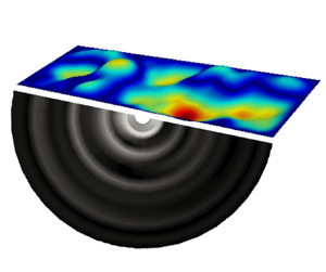
Figure 4 shows a synchronized visualization of the turbulent wall pressure exerted on the plate, plate displacement in the  $y$ direction and the sound radiated due to the plate vibration. We show three cases: $Re_\tau =400$; CCCC, CCCF, SSSS; synthetic rubber. Figure 4(a) shows the subdomain wall pressure at $Re_\tau =400$. The synthetic rubber plate deformations for CCCC, CCCF and SSSS BCs are shown in figures 4(b), 4(c) and 4(d), respectively, and the sound radiated for CCCC, CCCF and SSSS BCs is shown in figures 4(e), 4(f) and 4(g), respectively.

Figure 4. Synchronized instantaneous visualization of the turbulent wall pressure exerted on the plate at  $Re_\tau =400$, synthetic rubber plate deformation (displacement in $y$ direction) and the sound radiated due to the synthetic rubber plate vibration, in outer units. The flow direction is from left to right. (a) Wall pressure; (b–d) plate deformation for CCCC, CCCF, SSSS BCs; (e–g) sound radiated for CCCC, CCCF, SSSS BCs. In (b–d) the grid deformations are scaled up by a factor of 20.
The plate deformations are inhomogeneous, and this inhomogeneity varies with plate BCs. The deformation also has a range of length scales, of which a few are comparable with the turbulent wall-pressure length scales. However, the largest deformation length scales are considerably higher than the largest wall-pressure length scales. For all plate BCs, the crests and troughs of the plate deformation are mainly aligned in the streamwise direction and do not resemble plate mode shapes. The sound radiated due to these plate vibrations is nearly the same for all angular positions at a given radial distance, i.e. the plate acts like a monopole source of sound for all BCs. The directivity resembles that of a monopole source because the first plate mode contributes the most to the acoustic pressure, and the ratio of acoustic to plate wavenumber is very small for the first mode (0.0018–0.0036, given in table 2).
4.2. Effect of plate vibration time scale on the plate behaviour away from the boundaries
The turbulent wall-pressure signal consists of intermittent large-amplitude fluctuations and from previous works (Kim Reference Kim1989; Snarski & Lueptow Reference Snarski and Lueptow1995) we know that these fluctuations are the footprints of the burst-sweep cycle of events in the wall region. Specifically, the positive and negative peak events are produced by the near-wall local flow acceleration and deceleration events, respectively (Snarski & Lueptow Reference Snarski and Lueptow1995). Figure 5(a) shows the time history of turbulent wall pressure at the plate centre for  $Re_\tau =400$. The intermittent large-amplitude events are evident in the wall-pressure signal, with the negative peak events occurring more frequently than the positive peak events. This observation is consistent with that of Snarski & Lueptow (Reference Snarski and Lueptow1995).

Figure 5. Wall-pressure (a) and plate displacement (b,c) time history at the plate centre for  $Re_\tau =400$. (b) Synthetic rubber plate with CCCC BC. (c) Stainless steel plate with CCCC BC.
The time scale of plate vibration and the eddies in the inner region of the channel are similar for stainless steel plates and significantly different for synthetic rubber plates. The first natural frequency of these plates in inner units,  $\omega _1\nu ^f/u_{\tau }^{\kern1.5pt f^2}$ (given in table 1), is the ratio of the time scale of plate vibration and the eddies in the wall region. For stainless steel plates (referred to as ‘stiff plates’), $\omega _1\nu ^f/u_{\tau }^{\kern1.5pt f^2}$ is of order $1$, while for synthetic rubber plates (referred to as ‘soft plates’), $\omega _1\nu ^f/u_{\tau }^{\kern1.5pt f^2}$ is of order $0.1$, i.e. the soft plate vibration time scale is very small compared with the time scale of the near-wall eddies. Figures 5(b) and 5(c) show the displacement of synthetic rubber and stainless steel plate centres, respectively, for CCCC BC, at $Re_\tau =400$.
For soft plates ( $\omega _1\nu ^f/u_{\tau }^{\kern1.5pt f^2} \ll 1$), the displacement signal away from the boundaries resembles an amplitude-modulated (AM) wave and does not consist of intermittent large-amplitude events. However, for stiff plates ( $\omega _1\nu ^f/u_{\tau }^{\kern1.5pt f^2} \sim 1$), the displacement signal does not resemble an AM wave and shows intermittent large-amplitude events, similar to the wall pressure. This is because the soft plate undergoes strong multimodal excitation, and the stiff plate experiences weak modal excitation. The stronger the modal excitation, the lesser the similarities between the wall-pressure and plate displacement signals. Here, the modal excitation is considered to be strong when it has a significant contribution to the plate vibration energy and weak when this contribution is less. The two distinct features of an AM wave are (i) rapid oscillations characterized by a carrier frequency and (ii) relatively slowly varying amplitude marked by an envelope.
The envelope of an AM signal may be obtained using the Hilbert transform:
 \begin{equation} \mathcal{H}(t) = \mathcal{H}\{x(t)\} = \frac{1}{\rm \pi}P\int_{-\infty}^{+\infty}\frac{x(\tau)}{t-\tau}\, {\rm d}\tau, \end{equation}
where  $P$ is the Cauchy principal value of the integral and $\tau$ is the time shift. The envelope, $E(t)$, of signal $x(t)$ is given by
 \begin{equation} E(t) = E\{x(t)\} = \sqrt{x^2(t)+\mathcal{H}^2(t)}. \end{equation}
Figure 6(a,b) shows plate deformation time history of the plate centre and the envelope for CCCC at  $Re_\tau =400$. For the soft plate, the rapid oscillations have a single carrier frequency, which is the first plate natural frequency, and the envelope is similar to that of an over-modulated wave. In contrast to the soft plate, the rapid oscillations of the stiff plate consist of a range of frequencies, and no distinct slowly varying envelope is observed.

Figure 6. Displacement time history of the (a) synthetic rubber and (b) stainless steel plate centre for CCCC BC at  $Re_\tau =400$, in outer units. Black line, displacement; red line, envelope of the displacement ( $E(t)$ and $-E(t)$).
The amplitude-modulation spectrum (Fourier coefficients of displacement signal,  $\hat {d}(\omega )$) of the soft plate consists of a single carrier frequency, $\omega _c$, where $\hat {d}(\omega _c)={max}\{\hat {d}(\omega )\}$, and asymmetric sidebands with the upper sideband ( $\omega >\omega _c$) having more energy than the lower sideband ( $\omega <\omega _c$). Figures 7(a) and 7(b) show the AM spectrum of synthetic rubber and stainless steel plate displacement time history, respectively. For an AM wave, the spectrum is expected to have a carrier component and sidebands. For the soft plate (figure 7a), the spectrum peaks at the plate first natural frequency, i.e. $\omega _c=\omega _1$, and asymmetric sidebands are observed. This asymmetry is due to a lack of modal excitation in the lower sideband region (because $\omega _c=\omega _1$) and significant modal excitation of the first few plate modes in the upper sideband region. However, for the stiff plate (figure 7b), these features are not present due to weak modal excitation.

Figure 7. Amplitude modulation spectrum of the displacement time history of the plate centre for (a) synthetic rubber and (b) stainless steel plates with CCCC BC at  $Re_\tau =400$. For a better comparison, the spectrum is normalized by the peak value.
In a fully coupled approach, the nature of the amplitude-modulation spectrum would also depend on the coupling-induced modification of the flow. For a soft plate, if the energy contribution of the eddies with time scales similar to or larger than that of the first plate mode increases due to the coupling, the energy of the lower sideband would increase, and still, a single carrier frequency would exist. This implies that the signal might still be expected to have an AM wave behaviour. However, if the energy contribution of the eddies with time scales considerably smaller than that of the first plate mode increases due to the coupling, the energy of the upper sideband would increase due to more excitation of higher plate modes, and multiple dominant time scales would exist. This implies that the AM nature of the signal might reduce. For stiff plates, the plate displacement levels would not be large enough to affect the fluid flow, i.e. the coupling would not have much effect on the behaviour of the stiff plate.
To investigate the influence of the large-amplitude wall-pressure events on the plate deformation, we use a pressure-peak detection scheme (Johansson, Her & Haritonidis Reference Johansson, Her and Haritonidis1987) and sample the deformation signal at the detection times. We identify the positive and negative pressure peak events for which  $p>\kappa p_{RMS}$ and $p<-\kappa p_{RMS}$, respectively. Here, $\kappa$ is the threshold level and $p_{RMS}$ is the r.m.s. wall pressure. The detection time of the event, $t_{i}$, is considered the reference time, and it is used to compute the conditional average of a quantity $Q(t)$ as
 \begin{equation} \langle Q(\tau) \rangle = \frac{1}{N}\sum_{i=1}^NQ(t_i+\tau), \end{equation}
where  $\langle Q(\tau ) \rangle$ is the conditional average of $Q(t)$, $\tau$ is the time relative to the detection time and $N$ is the number of detected events. Similar to Johansson et al. (Reference Johansson, Her and Haritonidis1987) and Snarski & Lueptow (Reference Snarski and Lueptow1995), we use a threshold level of $\kappa =2.5$.
The positive and negative displacement peaks of the stiff plates are associated with the large-amplitude negative and positive wall-pressure peaks, respectively. However, the displacement peaks of the soft plate are not well associated with the wall-pressure peaks. Overall, the time scales of the wall-pressure peaks are smaller than that of the stiff plate's displacement peaks. Figure 8 shows the shape of the conditionally averaged large-amplitude wall-pressure peak events and conditionally sampled plate deformation at the plate's centre for CCCC at  $Re_\tau =400$. The shapes for the negative and positive wall-pressure peak events are shown in figures 8(a) and 8(b), respectively. All quantities are normalized by their maximum absolute value, i.e. for a signal $Q(t)$, we plot $\langle (\tau ) \rangle /|\langle (\tau ) \rangle |_{{max}}$. For both cases, the wall pressure has an asymmetric wavelet shape with a peak at $\tau =0$. This feature is consistent with that of Karangelen, Wilczynski & Casarella (Reference Karangelen, Wilczynski and Casarella1993). For a stiff plate, the negative (positive) wall-pressure peak coincides with the positive (negative) deformation peak. However, for a soft plate, these peaks are not coincident because the location of the displacement peak is dictated by the natural frequencies of the plate. Note that the time scales of the negative and positive wall-pressure peak events are similar, while for stiff plate, the time scale of the negative displacement peak is substantially larger than that of the positive displacement peak.

Figure 8. Shape of the conditionally averaged wall pressure and plate displacement at the plate centre for CCCC BC at  $Re_\tau =400$. (a) Negative wall-pressure peak events and (b) positive wall-pressure peak events based on the pressure-peak detection scheme (with $\kappa =2.5$). Solid black line, wall pressure; dashed red line, synthetic rubber; solid red line, stainless steel.
We use a subset of the time history to illustrate the above association of the large-amplitude wall-pressure events with the plate displacement. The observations from these time histories are consistent with the insights obtained from the conditionally sampled results. Figure 9 shows the large-amplitude wall-pressure peak events ( $p>\kappa p_{RMS}$ and $p<-\kappa p_{RMS}$ with $\kappa =2.5$) for a subset of wall-pressure and plate displacement time history at the plate centre for CCCC, at $Re_\tau =400$. The peak events are marked by vertical red dotted lines. Figures 9(a), 9(c) and 9(e) show the negative wall-pressure peak events and figures 9(b), 9(d) and 9(f) show the positive wall-pressure peak events. The wall pressure is shown in figures 9(a) and 9(b), the synthetic rubber plate's displacement is shown in figures 9(c) and 9(d) and the stainless steel plate's displacement is shown in figures 9(e) and 9(f). The large-amplitude positive (negative) wall-pressure peaks and negative (positive) displacement peaks of the stiff plate mostly occur simultaneously. However, this is not observed for the soft plate, whose peaks occur at regular intervals due to strong modal excitation. These observations verify the conditionally sampled results.

Figure 9. Wall-pressure and plate displacement samples at the plate centre for  $Re_\tau =400$ and CCCC BC. (a,c,e) The negative wall-pressure peak events ( $p<-2.5p_{RMS}$) and (b,d,f) the positive wall-pressure peak events ( $p>2.5p_{RMS}$). Dotted red line, wall-pressure peak event. (a,b) Wall pressure; (c,d) synthetic rubber plate displacement; (e,f) stainless steel plate displacement.
The plate vibration time scale relative to the turbulent eddies in the wall region reduces with the Reynolds number, i.e. the first natural frequency of the plate in inner units reduces with the Reynolds number. This is because the plate stiffness in outer units reduces with the Reynolds number. However, the above discussion qualitatively also holds for  $Re_\tau =180$. Figure 10 shows the synthetic rubber plate displacement for CCCC at $Re_\tau =180$. Similar to $Re_\tau =400$, the deformation rapidly oscillates with a relatively slowly varying amplitude marked by an envelope. Note that the time scales of the oscillations and envelope are smaller than those at $Re_\tau =400$.

Figure 10. Displacement time series of the synthetic rubber plate centre for CCCC BC at  $Re_\tau =180$ in outer units. Black line, displacement; red line, envelope of the displacement ( $E(t)$ and $-E(t)$).
4.3. Plate behaviour near plate boundaries
Near the clamped or simply supported boundaries, the displacement of soft plates consists of intermittent large-amplitude events and does not resemble an AM wave. Away from these boundaries, the displacement signals resemble AM waves for all plate BCs. This is because, near these boundaries, the plate acts like a stiff plate due to displacement constraints. Figures 11 and 12 show the synthetic rubber plate displacement for all BCs at the plate centre ( $(x,z)=(0.5L_x^s, 0.5L_z^s)$) and near the downstream boundary ( $(x,z)=(0.98L_x^s, 0.5L_z^s)$), respectively. For all plate BCs, the displacement at the plate centre resembles an AM wave. However, near the downstream boundary, it resembles an AM wave for only CCCF and not other BCs. This is because the nearest boundary is a free edge for CCCF, i.e. no displacement constraint, and the modal excitation drives the edge vibration.

Figure 11. Displacement time history of synthetic rubber plate at  $(x,z)=(0.5L_x^s, 0.5L_z^s)$ for (a) CCCC, (b) CCCF and (c) SSSS BCs at $Re_\tau =400$, in outer units. Black line, displacement; red line, low-pass-filtered envelopes ( $\omega \delta /u_{\tau }^f<5$) of the displacement ( $E(t)$ and $-E(t)$).

Figure 12. Displacement time history of synthetic rubber plate at  $(x,z)=(0.98L_x^s, 0.5L_z^s)$ for (a) CCCC, (b) CCCF and (c) SSSS BCs at $Re_\tau =400$, in outer units. Black line, displacement; red line, low-pass-filtered envelopes ( $\omega \delta /u_{\tau }^f<5$) of the displacement ( $E(t)$ and $-E(t)$).
The higher-order modes of the soft plate are more excited near the clamped or simply supported boundaries compared with that away from these boundaries. As a result, in contrast to the displacement signal at the plate centre that is dominated by a single frequency, the displacement signal near these boundaries consists of multiple time scales. Figure 13 shows the AM spectrum of the synthetic rubber plate for all plate BCs at the plate centre and near the downstream boundary. At the plate centre (figure 13a,c,e), the plate vibration energy is mainly contained in the low-frequency region  $\omega \delta /u_{\tau }^f<10$, in which the carrier component and sidebands reside. However, near the downstream boundary, this is not the case for all BCs. For CCCC and SSSS, the high-frequency region ( $\omega \delta /u_{\tau }^f>10$) also has a significant contribution to the plate vibration near the boundary, and for CCCF, the spectrum near the boundary is similar to that at the centre.

Figure 13. Amplitude modulation spectrum of the displacement time history of the synthetic rubber plate at  $(x,z)=(0.5L_x^s, 0.5L_z^s)$ (a,c,e) and $(x,z)=(0.98L_x^s, 0.5L_z^s)$ (b,d,f) for $Re_\tau =400$: (a,b) CCCC; (c,d) CCCF; (e,f) SSSS. For a better comparison, the spectrum is normalized by the peak value.
For stiff plates, we do not expect any significant qualitative difference between the plate response near and away from the boundaries. This is because the plate stiffness in outer units is already high enough to not allow AM wave behaviour away from the boundaries. Therefore, near the boundaries, similar to away from the boundary, we expect intermittent large-amplitude events but no AM behaviour.
4.4. Displacement r.m.s. and features of the plate-averaged displacement spectrum
Table 6 compares the square root of the plate-averaged mean-square displacement for all cases. The r.m.s. changes by a factor of 2–5 when the BC is changed. Dependence of r.m.s. on Reynolds number varies with plate material. For a given BC, increasing the Reynolds number from 180 to 400 increases r.m.s. displacement of the synthetic rubber plate by a factor of 1–2 while the stainless steel plate r.m.s. displacement increases by a factor of 4–5.
Table 6. Plate-averaged r.m.s. displacement ( ${d_{RMS}^s}/{\delta } = (\int _{-\infty }^{+\infty }{\phi _{dd}^a(\omega )u_{\tau }^f}/{\delta ^{3}} \,\textrm {d}{\omega \delta }/{u_{\tau }^f})^{1/2}$) in outer units.

For synthetic rubber plates at  $Re_\tau =400$, the plate centre displacements are of $O(0.01\unicode{x2013} 0.02)$ and the r.m.s. displacement is of $O(0.003\unicode{x2013} 0.006)$. Therefore, some portion of the plate could affect the near-wall turbulence, and a two-way coupled approach would be more appropriate for these cases. However, for other cases, a one-way coupled approach is sufficient enough. If the two-way coupling of the soft plate and turbulent channel feeds the lower plate vibration modes, the qualitative comparison of the soft and stiff plate response would not be much affected by the one-way coupling. However, if the two-way coupling feeds the higher plate vibration modes, the qualitative differences between the soft and stiff plate vibration observed in one-way coupled results might reduce.
The plate-averaged displacement spectra for the soft plates (synthetic rubber plates) at high frequencies  $(\omega \nu ^f/u_{\tau }^{\kern1.5pt f^2}>1)$ collapse better with Reynolds number in inner units compared with outer units. This is shown in figure 14(a) (in outer units) and figure 14(b) (in inner units) for all BCs, and just for the CCCF BC in figure 15(a) (in outer units) and figure 15(b) (in inner units). This high-frequency collapse does not follow just because the high-frequency wall pressure collapses with Reynolds number in inner units. The plate thickness in inner units ( $h^su_{\tau }^f/\nu ^f$) changes with Reynolds number because $u_{\tau }^f$ changes, and the plate spatially filters the wall pressure based on the modal wavenumber. It turns out that the effect of change in plate thickness in inner units gets nullified for mass-proportional damping and the modal wavenumber scales in inner units, and therefore the high-frequency displacement spectrum collapses in inner units. We show this analytically using the infinite plate theory.

Figure 14. The DNS-based plate-averaged displacement spectrum of synthetic rubber plate in (a) outer and (b) inner units. Blue, green, red triangles:  $\mathrm {SSSS}$, $\mathrm {CCCC}$, $\mathrm {CCCF}$ at $Re_{\tau }=180$; blue, green, red lines: $\mathrm {SSSS}$, $\mathrm {CCCC}$, $\mathrm {CCCF}$ at $Re_{\tau }=400$.

Figure 15. The DNS-based plate-averaged displacement spectrum for  $\mathrm {CCCF}$ $\mathrm {BC}$. (a) Outer and (b) inner units for synthetic rubber plates; (c) outer and (d) inner units for stainless steel plates. Black line, $Re_{\tau }=180$; red line, $Re_{\tau }=400$; green dotted line, overlap region.
The plate-averaged displacement spectrum can be approximated using infinite plate theory as
 \begin{equation} \phi_{dd}^s(\omega) = \frac{1}{(\rho^sh^s)^2} \iint_{-\infty}^{+\infty}\frac{\psi_{pp}^f(k_1,k_3, \omega)}{\left(\dfrac{D^s}{\rho^s h^s}(k_1^2+k_3^2)^2- \omega^2\right)^2+(\alpha^s\omega)^2}\,\mathrm{d}k_1\,\mathrm{d}k_3, \end{equation}
where  $\alpha ^s$ is the mass-proportional damping constant. For a given plate, non-dimensionalizing the above equation with inner flow variables ( $\rho ^f,\,u_{\tau }^f,\nu ^f$) and manipulating it, we get $\phi _{dd}^s(\omega ) = f(\omega \nu ^f/u_{\tau }^{\kern1.5pt f^2})$, i.e. the plate-averaged displacement spectrum is independent of the Reynolds number and implies a collapse with the Reynolds number. For a detailed derivation, we refer the reader to Appendix A.
Suppose one were to use a constant structural damping loss factor or stiffness- proportional damping or a combination of mass- and stiffness-proportional damping, then the high-frequency spectrum need not collapse with Reynolds number in inner units. The change in plate thickness needs to be accounted for separately via a factor multiplying the PSD.
The high-frequency region of even the stiff plates (stainless steel plates) collapses better in inner units compared with outer units, but not as well as that of the soft plate, at least up to the highest frequency plotted. This comparison is shown in figures 16(a) and 16(b) for all BCs, and in figures 15(c) and 15(d) just for the CCCF BC. Figure 17(a) (for synthetic rubber plates) and figure 17(b) (for stainless steel plates) show the displacement spectra for all BCs at  $Re_\tau =400$. The high-frequency decay for all BCs is similar (infinite plate behaviour) for the synthetic rubber plate but not for the stainless steel plate. This is because, at high frequencies, the synthetic rubber plate behaves like an infinite plate since its natural frequencies are low while the stainless steel plate does not behave like an infinite plate as its natural frequencies are relatively higher.

Figure 16. The DNS-based plate-averaged displacement spectrum of stainless steel plate in (a) outer and (b) inner units. Blue, green, red triangles:  $\mathrm {SSSS}$, $\mathrm {CCCC}$, $\mathrm {CCCF}$ at $Re_{\tau }=180$; blue, green, red lines: $\mathrm {SSSS}$, $\mathrm {CCCC}$, $\mathrm {CCCF}$ at $Re_{\tau }=400$.

Figure 17. The DNS-based plate-averaged displacement spectrum for different BCs at  $Re_\tau =400$ in outer units. (a) Synthetic rubber plate. (b) Stainless steel plate. Blue line, $\mathrm {SSSS}$; green line, $\mathrm {CCCC}$; red line, $\mathrm {CCCF}$.
The plate-averaged displacement spectra of synthetic rubber plates display an overlap region in the frequency range  $20<\omega \delta /u_{\tau }^f<0.5$. The spectra in this region collapse with Reynolds number in both outer and inner units to a similar extent and approximately decay as $\omega ^{-3}$ (see figures 14a and 14b). The plate-averaged displacement spectra of the stainless steel plates do not show such overlap (see figures 16a and 16b). For an overlap region to exist, there should be sufficient separation between the time scale of the plate's first natural frequency $(\omega _1)$ and that of the high-frequency turbulent motion set by $\nu ^f$ and $u_{\tau }^f$, i.e. $\omega _1\nu ^f/u_{\tau }^{\kern1.5pt f^2}$ should be much smaller than one. For the synthetic rubber plates, $\omega _1\nu ^f/u_{\tau }^{\kern1.5pt f^2}$ is of order $0.1$, while for the stainless steel plates, $\omega _1\nu ^f/u_{\tau }^{\kern1.5pt f^2}$ is of order $1$. Therefore, the synthetic rubber plates have an overlap region, while the stainless steel plates do not. For a clear observation of the overlap region, figure 15(a) (in outer units) and figure 15(b) (in inner units) show the overlap region for CCCF BC.
We show analytically that this outer–inner overlap implies  $\phi _{dd}^s(\omega ) \approx C\omega ^{-3}$. The collapse of spectra in both outer and inner units implies
 $$\begin{gather} \frac{\phi_{dd}^s(\omega) u_{\tau}^f}{\delta^3}\approx f_{\delta}\left(\frac{\omega \delta}{u_{\tau}^f}\right)\quad \text{and} \end{gather}$$
 $$\begin{gather}\frac{\phi_{dd}^s(\omega) u_{\tau}^{\kern1.5pt f^4}}{\nu^{\kern1.5pt f^3}}\approx f_{\nu}\left(\frac{\omega \nu^f}{u_{\tau}^{\kern1.5pt f^2}}\right), \end{gather}$$
where  $f_{\delta }$ and $f_{\nu }$ are two functions that do not explicitly depend on the Reynolds number. We equate the above two equations and choose $\omega \delta /u_\tau$ and $Re_\tau$ as the two independent variables. This yields
 \begin{equation} f_{\delta}\left(\frac{\omega \delta}{u_{\tau}^f}\right)\approx f_{\nu}\left(\frac{\omega \delta}{u_{\tau}^f}\frac{1}{Re_{\tau}}\right)\frac{1}{Re_{\tau}^3}. \end{equation}
Partially differentiating with respect to  $Re_{\tau }$ affords
 \begin{equation} -\frac{1}{Re_{\tau}^4}\left[3f_{\nu}\left(\frac{\omega \delta}{u_{\tau}^f}\frac{1}{Re_{\tau}}\right)+\frac{\omega \delta}{u_{\tau}^f}\frac{1}{Re_{\tau}}f'_{\nu}\left(\frac{\omega \delta}{u_{\tau}^f}\frac{1}{Re_{\tau}}\right)\right]\approx 0. \end{equation}
Rearranging yields
 \begin{equation} \frac{{\rm d}}{{\rm d}\left(\dfrac{\omega \delta}{u_{\tau}^f}\dfrac{1}{Re_{\tau}}\right)}\left[\left(\frac{\omega \delta}{u_{\tau}^f}\frac{1}{Re_{\tau}}\right)^3f_{\nu}\left(\frac{\omega \delta}{u_{\tau}^f}\frac{1}{Re_{\tau}}\right)\right]\approx 0. \end{equation}
This implies
 \begin{equation} f_{\nu}\left(\frac{\omega \nu^f}{u_{\tau}^{\kern1.5pt f^2}}\right)\approx C\left(\frac{\omega \nu^f}{u_{\tau}^{\kern1.5pt f^2}}\right)^{{-}3}, \end{equation}
where  $C$ is the proportionality constant and, therefore, $\phi _{dd}^s(\omega ) \approx C\omega ^{-3}$. This approach is similar to that of Panton & Linebarger (Reference Panton and Linebarger1974) and Perry, Henbest & Chong (Reference Perry, Henbest and Chong1986), where they derive an $\omega ^{-1}$ decay for the overlap region in the turbulent pressure spectrum and streamwise turbulent velocity spectrum, respectively. One can also estimate the power laws in different frequency ranges using an approach similar to that of Jin, Ji & Chamorro (Reference Jin, Ji and Chamorro2016), where they use turbulent flow velocity spectrum decay to estimate the decay of the rotation and oscillation spectrum of the structures.
The  $\omega ^{-3}$ decay can be further verified as follows. An $\omega ^{-1}$ decay for the overlap region has been derived previously for the streamwise turbulent velocity spectrum (see Perry et al. Reference Perry, Henbest and Chong1986). Similar to the above derivation, their derivation of $\omega ^{-1}$ decay depends solely on the dimension of the velocity. Therefore, it should also hold for the plate velocity spectrum, and hence the displacement spectrum should decay as $\omega ^{-2}\times \omega ^{-1} = \omega ^{-3}$, which is exactly the observed trend.
The overlap region for the plate displacement spectrum ( $20<\omega \delta /u_{\tau }^f<0.5Re_\tau$) is much broader than that of the turbulent wall pressure ( $100<\omega \delta /u_{\tau }^f<0.3Re_\tau$) (Farabee & Casarella Reference Farabee and Casarella1991). As a result, at low Reynolds numbers, an overlap region for the plate displacement spectrum might exist but not for turbulent wall pressure.
For frequencies much smaller than the first plate natural frequency, the displacement spectra of both stainless steel and synthetic rubber collapse neither in inner nor in outer units. We analytically show from Poisson–Kirchoff plate theory that in this region
 \begin{equation} \left(\frac{\phi^s_{dd}(\omega)u_\tau}{\delta^3}\right)\left(\frac{D^s}{\rho^f u_\tau^{\kern1.5pt f^2}\delta^3}\right)^2 \text{ versus } \frac{\omega \delta}{u_\tau^f} \end{equation}
collapses with Reynolds number and plate material, where the plate bending stiffness  $D^s={E^sh^{s^3}}/({12(1-\nu ^{s^2})})$. At these frequencies, we approximate the plate-averaged displacement spectrum using just the first mode and prove that
 \begin{equation} \left(\frac{\phi_{dd}^s(\omega) u_{\tau}^f}{\delta^3}\right)\left(\frac{D^s}{\rho^f u_\tau^{\kern1.5pt f^2}\delta^3}\right)^2\approx F\left(\frac{\omega\delta}{u_\tau^f}\right), \end{equation}
where  $F(\cdot )$ does not depend explicitly on the Reynolds number. It implies that $({\phi _{dd}^s(\omega ) u_{\tau }^f}/{\delta ^3})({D^s}/{\rho ^f u_\tau ^{\kern1.5pt f^2}\delta ^3})^2$ is only a function of $\omega \delta /u_\tau ^f$. For a detailed derivation, we refer the reader to Appendix B.
Figures 18(a) and 18(b) show the displacement spectrum of synthetic rubber and stainless steel plates, respectively, in this non-dimensional form. For a reference first natural frequency, we use that of the simply supported plate for  $Re_{\tau }=400$ which is shown by the vertical black line. For frequencies much smaller than this reference first natural frequency, the collapse of the spectra with Reynolds number is evident from the figures. The $y$ intercepts of the synthetic rubber and stainless steel plates are also very close, for a given BC. Therefore, the spectra collapse with both plate material and Reynolds number.

Figure 18. The DNS-based  $(\phi _{dd}^s(\omega )u_\tau ^f/\delta ^3)(D^s/\rho ^f u_\tau ^{\kern1.5pt f^2}\delta ^3)^2$ versus $\omega \delta /u_{\tau }^f$ for (a) synthetic rubber and (b) stainless steel plates. Blue, green, red triangles: $\mathrm {SSSS}$, $\mathrm {CCCC}$, $\mathrm {CCCF}$ at $Re_{\tau }=180$; blue, green, red lines: $\mathrm {SSSS}$, $\mathrm {CCCC}$, $\mathrm {CCCF}$ at $Re_{\tau }=400$. Dotted lines of the same colour show the $y$ intercept of the spectrum for each BC.
The above scaling for frequencies much smaller than the first natural frequency has a factor  ${D^s}^2$ that accounts for the change in stiffness with the plate material. A similar factor has been previously used by Ciappi et al. (Reference Ciappi, Magionesi, De Rosa and Franco2012). However, they use the plate thickness and wall-pressure convection velocity as the length and velocity scales to account for the Reynolds number dependence. We use the channel half-height and friction velocity to account for the change in Reynolds number.
In the above discussion, the behaviours of synthetic rubber and stainless steel plates differ mainly due to the plate's first natural frequency in inner units, i.e. the ratio of the time scale of plate vibration and the eddies in the inner region of the channel. Therefore, discussing the impact of problem parameters on the plate's first natural frequency in inner units is crucial. Using thin-plate theory (Reddy Reference Reddy2006), we can show that the first natural frequency for a given plate BC is
 \begin{equation} \omega_1=C_1\sqrt{\frac{E^s{h^s}^2}{\rho^s(1-{\nu^s}^2)}}, \end{equation}
where  $C_1$ is the proportionality constant. The first natural frequency increases with Young's modulus and plate thickness and decreases with the plate density. However, the ratio of the time scale of plate vibration and the eddies in the inner region of the channel also depends on the Reynolds number. For a given plate material, this ratio decreases with the Reynolds number. Therefore, at a certain high Reynolds number ( $Re_\tau \approx 2000$), the stainless steel plate will behave like a synthetic rubber plate at a lower Reynolds number ( $Re_\tau = 400$).
In a fully coupled regime, we expect the plate displacement spectrum decay in the overlap region ( $\omega ^{-3}$) to be the same because its derivation solely depends on the dimension of the displacement. However, the low-frequency scaling and high-frequency collapse discussion would be applicable under certain conditions. The low-frequency scaling would be relevant as long as the low-frequency wall pressure collapses with Reynolds number in outer units, and the high-frequency collapse discussion is applicable as long as the high-frequency wall pressure collapses with Reynolds number in inner units.
4.5. Plate deformation pattern
The instantaneous visualization of the plate deformation (displacement in the  $y$ direction) at $Re_\tau =400$ is shown in figure 19, in outer units. Figures 19(a)–19(c) show the synthetic rubber plate deformations for CCCC, CCCF and SSSS BCs, respectively, while figures 19(d)–19(f) show the stainless steel plate deformations for CCCC, CCCF and SSSS BCs, respectively.

Figure 19. Instantaneous visualization of the plate deformation (displacement in  $y$ direction) at $Re_\tau =400$, in outer units. The flow direction is from left to right. (a–c) Synthetic rubber: CCCC, CCCF, SSSS BCs. (d–f) Stainless steel: CCCC, CCCF, SSSS BCs.
The deformation patterns of soft and stiff plates are significantly different. The soft plate undergoes multimodal excitation where multiple modes have considerable energy, while the stiff plate's dynamics is dominated by the first few modes. For soft plates, the crest is mainly aligned in the streamwise direction, while for stiff plates, the crests do not have any such alignment preference.
For soft plates, the deformation pattern varies with plate BCs. For CCCC and CCCF BCs, the crests are aligned in the streamwise direction with some inclination, while for SSSS BC, no inclination is observed. This is probably due to stronger reflections in the spanwise direction by the streamwise clamped boundaries that cannot move in the spanwise direction. The soft plate has two distinct deformation structures (see supplementary movies available at https://doi.org/10.1017/jfm.2023.870): (i) low-speed large deformation structures mainly away from the four boundaries, with large formation and break-up time scales, and (ii) high-speed small deformation structures close to the boundaries formed due to the boundary reflections, with low formation and break-up time scales.
To study the deformation patterns of the soft plates in different frequency ranges discussed in the previous section, we show the unfiltered, low-pass-, bandpass- and high-pass-filtered instantaneous plate deformations. The low-pass filter allows signals with  $\omega \delta /u_\tau ^f<20$, the bandpass filter allows signals with $20<\omega \delta /u_\tau ^f<0.5Re_\tau$ and the high-pass filter allows signals with $\omega \delta /u_\tau ^f>0.5Re_\tau$. Note that the bandpass frequencies correspond to the overlap region and the high-pass frequencies correspond to the frequency range for which the plate-averaged displacement spectrum collapses with the Reynolds number in inner units.
Figure 20 shows the unfiltered and filtered deformation patterns for the soft plate at  $Re_\tau =400$. Figures 20(a)–20(c) are for the unfiltered signals, figures 20(d)–20(f) are for the low-pass-filtered signals, figures 20(g)–20(i) are for the bandpass-filtered signals and figures 20(j)–20(l) are for the high-pass-filtered signals. Figures 20(a,d,g,j), 20(b,e,h,k) and 20(c,f,i,l) are for CCCC, CCCF and SSSS BCs, respectively.

Figure 20. Instantaneous deformation of the synthetic rubber plate at  $Re_\tau =400$, in outer units. (a–c) Unfiltered signal. (d–f) Low-pass-filtered signal ( $\omega \delta /u_{\tau }^f<20$). (g–i) Bandpass-filtered signal ( $20<\omega \delta /u_{\tau }^f<0.5Re_\tau$). (j–l) High-pass-filtered signal ( $\omega \delta /u_{\tau }^f>0.5Re_\tau$). Deformation for (a,d,g,j) CCCC, (b,e,h,k) CCCF and (c,f,i,l) SSSS BCs.
From low-pass- to high-pass-filtered deformations, the deformation length scale decreases. The unfiltered structural deformation patterns are similar to the low-pass-filtered deformation patterns, i.e. the modes lying in the low-frequency region dictate the deformation patterns. The low-pass-filtered deformation patterns resemble a combination of plate modes. However, the bandpass-filtered deformations consist of a range of length scales. The low-pass-filtered frequencies are associated with low-speed large deformation structures, while the bandpass-filtered frequencies are associated with high-speed small deformation structures. The bandpass-filtered deformation shows that the reflections at the corners and streamwise edges are stronger than that from the spanwise edges (see supplementary movies). For SSSS BC, the reflected waves observed in the bandpass-filtered deformations travel along the streamwise boundary (see supplementary movies). For CCCF BC, the bandpass-filtered deformation structures in the streamwise direction accelerate near the free edge.
The high-pass-filtered deformation patterns show a lattice-like structure for all BCs, i.e. the plate behaves like an infinite plate as the plate BC has a negligible impact on the deformation pattern. This observation is consistent with the fact that the plate-averaged displacement spectrum of the soft plate collapses with BCs and Reynolds numbers at these frequencies. The structures elongate in the spanwise direction while moving away from the streamwise edge and dissociate as they approach the opposite streamwise edge. These deformation structures mainly traverse to and fro in the spanwise direction and have a negligible impact on the unfiltered deformation patterns.
4.6. Features of the acoustic pressure spectrum
Similar to the displacement spectrum, the acoustic pressure spectrum shows an overlap region for the synthetic rubber plates. In this region, the spectra decay as  $\omega ^{-1}$. This is shown in figures 21(a) (in outer units) and 21(b) (in inner units) for all BCs, and just for the CCCF BC in figures 22(a) (in outer units) and 22(b) (in inner units). Panton & Linebarger (Reference Panton and Linebarger1974) derive an $\omega ^{-1}$ decay for the overlap region in the turbulent pressure spectrum. The derivation of $\omega ^{-1}$ decay depends solely on the dimension of the pressure. Following a derivation similar to that of Panton & Linebarger (Reference Panton and Linebarger1974), we analytically show that the outer–inner overlap implies $\phi _{pp}^{a}(\omega ) \approx C\omega ^{-1}$. In this region, the acoustic pressure spectra satisfy the relations
 $$\begin{gather} \frac{\phi_{pp}^{a}(\omega)}{\rho^{\kern1.1pt f^2} u_\tau^{\kern1.5pt f^3} \delta}\approx g_{\delta}\left(\frac{\omega \delta }{u_{\,\,\tau}^f}\right) \quad \text{and} \end{gather}$$
 $$\begin{gather}\frac{\phi_{pp}^{a}(\omega)}{\rho^{\kern1.1pt f^2} u_\tau^{\kern1.5pt f^2} \nu^f}\approx g_{\nu}\left(\frac{\omega \nu^f}{u_{\tau}^{\kern1.5pt f^2}}\right), \end{gather}$$
where  $g_{\delta }$ and $g_{\nu }$ are two functions that do not explicitly depend on the Reynolds number. Equating and choosing $\omega \delta /u_\tau$ and $Re_\tau$ as the two independent variables and partially differentiating with respect to Reynolds number yields
 \begin{equation} \frac{\mathrm{d}}{\mathrm{d}\left(\dfrac{\omega \delta}{u_{\tau}^f}\dfrac{1}{Re_{\tau}}\right)}\left[\left(\frac{\omega \delta}{u_{\tau}^f}\frac{1}{Re_{\tau}}\right)g_{\nu}\left(\frac{\omega \delta}{u_{\tau}^f}\frac{1}{Re_{\tau}}\right)\right]\approx 0. \end{equation}
This implies
 \begin{equation} g_{\nu}\left(\frac{\omega \nu^f}{u_{\tau}^{\kern1.5pt f^2}}\right)\approx C\left(\frac{\omega \nu^f}{u_{\tau}^{\kern1.5pt f^2}}\right)^{{-}1}, \end{equation}
where  $C$ is the proportionality constant and, therefore, $\phi _{pp}^{a}(\omega ) \approx C\omega ^{-1}$. This is in contrast to the $\omega ^{-3}$ decay in the displacement spectrum's overlap region.

Figure 21. The DNS-based acoustic pressure PSD at  $r=50\delta$ below the synthetic rubber plate centre in (a) outer and (b) inner units. Blue, green, red triangles: $\mathrm {SSSS}$, $\mathrm {CCCC}$, $\mathrm {CCCF}$ at $Re_{\tau }=180$; blue, green, red lines: $\mathrm {SSSS}$, $\mathrm {CCCC}$, $\mathrm {CCCF}$ at $Re_{\tau }=400$.

Figure 22. The DNS-based acoustic pressure PSD at  $r=50\delta$ below the plate centre for $\mathrm {CCCF}$ $\mathrm {BC}$. (a) Outer and (b) inner units for synthetic rubber plates; (c) outer and (d) inner units for stainless steel plates. Black line, $Re_{\tau }=180$; red line, $Re_{\tau }=400$.
Note that, for turbulent wall pressure, the overlap region is observed only for  $100<\omega \delta /u_{\tau }^f<0.3Re_\tau$ (Farabee & Casarella Reference Farabee and Casarella1991), while for acoustic pressure, the overlap region is observed for $20<\omega \delta /u_{\tau }^f<0.5Re_\tau$, i.e. the overlap region of acoustic pressure is much broader than that of the turbulent wall pressure. This implies at low Reynolds numbers that an overlap region for acoustic pressure might exist but not for turbulent wall pressure.
For the stainless steel plates, the acoustic pressure spectra do not show such overlap. This is shown in figures 23(a) (in outer units) and 23(b) (in inner units) for all BCs, and for the CCCF BC in figures 22(c) (in outer units) and 22(d) (in inner units). For high frequencies, the acoustic pressure spectra for all BCs are similar for the synthetic rubber plate but not for the stainless steel plate. Figures 24(a) (for synthetic rubber plate) and 24(b) (for stainless steel plate) show this comparison at  $Re_\tau =400$.

Figure 23. The DNS-based acoustic pressure PSD at  $r=50\delta$ below the stainless steel plate centre in (a) outer and (b) inner units. Blue, green, red triangles: $\mathrm {SSSS}$, $\mathrm {CCCC}$, $\mathrm {CCCF}$ at $Re_{\tau }=180$; blue, green, red lines: $\mathrm {SSSS}$, $\mathrm {CCCC}$, $\mathrm {CCCF}$ at $Re_{\tau }=400$.

Figure 24. The DNS-based acoustic pressure PSD at  $r=50\delta$ below the plate centre for different BCs at $Re_\tau =400$, in outer units. (a) Synthetic rubber plate. (b) Stainless steel plate. Blue line, $\mathrm {SSSS}$; green line, $\mathrm {CCCC}$; red line, $\mathrm {CCCF}$.
For fully coupled interaction, similar to the displacement spectrum, the decay of the acoustic pressure PSD in the overlap region ( $\omega ^{-1}$) is expected to be the same.
4.7. Effect of acoustic-to-plate wavenumber ratio on the sound radiation pattern
As the sound radiation pattern significantly depends on the acoustic-to-plate wavenumber ratio (Hambric & Fahnline Reference Hambric and Fahnline2007), we vary this ratio for synthetic rubber plates at  $Re_\tau =180$ to study the effects of plate BCs on the sound radiation pattern for different ratios. For the current simulation parameters, the first plate mode contributes the most to the acoustic pressure; therefore, we use the acoustic-to-plate wavenumber ratio for the first plate mode ( $\gamma ^{(1)}$) in this whole discussion. We consider four different ratios: $\gamma ^{(1)}_o$, $10\gamma ^{(1)}_o$, $100\gamma ^{(1)}_o$ and $300\gamma ^{(1)}_o$, where $\gamma ^{(1)}_o$ is the acoustic-to-plate wavenumber ratio for the current simulation parameters (given in table 2). The values of $\gamma ^{(1)}_o$ are $0.0018$, $0.0037$ and $0.0036$ for SSSS, CCCC and CCCF BCs, respectively.
For low wavenumber ratios ( $\gamma ^{(1)}_o$, $10\gamma ^{(1)}_o$), the nature of the acoustic radiation pattern does not depend on plate BCs, while for higher wavenumber ratios ( $100\gamma ^{(1)}_o$, $300\gamma ^{(1)}_o$), it does depend on plate BCs. Amongst all plate BCs, the acoustic pressure is the highest for SSSS, while for CCCC and CCCF, the acoustic pressure levels are similar, with CCCF radiating slightly more sound than CCCC. Figure 25 shows the acoustic radiation patterns at $r=30\delta$ from the synthetic rubber plate centre. Figures 25(a)–25(d) are for the wavenumber ratios $\gamma ^{(1)}_o$, $10\gamma ^{(1)}_o$, $100\gamma ^{(1)}_o$ and $300\gamma ^{(1)}_o$, respectively. For low wavenumber ratios ( $\gamma ^{(1)}_o$ and $10\gamma ^{(1)}_o$), the acoustic radiation patterns are omnidirectional for all plate BCs, while for higher wavenumber ratios ( $100\gamma ^{(1)}_o$ and $300\gamma ^{(1)}_o$), the radiation patterns have two lobes and vary with plate BCs.

Figure 25. Acoustic radiation pattern ( ${P}_{{pattern}} = 20\log _{10}({P_{{RMS}}^a}/{20\times 10^{-6}})$, where $P_{{RMS}}^a$ is the r.m.s. acoustic pressure) at $r=30\delta$ for synthetic rubber plates at $Re_\tau = 180$: (a–d) $\gamma ^{(1)}_o$, $10\gamma ^{(1)}_o$, $100\gamma ^{(1)}_o$ and $300\gamma ^{(1)}_o$. Blue, green, red circles: $\mathrm {SSSS}$, $\mathrm {CCCC}$, $\mathrm {CCCF}$.
Overall, with an increase in the acoustic-to-plate wavenumber ratio, the omnidirectional nature of the acoustic radiation pattern decreases, and the dipole nature increases. Also, with an increase in the wavenumber ratio, the two lobes move towards the normal at the plate centre. The variation of lobe position with acoustic-to-plate wavenumber is consistent with Hambric & Fahnline (Reference Hambric and Fahnline2007).
5. Conclusions
In this paper, we compute the vibroacoustic response of a plate excited by the turbulent wall-pressure fluctuations obtained from a DNS. The fluid–structure–acoustic coupling is assumed to be one-way coupled, i.e. the fluid affects the solid and not vice versa, and the solid affects the acoustic medium and not vice versa. The wall pressure consists of intermittent large-amplitude fluctuations. A total of 12 different combinations of the problem parameters are considered: three plate BCs (all sides simply supported, all sides clamped, and three sides clamped with one side free), two plate materials (synthetic rubber which is a soft material and stainless steel which is a stiff material) and two friction Reynolds numbers (180 and 400). To the best of our knowledge, this is the first such study of DNS-based vibroacoustic response of elastic plates.
Away from the clamped or simply supported boundaries, the displacement of the soft plates resembles an AM wave but not of the stiff plates. The turbulent wall-pressure signal consists of intermittent large-amplitude fluctuations and from previous works (Kim Reference Kim1989; Snarski & Lueptow Reference Snarski and Lueptow1995) we know that these fluctuations are the footprints of the burst-sweep cycle of events in the wall region. The displacements of the stiff plates also have such intermittent large-amplitude events, but not of the soft plates. This is because the soft plate experiences a high contribution from its lower-order multimodal excitation, and for the stiff plates, this contribution is small. The positive and negative displacement peaks of the stiff plates are associated with the large-amplitude negative and positive wall-pressure peaks, respectively. However, the displacement peaks of the soft plate and wall pressure are not well associated. The AM spectrum (Fourier coefficients of displacement signal,  $\hat {d}(\omega )$) of the soft plate consists of a single carrier frequency, $\omega _c$, where $\hat {d}(\omega _c)={max}\{\hat {d}(\omega )\}$, and asymmetric sidebands with the upper sideband ( $\omega >\omega _c$) having more energy than the lower sideband ( $\omega <\omega _c$), while for stiff plates, these features are not present.
Near the clamped or simply supported boundaries, the displacement of soft plates consists of intermittent large-amplitude events and does not resemble an AM wave. This is in contrast to the soft plate behaviour away from these boundaries. This is because, near these boundaries, the plate acts like a stiff plate due to displacement constraints. Also, the higher-order modes of the soft plate are more excited near these boundaries compared with that away from these boundaries. As a result, in contrast to the displacement signal at a point far away from the boundary that is dominated by a single frequency, the displacement signal near these boundaries consists of multiple time scales.
For high frequencies ( $\omega \nu ^f/u_{\tau }^{\kern1.5pt f^2}>1$), the displacement and acoustic pressure spectra collapse better with Reynolds number in inner units. This result does not follow just from the collapse of high-frequency turbulence. This is because the plate thickness changes in inner units with Reynolds number and the plate filters the wall pressure based on the modal wavenumber. Taking these two factors into account, the high-frequency collapse is reasoned using infinite plate theory.
An overlap region that collapses in both outer and inner units is observed in the displacement and acoustic spectra of the soft (synthetic rubber) plates. In this overlap region, the displacement spectrum decays as  $\omega ^{-3}$ and the acoustic pressure spectrum decays as $\omega ^{-1}$. The stainless steel plates do not show such an overlap region because the time scales of the plate first mode and that of high-frequency turbulence are not well separated at the Reynolds numbers considered. However, these two time scales are well separated for the synthetic rubber plates, and therefore show an overlap region. The overlap region of acoustic pressure ( $20<\omega \delta /u_{\tau }^f<0.5Re_\tau$) is much broader than that of the turbulent wall pressure ( $100<\omega \delta /u_{\tau }^f<0.3Re_\tau$ Farabee & Casarella Reference Farabee and Casarella1991). This implies, at low Reynolds numbers, that an overlap region for acoustic pressure might exist but not for turbulent wall pressure.
For low frequencies much smaller than the plate first natural frequency, the DNS plate-averaged displacement spectrum collapses neither in inner nor in outer units. Using the Poisson–Kirchoff plate theory, we show that the product of the plate-averaged displacement spectrum and bending stiffness squared collapses with Reynolds number and plate material, in outer units. The DNS results support this scaling.
The deformation of the soft plate shows a range of length scales and does not resemble plate modes. However, the deformation of the stiff plate does not have such a range of length scales and resembles the plate mode shapes. The soft plate has two distinct deformation structures: (i) low-speed large deformation structures located mainly away from the four boundaries, with high growth and dissociation time scales, and (ii) high-speed small deformation structures close to the boundaries formed due to the boundary reflections, with low growth and dissociation time scales. From low-pass-filtered ( $\omega \delta /u_\tau ^f<20$) to high-pass-filtered ( $\omega \delta /u_\tau ^f>0.5Re_\tau$) deformations, the deformation length scale decreases. The unfiltered structural deformation patterns are similar to the low-pass-filtered deformation patterns, i.e. the modes lying in the low-frequency region dictate the deformation patterns. The low-pass-filtered deformation patterns resemble a combination of plate modes. However, the bandpass-filtered ( $20<\omega \delta /u_\tau ^f<0.5Re_\tau$) deformations consist of a range of length scales. The high-pass-filtered deformation patterns show a lattice-like structure for all BCs, i.e. the plate behaves like an infinite plate as the plate BC has a negligible impact on the deformation pattern.
For a low acoustic-to-plate wavenumber ratio, the acoustic radiation pattern is omnidirectional and does not depend on plate BCs, while for a higher wavenumber ratio, it does. The omnidirectionality decreases, and the dipole nature increases with the wavenumber ratio. With an increase in the ratio, the dipole lobes move towards the normal at the plate centre, and this observation is consistent with that of Hambric & Fahnline (Reference Hambric and Fahnline2007).
In a fully coupled regime, we expect the decay of the displacement and acoustic pressure spectra in the overlap region to be the same as that in the one-way coupled results ( $\omega ^{-3}$ and $\omega ^{-1}$, respectively) because its derivation solely depends on the dimension of the quantity. However, the low-frequency scaling and high-frequency collapse discussion of the displacement spectrum would be applicable under certain conditions. The low-frequency scaling would be relevant as long as the low-frequency wall pressure collapses with Reynolds number in outer units, and the high-frequency collapse discussion is applicable as long as the high-frequency wall pressure collapses with Reynolds number in inner units.
Using the detected acoustic response, we can distinguish certain plate vibration characteristics. However, a more detailed analysis might be required to distinguish the difference in channel flow characteristics. The scaling laws for the acoustic pressure PSD help us understand the underlying physics that drives the plate vibration. In the context of our problem, if the given acoustic pressure PSD consists of an overlap region with an  $\omega ^{-1}$ decay, the plate vibration time scales are significantly larger than the near-wall eddy time scales, which implies the structural response is mainly driven by the convective component of the turbulent wall pressure, independent of the plate boundary condition (Hambric et al. Reference Hambric, Hwang and Bonness2004). However, if an overlap region is not present, the plate vibration and near-wall eddy time scales are comparable, which implies that the structural response might be driven by the subconvective or convective wall-pressure component, depending on the plate BC (Hambric et al. Reference Hambric, Hwang and Bonness2004).
Based on the extent and nature of interaction required, the results from this study can be used to choose problem parameters and BCs for future fluid–structure–acoustic interaction problems. We can also use these one-way coupled results to evaluate and improve the performance of the turbulent wall-pressure models, and to assess the qualitative impact of coupling on the structural response by comparing them with a fully coupled response. Furthermore, the theoretical approach used to analyse the scaling laws and power laws for structural and acoustic response can be further extended to other planar structures, such as compliant walls in turbulent flows.
Supplementary movies
Supplementary movies are available at https://doi.org/10.1017/jfm.2023.870.
Acknowledgements
The computations were made possible through computing resources provided by the US Army Engineer Research and Development Center (ERDC) in Vicksburg, Mississippi on the Cray X6, Copper and Onyx of the High Performance Computing Modernization Program. Computing resources provided by the Minnesota Supercomputing Institute (MSI) are acknowledged.
Funding
This work is supported by the United States Office of Naval Research (ONR) under grant N00014-17-1-2939 with Dr K.-H. Kim as the technical monitor.
Declaration of interests
The authors report no conflict of interest.
Appendix A
The plate-averaged displacement spectrum can be approximated using infinite plate theory as
 \begin{equation} \phi_{dd}^s(\omega) = \frac{1}{(\rho^sh^s)^2}\iint_{-\infty}^{+\infty}\frac{\psi_{pp}^f(k_1, k_3,\omega)}{\left(\dfrac{D^s}{\rho^s h^s}(k_1^2+k_3^2)^2-\omega^2\right)^2+(\alpha^s\omega)^2}\, \mathrm{d}k_1\,\mathrm{d}k_3, \end{equation}
where  $\alpha ^s$ is the mass-proportional damping constant. Non-dimensionalizing the above equation with inner flow variables $\rho ^f,\,u_{\tau }^f\textrm { and }\nu ^f$ and because the high-frequency wall pressure scales in inner flow variables, we obtain
 \begin{align}
\frac{\phi_{dd}^s(\omega)}{\left(\dfrac{\nu^f}{u_{\tau}^f}\right)^2
\left(\dfrac{\nu^f}{u_{\tau}^{\kern1.5pt f^2}}\right)}
&=\frac{1}{\left(\dfrac{\rho^s}{\rho^f}\right)^2
\left(\dfrac{h^s}{\dfrac{\nu^f}{u_{\tau}^f}}\right)^2} \nonumber\\
&\quad \times \iint_{-\infty}^{+\infty} \frac{\displaystyle
f\left(\dfrac{k_1\nu^f}{u_{\tau}^{f}},
\dfrac{k_3\nu^f}{u_{\tau}^f},\dfrac{\omega\nu^f}{u_{\tau}^{\kern1.5pt f^2}}\right)}{\displaystyle
\left(\dfrac{D^s}{\rho^s
h^s\nu^{\kern1pt f^2}}\left(\left(\dfrac{k_1\nu^f}{u_{\tau}^{\kern1.1pt f}}\right)^2+
\left(\dfrac{k_3\nu^f}{u_{\tau}^f}\right)^2\right)^2-
\left(\dfrac{\omega\nu^f}{u_{\tau}^{\kern1.5pt f^2}}\right)^2\right)^2+
\left(\dfrac{\alpha^s\nu^f}{u_{\tau}^{\kern1.5pt f^2}}\dfrac{\omega\nu^f}{u_{\tau}^{\kern1.1pt f^2}}\right)^2}\nonumber\\
&\quad\times
\frac{{\mathrm{d}k_1\nu^f}}{u_{\tau}^f}\frac{{\mathrm{d}k_3}\nu^f}{u_{\tau}^f},
\end{align}
\begin{align}
\frac{\phi_{dd}^s(\omega)}{\left(\dfrac{\nu^f}{u_{\tau}^f}\right)^2
\left(\dfrac{\nu^f}{u_{\tau}^{\kern1.5pt f^2}}\right)}
&=\frac{1}{\left(\dfrac{\rho^s}{\rho^f}\right)^2
\left(\dfrac{h^s}{\dfrac{\nu^f}{u_{\tau}^f}}\right)^2} \nonumber\\
&\quad \times \iint_{-\infty}^{+\infty} \frac{\displaystyle
f\left(\dfrac{k_1\nu^f}{u_{\tau}^{f}},
\dfrac{k_3\nu^f}{u_{\tau}^f},\dfrac{\omega\nu^f}{u_{\tau}^{\kern1.5pt f^2}}\right)}{\displaystyle
\left(\dfrac{D^s}{\rho^s
h^s\nu^{\kern1pt f^2}}\left(\left(\dfrac{k_1\nu^f}{u_{\tau}^{\kern1.1pt f}}\right)^2+
\left(\dfrac{k_3\nu^f}{u_{\tau}^f}\right)^2\right)^2-
\left(\dfrac{\omega\nu^f}{u_{\tau}^{\kern1.5pt f^2}}\right)^2\right)^2+
\left(\dfrac{\alpha^s\nu^f}{u_{\tau}^{\kern1.5pt f^2}}\dfrac{\omega\nu^f}{u_{\tau}^{\kern1.1pt f^2}}\right)^2}\nonumber\\
&\quad\times
\frac{{\mathrm{d}k_1\nu^f}}{u_{\tau}^f}\frac{{\mathrm{d}k_3}\nu^f}{u_{\tau}^f},
\end{align}
where
 \begin{equation}
f\left(\frac{k_1\nu^f}{u_{\tau}^f},\frac{k_3\nu^f}{u_{\tau}^f},
\frac{\omega\nu^f}{u_{\tau}^{\kern1.1pt f^2}}\right)=\frac{\psi_{pp}^f(k_1,k_3,
\omega)}{\displaystyle
\rho^{\kern1.1pt f^2}u_{\tau}^{\kern1.5pt f^4}\left(\dfrac{\nu^f}{u_{\tau}^{\kern1.3pt f}}
\right)^2\left(\dfrac{\nu^f}{u_{\tau}^{\kern1.5pt f^2}}\right)}.
\end{equation}
\begin{equation}
f\left(\frac{k_1\nu^f}{u_{\tau}^f},\frac{k_3\nu^f}{u_{\tau}^f},
\frac{\omega\nu^f}{u_{\tau}^{\kern1.1pt f^2}}\right)=\frac{\psi_{pp}^f(k_1,k_3,
\omega)}{\displaystyle
\rho^{\kern1.1pt f^2}u_{\tau}^{\kern1.5pt f^4}\left(\dfrac{\nu^f}{u_{\tau}^{\kern1.3pt f}}
\right)^2\left(\dfrac{\nu^f}{u_{\tau}^{\kern1.5pt f^2}}\right)}.
\end{equation}We convert the wavenumber integral to cylindrical coordinates. This yields
 \begin{align}
\frac{\phi_{dd}^s(\omega)}{\displaystyle
\left(\dfrac{\nu^f}{u_{\tau}^f}\right)^2
\left(\dfrac{\nu^f}{u_{\tau}^{\kern1.5pt f^2}}\right)}
&=\frac{1}{\displaystyle
\left(\dfrac{\rho^s}{\rho^f}\right)^2
\left(\dfrac{h^s}{\dfrac{\nu^f}{u_{\tau}^f}}\right)^2}\nonumber\\ &\quad \times\int_{0}^{2{\rm \pi}}
\int_{0}^{\infty} \frac{\displaystyle
\bar{f}\left(\dfrac{k\nu^f}{u_{\tau}^{\kern1.3pt f}},
\theta,\dfrac{\omega\nu^f}{u_{\tau}^{\kern1.5pt f^2}}\right)}{\displaystyle
\left(\dfrac{D^s}{\rho^s
h^s\nu^{\kern1.1pt f^2}}\left(\dfrac{k\nu^f}{u_{\tau}^{\kern1.3pt f}}\right)^4-
\left(\dfrac{\omega\nu^f}{u_{\tau}^{\kern1.5pt f^2}}\right)^2\right)^2+
\left(\dfrac{\alpha^s\nu^f}{u_{\tau}^{\kern1.5pt f^2}}\dfrac{\omega\nu^f}{u_{\tau}^{\kern1.5pt f^2}}
\right)^2}\nonumber\\ &\quad \times
\frac{k\nu^f}{u_{\tau}^f}\frac{{\mathrm{d}k\nu^f}}{u_{\tau}^f}\mathrm{d}\theta.
\end{align}
\begin{align}
\frac{\phi_{dd}^s(\omega)}{\displaystyle
\left(\dfrac{\nu^f}{u_{\tau}^f}\right)^2
\left(\dfrac{\nu^f}{u_{\tau}^{\kern1.5pt f^2}}\right)}
&=\frac{1}{\displaystyle
\left(\dfrac{\rho^s}{\rho^f}\right)^2
\left(\dfrac{h^s}{\dfrac{\nu^f}{u_{\tau}^f}}\right)^2}\nonumber\\ &\quad \times\int_{0}^{2{\rm \pi}}
\int_{0}^{\infty} \frac{\displaystyle
\bar{f}\left(\dfrac{k\nu^f}{u_{\tau}^{\kern1.3pt f}},
\theta,\dfrac{\omega\nu^f}{u_{\tau}^{\kern1.5pt f^2}}\right)}{\displaystyle
\left(\dfrac{D^s}{\rho^s
h^s\nu^{\kern1.1pt f^2}}\left(\dfrac{k\nu^f}{u_{\tau}^{\kern1.3pt f}}\right)^4-
\left(\dfrac{\omega\nu^f}{u_{\tau}^{\kern1.5pt f^2}}\right)^2\right)^2+
\left(\dfrac{\alpha^s\nu^f}{u_{\tau}^{\kern1.5pt f^2}}\dfrac{\omega\nu^f}{u_{\tau}^{\kern1.5pt f^2}}
\right)^2}\nonumber\\ &\quad \times
\frac{k\nu^f}{u_{\tau}^f}\frac{{\mathrm{d}k\nu^f}}{u_{\tau}^f}\mathrm{d}\theta.
\end{align}
The integral over  $k\nu _f/u_{\tau }^f$ can be approximated to be
 \begin{align}
\frac{\phi_{dd}^s(\omega)}{\displaystyle
\left(\dfrac{\nu^f}{u_{\tau}^f}\right)^2
\left(\dfrac{\nu^f}{u_{\tau}^{\kern1.5pt f^2}}\right)}&\approx
\frac{1}{\displaystyle \left(\dfrac{\rho^s}{\rho^f}
\right)^2\left(\dfrac{h^s}{\dfrac{\nu^f}{u_{\tau}^f}}\right)^2}
\frac{\rm \pi}{2}\left(\frac{k_m\nu^f}{u_{\tau}^f}\right)^{{-}3}\nonumber\\
&\quad \times \frac{1}{\displaystyle
{\left(\dfrac{D^s}{\rho^sh^s\nu^{\kern1pt f^2}}
\dfrac{\alpha^s\nu^f}{u_{\tau}^{\kern1.5pt f^2}}\dfrac{\omega\nu^f}{u_{\tau}^{\kern1.5pt f^2}}\right)}}
\int_{0}^{2{\rm \pi}}{\bar{f}\left(\frac{k_m\nu^f}{u_{\tau}^{\kern1.3pt f}},
\theta,\frac{\omega\nu^f}{u_{\tau}^{\kern1.5pt f^2}}\right)}\,\mathrm{d}\theta,
\end{align}
\begin{align}
\frac{\phi_{dd}^s(\omega)}{\displaystyle
\left(\dfrac{\nu^f}{u_{\tau}^f}\right)^2
\left(\dfrac{\nu^f}{u_{\tau}^{\kern1.5pt f^2}}\right)}&\approx
\frac{1}{\displaystyle \left(\dfrac{\rho^s}{\rho^f}
\right)^2\left(\dfrac{h^s}{\dfrac{\nu^f}{u_{\tau}^f}}\right)^2}
\frac{\rm \pi}{2}\left(\frac{k_m\nu^f}{u_{\tau}^f}\right)^{{-}3}\nonumber\\
&\quad \times \frac{1}{\displaystyle
{\left(\dfrac{D^s}{\rho^sh^s\nu^{\kern1pt f^2}}
\dfrac{\alpha^s\nu^f}{u_{\tau}^{\kern1.5pt f^2}}\dfrac{\omega\nu^f}{u_{\tau}^{\kern1.5pt f^2}}\right)}}
\int_{0}^{2{\rm \pi}}{\bar{f}\left(\frac{k_m\nu^f}{u_{\tau}^{\kern1.3pt f}},
\theta,\frac{\omega\nu^f}{u_{\tau}^{\kern1.5pt f^2}}\right)}\,\mathrm{d}\theta,
\end{align}
where
 \begin{equation} \frac{k_m\nu^f}{u_{\tau}^f}= \left(\frac{\rho^sh^s\nu^{\kern1.1pt f^2}}{D^s}\right)^{1/4} \left(\frac{\omega\nu^f}{u_{\tau}^{\kern1.1pt f^2}}\right)^{1/2}. \end{equation}
Note that the integral from  $0$ to $2{\rm \pi}$ is independent of the Reynolds number. The factor before the integral simplifies to
 \begin{equation} \left(\frac{1}{\displaystyle \left(\dfrac{\rho^s}{\rho^f}\right)^2 \left(\dfrac{h^s}{\nu^f}\right)^2\left(\alpha^s\nu^f\right)}\right) \frac{\rm \pi}{2}\left(\frac{k_m\nu^f}{u_{\tau}^f}\right)^{{-}3} \frac{1}{\displaystyle {\left(\dfrac{D^s}{\rho^sh^s\nu^{\kern1pt f^2}} \dfrac{\omega\nu^f}{u_{\tau}^{\kern1.5pt f^2}}\right)}},\end{equation}
which is also independent of the Reynolds number. Both the integral and the factor before it depend only on  $(\omega \nu ^f/u_{\tau }^{\kern1.5pt f^2})$ for a fixed plate material. Therefore, the high-frequency region of the synthetic rubber plate collapses better in inner units.
Using the above calculations, we can comment on the spectrum behaviour for a frequency-dependent mass-proportional damping required for a constant structural loss factor. For  $\alpha ^s = f(\omega \delta /u_{\tau }^f) = f(\omega \nu ^f/u_{\tau }^{\kern1.5pt f^2},Re_\tau )$, (A7) is no longer independent of the Reynolds number. Therefore, for such damping, we do not expect the high-frequency region of the displacement spectrum to collapse in inner units.
Appendix B
At low frequencies, one can approximate the plate-averaged displacement spectrum using just the first mode as
 \begin{equation} \phi_{dd}^s(\omega)\approx\frac{1}{(\rho^sh^s A_p)^2} \frac{1}{\omega_1^4}\iint_{-\infty}^{+\infty}\psi_{pp}^f(k_1, k_3,\omega)|S_1(k_1,k_3)|^2\,\mathrm{d}k_1\,\mathrm{d}k_3, \end{equation}
where  $A_p=L_x^sL_z^s$. Further, thin-plate theory (Reddy Reference Reddy2006) predicts that for a given BC
 \begin{equation} \omega_1=C_1\left(\frac{1}{L_x^s}\right)^2 \sqrt{\frac{D^s}{\rho^sh^s}}, \end{equation}
where  $C_1$ is the proportionality constant. Substituting for $\omega _1$ yields
 \begin{equation} \phi_{dd}^s(\omega)(A_p)^2(L_x^s)^{{-}8}(D^s)^2\approx \frac{1}{C_1^4}\iint_{-\infty}^{+\infty}\psi_{pp}^f(k_1, k_3,\omega)|S_1(k_1,k_3)|^2\,\mathrm{d}k_1\,\mathrm{d}k_3. \end{equation}
Note that the above equation is independent of the plate material, and can be made independent of even the Reynolds number by non-dimensionalizing with outer flow variables  $(\rho ^f,u_\tau ^f,\delta )$. This yields
 \begin{align} \left(\frac{\phi_{dd}^s(\omega) u_{\tau}^f}{\delta^3}\right)\left( \frac{A_p}{\delta^2}\right)^2\left(\frac{L_x^s}{\delta}\right)^{{-}8} \left(\frac{D^s}{\rho^f u_\tau^{\kern1.5pt f^2}\delta^3}\right)^2\approx \frac{1}{C_1^4}\iint_{-\infty}^{+\infty} \frac{\psi_{pp}^f(k_1,k_3,\omega)}{\rho^{\kern1.5pt f^2}u_{\tau}^{\kern1.5pt f^3}\delta^3} \frac{|S_1(k_1,k_3)|^2}{\delta^4}\,\mathrm{d}k_1\delta\,\mathrm{d}k_3\delta. \end{align}
Since  $L_x^s/\delta$ and $A_p/\delta ^2$ remain the same for all our cases, one can absorb them into the proportionality constant, and obtain
 \begin{equation} \left(\frac{\phi_{dd}^s(\omega) u_{\tau}^f}{\delta^3}\right)\left(\frac{D^s}{\rho^f u_\tau^{\kern1.5pt f^2}\delta^3}\right)^2\approx\frac{1}{C_1^4} \iint_{-\infty}^{+\infty}\frac{\psi_{pp}^f(k_1,k_3, \omega)}{\rho^{\kern1.5pt f^2}u_{\tau}^{\kern1.5pt f^3}\delta^3}\frac{|S_1(k_1, k_3)|^2}{\delta^4}\,\mathrm{d}k_1\delta\,\mathrm{d}k_3\delta. \end{equation}
Note that the right-hand side scales with outer flow variables. Therefore,
 \begin{equation} \left(\frac{\phi_{dd}^s(\omega) u_{\tau}^f}{\delta^3}\right) \left(\frac{D^s}{\rho^f u_\tau^{\kern1.5pt f^2}\delta^3}\right)^2\approx F\left(\frac{\omega\delta}{u_\tau^f}\right), \end{equation}
where  $F(\cdot )$ does not depend explicitly on the Reynolds number.


 Open access