


Impact Statement
This article offers systematic improvements for the way sensor data is synthesized in aeroengines, with applications to gas turbines, compressors, steam turbines, and other forms of turbomachinery. Specific contributions of this article include:
-
• a more rigorous approach for calculating area averages in turbomachinery;
-
• metrics for spatial sampling and measurement imprecision uncertainty using the law of total covariance—that is, are more sensors required or simply better sensor quality;
-
• utilization of sparsity promoting priors for estimating circumferential distributions of aerothermal quantities, and
-
• a framework to transfer information across numerous measurement planes.
1. Introduction
Temperature and pressure measurements are vital in both the prognostics of existing in-flight engines and the understanding of new engine architectures and component designs. There are two reasons for this. First, over many running cycles, an engine will undergo a certain level of degradation. This typically manifests as an increase in blade tip and seal clearances (Seshadri et al., Reference Seshadri, Shahpar and Parks2014); an accumulation of dirt and other contaminants within the gas path, and blade surface damage owing to oxidation, sulfidation, and the impact of foreign objects (Aust and Pons, Reference Aust and Pons2019). These factors increase the amount of work the compressor has to do to achieve a certain pressure rise and the amount of work the turbine has to do to deliver the power required. The consequence of this increased workload is higher temperatures in both the compressor and turbine sections, measured via temperature probes; the pressure rise is measured via pressure probes. One of these measurements, the engine gas temperature (EGT)Footnote 1 forms an important metric for forecasting the remaining useful life of an engine (Marinai, Reference Marinai2004; Bonnet, Reference Bonnet2007). It can be found on the engine performance panel in aircraft cockpit displays, as shown in Figure 1. Note that this 1D value, among others, is a reported average across a 2D nonuniform spatial field.

Figure 1. Cockpit display of a twin-engine aircraft with a close-up (inset) of the engine performance parameters. The engine gas temperature (EGT) for both engines is shown within the blue boxes. Source: Flightradar24 (2021). Image reproduced with permission from FlightRadar24 under a Creative Commons Attribution 4.0 license.
The second reason why temperature and pressure measurements are so critical is because they are used to compute subsystem (e.g., low-, intermediate-, and high-pressure compressor, and turbine components) efficiencies. This is done by defining a control volume around the subsystem of interest and ascertaining what the average stagnation flow properties are at the inlet and exit, whilst accounting for work being done both into and out of the system. At each measurement plane, circumferentially positioned rakes—with radially varied probes on each rake—are used to measure pressure and temperature values (see Figures 2 and 3). These measurements are aggregated through 1D area- or mass-averages of the circumferentially and radially scattered measurements at a given axial plane. Identifying which subsystem needs to be improved based on its efficiency rating, feeds into research and development programmes for current and new engines. Furthermore, if the uncertainty in a given subsystem’s calculated efficiency is deemed too large, then it is likely that a decision on adding more instrumentation or improving the precision of the existing sensors will follow. As both (a) research and development programmes for improving the performance of a given subsystem, and (b) the enhancement of the engine measurement apparatus, are extremely expensive, it is imperative that the decisions made be based upon accurate and precise temperature and pressure values.

Figure 2. Characteristic temperature and pressure rakes at a few locations in an aeroengine. Source: Rolls-Royce plc.

Figure 3. Close-up of an axial measurement plane in an engine. Each plane is fitted with circumferentially scattered rakes with radially placed probes. The circumferential variation in temperature (or pressure) can be broken down into various modes, as shown. Engine cutaway image source: Rolls-Royce plc.
1.1. 1D performance values
As in many other engineering disciplines, 1D metrics are often used for performance assessments in turbomachinery. When provided with radial and circumferentially placed temperature or pressure measurements, area-based averages are often the norm for arriving at 1D values. These are typically estimated by assigning each sensor a weight based on the sector area it covers. This weight will depend on the total number of sensors and the radial and circumferential spacing between them (Stoll et al., Reference Stoll, Tremback and Arnaiz1979; Francis and Morse, Reference Francis and Morse1989). This sector area-average is computed by taking the weighted sum of each measurement and dividing it by the sum of the weights themselves. In practice, this recipe offers accurate estimates if the spatial distribution of the measured quantity is uniform throughout the measurement plane. For spatially nonuniform flows, the validity of this approach hinges on the circumferential placement of the rakes and the harmonic content of the signal. Should all the rakes be placed so as to capture the trough of the waveforms, then the sector area-average will likely underestimate the true area-average. A similar argument holds if the rakes are placed so as to capture only the peaks of the circumferential pattern (Seshadri et al., Reference Seshadri, Simpson, Thorne, Duncan and Parks2020b). It is therefore common to use empirical corrections to account for the uncertainty in such measurements, however, these corrections may introduce biases. It should be noted that in-flight engines may only be fitted with one or two rakes, which may warrant additional corrections. This is different from test-bed (simulated altitude) which often has more rakes along the same axial plane. Additionally, test-bed engines may also have more axial measurement stations.
1.2. Limitations with computational fluid dynamics
A salient point to note here concerns the use and limitations (see Denton, Reference Denton2010) of a strictly computational approach to estimate engine pressures and temperatures. Today, aeroengine computational fluid dynamics (CFD) flow-field approximations via Reynolds averaged Navier Stokes (RANS), large eddy simulations (LES) (Gourdain et al., Reference Gourdain, Sicot, Duchaine and Gicquel2014), and in some cases, via direct numerical simulations (DNS) (Wheeler et al., Reference Wheeler, Sandberg, Sandham, Pichler, Michelassi and Laskowski2016) are being increasingly adopted to gain insight into both component- and subsystem-level design. These CFD solvers with varying fidelities of underpinning equations and corresponding domain discretizations have found success—balancing simulation accuracy with simulation cost—in understanding the flow-physics in the numerous subsystems of an aeroengine (see figure 11 in Tyacke et al., Reference Tyacke, Vadlamani, Trojak, Watson, Ma and Tucker2019). However, in most cases, CFD-experimental validation is carried out using scaled experimental rigs which typically isolate one subsystem or a few stages (rows of rotors and stators) in an engine. Although there has been a tremendous body of work dedicated to incorporating real-engine effects through aleatory (Seshadri et al., Reference Seshadri, Shahpar and Parks2014, Reference Seshadri, Parks and Shahpar2015; Montomoli, Reference Montomoli2015) and epistemic uncertainty quantification (Emory et al., Reference Emory, Iaccarino and Laskowski2016) studies, as a community, we are still far from being able to replicate the aerothermal environment in engines: it is incredibly complex. For instance, the hub and casing are never perfectly circular owing to variability in thermal and fatigue loads; engine structural components introduce asymmetries into the flow that can propagate far downstream into the machine, leading to flow-field distortions; and the pressure and temperature variations induced by bleeds and leakage flows are not circumferentially uniform. The presence of these engine modes (also termed engine wave numbers) makes it challenging to use CFD in isolation to calculate aeroengine performance.
1.3. Coverage versus accuracy
Before we delve into the main ideas that underpin this article, it will be helpful to understand the experimental coverage versus accuracy trade-off. Sensor placement in an engine is tedious: there are stringent space constraints on the number of sensors, the dimensions of each sensor, and its ancillary equipment, along with its axial, radial, and tangential location in the engine. However, engine measurements offer the most accurate representation of engine flow physics. Scaled rigs, on the other hand, offer far greater flexibility in sensor number, type, and placement, and consequently yield greater measurement coverage. While they are unable to capture the engine modes—and thus are limited in their ability to emulate the engine—they offer an incredibly rich repository of information on the blade-to-blade modes. These modes include those associated with periodic viscous mixing (such as from blade tip vortices), overturning boundary layers between two adjacent blades, and the periodic inviscid wakes (Sanders et al., Reference Sanders, Papalia and Fleeter2002; Mailach et al., Reference Mailach, Lehmann and Vogeler2008). Although present in the engine environment too, engines have insufficient measurement coverage to capture these blade-to-blade modes. One can think of the spatial distribution of pressure or temperature as being a superposition of such blade-to-blade modes (visible in rig experiments), engine modes (visible in engine tests), and noise (see Figure 3). Succinctly stated, our best window on flow into an aeroengine—and, in consequence, its composite temperatures and pressures—stems from real engine measurements themselves. The challenge is that they are few and far between.
In summary, to compute important engine performance metrics such as component efficiencies, pressure ratios, EGT, and thrust—all of which are 1D performance metrics—we need to spatially average sparse pressure and temperature measurements that arise from engine tests. However, this averaging needs to be done in a rigorous manner to account for possible nonuniformity in the flow, limited spatial measurements, and uncertainty in each measurement itself.
1.4. State of the art
While publicly available work in the areas of measurement aeroengine metrology (Saravanmuttoo, Reference Saravanamuttoo1990; SAE International, 2017), averaging (Greitzer et al., Reference Greitzer, Tan and Graf2004; Cumpsty and Horlock, Reference Cumpsty and Horlock2006), and spatial field approximation (Seshadri et al., Reference Seshadri, Duncan, Simpson, Thorne and Parks2020a,Reference Seshadri, Simpson, Thorne, Duncan and Parksb) are prevalent, there is no unifying framework for these related concerns. In other words, there is no established workflow that stems from measurements to spatial field approximation to averaging, whilst rigorously accounting for all the sources of uncertainties. There are isolated estimates of uncertainties tailored for specific cases. For instance, Bonham et al. (Reference Bonham, Thorpe, Erlund and Stevenson2017) state that, for compressors, at least seven measurements are required in the radial direction, and at least five measurements in the circumferential direction to resolve the flow. This is a heuristic, based on the negligible change in isentropic efficiency if more measurements are taken. It should be noted that this assessment is not based on a spatial model, but rather on experimental observations for a compressor with an inlet stagnation temperature of 300 K and a polytropic efficiency of 85 $ \% $
at three different pressure ratios. It is difficult to generalize this across all compressors.
$ \% $
at three different pressure ratios. It is difficult to generalize this across all compressors.
In Seshadri et al. (Reference Seshadri, Duncan, Simpson, Thorne and Parks2020a),Reference Seshadri, Simpson, Thorne, Duncan and Parksb), the authors draw our attention to the lack of a comprehensive averaging and uncertainty assessment strategy in literature—especially for spatially nonuniform flows. They articulate the limitations of widely adopted existing experimental measurement, data processing, and uncertainty guides, such as the International Organization for Standardization (ISO) guide of uncertainty in measurements, the SAE (formerly the Society of Automotive Engineers) Aerospace Information Report AIR1419C (SAE International, 2017), and the American Society of Mechanical Engineers (ASME) performance test code (PTC) 19.1 (Dieck et al., Reference Dieck, Steele and Osolsobe2005). A key point the authors argue is that computing 1D metrics from experimental data should be directly based on some spatial representation of the experimental data. To this end, they present a regularized linear least squares strategy for estimating the spatial flow field from a grid of measurements formed by radial and circumferentially placed probes. Their data-driven model represents the spatial flow-field in the circumferential direction via a Fourier series expansion, while capturing flow in the radial direction using a high-degree polynomial. Although an improvement in the state of the art (Lou and Key, Reference Lou and Key2021), their model does have limitations. For instance, the placement of probes may lead to Runge’s phenomenon (see Chapter 13 in Trefethen, Reference Trefethen2013) in the radial direction, while the harmonic content is set by the Nyquist condition (see Chapter 4 in Strang, Reference Strang2012) in the circumferential direction. Another hindrance, one not systemic to their work, but one mentioned in several texts (see 8.1.4.4.3 in Saravanmuttoo, Reference Saravanamuttoo1990 and in Pianko and Wazelt, Reference Pianko and Wazelt1983), is the definition of the uncertainty associated with insufficient spatial sampling and that associated with the imprecision of each sensor. This decomposition of the overall uncertainty is important as it informs aeroengine manufacturers whether they need more measurement sensors or whether they need to improve the precision of existing sensor systems. At present, there are no rigorously derived metrics for this.
The “so what?” and overarching motivation for this article are succinctly summarized by the following two facts. First, engine manufacturers spend millions of dollars toward incremental gains in efficiency. This is because even a 1 $ \% $
increase in the efficiency of a subsystem can have a sizeable reduction in fuel consumption. Second, existing methods for averaging and delivering uncertainty assessments are provably inadequate and likely too conservative. For instance, for a modern turbine using existing measurement practices leads to a 1.5–2.5 K uncertainty in stagnation temperature measurements. This results in a 1
$ \% $
increase in the efficiency of a subsystem can have a sizeable reduction in fuel consumption. Second, existing methods for averaging and delivering uncertainty assessments are provably inadequate and likely too conservative. For instance, for a modern turbine using existing measurement practices leads to a 1.5–2.5 K uncertainty in stagnation temperature measurements. This results in a 1 $ \% $
uncertainty in efficiency (see 2.2 in Seshadri et al., Reference Seshadri, Duncan, Simpson, Thorne and Parks2020a). More accurate approaches for averaging and uncertainty quantification for temperature (and pressure) measurements will lead to more accurate efficiency estimates.
$ \% $
uncertainty in efficiency (see 2.2 in Seshadri et al., Reference Seshadri, Duncan, Simpson, Thorne and Parks2020a). More accurate approaches for averaging and uncertainty quantification for temperature (and pressure) measurements will lead to more accurate efficiency estimates.
1.5. Paper outline
In this article, we argue that an assessment of the area average and a decomposition of the overall uncertainty is only possible with a priori knowledge of the spatial flow field. Thus, we frame part of our scope as follows. Given an array of engine sensor measurements at single or multiple axial stations, our goal is to formulate techniques to:
-
• construct a spatial model to approximate the flow-field at an axial station given the inherent uncertainty in the measurements and certain physical assumptions (see Section 2.2);
-
• compute the area-average of the stagnation pressure and temperature based on this model (Section 4.1);
-
• distinguish between uncertainty in the spatial model (and its averages) induced by sensor imprecision, and insufficient spatial sampling (Section 5);
-
• quantify the dominant circumferential harmonics leveraging some notion of sparsity (Section 3.2);
-
• develop methodologies that can transfer information from relatively more heavily instrumented test-bed engines to very sparsely instrumented flight engines at the same plane; and
-
• foster the transfer of information between adjacent planes in an engine with the intention of reducing uncertainty (see Section 2.2).
These latter two aims will be addressed using transfer learning—an emerging subdiscipline of machine learning that seeks to transfer information between tasks, intelligently (Skolidis, Reference Skolidis2012) especially when one task is afforded more information than the other. In this article, we explore the topics of spatial field estimation, area averaging, instrumentation sampling versus precision uncertainty estimation, and transfer learning with Gaussian processes (GPs; Rasmussen and Williams, Reference Rasmussen and Williams2006).
2. GP Aeroengine Model
GPs provide a powerful framework for nonparametric regression, where the regression function is modeled as a random process, such that the distribution of the function evaluated at any finite set of points is jointly Gaussian. GPs are characterized by a mean function and a two-point covariance function. GPs have been widely used to model spatial and temporal varying data since their first application in modeling ore reserves in mining (Krige, Reference Krige1951), leading to a method for spatial interpolation known as kriging in the geostatistics community (Stein, Reference Stein2012; Cressie, Reference Cressie2015). The seminal work of Kennedy and O’Hagan (Reference Kennedy and O’Hagan2001) provides a mature Bayesian formulation which forms the underpinnings of the approach adopted in this article. Emulation methods based on GPs are now widespread and find uses in numerous applications ranging from computer code calibration (Higdon et al., Reference Higdon, Kennedy, Cavendish, Cafeo and Ryne2004) and uncertainty analysis (Oakley and O’Hagan, Reference Oakley and O’Hagan2002) to sensitivity analysis (Oakley and O’Hagan, Reference Oakley and O’Hagan2004). Since then GP regression has enjoyed a rich modern history within uncertainty quantification, with increasingly sophisticated extensions beyond the classical formulation, including latent space models (Chen et al., Reference Chen, Zabaras and Bilionis2015), coregional models (Alvarez et al., Reference Alvarez, Rosasco and Lawrence2012) convolutional processes (Higdon, Reference Higdon2002; Álvarez and Lawrence, Reference Álvarez and Lawrence2011), multi-task processes (Bonilla et al., Reference Bonilla, Chai and Williams2008), and GPs with incorporated dimension reduction (Liu and Guillas, Reference Liu and Guillas2017; Seshadri et al., Reference Seshadri, Yuchi and Parks2019).
In a multi-task GP, one is given similar but distinct multiple input–output data sets—each referred to as a task. Rather than train a single model for each task (single-task), the idea is to train a single model for all the tasks simultaneously. The advantage is that by constructing the latter, information can be readily shared across tasks in a meaningful manner, thereby aiding in improved inference. This implies, either implicitly or explicitly, that there are features of the model that are either hierarchical or that define common structure across the different tasks. As Skolidis (Reference Skolidis2012) remarks, multi-task GPs can be advantageous when compared to single-task GPs when there is insufficient data to infer all the model’s parameters. It is expected that multi-task GPs would exploit the common structure prevalent across all tasks for improved parameter inference. Practically, one approach is to express the covariance function as the Kronecker product of a task-based covariance function and a data-based covariance function (see 54 in Skolidis, Reference Skolidis2012). While a Kronecker product-based definition of the multi-task kernel does have computational advantages, it restricts one to using the same set of radial and circumferential measurements at each measurement plane.
We end this brief literature survey with a remark on subtlety between multi-task models and models with transfer learning. All transfer learning models are inherently multi-task, however, not all multi-task models are transfer learning models. The key distinction lies in whether any information is actually transferred across the tasks, and whether that transfer leads to a more well-defined model.
2.1. Preliminaries and data
In this subsection, we present a GP aeroengine spatial model—designed to emulate the steady-state temperature and pressure distributions at multiple axial planes. Given the complexity of the flow, our aim is to capture the primary aerothermal features rather than resolve the flow field to minute detail. One can think of the primary aerothermal features as being the engine modes in the circumferential direction. In what follows we detail our GP regression model; our notation closely follows the GP exposition of Rogers and Girolami (see chapter 8 in Rogers and Girolami, Reference Rogers and Girolami2016).
Let us assume that we have sensor measurement location and sensor reading pairs $ \left({\mathbf{x}}_i,{f}_i\right) $
for
$ \left({\mathbf{x}}_i,{f}_i\right) $
for $ i=1,\dots, \hskip0.35em N $
, and
$ i=1,\dots, \hskip0.35em N $
, and $ M $
locations at which we would like to make reading predictions
$ M $
locations at which we would like to make reading predictions
 $$ \mathbf{X}=\left[\begin{array}{c}{\mathbf{x}}_1\\ {}\vdots \\ {}{\mathbf{x}}_N\end{array}\right]\hskip0.48em \mathbf{f}=\left[\begin{array}{c}{f}_1\\ {}\vdots \\ {}{f}_N\end{array}\right]\hskip0.48em \mathrm{and}\hskip0.48em {\mathbf{X}}^{\ast }=\left[\begin{array}{c}{\mathbf{x}}_1^{\ast}\\ {}\vdots \\ {}{\mathbf{x}}_M^{\ast}\end{array}\right]\hskip0.48em {\mathbf{f}}^{\ast }=\left[\begin{array}{c}{f}_1^{\ast}\\ {}\vdots \\ {}{f}_M^{\ast}\end{array}\right], $$
where the superscript $ \left(\ast \right) $
denotes the latter. Here
$ \left(\ast \right) $
denotes the latter. Here $ {\mathbf{x}}_i\in {\mathrm{\mathbb{R}}}^3 $
, thus
$ {\mathbf{x}}_i\in {\mathrm{\mathbb{R}}}^3 $
, thus $ \mathbf{X}\in {\mathrm{\mathbb{R}}}^{N\times 3} $
. Without loss in generality, we assume that
$ \mathbf{X}\in {\mathrm{\mathbb{R}}}^{N\times 3} $
. Without loss in generality, we assume that $ {\sum}_i^N{f}_i=0 $
, so that the components correspond to deviations around the mean; physically, being either temperature or pressure measurements taken at the locations in
$ {\sum}_i^N{f}_i=0 $
, so that the components correspond to deviations around the mean; physically, being either temperature or pressure measurements taken at the locations in $ \boldsymbol{X} $
. Let the values in
$ \boldsymbol{X} $
. Let the values in $ \mathbf{f} $
be characterized by a symmetric measurement covariance matrix
$ \mathbf{f} $
be characterized by a symmetric measurement covariance matrix $ \boldsymbol{\Sigma} \in {\mathrm{\mathbb{R}}}^{N\times N} $
with diagonal measurement variance terms
$ \boldsymbol{\Sigma} \in {\mathrm{\mathbb{R}}}^{N\times N} $
with diagonal measurement variance terms $ {\sigma}_m^2 $
, that is,
$ {\sigma}_m^2 $
, that is, $ \boldsymbol{\Sigma} ={\sigma}_m^2\boldsymbol{I} $
. In practice,
$ \boldsymbol{\Sigma} ={\sigma}_m^2\boldsymbol{I} $
. In practice, $ \boldsymbol{\Sigma} $
, or at least an upper bound on
$ \boldsymbol{\Sigma} $
, or at least an upper bound on $ \boldsymbol{\Sigma} $
, can be determined from the instrumentation device used and the correlations between measurement uncertainties, which will be set by an array of factors such as the instrumentation wiring, batch calibration procedure, data acquisition system, and filtering methodologies. Thus, the true measurements
$ \boldsymbol{\Sigma} $
, can be determined from the instrumentation device used and the correlations between measurement uncertainties, which will be set by an array of factors such as the instrumentation wiring, batch calibration procedure, data acquisition system, and filtering methodologies. Thus, the true measurements $ \mathbf{t}\in {\mathrm{\mathbb{R}}}^N $
are corrupted by a zero-mean Gaussian noise,
$ \mathbf{t}\in {\mathrm{\mathbb{R}}}^N $
are corrupted by a zero-mean Gaussian noise, $ \mathbf{f}=\mathbf{t}+\mathcal{N}\left(\mathbf{0},\boldsymbol{\Sigma} \right) $
yielding the observed sensor values. This noise model, or likelihood, induces a probability distribution
$ \mathbf{f}=\mathbf{t}+\mathcal{N}\left(\mathbf{0},\boldsymbol{\Sigma} \right) $
yielding the observed sensor values. This noise model, or likelihood, induces a probability distribution $ \mathrm{\mathbb{P}}\left(\mathbf{f}|\mathbf{t},\mathbf{X}\right)=\mathcal{N}\left(\mathbf{f},\boldsymbol{\Sigma} \right) $
around the true measurements
$ \mathrm{\mathbb{P}}\left(\mathbf{f}|\mathbf{t},\mathbf{X}\right)=\mathcal{N}\left(\mathbf{f},\boldsymbol{\Sigma} \right) $
around the true measurements $ \mathbf{t} $
.
$ \mathbf{t} $
.
In the absence of measurements, we assume that $ \mathbf{f} $
is a Gaussian random field with a mean of
$ \mathbf{f} $
is a Gaussian random field with a mean of $ \mathbf{0} $
and has a two-point covariance function
$ \mathbf{0} $
and has a two-point covariance function $ k\left(\cdot, \cdot \right) $
. The joint distribution of
$ k\left(\cdot, \cdot \right) $
. The joint distribution of $ \left(\mathbf{f},{\mathbf{f}}^{\ast}\right) $
satisfies
$ \left(\mathbf{f},{\mathbf{f}}^{\ast}\right) $
satisfies
 $$ \left[\begin{array}{c}\mathbf{f}\\ {}{\mathbf{f}}^{\ast}\end{array}\right]\sim \mathcal{N}\left(\mathbf{0},\left[\begin{array}{cc}{\boldsymbol{K}}_{\circ \circ }+\boldsymbol{\Sigma} & {\boldsymbol{K}}_{\circ \ast}\\ {}{\boldsymbol{K}}_{\circ \ast}^T& {\boldsymbol{K}}_{\ast \ast}\end{array}\right]\right), $$
where the Gram matrices are given by $ {\left[{\boldsymbol{K}}_{\circ \circ}\right]}_{\left(i,j\right)}=k\left({\mathbf{x}}_i,{\mathbf{x}}_j\right) $
,
$ {\left[{\boldsymbol{K}}_{\circ \circ}\right]}_{\left(i,j\right)}=k\left({\mathbf{x}}_i,{\mathbf{x}}_j\right) $
, $ {\left[{\boldsymbol{K}}_{\circ \ast}\right]}_{\left(i,l\right)}=k\left({\mathbf{x}}_i,{\mathbf{x}}_l^{\ast}\right) $
, and
$ {\left[{\boldsymbol{K}}_{\circ \ast}\right]}_{\left(i,l\right)}=k\left({\mathbf{x}}_i,{\mathbf{x}}_l^{\ast}\right) $
, and $ {\left[{\boldsymbol{K}}_{\ast \ast}\right]}_{\left(l,m\right)}=k\left({\mathbf{x}}_l^{\ast },{\mathbf{x}}_m^{\ast}\right) $
, for
$ {\left[{\boldsymbol{K}}_{\ast \ast}\right]}_{\left(l,m\right)}=k\left({\mathbf{x}}_l^{\ast },{\mathbf{x}}_m^{\ast}\right) $
, for $ i,j=1,\hskip0.35em \dots, \hskip0.35em N $
and
$ i,j=1,\hskip0.35em \dots, \hskip0.35em N $
and $ l,\hskip0.35em m=1,\dots, \hskip0.35em M $
. From (2), we can write the predictive posterior distribution of
$ l,\hskip0.35em m=1,\dots, \hskip0.35em M $
. From (2), we can write the predictive posterior distribution of $ {\mathbf{f}}^{\ast } $
given
$ {\mathbf{f}}^{\ast } $
given $ \mathbf{f} $
as
$ \mathbf{f} $
as $ \mathrm{\mathbb{P}}\left({\mathbf{f}}^{\ast }|\mathbf{f},{\boldsymbol{X}}^{\ast },\boldsymbol{X}\right)=\mathcal{N}\left({\boldsymbol{\mu}}^{\ast },{\boldsymbol{\Psi}}^{\ast}\right) $
where the conditional mean is given by
$ \mathrm{\mathbb{P}}\left({\mathbf{f}}^{\ast }|\mathbf{f},{\boldsymbol{X}}^{\ast },\boldsymbol{X}\right)=\mathcal{N}\left({\boldsymbol{\mu}}^{\ast },{\boldsymbol{\Psi}}^{\ast}\right) $
where the conditional mean is given by
 $$ {\displaystyle \begin{array}{c}{\boldsymbol{\mu}}^{\ast }={\boldsymbol{K}}_{\circ \ast}^T{\left({\boldsymbol{K}}_{\circ \circ }+\boldsymbol{\Sigma} \right)}^{-1}\mathbf{f}\\ {}={\boldsymbol{K}}_{\circ \ast}^T{\boldsymbol{G}}^{-1}\mathbf{f},\end{array}} $$
with $ \boldsymbol{G}=\left({\boldsymbol{K}}_{\circ \circ }+\boldsymbol{\Sigma} \right) $
; the conditional covariance is
$ \boldsymbol{G}=\left({\boldsymbol{K}}_{\circ \circ }+\boldsymbol{\Sigma} \right) $
; the conditional covariance is
 $$ {\boldsymbol{\Psi}}^{\ast }={\boldsymbol{K}}_{\ast \ast }-{\boldsymbol{K}}_{\circ \ast}^T{\boldsymbol{G}}^{-1}{\boldsymbol{K}}_{\circ \ast }. $$
2.2. Defining the covariance kernels
As our interest lies in applying GP regression over $ P $
engine planes, our inputs
$ P $
engine planes, our inputs $ {\mathbf{x}}_i\in \left\{\left({r}_i,{\theta}_i,{\rho}_i\right)\hskip-0.15em :\hskip0.20em {r}_i\in \left[0,1\right],{\theta}_i\in \left[0,2\pi \right),{\rho}_i\in \left\{1, \dots, P\right\}\right\} $
can be parameterized as
$ {\mathbf{x}}_i\in \left\{\left({r}_i,{\theta}_i,{\rho}_i\right)\hskip-0.15em :\hskip0.20em {r}_i\in \left[0,1\right],{\theta}_i\in \left[0,2\pi \right),{\rho}_i\in \left\{1, \dots, P\right\}\right\} $
can be parameterized as
 $$ \boldsymbol{X}=\left[\begin{array}{ccc}{r}_1& {\theta}_1& {\rho}_1\\ {}\vdots & \vdots & \vdots \\ {}{r}_N& {\theta}_N& {\rho}_N\end{array}\right]=\left[\mathbf{r}\hskip0.5em \boldsymbol{\theta} \hskip0.5em \boldsymbol{\rho} \right],\hskip0.48em \mathrm{and}\hskip0.48em {\boldsymbol{X}}^{\ast }=\left[\begin{array}{ccc}{r}_1& {\theta}_1& {\rho}_1\\ {}\vdots & \vdots & \vdots \\ {}{r}_M& {\theta}_M& {\rho}_M\end{array}\right]=\left[\begin{array}{lll}{\mathbf{r}}^{\ast }& {\boldsymbol{\theta}}^{\ast }& {\boldsymbol{\rho}}^{\ast}\end{array}\right]. $$
In most situations under consideration, we expect that $ \boldsymbol{X}=\left\{\left({r}_i,{\theta}_j,{\rho}_l\right),{r}_i\in \mathbf{r},{\theta}_j\in \boldsymbol{\theta}, {\rho}_l\in \boldsymbol{\rho} \right\} $
where
$ \boldsymbol{X}=\left\{\left({r}_i,{\theta}_j,{\rho}_l\right),{r}_i\in \mathbf{r},{\theta}_j\in \boldsymbol{\theta}, {\rho}_l\in \boldsymbol{\rho} \right\} $
where $ \mathbf{r} $
is a set of
$ \mathbf{r} $
is a set of $ L $
radial locations,
$ L $
radial locations, $ \boldsymbol{\theta} $
is a set of
$ \boldsymbol{\theta} $
is a set of $ O $
circumferential locations and
$ O $
circumferential locations and $ P $
is the number of measurement planes, such that
$ P $
is the number of measurement planes, such that $ N=L\times O\times P $
, assuming the measurements across the
$ N=L\times O\times P $
, assuming the measurements across the $ P $
planes are taken at the same locations. We define the spatial kernel to be a product of a Fourier kernel
$ P $
planes are taken at the same locations. We define the spatial kernel to be a product of a Fourier kernel $ {k}_c $
in the circumferential direction, a squared exponential kernel
$ {k}_c $
in the circumferential direction, a squared exponential kernel $ {k}_r $
in the radial direction, and a planar kernel
$ {k}_r $
in the radial direction, and a planar kernel $ {k}_p $
along the discrete
$ {k}_p $
along the discrete $ P $
different planes
$ P $
different planes
 $$ {\displaystyle \begin{array}{c}k\left(\mathbf{x},{\mathbf{x}}^{\prime}\right)=k\hskip0.35em \left(\left(\mathbf{r},\boldsymbol{\theta}, \boldsymbol{\rho} \right),\left({\mathbf{r}}^{\prime },{\boldsymbol{\theta}}^{\prime}\;{\boldsymbol{\rho}}^{\prime}\right)\right)\\ {}={k}_r\hskip0.35em \left(\mathbf{r},{\mathbf{r}}^{\prime}\right)\odot \hskip0.35em {k}_c\left(\boldsymbol{\theta}, {\boldsymbol{\theta}}^{\prime}\right)\odot {k}_p\hskip0.35em \left(\boldsymbol{\rho}, {\boldsymbol{\rho}}^{\prime}\right),\end{array}} $$
where the symbol $ \odot $
indicates a Hadamard (element-wise) product.Footnote 2
$ \odot $
indicates a Hadamard (element-wise) product.Footnote 2
Along the radial direction, the kernel has the form
 $$ {k}_s\left(\mathbf{r},{\mathbf{r}}^{\prime}\right)={\sigma}_f^2\;\exp\;\left(-\frac{1}{2{l}^2}{\left(\mathbf{r}-{\mathbf{r}}^{\prime}\right)}^T\left(\mathbf{r}-{\mathbf{r}}^{\prime}\right)\right), $$
where $ {\sigma}_f $
is the signal variance and
$ {\sigma}_f $
is the signal variance and $ l $
is the length-scale—two hyperparameters that need to be computationally ascertained.
$ l $
is the length-scale—two hyperparameters that need to be computationally ascertained.
Our primary mechanism for facilitating transfer learning is via the planar kernel. For this kernel, we define $ \mathbf{s}\in {\mathrm{\mathbb{Z}}}_{+}^P $
to be a similarity vector of length
$ \mathbf{s}\in {\mathrm{\mathbb{Z}}}_{+}^P $
to be a similarity vector of length $ P $
comprised of strictly positive integers. Repetitions in
$ P $
comprised of strictly positive integers. Repetitions in $ s $
are permitted and are used to indicate which planes are similar. For instance, if we set
$ s $
are permitted and are used to indicate which planes are similar. For instance, if we set $ \mathbf{s}=\left(\mathrm{1,1,2}\right) $
, this indicates that the first two planes are similar. We will use the notation
$ \mathbf{s}=\left(\mathrm{1,1,2}\right) $
, this indicates that the first two planes are similar. We will use the notation $ \mathbf{s}\left(\rho \right) $
to select the similarity value corresponding to a specific plane
$ \mathbf{s}\left(\rho \right) $
to select the similarity value corresponding to a specific plane $ \rho $
. The number of unique integers in
$ \rho $
. The number of unique integers in $ \mathbf{s} $
may be thought of as the number of independent planes; let this be given by
$ \mathbf{s} $
may be thought of as the number of independent planes; let this be given by $ Q $
, implying
$ Q $
, implying $ Q\le P $
.
$ Q\le P $
.
Seeing as there are $ Q $
independent planes, we require a metric that serves to correlate the different independent plane combinations. To this end, consider a symmetric matrix
$ Q $
independent planes, we require a metric that serves to correlate the different independent plane combinations. To this end, consider a symmetric matrix $ \boldsymbol{S}\in {\mathrm{\mathbb{R}}}^{Q\times Q} $
with a diagonal formed of
$ \boldsymbol{S}\in {\mathrm{\mathbb{R}}}^{Q\times Q} $
with a diagonal formed of $ \eta $
values. The
$ \eta $
values. The $ \eta $
values denote the correlation between planes that are similar, and by construction it is a tunable hyperparameter. In practice, unless the planes are identical, their correlation will be less than unity, that is,
$ \eta $
values denote the correlation between planes that are similar, and by construction it is a tunable hyperparameter. In practice, unless the planes are identical, their correlation will be less than unity, that is, $ \eta <1 $
. Next, set
$ \eta <1 $
. Next, set $ W=Q\left(Q-1\right)/2 $
, corresponding to the number of upper (or lower) triangular off-diagonal elements in a
$ W=Q\left(Q-1\right)/2 $
, corresponding to the number of upper (or lower) triangular off-diagonal elements in a $ Q\times Q $
matrix. As each off-diagonal entry represents a pairwise correlation between two independent planes, it needs to be represented via another appropriate hyperparameter. Let
$ Q\times Q $
matrix. As each off-diagonal entry represents a pairwise correlation between two independent planes, it needs to be represented via another appropriate hyperparameter. Let $ \boldsymbol{\xi} =\left({\xi}_1,\dots, {\xi}_W\right) $
be this hyperparameter, yielding
$ \boldsymbol{\xi} =\left({\xi}_1,\dots, {\xi}_W\right) $
be this hyperparameter, yielding
 $$ \boldsymbol{S}=\left[\begin{array}{cccc}\eta & {\xi}_1& \dots & {\xi}_{Q-1}\\ {}{\xi}_1& \ddots & \dots & \vdots \\ {}\vdots & \dots & \ddots & {\xi}_W\\ {}{\xi}_{Q-1}& \dots & {\xi}_W& \eta \end{array}\right]. $$
Then, the planar kernel us given by
 $$ {k}_{\rho}\left({\boldsymbol{\rho}}_i,{\boldsymbol{\rho}}_j^{\prime}\right)=\left\{\begin{array}{c}\begin{array}{cc}1& \mathrm{if}\hskip0.35em {\boldsymbol{\rho}}_i={\boldsymbol{\rho}}_j^{\prime}\\ {}{\left[\boldsymbol{S}\right]}_{\mathbf{s}\left({\boldsymbol{\rho}}_i\right),\mathbf{s}\left({\boldsymbol{\rho}}_j^{\prime}\right)}& \mathrm{otherwise}.\end{array}\end{array}\right. $$
In summary, the planar kernel establishes the correlation between all the $ P $
measurement planes. It is invariant to the radial and circumferential values and is only dependent upon the planes chosen. We remark here that the type of transfer learning facilitated by (9) is inherently inductive as we are not reusing parameters from a prior regression task—typically seen across many deep learning approaches.
$ P $
measurement planes. It is invariant to the radial and circumferential values and is only dependent upon the planes chosen. We remark here that the type of transfer learning facilitated by (9) is inherently inductive as we are not reusing parameters from a prior regression task—typically seen across many deep learning approaches.
Prior to defining the kernel along the circumferential direction, a few additional definitions are necessary. Let $ \omega =\left({\omega}_1,\dots, {\omega}_K\right) $
indicate the
$ \omega =\left({\omega}_1,\dots, {\omega}_K\right) $
indicate the $ K $
wave numbers present along the circumferential direction for a given plane. These can be a specific set, that is,
$ K $
wave numbers present along the circumferential direction for a given plane. These can be a specific set, that is, $ \omega =\left(\mathrm{1,4,6,10}\right) $
, or can be all wave numbers up to a particular cut-off, that is,
$ \omega =\left(\mathrm{1,4,6,10}\right) $
, or can be all wave numbers up to a particular cut-off, that is, $ \omega =\left(1,2,\dots, 25\right) $
. We define a Fourier design matrix
$ \omega =\left(1,2,\dots, 25\right) $
. We define a Fourier design matrix $ \boldsymbol{F}\in {\mathrm{\mathbb{R}}}^{\left(2K+1\right)\times N} $
, the entries of which are given by
$ \boldsymbol{F}\in {\mathrm{\mathbb{R}}}^{\left(2K+1\right)\times N} $
, the entries of which are given by
 $$ {\boldsymbol{F}}_{ij}\left(\boldsymbol{\theta} \right)=\left\{\begin{array}{c}\begin{array}{cc}1& \mathrm{if}\hskip0.24em i=1\\ {}\sin \left({\boldsymbol{\omega}}_{\frac{i}{2}}\pi\;{\boldsymbol{\theta}}_j/180{}^{\circ}\right)& \mathrm{if}\hskip1em i>1\hskip0.24em \mathrm{when}\hskip0.5em i\hskip0.5em \mathrm{is}\ \mathrm{even}\\ {}\cos \left({\boldsymbol{\omega}}_{\frac{i-1}{2}}\pi\;{\boldsymbol{\theta}}_j/180{}^{\circ}\right)& \mathrm{if}\hskip1em i>1\hskip0.5em \mathrm{when}\hskip0.5em i\hskip0.5em \mathrm{is}\hskip0.5em \mathrm{odd}\end{array}\end{array}\right.. $$
Note that the number of columns in $ \boldsymbol{F} $
depends on the size of the inputs
$ \boldsymbol{F} $
depends on the size of the inputs $ \boldsymbol{\theta} $
. To partially control the amplitude and phase of the Fourier modes and the value of the mean term, we introduce a set of diagonal matrices
$ \boldsymbol{\theta} $
. To partially control the amplitude and phase of the Fourier modes and the value of the mean term, we introduce a set of diagonal matrices $ \mathcal{D}=\left({\boldsymbol{D}}_1,\dots, {\boldsymbol{D}}_Q\right) $
. Each matrix has dimension
$ \mathcal{D}=\left({\boldsymbol{D}}_1,\dots, {\boldsymbol{D}}_Q\right) $
. Each matrix has dimension $ {\mathrm{\mathbb{R}}}^{\left(2K+1\right)\times \left(2K+1\right)} $
, with entries
$ {\mathrm{\mathbb{R}}}^{\left(2K+1\right)\times \left(2K+1\right)} $
, with entries $ {\boldsymbol{D}}_i=\operatorname{diag}\left({\lambda}_{i,1}^2,\dots, {\lambda}_{i,2K+1}^2\right) $
for
$ {\boldsymbol{D}}_i=\operatorname{diag}\left({\lambda}_{i,1}^2,\dots, {\lambda}_{i,2K+1}^2\right) $
for $ i=1,\hskip0.35em \dots, \hskip0.35em Q $
. Note, we use the word partially, as these hyperparameters are not indicative of the amplitude or phase directly, as they depend on the measured data too. The hyperparameters themselves are variances, denoted using the squared terms
$ i=1,\hskip0.35em \dots, \hskip0.35em Q $
. Note, we use the word partially, as these hyperparameters are not indicative of the amplitude or phase directly, as they depend on the measured data too. The hyperparameters themselves are variances, denoted using the squared terms $ {\lambda}_{i,j}^2 $
along the diagonal in
$ {\lambda}_{i,j}^2 $
along the diagonal in $ \boldsymbol{D} $
. Furthermore, note that the matrices in
$ \boldsymbol{D} $
. Furthermore, note that the matrices in $ {\boldsymbol{D}}_i $
, and thus number of tunable hyperparameters, scale as a function of the number of independent planes
$ {\boldsymbol{D}}_i $
, and thus number of tunable hyperparameters, scale as a function of the number of independent planes $ Q $
and not by the total number of planes
$ Q $
and not by the total number of planes $ P $
. The kernel in the circumferential direction may then be written as
$ P $
. The kernel in the circumferential direction may then be written as
 $$ {k}_c\left(\left(\boldsymbol{\theta}, {\boldsymbol{\rho}}_i\right),\left({\boldsymbol{\theta}}^{\prime },{\boldsymbol{\rho}}_j^{\prime}\right)\right)=\boldsymbol{F}{\left(\boldsymbol{\theta} \right)}^T\sqrt{{\boldsymbol{D}}_{\mathbf{s}\left({\rho}_j\right)}}\sqrt{{\boldsymbol{D}}_{\mathbf{s}\left({\rho}_j^{\prime}\right)}}\boldsymbol{F}\left({\boldsymbol{\theta}}^{\prime}\right), $$
where the notation $ {\boldsymbol{D}}_{\mathbf{s}\left({\boldsymbol{\rho}}_i\right)} $
corresponds to the diagonal matrix index by
$ {\boldsymbol{D}}_{\mathbf{s}\left({\boldsymbol{\rho}}_i\right)} $
corresponds to the diagonal matrix index by $ \mathbf{s}\left({\boldsymbol{\rho}}_i\right) $
. We remark here that as written in (11) the Fourier modes across all the
$ \mathbf{s}\left({\boldsymbol{\rho}}_i\right) $
. We remark here that as written in (11) the Fourier modes across all the $ P $
planes are fixed, though the amplitudes and phases can vary.
$ P $
planes are fixed, though the amplitudes and phases can vary.
Having established the definition of the radial, planar and circumferential kernels, it is worthwhile to take stock of our aim. We wish to represent the primary aerothermal attributes using radial, circumferential and planar kernels. While the focus of this article is on engine and rig test data, a few comments regarding transfer learning with engine measurements and high-fidelity CFD is in order. Should temperature or pressure values across the annulus—or a part thereof—be available from RANS, mean unsteady RANS, or even time-averaged LES, we can still use the radial and circumferential kernels on that data. Alternatively, as the spatial resolution of the CFD data will be far greater than the experimental one, a standard Matern kernel function along both the radial and circumferential directions $ {k}_{\mathrm{CFD}}\left(\mathbf{x},\mathbf{x}\right) $
may also be used. For a single plane, we can then define additive kernels of the form
$ {k}_{\mathrm{CFD}}\left(\mathbf{x},\mathbf{x}\right) $
may also be used. For a single plane, we can then define additive kernels of the form $ k\left(\mathbf{x},{\mathbf{x}}^{\prime}\right)={k}_c\left(\mathbf{r},{\mathbf{r}}^{\prime}\right)\odot {k}_r\left(\mathbf{r},{\mathbf{r}}^{\prime}\right)+{k}_{\mathrm{CFD}}\left(\mathbf{x},{\mathbf{x}}^{\prime}\right) $
. This idea can in practice capture the superposition is shown in Figure 3, where the CFD is used solely to resolve the higher frequency blade-to-blade modes. In terms of extending the current framework to temporally (or unsteady) problems, we note that this will require the development of a temporal kernel
$ k\left(\mathbf{x},{\mathbf{x}}^{\prime}\right)={k}_c\left(\mathbf{r},{\mathbf{r}}^{\prime}\right)\odot {k}_r\left(\mathbf{r},{\mathbf{r}}^{\prime}\right)+{k}_{\mathrm{CFD}}\left(\mathbf{x},{\mathbf{x}}^{\prime}\right) $
. This idea can in practice capture the superposition is shown in Figure 3, where the CFD is used solely to resolve the higher frequency blade-to-blade modes. In terms of extending the current framework to temporally (or unsteady) problems, we note that this will require the development of a temporal kernel $ {k}_{\mathrm{time}}\left(t,{t}^{\prime}\right) $
defined over the times
$ {k}_{\mathrm{time}}\left(t,{t}^{\prime}\right) $
defined over the times $ t $
.
$ t $
.
3. Priors
Using the GP regression framework implies that our model prior is Gaussian $ \mathrm{\mathbb{P}}\left(\mathbf{t}|\mathbf{X}\right)=\mathcal{N}\left(\mathbf{0},{\boldsymbol{K}}_{\circ \circ}\right) $
. We have already established that our likelihood function is also Gaussian. The central objective of our effort is to determine the posterior
$ \mathrm{\mathbb{P}}\left(\mathbf{t}|\mathbf{X}\right)=\mathcal{N}\left(\mathbf{0},{\boldsymbol{K}}_{\circ \circ}\right) $
. We have already established that our likelihood function is also Gaussian. The central objective of our effort is to determine the posterior $ \mathrm{\mathbb{P}}\left(\mathbf{f}|\mathbf{X},{\sigma}_f^2,{l}^2,{\lambda}_{i,1}^2,\dots, {\lambda}_{i,2K+1}^2,\eta, {\xi}_1,\dots, {\xi}_W\right) $
.
$ \mathrm{\mathbb{P}}\left(\mathbf{f}|\mathbf{X},{\sigma}_f^2,{l}^2,{\lambda}_{i,1}^2,\dots, {\lambda}_{i,2K+1}^2,\eta, {\xi}_1,\dots, {\xi}_W\right) $
.
In this section, we impose priors on the hyperparameters in (6). Priors for the squared exponential kernel are given by
 $$ {\displaystyle \begin{array}{l}{\sigma}_f\sim {\mathcal{N}}^{+}\left(0,1\right),\\ {}\hskip1em l\sim {\mathcal{N}}^{+}\left(0,1\right),\end{array}} $$
where $ {\mathcal{N}}^{+} $
represents a half-Gaussian distribution. For the planar kernel, in this article we set
$ {\mathcal{N}}^{+} $
represents a half-Gaussian distribution. For the planar kernel, in this article we set $ \eta \sim \mathcal{U}\hskip0.35em \left[\mathrm{0.8,1.0}\right] $
, where
$ \eta \sim \mathcal{U}\hskip0.35em \left[\mathrm{0.8,1.0}\right] $
, where $ \mathcal{U} $
represents a uniform distribution. This range is chosen to foster a strong positive correlation between the two planes deemed similar. Note that this prior structure can be augmented to have each diagonal term in (8) have its own prior—an idea we do not pursue in this article. Finally, we assign
$ \mathcal{U} $
represents a uniform distribution. This range is chosen to foster a strong positive correlation between the two planes deemed similar. Note that this prior structure can be augmented to have each diagonal term in (8) have its own prior—an idea we do not pursue in this article. Finally, we assign
 $$ {\xi}_i\sim \mathcal{U}\hskip0.35em \left[-1,1\right], $$
for $ i=1,\dots, W $
. Priors for the Fourier kernel are detailed below.
$ i=1,\dots, W $
. Priors for the Fourier kernel are detailed below.
3.1. Simple prior
There are likely to be instances where the harmonics $ \omega $
are known, although this is typically the exception and not the norm. In such cases, the Fourier priors for a given plane index
$ \omega $
are known, although this is typically the exception and not the norm. In such cases, the Fourier priors for a given plane index $ i $
may be given by
$ i $
may be given by $ {\lambda}_{i,j}^2\sim {\mathcal{N}}^{+}\left(0,1\right) $
, for
$ {\lambda}_{i,j}^2\sim {\mathcal{N}}^{+}\left(0,1\right) $
, for $ j=1,\dots, \hskip0.35em 2K+1 $
.
$ j=1,\dots, \hskip0.35em 2K+1 $
.
3.2. Sparsity promoting prior
In the absence of further physical knowledge, we constrain the posterior by invoking an assumption of sparsity, that is, the spatial measurements can be adequately explained by a small subset of the possible harmonics. This is motivated by the expectation that a sparse number of Fourier modes contribute to the spatial pattern in the circumferential direction. In adopting this assumption, we expect to reduce the variance at the cost of a possible misfit. Here, we engage the use of sparsity promoting priors, which mimic the shrinkage behavior of the least absolute shrinkage and selection operator (LASSO) (Tibshirani, Reference Tibshirani1996; Bühlmann and Van De Geer, Reference Bühlmann and Van De Geer2011) in the fully Bayesian context.
A well-known shrinkage prior for regression models is the spike-and-slab prior (Ishwaran and Rao, Reference Ishwaran and Rao2005), which involves discrete binary variables indicating whether or not a particular frequency is employed in the regression. While this choice of prior would result in a truly sparse regression model, where Fourier modes are selected or deselected discretely, sampling methods for such models tend to demonstrate extremely poor mixing. This motivates the use of continuous shrinkage priors, such as the horseshoe (Carvalho et al., Reference Carvalho, Polson and Scott2009) and regularized horseshoe (Piironen and Vehtari, Reference Piironen and Vehtari2017) prior. In both of these a global scale parameter $ \tau $
is introduced for promoting sparsity; large values of
$ \tau $
is introduced for promoting sparsity; large values of $ \tau $
will lead to diffuse priors and permit a small amount of shrinkage, while small values of
$ \tau $
will lead to diffuse priors and permit a small amount of shrinkage, while small values of $ \tau $
will shrink all of the hyperparameters toward 0. The regularized horseshoe is given by
$ \tau $
will shrink all of the hyperparameters toward 0. The regularized horseshoe is given by
 $$ {\displaystyle \begin{array}{c}\hskip-14.5em c\sim \mathcal{I}\mathcal{G}\left(\frac{\gamma }{2},\frac{\gamma {s}^2}{2}\right),\\ {}\hskip-17.00em {\tilde{\lambda}}_{i,j}\sim {\mathcal{C}}^{+}\left(0,1\right),\\ {}{\lambda}_{i,j}^2=\frac{c{\tilde{\lambda}}_{i,j}^2}{c+{\tau}^2{\tilde{\lambda}}_{i,j}^2},\hskip0.48em \mathrm{for}\hskip0.24em j=1,\dots, 2K+1,\hskip0.36em \mathrm{and}\hskip0.36em i=1,\hskip0.1em \dots, \hskip0.1em Q,\end{array}} $$
where $ {\mathcal{C}}^{+} $
denotes a half-Cauchy distribution;
$ {\mathcal{C}}^{+} $
denotes a half-Cauchy distribution; $ \mathcal{I}\mathcal{G} $
denotes an inverse gamma distribution, and where the constants
$ \mathcal{I}\mathcal{G} $
denotes an inverse gamma distribution, and where the constants
 $$ \tau =\frac{{\beta \sigma}_m}{\left(1-\beta \right)\sqrt{N}},\hskip0.36em \gamma =30\hskip0.36em \mathrm{and}\hskip0.36em s=1.0. $$
Hyperparameters $ {\tilde{\lambda}}_{i,j} $
are assigned half-Cauchy distributions that have thick tails so they may allow a fraction of the Fourier
$ {\tilde{\lambda}}_{i,j} $
are assigned half-Cauchy distributions that have thick tails so they may allow a fraction of the Fourier $ {\lambda}_{i,j} $
hyperparameters to avoid the shrinkage, while the remainder are assigned very small values. These hyperparameters indirectly control the amplitude and phase of the Fourier series representation, as mentioned before.
$ {\lambda}_{i,j} $
hyperparameters to avoid the shrinkage, while the remainder are assigned very small values. These hyperparameters indirectly control the amplitude and phase of the Fourier series representation, as mentioned before.
The scale parameter $ c $
is set to have an inverse gamma distribution—characterized by a light left tail and a heavy right tail—designed to prevent probability mass from aggregating close to 0 (Piironen and Vehtari, Reference Piironen and Vehtari2017). This parameter is used when a priori information on the scale of the hyperparameters is not known; it addresses a known limitation in the horseshoe prior where hyperparameters whose values exceed
$ c $
is set to have an inverse gamma distribution—characterized by a light left tail and a heavy right tail—designed to prevent probability mass from aggregating close to 0 (Piironen and Vehtari, Reference Piironen and Vehtari2017). This parameter is used when a priori information on the scale of the hyperparameters is not known; it addresses a known limitation in the horseshoe prior where hyperparameters whose values exceed $ \tau $
would not be regularized. Through its relationship with
$ \tau $
would not be regularized. Through its relationship with $ {\tilde{\lambda}}_{i,j} $
, it offers a numerical way to avoid shrinking the standard deviation of the Fourier modes that are far from 0. Constants
$ {\tilde{\lambda}}_{i,j} $
, it offers a numerical way to avoid shrinking the standard deviation of the Fourier modes that are far from 0. Constants $ \gamma $
and
$ \gamma $
and $ s $
are used to adjust the mean and the variance of the inverse gamma scale parameter
$ s $
are used to adjust the mean and the variance of the inverse gamma scale parameter $ c $
, while constant
$ c $
, while constant $ \beta $
controls the extent of sparsity; large values of
$ \beta $
controls the extent of sparsity; large values of $ \beta $
imply that more harmonics will participate in the Fourier expansion, while smaller values of
$ \beta $
imply that more harmonics will participate in the Fourier expansion, while smaller values of $ \beta $
would offer a more parsimonious representation.
$ \beta $
would offer a more parsimonious representation.
There is one additional remark regarding the hierarchical nature of the priors above. If two measurement planes are similar as classified by $ \mathbf{s} $
, then they have the same set of Fourier hyperparameters. Note that having the same Fourier hyperparameters does not imply that the planes have the same circumferential amplitudes and phases. While we assume that all planes share the base harmonics
$ \mathbf{s} $
, then they have the same set of Fourier hyperparameters. Note that having the same Fourier hyperparameters does not imply that the planes have the same circumferential amplitudes and phases. While we assume that all planes share the base harmonics $ \omega $
, the model above has sufficient flexibility to have multiple planes with distinct dominant harmonics—provided the overall extent of sparsity remains approximately similar. This property is useful in an aeroengine as dominant harmonics upstream may not be dominant downstream, owing to changes in vane counts, flow diffusion, the introduction of cooling flows, struts, and bleeds, among other componentry.
$ \omega $
, the model above has sufficient flexibility to have multiple planes with distinct dominant harmonics—provided the overall extent of sparsity remains approximately similar. This property is useful in an aeroengine as dominant harmonics upstream may not be dominant downstream, owing to changes in vane counts, flow diffusion, the introduction of cooling flows, struts, and bleeds, among other componentry.
4. Posterior Inference
We generate approximate samples from the posterior distribution jointly on $ {\mathbf{f}}^{\ast } $
and the hyperparameters using Hamiltonian Monte Carlo (HMC) (Duane et al., Reference Duane, Kennedy, Pendleton and Roweth1987; Horowitz, Reference Horowitz1991). In this work, we specifically use the No-U-Turn (NUTS) sampler of Hoffman and Gelman (Reference Hoffman and Gelman2014), which is a widely adopted extension of HMC. The main advantage of this approach is that it mitigates the sensitivity of sampler performance on the HMC step size and the number of leapfrog steps.
$ {\mathbf{f}}^{\ast } $
and the hyperparameters using Hamiltonian Monte Carlo (HMC) (Duane et al., Reference Duane, Kennedy, Pendleton and Roweth1987; Horowitz, Reference Horowitz1991). In this work, we specifically use the No-U-Turn (NUTS) sampler of Hoffman and Gelman (Reference Hoffman and Gelman2014), which is a widely adopted extension of HMC. The main advantage of this approach is that it mitigates the sensitivity of sampler performance on the HMC step size and the number of leapfrog steps.
4.1. Predictive posterior inference for the area average
The analytical area-weighted average of a spatially varying temperature or pressure function $ y\left(\mathbf{x}\right) $
at an isolated measurement plane indexed by
$ y\left(\mathbf{x}\right) $
at an isolated measurement plane indexed by $ l\subset \left[1,P\right] $
, where
$ l\subset \left[1,P\right] $
, where $ r\in \left[0,1\right] $
and
$ r\in \left[0,1\right] $
and $ \theta \in \left[0,2\pi \right) $
, is given by
$ \theta \in \left[0,2\pi \right) $
, is given by
 $$ {\mu}_{\mathrm{area},l}={\nu}_l{\int}_0^1{\int}_0^{2\pi }T\left(r,\theta \right)h(r) dr\ d\theta, $$
where $ T $
represents the spatially varying temperature or pressure at a given axial measurement plane, and
$ T $
represents the spatially varying temperature or pressure at a given axial measurement plane, and
 $$ {\nu}_l=\frac{r_{\mathrm{outer},l}-{r}_{\mathrm{inner},l}}{\pi \left({r}_{\mathrm{outer},l}^2-{r}_{\mathrm{inner},l}^2\right)}\hskip0.36em \mathrm{and}\hskip0.36em {h}_l(r)=r\left({r}_{\mathrm{outer},l}-{r}_{\mathrm{inner},l}\right)+{r}_{\mathrm{inner},l}, $$
where $ {r}_{\mathrm{inner},l} $
is the inner radius and
$ {r}_{\mathrm{inner},l} $
is the inner radius and $ {r}_{\mathrm{outer},l} $
the outer radius for plane
$ {r}_{\mathrm{outer},l} $
the outer radius for plane $ l $
. For the joint distribution (2) constructed across
$ l $
. For the joint distribution (2) constructed across $ P $
axial planes, one can express the area average as
$ P $
axial planes, one can express the area average as
 $$ \left[\begin{array}{c}\mathbf{f}\left(\boldsymbol{X}\right)\\ {}\int f\left(\mathbf{z}\right)\mathbf{h}\left(\mathbf{z}\right)d\mathbf{z}\cdot \boldsymbol{\nu} \end{array}\right]\sim \mathcal{N}\left(\mathbf{0},\left[\begin{array}{cc}{\boldsymbol{K}}_{\circ \circ }+\boldsymbol{\Sigma} & \int \boldsymbol{K}\left(\boldsymbol{X}, \mathbf{z}\right)\odot \mathbf{h}\left(\mathbf{z}\right)d\mathbf{z}\cdot \boldsymbol{\nu} \\ {}\int \boldsymbol{K}\left(\mathbf{z}, \boldsymbol{X}\right)\odot \mathbf{h}\left(\mathbf{z}\right)d\mathbf{z}\cdot \boldsymbol{\nu} & \left({\boldsymbol{\nu}}^T\int \int \boldsymbol{K}\left(\mathbf{z}, \mathbf{z}\right)\odot {\mathbf{h}}^2\left(\mathbf{z}\right)d\mathbf{z}d\mathbf{z}\cdot \boldsymbol{\nu} \right)\end{array}\right]\right), $$
where $ \nu =\left({\nu}_1,\dots, {\nu}_P\right) $
,
$ \nu =\left({\nu}_1,\dots, {\nu}_P\right) $
, $ \mathbf{h}=\left({h}_1, \dots, {h}_P\right) $
and
$ \mathbf{h}=\left({h}_1, \dots, {h}_P\right) $
and $ \mathbf{z}\in \left\{\left(r,\theta \right):r\in \left[0,1\right],\theta \in \left[0,2\pi \right),\rho \in \left\{1, \dots, \hskip-0.45em ,P\right\}\right\} $
. Through this construction, we can define the area-average spatial quantity as multivariate Gaussian distribution with mean
$ \mathbf{z}\in \left\{\left(r,\theta \right):r\in \left[0,1\right],\theta \in \left[0,2\pi \right),\rho \in \left\{1, \dots, \hskip-0.45em ,P\right\}\right\} $
. Through this construction, we can define the area-average spatial quantity as multivariate Gaussian distribution with mean
 $$ {\boldsymbol{\mu}}_{\mathrm{area}}\left[f\right]=\left(\nu \int \boldsymbol{K}\left(\mathbf{z},\hskip-0.4em ,\boldsymbol{X}\right)\odot \mathbf{h}\left(\mathbf{z}\right)d\mathbf{z}\right){\boldsymbol{G}}^{-1}\mathbf{f}, $$
where $ {\boldsymbol{\mu}}_{\mathrm{area}}\in {\mathrm{\mathbb{R}}}^P $
. The posterior here is obtained by averaging over the hyperparameters; the covariance is given by
$ {\boldsymbol{\mu}}_{\mathrm{area}}\in {\mathrm{\mathbb{R}}}^P $
. The posterior here is obtained by averaging over the hyperparameters; the covariance is given by
 $$ {\displaystyle \begin{array}{l}{\boldsymbol{\Sigma}}_{\mathrm{area}}^2\left[f\right]=\left({\nu}^T\int \int \boldsymbol{K}\left(\mathbf{z}, \mathbf{z}\right)\odot {\mathbf{h}}^2\left(\mathbf{z}\right)d\mathbf{z}d\mathbf{z}\cdot \boldsymbol{\nu} \right)-\left(\int \boldsymbol{K}\left(\mathbf{z},\hskip-0.45em ,\mathbf{X}\right)\odot \mathbf{h}\left(\mathbf{z}\right)d\mathbf{z}\cdot \boldsymbol{\nu} \right)\cdot {\boldsymbol{G}}^{-1}\cdot \\ {}\hskip6.5em \left(\int \boldsymbol{K}\left(\boldsymbol{X},\hskip-0.45em ,\mathbf{z}\right)h\left(\mathbf{z}\right)d\mathbf{z}\cdot \boldsymbol{\nu} \right).\end{array}} $$
We remark that although the integral of the harmonic terms is 0, the hyperparameters associated with those terms do not drop out and thus do contribute to the overall variance.
5. Decomposition of Uncertainty
To motivate this section, we consider the following questions:
-
• Can we ascertain whether the addition of instrumentation will alter the area-average of a single measurement plane (and its uncertainty)?
-
• How do we determine whether we require more sensors of the present variety, or higher precision sensors at present measurement locations at a given plane?
-
• In the case of the former, can we determine where these additional sensors should be placed?
As instrumentation costs in aeroengines are expensive, statistically justified reductions in instrumentation can lead to substantial savings per engine test. Thus, the answers to the questions above are important. At the same time, greater accuracy in both the spatial pattern and its area-average can offer improved aerothermal inference. To aid our mathematical exposition, for the remainder of the methodology section of this article, we restrict our analysis to a single measurement plane. In other words, $ P=1 $
and thus the planar kernel does not play a role in the Gaussian random field.
$ P=1 $
and thus the planar kernel does not play a role in the Gaussian random field.
5.1. Spatial field covariance decomposition
To offer practical solutions to aid our inquiry, we utilize the law of total covariance which breaks down the total covariance into its composite components $ \operatorname{cov}\left[\unicode{x1D53C}\left({\mathbf{f}}^{\ast }|\mathbf{f},\boldsymbol{X}\right)\right] $
and
$ \operatorname{cov}\left[\unicode{x1D53C}\left({\mathbf{f}}^{\ast }|\mathbf{f},\boldsymbol{X}\right)\right] $
and $ \unicode{x1D53C}\left(\operatorname{cov}\left[{\mathbf{f}}^{\ast }|\mathbf{f},\boldsymbol{X}\right]\right) $
. These are given by
$ \unicode{x1D53C}\left(\operatorname{cov}\left[{\mathbf{f}}^{\ast }|\mathbf{f},\boldsymbol{X}\right]\right) $
. These are given by
 $$ \operatorname{cov}\left[\unicode{x1D53C}\left({\mathbf{f}}^{\ast }|\mathbf{f},\boldsymbol{X}\right)\right]={\boldsymbol{K}}_{\circ \ast}^T{\boldsymbol{K}}_{\circ \circ}^{-1}{\boldsymbol{\Psi}}_{\mathbf{f}}{\boldsymbol{K}}_{\circ \circ}^{-1}{\boldsymbol{K}}_{\circ \ast } $$
and
 $$ \unicode{x1D53C}\left(\operatorname{cov}\left[{\mathbf{f}}^{\ast }|\mathbf{f},\boldsymbol{X}\right]\right)={\boldsymbol{K}}_{\ast \ast }-{\boldsymbol{K}}_{\circ \ast}^T{\boldsymbol{K}}_{\circ \circ}^{-1}{\boldsymbol{K}}_{\circ \ast }, $$
where
 $$ {\boldsymbol{\Psi}}_{\mathbf{f}}={\left({\boldsymbol{K}}_{\circ \circ}^{-1}+{\boldsymbol{\Sigma}}^{-1}\right)}^{-1}; $$
once again we are marginalizing over the hyperparameters. We term the uncertainty in (21) the impact of measurement imprecision, that is, the contribution owing to measurement imprecision. Increasing the precision of each sensor should abate this uncertainty. The remaining component of the covariance is given in (22), which we define as spatial sampling uncertainty, that is, the contribution owing to limited spatial sensor coverage (see Pianko and Wazelt, Reference Pianko and Wazelt1983). Note that this term does not have any measurement noise associated with it. Adding more sensors, particularly in regions where this uncertainty is high, should diminish the contribution of this uncertainty.
5.2. Decomposition of area average uncertainty
Extracting 1D metrics that split the contribution of the total area-average variance into its composite spatial sampling $ {\sigma}_{\mathrm{area},s}^2 $
and impact of measurement imprecision
$ {\sigma}_{\mathrm{area},s}^2 $
and impact of measurement imprecision $ {\sigma}_{\mathrm{area},m}^2 $
is a direct corollary of the law of total covariance, that is,
$ {\sigma}_{\mathrm{area},m}^2 $
is a direct corollary of the law of total covariance, that is,
 $$ {\displaystyle \begin{array}{l}{\sigma}_{\mathrm{area},\mathrm{s}}^2=\left({\nu}_l^2\int \int \boldsymbol{K}\left(\mathbf{z},\hskip-0.35em ,\mathbf{z}\right){h}_l^2\left(\mathbf{z}\right)d\mathbf{z}d\mathbf{z}\right)-\left({\nu}_l\int \boldsymbol{K}\left(\mathbf{z},\hskip-0.45em ,\boldsymbol{X}\right)h\left(\mathbf{z}\right)d\mathbf{z}\right)\cdot {\boldsymbol{K}}_{\circ \circ}^{-1}\\ {}\hskip5.5em \cdot \left({\nu}_l\int \boldsymbol{K}\left(\boldsymbol{X},\hskip-0.4em ,\mathbf{z}\right){h}_l\left(\mathbf{z}\right)d\mathbf{z}\right)\end{array}} $$
and
 $$ {\sigma}_{\mathrm{area},\mathrm{m}}^2=\left({\nu}_l\int \boldsymbol{K}\left(\mathbf{z},\hskip-0.45em ,\boldsymbol{X}\right){h}_l\left(\mathbf{z}\right)d\mathbf{z}\right)\cdot {\boldsymbol{K}}_{\circ \circ}^{-1}{\boldsymbol{\Psi}}_{\mathbf{f}}{\boldsymbol{K}}_{\circ \circ}^{-1}\cdot \left({\nu}_l\int \boldsymbol{K}\left(\boldsymbol{X},\hskip-0.45em ,\mathbf{z}\right){h}_l\left(\mathbf{z}\right)d\mathbf{z}\right), $$
where $ {\nu}_l $
and
$ {\nu}_l $
and $ {h}_l $
were defined previously in (17). We remark here that whole-engine performance analysis tools usually require an estimate of sampling and measurement uncertainty—with the latter often being further decomposed into contributions from static calibration, the data acquisition system, and additional factors. Sampling uncertainty has been historically defined by the sample variance (see 8.1.4.4.3 in Saravanmuttoo, Reference Saravanamuttoo1990). We argue that our metric offers a more principled and practical assessment.
$ {h}_l $
were defined previously in (17). We remark here that whole-engine performance analysis tools usually require an estimate of sampling and measurement uncertainty—with the latter often being further decomposed into contributions from static calibration, the data acquisition system, and additional factors. Sampling uncertainty has been historically defined by the sample variance (see 8.1.4.4.3 in Saravanmuttoo, Reference Saravanamuttoo1990). We argue that our metric offers a more principled and practical assessment.
Guidelines on whether engine manufacturers need to (a) add more instrumentation, or (b) increase the precision of existing measurement infrastructure can then follow, facilitating a much-needed step-change from prior efforts (Pianko and Wazelt, Reference Pianko and Wazelt1983; Saravanmuttoo, Reference Saravanamuttoo1990).
6. Isolated Plane Studies with the Simple Prior
To set the stage for an exposition of our formulations and algorithms, we design the spatial temperature distribution shown in Figure 4. This field comprises of five circumferentially varying harmonics $ \omega =\left(\mathrm{1,4,7,12,14}\right) $
that have different amplitudes and phases going from the hub to the casing. This synthetic data was generated by radially interpolating four distinct circumferentially varying Fourier series’ expansions—all with the same harmonics
$ \omega =\left(\mathrm{1,4,7,12,14}\right) $
that have different amplitudes and phases going from the hub to the casing. This synthetic data was generated by radially interpolating four distinct circumferentially varying Fourier series’ expansions—all with the same harmonics $ \boldsymbol{\omega} $
. This interpolation was done using a cubic polynomial to extrapolate the field across the annulus. A small zero-mean Gaussian noise with a standard deviation of 0.1 Kelvin (K) is added to the spatial field. The computed area average mean of the field is 750.94 K.
$ \boldsymbol{\omega} $
. This interpolation was done using a cubic polynomial to extrapolate the field across the annulus. A small zero-mean Gaussian noise with a standard deviation of 0.1 Kelvin (K) is added to the spatial field. The computed area average mean of the field is 750.94 K.

Figure 4. Ground truth spatial distribution of temperature.
6.1. Spatial field estimation
Consider a six-rake arrangement given by instrumentation placed as per Table 1, representative of certain planes in an engine. Note that rake arrangements in engines are driven by structural, logistical (access), and flexibility constraints, and thus, it is not uncommon for them to be periodically positioned. As will be demonstrated, the rake arrangements have an impact on the spatial random field and the area average.
Table 1. Summary of sampling locations for the default test case.

We set our simple priors (nonsparsity promoting) as per (12); harmonics to $ \omega =\left(\mathrm{1,4,7,12,14}\right) $
, and extract training data from the circumferential and radial locations provided in Table 1. Traceplots for the NUTS sampler for hyperparameters
$ \omega =\left(\mathrm{1,4,7,12,14}\right) $
, and extract training data from the circumferential and radial locations provided in Table 1. Traceplots for the NUTS sampler for hyperparameters $ {\lambda}_0,\hskip0.35em {\lambda}_1,\hskip0.35em {\sigma}_f $
and
$ {\lambda}_0,\hskip0.35em {\lambda}_1,\hskip0.35em {\sigma}_f $
and $ l $
are shown in Figure 5 for the chosen rake placement. Note that these plots exclude the first few burn-in samples and are the outcome of four parallel chains. The visible stationarity in these traces, along with their low autocorrelation values give us confidence in the convergence of NUTS for this problem. The Gelman-Rubin statistic for all hyperparameters above was found to be 1.00; the Geweke z-scores were found to be well within the two standard deviation limit. Figure 6a plots the mean of the resulting spatial distribution (ensemble averaged), while Figure 6b plots its standard deviation. In comparing Figure 6a with Figure 4, we note that in addition to adequately approximating the radial variation (cooler hub and warmer casing), our methods are able to delineate the relatively hotter left half-annulus and its three hot spots at 150°, 180°, and 210°. This is especially surprising given the fact that we have 5 spatial harmonics and only 6 and 7 rakes, and not the 11 needed as per the Nyquist bound. A circumferential slice of these plots is shown in Figure 6c at a radial height of 0.5 mm; a radial slice is shown in Figure 6d at a circumferential location of 0.21 radians. Here, we note that the true spatial variation (shown as a green line) lies within the standard deviation intervals in the circumferential direction, demonstrating that our approach is able to provide sufficiently accurate uncertainty estimates in this case.
$ l $
are shown in Figure 5 for the chosen rake placement. Note that these plots exclude the first few burn-in samples and are the outcome of four parallel chains. The visible stationarity in these traces, along with their low autocorrelation values give us confidence in the convergence of NUTS for this problem. The Gelman-Rubin statistic for all hyperparameters above was found to be 1.00; the Geweke z-scores were found to be well within the two standard deviation limit. Figure 6a plots the mean of the resulting spatial distribution (ensemble averaged), while Figure 6b plots its standard deviation. In comparing Figure 6a with Figure 4, we note that in addition to adequately approximating the radial variation (cooler hub and warmer casing), our methods are able to delineate the relatively hotter left half-annulus and its three hot spots at 150°, 180°, and 210°. This is especially surprising given the fact that we have 5 spatial harmonics and only 6 and 7 rakes, and not the 11 needed as per the Nyquist bound. A circumferential slice of these plots is shown in Figure 6c at a radial height of 0.5 mm; a radial slice is shown in Figure 6d at a circumferential location of 0.21 radians. Here, we note that the true spatial variation (shown as a green line) lies within the standard deviation intervals in the circumferential direction, demonstrating that our approach is able to provide sufficiently accurate uncertainty estimates in this case.

Figure 5. Trace plots for the MCMC chain for some of the hyperparameters (a) $ {\lambda}_0 $
; (b)
$ {\lambda}_0 $
; (b) $ {\lambda}_1 $
; (c)
$ {\lambda}_1 $
; (c) $ {\sigma}_f $
; and (d)
$ {\sigma}_f $
; and (d) $ l $
.
$ l $
.

Figure 6. Spatial distributions for (a) the mean and (b) the standard deviation, generated using an ensemble average of the iterates in the MCMC chain (accepted samples with burn-in removed plus thinning, across four chains), and a circumferential slice at (c) mid-span and a radial slice at (d) 12.03°. Green circular markers are the true values for this synthetic case.
For completeness, we plot the decomposition of the uncertainty in Figure 7, where the contribution of impact of measurement imprecision is, on average, an order of magnitude lower than that of spatial sampling. When inspecting these plots one can state that reductions in the overall uncertainty can be obtained by adding additional rakes at 215° and 300° (see Figure 7b).

Figure 7. Decomposition of the standard deviations in the temperature: (a) impact of measurement imprecision, and (b) spatial sampling.
6.2. Spatial field uncertainty variations
To assist in our understanding of the spatial uncertainty decompositions above, we carry out a study varying the number of rakes and their spatial locations. Figure 8 plots the two components of uncertainty for 1, 2, and 3 rakes, while Figure 9 plots them for 9, 10, and 11 rakes. There are several interesting observations to report.

Figure 8. Decomposition of the standard deviations in the temperature for different number of rakes where the top row shows the measurement locations, the middle row illustrates the spatial sampling uncertainty, and the bottom row shows the impact of measurement imprecision. Results are shown for (a,d,g) one rake; (b,e,h) two rakes; and (c,f,i) three rakes.

Figure 9. Decomposition of the standard deviations in the temperature for different number of rakes where the top row shows the measurement locations, the middle row illustrates the spatial sampling uncertainty, and the bottom row shows the impact of measurement imprecision. Results are shown for (a,d,g) 9 rakes; (b,e,h) 10 rakes; and (c,f,i) 11 rakes.
First, the impact of measurement uncertainty deviates from the location of the sensor with the accumulation of more rakes. For instance, in the case with one rake in Figure 8a, light blue and red contours can be found near each sensor measurement. However, as we add more rakes, there seems to be a phase shift that is introduced to this pattern. This is because the measurement uncertainty will not necessarily lie around the rakes themselves—especially if knowledge about a sensors’ measurement can be obtained from other rakes—but rather be in regions that are most sensitive to that particular sensor’s value. Furthermore, in the case with an isolated rake, the impact of measurement imprecision locally will be very close to the $ {\sigma}_m $
value assigned as the measurement noise. However, with the addition of more instrumentation, the impact of measurement imprecision will increase, as observed in Figure 8g–i, before decreasing again once the spatial pattern is fully known (see Figure 9g–i).
$ {\sigma}_m $
value assigned as the measurement noise. However, with the addition of more instrumentation, the impact of measurement imprecision will increase, as observed in Figure 8g–i, before decreasing again once the spatial pattern is fully known (see Figure 9g–i).
Second, when the number of rakes is equal to 11, the spatial sampling uncertainty in the circumferential direction will not vary, and thus the only source of spatial sampling uncertainty will be due to having only seven radial measurements. The former is due to the fact that with five harmonics, we have 11 circumferential unknowns. This is clearly seen in Figure 9f. It should be noted that the position of the rakes can abate the uncertainties observed. This raises a very important point concerning experimental design, and how within a Bayesian framework, sampling uncertainty can be significantly reduced when the rakes are accordingly positioned.
6.3. Bayesian area average
Bayesian area average estimates are obtained by integrating the spatial approximation (as per (18)) at each iteration of the previously presented MCMC chain—ignoring the burn-in samples—and averaging over sample realizations. The deficiency of the sector area-average compared to the Bayesian area average is apparent when one studies its convergence.
To do this, we sample our true spatial distribution at 40 different randomized circumferential locations for different numbers of rakes, while maintaining the number of radial probes and their locations. The circumferential locations are varied by randomly selecting rake positions between 0° and 355° inclusive, in increments of 5°. Figure 10a plots the resulting sector area-average. The yellow line represents the true area-average and the shaded gray intervals around it reflect the measurement noise. It is clear that the addition of rakes does not necessarily result in any convergence of the area-average temperature. Furthermore, the reported area-average is extremely sensitive to the placement of the rakes; in some cases, a $ \pm 2 $
K variation is observed. In Figure 10b we plot the reported mean for each randomized trial using our Bayesian framework. Not only is the scatter less, but, in fact, after 10 rakes we see that reported area-averages lie within
$ \pm 2 $
K variation is observed. In Figure 10b we plot the reported mean for each randomized trial using our Bayesian framework. Not only is the scatter less, but, in fact, after 10 rakes we see that reported area-averages lie within $ \pm 2{\sigma}_m $
, where
$ \pm 2{\sigma}_m $
, where $ {\sigma}_m $
is the measurement noise.
$ {\sigma}_m $
is the measurement noise.

Figure 10. Convergence of (a) the sector weighted area-average and (b) the Bayesian area-average (only mean reported) for 40 randomized arrangements of rake positions.
At this stage, it is worth reemphasizing how this translates to efficiency. Following the analysis of Seshadri et al. (Reference Seshadri, Duncan, Simpson, Thorne and Parks2020a), the impact of this uncertainty can be propagated through to subsystem efficiencies. Consider an engine representative low-pressure isentropic turbine. Working with the average uncertainty in temperature for a given number of rakes—obtained from Figure 10a,b—the average uncertainty in efficiency can be computed. Table 2 contrasts these uncertainties for the sector weighted area average and proposed Bayesian area average. It is clear that the latter metric offers more representative efficiency estimates. Beyond efficiency, we reiterate that temperature measurements themselves form the backbone of EGT (see Figure 1), which feeds into remaining useful life estimates. Large uncertainties in EGT will likely impact maintenance and overhaul decisions.
Table 2. Sample back-of-the-envelope uncertainty calculations for a representative isentropic turbine based on assuming both inlet and exit planes have the same uncertainty in stagnation temperature; stagnation pressures are assumed constant.
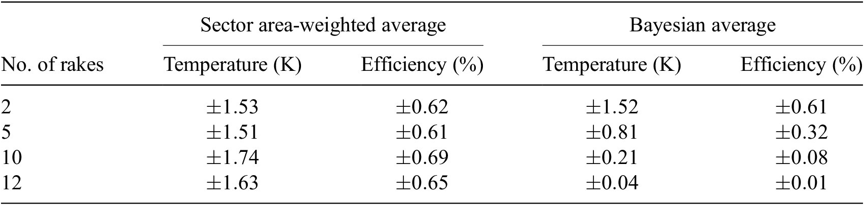
Note: All reported values are standard deviations based on Figure 10a,b.
This makes a compelling case for replacing the practice for computing area-averages in turbomachinery via sector weights with the proposed Bayesian treatment. As a side note, the idea of computing a Bayesian area average across an annulus has motivated the development of a more physically representative Bayesian mass average (see Seshadri et al., Reference Seshadri, Duncan and Thorne2022).
Next, we study the decomposition of the area-average variance in these randomized experiments and plot their spatial sampling and impact of measurement imprecision components (see (24) and (25)) in Figure 11. As before, the measurement noise is demarcated as a solid yellow line. There are interesting observations to make regarding these results.

Figure 11. Decomposition of area-average spatial sampling and impact of measurement imprecision area-average values for 40 randomized arrangements of rake positions.
First, the impact of measurement uncertainty increases with more instrumentation, till the model is able to adequately capture all the Fourier harmonics (after 11 rakes); we made an analogous finding when studying the spatial decomposition plots. This intuitively makes sense, as the more instrumentation we add, the greater the impact of measurement uncertainty. It is also worth noting that numerous rake arrangements can be found that curtail this source of uncertainty, many far below the threshold associated with the measurement noise.
Second, across the 40 rake configurations tested, spatial sampling uncertainty contributions were found to be very similar when using only two to three rakes. The variability in spatial sampling uncertainty decreases significantly when the number of rakes is sufficient to capture the circumferential harmonics. Thereafter, it is relatively constant, as observed by the collapsing of the red circles in Figure 11.
7. Transfer Learning Results with the Sparsity Promoting Prior
In this results section, we present the results of our inductive transfer learning framework with sparsity-promoting priors.
7.1. Transfer learning by splitting instrumentation
In this first case study, we consider traverse temperature measurements taken from a research turbine rig. Figure 12a shows the traverse locations at a temperature station, while Figure 12b shows the resulting steady-state temperature field. A fast Fourier transform was carried out on the temperature field at the hub, mid-span, and tip along the circumferential direction; the resulting amplitudes are captured in Figure 12c–e. It is clear that wave numbers 1, 12, and 24 are dominant. Additionally, we note that the signal is generally sparse, and thus utilization of the aforementioned sparsity-promoting priors seems like a sensible decision.

Figure 12. Experimental data from an exit station in a high-pressure turbine test rig: (a) traverse locations; (b) true temperature; Fourier amplitudes at the (c) hub, (d) mid-span, and (e) tip.
Let us assume that we can sample this spatial field using only 4 circumferential rakes, each fitted with 6 probes. Assume further that we are permitted to do this twice, with different circumferential rake placements. In both cases the rakes are clocked with respect to the upstream components, that is, they are aligned to be at the same pitchwise location, so as not to capture any upstream wakes.
Running the isolated plane model—that is, with no planar kernel—with sparsity promoting priors with $ \omega =\left(1,2,\dots, 15\right) $
for the first of the chosen rake arrangements, we obtain annular mean and standard deviation plots as shown in Figure 13a,b. While the posterior Gaussian random field does interpolate the measurements, by inspection it is readily apparent that the spatial pattern in Figure 13a does not match the truth in Figure 12b. Results run for the second rake arrangement are shown in Figure 13c,d.
$ \omega =\left(1,2,\dots, 15\right) $
for the first of the chosen rake arrangements, we obtain annular mean and standard deviation plots as shown in Figure 13a,b. While the posterior Gaussian random field does interpolate the measurements, by inspection it is readily apparent that the spatial pattern in Figure 13a does not match the truth in Figure 12b. Results run for the second rake arrangement are shown in Figure 13c,d.

Figure 13. Single plane calculations for the first rake arrangement (top row) and the second rake arrangement (bottom row). Posterior annular mean in (a,c); standard deviation in (b,d).
To ascertain if the transfer learning approach works, we pass these two rake arrangements as two separate measurement planes in the multi-plane model. As these measurements are from the same physical measurement station, they are both assigned the same value in the similarity vector, that is, $ \mathbf{s}=\left(1,1\right) $
. Once again, we resort to sparsity-promoting priors for inference. The results are shown in Figure 14. Beyond the greater resemblance to the truth in Figure 12b, a slight reduction in the spatial uncertainty is also observed. It is clear that the model has successfully transferred information across the two measurement planes to arrive at a more representative estimate of the temperature distribution. At the same time, the model still has sufficient flexibility to offer slightly different temperature distributions for each plane individually; as we will see in the next case study, this is an extremely useful characteristic.
$ \mathbf{s}=\left(1,1\right) $
. Once again, we resort to sparsity-promoting priors for inference. The results are shown in Figure 14. Beyond the greater resemblance to the truth in Figure 12b, a slight reduction in the spatial uncertainty is also observed. It is clear that the model has successfully transferred information across the two measurement planes to arrive at a more representative estimate of the temperature distribution. At the same time, the model still has sufficient flexibility to offer slightly different temperature distributions for each plane individually; as we will see in the next case study, this is an extremely useful characteristic.

Figure 14. Multi-plane calculations for the first rake arrangement (top row) and the second rake arrangement (bottom row). Posterior annular mean in (a,c); standard deviation in (b,d).
Circumferential plots of the single and the multi-plane yielded posterior distributions are contrasted in Figure 15 at the mid-span location; single plane results are shown in (a,c,e), while the multi-plane (inductive transfer learning) results are shown in (b,d,f). Subfigures (e) and (f) show the Fourier series amplitudes at the first plane only—these are very similar for the second plane. While it is apparent that in both cases the true pattern (shown with green circular markers) is well-captured within two standard deviations, in (b) and (d) the uncertainty is significantly reduced partly owing to the improved prediction of the mean. This comparison is important to emphasize, as it demonstrates the accuracy of the model’s predictions.

Figure 15. Comparison between the (a,c,e) single plane model and (b,d,f) the multi-plane transfer learning model at the mid-span location. Note that the amplitudes in (e) and (f) are only shown for the first planes (a) and (b). Green circular markers are the true values from the rig; blue markers represent a subset of four rakes.
7.2. Transfer learning with two adjacent planes from the same research engine
Next, we consider two temperature measurement planes located axially adjacent to each other in a research aeroengine. The first plane comprises 7 rakes each fitted with 7 radial temperature probes. The second plane comprises 24 thermocouples all placed at mid-span. As there are no rotating components between these two measurement stations, and owing to the fact that the flow is predominantly axial, it is hypothesized that they should have very similar temperature behavior.
The results of evaluating each measurement plane in isolation are captured in Figure 16 with circumferential distributions at mid-span for each plane. For these results, the sparsity priors were used with wave numbers $ \boldsymbol{\omega} =\left(1,2,\dots, 9\right) $
. This choice was set by the fact that the inclusion of wave numbers above 9 in the first plane leads to aliasing as the minimum angular distance between probes is 36°.
$ \boldsymbol{\omega} =\left(1,2,\dots, 9\right) $
. This choice was set by the fact that the inclusion of wave numbers above 9 in the first plane leads to aliasing as the minimum angular distance between probes is 36°.

Figure 16. Single model results for the first plane in (a,c,e) and the second plane in (b,d,f); here each plane was run individually.
It is clear that owing to the number of measurements in the second plane, there is little uncertainty in the overall circumferential distribution. The same cannot be said for the upstream stator plane in (a). Thus, the goal here is to explore whether the transfer learning enabled multi-plane model can (a) reduce the circumferential uncertainty in the first plane, whilst (b) reducing the radial uncertainty in the second plane.
As before, for the transfer learning model we set $ \mathbf{s}=\left(1,1\right) $
. Note that this explicitly assumes that both planes have the same set of wave numbers, although their precise amplitudes and phases may moderately differ, as stated before.
$ \mathbf{s}=\left(1,1\right) $
. Note that this explicitly assumes that both planes have the same set of wave numbers, although their precise amplitudes and phases may moderately differ, as stated before.
Figure 17 shows the results of the proposed model. It is clear that there is a reduction in the uncertainties in the radial direction in the burner plane, corresponding to the rake locations in the stator plane. There is also a significant reduction in the circumferential direction at mid-span region in the stator plane. Additionally, note how the radial distribution of temperature in the second plane resembles that seen on the first plane.

Figure 17. Multi-plane model results for the first plane in (a,c,e) and the second plane in (b,d,f).
7.3. Transfer learning across a fleet
One criticism of the work thus far is the reliance on s. Whilst in many cases, it is easy to establish whether two sets of measurements are similar, there may be equally many instances where such connections are difficult to draw. Ideally in such scenarios, it will be useful if the model itself can shed some light on the relative similarity between measurement planes, by virtue of radial and circumferential characteristics.
In this last example, we study the results of the multi-plane model on eight planes. The data chosen for this study corresponds to the temperature measurements taken from the same measurement at approximately the same throttle setting for eight different research engines. Planes E1–E3 belong to the same family, and planes E4, E5, and E7 belong to another family. Plane E8 is similar to E1–E3, but does have a different blade numbers. Additionally, planes E6 and E7 are more closely related to E4 and E5 than to planes E1–E3.
Rather than encode all these relationships in $ \mathbf{s} $
, we intentionally capture only the first few and set
$ \mathbf{s} $
, we intentionally capture only the first few and set $ \mathbf{s}=\left(\mathrm{1,1,1,2,2,3,4,5}\right) $
. From the resulting posterior distributions of
$ \mathbf{s}=\left(\mathrm{1,1,1,2,2,3,4,5}\right) $
. From the resulting posterior distributions of $ \eta $
and
$ \eta $
and $ {\xi}_1,\hskip0.35em \dots, \hskip0.35em {\xi}_W $
and their placement in
$ {\xi}_1,\hskip0.35em \dots, \hskip0.35em {\xi}_W $
and their placement in $ \boldsymbol{S} $
, we can construct the correlation matrix shown in Figure 18 by taking the mean of all the relevant hyperparameters
$ \boldsymbol{S} $
, we can construct the correlation matrix shown in Figure 18 by taking the mean of all the relevant hyperparameters $ \boldsymbol{\xi} $
. Subfigure (a) plots the mean of the correlation parameters, whilst (b) plots the standard deviation—bearing in mind that each iterate of the MCMC chain will yield a correlation matrix of this form. To reiterate, these correlation values stem from the constants in (9).
$ \boldsymbol{\xi} $
. Subfigure (a) plots the mean of the correlation parameters, whilst (b) plots the standard deviation—bearing in mind that each iterate of the MCMC chain will yield a correlation matrix of this form. To reiterate, these correlation values stem from the constants in (9).

Figure 18. A planar correlation plot for the posterior distributions of the parameters in $ \mathbf{S} $
: (a) mean; (b) standard deviation of MCMC samples (with burn-in removed).
$ \mathbf{S} $
: (a) mean; (b) standard deviation of MCMC samples (with burn-in removed).
From this correlation plot, we observe that many of the relationships previously mentioned but not captured in $ \mathbf{s} $
are apparent. For instance, E6 is observed to be more closely related to E4 and E5 respectively, compared to E1 (and by extension E2 and E3) with a value of 0.27. The model also rated E8’s similarity to E1 at 0.72, which seems reasonable given that both have a dominant mode four pattern. This value is higher than the correlation between E1, E2, and E3 and any of the other engines, which also aligns with our expectations. For completeness, we include the posterior mean distributions in Figure 19, where qualitatively one can observe a difference between engines that have a four-lobe versus a six-lobe pattern.
$ \mathbf{s} $
are apparent. For instance, E6 is observed to be more closely related to E4 and E5 respectively, compared to E1 (and by extension E2 and E3) with a value of 0.27. The model also rated E8’s similarity to E1 at 0.72, which seems reasonable given that both have a dominant mode four pattern. This value is higher than the correlation between E1, E2, and E3 and any of the other engines, which also aligns with our expectations. For completeness, we include the posterior mean distributions in Figure 19, where qualitatively one can observe a difference between engines that have a four-lobe versus a six-lobe pattern.

Figure 19. Posterior spatial means of the different planes.
8. Running Times and Code
All the results shown in this section and the next one were generated from a 2.6 GHz MacBook Pro with a dual core Intel i7 chip and with 64 GB of random access memory (RAM). All run time estimates provided are based on this machine configuration.
The underpinning GP framework was coded in python 3.8 using numpy (Harris et al., Reference Harris, Millman, van der Walt, Gommers, Virtanen, Cournapeau, Wieser, Taylor, Berg, Smith, Kern, Picus, Hoyer, van Kerkwijk, Brett, Haldane, del Río, Wiebe, Peterson, Gérard-Marchant, Sheppard, Reddy, Weckesser, Abbasi, Gohlke and Oliphant2020), scipy (Virtanen et al., Reference Virtanen, Gommers, Oliphant, Haberland, Reddy, Cournapeau, Burovski, Peterson, Weckesser, Bright, van der Walt, Brett, Wilson, Millman, Mayorov, Nelson, Jones, Kern, Larson, Carey, Polat, Feng, Moore, VanderPlas, Laxalde, Perktold, Cimrman, Henriksen, Quintero, Harris, Archibald, Ribeiro, Pedregosa and van Mulbregt2020), and pymc3 (Salvatier et al., Reference Salvatier, Wiecki and Fonnesbeck2016). The eight-plane transfer learning model took approximately 5 hr, while the two-plane transfer learning results took roughly 10 min. Both models assumed sparse priors. Single plane sparse MCMC results took under 5 min, while single plane simple prior (nonsparse) results took less than a minute. For all the MCMC results, we ran four chains in parallel.
9. Conclusions
Understanding the spatial annular pattern born from engine measurements provides valuable aerothermal insight. This article presents a transfer learning model suited for engine temperature and pressure measurements. It represents a step-up from prior averaging, uncertainty assessment, and spatial extrapolation works. Central to our contribution is the ability to transfer information across planes with a planar kernel and a user-defined input on the similarity between the different measurement planes. Beyond the results presented in this article, the proposed model has been extensively tested on measurement planes with 1–2 rakes of instrumentation when paired with planes with 6–7 rakes of instrumentation—with the goal of improving the spatial prediction even with 1–2 rakes. Across all cases, the multi-plane model yielded improved predictions. With respect to the proposed transfer learning model, future work could leverage Dirichlet prior models to learn S from data directly as part of the inference process.
Given the utility of the proposed model to test and measurement, future engine design, and engine health monitoring programmes, we anticipate many forthcoming advances within this modeling paradigm, especially for prognostic and diagnostic efforts.
Acknowledgment
The authors are grateful to Rolls-Royce plc for permission to publish this article.
Competing Interests
The authors declare no competing interests exist.
Data Availability Statement
The data that support the findings of this study is available from Rolls-Royce. Restrictions apply to the availability of this data.
Author Contributions
Conceptualization: P.S., A.B.D., G.T.; Data curation: P.S., G.T.; Data visualization: P.S.; Methodology: P.S., A.B.D., G.T.; Writing—original draft: P.S., A.B.D., G.T., G.P., R.V.D., M.G. All authors approved the final submitted draft.
Funding Statement
The work was partly funded by the Fan and Nacelle Future Aerodynamic Research (FANFARE) project under grant number 113286, which receives UK national funding through the Aerospace Technology Institute (ATI) and Innovate UK, together with work funded by Rolls-Royce plc.


 Open access
Comments
No Comments have been published for this article.