


1 Introduction
1.1 Statement of the main results
For a set $A\subset \mathbb{R}^{m}$
we define the algebraic part
$A\subset \mathbb{R}^{m}$
we define the algebraic part $A^{\text{alg}}$
of
$A^{\text{alg}}$
of $A$
to be the union of all connected semialgebraic subsets of
$A$
to be the union of all connected semialgebraic subsets of $A$
of positive dimension. We define the transcendental part
$A$
of positive dimension. We define the transcendental part $A^{\text{trans}}$
of
$A^{\text{trans}}$
of $A$
to be
$A$
to be $A\setminus A^{\text{alg}}$
.
$A\setminus A^{\text{alg}}$
.
Recall that the height of a (reduced) rational number $a/b\in \mathbb{Q}$
is defined to be
$a/b\in \mathbb{Q}$
is defined to be $\max (|a|,|b|)$
. For a vector
$\max (|a|,|b|)$
. For a vector $x$
of rational numbers we denote by
$x$
of rational numbers we denote by $H(x)$
the maximum among the heights of the coordinates. For a set
$H(x)$
the maximum among the heights of the coordinates. For a set $A\subset \mathbb{C}^{m}$
we denote the set of
$A\subset \mathbb{C}^{m}$
we denote the set of $\mathbb{Q}$
-points of
$\mathbb{Q}$
-points of $A$
by
$A$
by $A(\mathbb{Q}):=A\cap \mathbb{Q}^{m}$
and use the notation
$A(\mathbb{Q}):=A\cap \mathbb{Q}^{m}$
and use the notation
 $$\begin{eqnarray}A(\mathbb{Q},H):=\{x\in A(\mathbb{Q}):H(x)\leqslant H\}.\end{eqnarray}$$
For $A\subset \mathbb{R}^{m+n}$
and
$A\subset \mathbb{R}^{m+n}$
and $y\in \mathbb{R}^{n}$
we denote the
$y\in \mathbb{R}^{n}$
we denote the $y$
-fiber of
$y$
-fiber of $A$
by
$A$
by
 $$\begin{eqnarray}A_{y}\subset \mathbb{R}^{m},\quad A_{y}:=\{x\in \mathbb{R}^{m}:(x,y)\in A\}.\end{eqnarray}$$
In this paper we develop a new approach to the proof of the following theorem.
Theorem 1. Let $A\subset \mathbb{R}^{m+n}$
be a bounded subanalytic set and
$A\subset \mathbb{R}^{m+n}$
be a bounded subanalytic set and $\unicode[STIX]{x1D700}>0$
. There exists an integer
$\unicode[STIX]{x1D700}>0$
. There exists an integer $N(A,\unicode[STIX]{x1D700})$
such that for any
$N(A,\unicode[STIX]{x1D700})$
such that for any $y\in \mathbb{R}^{n}$
,
$y\in \mathbb{R}^{n}$
,
 $$\begin{eqnarray}\#(A_{y})^{\text{trans}}(\mathbb{Q},H)\leqslant N(A,\unicode[STIX]{x1D700})H^{\unicode[STIX]{x1D700}}.\end{eqnarray}$$
The result of Theorem 1 is not new. In fact, it was conjectured in [Reference PilaPil04, Conjecture 1.2] and proved, in a more general form, in the work of Pila and Wilkie [Reference Pila and WilkiePW06], where the same result is shown to hold for any $A$
definable in an O-minimal structure. Our goal in the present paper is to develop an alternative complex analytic approach to this theorem. In particular, while the proof in [Reference Pila and WilkiePW06] requires the use of
$A$
definable in an O-minimal structure. Our goal in the present paper is to develop an alternative complex analytic approach to this theorem. In particular, while the proof in [Reference Pila and WilkiePW06] requires the use of $C^{r}$
parametrizations of subanalytic sets, we are able to carry out the arguments completely within the analytic category. The proof of Theorem 1 is given at the end of § 5.3. As a first illustration of the advantage of this approach, we prove the following complex analog of a recent result of [Reference Cluckers, Pila and WilkieCPW16].
$C^{r}$
parametrizations of subanalytic sets, we are able to carry out the arguments completely within the analytic category. The proof of Theorem 1 is given at the end of § 5.3. As a first illustration of the advantage of this approach, we prove the following complex analog of a recent result of [Reference Cluckers, Pila and WilkieCPW16].
Theorem 2 (Cf. [Reference Cluckers, Pila and WilkieCPW16, Theorem 2.3.2]).
Let $X\subset \mathbb{C}^{m+n}$
be a locally analytic subset and
$X\subset \mathbb{C}^{m+n}$
be a locally analytic subset and $K\Subset X$
be a compact subset. Suppose
$K\Subset X$
be a compact subset. Suppose $\dim _{\mathbb{C}}X_{y}\leqslant k$
for every
$\dim _{\mathbb{C}}X_{y}\leqslant k$
for every $y\in \mathbb{C}^{n}$
. Then there exists a constant
$y\in \mathbb{C}^{n}$
. Then there exists a constant $C=C(K)$
such that for any
$C=C(K)$
such that for any $y\in \mathbb{C}^{n}$
, if
$y\in \mathbb{C}^{n}$
, if $H>2$
, then
$H>2$
, then $K_{y}(\mathbb{Q},H)$
is contained in the union of at most
$K_{y}(\mathbb{Q},H)$
is contained in the union of at most $C$
complex algebraic hypersurfaces of degree at most
$C$
complex algebraic hypersurfaces of degree at most $(\log H)^{k/(m-k)}$
in
$(\log H)^{k/(m-k)}$
in $\mathbb{C}^{m}$
.
$\mathbb{C}^{m}$
.
The proof of Theorem 2 is given following Corollary 13. In [Reference Cluckers, Pila and WilkieCPW16, Theorem 2.3.2] a result similar to Theorem 2 is stated for real globally subanalytic sets. The dimensions are taken over $\mathbb{R}$
and the algebraic hypersurfaces constructed are real. We give the complex version for variation, and also since in most applications the sets involved are, in fact, complex analytic. Note that in this case the complex analytic version gives more than the real version: the degree of the hypersurface is the same as in [Reference Cluckers, Pila and WilkieCPW16, Theorem 2.3.2], but intersecting with a complex-algebraic hypersurface imposes two independent real-algebraic conditions. We also remark that the real version [Reference Cluckers, Pila and WilkieCPW16, Theorem 2.3.2] could also be derived with our method by the same complexification arguments used in our proof of Theorem 1.
$\mathbb{R}$
and the algebraic hypersurfaces constructed are real. We give the complex version for variation, and also since in most applications the sets involved are, in fact, complex analytic. Note that in this case the complex analytic version gives more than the real version: the degree of the hypersurface is the same as in [Reference Cluckers, Pila and WilkieCPW16, Theorem 2.3.2], but intersecting with a complex-algebraic hypersurface imposes two independent real-algebraic conditions. We also remark that the real version [Reference Cluckers, Pila and WilkieCPW16, Theorem 2.3.2] could also be derived with our method by the same complexification arguments used in our proof of Theorem 1.
Our principal motivation for the complex-analytic approach developed in this paper is the Wilkie conjecture on the improvement of the asymptotic $O(H^{\unicode[STIX]{x1D700}})$
to polylogarithmic for certain structures (see § 1.2 for details). Theorem 2 can be seen as a natural first inductive step toward this conjecture. However, pursuing this induction further requires analyzing the behavior of the constant
$O(H^{\unicode[STIX]{x1D700}})$
to polylogarithmic for certain structures (see § 1.2 for details). Theorem 2 can be seen as a natural first inductive step toward this conjecture. However, pursuing this induction further requires analyzing the behavior of the constant $C(A)$
with respect to the complexity of the set
$C(A)$
with respect to the complexity of the set $A$
; a problem which requires finer analysis that cannot be carried out in the generality of general analytic sets (as illustrated by counterexamples due to Pila [Reference PilaPil04, Example 7.5]). In a closely related preprint [Reference Binyamini and NovikovBN17] we build on the ideas developed in this paper to prove the Wilkie conjecture for sets definable using the restricted exponential and sine functions; a problem which had previously seemed quite challenging due to the difficulty of computing
$A$
; a problem which requires finer analysis that cannot be carried out in the generality of general analytic sets (as illustrated by counterexamples due to Pila [Reference PilaPil04, Example 7.5]). In a closely related preprint [Reference Binyamini and NovikovBN17] we build on the ideas developed in this paper to prove the Wilkie conjecture for sets definable using the restricted exponential and sine functions; a problem which had previously seemed quite challenging due to the difficulty of computing $C^{r}$
parametrizations.
$C^{r}$
parametrizations.
In § 1.2 we present some motivations for our approach. In § 1.3 we briefly review the method of Bombieri–Pila–Wilkie and, in particular, explain the point at which $C^{r}$
-parametrizations are required. In § 1.4 we give an outline of the complex-analytic approach developed in this paper and explain how it avoids the use of
$C^{r}$
-parametrizations are required. In § 1.4 we give an outline of the complex-analytic approach developed in this paper and explain how it avoids the use of $C^{r}$
-parametrizations.
$C^{r}$
-parametrizations.
Note.
Shortly after the appearance of the first version of this manuscript (and the closely related preprint [Reference Binyamini and NovikovBN17]) on the arXiv, the independently developed preprint [Reference Cluckers, Pila and WilkieCPW16] by Cluckers, Pila and Wilkie appeared. Some of the methods appear to be related: in particular the ‘quasi-parametrization theorem’ [Reference Cluckers, Pila and WilkieCPW16, Theorem 2.2.3] appears similar to our notion of a decomposition datum, and the diophantine application [Reference Cluckers, Pila and WilkieCPW16, Theorem 2.3.2] is also a consequence of our approach. We wish to clarify that Theorem 2 was not included in the original version of this manuscript and appeared (in the real version) originally in [Reference Cluckers, Pila and WilkieCPW16]; in a later version we included the complex Theorem 2 to illustrate how our approach can be used to derive similar results.
1.2 Motivation
There are two directions in which one might hope to improve the Pila–Wilkie estimate $\#A^{\text{trans}}(\mathbb{Q},H)\leqslant N(A,\unicode[STIX]{x1D700})H^{\unicode[STIX]{x1D700}}$
.
$\#A^{\text{trans}}(\mathbb{Q},H)\leqslant N(A,\unicode[STIX]{x1D700})H^{\unicode[STIX]{x1D700}}$
.
-
∙ Effective estimates: one may hope to obtain effective estimates for the constant $N(A,\unicode[STIX]{x1D700})$
in terms of the complexity of the equations/formulas used to define
$A$
.
$N(A,\unicode[STIX]{x1D700})$
in terms of the complexity of the equations/formulas used to define
$A$
. -
∙ Sharper asymptotics: one may hope to improve the asymptotic dependence on
$H$
if
$A$
is definable in a suitably tame structure. As a notable example, the Wilkie conjecture states that if
$A$
is definable in
$\mathbb{R}_{\exp }$
, then
$\#A^{\text{trans}}(\mathbb{Q},H)=N(A)(\log H)^{\unicode[STIX]{x1D705}(A)}$
.


Both of these directions have been considered in the literature, see e.g. [Reference ButlerBut12, Reference Jones and ThomasJT12, Reference PilaPil10, Reference PilaPil07]. However, as discussed in § 1.3, the proof of the Pila–Wilkie theorem in arbitrary dimensions requires the use of $C^{r}$
-reparametrizations, whose complexity is difficult to control even in the semialgebraic case. For this reason, most of the work (to the best of the authors’ knowledge) has been restricted to
$C^{r}$
-reparametrizations, whose complexity is difficult to control even in the semialgebraic case. For this reason, most of the work (to the best of the authors’ knowledge) has been restricted to $A$
of (real) dimension one or two.
$A$
of (real) dimension one or two.
Our primary goal in this paper is to develop an approach that replaces the use of $C^{r}$
-parametrization by direct considerations on the local complex-analytic geometry of
$C^{r}$
-parametrization by direct considerations on the local complex-analytic geometry of $A$
. In the preprint [Reference Binyamini and NovikovBN17] we use this approach to prove the Wilkie conjecture for sets definable using the restricted exponential and sine functions, where Proposition 11 provides the key inductive step. The estimates in [Reference Binyamini and NovikovBN17] are also effective in a suitable sense. We believe that the analytic approach may also play a significant role in advancing toward an effective version of the Pila–Wilkie theorem for Noetherian functions.
$A$
. In the preprint [Reference Binyamini and NovikovBN17] we use this approach to prove the Wilkie conjecture for sets definable using the restricted exponential and sine functions, where Proposition 11 provides the key inductive step. The estimates in [Reference Binyamini and NovikovBN17] are also effective in a suitable sense. We believe that the analytic approach may also play a significant role in advancing toward an effective version of the Pila–Wilkie theorem for Noetherian functions.
Finally, while in this paper we work in the complex analytic setting, our arguments are essentially algebraic; tracing to the Weierstrass preparation and division theorems. One may hope that such an approach could allow a more direct generalization to different algebraic contexts where the analytic notion of $C^{r}$
-parametrization may be more difficult to recover. In particular, we consider it an interesting direction to check whether the method developed in this paper can offer an alternative approach to the work of Cluckers et al. [Reference Cluckers, Comte and LoeserCCL15] on non-archimedean analogs of the Pila–Wilkie theorem. We remark in this context that in our primary model-theoretic reference [Reference Denef and van den DriesDvdD88], the complex-analytic and
$C^{r}$
-parametrization may be more difficult to recover. In particular, we consider it an interesting direction to check whether the method developed in this paper can offer an alternative approach to the work of Cluckers et al. [Reference Cluckers, Comte and LoeserCCL15] on non-archimedean analogs of the Pila–Wilkie theorem. We remark in this context that in our primary model-theoretic reference [Reference Denef and van den DriesDvdD88], the complex-analytic and $p$
-adic contexts are treated in close analogy.
$p$
-adic contexts are treated in close analogy.
1.3 Exploring rational points following Bombieri–Pila and Pila–Wilkie
1.3.1 The case of curves
Let $X\subset \mathbb{R}^{2}$
be compact irreducible real-analytic curve. Building upon earlier work by Bombieri and Pila [Reference Bombieri and PilaBP89], Pila [Reference PilaPil91] considered the problem of estimating
$X\subset \mathbb{R}^{2}$
be compact irreducible real-analytic curve. Building upon earlier work by Bombieri and Pila [Reference Bombieri and PilaBP89], Pila [Reference PilaPil91] considered the problem of estimating $\#X(\mathbb{Q},H)$
. More specifically, he showed that if
$\#X(\mathbb{Q},H)$
. More specifically, he showed that if $X$
is transcendental, then for every
$X$
is transcendental, then for every $\unicode[STIX]{x1D700}>0$
there exists a constant
$\unicode[STIX]{x1D700}>0$
there exists a constant $C(X,\unicode[STIX]{x1D700})$
such that
$C(X,\unicode[STIX]{x1D700})$
such that $\#X(\mathbb{Q},H)\leqslant C(X,\unicode[STIX]{x1D700})H^{\unicode[STIX]{x1D700}}$
. Bombieri and Pila’s method involves constructing a collection of
$\#X(\mathbb{Q},H)\leqslant C(X,\unicode[STIX]{x1D700})H^{\unicode[STIX]{x1D700}}$
. Bombieri and Pila’s method involves constructing a collection of $H^{\unicode[STIX]{x1D700}}$
hypersurfaces
$H^{\unicode[STIX]{x1D700}}$
hypersurfaces $\{H_{k}\}$
of degree
$\{H_{k}\}$
of degree $d=d(\unicode[STIX]{x1D700})$
such that
$d=d(\unicode[STIX]{x1D700})$
such that $X(\mathbb{Q},H)$
is contained in
$X(\mathbb{Q},H)$
is contained in $\bigcup _{k}H_{k}$
. We briefly recall the key idea, starting with the notion of an interpolation determinant.
$\bigcup _{k}H_{k}$
. We briefly recall the key idea, starting with the notion of an interpolation determinant.
Suppose first that $X$
can be written as the image of an analytic map
$X$
can be written as the image of an analytic map $\mathbf{f}=(f_{1},f_{2}):[0,1]\rightarrow X$
(the general case will be treated later by subdivision). For simplicity, we will suppose that
$\mathbf{f}=(f_{1},f_{2}):[0,1]\rightarrow X$
(the general case will be treated later by subdivision). For simplicity, we will suppose that $f_{1},f_{2}$
extend to holomorphic functions in the disc of radius
$f_{1},f_{2}$
extend to holomorphic functions in the disc of radius $2$
around the origin, with absolute value bounded by
$2$
around the origin, with absolute value bounded by $M$
.
$M$
.
Let $\mathbf{g}:=(g_{1},\ldots ,g_{\unicode[STIX]{x1D707}})$
be a collection of functions and
$\mathbf{g}:=(g_{1},\ldots ,g_{\unicode[STIX]{x1D707}})$
be a collection of functions and $\mathbf{p}:=(p_{1},\ldots ,p_{\unicode[STIX]{x1D707}})$
a collection of points. We define the interpolation determinant
$\mathbf{p}:=(p_{1},\ldots ,p_{\unicode[STIX]{x1D707}})$
a collection of points. We define the interpolation determinant
 $$\begin{eqnarray}\unicode[STIX]{x1D6E5}(\mathbf{g},\mathbf{p}):=\det (g_{i}(p_{j}))_{1\leqslant i,j\leqslant \unicode[STIX]{x1D707}}.\end{eqnarray}$$
Let $d\in \mathbb{N}$
and set
$d\in \mathbb{N}$
and set $\unicode[STIX]{x1D707}=d(d+1)/2$
, the dimension of the space of polynomials in two variables of degree at most
$\unicode[STIX]{x1D707}=d(d+1)/2$
, the dimension of the space of polynomials in two variables of degree at most $d$
. We define the polynomial interpolation determinant of degree
$d$
. We define the polynomial interpolation determinant of degree $d$
to be
$d$
to be
 $$\begin{eqnarray}\unicode[STIX]{x1D6E5}^{d}(\mathbf{f},\mathbf{p}):=\unicode[STIX]{x1D6E5}(\mathbf{g},\mathbf{p}),\quad \mathbf{g}=(f_{1}^{k}f_{2}^{l}:k,l\in \mathbb{N},~k+l\leqslant d).\end{eqnarray}$$
Note that $\unicode[STIX]{x1D6E5}^{d}(\mathbf{f},\mathbf{p})=0$
if and only if the points
$\unicode[STIX]{x1D6E5}^{d}(\mathbf{f},\mathbf{p})=0$
if and only if the points $\mathbf{f}(p_{1}),\ldots ,\mathbf{f}(p_{\unicode[STIX]{x1D707}})$
all lie on a common algebraic hypersurface of degree at most
$\mathbf{f}(p_{1}),\ldots ,\mathbf{f}(p_{\unicode[STIX]{x1D707}})$
all lie on a common algebraic hypersurface of degree at most $d$
. More generally, if
$d$
. More generally, if $P\subset I$
and
$P\subset I$
and $\unicode[STIX]{x1D6E5}^{d}(\mathbf{f},\mathbf{p})=0$
for every
$\unicode[STIX]{x1D6E5}^{d}(\mathbf{f},\mathbf{p})=0$
for every $\mathbf{p}\subset P$
, then the points
$\mathbf{p}\subset P$
, then the points $\mathbf{f}(p):p\in P$
all lie on a common algebraic hypersurface of degree at most
$\mathbf{f}(p):p\in P$
all lie on a common algebraic hypersurface of degree at most $d$
.
$d$
.
Let $H\in \mathbb{N}$
. Our goal is to construct a collection of algebraic hypersurfaces
$H\in \mathbb{N}$
. Our goal is to construct a collection of algebraic hypersurfaces $H_{k}$
whose union contains
$H_{k}$
whose union contains $X(\mathbb{Q},H)$
. By the above, it will suffice to subdivide
$X(\mathbb{Q},H)$
. By the above, it will suffice to subdivide $I$
into intervals
$I$
into intervals $I_{k}$
such that for any
$I_{k}$
such that for any $\mathbf{p}\subset I_{k}$
, if
$\mathbf{p}\subset I_{k}$
, if $H(\mathbf{p})\leqslant H$
, then
$H(\mathbf{p})\leqslant H$
, then $\unicode[STIX]{x1D6E5}^{d}(\mathbf{f},\mathbf{p})=0$
. We begin with the following key estimate on the polynomial interpolation determinant.
$\unicode[STIX]{x1D6E5}^{d}(\mathbf{f},\mathbf{p})=0$
. We begin with the following key estimate on the polynomial interpolation determinant.
Lemma 1 (Cf. Lemma 9).
Let $I\,\subset \,[0,1]$
be an interval of length
$I\,\subset \,[0,1]$
be an interval of length $\unicode[STIX]{x1D6FF}\,<\,1/2$
, and
$\unicode[STIX]{x1D6FF}\,<\,1/2$
, and $\mathbf{p}\,=\,(p_{1},\ldots ,p_{\unicode[STIX]{x1D707}})\in I^{\unicode[STIX]{x1D707}}$
. Then
$\mathbf{p}\,=\,(p_{1},\ldots ,p_{\unicode[STIX]{x1D707}})\in I^{\unicode[STIX]{x1D707}}$
. Then
 $$\begin{eqnarray}|\unicode[STIX]{x1D6E5}^{d}(\mathbf{f},\mathbf{p})|\leqslant \unicode[STIX]{x1D707}!(2\unicode[STIX]{x1D707}+2)^{\unicode[STIX]{x1D707}}M^{d\unicode[STIX]{x1D707}}\unicode[STIX]{x1D6FF}^{\unicode[STIX]{x1D707}^{2}/2}.\end{eqnarray}$$
Proof. By translation we may suppose that $I=[-\unicode[STIX]{x1D6FF},\unicode[STIX]{x1D6FF}]$
and that
$I=[-\unicode[STIX]{x1D6FF},\unicode[STIX]{x1D6FF}]$
and that $f_{1},f_{2}$
are holomorphic in the unit disc
$f_{1},f_{2}$
are holomorphic in the unit disc $D\subset \mathbb{C}$
with absolute value bounded by
$D\subset \mathbb{C}$
with absolute value bounded by $M$
. Denote by
$M$
. Denote by $\Vert \cdot \Vert$
the maximum norm on the disc of radius
$\Vert \cdot \Vert$
the maximum norm on the disc of radius $\unicode[STIX]{x1D6FF}$
around the origin.
$\unicode[STIX]{x1D6FF}$
around the origin.
Every function in $\mathbf{g}$
is holomorphic in
$\mathbf{g}$
is holomorphic in $D$
with absolute value bounded by
$D$
with absolute value bounded by $M^{d}$
. Consider the Taylor expansions
$M^{d}$
. Consider the Taylor expansions
 $$\begin{eqnarray}g_{i}=\mathop{\sum }_{j=0}^{\unicode[STIX]{x1D707}-1}m_{j}(g_{i})+R_{\unicode[STIX]{x1D707}}(g_{i}),\quad m_{j}(g_{i}):=c_{i,j}x^{j},\;i=1,\ldots ,\unicode[STIX]{x1D707}\end{eqnarray}$$
and $R_{j}(g_{i})$
are the Taylor residues. From the Cauchy estimates we have
$R_{j}(g_{i})$
are the Taylor residues. From the Cauchy estimates we have
 $$\begin{eqnarray}\Vert m_{j}(g_{i})\Vert \leqslant M^{d}\unicode[STIX]{x1D6FF}^{j},\quad \Vert R_{\unicode[STIX]{x1D707}}(g_{i})\Vert \leqslant 2M^{d}\unicode[STIX]{x1D6FF}^{\unicode[STIX]{x1D707}}.\end{eqnarray}$$
Expand the determinant $\unicode[STIX]{x1D6E5}^{d}(\mathbf{f},\mathbf{p})$
by linearity using (7), to obtain a sum of
$\unicode[STIX]{x1D6E5}^{d}(\mathbf{f},\mathbf{p})$
by linearity using (7), to obtain a sum of $(\unicode[STIX]{x1D707}+1)^{\unicode[STIX]{x1D707}}$
summands with each
$(\unicode[STIX]{x1D707}+1)^{\unicode[STIX]{x1D707}}$
summands with each $g_{i}$
replaced by either
$g_{i}$
replaced by either $m_{j_{i}}(g_{i})$
or
$m_{j_{i}}(g_{i})$
or $R_{\unicode[STIX]{x1D707}}(g_{i})$
. Note that any summand where two different indices
$R_{\unicode[STIX]{x1D707}}(g_{i})$
. Note that any summand where two different indices $j_{k},j_{l}$
agree vanishes identically since the corresponding functions
$j_{k},j_{l}$
agree vanishes identically since the corresponding functions $m_{j_{k}}(g_{k}),m_{j_{l}}(g_{l})$
are linearly dependent. Therefore, any non-zero summand must contain a term of order at least one, a term of order at least two, and so on. Then an easy computation using (8) and the Laplace expansion for each determinant gives (6).◻
$m_{j_{k}}(g_{k}),m_{j_{l}}(g_{l})$
are linearly dependent. Therefore, any non-zero summand must contain a term of order at least one, a term of order at least two, and so on. Then an easy computation using (8) and the Laplace expansion for each determinant gives (6).◻
Let $I,\mathbf{p}$
be as in Lemma 1 and suppose
$I,\mathbf{p}$
be as in Lemma 1 and suppose $\mathbf{f}(p_{1}),\ldots ,\mathbf{f}(p_{\unicode[STIX]{x1D707}})\in X(\mathbb{Q},H)$
. Using the bounded heights of
$\mathbf{f}(p_{1}),\ldots ,\mathbf{f}(p_{\unicode[STIX]{x1D707}})\in X(\mathbb{Q},H)$
. Using the bounded heights of $\mathbf{f}(p_{j})$
one proves (cf. Lemma 10) that either
$\mathbf{f}(p_{j})$
one proves (cf. Lemma 10) that either $\unicode[STIX]{x1D6E5}^{d}(f,\mathbf{p})=0$
or
$\unicode[STIX]{x1D6E5}^{d}(f,\mathbf{p})=0$
or
 $$\begin{eqnarray}|\unicode[STIX]{x1D6E5}^{d}(f,\mathbf{p})|\geqslant H^{-O(d^{3})}.\end{eqnarray}$$
Comparing (6) and (9) and recalling that $\unicode[STIX]{x1D707}\sim d^{2}$
we have either
$\unicode[STIX]{x1D707}\sim d^{2}$
we have either $\unicode[STIX]{x1D6E5}^{d}(f,\mathbf{p})=0$
or
$\unicode[STIX]{x1D6E5}^{d}(f,\mathbf{p})=0$
or
 $$\begin{eqnarray}H^{-O(d^{3})}\leqslant |\unicode[STIX]{x1D6E5}^{d}(f,\mathbf{p})|\leqslant 2^{O(d^{3})}\unicode[STIX]{x1D6FF}^{\unicode[STIX]{x1D6FA}(d^{4})},\end{eqnarray}$$
where we treat $M$
as
$M$
as $O(1)$
. Thus, if
$O(1)$
. Thus, if $\unicode[STIX]{x1D6FF}=H^{-\unicode[STIX]{x1D6FA}(1/d)}$
, then
$\unicode[STIX]{x1D6FF}=H^{-\unicode[STIX]{x1D6FA}(1/d)}$
, then $\unicode[STIX]{x1D6E5}^{d}(f,\mathbf{p})$
must vanish for any
$\unicode[STIX]{x1D6E5}^{d}(f,\mathbf{p})$
must vanish for any $\mathbf{p}$
as above. Thus, as explained above, all points
$\mathbf{p}$
as above. Thus, as explained above, all points $\mathbf{f}(p)\in X(\mathbb{Q},H)$
with
$\mathbf{f}(p)\in X(\mathbb{Q},H)$
with $p\in I$
belong to a single algebraic hypersurface
$p\in I$
belong to a single algebraic hypersurface $H_{k}\subset \mathbb{R}^{2}$
of degree at most
$H_{k}\subset \mathbb{R}^{2}$
of degree at most $d$
.
$d$
.
Fix $\unicode[STIX]{x1D700}>0$
and subdivide
$\unicode[STIX]{x1D700}>0$
and subdivide $I$
into
$I$
into $H^{\unicode[STIX]{x1D700}}$
subintervals
$H^{\unicode[STIX]{x1D700}}$
subintervals $I_{k}$
of length
$I_{k}$
of length $\unicode[STIX]{x1D6FF}=H^{-\unicode[STIX]{x1D700}}$
. Then, by the above, all points of
$\unicode[STIX]{x1D6FF}=H^{-\unicode[STIX]{x1D700}}$
. Then, by the above, all points of $X(\mathbb{Q},H)$
belong to a union of
$X(\mathbb{Q},H)$
belong to a union of $H^{\unicode[STIX]{x1D700}}$
hypersurfaces
$H^{\unicode[STIX]{x1D700}}$
hypersurfaces $H_{k}\subset \mathbb{R}^{2}$
of degree
$H_{k}\subset \mathbb{R}^{2}$
of degree $d=O(1/\unicode[STIX]{x1D700})$
. If
$d=O(1/\unicode[STIX]{x1D700})$
. If $X$
is irreducible and transcendental, then it intersects each
$X$
is irreducible and transcendental, then it intersects each $H_{k}$
properly, and the number of intersections between
$H_{k}$
properly, and the number of intersections between $X$
and
$X$
and $H_{k}$
is uniformly bounded by some constant
$H_{k}$
is uniformly bounded by some constant $C(X,d)$
depending only on
$C(X,d)$
depending only on $X$
and
$X$
and $d$
(for instance, by Gabrielov’s theorem). Thus, we have
$d$
(for instance, by Gabrielov’s theorem). Thus, we have $\#X(\mathbb{Q},H)\leqslant C(X,\unicode[STIX]{x1D700})H^{\unicode[STIX]{x1D700}}$
.
$\#X(\mathbb{Q},H)\leqslant C(X,\unicode[STIX]{x1D700})H^{\unicode[STIX]{x1D700}}$
.
To handle the case of a general compact irreducible analytic curve $X\subset \mathbb{R}^{2}$
we note that any such curve can be covered by images of analytic maps
$X\subset \mathbb{R}^{2}$
we note that any such curve can be covered by images of analytic maps $\mathbf{f}:[0,1]\rightarrow X$
and the preceding arguments apply.
$\mathbf{f}:[0,1]\rightarrow X$
and the preceding arguments apply.
1.3.2 Higher dimensions
It is natural to attempt to generalize the proof of § 1.3.1 to sets $X\subset \mathbb{R}^{m}$
of dimension
$X\subset \mathbb{R}^{m}$
of dimension $\ell >1$
by induction over
$\ell >1$
by induction over $\ell$
. Namely, the estimates (6) and (9) can be generalized in a relatively straightforward manner, replacing the map
$\ell$
. Namely, the estimates (6) and (9) can be generalized in a relatively straightforward manner, replacing the map $\mathbf{f}:(0,1)\rightarrow X$
by an arbitrary analytic map
$\mathbf{f}:(0,1)\rightarrow X$
by an arbitrary analytic map $\mathbf{f}:(0,1)^{\ell }\rightarrow X$
parametrizing an
$\mathbf{f}:(0,1)^{\ell }\rightarrow X$
parametrizing an $\ell$
-dimensional set
$\ell$
-dimensional set $X$
. One similarly obtains
$X$
. One similarly obtains $H^{\unicode[STIX]{x1D700}}$
hypersurfaces
$H^{\unicode[STIX]{x1D700}}$
hypersurfaces $H_{k}$
of some fixed degree
$H_{k}$
of some fixed degree $d=d(\unicode[STIX]{x1D700})$
such that
$d=d(\unicode[STIX]{x1D700})$
such that
 $$\begin{eqnarray}X(\mathbb{Q},H)\subset \mathop{\bigcup }_{k}X\cap H_{k}.\end{eqnarray}$$
One would then seek to continue treating each intersection $X\cap H_{k}$
by induction on the dimension. However, at this point a problem arises: even if the original set
$X\cap H_{k}$
by induction on the dimension. However, at this point a problem arises: even if the original set $X$
was parametrized by an analytic map
$X$
was parametrized by an analytic map $\mathbf{f}:(0,1)^{\ell }\rightarrow X$
it is not clear that
$\mathbf{f}:(0,1)^{\ell }\rightarrow X$
it is not clear that $X\cap H_{k}$
could be parametrized in a similar manner. Moreover, if one does obtain a parametrization for each intersection
$X\cap H_{k}$
could be parametrized in a similar manner. Moreover, if one does obtain a parametrization for each intersection $X\cap H_{k}$
, then the induction constant
$X\cap H_{k}$
, then the induction constant $C(X\cap H_{k},\unicode[STIX]{x1D700})$
would now depend on the specific parametrizations chosen for
$C(X\cap H_{k},\unicode[STIX]{x1D700})$
would now depend on the specific parametrizations chosen for $X\cap H_{k}$
, and one must show that these constants are uniformly bounded over all
$X\cap H_{k}$
, and one must show that these constants are uniformly bounded over all $H_{k}$
of the given degree
$H_{k}$
of the given degree $d$
.
$d$
.
In fact, it is not always possible to choose analytic, or even $C^{\infty }$
-smooth, parametrizations for the fibers of a family in a uniform manner; even for semialgebraic families of curves. This fundamental limitation was observed in the work of Yomdin [Reference YomdinYom87a]. Consider for example the family of hyperbolas
$C^{\infty }$
-smooth, parametrizations for the fibers of a family in a uniform manner; even for semialgebraic families of curves. This fundamental limitation was observed in the work of Yomdin [Reference YomdinYom87a]. Consider for example the family of hyperbolas $X_{\unicode[STIX]{x1D700}}:=(-1,1)^{2}\cap \{x^{2}-y^{2}=\unicode[STIX]{x1D700}\}$
. If one attempts to write
$X_{\unicode[STIX]{x1D700}}:=(-1,1)^{2}\cap \{x^{2}-y^{2}=\unicode[STIX]{x1D700}\}$
. If one attempts to write $X_{\unicode[STIX]{x1D700}}$
as a union of images
$X_{\unicode[STIX]{x1D700}}$
as a union of images $\operatorname{Im}\unicode[STIX]{x1D719}_{j}$
for
$\operatorname{Im}\unicode[STIX]{x1D719}_{j}$
for $C^{\infty }$
-smooth functions
$C^{\infty }$
-smooth functions $\unicode[STIX]{x1D719}_{1},\ldots ,\unicode[STIX]{x1D719}_{N_{\unicode[STIX]{x1D700}}}:(0,1)\rightarrow X_{\unicode[STIX]{x1D700}}$
with the maximum norms of the derivatives of every order bounded by
$\unicode[STIX]{x1D719}_{1},\ldots ,\unicode[STIX]{x1D719}_{N_{\unicode[STIX]{x1D700}}}:(0,1)\rightarrow X_{\unicode[STIX]{x1D700}}$
with the maximum norms of the derivatives of every order bounded by $1$
, then
$1$
, then $N_{\unicode[STIX]{x1D700}}$
necessarily tends to infinity as
$N_{\unicode[STIX]{x1D700}}$
necessarily tends to infinity as $\unicode[STIX]{x1D700}\rightarrow 0$
. Thus, it would not be possible to parametrize all fibers of this family in a uniform manner and apply to them the methods of § 1.3.1.
$\unicode[STIX]{x1D700}\rightarrow 0$
. Thus, it would not be possible to parametrize all fibers of this family in a uniform manner and apply to them the methods of § 1.3.1.
Surprisingly, a theorem due to Yomdin and Gromov [Reference YomdinYom87a, Reference YomdinYom87b, Reference GromovGro87] states that one can recover the uniformity of $N_{\unicode[STIX]{x1D700}}$
if one replaces the
$N_{\unicode[STIX]{x1D700}}$
if one replaces the $C^{\infty }$
condition by
$C^{\infty }$
condition by $C^{r}$
-smoothness for a fixed
$C^{r}$
-smoothness for a fixed $r$
, at least for semialgebraic families. In [Reference Pila and WilkiePW06], Pila and Wilkie generalized this result to the O-minimal setting. Namely, they show [Reference Pila and WilkiePW06, Corollary 5.1] that for any set
$r$
, at least for semialgebraic families. In [Reference Pila and WilkiePW06], Pila and Wilkie generalized this result to the O-minimal setting. Namely, they show [Reference Pila and WilkiePW06, Corollary 5.1] that for any set $X\subset (0,1)^{m}$
of dimension
$X\subset (0,1)^{m}$
of dimension $\ell$
definable in an O-minimal structure and any
$\ell$
definable in an O-minimal structure and any $r\in \mathbb{N}$
, one can cover
$r\in \mathbb{N}$
, one can cover $X$
by images of
$X$
by images of $C^{r}$
-maps
$C^{r}$
-maps $\unicode[STIX]{x1D719}_{1},\ldots ,\unicode[STIX]{x1D719}_{N}:(0,1)^{\ell }\rightarrow X$
where
$\unicode[STIX]{x1D719}_{1},\ldots ,\unicode[STIX]{x1D719}_{N}:(0,1)^{\ell }\rightarrow X$
where $N=N(X,r)$
and every
$N=N(X,r)$
and every $\unicode[STIX]{x1D719}_{j}$
has
$\unicode[STIX]{x1D719}_{j}$
has $C^{r}$
-norm bounded by
$C^{r}$
-norm bounded by $1$
in
$1$
in $(0,1)^{\ell }$
. Moreover (see [Reference Pila and WilkiePW06, Corollary 5.2]), if
$(0,1)^{\ell }$
. Moreover (see [Reference Pila and WilkiePW06, Corollary 5.2]), if $X$
varies in a definable family (and
$X$
varies in a definable family (and $r$
is fixed), then
$r$
is fixed), then $N$
can be taken to be uniformly bounded over the entire family.
$N$
can be taken to be uniformly bounded over the entire family.
One can now check that in the proof sketched in § 1.3.1 the analyticity assumption can be replaced by $C^{r}$
-smoothness (with bounded norms) for sufficiently large
$C^{r}$
-smoothness (with bounded norms) for sufficiently large $r=r(\unicode[STIX]{x1D700})$
. The intersections
$r=r(\unicode[STIX]{x1D700})$
. The intersections $X\cap H_{k}$
can all be seen as fibers of a single definable family by adding parameters for the coefficients of
$X\cap H_{k}$
can all be seen as fibers of a single definable family by adding parameters for the coefficients of $H_{k}$
. One can thus parametrize each intersection
$H_{k}$
. One can thus parametrize each intersection $X\cap H_{k}$
by a uniformly bounded number of
$X\cap H_{k}$
by a uniformly bounded number of $C^{r}$
maps with unit norms, and the induction step can be carried out as sketched above.
$C^{r}$
maps with unit norms, and the induction step can be carried out as sketched above.
Understanding the behavior of the parametrization complexity $N(X,r)$
in terms of the geometry of the set
$N(X,r)$
in terms of the geometry of the set $X$
and the smoothness order
$X$
and the smoothness order $r$
is a highly non-trivial problem, even in the original context of the Yomdin-Gromov theorem where
$r$
is a highly non-trivial problem, even in the original context of the Yomdin-Gromov theorem where $X$
is semialgebraic, and certainly in the context of the O-minimal analog. It is this difficulty that prompted us to seek a more direct approach for resolving the problem of uniformity over families.
$X$
is semialgebraic, and certainly in the context of the O-minimal analog. It is this difficulty that prompted us to seek a more direct approach for resolving the problem of uniformity over families.
1.4 An approach using holomorphic decompositions
We return to the case of a compact irreducible real-analytic curve $X\subset \mathbb{R}^{2}$
. Let
$X\subset \mathbb{R}^{2}$
. Let $p\in X$
and consider
$p\in X$
and consider $(X,p)$
as the germ of a complex-analytic curve. Then by Weierstrass preparation
$(X,p)$
as the germ of a complex-analytic curve. Then by Weierstrass preparation $X$
can be written locally (up to a linear change of coordinate) in the form
$X$
can be written locally (up to a linear change of coordinate) in the form
 $$\begin{eqnarray}X=\{h=0\},\quad h(x,y)=y^{\unicode[STIX]{x1D708}}+a_{\unicode[STIX]{x1D708}-1}(x)y^{d-1}+\cdots +a_{0}(x),\end{eqnarray}$$
where $a_{\unicode[STIX]{x1D708}-1},\ldots ,a_{0}$
are holomorphic in a neighborhood of
$a_{\unicode[STIX]{x1D708}-1},\ldots ,a_{0}$
are holomorphic in a neighborhood of $p$
. By Weierstrass division it follows that any
$p$
. By Weierstrass division it follows that any $F$
holomorphic in a neighborhood of
$F$
holomorphic in a neighborhood of $p$
can be written in the form
$p$
can be written in the form
 $$\begin{eqnarray}F=\mathop{\sum }_{i=0}^{\unicode[STIX]{x1D708}-1}\mathop{\sum }_{j=0}^{\infty }c_{i,j}y^{i}x^{j}+Q,\end{eqnarray}$$
where $Q$
vanishes identically on
$Q$
vanishes identically on $(X,p)$
. Moreover, the coefficients
$(X,p)$
. Moreover, the coefficients $c_{i,j}$
are bounded in terms of the norm of
$c_{i,j}$
are bounded in terms of the norm of $F$
(cf. Lemma 3). Let
$F$
(cf. Lemma 3). Let $\unicode[STIX]{x1D6E5}_{p}\subset \mathbb{C}^{2}$
denote a complex polydisc where the decomposition (13) is possible for any holomorphic
$\unicode[STIX]{x1D6E5}_{p}\subset \mathbb{C}^{2}$
denote a complex polydisc where the decomposition (13) is possible for any holomorphic $F$
. We suppose for simplicity that
$F$
. We suppose for simplicity that $\unicode[STIX]{x1D6E5}_{p}$
has polyradius
$\unicode[STIX]{x1D6E5}_{p}$
has polyradius $1$
(the general case can be treated by rescaling).
$1$
(the general case can be treated by rescaling).
The polydiscs $\unicode[STIX]{x1D6E5}_{p}$
serve as a replacement for the parametrizations of § 1.3.1: we will show that one can construct, in a completely analogous manner,
$\unicode[STIX]{x1D6E5}_{p}$
serve as a replacement for the parametrizations of § 1.3.1: we will show that one can construct, in a completely analogous manner, $H^{\unicode[STIX]{x1D700}}$
algebraic hypersurfaces of degree
$H^{\unicode[STIX]{x1D700}}$
algebraic hypersurfaces of degree $d=d(\unicode[STIX]{x1D700})$
containing all points of
$d=d(\unicode[STIX]{x1D700})$
containing all points of $(\unicode[STIX]{x1D6E5}_{p}\,\cap \,X)(\mathbb{Q},H)$
. Thus, instead of covering
$(\unicode[STIX]{x1D6E5}_{p}\,\cap \,X)(\mathbb{Q},H)$
. Thus, instead of covering $X$
by images of analytic parametrizing maps, we are led to the problem of covering
$X$
by images of analytic parametrizing maps, we are led to the problem of covering $X$
by such ‘good neighborhoods’
$X$
by such ‘good neighborhoods’ $\unicode[STIX]{x1D6E5}_{p}$
.
$\unicode[STIX]{x1D6E5}_{p}$
.
The key argument is the following analog of Lemma 1. Let $f_{1},f_{2}$
be two holomorphic functions on the polydisc of radius
$f_{1},f_{2}$
be two holomorphic functions on the polydisc of radius $2$
around
$2$
around $p$
and let their absolute values be bounded by
$p$
and let their absolute values be bounded by $M$
.
$M$
.
Lemma 2 (Cf. Lemma 9).
Let $D\,\subset \,\unicode[STIX]{x1D6E5}_{p}$
be a polydisc of polyradius
$D\,\subset \,\unicode[STIX]{x1D6E5}_{p}$
be a polydisc of polyradius $\unicode[STIX]{x1D6FF}\,<\,1/2$
, and
$\unicode[STIX]{x1D6FF}\,<\,1/2$
, and $\mathbf{p}\,=\,(p_{1},\ldots ,p_{\unicode[STIX]{x1D707}})\in (D\cap X)$
. Then
$\mathbf{p}\,=\,(p_{1},\ldots ,p_{\unicode[STIX]{x1D707}})\in (D\cap X)$
. Then
 $$\begin{eqnarray}|\unicode[STIX]{x1D6E5}^{d}(\mathbf{f},\mathbf{p})|\leqslant \unicode[STIX]{x1D707}!(\unicode[STIX]{x1D707}+1)^{\unicode[STIX]{x1D707}}M^{d\unicode[STIX]{x1D707}}\unicode[STIX]{x1D6FF}^{\unicode[STIX]{x1D6FA}(\unicode[STIX]{x1D707}^{2})}.\end{eqnarray}$$
Proof. The proof is essentially the same as that of Lemma 1. We simply replace the Taylor expansion of the function $f_{1},f_{2}$
by the expansions (13) (and note that
$f_{1},f_{2}$
by the expansions (13) (and note that $Q$
vanishes on all points of
$Q$
vanishes on all points of $\mathbf{p}$
). In (13) we have at most
$\mathbf{p}$
). In (13) we have at most $\unicode[STIX]{x1D708}$
terms of each order
$\unicode[STIX]{x1D708}$
terms of each order $k$
(instead of one term of each order in the case of Taylor expansions), and this only introduces an extra factor depending on
$k$
(instead of one term of each order in the case of Taylor expansions), and this only introduces an extra factor depending on $\unicode[STIX]{x1D708}$
into the asymptotic
$\unicode[STIX]{x1D708}$
into the asymptotic $\unicode[STIX]{x1D6FF}^{\unicode[STIX]{x1D6FA}(\unicode[STIX]{x1D707}^{2})}$
in (14).◻
$\unicode[STIX]{x1D6FF}^{\unicode[STIX]{x1D6FA}(\unicode[STIX]{x1D707}^{2})}$
in (14).◻
We now proceed as in § 1.3.1 taking $f_{1}=x$
and
$f_{1}=x$
and $f_{2}=y$
. In a similar manner, we can cover
$f_{2}=y$
. In a similar manner, we can cover $\unicode[STIX]{x1D6E5}_{p}\cap \mathbb{R}^{2}$
by
$\unicode[STIX]{x1D6E5}_{p}\cap \mathbb{R}^{2}$
by $H^{\unicode[STIX]{x1D700}}$
polydiscs
$H^{\unicode[STIX]{x1D700}}$
polydiscs $D_{k}$
of polyradius
$D_{k}$
of polyradius $H^{-\unicode[STIX]{x1D700}/2}$
, and for each
$H^{-\unicode[STIX]{x1D700}/2}$
, and for each $D_{k}$
we find an algebraic hypersurface
$D_{k}$
we find an algebraic hypersurface $H_{k}$
of degree
$H_{k}$
of degree $d=O(1/\unicode[STIX]{x1D700})$
such that
$d=O(1/\unicode[STIX]{x1D700})$
such that $(D_{k}\cap X)(\mathbb{Q},H)\subset H_{k}$
. Thus, we see that
$(D_{k}\cap X)(\mathbb{Q},H)\subset H_{k}$
. Thus, we see that $(\unicode[STIX]{x1D6E5}_{p}\cap X)(\mathbb{Q},H)$
is contained in a union of
$(\unicode[STIX]{x1D6E5}_{p}\cap X)(\mathbb{Q},H)$
is contained in a union of $H^{\unicode[STIX]{x1D700}}$
algebraic hypersurfaces of degree
$H^{\unicode[STIX]{x1D700}}$
algebraic hypersurfaces of degree $d$
. Since
$d$
. Since $X$
is compact it may be covered by finitely many of the polydiscs
$X$
is compact it may be covered by finitely many of the polydiscs $\unicode[STIX]{x1D6E5}_{p}$
, and we finally see that
$\unicode[STIX]{x1D6E5}_{p}$
, and we finally see that $X(\mathbb{Q},H)$
is contained in a union of
$X(\mathbb{Q},H)$
is contained in a union of $O(H^{\unicode[STIX]{x1D700}})$
algebraic hypersurfaces of degree
$O(H^{\unicode[STIX]{x1D700}})$
algebraic hypersurfaces of degree $d$
.
$d$
.
The main advantage of this approach becomes apparent when we consider families of curves. Namely, unlike in the case of analytic parametrizations, the argument above can be made uniform over analytic families. To illustrate this consider again the family of hyperbolas $X_{\unicode[STIX]{x1D700}}:=(-1,1)^{2}\cap \{x^{2}-y^{2}=\unicode[STIX]{x1D700}\}$
. The unit polydisc around the origin
$X_{\unicode[STIX]{x1D700}}:=(-1,1)^{2}\cap \{x^{2}-y^{2}=\unicode[STIX]{x1D700}\}$
. The unit polydisc around the origin $\unicode[STIX]{x1D6E5}_{0}$
is a ‘good neighborhood’ in the sense above, uniformly for every
$\unicode[STIX]{x1D6E5}_{0}$
is a ‘good neighborhood’ in the sense above, uniformly for every $\unicode[STIX]{x1D700}$
. Indeed, Weierstrass division with respect to
$\unicode[STIX]{x1D700}$
. Indeed, Weierstrass division with respect to $y^{2}-x^{2}+\unicode[STIX]{x1D700}$
is possible regardless of the value of
$y^{2}-x^{2}+\unicode[STIX]{x1D700}$
is possible regardless of the value of $\unicode[STIX]{x1D700}$
and the norms of the division remain bounded even as
$\unicode[STIX]{x1D700}$
and the norms of the division remain bounded even as $\unicode[STIX]{x1D700}\rightarrow 0$
. A systematic application of Weierstrass division allows one to generalize this example to an arbitrary family.
$\unicode[STIX]{x1D700}\rightarrow 0$
. A systematic application of Weierstrass division allows one to generalize this example to an arbitrary family.
The purpose of this paper is to pursue this complex-analytic perspective. In § 2 we define the notion of a decomposition datum (see Definition 4) generalizing the ‘good neighborhoods’ $\unicode[STIX]{x1D6E5}_{p}$
above for complex analytic sets of arbitrary dimension. We then prove in Theorem 3 that one can always cover (a compact piece of) a complex analytic set by finitely many such polydiscs, and that this can be done uniformly over analytic families (with a compact parameter space). In § 3 we show that in each such polydisc the rational points of height
$\unicode[STIX]{x1D6E5}_{p}$
above for complex analytic sets of arbitrary dimension. We then prove in Theorem 3 that one can always cover (a compact piece of) a complex analytic set by finitely many such polydiscs, and that this can be done uniformly over analytic families (with a compact parameter space). In § 3 we show that in each such polydisc the rational points of height $H$
can be described in analogy with the Bombieri–Pila method of § 1.3.1. In § 4 we prove a result analogous to the Pila–Wilkie theorem for complex analytic sets of arbitrary dimension (and their projections) by induction over dimension, in analogy with the Pila–Wilkie method of § 1.3.2. Finally in § 5 we show that any bounded subanalytic set can be complexified in an appropriate sense, and deduce Theorem 1 from the its complex-analytic version Theorem 4. The key technical tool for this reduction is a quantifier-elimination result of Denef and van den Dries [Reference Denef and van den DriesDvdD88].
$H$
can be described in analogy with the Bombieri–Pila method of § 1.3.1. In § 4 we prove a result analogous to the Pila–Wilkie theorem for complex analytic sets of arbitrary dimension (and their projections) by induction over dimension, in analogy with the Pila–Wilkie method of § 1.3.2. Finally in § 5 we show that any bounded subanalytic set can be complexified in an appropriate sense, and deduce Theorem 1 from the its complex-analytic version Theorem 4. The key technical tool for this reduction is a quantifier-elimination result of Denef and van den Dries [Reference Denef and van den DriesDvdD88].
2 Uniform decomposition in analytic families
2.1 Weierstrass division with norm estimates
If $Z$
is a subset of a complex manifold
$Z$
is a subset of a complex manifold $\unicode[STIX]{x1D6FA}$
we denote by
$\unicode[STIX]{x1D6FA}$
we denote by ${\mathcal{O}}(Z)$
the ring of germs of holomorphic functions in a neighborhood of
${\mathcal{O}}(Z)$
the ring of germs of holomorphic functions in a neighborhood of $Z$
. If
$Z$
. If $Z$
is relatively compact in
$Z$
is relatively compact in $\unicode[STIX]{x1D6FA}$
we denote by
$\unicode[STIX]{x1D6FA}$
we denote by $\Vert \cdot \Vert _{Z}$
the maximum norm on
$\Vert \cdot \Vert _{Z}$
the maximum norm on ${\mathcal{O}}(\bar{Z})$
. We denote by
${\mathcal{O}}(\bar{Z})$
. We denote by ${\mathcal{O}}_{\unicode[STIX]{x1D6FA}}$
the structure sheaf of
${\mathcal{O}}_{\unicode[STIX]{x1D6FA}}$
the structure sheaf of $\unicode[STIX]{x1D6FA}$
, and if
$\unicode[STIX]{x1D6FA}$
, and if $X\subset \unicode[STIX]{x1D6FA}$
is an analytic subset we denote by
$X\subset \unicode[STIX]{x1D6FA}$
is an analytic subset we denote by ${\mathcal{I}}_{X}\subset {\mathcal{O}}_{\unicode[STIX]{x1D6FA}}$
its ideal sheaf and by
${\mathcal{I}}_{X}\subset {\mathcal{O}}_{\unicode[STIX]{x1D6FA}}$
its ideal sheaf and by ${\mathcal{I}}_{X,p}$
the germ of
${\mathcal{I}}_{X,p}$
the germ of ${\mathcal{I}}_{X}$
at
${\mathcal{I}}_{X}$
at $p$
. Finally, for an ideal sheaf
$p$
. Finally, for an ideal sheaf ${\mathcal{I}}\subset {\mathcal{O}}_{\unicode[STIX]{x1D6FA}}$
we denote by
${\mathcal{I}}\subset {\mathcal{O}}_{\unicode[STIX]{x1D6FA}}$
we denote by $V({\mathcal{I}})$
the analytic set that it defines.
$V({\mathcal{I}})$
the analytic set that it defines.
We say that a germ $f\in \mathbb{C}\{z_{1},\ldots ,z_{n},w\}$
is regular of order
$f\in \mathbb{C}\{z_{1},\ldots ,z_{n},w\}$
is regular of order $d$
in
$d$
in $w$
if
$w$
if $f(0,w)=f_{1}(w)\cdot w^{d}$
with
$f(0,w)=f_{1}(w)\cdot w^{d}$
with $f_{1}(0)\neq 0$
. For two polydiscs
$f_{1}(0)\neq 0$
. For two polydiscs $\unicode[STIX]{x1D6E5}_{v}\subset \mathbb{C}$
and
$\unicode[STIX]{x1D6E5}_{v}\subset \mathbb{C}$
and $\unicode[STIX]{x1D6E5}_{h}\subset \mathbb{C}^{n}$
, we say that
$\unicode[STIX]{x1D6E5}_{h}\subset \mathbb{C}^{n}$
, we say that $\unicode[STIX]{x1D6E5}:=\unicode[STIX]{x1D6E5}_{h}\times \unicode[STIX]{x1D6E5}_{v}$
is a Weierstrass polydisc for
$\unicode[STIX]{x1D6E5}:=\unicode[STIX]{x1D6E5}_{h}\times \unicode[STIX]{x1D6E5}_{v}$
is a Weierstrass polydisc for $f$
if
$f$
if $f(z,w)$
has exactly
$f(z,w)$
has exactly $d$
roots in
$d$
roots in $\unicode[STIX]{x1D6E5}_{v}$
for any fixed
$\unicode[STIX]{x1D6E5}_{v}$
for any fixed $z\in \bar{\unicode[STIX]{x1D6E5}}_{h}$
. In particular,
$z\in \bar{\unicode[STIX]{x1D6E5}}_{h}$
. In particular, $\unicode[STIX]{x1D6E5}$
is a Weierstrass polydisc for any sufficiently small
$\unicode[STIX]{x1D6E5}$
is a Weierstrass polydisc for any sufficiently small $\unicode[STIX]{x1D6E5}_{v}$
and sufficiently smaller
$\unicode[STIX]{x1D6E5}_{v}$
and sufficiently smaller $\unicode[STIX]{x1D6E5}_{h}$
.
$\unicode[STIX]{x1D6E5}_{h}$
.
Lemma 3. Let $f$
be regular of order
$f$
be regular of order $d$
in
$d$
in $w$
, and
$w$
, and $\unicode[STIX]{x1D6E5}:=\unicode[STIX]{x1D6E5}_{h}\times \unicode[STIX]{x1D6E5}_{v}$
a sufficiently small Weierstrass polydisc for
$\unicode[STIX]{x1D6E5}:=\unicode[STIX]{x1D6E5}_{h}\times \unicode[STIX]{x1D6E5}_{v}$
a sufficiently small Weierstrass polydisc for $f$
. Then:
$f$
. Then:
-
(1) the map
(15)is finite;
$$\begin{eqnarray}\unicode[STIX]{x1D70B}:\{f=0\}\cap \unicode[STIX]{x1D6E5}\rightarrow \mathbb{C}^{n},\quad \unicode[STIX]{x1D70B}(z,w)=z\end{eqnarray}$$
-
(2) there exists a constant
$C$
such that any
$g\in {\mathcal{O}}(\bar{\unicode[STIX]{x1D6E5}})$
can be decomposed in the form (16)with
$$\begin{eqnarray}g=qf+\mathop{\sum }_{k=0}^{d-1}g_{j}w^{j},\quad g_{j}=g_{j}(z)\end{eqnarray}$$
$\Vert g_{j}\Vert _{\unicode[STIX]{x1D6E5}},\Vert q\Vert _{\unicode[STIX]{x1D6E5}}\leqslant C\cdot \Vert g\Vert _{\unicode[STIX]{x1D6E5}}$
.


Proof. Since $\unicode[STIX]{x1D6E5}$
is taken to be sufficiently small we may assume without loss of generality that
$\unicode[STIX]{x1D6E5}$
is taken to be sufficiently small we may assume without loss of generality that $f$
is a Weierstrass polynomial of order
$f$
is a Weierstrass polynomial of order $d$
in
$d$
in $w$
. Then the first statement is classical and the second is the extended Weierstrass preparation theorem in [Reference Gunning and RossiGR09, II.D. Theorem 1].◻
$w$
. Then the first statement is classical and the second is the extended Weierstrass preparation theorem in [Reference Gunning and RossiGR09, II.D. Theorem 1].◻
2.2 Decomposition data
We denote by $\mathbf{z}$
a fixed system of affine coordinates on
$\mathbf{z}$
a fixed system of affine coordinates on $\mathbb{C}^{n}$
. We say that
$\mathbb{C}^{n}$
. We say that $\mathbf{x}$
is a standard coordinate system on
$\mathbf{x}$
is a standard coordinate system on $\mathbb{C}^{n}$
if it is obtained from
$\mathbb{C}^{n}$
if it is obtained from $\mathbf{z}$
by an affine unitary transformation. Given
$\mathbf{z}$
by an affine unitary transformation. Given $\mathbf{x}$
, we say that
$\mathbf{x}$
, we say that $(\unicode[STIX]{x1D6E5},\unicode[STIX]{x1D6E5}^{\prime })$
is a pair of polydiscs if
$(\unicode[STIX]{x1D6E5},\unicode[STIX]{x1D6E5}^{\prime })$
is a pair of polydiscs if $\unicode[STIX]{x1D6E5}\subset \unicode[STIX]{x1D6E5}^{\prime }$
are two polydiscs with the same center in the
$\unicode[STIX]{x1D6E5}\subset \unicode[STIX]{x1D6E5}^{\prime }$
are two polydiscs with the same center in the $\mathbf{x}$
coordinates.
$\mathbf{x}$
coordinates.
For a co-ideal ${\mathcal{M}}\subset \mathbb{N}^{n}$
and
${\mathcal{M}}\subset \mathbb{N}^{n}$
and $k\in \mathbb{N}$
we denote by
$k\in \mathbb{N}$
we denote by
 $$\begin{eqnarray}{\mathcal{M}}^{{\leqslant}k}:=\{\unicode[STIX]{x1D6FC}\in {\mathcal{M}}:|\unicode[STIX]{x1D6FC}|\leqslant k\}\end{eqnarray}$$
and by $H_{{\mathcal{M}}}(k):=\#{\mathcal{M}}^{{\leqslant}k}$
its Hilbert–Samuel function. The function
$H_{{\mathcal{M}}}(k):=\#{\mathcal{M}}^{{\leqslant}k}$
its Hilbert–Samuel function. The function $H_{{\mathcal{M}}}(k)$
is eventually a polynomial in
$H_{{\mathcal{M}}}(k)$
is eventually a polynomial in $k$
, and we denote its degree by
$k$
, and we denote its degree by $\dim {\mathcal{M}}$
.
$\dim {\mathcal{M}}$
.
If $(X,p)$
is the germ of an analytic set in
$(X,p)$
is the germ of an analytic set in $\mathbb{C}^{n}$
, then there exists a co-ideal
$\mathbb{C}^{n}$
, then there exists a co-ideal ${\mathcal{M}}$
with
${\mathcal{M}}$
with $\dim {\mathcal{M}}=\dim X$
such that every
$\dim {\mathcal{M}}=\dim X$
such that every $F\in {\mathcal{O}}_{p}$
can be decomposed as
$F\in {\mathcal{O}}_{p}$
can be decomposed as
 $$\begin{eqnarray}F=\mathop{\sum }_{\unicode[STIX]{x1D6FC}\in {\mathcal{M}}}c_{\unicode[STIX]{x1D6FC}}\mathbf{z}^{\unicode[STIX]{x1D6FC}}+Q,\quad Q\in {\mathcal{O}}_{p},\end{eqnarray}$$
where $Q$
vanishes identically on
$Q$
vanishes identically on $X$
. For instance, one may choose
$X$
. For instance, one may choose ${\mathcal{M}}$
to be the complement of the diagram of initial exponents of
${\mathcal{M}}$
to be the complement of the diagram of initial exponents of ${\mathcal{I}}_{X,p}$
, in which case the claim above is a consequence of Hironaka division. The following definition generalizes this notion from the context of germs to the context of a fixed polydisc.
${\mathcal{I}}_{X,p}$
, in which case the claim above is a consequence of Hironaka division. The following definition generalizes this notion from the context of germs to the context of a fixed polydisc.
Definition 4. Let $X\subset \mathbb{C}^{n}$
be a locally analytic subset,
$X\subset \mathbb{C}^{n}$
be a locally analytic subset, $\mathbf{x}$
a standard coordinate system,
$\mathbf{x}$
a standard coordinate system, $(\unicode[STIX]{x1D6E5},\unicode[STIX]{x1D6E5}^{\prime })$
a pair of polydiscs centered at the
$(\unicode[STIX]{x1D6E5},\unicode[STIX]{x1D6E5}^{\prime })$
a pair of polydiscs centered at the $\mathbf{x}$
-origin, and
$\mathbf{x}$
-origin, and ${\mathcal{M}}\subset \mathbb{N}^{n}$
a co-ideal. We say that
${\mathcal{M}}\subset \mathbb{N}^{n}$
a co-ideal. We say that $X$
admits decomposition with respect to the decomposition datum
$X$
admits decomposition with respect to the decomposition datum
 $$\begin{eqnarray}{\mathcal{D}}:=(\mathbf{x},\unicode[STIX]{x1D6E5},\unicode[STIX]{x1D6E5}^{\prime },{\mathcal{M}})\end{eqnarray}$$
if there exists a constant denoted by $\Vert {\mathcal{D}}\Vert$
such that for every holomorphic function
$\Vert {\mathcal{D}}\Vert$
such that for every holomorphic function $F\in {\mathcal{O}}(\bar{\unicode[STIX]{x1D6E5}}^{\prime })$
there is a decomposition
$F\in {\mathcal{O}}(\bar{\unicode[STIX]{x1D6E5}}^{\prime })$
there is a decomposition
 $$\begin{eqnarray}F=\mathop{\sum }_{\unicode[STIX]{x1D6FC}\in {\mathcal{M}}}c_{\unicode[STIX]{x1D6FC}}\mathbf{x}^{\unicode[STIX]{x1D6FC}}+Q,\quad Q\in {\mathcal{O}}(\bar{\unicode[STIX]{x1D6E5}}),\end{eqnarray}$$
where $Q$
vanishes identically on
$Q$
vanishes identically on $X\cap \unicode[STIX]{x1D6E5}$
and
$X\cap \unicode[STIX]{x1D6E5}$
and
 $$\begin{eqnarray}\Vert c_{\unicode[STIX]{x1D6FC}}\mathbf{x}^{\unicode[STIX]{x1D6FC}}\Vert _{\unicode[STIX]{x1D6E5}}\leqslant \Vert {\mathcal{D}}\Vert \cdot \Vert F\Vert _{\unicode[STIX]{x1D6E5}^{\prime }}\quad \text{for all }\unicode[STIX]{x1D6FC}\in {\mathcal{M}}.\end{eqnarray}$$
We define the dimension of the decomposition datum denoted by $\dim {\mathcal{D}}$
to be
$\dim {\mathcal{D}}$
to be $\dim {\mathcal{M}}$
.
$\dim {\mathcal{M}}$
.
Since ${\mathcal{H}}_{{\mathcal{M}}}(k)$
is eventually a polynomial of degree
${\mathcal{H}}_{{\mathcal{M}}}(k)$
is eventually a polynomial of degree $\dim {\mathcal{M}}$
, the function
$\dim {\mathcal{M}}$
, the function ${\mathcal{H}}_{{\mathcal{M}}}(k)-{\mathcal{H}}_{{\mathcal{M}}}(k-1)$
counting monomials of degree
${\mathcal{H}}_{{\mathcal{M}}}(k)-{\mathcal{H}}_{{\mathcal{M}}}(k-1)$
counting monomials of degree $k$
in
$k$
in ${\mathcal{M}}$
is eventually a polynomial of degree
${\mathcal{M}}$
is eventually a polynomial of degree $\dim {\mathcal{M}}-1$
. If
$\dim {\mathcal{M}}-1$
. If $\dim {\mathcal{M}}\geqslant 1$
we denote by
$\dim {\mathcal{M}}\geqslant 1$
we denote by $e({\mathcal{D}})$
the minimal constant satisfying
$e({\mathcal{D}})$
the minimal constant satisfying
 $$\begin{eqnarray}H_{{\mathcal{M}}}(k)-H_{{\mathcal{M}}}(k-1)\leqslant e({\mathcal{D}})\cdot L(\dim {\mathcal{M}},k)\quad \text{for all }k\in \mathbb{N},\end{eqnarray}$$
where $L(n,k):=\binom{n+k-1}{n-1}$
denotes the dimension of the space of monomials of degree
$L(n,k):=\binom{n+k-1}{n-1}$
denotes the dimension of the space of monomials of degree $k$
in
$k$
in $n$
variables. In the case
$n$
variables. In the case $\dim {\mathcal{D}}=0$
the co-ideal
$\dim {\mathcal{D}}=0$
the co-ideal ${\mathcal{M}}$
is finite and we denote by
${\mathcal{M}}$
is finite and we denote by $e({\mathcal{D}})$
its size.
$e({\mathcal{D}})$
its size.
Example 5. Suppose $X$
admits decomposition with respect to the decomposition datum
$X$
admits decomposition with respect to the decomposition datum ${\mathcal{D}}$
, and
${\mathcal{D}}$
, and $\dim {\mathcal{D}}=0$
. Then
$\dim {\mathcal{D}}=0$
. Then $N=\#(X\cap \unicode[STIX]{x1D6E5})$
is finite and satisfies
$N=\#(X\cap \unicode[STIX]{x1D6E5})$
is finite and satisfies $N\leqslant e({\mathcal{D}})$
. Indeed, by (20) any polynomial on
$N\leqslant e({\mathcal{D}})$
. Indeed, by (20) any polynomial on $\mathbb{C}^{n}$
can be interpolated on
$\mathbb{C}^{n}$
can be interpolated on $X\cap \unicode[STIX]{x1D6E5}$
by the
$X\cap \unicode[STIX]{x1D6E5}$
by the $e({\mathcal{D}})$
monomials of
$e({\mathcal{D}})$
monomials of ${\mathcal{M}}$
. Since the linear space of polynomials restricted to
${\mathcal{M}}$
. Since the linear space of polynomials restricted to $X\cap \unicode[STIX]{x1D6E5}$
has dimension
$X\cap \unicode[STIX]{x1D6E5}$
has dimension $N$
, it follows that
$N$
, it follows that $N\leqslant e({\mathcal{D}})$
.
$N\leqslant e({\mathcal{D}})$
.
2.3 Decomposition data for analytic families
If $X\subset \mathbb{C}^{n}$
is a locally analytic subset and
$X\subset \mathbb{C}^{n}$
is a locally analytic subset and $k\in \mathbb{N}$
, we denote by
$k\in \mathbb{N}$
, we denote by $X^{{\leqslant}k}$
the union of the components of
$X^{{\leqslant}k}$
the union of the components of $X$
that have dimension
$X$
that have dimension $k$
or less. Note that
$k$
or less. Note that $X^{{\leqslant}k}$
is locally analytic as well.
$X^{{\leqslant}k}$
is locally analytic as well.
Let $\unicode[STIX]{x1D6FA}\subset \mathbb{C}^{n}$
be an open subset and
$\unicode[STIX]{x1D6FA}\subset \mathbb{C}^{n}$
be an open subset and $\unicode[STIX]{x1D6EC}$
a complex analytic space. We denote by
$\unicode[STIX]{x1D6EC}$
a complex analytic space. We denote by $\unicode[STIX]{x1D70B}_{\unicode[STIX]{x1D6FA}},\unicode[STIX]{x1D70B}_{\unicode[STIX]{x1D6EC}}$
the projections from
$\unicode[STIX]{x1D70B}_{\unicode[STIX]{x1D6FA}},\unicode[STIX]{x1D70B}_{\unicode[STIX]{x1D6EC}}$
the projections from $\unicode[STIX]{x1D6FA}\times \unicode[STIX]{x1D6EC}$
to
$\unicode[STIX]{x1D6FA}\times \unicode[STIX]{x1D6EC}$
to $\unicode[STIX]{x1D6FA},\unicode[STIX]{x1D6EC}$
, respectively. For
$\unicode[STIX]{x1D6FA},\unicode[STIX]{x1D6EC}$
, respectively. For $X\subset \unicode[STIX]{x1D6FA}\times \unicode[STIX]{x1D6EC}$
and
$X\subset \unicode[STIX]{x1D6FA}\times \unicode[STIX]{x1D6EC}$
and $\unicode[STIX]{x1D706}\in \unicode[STIX]{x1D6EC}$
we denote the
$\unicode[STIX]{x1D706}\in \unicode[STIX]{x1D6EC}$
we denote the $\unicode[STIX]{x1D706}$
-fiber of
$\unicode[STIX]{x1D706}$
-fiber of $X$
by
$X$
by
 $$\begin{eqnarray}X_{\unicode[STIX]{x1D706}}\subset \unicode[STIX]{x1D6FA},\quad X_{\unicode[STIX]{x1D706}}:=\{p\in \unicode[STIX]{x1D6FA}:(p,\unicode[STIX]{x1D706})\in X\}.\end{eqnarray}$$
The following theorem is our main result on uniform decomposition in families. It says roughly that if one considers a compact piece of an analytic family $X$
, then each fiber
$X$
, then each fiber $X_{\unicode[STIX]{x1D706}}$
at every point
$X_{\unicode[STIX]{x1D706}}$
at every point $p$
admits decomposition with respect to some decomposition datum
$p$
admits decomposition with respect to some decomposition datum ${\mathcal{D}}$
with
${\mathcal{D}}$
with $\dim {\mathcal{D}}=\dim X_{\unicode[STIX]{x1D706}}$
, with the size of the polydisc
$\dim {\mathcal{D}}=\dim X_{\unicode[STIX]{x1D706}}$
, with the size of the polydisc $\unicode[STIX]{x1D6E5}$
bounded from below and
$\unicode[STIX]{x1D6E5}$
bounded from below and $\Vert {\mathcal{D}}\Vert ,e({\mathcal{D}})$
bounded from above uniformly over the (compact) family.
$\Vert {\mathcal{D}}\Vert ,e({\mathcal{D}})$
bounded from above uniformly over the (compact) family.
Theorem 3. Let $X\subset \unicode[STIX]{x1D6FA}\times \unicode[STIX]{x1D6EC}$
be an analytic subset,
$X\subset \unicode[STIX]{x1D6FA}\times \unicode[STIX]{x1D6EC}$
be an analytic subset, $K\Subset \unicode[STIX]{x1D6FA}\times \unicode[STIX]{x1D6EC}$
a compact subset and
$K\Subset \unicode[STIX]{x1D6FA}\times \unicode[STIX]{x1D6EC}$
a compact subset and $k\in \mathbb{N}$
. There exists a positive radius
$k\in \mathbb{N}$
. There exists a positive radius $r>0$
and constants
$r>0$
and constants $C_{D},C_{H}>0$
with the following property. For any
$C_{D},C_{H}>0$
with the following property. For any $(p,\unicode[STIX]{x1D706})\in K$
there exists a decomposition datum
$(p,\unicode[STIX]{x1D706})\in K$
there exists a decomposition datum ${\mathcal{D}}$
such that:
${\mathcal{D}}$
such that:
-
(1)
$\unicode[STIX]{x1D6E5}=\unicode[STIX]{x1D6E5}^{\prime }$
is centered at
$p$
, and
$B_{r}(p)\subset \unicode[STIX]{x1D6E5}\subset \unicode[STIX]{x1D6FA}$
; -
(2)
$\dim {\mathcal{M}}_{i}\leqslant k$
,
$\Vert {\mathcal{D}}\Vert \leqslant C_{D}$
and
$e({\mathcal{D}})\leqslant C_{H}$
; -
(3)
$(X_{\unicode[STIX]{x1D706}})^{{\leqslant}k}$
admits decomposition with respect to
${\mathcal{D}}$
.


We first consider the problem of constructing decomposition data of dimension $k$
for fibers of a family
$k$
for fibers of a family $X$
, under the assumption that all fibers of
$X$
, under the assumption that all fibers of $X$
have dimension bounded by
$X$
have dimension bounded by $k$
. This basic case essentially reduces to Hironaka division. For completeness, we give a proof using Weierstrass division.
$k$
. This basic case essentially reduces to Hironaka division. For completeness, we give a proof using Weierstrass division.
Lemma 6. Let $X\subset \unicode[STIX]{x1D6FA}\times \unicode[STIX]{x1D6EC}$
be an analytic subset,
$X\subset \unicode[STIX]{x1D6FA}\times \unicode[STIX]{x1D6EC}$
be an analytic subset, $k\in \mathbb{N}$
and suppose
$k\in \mathbb{N}$
and suppose $\dim X_{\unicode[STIX]{x1D706}}\leqslant k$
for every
$\dim X_{\unicode[STIX]{x1D706}}\leqslant k$
for every $\unicode[STIX]{x1D706}\in \unicode[STIX]{x1D6EC}$
. Then for any
$\unicode[STIX]{x1D706}\in \unicode[STIX]{x1D6EC}$
. Then for any $p\in \unicode[STIX]{x1D6FA}$
and compact
$p\in \unicode[STIX]{x1D6FA}$
and compact $K_{\unicode[STIX]{x1D6EC}}\Subset \unicode[STIX]{x1D6EC}$
a there exists a finite collection of decomposition data
$K_{\unicode[STIX]{x1D6EC}}\Subset \unicode[STIX]{x1D6EC}$
a there exists a finite collection of decomposition data $\{{\mathcal{D}}_{i}\}$
such that:
$\{{\mathcal{D}}_{i}\}$
such that:
-
(1)
$\unicode[STIX]{x1D6E5}_{i}=\unicode[STIX]{x1D6E5}_{i}^{\prime }$
is centered at
$p$
and contained in
$\unicode[STIX]{x1D6FA}$
; -
(2)
$\dim {\mathcal{M}}_{i}\leqslant k$
; -
(3) for every
$\unicode[STIX]{x1D706}\in K_{\unicode[STIX]{x1D6EC}}$
the fiber
$X_{\unicode[STIX]{x1D706}}$
admits decomposition with respect to some
${\mathcal{D}}_{i}$
.


Proof. Let $\mathbf{z}$
be a standard coordinate system centered at
$\mathbf{z}$
be a standard coordinate system centered at $p$
. We proceed by induction on
$p$
. We proceed by induction on $n$
. If
$n$
. If $n=k$
, then the claim holds with any choice of
$n=k$
, then the claim holds with any choice of $\mathbf{x}$
,
$\mathbf{x}$
, ${\mathcal{M}}=\mathbb{N}^{n}$
, and
${\mathcal{M}}=\mathbb{N}^{n}$
, and $\unicode[STIX]{x1D6E5}=\unicode[STIX]{x1D6E5}^{\prime }$
any polydisc contained in
$\unicode[STIX]{x1D6E5}=\unicode[STIX]{x1D6E5}^{\prime }$
any polydisc contained in $\unicode[STIX]{x1D6FA}$
. The expansion (20) is given by the usual Taylor expansion for
$\unicode[STIX]{x1D6FA}$
. The expansion (20) is given by the usual Taylor expansion for $F$
around the origin with
$F$
around the origin with $Q\equiv 0$
. The inequality (21) is given by the Cauchy estimates.
$Q\equiv 0$
. The inequality (21) is given by the Cauchy estimates.
Suppose $n>k$
. By compactness it will suffice to prove the claim in a neighborhood of each
$n>k$
. By compactness it will suffice to prove the claim in a neighborhood of each $\unicode[STIX]{x1D706}\in K_{\unicode[STIX]{x1D6EC}}$
. Fix
$\unicode[STIX]{x1D706}\in K_{\unicode[STIX]{x1D6EC}}$
. Fix $\unicode[STIX]{x1D706}_{0}\in K_{\unicode[STIX]{x1D6EC}}$
. Since
$\unicode[STIX]{x1D706}_{0}\in K_{\unicode[STIX]{x1D6EC}}$
. Since $\dim X_{\unicode[STIX]{x1D706}_{0}}<n$
there exists
$\dim X_{\unicode[STIX]{x1D706}_{0}}<n$
there exists $G\in {\mathcal{I}}_{X,p}$
such that
$G\in {\mathcal{I}}_{X,p}$
such that $G|_{\unicode[STIX]{x1D706}=\unicode[STIX]{x1D706}_{0}}\not \equiv 0$
. By a unitary change of the
$G|_{\unicode[STIX]{x1D706}=\unicode[STIX]{x1D706}_{0}}\not \equiv 0$
. By a unitary change of the $z$
-coordinates, we may suppose that
$z$
-coordinates, we may suppose that $G$
is regular with respect to
$G$
is regular with respect to $z_{n}$
, of some order
$z_{n}$
, of some order $d$
. Then by Lemma 3 the map
$d$
. Then by Lemma 3 the map
 $$\begin{eqnarray}\unicode[STIX]{x1D70B}_{n}:V(G)\rightarrow \mathbb{C}^{n-1}\times \tilde{\unicode[STIX]{x1D6EC}},\quad \unicode[STIX]{x1D70B}_{n}(z_{1},\ldots ,z_{n},\unicode[STIX]{x1D706})=(z_{1},\ldots ,z_{n-1},\unicode[STIX]{x1D706})\end{eqnarray}$$
is finite when restricted to an appropriate polydisc $D=D_{z}\times D_{\unicode[STIX]{x1D706}}$
, where
$D=D_{z}\times D_{\unicode[STIX]{x1D706}}$
, where $D_{z}=D_{h}\times D_{v}$
and
$D_{z}=D_{h}\times D_{v}$
and $D_{h},D_{\unicode[STIX]{x1D706}}$
are chosen to be sufficiently smaller than
$D_{h},D_{\unicode[STIX]{x1D706}}$
are chosen to be sufficiently smaller than $D_{v}$
. Then
$D_{v}$
. Then $Y:=\unicode[STIX]{x1D70B}_{n}(X\cap D)$
is analytic in
$Y:=\unicode[STIX]{x1D70B}_{n}(X\cap D)$
is analytic in $D_{h}\times D_{\unicode[STIX]{x1D706}}$
by the proper mapping theorem.
$D_{h}\times D_{\unicode[STIX]{x1D706}}$
by the proper mapping theorem.
Let $K_{\unicode[STIX]{x1D706}_{0}}\subset D_{\unicode[STIX]{x1D706}}$
be some compact neighborhood of
$K_{\unicode[STIX]{x1D706}_{0}}\subset D_{\unicode[STIX]{x1D706}}$
be some compact neighborhood of $\unicode[STIX]{x1D706}_{0}$
. Since
$\unicode[STIX]{x1D706}_{0}$
. Since $\unicode[STIX]{x1D70B}_{n}:X\rightarrow Y$
is finite we have
$\unicode[STIX]{x1D70B}_{n}:X\rightarrow Y$
is finite we have $\dim Y_{\unicode[STIX]{x1D706}}\leqslant \dim X_{\unicode[STIX]{x1D706}}\leqslant k$
for
$\dim Y_{\unicode[STIX]{x1D706}}\leqslant \dim X_{\unicode[STIX]{x1D706}}\leqslant k$
for $\unicode[STIX]{x1D706}\in K_{\unicode[STIX]{x1D706}_{0}}$
. Apply the inductive hypothesis with
$\unicode[STIX]{x1D706}\in K_{\unicode[STIX]{x1D706}_{0}}$
. Apply the inductive hypothesis with $Y$
for
$Y$
for $X$
,
$X$
, $K_{\unicode[STIX]{x1D706}_{0}}$
for
$K_{\unicode[STIX]{x1D706}_{0}}$
for $K_{\unicode[STIX]{x1D6EC}}$
and
$K_{\unicode[STIX]{x1D6EC}}$
and $D_{h}$
for
$D_{h}$
for $\unicode[STIX]{x1D6FA}$
to obtain a finite collection of decomposition data
$\unicode[STIX]{x1D6FA}$
to obtain a finite collection of decomposition data $\{\hat{{\mathcal{D}}}_{i}\}$
. We let
$\{\hat{{\mathcal{D}}}_{i}\}$
. We let
 $$\begin{eqnarray}\displaystyle \mathbf{x}_{i} & := & \displaystyle (\hat{\mathbf{x}}_{i},z_{n}),\end{eqnarray}$$
 $$\begin{eqnarray}\displaystyle \unicode[STIX]{x1D6E5}_{i}=\unicode[STIX]{x1D6E5}_{i}^{\prime } & := & \displaystyle \hat{\unicode[STIX]{x1D6E5}}_{i}\times D_{v},\end{eqnarray}$$
 $$\begin{eqnarray}\displaystyle {\mathcal{M}}_{i} & := & \displaystyle \hat{{\mathcal{M}}}_{i}\times \{0,\ldots ,d-1\}.\end{eqnarray}$$
Note that since $\hat{\unicode[STIX]{x1D6E5}}_{i}\subset D_{h}$
and
$\hat{\unicode[STIX]{x1D6E5}}_{i}\subset D_{h}$
and $D_{\unicode[STIX]{x1D706}}$
are chosen to be sufficiently smaller than
$D_{\unicode[STIX]{x1D706}}$
are chosen to be sufficiently smaller than $D_{v}$
, Lemma 3 applies with the polydisc
$D_{v}$
, Lemma 3 applies with the polydisc $\unicode[STIX]{x1D6E5}_{i}\times D_{\unicode[STIX]{x1D706}}$
. Applying the lemma to
$\unicode[STIX]{x1D6E5}_{i}\times D_{\unicode[STIX]{x1D706}}$
. Applying the lemma to $F(x,\unicode[STIX]{x1D706})\equiv F(x)$
we obtain a decomposition
$F(x,\unicode[STIX]{x1D706})\equiv F(x)$
we obtain a decomposition
 $$\begin{eqnarray}F=\mathop{\sum }_{j=0}^{d-1}z_{n}^{j}F_{j}+QG,\quad F_{j}=F_{j}(z_{1},\ldots ,z_{n-1},\unicode[STIX]{x1D706})\end{eqnarray}$$
with $\Vert F_{j}\Vert _{\unicode[STIX]{x1D6E5}_{i}\times D_{\unicode[STIX]{x1D706}}}=O_{\unicode[STIX]{x1D706}_{0}}(\Vert F\Vert _{\unicode[STIX]{x1D6E5}_{i}})$
.
$\Vert F_{j}\Vert _{\unicode[STIX]{x1D6E5}_{i}\times D_{\unicode[STIX]{x1D706}}}=O_{\unicode[STIX]{x1D706}_{0}}(\Vert F\Vert _{\unicode[STIX]{x1D6E5}_{i}})$
.
By construction, $Y_{\unicode[STIX]{x1D706}}$
admits decomposition with respect to some
$Y_{\unicode[STIX]{x1D706}}$
admits decomposition with respect to some $\hat{{\mathcal{D}}}_{i}$
. Hence, we may decompose the functions
$\hat{{\mathcal{D}}}_{i}$
. Hence, we may decompose the functions $F_{j}(\cdot )\equiv F_{j}(\cdot ,\unicode[STIX]{x1D706})$
as
$F_{j}(\cdot )\equiv F_{j}(\cdot ,\unicode[STIX]{x1D706})$
as
 $$\begin{eqnarray}F_{j}=\mathop{\sum }_{\unicode[STIX]{x1D6FC}\in \hat{{\mathcal{M}}}_{i}}c_{j,\unicode[STIX]{x1D6FC}}\hat{\mathbf{x}}_{i}^{\unicode[STIX]{x1D6FC}}+Q_{j},\quad Q_{j}\in {\mathcal{O}}(\overline{\hat{\unicode[STIX]{x1D6E5}}_{i}}),\end{eqnarray}$$
where:
-
(1)
$\hat{{\mathcal{M}}}_{i}\subset \mathbb{N}^{n-1}$
is a co-ideal and
$\dim \hat{{\mathcal{M}}}_{i}\leqslant k$
; -
(2)
$Q_{j}$
vanishes identically on
$Y_{\unicode[STIX]{x1D706}}\cap \hat{\unicode[STIX]{x1D6E5}}_{i}$
; -
(3) we have
(30)
$$\begin{eqnarray}\Vert c_{j,\unicode[STIX]{x1D6FC}}\hat{\mathbf{x}}_{i}^{\unicode[STIX]{x1D6FC}}\Vert _{\hat{\unicode[STIX]{x1D6E5}}_{i}}=O_{\unicode[STIX]{x1D706}_{0}}(\Vert F_{j}\Vert _{\hat{\unicode[STIX]{x1D6E5}}_{i}})=O_{\unicode[STIX]{x1D706}_{0}}(\Vert F\Vert _{\unicode[STIX]{x1D6E5}_{i}}).\end{eqnarray}$$


To observe the principal limitation of Lemma 6 consider the family $X:=\{\unicode[STIX]{x1D706}_{1}x=\unicode[STIX]{x1D706}_{2}\}\subset \mathbb{C}_{x}\times \mathbb{C}^{2}$
. The fiber
$X:=\{\unicode[STIX]{x1D706}_{1}x=\unicode[STIX]{x1D706}_{2}\}\subset \mathbb{C}_{x}\times \mathbb{C}^{2}$
. The fiber $X_{(0,0)}$
is one-dimensional while every other fiber is zero-dimensional. We would like to produce decomposition data of dimension zero for the fibers away from the origin, with constants remaining uniformly bounded as we approach the origin. However, Lemma 6 only guarantees the existence of decomposition data of dimension one. The following proposition eliminates this limitation, producing for each fiber a decomposition datum of the correct dimension. The idea of the proof is to use blowing up to avoid the jump in the dimension of the fiber. For instance, the reader may observe that in the preceding example, after blowing up the origin
$X_{(0,0)}$
is one-dimensional while every other fiber is zero-dimensional. We would like to produce decomposition data of dimension zero for the fibers away from the origin, with constants remaining uniformly bounded as we approach the origin. However, Lemma 6 only guarantees the existence of decomposition data of dimension one. The following proposition eliminates this limitation, producing for each fiber a decomposition datum of the correct dimension. The idea of the proof is to use blowing up to avoid the jump in the dimension of the fiber. For instance, the reader may observe that in the preceding example, after blowing up the origin $\{\unicode[STIX]{x1D706}_{1}=\unicode[STIX]{x1D706}_{2}=0\}$
the strict transform
$\{\unicode[STIX]{x1D706}_{1}=\unicode[STIX]{x1D706}_{2}=0\}$
the strict transform $\tilde{X}$
has only zero-dimensional fibers.
$\tilde{X}$
has only zero-dimensional fibers.
Proposition 7. Let $X\subset \unicode[STIX]{x1D6FA}\times \unicode[STIX]{x1D6EC}$
be an analytic subset and
$X\subset \unicode[STIX]{x1D6FA}\times \unicode[STIX]{x1D6EC}$
be an analytic subset and $k\in \mathbb{N}$
. Then for any
$k\in \mathbb{N}$
. Then for any $p\in \unicode[STIX]{x1D6FA}$
and compact
$p\in \unicode[STIX]{x1D6FA}$
and compact $K_{\unicode[STIX]{x1D6EC}}\Subset \unicode[STIX]{x1D6EC}$
, there exists a finite collection of decomposition data
$K_{\unicode[STIX]{x1D6EC}}\Subset \unicode[STIX]{x1D6EC}$
, there exists a finite collection of decomposition data $\{{\mathcal{D}}_{i}\}$
such that:
$\{{\mathcal{D}}_{i}\}$
such that:
-
(1)
$\unicode[STIX]{x1D6E5}_{i}=\unicode[STIX]{x1D6E5}_{i}^{\prime }$
is centered at
$p$
and contained in
$\unicode[STIX]{x1D6FA}$
; -
(2)
$\dim {\mathcal{M}}_{i}\leqslant k$
; -
(3) for every
$\unicode[STIX]{x1D706}\in K_{\unicode[STIX]{x1D6EC}}$
the set
$(X_{\unicode[STIX]{x1D706}})^{{\leqslant}k}$
admits decomposition with respect to some
${\mathcal{D}}_{i}$
.


Proof. Let $m:=\dim \unicode[STIX]{x1D6EC}$
and
$m:=\dim \unicode[STIX]{x1D6EC}$
and $d:=\max \{\dim X_{\unicode[STIX]{x1D706}}:\unicode[STIX]{x1D706}\in K_{\unicode[STIX]{x1D6EC}}\}$
. We proceed by induction on
$d:=\max \{\dim X_{\unicode[STIX]{x1D706}}:\unicode[STIX]{x1D706}\in K_{\unicode[STIX]{x1D6EC}}\}$
. We proceed by induction on $(m,d)$
with the lexicographic order. By compactness it will suffice to prove the claim in a neighborhood of each
$(m,d)$
with the lexicographic order. By compactness it will suffice to prove the claim in a neighborhood of each $\unicode[STIX]{x1D706}\in K_{\unicode[STIX]{x1D6EC}}$
. Fix
$\unicode[STIX]{x1D706}\in K_{\unicode[STIX]{x1D6EC}}$
. Fix $\unicode[STIX]{x1D706}_{0}\in K_{\unicode[STIX]{x1D6EC}}$
. Without loss of generality we may replace
$\unicode[STIX]{x1D706}_{0}\in K_{\unicode[STIX]{x1D6EC}}$
. Without loss of generality we may replace $X$
by its germ at
$X$
by its germ at $(p,\unicode[STIX]{x1D706}_{0})$
and
$(p,\unicode[STIX]{x1D706}_{0})$
and $\unicode[STIX]{x1D6EC},K_{\unicode[STIX]{x1D6EC}}$
by their germs at
$\unicode[STIX]{x1D6EC},K_{\unicode[STIX]{x1D6EC}}$
by their germs at $\unicode[STIX]{x1D706}_{0}$
. For a sufficiently small germ we have (by semicontinuity of the dimension)
$\unicode[STIX]{x1D706}_{0}$
. For a sufficiently small germ we have (by semicontinuity of the dimension) $d=\dim X_{\unicode[STIX]{x1D706}_{0}}$
. If
$d=\dim X_{\unicode[STIX]{x1D706}_{0}}$
. If $d\leqslant k$
, then the claim follows by Lemma 6, so we assume
$d\leqslant k$
, then the claim follows by Lemma 6, so we assume $d>k$
.
$d>k$
.
We may assume without loss of generality that $\unicode[STIX]{x1D6EC}$
is smooth. Indeed, otherwise let
$\unicode[STIX]{x1D6EC}$
is smooth. Indeed, otherwise let $\unicode[STIX]{x1D70E}:M\rightarrow \unicode[STIX]{x1D6EC}$
be a desingularization [Reference HironakaHir64a, Reference HironakaHir64b] of
$\unicode[STIX]{x1D70E}:M\rightarrow \unicode[STIX]{x1D6EC}$
be a desingularization [Reference HironakaHir64a, Reference HironakaHir64b] of $\unicode[STIX]{x1D6EC}$
and
$\unicode[STIX]{x1D6EC}$
and $\tilde{X}:=X\times _{\unicode[STIX]{x1D6EC}}M$
. Note that this does not change the pair
$\tilde{X}:=X\times _{\unicode[STIX]{x1D6EC}}M$
. Note that this does not change the pair $(m,d)$
. Every fiber of
$(m,d)$
. Every fiber of $X$
is a fiber of
$X$
is a fiber of $\tilde{X}$
, and it suffices to prove the claim for the compact set
$\tilde{X}$
, and it suffices to prove the claim for the compact set $\unicode[STIX]{x1D70E}^{-1}(K_{\unicode[STIX]{x1D6EC}})$
.
$\unicode[STIX]{x1D70E}^{-1}(K_{\unicode[STIX]{x1D6EC}})$
.
We may also assume without loss of generality that $\dim X<m+d$
. Indeed, if
$\dim X<m+d$
. Indeed, if $X$
has a component
$X$
has a component $X^{\prime }$
of dimension
$X^{\prime }$
of dimension $m+d$
, then the fibers
$m+d$
, then the fibers $X_{\unicode[STIX]{x1D706}}^{\prime }$
must have pure dimension
$X_{\unicode[STIX]{x1D706}}^{\prime }$
must have pure dimension $d$
so
$d$
so $(X_{\unicode[STIX]{x1D706}}^{\prime })^{{\leqslant}k}=\emptyset$
. Thus, it is enough to prove the claim for the union of the components of
$(X_{\unicode[STIX]{x1D706}}^{\prime })^{{\leqslant}k}=\emptyset$
. Thus, it is enough to prove the claim for the union of the components of $X$
that have dimension strictly smaller than
$X$
that have dimension strictly smaller than $m+d$
.
$m+d$
.
Since $d=\dim X_{\unicode[STIX]{x1D706}_{0}}$
there exists an affine linear projection
$d=\dim X_{\unicode[STIX]{x1D706}_{0}}$
there exists an affine linear projection $\unicode[STIX]{x1D70B}_{d}:\mathbb{C}^{n}\rightarrow \mathbb{C}^{d}$
such that
$\unicode[STIX]{x1D70B}_{d}:\mathbb{C}^{n}\rightarrow \mathbb{C}^{d}$
such that
 $$\begin{eqnarray}\unicode[STIX]{x1D70B}=\unicode[STIX]{x1D70B}_{d}\times \unicode[STIX]{x1D70B}_{\unicode[STIX]{x1D6EC}}:(X,(p,\unicode[STIX]{x1D706}_{0}))\rightarrow (\mathbb{C}^{d}\times \unicode[STIX]{x1D6EC},(0,\unicode[STIX]{x1D706}_{0}))\end{eqnarray}$$
is finite. Hence, $Y=\unicode[STIX]{x1D70B}(X)$
is the germ of an analytic subset at
$Y=\unicode[STIX]{x1D70B}(X)$
is the germ of an analytic subset at $(0,\unicode[STIX]{x1D706}_{0})$
. In particular,
$(0,\unicode[STIX]{x1D706}_{0})$
. In particular, $\dim Y=\dim X<m+d$
so
$\dim Y=\dim X<m+d$
so $Y\neq \mathbb{C}^{d}\times \unicode[STIX]{x1D6EC}$
. Then there exists a non-zero
$Y\neq \mathbb{C}^{d}\times \unicode[STIX]{x1D6EC}$
. Then there exists a non-zero $G\in {\mathcal{I}}_{Y,(0,\unicode[STIX]{x1D706}_{0})}$
. Write
$G\in {\mathcal{I}}_{Y,(0,\unicode[STIX]{x1D706}_{0})}$
. Write
 $$\begin{eqnarray}G=\mathop{\sum }_{\unicode[STIX]{x1D6FC}}c_{\unicode[STIX]{x1D6FC}}(\unicode[STIX]{x1D706})w^{\unicode[STIX]{x1D6FC}},\quad (w,\unicode[STIX]{x1D706})\in \mathbb{C}^{d}\times \unicode[STIX]{x1D6EC}\end{eqnarray}$$
and let $I$
be the ideal generated by
$I$
be the ideal generated by $\{c_{\unicode[STIX]{x1D6FC}}\}$
in
$\{c_{\unicode[STIX]{x1D6FC}}\}$
in ${\mathcal{O}}_{\unicode[STIX]{x1D6EC},\unicode[STIX]{x1D706}_{0}}$
. Then the set
${\mathcal{O}}_{\unicode[STIX]{x1D6EC},\unicode[STIX]{x1D706}_{0}}$
. Then the set ${\mathcal{C}}:=V(I)\subset \unicode[STIX]{x1D6EC}$
is an analytic space of dimension strictly smaller than
${\mathcal{C}}:=V(I)\subset \unicode[STIX]{x1D6EC}$
is an analytic space of dimension strictly smaller than $m$
, and the claim follows for any
$m$
, and the claim follows for any $\unicode[STIX]{x1D706}\in {\mathcal{C}}$
by induction on
$\unicode[STIX]{x1D706}\in {\mathcal{C}}$
by induction on $m$
. It remains to construct suitable decomposition data for any
$m$
. It remains to construct suitable decomposition data for any $\unicode[STIX]{x1D706}\not \in {\mathcal{C}}$
.
$\unicode[STIX]{x1D706}\not \in {\mathcal{C}}$
.
Let $\unicode[STIX]{x1D702}:\tilde{\unicode[STIX]{x1D6EC}}\rightarrow \unicode[STIX]{x1D6EC}$
denote the blowing up of
$\unicode[STIX]{x1D702}:\tilde{\unicode[STIX]{x1D6EC}}\rightarrow \unicode[STIX]{x1D6EC}$
denote the blowing up of $I$
and
$I$
and $X^{\prime }:=X\times _{\unicode[STIX]{x1D6EC}}\tilde{\unicode[STIX]{x1D6EC}}$
. Let
$X^{\prime }:=X\times _{\unicode[STIX]{x1D6EC}}\tilde{\unicode[STIX]{x1D6EC}}$
. Let
 $$\begin{eqnarray}\tilde{X}:=\operatorname{Clo}[X^{\prime }\setminus (\mathbb{C}^{n}\times \unicode[STIX]{x1D702}^{-1}({\mathcal{C}}))]\end{eqnarray}$$
be the strict transform of $X$
(where
$X$
(where $\operatorname{Clo}$
denotes analytic closure). For any
$\operatorname{Clo}$
denotes analytic closure). For any $\unicode[STIX]{x1D706}\in \unicode[STIX]{x1D6EC}\setminus {\mathcal{C}}$
, the fiber
$\unicode[STIX]{x1D706}\in \unicode[STIX]{x1D6EC}\setminus {\mathcal{C}}$
, the fiber $X_{\unicode[STIX]{x1D706}}$
is also a fiber of
$X_{\unicode[STIX]{x1D706}}$
is also a fiber of $\tilde{X}$
. Thus, it will suffice to prove the claim for the family
$\tilde{X}$
. Thus, it will suffice to prove the claim for the family $\tilde{X}$
and the compact set
$\tilde{X}$
and the compact set $\unicode[STIX]{x1D702}^{-1}(K_{\unicode[STIX]{x1D6EC}})$
. Let
$\unicode[STIX]{x1D702}^{-1}(K_{\unicode[STIX]{x1D6EC}})$
. Let $\tilde{\unicode[STIX]{x1D706}}\in \tilde{\unicode[STIX]{x1D6EC}}$
and we will show that
$\tilde{\unicode[STIX]{x1D706}}\in \tilde{\unicode[STIX]{x1D6EC}}$
and we will show that $\dim \tilde{X}_{\tilde{\unicode[STIX]{x1D706}}}<d$
, and the claim thus follows by induction on
$\dim \tilde{X}_{\tilde{\unicode[STIX]{x1D706}}}<d$
, and the claim thus follows by induction on $d$
.
$d$
.
By definition of the blow-up $\unicode[STIX]{x1D702}$
, the ideal
$\unicode[STIX]{x1D702}$
, the ideal $I{\mathcal{O}}_{\tilde{\unicode[STIX]{x1D6EC}},\tilde{\unicode[STIX]{x1D706}}}$
is principal, hence generated by some
$I{\mathcal{O}}_{\tilde{\unicode[STIX]{x1D6EC}},\tilde{\unicode[STIX]{x1D706}}}$
is principal, hence generated by some $c_{\unicode[STIX]{x1D6FC}}$
. Thus, we may write
$c_{\unicode[STIX]{x1D6FC}}$
. Thus, we may write $(\operatorname{id}\times \unicode[STIX]{x1D702})^{\ast }G=c_{\unicode[STIX]{x1D6FC}}\tilde{G}$
where
$(\operatorname{id}\times \unicode[STIX]{x1D702})^{\ast }G=c_{\unicode[STIX]{x1D6FC}}\tilde{G}$
where $\tilde{G}\in {\mathcal{O}}_{\mathbb{C}^{d}\times \tilde{\unicode[STIX]{x1D6EC}},(0,\tilde{\unicode[STIX]{x1D706}})}$
does not vanish identically on
$\tilde{G}\in {\mathcal{O}}_{\mathbb{C}^{d}\times \tilde{\unicode[STIX]{x1D6EC}},(0,\tilde{\unicode[STIX]{x1D706}})}$
does not vanish identically on $\mathbb{C}^{d}\times \{\tilde{\unicode[STIX]{x1D706}}\}$
. Since
$\mathbb{C}^{d}\times \{\tilde{\unicode[STIX]{x1D706}}\}$
. Since $I=\langle c_{\unicode[STIX]{x1D6FC}}\rangle$
near
$I=\langle c_{\unicode[STIX]{x1D6FC}}\rangle$
near $\tilde{\unicode[STIX]{x1D706}}$
, the strict transform satisfies
$\tilde{\unicode[STIX]{x1D706}}$
, the strict transform satisfies $\tilde{X}\subset V((\unicode[STIX]{x1D70B}_{d}\times \operatorname{id})^{\ast }\tilde{G})$
and, thus,
$\tilde{X}\subset V((\unicode[STIX]{x1D70B}_{d}\times \operatorname{id})^{\ast }\tilde{G})$
and, thus, $\unicode[STIX]{x1D70B}_{d}(\tilde{X}_{\tilde{\unicode[STIX]{x1D706}}})\subset \mathbb{C}^{d}\cap \{\tilde{G}=0\}$
. The map
$\unicode[STIX]{x1D70B}_{d}(\tilde{X}_{\tilde{\unicode[STIX]{x1D706}}})\subset \mathbb{C}^{d}\cap \{\tilde{G}=0\}$
. The map $\unicode[STIX]{x1D70B}_{d}|_{\tilde{X}_{\tilde{\unicode[STIX]{x1D706}}}}$
is finite, being the restriction of a finite map
$\unicode[STIX]{x1D70B}_{d}|_{\tilde{X}_{\tilde{\unicode[STIX]{x1D706}}}}$
is finite, being the restriction of a finite map $\unicode[STIX]{x1D70B}_{d}|_{X_{\unicode[STIX]{x1D706}}}$
for some
$\unicode[STIX]{x1D70B}_{d}|_{X_{\unicode[STIX]{x1D706}}}$
for some $\unicode[STIX]{x1D706}\in \unicode[STIX]{x1D6EC}$
, and we conclude that
$\unicode[STIX]{x1D706}\in \unicode[STIX]{x1D6EC}$
, and we conclude that $\dim \tilde{X}_{\tilde{\unicode[STIX]{x1D706}}}<d$
as claimed.◻
$\dim \tilde{X}_{\tilde{\unicode[STIX]{x1D706}}}<d$
as claimed.◻
Finally, we finish the proof of Theorem 3.
Proof of Theorem 3.
By compactness there exists a ball $B\subset \mathbb{C}^{n}$
such that
$B\subset \mathbb{C}^{n}$
such that $p+B\subset \unicode[STIX]{x1D6FA}$
for every
$p+B\subset \unicode[STIX]{x1D6FA}$
for every $(p,\unicode[STIX]{x1D706})\in K$
. Let
$(p,\unicode[STIX]{x1D706})\in K$
. Let $\unicode[STIX]{x1D6EC}^{\prime }=\unicode[STIX]{x1D6FA}\times \unicode[STIX]{x1D6EC}$
and
$\unicode[STIX]{x1D6EC}^{\prime }=\unicode[STIX]{x1D6FA}\times \unicode[STIX]{x1D6EC}$
and $K_{\unicode[STIX]{x1D6EC}^{\prime }}=K$
. Define
$K_{\unicode[STIX]{x1D6EC}^{\prime }}=K$
. Define
 $$\begin{eqnarray}X^{\prime }\subset B\times \unicode[STIX]{x1D6EC}^{\prime },\quad X^{\prime }:=\{(q,(p,\unicode[STIX]{x1D706})):q+p\in X_{\unicode[STIX]{x1D706}}\}.\end{eqnarray}$$
By definition, $X_{(p,\unicode[STIX]{x1D706})}^{\prime }=(-p)+X_{\unicode[STIX]{x1D706}}$
in
$X_{(p,\unicode[STIX]{x1D706})}^{\prime }=(-p)+X_{\unicode[STIX]{x1D706}}$
in $B$
. Apply Proposition 7 to
$B$
. Apply Proposition 7 to $X^{\prime },K_{\unicode[STIX]{x1D6EC}^{\prime }}$
with the point
$X^{\prime },K_{\unicode[STIX]{x1D6EC}^{\prime }}$
with the point $q=0$
to obtain a finite collection of decomposition data
$q=0$
to obtain a finite collection of decomposition data $\{{\mathcal{D}}_{i}\}$
with
$\{{\mathcal{D}}_{i}\}$
with $\dim {\mathcal{D}}_{i}\leqslant k$
. Let
$\dim {\mathcal{D}}_{i}\leqslant k$
. Let $C_{D},C_{H}$
be the minimum among the corresponding parameters
$C_{D},C_{H}$
be the minimum among the corresponding parameters $\Vert {\mathcal{D}}_{i}\Vert ,e({\mathcal{D}}_{i})$
and choose some
$\Vert {\mathcal{D}}_{i}\Vert ,e({\mathcal{D}}_{i})$
and choose some $r>0$
such that
$r>0$
such that $B_{r}(0)\subset \unicode[STIX]{x1D6E5}_{i}$
for every
$B_{r}(0)\subset \unicode[STIX]{x1D6E5}_{i}$
for every $i$
.
$i$
.
Now let $(p,\unicode[STIX]{x1D706})\in K$
. By Proposition 7,
$(p,\unicode[STIX]{x1D706})\in K$
. By Proposition 7, $(X_{(p,\unicode[STIX]{x1D706})}^{\prime })^{{\leqslant}k}$
admits decomposition with respect to some
$(X_{(p,\unicode[STIX]{x1D706})}^{\prime })^{{\leqslant}k}$
admits decomposition with respect to some ${\mathcal{D}}_{i}$
. Define
${\mathcal{D}}_{i}$
. Define ${\mathcal{D}}$
as the
${\mathcal{D}}$
as the $p$
-translate of
$p$
-translate of ${\mathcal{D}}_{i}$
, i.e.
${\mathcal{D}}_{i}$
, i.e. $\unicode[STIX]{x1D6E5}=p+\unicode[STIX]{x1D6E5}_{i}$
and
$\unicode[STIX]{x1D6E5}=p+\unicode[STIX]{x1D6E5}_{i}$
and $\mathbf{x}=p+\mathbf{x}_{i}$
. Then
$\mathbf{x}=p+\mathbf{x}_{i}$
. Then $(X_{\unicode[STIX]{x1D706}})^{{\leqslant}k}=(p+X_{(p,\unicode[STIX]{x1D706})}^{\prime })^{{\leqslant}k}$
admits decomposition with respect to
$(X_{\unicode[STIX]{x1D706}})^{{\leqslant}k}=(p+X_{(p,\unicode[STIX]{x1D706})}^{\prime })^{{\leqslant}k}$
admits decomposition with respect to ${\mathcal{D}}$
as claimed.◻
${\mathcal{D}}$
as claimed.◻
3 Interpolation determinants and rational points
Let $A\subset \mathbb{C}^{n}$
be a ball or polydisc around a point
$A\subset \mathbb{C}^{n}$
be a ball or polydisc around a point $p\in \mathbb{C}^{n}$
and
$p\in \mathbb{C}^{n}$
and $\unicode[STIX]{x1D6FF}>0$
. We let
$\unicode[STIX]{x1D6FF}>0$
. We let $A^{\unicode[STIX]{x1D6FF}}$
denote the
$A^{\unicode[STIX]{x1D6FF}}$
denote the $\unicode[STIX]{x1D6FF}^{-1}$
-rescaling of
$\unicode[STIX]{x1D6FF}^{-1}$
-rescaling of $A$
around
$A$
around $p$
, i.e.
$p$
, i.e. $A^{\unicode[STIX]{x1D6FF}}:=p+\unicode[STIX]{x1D6FF}^{-1}(A-p)$
.
$A^{\unicode[STIX]{x1D6FF}}:=p+\unicode[STIX]{x1D6FF}^{-1}(A-p)$
.
Let $X\subset \mathbb{C}^{n}$
be an analytic subset and
$X\subset \mathbb{C}^{n}$
be an analytic subset and ${\mathcal{D}}$
a decomposition datum for
${\mathcal{D}}$
a decomposition datum for $X$
, and set
$X$
, and set $m:=\dim {\mathcal{M}}$
. We suppose
$m:=\dim {\mathcal{M}}$
. We suppose $D$
is a polydisc in the
$D$
is a polydisc in the $\mathbf{x}$
coordinates, centered at
$\mathbf{x}$
coordinates, centered at $p$
and
$p$
and $D^{\unicode[STIX]{x1D6FF}}\subset \unicode[STIX]{x1D6E5}$
.
$D^{\unicode[STIX]{x1D6FF}}\subset \unicode[STIX]{x1D6E5}$
.
3.1 Norm estimates
In the following $\Vert \cdot \Vert$
denotes
$\Vert \cdot \Vert$
denotes $\Vert \cdot \Vert _{D}$
and
$\Vert \cdot \Vert _{D}$
and $\Vert \cdot \Vert _{\unicode[STIX]{x1D6FF}}$
denotes
$\Vert \cdot \Vert _{\unicode[STIX]{x1D6FF}}$
denotes $\Vert \cdot \Vert _{D^{\unicode[STIX]{x1D6FF}}}$
. We remark that
$\Vert \cdot \Vert _{D^{\unicode[STIX]{x1D6FF}}}$
. We remark that $\Vert \mathbf{x}^{\unicode[STIX]{x1D6FC}}\Vert =\Vert \mathbf{x}^{\unicode[STIX]{x1D6FC}}\Vert _{\unicode[STIX]{x1D6FF}}\unicode[STIX]{x1D6FF}^{|\unicode[STIX]{x1D6FC}|}$
.
$\Vert \mathbf{x}^{\unicode[STIX]{x1D6FC}}\Vert =\Vert \mathbf{x}^{\unicode[STIX]{x1D6FC}}\Vert _{\unicode[STIX]{x1D6FF}}\unicode[STIX]{x1D6FF}^{|\unicode[STIX]{x1D6FC}|}$
.
Proposition 8. Let $f\in {\mathcal{O}}(\bar{\unicode[STIX]{x1D6E5}}^{\prime })$
and denote
$f\in {\mathcal{O}}(\bar{\unicode[STIX]{x1D6E5}}^{\prime })$
and denote $M:=\Vert f\Vert _{\unicode[STIX]{x1D6E5}^{\prime }}$
. For every
$M:=\Vert f\Vert _{\unicode[STIX]{x1D6E5}^{\prime }}$
. For every $k\in \mathbb{N}$
we have
$k\in \mathbb{N}$
we have
 $$\begin{eqnarray}f=\mathop{\sum }_{\unicode[STIX]{x1D6FC}\in {\mathcal{M}}^{{<}k}}m_{\unicode[STIX]{x1D6FC}}(f)+R_{k}(f)+Q,\end{eqnarray}$$
where $Q\in {\mathcal{O}}(\bar{\unicode[STIX]{x1D6E5}})$
vanishes on
$Q\in {\mathcal{O}}(\bar{\unicode[STIX]{x1D6E5}})$
vanishes on $X\cap \unicode[STIX]{x1D6E5}$
and
$X\cap \unicode[STIX]{x1D6E5}$
and
 $$\begin{eqnarray}m_{\unicode[STIX]{x1D6FC}}(f)=c_{\unicode[STIX]{x1D6FC}}\mathbf{x}^{\unicode[STIX]{x1D6FC}},\quad R_{k}(f)=\mathop{\sum }_{{\mathcal{M}}\ni |\unicode[STIX]{x1D6FC}|\geqslant k}c_{\unicode[STIX]{x1D6FC}}\mathbf{x}^{\unicode[STIX]{x1D6FC}}.\end{eqnarray}$$
Moreover,
 $$\begin{eqnarray}\Vert m_{\unicode[STIX]{x1D6FC}}(f)\Vert \leqslant \Vert {\mathcal{D}}\Vert M\unicode[STIX]{x1D6FF}^{|\unicode[STIX]{x1D6FC}|},\quad \Vert R_{k}(f)\Vert \leqslant \frac{\Vert {\mathcal{D}}\Vert e({\mathcal{D}})L(m,k)}{(1-\unicode[STIX]{x1D6FF})^{m}}M\unicode[STIX]{x1D6FF}^{k}.\end{eqnarray}$$
Proof. The decomposition (35) is just (20). Then (21) gives
 $$\begin{eqnarray}\Vert m_{\unicode[STIX]{x1D6FC}}(f)\Vert =\Vert m_{\unicode[STIX]{x1D6FC}}(f)\Vert _{\unicode[STIX]{x1D6FF}}\unicode[STIX]{x1D6FF}^{|\unicode[STIX]{x1D6FC}|}\leqslant \Vert m_{\unicode[STIX]{x1D6FC}}(f)\Vert _{\unicode[STIX]{x1D6E5}}\unicode[STIX]{x1D6FF}^{|\unicode[STIX]{x1D6FC}|}\leqslant \Vert {\mathcal{D}}\Vert M\unicode[STIX]{x1D6FF}^{|\unicode[STIX]{x1D6FC}|},\end{eqnarray}$$
where we used that fact that $D^{\unicode[STIX]{x1D6FF}}\subset \unicode[STIX]{x1D6E5}$
in the middle inequality. Then
$D^{\unicode[STIX]{x1D6FF}}\subset \unicode[STIX]{x1D6E5}$
in the middle inequality. Then
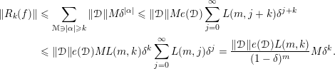 $$\begin{eqnarray}\displaystyle \Vert R_{k}(f)\Vert & {\leqslant} & \displaystyle \mathop{\sum }_{{\mathcal{M}}\ni |\unicode[STIX]{x1D6FC}|\geqslant k}\Vert {\mathcal{D}}\Vert M\unicode[STIX]{x1D6FF}^{|\unicode[STIX]{x1D6FC}|}\leqslant \Vert {\mathcal{D}}\Vert Me({\mathcal{D}})\mathop{\sum }_{j=0}^{\infty }L(m,j+k)\unicode[STIX]{x1D6FF}^{j+k}\nonumber\\ \displaystyle & {\leqslant} & \displaystyle \Vert {\mathcal{D}}\Vert e({\mathcal{D}})ML(m,k)\unicode[STIX]{x1D6FF}^{k}\mathop{\sum }_{j=0}^{\infty }L(m,j)\unicode[STIX]{x1D6FF}^{j}=\frac{\Vert {\mathcal{D}}\Vert e({\mathcal{D}})L(m,k)}{(1-\unicode[STIX]{x1D6FF})^{m}}M\unicode[STIX]{x1D6FF}^{k}.\end{eqnarray}$$
◻
3.2 Interpolation determinants
Let $\mathbf{f}:=(f_{1},\ldots ,f_{\unicode[STIX]{x1D707}})$
be a collection of functions and
$\mathbf{f}:=(f_{1},\ldots ,f_{\unicode[STIX]{x1D707}})$
be a collection of functions and $\mathbf{p}:=(p_{1},\ldots ,p_{\unicode[STIX]{x1D707}})$
a collection of points. We define the interpolation determinant
$\mathbf{p}:=(p_{1},\ldots ,p_{\unicode[STIX]{x1D707}})$
a collection of points. We define the interpolation determinant
 $$\begin{eqnarray}\unicode[STIX]{x1D6E5}(\mathbf{f},\mathbf{p}):=\det (f_{i}(p_{j}))_{1\leqslant i,j\leqslant \unicode[STIX]{x1D707}}.\end{eqnarray}$$
In the asymptotic notation ${\sim}_{m},O_{m},\unicode[STIX]{x1D6FA}_{m}$
in the following we use the subscript
${\sim}_{m},O_{m},\unicode[STIX]{x1D6FA}_{m}$
in the following we use the subscript $m$
to indicate that the implied constants depend only on
$m$
to indicate that the implied constants depend only on $m$
. The following lemma and its proof are direct analogs of the interpolation determinant estimates of [Reference Bombieri and PilaBP89]. We remark that in this paper we will not make explicit use of the estimates for the constants
$m$
. The following lemma and its proof are direct analogs of the interpolation determinant estimates of [Reference Bombieri and PilaBP89]. We remark that in this paper we will not make explicit use of the estimates for the constants $C,E$
in terms of
$C,E$
in terms of $\Vert {\mathcal{D}}\Vert ,e({\mathcal{D}})$
.
$\Vert {\mathcal{D}}\Vert ,e({\mathcal{D}})$
.
Lemma 9. Assume $m>0$
. Suppose
$m>0$
. Suppose $f_{i}\in {\mathcal{O}}(\bar{\unicode[STIX]{x1D6E5}}^{\prime })$
with
$f_{i}\in {\mathcal{O}}(\bar{\unicode[STIX]{x1D6E5}}^{\prime })$
with $\Vert f_{i}\Vert _{\unicode[STIX]{x1D6E5}^{\prime }}\leqslant M$
and
$\Vert f_{i}\Vert _{\unicode[STIX]{x1D6E5}^{\prime }}\leqslant M$
and $p_{i}\in D\cap X$
for
$p_{i}\in D\cap X$
for $i=1,\ldots ,\unicode[STIX]{x1D707}$
. Assume
$i=1,\ldots ,\unicode[STIX]{x1D707}$
. Assume $\unicode[STIX]{x1D6FF}<1/2$
. Then
$\unicode[STIX]{x1D6FF}<1/2$
. Then
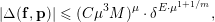 $$\begin{eqnarray}|\unicode[STIX]{x1D6E5}(\mathbf{f},\mathbf{p})|\leqslant (C\unicode[STIX]{x1D707}^{3}M)^{\unicode[STIX]{x1D707}}\cdot \unicode[STIX]{x1D6FF}^{E\cdot \unicode[STIX]{x1D707}^{1+1/m}},\end{eqnarray}$$
where
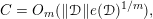 $$\begin{eqnarray}\displaystyle C & = & \displaystyle O_{m}(\Vert {\mathcal{D}}\Vert e({\mathcal{D}})^{1/m}),\end{eqnarray}$$
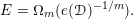 $$\begin{eqnarray}\displaystyle E & = & \displaystyle \unicode[STIX]{x1D6FA}_{m}(e({\mathcal{D}})^{-1/m}).\end{eqnarray}$$
Proof. We set
 $$\begin{eqnarray}k:=\max \biggl\{j:\mathop{\sum }_{l=0}^{j}e({\mathcal{D}})L(m,l)<\unicode[STIX]{x1D707}\biggr\}.\end{eqnarray}$$
Since $\sum _{l=0}^{j}L(m,l)=L(m+1,j)$
is a polynomial of degree
$\sum _{l=0}^{j}L(m,l)=L(m+1,j)$
is a polynomial of degree $m$
we have
$m$
we have $k{\sim}_{m}(\unicode[STIX]{x1D707}/e({\mathcal{D}}))^{1/m}$
.
$k{\sim}_{m}(\unicode[STIX]{x1D707}/e({\mathcal{D}}))^{1/m}$
.
We consider the expansions (35) for each $f_{i}$
with
$f_{i}$
with $k$
as above,
$k$
as above,
 $$\begin{eqnarray}f_{i}=\mathop{\sum }_{\unicode[STIX]{x1D6FC}\in {\mathcal{M}}^{{<}k}}m_{\unicode[STIX]{x1D6FC}}(f_{i})+R_{k}(f_{i})+Q_{i}.\end{eqnarray}$$
We note that $Q_{i}$
vanishes identically on
$Q_{i}$
vanishes identically on $X\cap \unicode[STIX]{x1D6E5}$
and, in particular, at every
$X\cap \unicode[STIX]{x1D6E5}$
and, in particular, at every $p_{j}$
. By the definition of
$p_{j}$
. By the definition of $k$
, the number of remaining terms in (45) does not exceed
$k$
, the number of remaining terms in (45) does not exceed $\unicode[STIX]{x1D707}$
. We expand
$\unicode[STIX]{x1D707}$
. We expand $\unicode[STIX]{x1D6E5}(\mathbf{f},\mathbf{p})$
by linearity with respect to each column. We thus obtain a sum of at most
$\unicode[STIX]{x1D6E5}(\mathbf{f},\mathbf{p})$
by linearity with respect to each column. We thus obtain a sum of at most $\unicode[STIX]{x1D707}^{\unicode[STIX]{x1D707}}$
interpolation determinants
$\unicode[STIX]{x1D707}^{\unicode[STIX]{x1D707}}$
interpolation determinants $\unicode[STIX]{x1D6E5}_{I}$
where each
$\unicode[STIX]{x1D6E5}_{I}$
where each $f_{i}$
is replaced by either a monomial term
$f_{i}$
is replaced by either a monomial term $m_{\unicode[STIX]{x1D6FC}}(f_{i})$
or a residue term
$m_{\unicode[STIX]{x1D6FC}}(f_{i})$
or a residue term $R_{k}(f_{i})$
. By (37) we have for
$R_{k}(f_{i})$
. By (37) we have for $i=1,\ldots ,\unicode[STIX]{x1D707}$
and for every
$i=1,\ldots ,\unicode[STIX]{x1D707}$
and for every $\unicode[STIX]{x1D6FC}\in {\mathcal{M}}^{{<}k}$
,
$\unicode[STIX]{x1D6FC}\in {\mathcal{M}}^{{<}k}$
,
 $$\begin{eqnarray}\begin{array}{@{}rcl@{}}\Vert m_{\unicode[STIX]{x1D6FC}}(f_{i})\Vert \ & {\leqslant}\ & C_{0}\unicode[STIX]{x1D6FF}^{|\unicode[STIX]{x1D6FC}|}\\ \Vert R_{k}(f_{i})\Vert \ & {\leqslant}\ & C_{0}\unicode[STIX]{x1D6FF}^{k}\end{array}\quad \text{where }C_{0}:=\frac{\Vert {\mathcal{D}}\Vert e({\mathcal{D}})L(m,k)}{(1-\unicode[STIX]{x1D6FF})^{m}}M.\end{eqnarray}$$
We remark that these are estimates for the maximum norm in $D$
and, in particular, they bound the absolute value of
$D$
and, in particular, they bound the absolute value of $m_{\unicode[STIX]{x1D6FC}}(f_{i}),R_{k}(f_{i})$
at every point
$m_{\unicode[STIX]{x1D6FC}}(f_{i}),R_{k}(f_{i})$
at every point $p_{j}$
.
$p_{j}$
.
Note that if the same index $\unicode[STIX]{x1D6FC}$
is repeated in two different columns of
$\unicode[STIX]{x1D6FC}$
is repeated in two different columns of $\unicode[STIX]{x1D6E5}_{I}$
, then these columns are linearly dependent and
$\unicode[STIX]{x1D6E5}_{I}$
, then these columns are linearly dependent and $\unicode[STIX]{x1D6E5}_{I}\equiv 0$
. Thus, for every non-zero
$\unicode[STIX]{x1D6E5}_{I}\equiv 0$
. Thus, for every non-zero $\unicode[STIX]{x1D6E5}_{I}$
we can have at most
$\unicode[STIX]{x1D6E5}_{I}$
we can have at most
 $$\begin{eqnarray}H_{{\mathcal{M}}}(j)-H_{{\mathcal{M}}}(j-1)\leqslant e({\mathcal{D}})L(m,j)\end{eqnarray}$$
monomial terms of order $|\unicode[STIX]{x1D6FC}|=j$
. We now expand
$|\unicode[STIX]{x1D6FC}|=j$
. We now expand $\unicode[STIX]{x1D6E5}_{I}$
by the Laplace expansion. By definition of
$\unicode[STIX]{x1D6E5}_{I}$
by the Laplace expansion. By definition of $k$
and by (46) we conclude that for each
$k$
and by (46) we conclude that for each $\unicode[STIX]{x1D6E5}_{I}$
we have
$\unicode[STIX]{x1D6E5}_{I}$
we have
 $$\begin{eqnarray}|\unicode[STIX]{x1D6E5}_{I}|\leqslant \unicode[STIX]{x1D707}!C_{0}^{\unicode[STIX]{x1D707}}\unicode[STIX]{x1D6FF}^{S},\quad S(m,k):=\mathop{\sum }_{l=0}^{k}e({\mathcal{D}})L(m,l)\cdot l.\end{eqnarray}$$
Since $L(m,l)\cdot l$
is a polynomial of degree
$L(m,l)\cdot l$
is a polynomial of degree $m$
in
$m$
in $l$
, we conclude that
$l$
, we conclude that $S(m,k){\sim}_{m}e({\mathcal{D}})k^{m+1}$
.
$S(m,k){\sim}_{m}e({\mathcal{D}})k^{m+1}$
.
Plugging in $k{\sim}_{m}(\unicode[STIX]{x1D707}/e({\mathcal{D}}))^{1/m}$
we have
$k{\sim}_{m}(\unicode[STIX]{x1D707}/e({\mathcal{D}}))^{1/m}$
we have
 $$\begin{eqnarray}\displaystyle & C_{0}=O_{m}(\Vert {\mathcal{D}}\Vert e({\mathcal{D}})^{1/m}\unicode[STIX]{x1D707}^{1-1/m}M), & \displaystyle\end{eqnarray}$$
 $$\begin{eqnarray}\displaystyle & S(m,k){\sim}_{m}e({\mathcal{D}})^{-1/m}\unicode[STIX]{x1D707}^{1+1/m}. & \displaystyle\end{eqnarray}$$
Summing over the (at most) $\unicode[STIX]{x1D707}^{\unicode[STIX]{x1D707}}$
determinants
$\unicode[STIX]{x1D707}^{\unicode[STIX]{x1D707}}$
determinants $\unicode[STIX]{x1D6E5}_{I}$
we obtain (41).◻
$\unicode[STIX]{x1D6E5}_{I}$
we obtain (41).◻
3.3 Polynomial interpolation determinants
Let $d\in \mathbb{N}$
and fix an integer
$d\in \mathbb{N}$
and fix an integer $m<\ell \leqslant n$
. Let
$m<\ell \leqslant n$
. Let $\unicode[STIX]{x1D707}$
denote the dimension of the space of polynomials of degree at most
$\unicode[STIX]{x1D707}$
denote the dimension of the space of polynomials of degree at most $d$
in
$d$
in $\ell$
variables,
$\ell$
variables, $\unicode[STIX]{x1D707}=L(\ell +1,d)$
. Let
$\unicode[STIX]{x1D707}=L(\ell +1,d)$
. Let $\mathbf{f}:=(f_{1},\ldots ,f_{\ell })$
be a collection of functions and
$\mathbf{f}:=(f_{1},\ldots ,f_{\ell })$
be a collection of functions and $\mathbf{p}:=(p_{1},\ldots ,p_{\unicode[STIX]{x1D707}})$
a collection of points. We define the polynomial interpolation determinant of degree
$\mathbf{p}:=(p_{1},\ldots ,p_{\unicode[STIX]{x1D707}})$
a collection of points. We define the polynomial interpolation determinant of degree $d$
to be
$d$
to be
 $$\begin{eqnarray}\unicode[STIX]{x1D6E5}^{d}(\mathbf{f},\mathbf{p}):=\unicode[STIX]{x1D6E5}(\mathbf{g},\mathbf{p}),\quad \mathbf{g}=(\mathbf{f}^{\unicode[STIX]{x1D6FC}}:\unicode[STIX]{x1D6FC}\in \mathbb{N}^{\ell },|\unicode[STIX]{x1D6FC}|\leqslant d).\end{eqnarray}$$
Note that $\unicode[STIX]{x1D6E5}^{d}(\mathbf{f},\mathbf{p})=0$
if and only if there exists a polynomial of degree at most
$\unicode[STIX]{x1D6E5}^{d}(\mathbf{f},\mathbf{p})=0$
if and only if there exists a polynomial of degree at most $d$
in
$d$
in $\ell$
variables vanishing at the points
$\ell$
variables vanishing at the points $\mathbf{f}(p_{1}),\ldots ,\mathbf{f}(p_{\unicode[STIX]{x1D707}})$
.
$\mathbf{f}(p_{1}),\ldots ,\mathbf{f}(p_{\unicode[STIX]{x1D707}})$
.
Lemma 10. Let $H\in \mathbb{N}$
and suppose that
$H\in \mathbb{N}$
and suppose that
 $$\begin{eqnarray}H(f_{i}(p_{j}))\leqslant H,\quad i=1,\ldots ,\ell ,~j=1,\ldots ,\unicode[STIX]{x1D707}.\end{eqnarray}$$
Then $\unicode[STIX]{x1D6E5}^{d}(\mathbf{f},\mathbf{p})$
either vanishes or satisfies
$\unicode[STIX]{x1D6E5}^{d}(\mathbf{f},\mathbf{p})$
either vanishes or satisfies
 $$\begin{eqnarray}|\unicode[STIX]{x1D6E5}^{d}(\mathbf{f},\mathbf{p})|\geqslant H^{-\ell \unicode[STIX]{x1D707}d}.\end{eqnarray}$$
Proof. Let $Q_{i,j}$
denote the denominator of
$Q_{i,j}$
denote the denominator of $f_{i}(p_{j})$
for
$f_{i}(p_{j})$
for $i=1,\ldots ,\ell$
and
$i=1,\ldots ,\ell$
and $j=1,\ldots ,\unicode[STIX]{x1D707}$
. By assumption
$j=1,\ldots ,\unicode[STIX]{x1D707}$
. By assumption $Q_{i,j}\leqslant H$
. The row corresponding to
$Q_{i,j}\leqslant H$
. The row corresponding to $p_{j}$
in
$p_{j}$
in $\unicode[STIX]{x1D6E5}^{d}(\mathbf{f},\mathbf{p})$
consists of rational numbers with common denominator dividing
$\unicode[STIX]{x1D6E5}^{d}(\mathbf{f},\mathbf{p})$
consists of rational numbers with common denominator dividing $Q_{j}:=\prod _{i}Q_{i,j}^{d}$
. Factoring out
$Q_{j}:=\prod _{i}Q_{i,j}^{d}$
. Factoring out $Q_{j}$
from each row we obtain a matrix with integer entries, whose determinant is either vanishing or at least one in absolute value. In the non-vanishing case we have
$Q_{j}$
from each row we obtain a matrix with integer entries, whose determinant is either vanishing or at least one in absolute value. In the non-vanishing case we have
 $$\begin{eqnarray}|\unicode[STIX]{x1D6E5}^{d}(\mathbf{f},\mathbf{p})|\geqslant \mathop{\prod }_{j=1}^{\unicode[STIX]{x1D707}}Q_{j}^{-1}\geqslant H^{-\ell \unicode[STIX]{x1D707}d}.\end{eqnarray}$$
◻
Comparing Lemmas 9 and 10 we obtain the following.
Proposition 11. Let $M,H\geqslant 2$
, and suppose
$M,H\geqslant 2$
, and suppose $f_{i}\in {\mathcal{O}}(\bar{\unicode[STIX]{x1D6E5}}^{\prime })$
with
$f_{i}\in {\mathcal{O}}(\bar{\unicode[STIX]{x1D6E5}}^{\prime })$
with $\Vert f_{i}\Vert _{\unicode[STIX]{x1D6E5}^{\prime }}\leqslant M$
. Assume
$\Vert f_{i}\Vert _{\unicode[STIX]{x1D6E5}^{\prime }}\leqslant M$
. Assume $\unicode[STIX]{x1D6FF}<1/2$
. Let
$\unicode[STIX]{x1D6FF}<1/2$
. Let
 $$\begin{eqnarray}Y=\mathbf{f}(X\cap D)\subset \mathbb{C}^{\ell }.\end{eqnarray}$$
There exist a constant $C_{1}>0$
depending only on
$C_{1}>0$
depending only on $\ell$
such that if
$\ell$
such that if
 $$\begin{eqnarray}-\!\log \unicode[STIX]{x1D6FF}>C_{1}\frac{d^{-1}\log (\Vert {\mathcal{D}}\Vert e({\mathcal{D}}))+\log M+\log H}{(d^{\ell -m}/e({\mathcal{D}}))^{1/m}},\end{eqnarray}$$
then $Y(\mathbb{Q},H)$
is contained in an algebraic hypersurface of degree at most
$Y(\mathbb{Q},H)$
is contained in an algebraic hypersurface of degree at most $d$
in
$d$
in $\mathbb{C}^{\ell }$
. The same conclusion holds for
$\mathbb{C}^{\ell }$
. The same conclusion holds for $m=0$
if instead of (56) we assume
$m=0$
if instead of (56) we assume $d\geqslant e({\mathcal{D}})$
.
$d\geqslant e({\mathcal{D}})$
.
Proof. We consider first the case $m=0$
. In this case according to Example 5 the number of points in
$m=0$
. In this case according to Example 5 the number of points in $X\cap \unicode[STIX]{x1D6E5}$
is bounded by
$X\cap \unicode[STIX]{x1D6E5}$
is bounded by $e({\mathcal{D}})$
. In particular, this bounds the number of points in
$e({\mathcal{D}})$
. In particular, this bounds the number of points in $Y$
, and all the more in
$Y$
, and all the more in $Y(\mathbb{Q},H)$
. Thus, the claim holds with any
$Y(\mathbb{Q},H)$
. Thus, the claim holds with any $d\geqslant e({\mathcal{D}})$
.
$d\geqslant e({\mathcal{D}})$
.
Now assume $m>0$
and suppose toward contradiction that
$m>0$
and suppose toward contradiction that $Y(\mathbb{Q},H)$
is not contained in an algebraic hypersurface of degree at most
$Y(\mathbb{Q},H)$
is not contained in an algebraic hypersurface of degree at most $d$
in
$d$
in $\mathbb{C}^{\ell }$
. Then by standard linear algebra it follows that there exist
$\mathbb{C}^{\ell }$
. Then by standard linear algebra it follows that there exist $\mathbf{p}=(p_{1},\ldots ,p_{\unicode[STIX]{x1D707}})$
with
$\mathbf{p}=(p_{1},\ldots ,p_{\unicode[STIX]{x1D707}})$
with $p_{1},\ldots ,p_{\unicode[STIX]{x1D707}}\in X\cap D$
such that
$p_{1},\ldots ,p_{\unicode[STIX]{x1D707}}\in X\cap D$
such that $\{\mathbf{f}(p_{j}):j=1,\ldots ,\unicode[STIX]{x1D707}\}$
is a subset of
$\{\mathbf{f}(p_{j}):j=1,\ldots ,\unicode[STIX]{x1D707}\}$
is a subset of $Y(\mathbb{Q},H)$
and does not lie on the zero locus of a non-zero polynomial of degree
$Y(\mathbb{Q},H)$
and does not lie on the zero locus of a non-zero polynomial of degree $d$
. Then
$d$
. Then $|\unicode[STIX]{x1D6E5}^{d}(\mathbf{f},\mathbf{p})|\neq 0$
, and from Lemmas 10 and 9 we have
$|\unicode[STIX]{x1D6E5}^{d}(\mathbf{f},\mathbf{p})|\neq 0$
, and from Lemmas 10 and 9 we have
 $$\begin{eqnarray}H^{-\ell \unicode[STIX]{x1D707}d}\leqslant |\unicode[STIX]{x1D6E5}^{d}(\mathbf{f},\mathbf{p})|\leqslant (C\unicode[STIX]{x1D707}^{3}M^{d})^{\unicode[STIX]{x1D707}}\cdot \unicode[STIX]{x1D6FF}^{E\cdot \unicode[STIX]{x1D707}^{1+1/m}}.\end{eqnarray}$$
Takings logarithms and using $\unicode[STIX]{x1D707}{\sim}_{\ell }d^{\ell }$
we have
$\unicode[STIX]{x1D707}{\sim}_{\ell }d^{\ell }$
we have
 $$\begin{eqnarray}\displaystyle (d^{\ell }/e({\mathcal{D}}))^{1/m}\log \unicode[STIX]{x1D6FF}\geqslant -\unicode[STIX]{x1D6FA}_{\ell }(\log \Vert {\mathcal{D}}\Vert +m^{-1}\log e({\mathcal{D}})+3\ell \log d+d\log M+\ell d\log H). & & \displaystyle\end{eqnarray}$$
Noting that
 $$\begin{eqnarray}\frac{\log d}{d^{\ell /m}}=O_{\ell }(1)\end{eqnarray}$$
and collecting all asymptotic constants into $C_{1}$
we arrive at a contradiction with (56).◻
$C_{1}$
we arrive at a contradiction with (56).◻
Corollary 12. Let $\ell =m+1$
and suppose
$\ell =m+1$
and suppose $f_{i}\in {\mathcal{O}}(\bar{\unicode[STIX]{x1D6E5}}^{\prime })$
with
$f_{i}\in {\mathcal{O}}(\bar{\unicode[STIX]{x1D6E5}}^{\prime })$
with $\Vert f_{i}\Vert _{\unicode[STIX]{x1D6E5}^{\prime }}\leqslant M$
. Let
$\Vert f_{i}\Vert _{\unicode[STIX]{x1D6E5}^{\prime }}\leqslant M$
. Let
 $$\begin{eqnarray}Y=\mathbf{f}(X\cap D)\subset \mathbb{C}^{m+1}.\end{eqnarray}$$
For every $\unicode[STIX]{x1D700}>0$
there exist two positive constants
$\unicode[STIX]{x1D700}>0$
there exist two positive constants
 $$\begin{eqnarray}\displaystyle d & = & \displaystyle d(m,\unicode[STIX]{x1D700},e({\mathcal{D}})),\end{eqnarray}$$
 $$\begin{eqnarray}\displaystyle C & = & \displaystyle C(m,\unicode[STIX]{x1D700},e({\mathcal{D}}),\Vert {\mathcal{D}}\Vert ,M)\end{eqnarray}$$
such that if $\unicode[STIX]{x1D6FF}\leqslant CH^{-\unicode[STIX]{x1D700}}$
, then
$\unicode[STIX]{x1D6FF}\leqslant CH^{-\unicode[STIX]{x1D700}}$
, then $Y(\mathbb{Q},H)$
is contained in an algebraic hypersurface of degree at most
$Y(\mathbb{Q},H)$
is contained in an algebraic hypersurface of degree at most $d$
in
$d$
in $\mathbb{C}^{m+1}$
.
$\mathbb{C}^{m+1}$
.
Proof. By Proposition 11 for $m>0$
it is enough to choose
$m>0$
it is enough to choose
 $$\begin{eqnarray}\displaystyle & \unicode[STIX]{x1D700}>\frac{C_{1}}{(d/e({\mathcal{D}}))^{1/m}}, & \displaystyle\end{eqnarray}$$
 $$\begin{eqnarray}\displaystyle & -\!\log C>\frac{C_{1}d^{-1}\log (\Vert {\mathcal{D}}\Vert e({\mathcal{D}})M)}{(d/e({\mathcal{D}}))^{1/m}}, & \displaystyle\end{eqnarray}$$
and for $m=0$
it is enough to choose
$m=0$
it is enough to choose $d=e({\mathcal{D}})$
and, e.g.,
$d=e({\mathcal{D}})$
and, e.g., $C=1$
.◻
$C=1$
.◻
Pursuing a different asymptotic direction for the parameters we also obtain the following corollary.
Corollary 13. Suppose $m>0$
and
$m>0$
and $f_{i}\in {\mathcal{O}}(\bar{\unicode[STIX]{x1D6E5}}^{\prime })$
with
$f_{i}\in {\mathcal{O}}(\bar{\unicode[STIX]{x1D6E5}}^{\prime })$
with $\Vert f_{i}\Vert _{\unicode[STIX]{x1D6E5}^{\prime }}\leqslant M$
. Let
$\Vert f_{i}\Vert _{\unicode[STIX]{x1D6E5}^{\prime }}\leqslant M$
. Let
 $$\begin{eqnarray}Y=\mathbf{f}(X\cap D)\subset \mathbb{C}^{\ell }.\end{eqnarray}$$
There exists a constant
 $$\begin{eqnarray}C=C(\ell ,e({\mathcal{D}}),\Vert {\mathcal{D}}\Vert ,M)\end{eqnarray}$$
such that if $\unicode[STIX]{x1D6FF}<C$
, then there exists an algebraic hypersurface of degree at most
$\unicode[STIX]{x1D6FF}<C$
, then there exists an algebraic hypersurface of degree at most $(\log H)^{m/(\ell -m)}$
in
$(\log H)^{m/(\ell -m)}$
in $\mathbb{C}^{\ell }$
containing
$\mathbb{C}^{\ell }$
containing $Y(\mathbb{Q},H)$
.
$Y(\mathbb{Q},H)$
.
Proof. Choosing $d=(\log H)^{m/(\ell -m)}$
in Proposition 11 we see that the right-hand side of (56) is majorated by a constant depending only on
$d=(\log H)^{m/(\ell -m)}$
in Proposition 11 we see that the right-hand side of (56) is majorated by a constant depending only on $\ell ,e({\mathcal{D}}),\Vert {\mathcal{D}}\Vert ,M$
.◻
$\ell ,e({\mathcal{D}}),\Vert {\mathcal{D}}\Vert ,M$
.◻
We are now ready to finish the proof of Theorem 2.
Proof of Theorem 2.
By Theorem 3 applied to the family $K$
and the dimension
$K$
and the dimension $k$
, there exists a positive radius
$k$
, there exists a positive radius $r>0$
and constants
$r>0$
and constants $C_{D},C_{H}>0$
with the following property. For any
$C_{D},C_{H}>0$
with the following property. For any $v=(x,y)\in K$
there exists a decomposition datum
$v=(x,y)\in K$
there exists a decomposition datum ${\mathcal{D}}_{v}$
such that:
${\mathcal{D}}_{v}$
such that:
-
(1)
$\unicode[STIX]{x1D6E5}_{v}=\unicode[STIX]{x1D6E5}_{v}^{\prime }$
is centered at
$x$
, and
$B_{r}(x)\subset \unicode[STIX]{x1D6E5}_{v}$
; -
(2)
$\dim {\mathcal{M}}_{i}\leqslant k$
,
$\Vert {\mathcal{D}}\Vert _{v}\leqslant C_{D}$
and
$e({\mathcal{D}}_{v})\leqslant C_{H}$
; -
(3)
$X_{y}$
admits decomposition with respect to
${\mathcal{D}}$
.


Set $D_{v}:=\unicode[STIX]{x1D6E5}_{v}^{2/C}$
, where
$D_{v}:=\unicode[STIX]{x1D6E5}_{v}^{2/C}$
, where $C$
is the constant given in Corollary 13 with
$C$
is the constant given in Corollary 13 with $\ell =m$
and
$\ell =m$
and $\mathbf{f}$
given by the standard coordinates on
$\mathbf{f}$
given by the standard coordinates on $\mathbb{C}^{m}$
(note that
$\mathbb{C}^{m}$
(note that $C$
depends on
$C$
depends on $C_{D},C_{H}$
but not on
$C_{D},C_{H}$
but not on $v$
). Then by Corollary 13 we see that
$v$
). Then by Corollary 13 we see that $(X_{y}\cap D_{v})(\mathbb{Q},H)$
is contained in an algebraic hypersurface of degree
$(X_{y}\cap D_{v})(\mathbb{Q},H)$
is contained in an algebraic hypersurface of degree $(\log H)^{k/(m-k)}$
. It now remains to cover
$(\log H)^{k/(m-k)}$
. It now remains to cover $K$
by some finite number
$K$
by some finite number $C(K)$
of the discs
$C(K)$
of the discs $D_{v}$
and apply the above to each of them.◻
$D_{v}$
and apply the above to each of them.◻
4 Exploring rational points in admissible projections
We begin with a definition.
Definition 14. Let $X\subset \mathbb{C}^{m}$
and
$X\subset \mathbb{C}^{m}$
and $W\subset \mathbb{C}^{m}$
be two sets. We define
$W\subset \mathbb{C}^{m}$
be two sets. We define
 $$\begin{eqnarray}X(W):=\{w\in W:W_{w}\subset X\}\end{eqnarray}$$
to be the set of points of $W$
such that
$W$
such that $X$
contains the germ of
$X$
contains the germ of $W$
around
$W$
around $w$
, i.e. such that
$w$
, i.e. such that $w$
has a neighborhood
$w$
has a neighborhood $U_{w}\subset \mathbb{C}^{m}$
such that
$U_{w}\subset \mathbb{C}^{m}$
such that $W\cap U_{w}\subset X$
.
$W\cap U_{w}\subset X$
.
If $A\subset \mathbb{C}^{n}$
we denote by
$A\subset \mathbb{C}^{n}$
we denote by $A_{\mathbb{R}}:=A\cap \mathbb{R}^{n}$
. We remark that
$A_{\mathbb{R}}:=A\cap \mathbb{R}^{n}$
. We remark that
 $$\begin{eqnarray}(A(W))_{\mathbb{R}}\subset (A_{\mathbb{R}})(W_{\mathbb{R}}).\end{eqnarray}$$
We will consider Definition 14 in two cases: for $X\subset \mathbb{C}^{m}$
locally analytic and
$X\subset \mathbb{C}^{m}$
locally analytic and $W\subset \mathbb{C}^{m}$
an algebraic variety, and for
$W\subset \mathbb{C}^{m}$
an algebraic variety, and for $X\subset \mathbb{R}^{m}$
subanalytic and
$X\subset \mathbb{R}^{m}$
subanalytic and $W\subset \mathbb{R}^{m}$
a semi-algebraic set.
$W\subset \mathbb{R}^{m}$
a semi-algebraic set.
Our principal motivation for Definition 14 is the following direct consequence (cf. Theorem 6).
Lemma 15. Let $S\subset \mathbb{R}^{m}$
be a connected positive-dimensional semialgebraic set and
$S\subset \mathbb{R}^{m}$
be a connected positive-dimensional semialgebraic set and $A\subset \mathbb{R}^{m}$
. Then
$A\subset \mathbb{R}^{m}$
. Then $A(S)\subset A^{\text{alg}}$
.
$A(S)\subset A^{\text{alg}}$
.
We record some simple consequences.
Lemma 16. Let $A,B,W\subset \mathbb{C}^{m}$
. Then
$A,B,W\subset \mathbb{C}^{m}$
. Then
 $$\begin{eqnarray}A(W)\cup B(W)\subset (A\cup B)(W).\end{eqnarray}$$
If $A\subset B$
is relatively open, then
$A\subset B$
is relatively open, then
 $$\begin{eqnarray}B(W)\cap A=A(W).\end{eqnarray}$$
4.1 Projections from admissible graphs
Let $\unicode[STIX]{x1D6FA}_{z}\subset \mathbb{C}^{m},\unicode[STIX]{x1D6FA}_{w}\subset \mathbb{C}^{n}$
be domains and set
$\unicode[STIX]{x1D6FA}_{z}\subset \mathbb{C}^{m},\unicode[STIX]{x1D6FA}_{w}\subset \mathbb{C}^{n}$
be domains and set $\unicode[STIX]{x1D6FA}:=\unicode[STIX]{x1D6FA}_{z}\times \unicode[STIX]{x1D6FA}_{w}\subset \mathbb{C}^{m+n}$
. Let
$\unicode[STIX]{x1D6FA}:=\unicode[STIX]{x1D6FA}_{z}\times \unicode[STIX]{x1D6FA}_{w}\subset \mathbb{C}^{m+n}$
. Let $\unicode[STIX]{x1D6EC}$
be an analytic space. We denote by
$\unicode[STIX]{x1D6EC}$
be an analytic space. We denote by $\unicode[STIX]{x1D70B}_{z},\unicode[STIX]{x1D70B}_{w},\unicode[STIX]{x1D70B}_{\unicode[STIX]{x1D6EC}}$
the projections from
$\unicode[STIX]{x1D70B}_{z},\unicode[STIX]{x1D70B}_{w},\unicode[STIX]{x1D70B}_{\unicode[STIX]{x1D6EC}}$
the projections from $\unicode[STIX]{x1D6FA}\times \unicode[STIX]{x1D6EC}$
to
$\unicode[STIX]{x1D6FA}\times \unicode[STIX]{x1D6EC}$
to $\unicode[STIX]{x1D6FA}_{z},\unicode[STIX]{x1D6FA}_{w},\unicode[STIX]{x1D6EC}$
, respectively. We denote by
$\unicode[STIX]{x1D6FA}_{z},\unicode[STIX]{x1D6FA}_{w},\unicode[STIX]{x1D6EC}$
, respectively. We denote by $\unicode[STIX]{x1D70B}:\unicode[STIX]{x1D6FA}\times \unicode[STIX]{x1D6EC}\rightarrow \unicode[STIX]{x1D6FA}_{z}\times \unicode[STIX]{x1D6EC}$
the projection
$\unicode[STIX]{x1D70B}:\unicode[STIX]{x1D6FA}\times \unicode[STIX]{x1D6EC}\rightarrow \unicode[STIX]{x1D6FA}_{z}\times \unicode[STIX]{x1D6EC}$
the projection $\unicode[STIX]{x1D70B}=\unicode[STIX]{x1D70B}_{z}\times \unicode[STIX]{x1D70B}_{\unicode[STIX]{x1D6EC}}$
.
$\unicode[STIX]{x1D70B}=\unicode[STIX]{x1D70B}_{z}\times \unicode[STIX]{x1D70B}_{\unicode[STIX]{x1D6EC}}$
.
Let $U\subset \unicode[STIX]{x1D6FA}_{z}\times \unicode[STIX]{x1D6EC}$
be an open subset and
$U\subset \unicode[STIX]{x1D6FA}_{z}\times \unicode[STIX]{x1D6EC}$
be an open subset and $\unicode[STIX]{x1D713}:U\rightarrow \unicode[STIX]{x1D6FA}_{w}$
a function, and denote its graph by
$\unicode[STIX]{x1D713}:U\rightarrow \unicode[STIX]{x1D6FA}_{w}$
a function, and denote its graph by
 $$\begin{eqnarray}\unicode[STIX]{x1D6E4}_{\unicode[STIX]{x1D713}}:=\{(z,w,\unicode[STIX]{x1D706})\in \unicode[STIX]{x1D6FA}\times \unicode[STIX]{x1D6EC}:\unicode[STIX]{x1D713}(z,\unicode[STIX]{x1D706})=w\}.\end{eqnarray}$$
We denote by $\tilde{\unicode[STIX]{x1D713}}:U\rightarrow \unicode[STIX]{x1D6E4}_{\unicode[STIX]{x1D713}}$
the map
$\tilde{\unicode[STIX]{x1D713}}:U\rightarrow \unicode[STIX]{x1D6E4}_{\unicode[STIX]{x1D713}}$
the map $(z,\unicode[STIX]{x1D706})\rightarrow (z,\unicode[STIX]{x1D713}(z,\unicode[STIX]{x1D706}),\unicode[STIX]{x1D706})$
.
$(z,\unicode[STIX]{x1D706})\rightarrow (z,\unicode[STIX]{x1D713}(z,\unicode[STIX]{x1D706}),\unicode[STIX]{x1D706})$
.
Definition 17. We say that $\unicode[STIX]{x1D713}:U\,\rightarrow \,\unicode[STIX]{x1D6FA}_{w}$
is admissible if
$\unicode[STIX]{x1D713}:U\,\rightarrow \,\unicode[STIX]{x1D6FA}_{w}$
is admissible if $\unicode[STIX]{x1D6E4}\,=\,\unicode[STIX]{x1D6E4}_{\unicode[STIX]{x1D713}}$
is relatively compact in
$\unicode[STIX]{x1D6E4}\,=\,\unicode[STIX]{x1D6E4}_{\unicode[STIX]{x1D713}}$
is relatively compact in $\unicode[STIX]{x1D6FA}\times \unicode[STIX]{x1D6EC}$
, and if there exists an analytic subset
$\unicode[STIX]{x1D6FA}\times \unicode[STIX]{x1D6EC}$
, and if there exists an analytic subset $X_{\unicode[STIX]{x1D6E4}}\,\subset \,\unicode[STIX]{x1D6FA}\times \unicode[STIX]{x1D6EC}$
which agrees with
$X_{\unicode[STIX]{x1D6E4}}\,\subset \,\unicode[STIX]{x1D6FA}\times \unicode[STIX]{x1D6EC}$
which agrees with $\unicode[STIX]{x1D6E4}$
over
$\unicode[STIX]{x1D6E4}$
over $U$
, i.e.
$U$
, i.e. $X_{\unicode[STIX]{x1D6E4}}\,\cap \,\unicode[STIX]{x1D70B}^{-1}(U)=\unicode[STIX]{x1D6E4}$
.
$X_{\unicode[STIX]{x1D6E4}}\,\cap \,\unicode[STIX]{x1D70B}^{-1}(U)=\unicode[STIX]{x1D6E4}$
.
4.2 Rational points on admissible projections
For the remainder of this section we fix an admissible $\unicode[STIX]{x1D719}:U\rightarrow \unicode[STIX]{x1D6FA}_{w}$
. Our main result in this section is the following theorem.
$\unicode[STIX]{x1D719}:U\rightarrow \unicode[STIX]{x1D6FA}_{w}$
. Our main result in this section is the following theorem.
Theorem 4. Let $X\subset \unicode[STIX]{x1D6FA}\times \unicode[STIX]{x1D6EC}$
be an analytic family. Set
$X\subset \unicode[STIX]{x1D6FA}\times \unicode[STIX]{x1D6EC}$
be an analytic family. Set
 $$\begin{eqnarray}Y:=\unicode[STIX]{x1D70B}(X\cap \unicode[STIX]{x1D6E4})\subset \unicode[STIX]{x1D6FA}_{z}\times \unicode[STIX]{x1D6EC}.\end{eqnarray}$$
Let $\unicode[STIX]{x1D700}>0$
. There exist constants
$\unicode[STIX]{x1D700}>0$
. There exist constants $d=d(\unicode[STIX]{x1D6E4},\unicode[STIX]{x1D700})$
and
$d=d(\unicode[STIX]{x1D6E4},\unicode[STIX]{x1D700})$
and $N=N(\unicode[STIX]{x1D6E4},\unicode[STIX]{x1D700})$
with the following property. For any
$N=N(\unicode[STIX]{x1D6E4},\unicode[STIX]{x1D700})$
with the following property. For any $\unicode[STIX]{x1D706}\in \unicode[STIX]{x1D6EC}$
and any
$\unicode[STIX]{x1D706}\in \unicode[STIX]{x1D6EC}$
and any $H\in \mathbb{N}$
there exist at most
$H\in \mathbb{N}$
there exist at most $NH^{\unicode[STIX]{x1D700}}$
many irreducible algebraic varieties
$NH^{\unicode[STIX]{x1D700}}$
many irreducible algebraic varieties $V_{\unicode[STIX]{x1D6FC}}\subset \mathbb{C}^{m}$
with
$V_{\unicode[STIX]{x1D6FC}}\subset \mathbb{C}^{m}$
with $\deg V_{\unicode[STIX]{x1D6FC}}\leqslant d$
such that
$\deg V_{\unicode[STIX]{x1D6FC}}\leqslant d$
such that
 $$\begin{eqnarray}Y_{\unicode[STIX]{x1D706}}(\mathbb{Q},H)\subset \mathop{\bigcup }_{\unicode[STIX]{x1D6FC}}Y_{\unicode[STIX]{x1D706}}(V_{\unicode[STIX]{x1D6FC}}).\end{eqnarray}$$
We begin the proof of Theorem 4 with the following proposition.
Proposition 18. Let $X\subset \unicode[STIX]{x1D6FA}\times \unicode[STIX]{x1D6EC}$
be an analytic family and set
$X\subset \unicode[STIX]{x1D6FA}\times \unicode[STIX]{x1D6EC}$
be an analytic family and set
 $$\begin{eqnarray}Y:=\unicode[STIX]{x1D70B}(X\cap \unicode[STIX]{x1D6E4})\subset \unicode[STIX]{x1D6FA}_{z}\times \unicode[STIX]{x1D6EC}.\end{eqnarray}$$
Let $W\subset \mathbb{C}^{m}$
be an irreducible algebraic variety.
$W\subset \mathbb{C}^{m}$
be an irreducible algebraic variety.
Let $\unicode[STIX]{x1D700}>0$
. There exist constants
$\unicode[STIX]{x1D700}>0$
. There exist constants $d=d(\unicode[STIX]{x1D6E4},\unicode[STIX]{x1D700},\deg W)$
and
$d=d(\unicode[STIX]{x1D6E4},\unicode[STIX]{x1D700},\deg W)$
and $N=N(\unicode[STIX]{x1D6E4},\unicode[STIX]{x1D700},\deg W)$
with the following property. For any
$N=N(\unicode[STIX]{x1D6E4},\unicode[STIX]{x1D700},\deg W)$
with the following property. For any $\unicode[STIX]{x1D706}\in \unicode[STIX]{x1D6EC}$
and any
$\unicode[STIX]{x1D706}\in \unicode[STIX]{x1D6EC}$
and any $H\in \mathbb{N}$
there exist
$H\in \mathbb{N}$
there exist $NH^{\unicode[STIX]{x1D700}}$
hypersurfaces
$NH^{\unicode[STIX]{x1D700}}$
hypersurfaces $H_{\unicode[STIX]{x1D6FC}}\subset \mathbb{C}^{m}$
with
$H_{\unicode[STIX]{x1D6FC}}\subset \mathbb{C}^{m}$
with $\deg H_{\unicode[STIX]{x1D6FC}}\leqslant d$
such that
$\deg H_{\unicode[STIX]{x1D6FC}}\leqslant d$
such that $W\not \subset H_{\unicode[STIX]{x1D6FC}}$
and
$W\not \subset H_{\unicode[STIX]{x1D6FC}}$
and
 $$\begin{eqnarray}(Y_{\unicode[STIX]{x1D706}}\cap W)(\mathbb{Q},H)\subset Y_{\unicode[STIX]{x1D706}}(W)\cup \mathop{\bigcup }_{\unicode[STIX]{x1D6FC}}H_{\unicode[STIX]{x1D6FC}}.\end{eqnarray}$$
Proof. Since the statement involves only the intersection $X\cap \unicode[STIX]{x1D6E4}$
we may without loss of generality replace
$X\cap \unicode[STIX]{x1D6E4}$
we may without loss of generality replace $X$
by
$X$
by $X\cap X_{\unicode[STIX]{x1D6E4}}$
, and assume that
$X\cap X_{\unicode[STIX]{x1D6E4}}$
, and assume that $X\cap \unicode[STIX]{x1D70B}^{-1}(U)\subset \unicode[STIX]{x1D6E4}$
.
$X\cap \unicode[STIX]{x1D70B}^{-1}(U)\subset \unicode[STIX]{x1D6E4}$
.
Set $k:=\dim W$
. Let
$k:=\dim W$
. Let ${\mathcal{C}}$
denote the projective (hence, compact) Chow variety (see [Reference Gelfand, Kapranov and ZelevinskyGKZ94, Ch. 4]) parametrizing all effective algebraic cycles of dimension
${\mathcal{C}}$
denote the projective (hence, compact) Chow variety (see [Reference Gelfand, Kapranov and ZelevinskyGKZ94, Ch. 4]) parametrizing all effective algebraic cycles of dimension $k$
and degree equal to
$k$
and degree equal to $\deg W$
. We denote by
$\deg W$
. We denote by $R_{V}\in {\mathcal{C}}$
the point corresponding to a cycle
$R_{V}\in {\mathcal{C}}$
the point corresponding to a cycle $V$
. Then the following family is analytic,
$V$
. Then the following family is analytic,
 $$\begin{eqnarray}X^{\prime }\subset \unicode[STIX]{x1D6FA}\times (\unicode[STIX]{x1D6EC}\times {\mathcal{C}}),\quad X^{\prime }=\{(z,w,\unicode[STIX]{x1D706},R_{V}):(z,w,\unicode[STIX]{x1D706})\in X,z\in \operatorname{supp}V\}.\end{eqnarray}$$
Clearly,
 $$\begin{eqnarray}X_{(\unicode[STIX]{x1D706},{\mathcal{R}}_{W})}^{\prime }=X_{\unicode[STIX]{x1D706}}\cap (W\times \unicode[STIX]{x1D6FA}_{w}).\end{eqnarray}$$
We apply Theorem 3 to $X^{\prime }$
with the compact set
$X^{\prime }$
with the compact set $\bar{\unicode[STIX]{x1D6E4}}\times {\mathcal{C}}$
and consider the conclusion for points of the form
$\bar{\unicode[STIX]{x1D6E4}}\times {\mathcal{C}}$
and consider the conclusion for points of the form $(p,\unicode[STIX]{x1D706},R_{W})$
for
$(p,\unicode[STIX]{x1D706},R_{W})$
for $(p,\unicode[STIX]{x1D706})\in \bar{\unicode[STIX]{x1D6E4}}$
. We conclude that there exist
$(p,\unicode[STIX]{x1D706})\in \bar{\unicode[STIX]{x1D6E4}}$
. We conclude that there exist $r,C_{D},C_{H}>0$
depending only on
$r,C_{D},C_{H}>0$
depending only on $\unicode[STIX]{x1D6E4},\deg W$
such that for any
$\unicode[STIX]{x1D6E4},\deg W$
such that for any $(p,\unicode[STIX]{x1D706})\in \bar{\unicode[STIX]{x1D6E4}}$
there exists a decomposition datum
$(p,\unicode[STIX]{x1D706})\in \bar{\unicode[STIX]{x1D6E4}}$
there exists a decomposition datum ${\mathcal{D}}$
satisfying:
${\mathcal{D}}$
satisfying:
-
(1)
$\unicode[STIX]{x1D6E5}=\unicode[STIX]{x1D6E5}^{\prime }$
is centered at
$p$
, and
$B_{r}(p)\subset \unicode[STIX]{x1D6E5}\subset \unicode[STIX]{x1D6FA}$
; -
(2)
$\dim {\mathcal{M}}_{i}<k$
,
$\Vert {\mathcal{D}}\Vert \leqslant C_{D}$
and
$e({\mathcal{D}})\leqslant C_{H}$
; -
(3) the set
(78)admits decomposition with respect to
$$\begin{eqnarray}Z_{\unicode[STIX]{x1D706}}=(X_{\unicode[STIX]{x1D706}}\cap (W\times \unicode[STIX]{x1D6FA}_{w}))^{{<}k}\end{eqnarray}$$
${\mathcal{D}}$
.


Fix $\unicode[STIX]{x1D706}\in \unicode[STIX]{x1D6EC}$
, let
$\unicode[STIX]{x1D706}\in \unicode[STIX]{x1D6EC}$
, let $q\in Y_{\unicode[STIX]{x1D706}}\cap W$
, and suppose
$q\in Y_{\unicode[STIX]{x1D706}}\cap W$
, and suppose $q\not \in \operatorname{Sing}W$
and
$q\not \in \operatorname{Sing}W$
and $q\not \in Y_{\unicode[STIX]{x1D706}}(W)$
. Then the germ of
$q\not \in Y_{\unicode[STIX]{x1D706}}(W)$
. Then the germ of $W$
at
$W$
at $q$
is smooth
$q$
is smooth $k$
-dimensional and not contained in
$k$
-dimensional and not contained in $Y_{\unicode[STIX]{x1D706}}$
. Equivalently, its image
$Y_{\unicode[STIX]{x1D706}}$
. Equivalently, its image $\tilde{\unicode[STIX]{x1D713}}(W\times \{\unicode[STIX]{x1D706}\})\subset \unicode[STIX]{x1D6E4}$
is the germ of a smooth
$\tilde{\unicode[STIX]{x1D713}}(W\times \{\unicode[STIX]{x1D706}\})\subset \unicode[STIX]{x1D6E4}$
is the germ of a smooth $k$
-dimensional analytic set at
$k$
-dimensional analytic set at $\tilde{\unicode[STIX]{x1D713}}(q,\unicode[STIX]{x1D706})$
that is not contained in
$\tilde{\unicode[STIX]{x1D713}}(q,\unicode[STIX]{x1D706})$
that is not contained in $X_{\unicode[STIX]{x1D706}}$
. Since we assume
$X_{\unicode[STIX]{x1D706}}$
. Since we assume $X\subset \unicode[STIX]{x1D6E4}$
in a neighborhood of
$X\subset \unicode[STIX]{x1D6E4}$
in a neighborhood of $\tilde{\unicode[STIX]{x1D713}}(q,\unicode[STIX]{x1D706})$
, we conclude that the dimension of
$\tilde{\unicode[STIX]{x1D713}}(q,\unicode[STIX]{x1D706})$
, we conclude that the dimension of
 $$\begin{eqnarray}X_{\unicode[STIX]{x1D706}}\cap (W\times \unicode[STIX]{x1D6FA}_{w})=X_{\unicode[STIX]{x1D706}}\cap \unicode[STIX]{x1D6E4}_{\unicode[STIX]{x1D706}}\cap (W\times \unicode[STIX]{x1D6FA}_{w})=X_{\unicode[STIX]{x1D706}}\cap \tilde{\unicode[STIX]{x1D713}}(W\times \{\unicode[STIX]{x1D706}\})\end{eqnarray}$$
at $\tilde{\unicode[STIX]{x1D713}}(q,\unicode[STIX]{x1D706})$
is strictly smaller than
$\tilde{\unicode[STIX]{x1D713}}(q,\unicode[STIX]{x1D706})$
is strictly smaller than $k$
, i.e.
$k$
, i.e. $(q,\unicode[STIX]{x1D713}(q,\unicode[STIX]{x1D706}))\in Z_{\unicode[STIX]{x1D706}}$
and, thus,
$(q,\unicode[STIX]{x1D713}(q,\unicode[STIX]{x1D706}))\in Z_{\unicode[STIX]{x1D706}}$
and, thus, $q\in \unicode[STIX]{x1D70B}(Z_{\unicode[STIX]{x1D706}})$
. In conclusion,
$q\in \unicode[STIX]{x1D70B}(Z_{\unicode[STIX]{x1D706}})$
. In conclusion,
 $$\begin{eqnarray}Y_{\unicode[STIX]{x1D706}}\cap W\subset Y_{\unicode[STIX]{x1D706}}(W)\cup \operatorname{Sing}W\cup \unicode[STIX]{x1D70B}(Z_{\unicode[STIX]{x1D706}}).\end{eqnarray}$$
Fix a hypersurface $H_{0}\subset \mathbb{C}^{m}$
containing
$H_{0}\subset \mathbb{C}^{m}$
containing $\operatorname{Sing}W$
and not containing
$\operatorname{Sing}W$
and not containing $W$
. It is clear that one can choose
$W$
. It is clear that one can choose $H_{0}$
of some degree
$H_{0}$
of some degree $d_{0}$
depending only on
$d_{0}$
depending only on $\deg W$
.
$\deg W$
.
Since $\dim W=k$
, one can choose a subset of
$\dim W=k$
, one can choose a subset of $k$
coordinates on
$k$
coordinates on $\mathbb{C}^{m}$
, say
$\mathbb{C}^{m}$
, say $\mathbf{f}=(z_{1},\ldots ,z_{k})$
, such that
$\mathbf{f}=(z_{1},\ldots ,z_{k})$
, such that $\mathbf{f}:W\rightarrow \mathbb{C}^{k}$
is dominant. In particular, no non-zero polynomial in the coordinates
$\mathbf{f}:W\rightarrow \mathbb{C}^{k}$
is dominant. In particular, no non-zero polynomial in the coordinates $\mathbf{f}$
vanishes on
$\mathbf{f}$
vanishes on $W$
. Since
$W$
. Since $\bar{\unicode[STIX]{x1D6E4}}$
is compact, the coordinates
$\bar{\unicode[STIX]{x1D6E4}}$
is compact, the coordinates $\mathbf{f}$
are certainly bounded (in absolute value) in the
$\mathbf{f}$
are certainly bounded (in absolute value) in the $r$
-neighborhood of
$r$
-neighborhood of $\bar{\unicode[STIX]{x1D6E4}}$
by some number
$\bar{\unicode[STIX]{x1D6E4}}$
by some number $M$
. Fix some
$M$
. Fix some $\unicode[STIX]{x1D700}^{\prime }>0$
whose value will be determined later, and let
$\unicode[STIX]{x1D700}^{\prime }>0$
whose value will be determined later, and let
 $$\begin{eqnarray}\displaystyle d & = & \displaystyle d(m,\unicode[STIX]{x1D700}^{\prime },C_{H}),\end{eqnarray}$$
 $$\begin{eqnarray}\displaystyle C & = & \displaystyle C(m,\unicode[STIX]{x1D700}^{\prime },C_{H},C_{D},M)\end{eqnarray}$$
be the two constants of Corollary 12.
Let $\unicode[STIX]{x1D6FF}=CH^{-\unicode[STIX]{x1D700}^{\prime }}$
. Let
$\unicode[STIX]{x1D6FF}=CH^{-\unicode[STIX]{x1D700}^{\prime }}$
. Let $p\in (\bar{\unicode[STIX]{x1D6E4}})_{\unicode[STIX]{x1D706}}$
and denote
$p\in (\bar{\unicode[STIX]{x1D6E4}})_{\unicode[STIX]{x1D706}}$
and denote $D_{p}=D_{\unicode[STIX]{x1D6FF}r}(p)\subset \unicode[STIX]{x1D6FA}$
. We apply Corollary 12 to
$D_{p}=D_{\unicode[STIX]{x1D6FF}r}(p)\subset \unicode[STIX]{x1D6FA}$
. We apply Corollary 12 to $\mathbf{f}$
and the set
$\mathbf{f}$
and the set $Z_{\unicode[STIX]{x1D706}}$
and conclude that there exists a polynomial
$Z_{\unicode[STIX]{x1D706}}$
and conclude that there exists a polynomial $P_{p}(\mathbf{f})$
of degree at most
$P_{p}(\mathbf{f})$
of degree at most $d$
such that
$d$
such that
 $$\begin{eqnarray}(\unicode[STIX]{x1D70B}_{z}(D_{p}\cap Z_{\unicode[STIX]{x1D706}}))(\mathbb{Q},H)\subset \{P_{p}=0\}.\end{eqnarray}$$
We let $H_{p}:=\{P_{p}=0\}\subset \mathbb{C}^{m}$
.
$H_{p}:=\{P_{p}=0\}\subset \mathbb{C}^{m}$
.
Finally, it remains to cover the compact set $(\bar{\unicode[STIX]{x1D6E4}})_{\unicode[STIX]{x1D706}}$
by the polydiscs
$(\bar{\unicode[STIX]{x1D6E4}})_{\unicode[STIX]{x1D706}}$
by the polydiscs $\{D_{p}:p\in S\}$
for some finite set
$\{D_{p}:p\in S\}$
for some finite set $S\subset (\bar{\unicode[STIX]{x1D6E4}})_{\unicode[STIX]{x1D706}}$
and take
$S\subset (\bar{\unicode[STIX]{x1D6E4}})_{\unicode[STIX]{x1D706}}$
and take
 $$\begin{eqnarray}\{H_{\unicode[STIX]{x1D6FC}}\}=\{H_{0}\}\cup \{H_{p}:p\in S\}.\end{eqnarray}$$
Then (80) and the choice of $H_{0},H_{p}$
gives
$H_{0},H_{p}$
gives
 $$\begin{eqnarray}(Y_{\unicode[STIX]{x1D706}}\cap W)(\mathbb{Q},H)\subset Y_{\unicode[STIX]{x1D706}}(W)\cup \mathop{\bigcup }_{\unicode[STIX]{x1D6FC}}H_{\unicode[STIX]{x1D6FC}}\end{eqnarray}$$
as claimed.
Since each $D_{p}$
has radius at least
$D_{p}$
has radius at least $CrH^{-\unicode[STIX]{x1D700}^{\prime }}$
and
$CrH^{-\unicode[STIX]{x1D700}^{\prime }}$
and $\bar{\unicode[STIX]{x1D6E4}}$
is compact, it is easy to see that one can choose a covering of size at most
$\bar{\unicode[STIX]{x1D6E4}}$
is compact, it is easy to see that one can choose a covering of size at most $NH^{\unicode[STIX]{x1D700}^{\prime }(n+m)}$
, where
$NH^{\unicode[STIX]{x1D700}^{\prime }(n+m)}$
, where $N=N(Cr,\unicode[STIX]{x1D6E4},\unicode[STIX]{x1D700}^{\prime })$
. Finally taking
$N=N(Cr,\unicode[STIX]{x1D6E4},\unicode[STIX]{x1D700}^{\prime })$
. Finally taking $\unicode[STIX]{x1D700}^{\prime }=\unicode[STIX]{x1D700}/(n+m)$
we obtain the statement of the proposition.◻
$\unicode[STIX]{x1D700}^{\prime }=\unicode[STIX]{x1D700}/(n+m)$
we obtain the statement of the proposition.◻
The following lemma gives an inductive proof of Theorem 4, which is obtained for the case $W=\mathbb{C}^{m}$
.
$W=\mathbb{C}^{m}$
.
Lemma 19. Let $X\subset \unicode[STIX]{x1D6FA}\times \unicode[STIX]{x1D6EC}$
be an analytic family and set
$X\subset \unicode[STIX]{x1D6FA}\times \unicode[STIX]{x1D6EC}$
be an analytic family and set
 $$\begin{eqnarray}Y:=\unicode[STIX]{x1D70B}(X\cap \unicode[STIX]{x1D6E4})\subset \unicode[STIX]{x1D6FA}_{z}\times \unicode[STIX]{x1D6EC}.\end{eqnarray}$$
Let $W\subset \mathbb{C}^{n}$
be an irreducible algebraic variety.
$W\subset \mathbb{C}^{n}$
be an irreducible algebraic variety.
Let $\unicode[STIX]{x1D700}>0$
. There exist constants
$\unicode[STIX]{x1D700}>0$
. There exist constants $d=d(\unicode[STIX]{x1D6E4},\unicode[STIX]{x1D700},\deg W)$
and
$d=d(\unicode[STIX]{x1D6E4},\unicode[STIX]{x1D700},\deg W)$
and $N=N(\unicode[STIX]{x1D6E4},\unicode[STIX]{x1D700},\deg W)$
with the following property. For any
$N=N(\unicode[STIX]{x1D6E4},\unicode[STIX]{x1D700},\deg W)$
with the following property. For any $\unicode[STIX]{x1D706}\in \unicode[STIX]{x1D6EC}$
and any
$\unicode[STIX]{x1D706}\in \unicode[STIX]{x1D6EC}$
and any $H\in \mathbb{N}$
, there exist at most
$H\in \mathbb{N}$
, there exist at most $NH^{\unicode[STIX]{x1D700}}$
many irreducible algebraic varieties
$NH^{\unicode[STIX]{x1D700}}$
many irreducible algebraic varieties $V_{\unicode[STIX]{x1D6FC}}\subset \mathbb{C}^{m}$
with
$V_{\unicode[STIX]{x1D6FC}}\subset \mathbb{C}^{m}$
with $\deg V_{\unicode[STIX]{x1D6FC}}\leqslant d$
such that
$\deg V_{\unicode[STIX]{x1D6FC}}\leqslant d$
such that
 $$\begin{eqnarray}(Y_{\unicode[STIX]{x1D706}}\cap W)(\mathbb{Q},H)\subset \mathop{\bigcup }_{\unicode[STIX]{x1D6FC}}Y_{\unicode[STIX]{x1D706}}(V_{\unicode[STIX]{x1D6FC}}).\end{eqnarray}$$
Proof. We proceed by induction on $\dim W$
. Apply Proposition 18 to obtain a family of at most
$\dim W$
. Apply Proposition 18 to obtain a family of at most $N^{\prime }H^{\unicode[STIX]{x1D700}/2}$
hypersurfaces
$N^{\prime }H^{\unicode[STIX]{x1D700}/2}$
hypersurfaces $\{H_{\unicode[STIX]{x1D6FC}^{\prime }}\}\subset \mathbb{C}^{m}$
of degree
$\{H_{\unicode[STIX]{x1D6FC}^{\prime }}\}\subset \mathbb{C}^{m}$
of degree $d^{\prime }$
. Let
$d^{\prime }$
. Let $\{W_{\unicode[STIX]{x1D6FC}}\}$
denote the union over
$\{W_{\unicode[STIX]{x1D6FC}}\}$
denote the union over $\unicode[STIX]{x1D6FC}^{\prime }$
of the sets of irreducible components of
$\unicode[STIX]{x1D6FC}^{\prime }$
of the sets of irreducible components of $W\cap H_{\unicode[STIX]{x1D6FC}^{\prime }}$
. Then
$W\cap H_{\unicode[STIX]{x1D6FC}^{\prime }}$
. Then
 $$\begin{eqnarray}\displaystyle \#\{W_{\unicode[STIX]{x1D6FC}}\}\leqslant d^{\prime }N^{\prime }H^{\unicode[STIX]{x1D700}/2},\quad \dim W_{\unicode[STIX]{x1D6FC}}=\dim W-1,\quad \deg W_{\unicode[STIX]{x1D6FC}}\leqslant d^{\prime }\cdot \deg W & & \displaystyle\end{eqnarray}$$
and
 $$\begin{eqnarray}(Y_{\unicode[STIX]{x1D706}}\cap W)(\mathbb{Q},H)\subset Y_{\unicode[STIX]{x1D706}}(W)\cup \mathop{\bigcup }_{\unicode[STIX]{x1D6FC}}W_{\unicode[STIX]{x1D6FC}}.\end{eqnarray}$$
Apply the inductive hypothesis to each $W_{\unicode[STIX]{x1D6FC}}$
to obtain collections
$W_{\unicode[STIX]{x1D6FC}}$
to obtain collections $W_{\unicode[STIX]{x1D6FC},\unicode[STIX]{x1D6FD}}$
, of size at most
$W_{\unicode[STIX]{x1D6FC},\unicode[STIX]{x1D6FD}}$
, of size at most $N^{\prime \prime }H^{\unicode[STIX]{x1D700}/2}$
for each
$N^{\prime \prime }H^{\unicode[STIX]{x1D700}/2}$
for each $\unicode[STIX]{x1D6FC}$
, such that
$\unicode[STIX]{x1D6FC}$
, such that
 $$\begin{eqnarray}(Y_{\unicode[STIX]{x1D706}}\cap W_{\unicode[STIX]{x1D6FC}})(\mathbb{Q},H)\subset \mathop{\bigcup }_{\unicode[STIX]{x1D6FD}}W_{\unicode[STIX]{x1D6FC},\unicode[STIX]{x1D6FD}}.\end{eqnarray}$$
Finally, we take $\{V_{\unicode[STIX]{x1D6FC}}\}$
to be the union of the sets
$\{V_{\unicode[STIX]{x1D6FC}}\}$
to be the union of the sets $\{W\}$
and
$\{W\}$
and $\{W_{\unicode[STIX]{x1D6FC},\unicode[STIX]{x1D6FD}}\}$
. The size of
$\{W_{\unicode[STIX]{x1D6FC},\unicode[STIX]{x1D6FD}}\}$
. The size of $\{V_{\unicode[STIX]{x1D6FC}}\}$
is bounded by
$\{V_{\unicode[STIX]{x1D6FC}}\}$
is bounded by $1+d^{\prime }N^{\prime }N^{\prime \prime }H^{\unicode[STIX]{x1D700}}$
as claimed and (87) is satisfied by (89) and (90).◻
$1+d^{\prime }N^{\prime }N^{\prime \prime }H^{\unicode[STIX]{x1D700}}$
as claimed and (87) is satisfied by (89) and (90).◻
5 Subanalytic sets and
$L_{\text{an}}^{D}$

Let $I=[-1,1]$
. For
$I=[-1,1]$
. For $m\geqslant 0$
we let
$m\geqslant 0$
we let $\mathbb{R}\{X_{1},\ldots ,X_{m}\}$
denote the ring of power series converging in a neighborhood of
$\mathbb{R}\{X_{1},\ldots ,X_{m}\}$
denote the ring of power series converging in a neighborhood of $I^{m}$
. To each
$I^{m}$
. To each $f\in \mathbb{R}\{X_{1},\ldots ,X_{m}\}$
we naturally associate the map
$f\in \mathbb{R}\{X_{1},\ldots ,X_{m}\}$
we naturally associate the map $f:I^{m}\rightarrow \mathbb{R}$
.
$f:I^{m}\rightarrow \mathbb{R}$
.
We recall the language $L_{\text{an}}^{D}$
of [Reference Denef and van den DriesDvdD88]. The language includes a countable set of variables
$L_{\text{an}}^{D}$
of [Reference Denef and van den DriesDvdD88]. The language includes a countable set of variables $\{X_{1},X_{2},\ldots \}$
, a relation symbol
$\{X_{1},X_{2},\ldots \}$
, a relation symbol ${<}$
, a binary operation symbol
${<}$
, a binary operation symbol $D$
, and an
$D$
, and an $m$
-ary operation symbol
$m$
-ary operation symbol $f$
for every
$f$
for every $f\in \mathbb{R}\{X_{1},\ldots ,X_{m}\}$
satisfying
$f\in \mathbb{R}\{X_{1},\ldots ,X_{m}\}$
satisfying $f(I^{m})\subset I$
. We view
$f(I^{m})\subset I$
. We view $I$
as an
$I$
as an $L_{\text{an}}^{D}$
-structure by interpreting
$L_{\text{an}}^{D}$
-structure by interpreting ${<}$
and
${<}$
and $f$
in the obvious way and interpreting
$f$
in the obvious way and interpreting $D$
as restricted division, namely
$D$
as restricted division, namely
 $$\begin{eqnarray}D(x,y)=\left\{\begin{array}{@{}ll@{}}x/y,\quad & |x|\leqslant |y|\text{and }y\neq 0,\\ 0,\quad & \text{otherwise.}\end{array}\right.\end{eqnarray}$$
We denote by $L_{\text{an}}$
the language obtained from
$L_{\text{an}}$
the language obtained from $L_{\text{an}}^{D}$
by omitting
$L_{\text{an}}^{D}$
by omitting $D$
.
$D$
.
For every $L_{\text{an}}^{D}$
-term
$L_{\text{an}}^{D}$
-term $t(X_{1},\ldots ,X_{m})$
we have an associated map
$t(X_{1},\ldots ,X_{m})$
we have an associated map $t:I^{m}\rightarrow I$
that we denote by
$t:I^{m}\rightarrow I$
that we denote by $x\rightarrow t(x)$
. If
$x\rightarrow t(x)$
. If $t$
is an
$t$
is an $L_{\text{an}}$
-term, then this map is real analytic in
$L_{\text{an}}$
-term, then this map is real analytic in $I^{m}$
.
$I^{m}$
.
For an $L_{\text{an}}^{D}$
-formula
$L_{\text{an}}^{D}$
-formula $\unicode[STIX]{x1D719}(X_{1},\ldots ,X_{m})$
we write
$\unicode[STIX]{x1D719}(X_{1},\ldots ,X_{m})$
we write $\unicode[STIX]{x1D719}(I^{m})$
for the set of points
$\unicode[STIX]{x1D719}(I^{m})$
for the set of points $x\in I^{m}$
satisfying
$x\in I^{m}$
satisfying $\unicode[STIX]{x1D719}$
. If
$\unicode[STIX]{x1D719}$
. If $A\subset I^{m}$
we write
$A\subset I^{m}$
we write $\unicode[STIX]{x1D719}(A):=\unicode[STIX]{x1D719}(I^{m})\cap A$
. We will use the following key result of [Reference Denef and van den DriesDvdD88].
$\unicode[STIX]{x1D719}(A):=\unicode[STIX]{x1D719}(I^{m})\cap A$
. We will use the following key result of [Reference Denef and van den DriesDvdD88].
Theorem 5. $I$
has elimination of quantifiers in
$I$
has elimination of quantifiers in $L_{\text{an}}^{D}$
. As a consequence, a set
$L_{\text{an}}^{D}$
. As a consequence, a set $A\subset I^{m}$
is subanalytic in
$A\subset I^{m}$
is subanalytic in $\mathbb{R}^{m}$
if and only if it is defined by a quantifier-free formula
$\mathbb{R}^{m}$
if and only if it is defined by a quantifier-free formula $\unicode[STIX]{x1D719}$
of
$\unicode[STIX]{x1D719}$
of $L_{\text{an}}^{D}$
.
$L_{\text{an}}^{D}$
.
5.1 Admissible formulas
Let $U\subset \mathring{I}^{m}$
be an open subset. We define the notion of an
$U\subset \mathring{I}^{m}$
be an open subset. We define the notion of an $L_{\text{an}}^{D}$
-term admissible in
$L_{\text{an}}^{D}$
-term admissible in $U$
by recursion as follows: a variable
$U$
by recursion as follows: a variable $X_{j}$
is always admissible in
$X_{j}$
is always admissible in $U$
; a term
$U$
; a term $f(t_{1},\ldots ,t_{m})$
is admissible in
$f(t_{1},\ldots ,t_{m})$
is admissible in $U$
if and only if the terms
$U$
if and only if the terms $t_{1},\ldots ,t_{m}$
are admissible in
$t_{1},\ldots ,t_{m}$
are admissible in $U$
; and a term
$U$
; and a term $D(t_{1},t_{2})$
is admissible in
$D(t_{1},t_{2})$
is admissible in $U$
if
$U$
if $t_{1},t_{2}$
are admissible in
$t_{1},t_{2}$
are admissible in $U$
and if
$U$
and if
 $$\begin{eqnarray}|t_{1}(x)|\leqslant |t_{2}(x)|\quad \text{and}\quad t_{2}(x)\neq 0\end{eqnarray}$$
for every $x\in U$
. An easy induction gives the following.
$x\in U$
. An easy induction gives the following.
Lemma 20. If $t$
is admissible in
$t$
is admissible in $U$
then the map
$U$
then the map $t:U\rightarrow I$
is real analytic.
$t:U\rightarrow I$
is real analytic.
We will say that an $L_{\text{an}}^{D}$
-formula
$L_{\text{an}}^{D}$
-formula $\unicode[STIX]{x1D719}$
is admissible in
$\unicode[STIX]{x1D719}$
is admissible in $U$
if all terms appearing in
$U$
if all terms appearing in $\unicode[STIX]{x1D719}$
are admissible in
$\unicode[STIX]{x1D719}$
are admissible in $U$
. Here and below, when speaking about ‘terms appearing in
$U$
. Here and below, when speaking about ‘terms appearing in $\unicode[STIX]{x1D719}$
’ we consider not only the top-level terms appearing in the relations, but also every sub-term appearing in the construction tree of each term. The following proposition shows that when considering definable subsets of
$\unicode[STIX]{x1D719}$
’ we consider not only the top-level terms appearing in the relations, but also every sub-term appearing in the construction tree of each term. The following proposition shows that when considering definable subsets of $I$
one can essentially reduce to admissible formulas.
$I$
one can essentially reduce to admissible formulas.
Proposition 21. Let $U\subset \mathring{I}^{m}$
be an open subset and
$U\subset \mathring{I}^{m}$
be an open subset and $\unicode[STIX]{x1D719}(X_{1},\ldots ,X_{m})$
a quantifier-free
$\unicode[STIX]{x1D719}(X_{1},\ldots ,X_{m})$
a quantifier-free $L_{\text{an}}^{D}$
-formula. There exist open subsets
$L_{\text{an}}^{D}$
-formula. There exist open subsets $U_{1},\ldots ,U_{k}\subset U$
and quantifier-free
$U_{1},\ldots ,U_{k}\subset U$
and quantifier-free $L_{\text{an}}^{D}$
-formulas
$L_{\text{an}}^{D}$
-formulas $\unicode[STIX]{x1D719}_{1},\ldots ,\unicode[STIX]{x1D719}_{k}$
such that
$\unicode[STIX]{x1D719}_{1},\ldots ,\unicode[STIX]{x1D719}_{k}$
such that $\unicode[STIX]{x1D719}_{j}$
is admissible in
$\unicode[STIX]{x1D719}_{j}$
is admissible in $U_{j}$
and
$U_{j}$
and
 $$\begin{eqnarray}\unicode[STIX]{x1D719}(U)=\mathop{\bigcup }_{j=1}^{k}\unicode[STIX]{x1D719}_{j}(U_{j}).\end{eqnarray}$$
Proof. We prove the claim by induction on the number $N$
of
$N$
of $U$
-inadmissible terms in
$U$
-inadmissible terms in $\unicode[STIX]{x1D719}$
. Clearly, if this number is zero we are done. Otherwise, let
$\unicode[STIX]{x1D719}$
. Clearly, if this number is zero we are done. Otherwise, let $t$
be some minimal
$t$
be some minimal $U$
-inadmissible term in
$U$
-inadmissible term in $\unicode[STIX]{x1D719}$
, i.e. such that all sub-terms appearing in
$\unicode[STIX]{x1D719}$
, i.e. such that all sub-terms appearing in $t$
are
$t$
are $U$
-admissible. Express
$U$
-admissible. Express $\unicode[STIX]{x1D719}$
in the form
$\unicode[STIX]{x1D719}$
in the form
 $$\begin{eqnarray}\unicode[STIX]{x1D719}(X_{1},\ldots ,X_{m})=\unicode[STIX]{x1D719}^{\prime }(X_{1},\ldots ,X_{m},t)\end{eqnarray}$$
for a quantifier-free $L_{\text{an}}^{D}$
-formula
$L_{\text{an}}^{D}$
-formula $\unicode[STIX]{x1D719}^{\prime }$
of
$\unicode[STIX]{x1D719}^{\prime }$
of $m+1$
free variables. By the definition of admissibility it is clear that
$m+1$
free variables. By the definition of admissibility it is clear that $t=D(t_{1},t_{2})$
, and by minimality
$t=D(t_{1},t_{2})$
, and by minimality $t_{1},t_{2}$
are admissible in
$t_{1},t_{2}$
are admissible in $U$
. We let
$U$
. We let
 $$\begin{eqnarray}\displaystyle \unicode[STIX]{x1D719}_{1}\equiv \unicode[STIX]{x1D719},\quad U_{1}=\{x\in U:|t_{1}(x)|<|t_{2}(x)|\} & & \displaystyle\end{eqnarray}$$
and
 $$\begin{eqnarray}\displaystyle \unicode[STIX]{x1D719}_{2} & = & \displaystyle (|t_{1}|=|t_{2}|)\wedge (t_{2}\neq 0)\wedge \unicode[STIX]{x1D719}^{\prime }(X_{1},\ldots ,X_{m},1),\end{eqnarray}$$
 $$\begin{eqnarray}\displaystyle \unicode[STIX]{x1D719}_{3} & = & \displaystyle (|t_{1}|>|t_{2}|\vee (t_{2}=0))\wedge \unicode[STIX]{x1D719}^{\prime }(X_{1},\ldots ,X_{m},0),\end{eqnarray}$$
with $U_{2}=U_{3}=U$
. Note that for readability we use the absolute value as a shorthand above, but it is clear that the relations can be expressed in terms of the unary minus operation corresponding to the function
$U_{2}=U_{3}=U$
. Note that for readability we use the absolute value as a shorthand above, but it is clear that the relations can be expressed in terms of the unary minus operation corresponding to the function $-:I\rightarrow I,x\rightarrow (-x)$
.
$-:I\rightarrow I,x\rightarrow (-x)$
.
Since $t_{1},t_{2}$
are admissible in
$t_{1},t_{2}$
are admissible in $U$
they define real analytic (in particular, continuous) functions there, and the relation defining
$U$
they define real analytic (in particular, continuous) functions there, and the relation defining $U_{1}$
is indeed open. Moreover, in
$U_{1}$
is indeed open. Moreover, in $U_{1}$
the term
$U_{1}$
the term $t$
is admissible by definition and, hence, the number of
$t$
is admissible by definition and, hence, the number of $U_{1}$
-inadmissible terms in
$U_{1}$
-inadmissible terms in $\unicode[STIX]{x1D719}_{1}$
is strictly smaller than
$\unicode[STIX]{x1D719}_{1}$
is strictly smaller than $N$
. Similarly, the new relations introduced in
$N$
. Similarly, the new relations introduced in $\unicode[STIX]{x1D719}_{2}$
(respectively,
$\unicode[STIX]{x1D719}_{2}$
(respectively, $\unicode[STIX]{x1D719}_{3}$
) are admissible in
$\unicode[STIX]{x1D719}_{3}$
) are admissible in $U$
, and since the inadmissible
$U$
, and since the inadmissible $t$
is replaced by the admissible term
$t$
is replaced by the admissible term $1$
(respectively,
$1$
(respectively, $0$
) the number of
$0$
) the number of $U_{2}$
(respectively,
$U_{2}$
(respectively, $U_{3}$
) inadmissible terms is strictly smaller than
$U_{3}$
) inadmissible terms is strictly smaller than $N$
. It is an easy exercise to check that
$N$
. It is an easy exercise to check that
 $$\begin{eqnarray}\unicode[STIX]{x1D719}(U)=\mathop{\bigcup }_{j=1}^{3}\unicode[STIX]{x1D719}_{j}(U_{j}).\end{eqnarray}$$
The proof is now concluded by applying the inductive hypothesis to each pair $\unicode[STIX]{x1D719}_{j},U_{j}$
for
$\unicode[STIX]{x1D719}_{j},U_{j}$
for $j=1,2,3$
.◻
$j=1,2,3$
.◻
5.2 Basic formulas and equations
We say that $\unicode[STIX]{x1D719}$
is a basic
$\unicode[STIX]{x1D719}$
is a basic $D$
-formula if it has the form
$D$
-formula if it has the form
 $$\begin{eqnarray}\biggl(\bigwedge _{j=1}^{k}t_{j}(X_{1},\ldots ,X_{m})=0\biggr)\wedge \biggl(\bigwedge _{j=1}^{k^{\prime }}s_{j}(X_{1},\ldots ,X_{m})>0\biggr),\end{eqnarray}$$
where $t_{j},s_{j}$
are
$t_{j},s_{j}$
are $L_{\text{an}}^{D}$
-terms. It is easy to check the following.
$L_{\text{an}}^{D}$
-terms. It is easy to check the following.
Lemma 22. Every quantifier-free $L_{\text{an}}^{D}$
-formula
$L_{\text{an}}^{D}$
-formula $\unicode[STIX]{x1D719}$
is equivalent in the structure
$\unicode[STIX]{x1D719}$
is equivalent in the structure $I$
to a finite disjunction of basic formulas. If
$I$
to a finite disjunction of basic formulas. If $\unicode[STIX]{x1D719}$
is
$\unicode[STIX]{x1D719}$
is $U$
-admissible, then so are the basic formulas in the disjunction.
$U$
-admissible, then so are the basic formulas in the disjunction.
We say that $\unicode[STIX]{x1D719}$
is a basic
$\unicode[STIX]{x1D719}$
is a basic $D$
-equation if
$D$
-equation if $k^{\prime }=0$
, i.e. if it involves only equalities. If
$k^{\prime }=0$
, i.e. if it involves only equalities. If $\unicode[STIX]{x1D719}$
is a basic
$\unicode[STIX]{x1D719}$
is a basic $D$
-formula, we denote by
$D$
-formula, we denote by $\tilde{\unicode[STIX]{x1D719}}$
the basic
$\tilde{\unicode[STIX]{x1D719}}$
the basic $D$
-equation obtained by removing all inequalities.
$D$
-equation obtained by removing all inequalities.
Let $\unicode[STIX]{x1D719}$
be a
$\unicode[STIX]{x1D719}$
be a $U$
-admissible basic
$U$
-admissible basic $D$
-formula for some
$D$
-formula for some $U\subset I^{m}$
. Then
$U\subset I^{m}$
. Then $\tilde{\unicode[STIX]{x1D719}}$
is
$\tilde{\unicode[STIX]{x1D719}}$
is $U$
-admissible as well. Moreover, since all the terms
$U$
-admissible as well. Moreover, since all the terms $s_{j}$
evaluate to continuous functions in
$s_{j}$
evaluate to continuous functions in $U$
, the strict inequalities of
$U$
, the strict inequalities of $\unicode[STIX]{x1D719}$
are open in
$\unicode[STIX]{x1D719}$
are open in $U$
and we have the following.
$U$
and we have the following.
Lemma 23. Suppose $\unicode[STIX]{x1D719}$
is
$\unicode[STIX]{x1D719}$
is $U$
-admissible basic
$U$
-admissible basic $D$
-formula. Then
$D$
-formula. Then $\unicode[STIX]{x1D719}(U)$
is relatively open in
$\unicode[STIX]{x1D719}(U)$
is relatively open in $\tilde{\unicode[STIX]{x1D719}}(U)$
.
$\tilde{\unicode[STIX]{x1D719}}(U)$
.
The set defined by an admissible $D$
-equation can be described in terms of admissible projections in the sense of § 4.1.
$D$
-equation can be described in terms of admissible projections in the sense of § 4.1.
Proposition 24. Let $U\subset \mathring{I}^{m+l}$
and
$U\subset \mathring{I}^{m+l}$
and $\unicode[STIX]{x1D719}$
be a
$\unicode[STIX]{x1D719}$
be a $U$
-admissible
$U$
-admissible $D$
-equation,
$D$
-equation,
 $$\begin{eqnarray}\unicode[STIX]{x1D719}=(t_{1}=0)\wedge \cdots \wedge (t_{k}=0).\end{eqnarray}$$
In the notation of § 4.1, there exist:
-
(1) complex domains
(101)with
$$\begin{eqnarray}\displaystyle \unicode[STIX]{x1D6FA}_{z}\subset \mathbb{C}^{m},\quad \unicode[STIX]{x1D6FA}_{w}\subset \mathbb{C}^{N},\quad \unicode[STIX]{x1D6EC}\subset \mathbb{C}^{l} & & \displaystyle\end{eqnarray}$$
$N\in \mathbb{N}$
and
$I^{m+l}\subset \unicode[STIX]{x1D6FA}_{z}\times \unicode[STIX]{x1D6EC}$
;
-
(2) an open complex neighborhood
$U\subset U_{\mathbb{C}}\subset \unicode[STIX]{x1D6FA}_{z}\times \unicode[STIX]{x1D6EC}$
; -
(3) an analytic map
$\unicode[STIX]{x1D713}:U_{\mathbb{C}}\rightarrow \unicode[STIX]{x1D6FA}_{w}$
; -
(4) an analytic set
$X\subset \unicode[STIX]{x1D6FA}\times \unicode[STIX]{x1D6EC}$
;


such that $\unicode[STIX]{x1D713}$
is admissible and
$\unicode[STIX]{x1D713}$
is admissible and $Y:=\unicode[STIX]{x1D70B}(X\cap \unicode[STIX]{x1D6E4}_{\unicode[STIX]{x1D713}})$
satisfies
$Y:=\unicode[STIX]{x1D70B}(X\cap \unicode[STIX]{x1D6E4}_{\unicode[STIX]{x1D713}})$
satisfies $Y_{\mathbb{R}}=\unicode[STIX]{x1D719}(U)$
.
$Y_{\mathbb{R}}=\unicode[STIX]{x1D719}(U)$
.
Proof. Let $\{s_{1},\ldots ,s_{N}\}$
denote all terms of the type
$\{s_{1},\ldots ,s_{N}\}$
denote all terms of the type $s_{j}=D(s_{j,1},s_{j,2})$
appearing in
$s_{j}=D(s_{j,1},s_{j,2})$
appearing in $\unicode[STIX]{x1D719}$
. For notational convenience we write
$\unicode[STIX]{x1D719}$
. For notational convenience we write $X=X_{1},\ldots ,X_{m+n}$
and
$X=X_{1},\ldots ,X_{m+n}$
and $W=W_{1},\ldots ,W_{N}$
for variables on
$W=W_{1},\ldots ,W_{N}$
for variables on $\mathbb{R}^{n+m}$
and
$\mathbb{R}^{n+m}$
and $\mathbb{R}^{N}$
.
$\mathbb{R}^{N}$
.
For every term $t(X)$
appearing in
$t(X)$
appearing in $\unicode[STIX]{x1D719}$
we define an
$\unicode[STIX]{x1D719}$
we define an $L_{\text{an}}$
term
$L_{\text{an}}$
term $t^{\prime }(X,W)$
by recursion as follows: if
$t^{\prime }(X,W)$
by recursion as follows: if $t$
is a variable, then
$t$
is a variable, then $t^{\prime }:=t$
; if
$t^{\prime }:=t$
; if $t=f(t_{1},\ldots ,t_{k})$
, then
$t=f(t_{1},\ldots ,t_{k})$
, then $t^{\prime }=f(t_{1}^{\prime },\ldots ,t_{k}^{\prime })$
; finally, if
$t^{\prime }=f(t_{1}^{\prime },\ldots ,t_{k}^{\prime })$
; finally, if $t=s_{j}$
, then
$t=s_{j}$
, then $t^{\prime }=W_{j}$
. As
$t^{\prime }=W_{j}$
. As $L_{\text{an}}$
-terms, every term
$L_{\text{an}}$
-terms, every term $t^{\prime }$
corresponds to a real-analytic function
$t^{\prime }$
corresponds to a real-analytic function $t^{\prime }:I^{m+N+n}\rightarrow I$
. We let
$t^{\prime }:I^{m+N+n}\rightarrow I$
. We let $\unicode[STIX]{x1D6FA}_{z}\times \unicode[STIX]{x1D6FA}_{w}\times \unicode[STIX]{x1D6EC}$
denote some complex neighborhood of
$\unicode[STIX]{x1D6FA}_{z}\times \unicode[STIX]{x1D6FA}_{w}\times \unicode[STIX]{x1D6EC}$
denote some complex neighborhood of $I^{m+N+n}$
to which every term
$I^{m+N+n}$
to which every term $t^{\prime }$
admits analytic continuation.
$t^{\prime }$
admits analytic continuation.
By Lemma 20, all terms appearing in $\unicode[STIX]{x1D719}$
evaluate to real analytic maps from
$\unicode[STIX]{x1D719}$
evaluate to real analytic maps from $U$
to
$U$
to $I$
. We define a map
$I$
. We define a map $\unicode[STIX]{x1D713}:U\rightarrow \unicode[STIX]{x1D6FA}_{w}$
by
$\unicode[STIX]{x1D713}:U\rightarrow \unicode[STIX]{x1D6FA}_{w}$
by
 $$\begin{eqnarray}\unicode[STIX]{x1D713}(x)=(s_{1}(x),\ldots ,s_{N}(x)).\end{eqnarray}$$
We note that $\unicode[STIX]{x1D713}(U)\subset I^{N}$
and, by definition of
$\unicode[STIX]{x1D713}(U)\subset I^{N}$
and, by definition of $U$
-admissibility, all the terms
$U$
-admissibility, all the terms $s_{j,2}$
evaluate to non-vanishing functions on
$s_{j,2}$
evaluate to non-vanishing functions on $U$
. Let
$U$
. Let $U_{w}$
be a relatively compact neighborhood of
$U_{w}$
be a relatively compact neighborhood of $I^{N}$
in
$I^{N}$
in $\unicode[STIX]{x1D6FA}_{w}$
. Then there exists a relatively compact open neighborhood
$\unicode[STIX]{x1D6FA}_{w}$
. Then there exists a relatively compact open neighborhood $U_{\mathbb{C}}\subset \unicode[STIX]{x1D6FA}_{z}\times \unicode[STIX]{x1D6EC}$
of
$U_{\mathbb{C}}\subset \unicode[STIX]{x1D6FA}_{z}\times \unicode[STIX]{x1D6EC}$
of $U$
such that:
$U$
such that:
-
(1)
$(U_{\mathbb{C}})_{\mathbb{R}}=U$
and
$\unicode[STIX]{x1D713}(U_{\mathbb{C}})\subset U_{w}$
; -
(2) all terms appearing in
$\unicode[STIX]{x1D719}$
admit analytic continuation to
$U_{\mathbb{C}}$
; -
(3) all the terms
$s_{j,2}$
evaluate to non-vanishing maps on
$U_{\mathbb{C}}$
.


Henceforth, we view $U_{\mathbb{C}}$
as the domain of
$U_{\mathbb{C}}$
as the domain of $\unicode[STIX]{x1D713}$
. The graph
$\unicode[STIX]{x1D713}$
. The graph $\unicode[STIX]{x1D6E4}=\unicode[STIX]{x1D6E4}_{\unicode[STIX]{x1D713}}$
is relatively compact in
$\unicode[STIX]{x1D6E4}=\unicode[STIX]{x1D6E4}_{\unicode[STIX]{x1D713}}$
is relatively compact in $\unicode[STIX]{x1D6FA}\times \unicode[STIX]{x1D6EC}$
, being contained in the product of the relatively compact sets
$\unicode[STIX]{x1D6FA}\times \unicode[STIX]{x1D6EC}$
, being contained in the product of the relatively compact sets $U_{\mathbb{C}}\subset \unicode[STIX]{x1D6FA}_{z}\times \unicode[STIX]{x1D6EC}$
and
$U_{\mathbb{C}}\subset \unicode[STIX]{x1D6FA}_{z}\times \unicode[STIX]{x1D6EC}$
and $U_{w}\subset \unicode[STIX]{x1D6FA}_{w}$
.
$U_{w}\subset \unicode[STIX]{x1D6FA}_{w}$
.
By construction of $t^{\prime }$
it is clear that
$t^{\prime }$
it is clear that
 $$\begin{eqnarray}t(z,\unicode[STIX]{x1D706})=t^{\prime }(z,\unicode[STIX]{x1D713}(z,\unicode[STIX]{x1D706}),\unicode[STIX]{x1D706})\quad \text{for }(t,\unicode[STIX]{x1D706})\in U_{\mathbb{ C}}.\end{eqnarray}$$
We define the analytic subset $X_{\unicode[STIX]{x1D6E4}}\subset \unicode[STIX]{x1D6FA}\times \unicode[STIX]{x1D6EC}$
by
$X_{\unicode[STIX]{x1D6E4}}\subset \unicode[STIX]{x1D6FA}\times \unicode[STIX]{x1D6EC}$
by
 $$\begin{eqnarray}X_{\unicode[STIX]{x1D6E4}}=\{s_{j,2}^{\prime }W_{j}=s_{j,1}^{\prime }:j=1,\ldots ,N\}.\end{eqnarray}$$
It is easy to check by induction that $X_{\unicode[STIX]{x1D6E4}}$
agrees with
$X_{\unicode[STIX]{x1D6E4}}$
agrees with $\unicode[STIX]{x1D6E4}$
over
$\unicode[STIX]{x1D6E4}$
over $U_{\mathbb{C}}$
(using (103) and the fact that
$U_{\mathbb{C}}$
(using (103) and the fact that $s_{j,2}$
evaluate to non-vanishing maps on
$s_{j,2}$
evaluate to non-vanishing maps on $U_{\mathbb{C}}$
).
$U_{\mathbb{C}}$
).
Finally, we define $X\subset \unicode[STIX]{x1D6FA}\times \unicode[STIX]{x1D6EC}$
by
$X\subset \unicode[STIX]{x1D6FA}\times \unicode[STIX]{x1D6EC}$
by
 $$\begin{eqnarray}X=\{t_{1}^{\prime }=\cdots =t_{k}^{\prime }=0\}\end{eqnarray}$$
and set $Y:=\unicode[STIX]{x1D70B}(X\cap \unicode[STIX]{x1D6E4})\subset \unicode[STIX]{x1D6FA}_{z}\times \unicode[STIX]{x1D6EC}$
. Then (103) at the points of
$Y:=\unicode[STIX]{x1D70B}(X\cap \unicode[STIX]{x1D6E4})\subset \unicode[STIX]{x1D6FA}_{z}\times \unicode[STIX]{x1D6EC}$
. Then (103) at the points of $U=(U_{\mathbb{C}})_{\mathbb{R}}$
gives
$U=(U_{\mathbb{C}})_{\mathbb{R}}$
gives $Y_{\mathbb{R}}=\unicode[STIX]{x1D719}(U)$
.◻
$Y_{\mathbb{R}}=\unicode[STIX]{x1D719}(U)$
.◻
5.3 Estimate for subanalytic sets
To state the general form of our main result we introduce the notion of complexity of a semi-algebraic set. We say that a semialgebraic set $S\subset \mathbb{R}^{m}$
has complexity
$S\subset \mathbb{R}^{m}$
has complexity $(m,s,d)$
if it defined by a semialgebraic formula involving
$(m,s,d)$
if it defined by a semialgebraic formula involving $s$
different relations
$s$
different relations $P_{j}>0$
or
$P_{j}>0$
or $P_{j}=0$
, where the polynomials
$P_{j}=0$
, where the polynomials $P_{j}$
have degrees bounded by
$P_{j}$
have degrees bounded by $d$
.
$d$
.
Theorem 6. Let $A\subset \mathbb{R}^{m+n}$
be a bounded subanalytic set and
$A\subset \mathbb{R}^{m+n}$
be a bounded subanalytic set and $\unicode[STIX]{x1D700}>0$
. There exist constants
$\unicode[STIX]{x1D700}>0$
. There exist constants $d=d(A,\unicode[STIX]{x1D700})$
and
$d=d(A,\unicode[STIX]{x1D700})$
and $N=N(A,\unicode[STIX]{x1D700})$
with the following property. For any
$N=N(A,\unicode[STIX]{x1D700})$
with the following property. For any $y\in I^{n}$
and any
$y\in I^{n}$
and any $H\in \mathbb{N}$
, there exist at most
$H\in \mathbb{N}$
, there exist at most $NH^{\unicode[STIX]{x1D700}}$
many smooth connected semialgebraic sets
$NH^{\unicode[STIX]{x1D700}}$
many smooth connected semialgebraic sets $S_{\unicode[STIX]{x1D6FC}}\subset \mathbb{C}^{m}$
with complexity
$S_{\unicode[STIX]{x1D6FC}}\subset \mathbb{C}^{m}$
with complexity $(m,d,d)$
such that
$(m,d,d)$
such that
 $$\begin{eqnarray}A_{y}(\mathbb{Q},H)\subset \mathop{\bigcup }_{\unicode[STIX]{x1D6FC}}A_{y}(S_{\unicode[STIX]{x1D6FC}}).\end{eqnarray}$$
Proof. Rescaling $A$
by a sufficiently large integer,
$A$
by a sufficiently large integer, $\tilde{A}:=(1/M)A$
we may assume that
$\tilde{A}:=(1/M)A$
we may assume that $\tilde{A}\subset \mathring{I}^{n+m}$
. This clearly does not affect the heights of points by more than a constant factor, and it will suffice to prove the claim for
$\tilde{A}\subset \mathring{I}^{n+m}$
. This clearly does not affect the heights of points by more than a constant factor, and it will suffice to prove the claim for $\tilde{A}$
and then rescale the varieties
$\tilde{A}$
and then rescale the varieties $\tilde{V}_{\unicode[STIX]{x1D6FC}}$
back to
$\tilde{V}_{\unicode[STIX]{x1D6FC}}$
back to $V_{\unicode[STIX]{x1D6FC}}:=MV_{\unicode[STIX]{x1D6FC}}$
. We thus assume without loss of generality that
$V_{\unicode[STIX]{x1D6FC}}:=MV_{\unicode[STIX]{x1D6FC}}$
. We thus assume without loss of generality that $A\subset \mathring{I}^{n+m}$
.
$A\subset \mathring{I}^{n+m}$
.
By Theorem 5 we may write $A=\unicode[STIX]{x1D719}(\mathring{I}^{m+n})$
for some quantifier-free
$A=\unicode[STIX]{x1D719}(\mathring{I}^{m+n})$
for some quantifier-free $L_{\text{an}}^{D}$
-formula
$L_{\text{an}}^{D}$
-formula $\unicode[STIX]{x1D719}$
. By Proposition 21 and Lemma 22 we may write
$\unicode[STIX]{x1D719}$
. By Proposition 21 and Lemma 22 we may write
 $$\begin{eqnarray}A=\mathop{\bigcup }_{j=1}^{k}\mathop{\bigcup }_{i=1}^{n_{j}}\unicode[STIX]{x1D719}_{ji}(U_{j}),\end{eqnarray}$$
where $\unicode[STIX]{x1D719}_{ji}$
is a
$\unicode[STIX]{x1D719}_{ji}$
is a $U_{j}$
-admissible basic
$U_{j}$
-admissible basic $D$
-formula. By the first part of Lemma 16 it is clear that it will suffice to prove the claim with
$D$
-formula. By the first part of Lemma 16 it is clear that it will suffice to prove the claim with $A$
replaced by each
$A$
replaced by each $\unicode[STIX]{x1D719}_{ij}(U_{j})$
. We thus assume without loss of generality that
$\unicode[STIX]{x1D719}_{ij}(U_{j})$
. We thus assume without loss of generality that $\unicode[STIX]{x1D719}$
is already a
$\unicode[STIX]{x1D719}$
is already a $U$
-admissible basic
$U$
-admissible basic $D$
-formula and prove the claim for
$D$
-formula and prove the claim for $A=\unicode[STIX]{x1D719}(U)$
.
$A=\unicode[STIX]{x1D719}(U)$
.
Recall that $\tilde{\unicode[STIX]{x1D719}}$
is a
$\tilde{\unicode[STIX]{x1D719}}$
is a $U$
-admissible
$U$
-admissible $D$
-equation. We write
$D$
-equation. We write $B=\tilde{\unicode[STIX]{x1D719}}(\mathring{I}^{m+n})$
. Applying Proposition 24 to
$B=\tilde{\unicode[STIX]{x1D719}}(\mathring{I}^{m+n})$
. Applying Proposition 24 to $\tilde{\unicode[STIX]{x1D719}}$
and using Theorem 4 we construct a locally analytic set
$\tilde{\unicode[STIX]{x1D719}}$
and using Theorem 4 we construct a locally analytic set $Y\subset \mathbb{C}^{m+n}$
such that
$Y\subset \mathbb{C}^{m+n}$
such that $Y_{\mathbb{R}}=B$
, and for any
$Y_{\mathbb{R}}=B$
, and for any $y\in I^{n}$
there exist at most
$y\in I^{n}$
there exist at most $N^{\prime }H^{\unicode[STIX]{x1D700}}$
many irreducible algebraic varieties
$N^{\prime }H^{\unicode[STIX]{x1D700}}$
many irreducible algebraic varieties $V_{\unicode[STIX]{x1D6FC}}\subset \mathbb{C}^{m}$
with
$V_{\unicode[STIX]{x1D6FC}}\subset \mathbb{C}^{m}$
with $\deg V_{\unicode[STIX]{x1D6FC}}\leqslant d^{\prime }$
such that
$\deg V_{\unicode[STIX]{x1D6FC}}\leqslant d^{\prime }$
such that
 $$\begin{eqnarray}Y_{y}(\mathbb{Q},H)\subset \mathop{\bigcup }_{\unicode[STIX]{x1D6FC}}Y_{y}(V_{\unicode[STIX]{x1D6FC}})\end{eqnarray}$$
with $d,N$
as in Theorem 4. By (68) and
$d,N$
as in Theorem 4. By (68) and $Y_{\mathbb{R}}=B$
we have
$Y_{\mathbb{R}}=B$
we have
 $$\begin{eqnarray}B_{y}(\mathbb{Q},H)\subset \mathop{\bigcup }_{\unicode[STIX]{x1D6FC}}B_{y}({\mathcal{V}}_{\unicode[STIX]{x1D6FC}}),\quad {\mathcal{V}}_{\unicode[STIX]{x1D6FC}}=(V_{\unicode[STIX]{x1D6FC}})_{\mathbb{R}}.\end{eqnarray}$$
Finally, we recall that $A$
is relatively open in
$A$
is relatively open in $B$
by Lemma 23. Then the same is true for the fiber
$B$
by Lemma 23. Then the same is true for the fiber $A_{y}\subset B_{y}$
, and
$A_{y}\subset B_{y}$
, and
 $$\begin{eqnarray}\displaystyle A_{y}(\mathbb{Q},H)\subset A_{y}\cap (B_{y}(\mathbb{Q},H))\subset A_{y}\cap \mathop{\bigcup }_{\unicode[STIX]{x1D6FC}}B_{y}({\mathcal{V}}_{\unicode[STIX]{x1D6FC}}) & = & \displaystyle \mathop{\bigcup }_{\unicode[STIX]{x1D6FC}}(A_{y}\cap B_{y}({\mathcal{V}}_{\unicode[STIX]{x1D6FC}}))\nonumber\\ \displaystyle & = & \displaystyle \mathop{\bigcup }_{\unicode[STIX]{x1D6FC}}A_{y}({\mathcal{V}}_{\unicode[STIX]{x1D6FC}})\end{eqnarray}$$
where the last equality is given by the second part of Lemma 16.
If we write each real-algebraic variety ${\mathcal{V}}_{\unicode[STIX]{x1D6FC}}$
as a union of smooth connected strata
${\mathcal{V}}_{\unicode[STIX]{x1D6FC}}$
as a union of smooth connected strata ${\mathcal{V}}_{\unicode[STIX]{x1D6FC}}=\bigcup _{j}S_{\unicode[STIX]{x1D6FC},j}$
, then we have
${\mathcal{V}}_{\unicode[STIX]{x1D6FC}}=\bigcup _{j}S_{\unicode[STIX]{x1D6FC},j}$
, then we have
 $$\begin{eqnarray}A_{y}(\mathbb{Q},H)\subset \mathop{\bigcup }_{\unicode[STIX]{x1D6FC}}A({\mathcal{V}}_{\unicode[STIX]{x1D6FC}})\subset \mathop{\bigcup }_{\unicode[STIX]{x1D6FC},j}A(S_{\unicode[STIX]{x1D6FC},j}).\end{eqnarray}$$
It remains to note that since $\deg V_{\unicode[STIX]{x1D6FC}}\leqslant d^{\prime }$
, the number and complexity of the strata
$\deg V_{\unicode[STIX]{x1D6FC}}\leqslant d^{\prime }$
, the number and complexity of the strata $S_{\unicode[STIX]{x1D6FC},j}$
is bounded by some number
$S_{\unicode[STIX]{x1D6FC},j}$
is bounded by some number $d$
depending only on
$d$
depending only on $d^{\prime }$
. This follows from general uniformity properties in the algebraic category, and, in fact, one may derive explicit (and polynomial in
$d^{\prime }$
. This follows from general uniformity properties in the algebraic category, and, in fact, one may derive explicit (and polynomial in $d^{\prime }$
) estimates for
$d^{\prime }$
) estimates for $d$
(for details see [Reference Binyamini and NovikovBN17, Proposition 37]). Taking
$d$
(for details see [Reference Binyamini and NovikovBN17, Proposition 37]). Taking $N=N^{\prime }d$
finishes the proof.◻
$N=N^{\prime }d$
finishes the proof.◻
We can now finish the proof of Theorem 1.
Proof of Theorem 1.
By Theorem 6, for any $y\in I^{n}$
and any
$y\in I^{n}$
and any $H\in \mathbb{N}$
there exist at most
$H\in \mathbb{N}$
there exist at most $NH^{\unicode[STIX]{x1D700}}$
many smooth connected semialgebraic sets
$NH^{\unicode[STIX]{x1D700}}$
many smooth connected semialgebraic sets $S_{\unicode[STIX]{x1D6FC}}\subset \mathbb{C}^{m}$
such that
$S_{\unicode[STIX]{x1D6FC}}\subset \mathbb{C}^{m}$
such that
 $$\begin{eqnarray}A_{y}(\mathbb{Q},H)\subset \mathop{\bigcup }_{\unicode[STIX]{x1D6FC}}A_{y}(S_{\unicode[STIX]{x1D6FC}}).\end{eqnarray}$$
By Lemma 15, for any positive dimensional $S_{\unicode[STIX]{x1D6FC}}$
we have
$S_{\unicode[STIX]{x1D6FC}}$
we have $A(S_{\unicode[STIX]{x1D6FC}})\subset A_{y}^{\text{alg}}$
. Thus
$A(S_{\unicode[STIX]{x1D6FC}})\subset A_{y}^{\text{alg}}$
. Thus $\#A_{y}^{\text{trans}}(\mathbb{Q},H)$
is bounded by the number of zero-dimensional strata, i.e. by
$\#A_{y}^{\text{trans}}(\mathbb{Q},H)$
is bounded by the number of zero-dimensional strata, i.e. by $NH^{\unicode[STIX]{x1D700}}$
.◻
$NH^{\unicode[STIX]{x1D700}}$
.◻
Acknowledgements
We wish to thank Yossi Yomdin and Pierre Milman for helpful discussions.
