2. Theory

In Horstmann et al. (Reference Horstmann, Herreman and Weier2020), we derived an analytic solution describing the linear motion of gravity–capillary interfacial waves in upright circular cylinders undergoing a constant circular orbital motion. The defined theoretical framework is shown in figure 1$(a)$. An ideal circular cylinder of radius $R$ contains two immiscible liquid layers (subscripts $i=1,2$) of heights $h_i$, kinematic viscosities $\nu _i$ and densities $\rho _i$. Under the constraint $\rho _1 < \rho _2$, both liquids stably stratify due to gravity, $\boldsymbol {g} = -g \boldsymbol {e}_z$, and form a liquid–liquid interface at the position $z = \eta (r,\varphi )$. The origin of the cylindrical coordinate system $O(r,\varphi ,z)$ is located in the centre of the interface $\eta$ and follows the tank motion. Interfacial tension $\gamma$ was incorporated to also describe the capillary wave regime. The interfacial contact line at the sidewall was assumed to move freely while maintaining a static contact angle of $90^{\circ }$ (no meniscus). This idealised boundary condition is only justified if the capillary length $\delta _c = \sqrt {\gamma /(\rho _2-\rho _1)g}$ is far smaller than the lateral dimensions of the vessel, which is safely satisfied by all liquid stratifications presented in this study, having a capillary length of approximately $2\ \textrm {mm}$; see Bond numbers in table 1. The entire vessel is oscillated horizontally with a constant angular frequency $\varOmega$ along a circular trajectory of diameter $d_s$.

Table 1. Experimental parameters and corresponding dimensionless groups of the two conducted sets of experiments.

Figure 1. $(a)$ Schematic illustration of the orbitally excited cylindrical tank and $(b)$ photograph of our experimental set-up. The cylinder of radius $R$ is filled with two immiscible liquids, $i=1,2$, of densities $\rho _i$, kinematic viscosities $\nu _i$ and layer heights $h_i$, which stably stratify due to gravity $\boldsymbol {g}$ and form a distinct liquid–liquid interface of interfacial tension $\gamma$ at the position $z = \eta (r,\varphi )$. The orbital shaking table prescribes ideal circular motions of diameter $d_s$ and constant angular frequency $\varOmega$ to the tank while maintaining a fixed orientation. A charge-coupled device (CCD) camera is mounted coaxially above the observation tank to allow direct image acquisition in the non-inertial frame of reference. A transparent random dot pattern placed just beneath the tank bottom, which is homogeneously illuminated from below by a light-emitting diode (LED) array, serves as the background.

Most concisely, this wave problem is governed by eight key dimensionless groups. In compliance with the free-surface sloshing theory by Reclari et al. (Reference Reclari, Dreyer, Tissot, Obreschkow, Wurm and Farhat2014), we have chosen the following set of dimensionless numbers:

(2.1a–f) \begin{gather} Fr = \frac{d_s \varOmega^{2}}{2g}, \quad E = \frac{d_s}{2R}, \quad Re_i = \frac{\varOmega R^{2}}{\nu_i}, \quad H_i = \frac{h_i}{R}, \\ Bo = \frac{(\rho_2-\rho_1)gR^{2}}{\gamma}, A = \frac{\rho_2 - \rho_1}{\rho_1 + \rho_2}. \end{gather}

Here, $Fr$ denotes the Froude number representing the forcing expressed by the ratio of inertial force and gravitational acceleration. The normalised shaking diameter $E$ can be interpreted as the eccentricity, while $Re_i$ are the fluid-dependent Reynolds numbers, here weighting the cylinder radius with the boundary layer thicknesses $\delta _i \sim \sqrt {\nu _i /\varOmega }$. The importance of gravitational forces compared to interfacial tension forces is specified by the Bond number $Bo$. Finally, $H_i$ denote the dimensionless aspect ratios and the Atwood number $A$ characterises the transition from interfacial waves (small $A$) to free-surface waves ($A \approx 1$).

By introducing the dimensionless variables $\tilde {r} = r/R$, $\tilde {z} = z/R$ and $\tilde {t} = \varOmega t$, we (Horstmann et al. Reference Horstmann, Herreman and Weier2020) expressed the linear solution for the dimensionless wave elevation $\eta (\tilde {r},\varphi ,\tilde {t})/R$ in the following form:

(2.2)\begin{align} \dfrac{\eta (\tilde{r},\varphi,\tilde{t})}{R} = & \sum_{n=1}^{\infty}\dfrac{2Fr}{\left(1 + \dfrac{\epsilon_{1n}^{2}}{Bo}\right)}\dfrac{\textrm{J}_1 (\epsilon_{1n}\tilde{r})}{(\epsilon_{1n}^{2}-1)\textrm{J}_1 (\epsilon_{1n})} \nonumber\\ &\times \left[\!\dfrac{\varGamma^{2}_{\omega_{1n}}}{\dfrac{\left(\varGamma^{2}_{\omega_{1n}}-1\right)^{2}}{\varLambda_{1n}} +\varLambda_{1n}}\sin(\tilde{t} - \varphi) + \dfrac{\varGamma^{2}_{\omega_{1n}}}{\left(\varGamma^{2}_{\omega_{1n}}-1\right) + \dfrac{\varLambda^{2}_{1n}}{\left(\varGamma^{2}_{\omega_{1n}}-1\right)}}\cos(\tilde{t} -\varphi)\!\right]\!. \end{align}

Here $\varGamma _{\omega _{1n}} := \omega _{1n}/\varOmega$ are the dimensionless frequency ratios and $\varLambda _{1n} :=2\lambda _{1n}/\varOmega$ are the damping ratios, both of which are specified in Appendix A. The values $\lambda _{1n}$ refer here to the two-layer viscous damping rates derived in Herreman et al. (Reference Herreman, Nore, Guermond, Cappanera, Weber and Horstmann2019, appendix D). Further, $\textrm {J}_1$ denotes the first-order Bessel function of the first kind and the $\epsilon _{1n}$ indicate the discrete wavenumbers, given as the $n$ roots of the first derivative of the first-order Bessel function, $\textrm {J}^{'}_{1} (\epsilon _{1n}) = 0$ (Abramowitz & Stegun Reference Abramowitz and Stegun1972). Physically, the integers $n$ specify the number of antinodal cycles (crest–trough pairs) appearing in the wave excited with the frequency $\varOmega = \omega _{1n}$.

Perhaps the most intriguing feature of solution (2.2) is the description of phase lags developing between the wave motion and the orbital motion of the shaking table, which emerge in the presence of damping. The phase lag $\Delta \varphi$, explicitly given by

(2.3)\begin{equation} \Delta \varphi (\tilde{r}) = \textrm{arctan} \left(\dfrac{\,\displaystyle\sum_{n=1}^{\infty}\dfrac{1}{\left(Bo + \epsilon_{1n}^{2}\right)}\dfrac{\textrm{J}_1 (\epsilon_{1n}\tilde{r})}{(\epsilon_{1n}^{2}-1)\textrm{J}_1 (\epsilon_{1n})}\dfrac{\varLambda_{1n}\varGamma^{2}_{\omega_{1n}}}{(\varGamma^{2}_{\omega_{1n}}-1)^{2} +\varLambda_{1n}^{2}}\,}{\,\displaystyle\sum_{n=1}^{\infty}\dfrac{1}{\left(Bo + \epsilon_{1n}^{2}\right)}\dfrac{\textrm{J}_1 (\epsilon_{1n}\tilde{r})}{(\epsilon_{1n}^{2}-1)\textrm{J}_1 (\epsilon_{1n})}\dfrac{\varGamma^{2}_{\omega_{1n}}(\varGamma^{2}_{\omega_{1n}}-1)}{(\varGamma^{2}_{\omega_{1n}}-1)^{2} + \varLambda^{2}_{1n}}\,}\right),\end{equation}

is an intricate function of the radial position $\tilde {r}$. As a consequence, the different antinodal cycles are subject to different phase shifts (with respect to the motion of the shaker), which are largely dictated by the damping ratios $\varLambda _{1n}$. Exactly this effect is responsible for the spiral pattern formation since this position-dependent shifting introduces a relative twisting between the individual crest–trough pairs (antinodal cycles), letting the waves appear as one-armed spirals in superposition.

This mechanism, which differs fundamentally from the nonlinear spiral pattern formation occurring in reaction–diffusion systems and excitable media, deserves further explanation. In order to arrive at a more lucid understanding, we can graphically examine how the wave modes are composed of the fundamental Fourier–Bessel modes in the solution (2.2). Let us consider, by way of example, the third wave mode developing at the frequency $\varOmega = \omega _{13} \Longleftrightarrow \varGamma _{\omega _{13}} = 1$. To be formally exact, we would have to calculate this wave by summing up an infinite number of Fourier–Bessel modes $n$ in (2.2). However, only the first few summands contribute significantly to the wave mode, since the terms $\varGamma _{\omega _{1n}} = 1$, which appear in the denominators, are small (and therefore significant) only if $n$ closely matches, in this example, the third eigenfrequency. It is well known that the first $n$ fundamental Fourier–Bessel modes essentially define the wave structure of waves excited by the $n$th eigenfrequency. Higher terms only add small details.

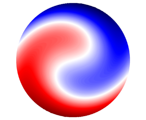
All this is illustrated in figure 2, showing the first three Fourier–Bessel modes, its superposition as well as the converged solution of a typical $\varOmega = \omega _{13}$ spiral wave pattern (compare to figure 2 in Horstmann et al. (Reference Horstmann, Herreman and Weier2020)) resulting from clockwise $(a)$ and anticlockwise $(b)$ circular excitation. It can be seen how the ongoing twisting of the fundamental modes leads to spiralisation. In the classic inviscid solution, all Fourier–Bessel modes have the same phase or are phase shifted by exactly $180^{\circ }$ such that the axial symmetry of the single modes is preserved in the superimposed solution. The presence of damping, in contrast, inevitably breaks this symmetry. A remarkable consequence of this symmetry breaking is that spiral waves are characterised by a pronounced chirality defined by the rotational direction of the shaking table. Clockwise and anticlockwise spiral waves are, unlike the classical solutions, no longer indistinguishable. The mere presence of a dissipation source allows the wave to ‘remember’ the rotational sense of excitation.

Figure 2. Spiral wave formation and origin of chirality highlighted by superimposing the first fundamental Fourier–Bessel modes for a clockwise-rotating orbit ($a$) and the anticlockwise-rotating orbit ($b$) of the third wave mode $\varOmega = \omega _{13}$ for the coherent spiral case shown in figure 3.

Expanding on this, we would like to discuss the spiral wave terminology in some more detail. Unfortunately, there is no consistent definition of spiral waves in the literature. Most generally, a spiral is described by a continuous monotonic function $r = r(\varphi )$ in polar coordinates. Such a relationship is evident from the white-coloured nodal ridges visible in the converged solution in figure 2, where the nodal radius is monotonically growing with the angle $\phi$. In terms of wave mechanics, however, we have to further distinguish between propagating and standing waves. Most spiral waves known, e.g. from reaction–diffusion systems, propagate either outwards from or inwards into the spiral centre (Vanag & Epstein Reference Vanag and Epstein2001). Such a radial propagation, also in contrast to vertically excited spiral Faraday waves (Kiyashko et al. Reference Kiyashko, Korzinov, Rabinovich and Tsimring1996), is not present in our solutions. Equation (2.2) describes a kind of standing wave that azimuthally rotates as a whole like a solid body with the fixed frequency predetermined by the shaking table. Please note, however, that nonlinear streaming effects arising at the sidewall will always cause a radial mean mass transport in the bulk, which is largely associated with the interface elevation (Bouvard et al. Reference Bouvard, Herreman and Moisy2017).

In Horstmann et al. (Reference Horstmann, Herreman and Weier2020), we have illustrated this spiral formation for different fixed damping rates in order to stress this phenomenon in a simple way. However, the formation of spiral waves turned out to be far more complex when applying the individual damping ratios $\varLambda _{1n}$ (A2), which can take considerably different values for the different wave modes $n$. Thereby, the wave crests and troughs do not necessarily merge into coherent spirals, but can become positionally separated and therefore incoherent. By way of examples, figure 3 shows different representative wave patterns that arise from solution (2.2). Essentially, we have identified four characteristic wave regimes: the well-known inviscid solutions, incoherent spirals with one or multiple discontinuities, continuous coherent spirals as well as overdamped waves, where the latter are defined by damping ratios larger than one $\varLambda _{\omega _{1n}} \geq 1$, due to which they would rapidly decay within only one wave period after switching off the shaking table.

Figure 3. Different characteristic spiral wave regimes visualised for the first three spiralisable modes appearing at the eigenfrequencies $\varOmega = \omega _{12}$, $\omega _{13}$ and $\omega _{14}$. The interface elevations $\eta (\tilde {r},\varphi )/\eta _0$, here normalised by the maximum wave amplitude $\eta _0$, are calculated by applying the default parameters $E=1$, $Bo = 10^{4}$, $A = 0.1$, $Re_1 = Re_2 = 12.5\times 10^{4} \sqrt {Fr}$, $H_1 = 2 - H_2$ and $H_2 = 0.8$ (incoherent spirals) in (2.2). The inviscid waves were created by taking the limits $Re_1 = Re_2 \gg 1$ and the overdamped waves by setting $Re_1 = Re_2 = 200 \sqrt {Fr}$. Finally, the coherent spirals are obtained by $H_2 = 0.05$. In each case, $Fr$ is chosen to correspond to the eigenfrequencies by setting $\varGamma _{\omega _{12}}$, $\varGamma _{\omega _{13}}$ and $\varGamma _{\omega _{14}} = 1$ in accordance with (A1). Black and green circles mark crest locations on the first nodal and antinodal cycle, respectively (see text).

This result has led to the question of if and how we can classify these regimes as functions of the dimensionless groups. As a first step, we seek a suitable wave criterion quantifying the degree of spiralisation. A simple way is the pair-by-pair comparison of the crest or trough amplitudes in the $j = 1,2,\ldots ,(n-1)$ nodal cycles (visible in the inviscid solutions as white rings), located at the positions

(2.4)\begin{align} \tilde{r}_{{ nodal},j} = \dfrac{\kappa_{1j}}{\left(\dfrac{\varGamma_{\omega_{1n+1}} - 1}{\varGamma_{\omega_{1n+1}} -\varGamma_{\omega_{1n}}}\right)\epsilon_{1n} + \left(\dfrac{1 -\varGamma_{\omega_{1n}}}{\varGamma_{\omega_{1n+1}} -\varGamma_{\omega_{1n}}}\right)\epsilon_{1n+1}}, \quad \textrm{for} \ \omega_{1n} \leq \varOmega < \omega_{1n+1}, \end{align}

with the ${\rm \pi} /2$ phase shifted inner amplitudes of the $j = 1,2,\ldots ,n$ antinodal cycles (crest–trough circles surrounding the white rings in the inviscid solution), located at the positions

(2.5)\begin{align} \tilde{r}_{{ antinodal},j} = \dfrac{\epsilon_{1j}}{\left(\dfrac{\varGamma_{\omega_{1n+1}} - 1}{\varGamma_{\omega_{1n+1}} -\varGamma_{\omega_{1n}}}\right)\epsilon_{1n} + \left(\dfrac{1 -\varGamma_{\omega_{1n}}}{\varGamma_{\omega_{1n+1}} -\varGamma_{\omega_{1n}}}\right)\epsilon_{1n+1}}, \quad \textrm{for} \ \omega_{1n} \leq \varOmega < \omega_{1n+1}. \end{align}

The numbers $\kappa _{1j}$ are given as the $j$ zeros of the first-order Bessel function $\textrm {J}_{1} (\kappa _{1j}) = 0$. In the case of resonant excitations ($\varOmega = \omega _{1n}$), expressions (2.4) and (2.5) simplify to $\tilde {r}_{{ nodal},j} = \kappa _{1j} / \epsilon _{1n}$ and $\tilde {r}_{{ antinodal},j} = \epsilon _{1j}/\epsilon _{1n}$.

For a better clarification, the points $\tilde {r}_{{ nodal},1}$ and $\tilde {r}_{{ antinodal},1}$ are marked as black and green dots, respectively, in the $\varOmega = \omega _{13}$ solutions in figure 3. In the case of inviscid waves, the pair-to-pair amplitude ratios at $\tilde {r}_{{ nodal},j}$ compared to $\tilde {r}_{{ antinodal},j}$ are always zero, whereas they would approach one for perfectly homogeneous spirals. On this basis, we introduce the spiralisation parameter $\mathcal {S}$ as follows:

(2.6)\begin{equation} \mathcal{S} := \min\left(\left|\dfrac{\eta (\tilde{r}=\tilde{r}_{{ nodal},j},\varphi = 0)}{\eta (\tilde{r}=\tilde{r}_{{ antinodal},j},\varphi = {\rm \pi}/2)} \right|\right), \quad j = 1,2,\ldots , (n-1) . \end{equation}

This parameter is suitable to analyse the spiralisation as a function of the dimensionless groups. Because spiral formation is a gradual process, there is no fixed threshold allowing one to distinguish sharply between coherent and incoherent spirals, but we observed numerically that spirals appear comparatively homogeneous and shaped like the coherent spirals presented in figure 3 for $\mathcal {S} > 0.1 \pm 0.02$. Therefore, we propose $\mathcal {S} \gtrsim 0.1$ as a criterion to identify coherent spirals, whereas the regime $\mathcal {S} \lesssim 0.1$ comprises incoherent spiral waves as well as the inviscid solutions $(\mathcal {S} = 0)$. Overdamped waves, in contrast, cannot be identified by means of the parameter since the inner nodal and antinodal cycles gradually disappear in this regime.

The numerical evaluation of $\mathcal {S}$ while varying all the dimensionless parameters (2.1a–f) revealed very complex spiralisation dynamics, with no obvious scaling dependences. Surprisingly, we found that the Reynolds numbers $Re_i$ are not the most critical parameters for achieving coherent spirals. The presence of damping is a necessary but not sufficient precondition. The Bond number $Bo$ and the aspect ratios $H_i$ have a more significant influence, with the general tendency that large $Bo$ (gravity wave limit) and shallow layers (either small $H_1$ or $H_2$) strongly favour coherent spirals. In contrast, $\mathcal {S}$ is independent of $E$ and depends only weakly on $A$ in the interfacial wave regime $A \lesssim 0.2$ considered here.

To provide a more quantitative understanding of the most important spiralisation characteristics, we study different parameter spaces around the accessible regimes of our experimental set-up introduced in § 3. In the following, we set $E = 1$ without loss of generality. Further, we choose $A=0.05$, a typical value for oil–water stratifications, assume symmetric viscosities $Re_1 = Re_2$ for the sake of simplicity and fix the aspect ratio of the cylinder to $H_1 + H_2 = 2$. Given these conditions, figure 4 shows the different spiral wave regimes in $H_2$–$Bo$ spaces for the first three spiralisable wave modes $\varOmega = \omega _{12}$, $\omega _{13}$ and $\omega _{14}$ and different damping strengths, here expressed in terms of the frequency-independent Galilei numbers $\sqrt {Ga_i} = Re_i /\sqrt {Fr} = \sqrt {gR^{3}\nu ^{2}_i}$. This reformulation was necessary to ensure comparability throughout the wave modes, which have very different eigenfrequencies. The three visualised spiral regimes represent different contour levels of $\mathcal {S}$, defined as follows: $\mathcal {S} < 0.08$ represents classic waves and incoherent spirals; $0.08 \leq \mathcal {S} \leq 0.12$ marks the transitional regime towards coherent spirals; and $\mathcal {S} > 0.12$ classifies clean coherent spirals. Although these boundaries were chosen somewhat arbitrarily on aesthetic grounds, figure 4 well reflects the overall spiralisation behaviour and reveals its complexity. The first presented mode $\varOmega = \omega _{12}$ plays a small role of its own, as the two nodal cycles merge particularly easily. All other modes (also higher modes not shown here) exhibit very similar but not identical behaviour: coherent spirals are predicted to evolve only for sufficiently high Galilei numbers in the gravity wave and shallow water limits.

Figure 4. Spiral regimes visualised in $H_2$–$Bo$ space for the wave modes $\varOmega = \omega _{12}$, $\omega _{13}$ and $\omega _{14}$ and different Galilei numbers $\sqrt {Ga_i} = Re_i /\sqrt {Fr} = \sqrt {gR^{3}\nu ^{2}}_i$. The Froude numbers were chosen to meet the eigenfrequencies $\varGamma _{\omega _{1n}} = 1$ according to (A1), with $E =1$, $A=0.05$ and $H_1 = 2 - H_2$. The coherent spiral regime is defined by $\mathcal {S} > 0.12$, whereas $\mathcal {S} < 0.08$ reflects incoherent spirals, including the classical inviscid solutions. In between, $0.08 \leq \mathcal {S} \leq 0.12$ highlights the gradual transition.

3. Experiment

In Horstmann et al. (Reference Horstmann, Wylega and Weier2019), we established an acoustic measurement technique for the reconstruction of rotating interfacial waves, originally with the aim of measuring waves in opaque liquid-metal stratifications. However, the proper verification of the smaller-scale spiral wave patterns requires continuous measurements to high resolution. For this purpose, we advanced the experimental apparatus to apply the background-oriented schlieren (BOS) method (often also called synthetic schlieren). This technique can be applied to directly measure the instantaneous topography of interfacial slopes between transparent fluids with different refractive indices (Moisy, Rabaud & Salsac Reference Moisy, Rabaud and Salsac2009). The implementation is shown in figure 1($b$). All experiments were conducted in a cylindrical vessel made from clean acrylic glass. The inner radius measures $R = 50\ \textrm {mm}$ and the total height of the inner volume was adjusted to $h_1 + h_2 = 75\ \textrm {mm}$. The entire observation cell is placed on a stand mounted on a $420\ \textrm {mm} \times 420\ \textrm {mm}$ shaking tray following ideal orbital motions excited by a modified Kuhner LS-X laboratory shaker. The shaker allows for a continuous adjustment of shaking diameters up to $d_s = 70\ \textrm {mm}$ and facilitates shaking frequencies $f = \varOmega /2 {\rm \pi}$ in the range $20\ \textrm {r.p.m.} \leq f \leq 500\ \textrm {r.p.m.}$

For the appropriate implementation of BOS, the experimental set-up from Horstmann et al. (Reference Horstmann, Wylega and Weier2019) was extended by two components. For backlight illumination, we have installed a Luminitronix MiniMatrix array of $10 \times 10$ LEDs ($15\ \textrm {cm} \times 15\ \textrm {cm}$) below the vessel. To achieve a homogeneous diffusive backlight, we further mounted a $2\ \textrm {mm}$ thick white sheet of polystyrene above the LED array. The emitted light passes vertically through the cylinder and is captured by an AVT Prosilica GT1660 monochrome camera. The camera was mounted coaxially $270\ \textrm {mm}$ above the vessel, resulting in an imaging of the fluid cell of $1000\ \textrm {px} \times 1000\ \textrm {px}$ with a resolution of $0.1\ \textrm {mm}~\textrm {px}^{-1}$. In this arrangement the camera follows the orbital motion of the shaking table, which has the advantage that acquired images can be processed directly without the need to transform the frame of reference. Finally, a transparent background was installed just beneath the bottom of the fluid vessel. We generated a random dot pattern of $\sim 20\ \textrm {dots}~\textrm {mm}^{-2}$ using the software PIVview that was printed onto a transparent plastic sheet.

The principle of BOS is based on the fact that local wave elevations are reflected as virtual displacements $\delta \boldsymbol {x} (r,\varphi )$ of the dot pattern with regard to a reference image obtained when the interface is flat. Light rays originating from points below the interface are refracted by a certain angle dependent on the local slope of the interface $\boldsymbol {\nabla }\eta (r,\varphi )$ and the refractive indices of all involved phases. For better clarification of this principle, a supplementary movie is provided (available at https://doi.org/10.1017/jfm.2021.686) showing spiral wave motion becoming directly visible as caustics in the reference pattern.

Our theoretical model predicts that coherent spirals preferentially form if one of the fluid layers is shallow. Fortunately, restricting to shallow bottom layers $H_2 \lesssim 0.25$ is also favourable for BOS measurements. It is shown by Moisy et al. (Reference Moisy, Rabaud and Salsac2009) that, if the reference pattern–interface distance is small and the camera–interface distance is large (paraxial approximation), the interfacial slope is linearly correlated with the displacement field,

(3.1)\begin{equation} \boldsymbol{\nabla}\eta (r,\varphi) \sim{-}\delta \boldsymbol{x} (r,\varphi), \end{equation}

provided that wave amplitudes and slopes are small $\lVert \eta _{1n}\rVert \ll R/\epsilon _{1n}$, which was anyway a basic requirement for the linearisation of our model (Horstmann et al. Reference Horstmann, Herreman and Weier2020). In principle, it is possible to determine the proportionality analytically by reconstructing the ray paths and inverting (3.1). This would allow one to determine wave amplitudes quantitatively, as recently demonstrated by Simonini et al. (Reference Simonini, Fontanarosa, De Giorgi and Vetrano2021) for free-surface sloshing in cylindrical containers. However, in our case the gradient is analytically known from (2.2). Therefore, we can avoid all the uncertainties that would arise from the reconstruction of the multiple refracted light rays and the numerical inversion procedure of (3.1).

In order to verify the predicted spiral patterns with the highest accuracy, it is expedient to directly compare normalised gradient fields $\boldsymbol {\nabla }\eta$ following from (2.2) with the experimental displacement fields $\delta \boldsymbol {x}$. This way, we compare the slope of the interface throughout space and time up to a single unknown scaling parameter, which is of no significance and can be eliminated through normalisation. Based on this concept, we determined $\delta \boldsymbol {x}$ from recorded schlieren patterns by correlating successive images using the software PIVview 3.6. All displacement fields presented below were phase-averaged and interpolated on a standardised $0.5\ \textrm {mm} \times 0.5\ \textrm {mm}$ Cartesian grid in order to increase the accuracy. This way, we could keep maximum measurement uncertainties in $\delta \boldsymbol {x} (r,\varphi )$ well below $\pm 0.1\ \textrm {mm}$.