


1. Introduction
The flow of an incompressible viscous fluid around an infinitely long circular cylinder is characterised by the Reynolds number,  ${\textit {Re}}=U_\infty d/\nu$ (defined by the free stream velocity $U_\infty$, the cylinder diameter $d$ and the kinematic viscosity $\nu$). With an increase of ${\textit {Re}}$, the flow undergoes several stages of stability loss before it becomes turbulent (Williamson Reference Williamson1996c). A key feature of the flow is the von Kármán vortex street which appears soon after the primary instability of the flow at ${\textit {Re}}={\textit {Re}}_{0}$ when the two-dimensional steady flow becomes time-periodic via supercritical Hopf bifurcation. Critical Reynolds numbers observed in experiments and obtained using theoretical analysis agree, ${\textit {Re}}_{0}\approx 46\unicode{x2013}47$ (Mathis, Provansal & Boyer Reference Mathis, Provansal and Boyer1984; Jackson Reference Jackson1987; Dušek, Le Gal & Fraunié Reference Dušek, Le Gal and Fraunié1994). This instability does not immediately lead to the appearance of the von Kármán vortex street – the formation of the vortices happens at a slightly larger Reynolds number far in the wake (approximately 100 diameters downstream) (Heil et al. Reference Heil, Rosso, Hazel and Brøns2017). As the Reynolds number is increased further, the two-dimensional time-periodic flow becomes unstable to two distinct modes (A and B) of three-dimensional instability (Barkley & Henderson Reference Barkley and Henderson1996), which are also observed experimentally (Williamson Reference Williamson1988). The modes have different spatio-temporal structure and length scale (approximately four and one diameter of the cylinder, respectively).
The mode A instability arises at a critical Reynolds number of  ${\textit {Re}}_A=188.5\pm 1$ and a wavelength of $\lambda _A=3.96\pm 0.02$ (Barkley & Henderson Reference Barkley and Henderson1996) via a subcritical bifurcation (Henderson & Barkley Reference Henderson and Barkley1996; Behara & Mittal Reference Behara and Mittal2010; Akbar, Bouchet & Dušek Reference Akbar, Bouchet and Dušek2011). These theoretical predictions agree with experiments, see discussions by Miller & Williamson (Reference Miller and Williamson1994), Williamson (Reference Williamson1996a), Akbar et al. (Reference Akbar, Bouchet and Dušek2011) and Jiang et al. (Reference Jiang, Cheng, Tong, Draper and An2016b). Barkley (Reference Barkley2005) demonstrated that the instability originates in the vortex formation region by applying a Floquet stability analysis to the various flow subregions. This showed that at ${\textit {Re}}=190$, the confined flow in the vortex formation region ( $0\le x\le 3$ and $|y|\le 1.5$) still exhibited a mode A instability (as manifested by the same dependence of the Floquet multiplier on the spanwise wavenumber as for the entire computational domain), whilst the developed wake (region $2.25\le x\le 25$ and $|y|\le 4$) turned out to be stable. This finding is supported by Giannetti, Camarri & Luchini (Reference Giannetti, Camarri and Luchini2010), who performed a sensitivity analysis of the dominant Floquet modes to localised structural perturbation and also provided time-resolved details of the most sensitive subregions of the flow.
A distinctive characteristic of mode A behind a circular cylinder is its degeneration into the neutral two-dimensional mode in the limit of infinite spanwise wavelength, as highlighted by Barkley & Henderson (Reference Barkley and Henderson1996). It is well known that, in general, periodic solutions  $\boldsymbol {U}(\boldsymbol {x},t)$ of autonomous problems admit neutrally stable Floquet modes in the form of $\partial \boldsymbol {U}(\boldsymbol {x},t)/\partial t$ (Iooss & Joseph Reference Iooss and Joseph1990, § VII.6.2). Therefore, given that mode A shares its symmetry with this two-dimensional neutral mode, it inherits the symmetry of the base flow $\boldsymbol {U}(\boldsymbol {x},t)$. Three-dimensional instabilities linked to such neutral modes also occur in other problems, and we show that this general mathematical fact has implications for the kinematics of long-wavelength three-dimensional instabilities, thus elucidating a perturbation pattern for a class of instabilities.
Mode A type instabilities are also observed in other flows, e.g. behind elongated bluff cylinders, oscillating cylinders, rotating cylinders, square and elliptic cylinders, airfoils, and behind cylinders moving near a wall (Ryan, Thompson & Hourigan Reference Ryan, Thompson and Hourigan2005; Leontini, Thompson & Hourigan Reference Leontini, Thompson and Hourigan2007; Luo, Tong & Khoo Reference Luo, Tong and Khoo2007; Sheard, Fitzgerald & Ryan Reference Sheard, Fitzgerald and Ryan2009; Lo Jacono et al. Reference Lo Jacono, Leontini, Thompson and Sheridan2010; Leontini, Lo Jacono & Thompson Reference Leontini, Lo Jacono and Thompson2015; Rao et al. Reference Rao, Radi, Leontini, Thompson, Sheridan and Hourigan2015; Agbaglah & Mavriplis Reference Agbaglah and Mavriplis2017; He et al. Reference He, Gioria, Pérez and Theofilis2017; Rao et al. Reference Rao, Leontini, Thompson and Hourigan2017; Thompson, Leweke & Hourigan Reference Thompson, Leweke and Hourigan2021). However, it is interesting to note that there is no universally accepted definition that allows one to classify a particular three-dimensional instability as being mode A. One possible way to do this is by constructing a continuous transformation between different problems and tracking the relevant solution branch; see, e.g. Leontini et al. (Reference Leontini, Lo Jacono and Thompson2015). A less rigorous but common approach is to compare what are thought to be ‘intrinsic’ attributes of the mode A pattern, such as its critical wavelength, the local distribution of the perturbations and the spatio-temporal symmetry of the perturbations. Yet, mode A type perturbations can emerge on the background of non-symmetric base flow, and their spanwise wavelength can be of the order of tens of diameters of the cylinder; see, e.g. the flow around an elliptic and rotating cylinder (Rao et al. Reference Rao, Radi, Leontini, Thompson, Sheridan and Hourigan2015, Reference Rao, Leontini, Thompson and Hourigan2017).
Over the years, many attempts have been made to explain the physical mechanism responsible for the onset of the mode A instability, e.g. by analysing simplified flows that have certain key features observed in the actual, usually much more complicated, flow with the aim of predicting the pattern and critical parameters of the instability. The best known attempt of this type exploits the similarity of the perturbed base flow vortices with the structures that appear in the course of an elliptic instability of a stationary two-dimensional flow with elliptic streamlines (Lagnado, Phan-Thien & Leal Reference Lagnado, Phan-Thien and Leal1984; Landman & Saffman Reference Landman and Saffman1987; Waleffe Reference Waleffe1990; Kerswell Reference Kerswell2002). This similarity was first noted by Williamson (Reference Williamson1996b), who hypothesised that the mode A instability arises via the elliptic instability of the developing vortices in the vortex formation region. The hypothesis was supported by Leweke & Williamson (Reference Leweke and Williamson1998b) and Thompson, Leweke & Williamson (Reference Thompson, Leweke and Williamson2001). In the latter work, the hypothesis was extended to a cooperative elliptic instability of two counter-rotating forming vortices (shedding from both sides of the cylinder) based on the resemblance with data by Leweke & Williamson (Reference Leweke and Williamson1998a) on three-dimensional instability of a vortex pair. The analysis provides an estimate for the spanwise wavelength of the mode A instability (of approximately three diameters of the cylinder) which agrees well with experimental observations. Ryan et al. (Reference Ryan, Thompson and Hourigan2005) and Leontini et al. (Reference Leontini, Thompson and Hourigan2007) found other correlations with the elliptic instability hypothesis for flows around other bluff bodies.
However, the hypothesis does not take into account the self-excited nature of the instability, i.e. the fact that the three-dimensional perturbations created in the forming vortex during a certain phase of the time-periodic base flow not only undergo local growth (while being advected by the flow), but also provide positive or negative feedback on the development of the instability during the next period. It is this balance between local growth and feedback that is at the heart of the instability mechanism – within the framework of Floquet analysis, it is characterised by the value of the Floquet multiplier. Furthermore, the flow in the forming vortex core is non-stationary, non-uniform and interacts with perturbations in other parts of the flow, and is, therefore, significantly more complex than assumed in the simplified models. This means that the role of the intensive growth of perturbations outside the vortex core is still not clear. Indeed, it is known that the growth of perturbations has two distinct phases that occur when the perturbations grow predominantly in the forming vortex and in the braid shear layer (Williamson Reference Williamson1996b; Leweke & Williamson Reference Leweke and Williamson1998b; Thompson et al. Reference Thompson, Leweke and Williamson2001; Aleksyuk & Shkadov Reference Aleksyuk and Shkadov2018, Reference Aleksyuk and Shkadov2019). The elliptic instability hypothesis assumes that the amplification of perturbations during the second phase only has a secondary effect on the instability. Some support for this interpretation is provided by Thompson et al. (Reference Thompson, Leweke and Williamson2001) and Julien, Ortiz & Chomaz (Reference Julien, Ortiz and Chomaz2004).
An alternative view on the local mechanisms for the instability was proposed by Giannetti et al. (Reference Giannetti, Camarri and Luchini2010) and Giannetti (Reference Giannetti2015), which takes into account the self-excited nature of the instability. Giannetti (Reference Giannetti2015) performed a stability analysis, based on applying the Lifschitz–Hameiri theory (Lifschitz & Hameiri Reference Lifschitz and Hameiri1991) in the limits  ${\textit {Re}}\rightarrow \infty$ and $\gamma \rightarrow \infty$, along the closed periodic orbits found in the vortex formation region. They demonstrated that the local evolution of perturbations along a specific orbit could reproduce the instability characteristics of modes A and B. However, the quantitative agreement of the predictions with experimental observations is poor, presumably because of the strong assumptions on ${\textit {Re}}$ and $\gamma$. Indeed, Jethani et al. (Reference Jethani, Kumar, Sameen and Mathur2018) carried out a similar analysis that included finite ${\textit {Re}}$ and $\gamma$ corrections and obtained better agreement with the critical parameters for mode B and suggested that the mode B instability could be a manifestation of the local instability on the closed orbits. To our knowledge, there is still no quantitative agreement on mode A.
For a discussion of other, earlier hypotheses regarding the development of the mode A instability, based on the Benjamin–Feir instability (Leweke & Provansal Reference Leweke and Provansal1995) or the centrifugal instability (Brede, Eckelmann & Rockwell Reference Brede, Eckelmann and Rockwell1996), say, we refer to Leweke & Williamson (Reference Leweke and Williamson1998b) and Thompson et al. (Reference Thompson, Leweke and Williamson2001).
The aim of this paper is to clarify the mechanisms for the onset of mode A instability, specifically, the paper addresses two questions.
(i) What is the explanation for the pattern of mode A at the early (linear) stage of its development (§ 5)?
(ii) What physical mechanisms define whether this pattern is unstable at a specific Reynolds number and spanwise wavelength (§ 6)?
The structure of the paper is as follows. In §§ 2–4, we describe the problem formulation, the two-dimensional time-periodic base flow and the three-dimensional linear stability analysis performed to obtain the dominant Floquet modes. In § 5, we answer question (i) by considering a simplified case of small spanwise wavenumbers. Then, in § 6, we address question (ii) by describing perturbations in terms of perturbations to the in-plane vorticity. The results are summarised in § 7. Appendix A provides details of the numerical simulations. In Appendices B and C, we discuss the action of the basic physical mechanisms for the change of the in-plane vorticity of a fluid particle and the derivation of the Green's function for the screened Poisson equation to describe non-local interactions of perturbations.
2. Problem formulation
The flow of an incompressible viscous fluid around an infinitely long circular cylinder is described in the Cartesian coordinate system  $\boldsymbol {x}=(x, y, z)$ with the $z$-axis coinciding with the axis of the cylinder and the $x$-axis aligned with the incoming flow velocity. All quantities are considered in non-dimensional form based on the diameter of the cylinder $d$, the free stream velocity $U_\infty$ and the fluid density $\rho _\infty$:
 \begin{equation} t=\frac{U_\infty \tilde{t}}{d},\quad \boldsymbol{x}=\frac{\tilde{\boldsymbol{x}}}{d},\quad p=\frac{\tilde{p}}{\rho_\infty U_\infty^2},\quad \boldsymbol{u}=\frac{\tilde{\boldsymbol{u}}}{U_\infty}. \end{equation}
Here,  $t$,
$t$,  $p(\boldsymbol {x}, t)$ and $\boldsymbol {u}(\boldsymbol {x}, t)=(u, v, w)$ are time, pressure and the velocity vector; a tilde is used to distinguish dimensional variables from their non-dimensional equivalents.
The solution  $p$,
$p$,  $\boldsymbol {u}$ depends on only one parameter – the Reynolds number ${\textit {Re}}=U_\infty d/\nu$ (where $\nu$ is the coefficient of kinematic viscosity), and satisfies the Navier–Stokes equations
 \begin{cases}{}
\boldsymbol{\nabla}\boldsymbol{\cdot} \boldsymbol{u}=0, \\
\frac{\partial{\boldsymbol{u}}}{\partial
t}+\boldsymbol{N}(\boldsymbol{u},\boldsymbol{u})={-}\boldsymbol{\nabla}
p+\frac{1}{{\textit{Re}}}\nabla^2\boldsymbol{u}
\end{cases}
\begin{cases}{}
\boldsymbol{\nabla}\boldsymbol{\cdot} \boldsymbol{u}=0, \\
\frac{\partial{\boldsymbol{u}}}{\partial
t}+\boldsymbol{N}(\boldsymbol{u},\boldsymbol{u})={-}\boldsymbol{\nabla}
p+\frac{1}{{\textit{Re}}}\nabla^2\boldsymbol{u}
\end{cases}
subject to no-slip boundary condition  $\boldsymbol {u}=(0,0,0)$ at the surface of the cylinder and $\boldsymbol {u}\rightarrow (1,0,0)$ as $\boldsymbol {r}=(x,y)\rightarrow \infty$. Here, the nonlinear advection term is expressed using $\boldsymbol {N}(\boldsymbol {u},\boldsymbol {v})=[(\boldsymbol {u} \boldsymbol {\cdot }\boldsymbol {\nabla }) \boldsymbol {v}+(\boldsymbol {v} \boldsymbol {\cdot }\boldsymbol {\nabla }) \boldsymbol {u}]/2$. We use the arguments $\boldsymbol {r}=(x,y)$ and $\boldsymbol {x}=(x,y,z)$ to indicate a function's dependence on the in-plane and full three-dimensional coordinates, respectively.
3. Two-dimensional base flow
The base flow velocity vector  $\boldsymbol {U}(\boldsymbol {r},t)=(U,V,0)$ and pressure $P(\boldsymbol {r},t)$ satisfy (2.2), which we solved numerically using a second-order stabilised finite element method on triangular meshes with a second-order discretisation in time (see Appendix A).
In the range of the Reynolds number we consider in this paper ( $50\le {\textit {Re}}\le 220$), the base flow in the near wake is $T$-periodic in time, e.g. $\boldsymbol {U}(\boldsymbol {r},t+T)=\boldsymbol {U}(\boldsymbol {r},t)$, and possesses the following symmetry:
 \begin{equation} \begin{pmatrix} U\\ V\\ P \end{pmatrix}(x,y,t+T/2)=\begin{pmatrix} U\\ -V\\ P \end{pmatrix}(x,-y,t). \end{equation}
 As an example, figure 1 illustrates the base flow solution at  ${\textit {Re}}=220$. Figure 1(a) shows the contours of the vorticity, $\varOmega =\partial V/\partial x-\partial U/\partial y$, and highlights where vortices are created and where they reach their fully formed state; the contours in figure 1(b) show the positive eigenvalue $S$ of the strain rate tensor and the associated principal directions – the latter indicate the direction of maximum stretching in the flow; finally, figure 1(c) shows the ratio $\kappa = 2S/|\varOmega |$, where $\varOmega /2$ is the local rate of rotation. Thus, $\kappa$ is a measure of the relative importance of stretching and rotation, and the lines $\kappa =1$ define the boundaries between hyperbolic (stretching-dominated) and elliptic (rotation-dominated) regions.

Figure 1. Plots of the base flow at  ${\textit {Re}}=220$ in terms of (a) the vorticity $\varOmega$; (b) the positive eigenvalue $S$ of the strain rate tensor and its principal direction $\varPhi$ (shown by red line segments); (c) the ratio $\kappa =2S/|\varOmega |$ on a logarithmic scale. Solid lines correspond to the boundaries between elliptic and hyperbolic regions, $\kappa =1$. The time $t=0$ corresponds to the maximum of the lift coefficient. Panel (a) also identifies the key flow regions: the forming vortex, the braid shear layer and the fully formed vortex.
4. Dominant Floquet modes of three-dimensional perturbations
To elucidate the mechanisms responsible for the onset of the three-dimensional instability, we consider the initial stages of its development when the deviation from the two-dimensional time-periodic base flow is small. The perturbation velocity vector  $\boldsymbol {u}'(\boldsymbol {x},t)=(u',v',w')$ and pressure $p'(\boldsymbol {x},t)$ satisfy the linearised Navier–Stokes equations,
 \begin{cases}{} \boldsymbol{\nabla}
\boldsymbol{\cdot} \boldsymbol{u}'=0, \\
\frac{\partial{\boldsymbol{u}'}}{\partial
t}+2\boldsymbol{N}(\boldsymbol{U},\boldsymbol{u}')={-}\boldsymbol{\nabla}
p'+\frac{1}{{\textit{Re}}}\nabla^2\boldsymbol{u}',
\end{cases}
\begin{cases}{} \boldsymbol{\nabla}
\boldsymbol{\cdot} \boldsymbol{u}'=0, \\
\frac{\partial{\boldsymbol{u}'}}{\partial
t}+2\boldsymbol{N}(\boldsymbol{U},\boldsymbol{u}')={-}\boldsymbol{\nabla}
p'+\frac{1}{{\textit{Re}}}\nabla^2\boldsymbol{u}',
\end{cases}
and homogeneous boundary conditions  $\boldsymbol {u}'=(0,0,0)$ at the surface of the cylinder and as $\boldsymbol {r}\rightarrow \infty$. We seek perturbations with spanwise wavenumber $\gamma$:
 \begin{equation} \begin{pmatrix} u'\\ v'\\ w'\\ p' \end{pmatrix}(\boldsymbol{x},t)=\begin{pmatrix} \hat{u}\\ \hat{v}\\ \mathrm{i}\hat{w}\\ \hat{p} \end{pmatrix}(\boldsymbol{r},t)\exp({\mathrm{i}\gamma z})+\begin{pmatrix} \hat{u}^*\\ \hat{v}^*\\ -\mathrm{i}\hat{w}^*\\ \hat{p}^* \end{pmatrix}(\boldsymbol{r},t)\exp({-\mathrm{i}\gamma z}), \end{equation}
which satisfy
 \begin{cases}{}
\hat{\boldsymbol{\nabla}}^*\boldsymbol{\cdot}\hat{\boldsymbol{u}}
= 0,\\ \frac{\partial{\hat{\boldsymbol{u}}}}{\partial
t}+2\boldsymbol{N}(\boldsymbol{U},\hat{\boldsymbol{u}})
={-}\hat{\boldsymbol{\nabla}}\hat{p}+
\frac{1}{{\textit{Re}}}\left(\nabla^2\hat{\boldsymbol{u}}-\gamma^2\hat{\boldsymbol{u}}\right),
\end{cases}
\begin{cases}{}
\hat{\boldsymbol{\nabla}}^*\boldsymbol{\cdot}\hat{\boldsymbol{u}}
= 0,\\ \frac{\partial{\hat{\boldsymbol{u}}}}{\partial
t}+2\boldsymbol{N}(\boldsymbol{U},\hat{\boldsymbol{u}})
={-}\hat{\boldsymbol{\nabla}}\hat{p}+
\frac{1}{{\textit{Re}}}\left(\nabla^2\hat{\boldsymbol{u}}-\gamma^2\hat{\boldsymbol{u}}\right),
\end{cases}
where  $\hat {\boldsymbol {u}}(\boldsymbol {r},t)=(\hat {u}, \hat {v}, \hat {w})$, $\hat {\boldsymbol {\nabla }}=(\partial /\partial x,\partial /\partial y,\gamma )$ and $\hat {\boldsymbol {\nabla }}^*=(\partial /\partial x,\partial /\partial y,-\gamma )$; $\hat {u}^*$, $\hat {v}^*$, $\hat {w}^*$ and $\hat {p}^*$ are complex conjugates of $\hat {u}$, $\hat {v}$, $\hat {w}$ and $\hat {p}$.
The system of equations (4.3) is linear and has  $T$-periodic coefficients. Therefore, we represent each function with a hat, say $\hat {u}(\boldsymbol {r},t)$, as $\exp (\sigma t)u_{p}(\boldsymbol {r},t)$, where $u_{p}(\boldsymbol {r},t)$ is a $T$-periodic function and $\sigma =\sigma _{r}+\mathrm {i}\sigma _{i}$ is a complex number. These modes are either real or come in conjugate pairs since the coefficients of the system are real. Perturbations at a given $\gamma$ correspond to the combination of waves travelling along the $z$-axis with speed $\pm \sigma _{i}/\gamma$, for instance,
 \begin{align} u'(\boldsymbol{x},t) &= a(\boldsymbol{r},t)\,{\rm e}^{\sigma_{r}t} \left[C_1 \exp\left({\mathrm{i}\left[\sigma_{i}t+\gamma z+\phi(\boldsymbol{r},t)\right]}\right) +C_1^* \exp\left({-\mathrm{i}\left[\sigma_{i}t+\gamma z+\phi(\boldsymbol{r},t)\right]}\right)\right. \nonumber\\ &\quad \left.+C_2^*\exp\left({\mathrm{i}\left[\sigma_{i}t-\gamma z+\phi(\boldsymbol{r},t)\right]}\right)+C_2 \exp\left({-\mathrm{i}\left[\sigma_{i}t-\gamma z+\phi(\boldsymbol{r},t)\right]}\right)\right], \end{align}
where the  $T$-periodic part of the solution is expressed using the amplitude $a(\boldsymbol {r},t)$ and argument $\phi (\boldsymbol {r},t)$: $u_{p}(\boldsymbol {r},t)=a\exp (\mathrm {i}\phi )$; the constants $C_1$ and $C_2$ appear as coefficients in a linear combination of complex-conjugate solutions. When $\sigma$ is real, the solution degenerates into a standing wave.
If at least one Floquet multiplier  $\mu =\exp (\sigma T)$ lies outside the unit circle ( $|\mu |>1$), the flow is unstable. Given ${\textit {Re}}$ and $\gamma$, we seek only the dominant mode with the largest $|\mu |$ using the numerical method described in Appendix A. Figure 2 shows the dependence of the dominant Floquet multiplier on $\gamma$ at ${\textit {Re}}=220$. There are three intervals, which correspond to modes A ( $0<\gamma \le 2.6$) and B ( $\gamma \ge 8.5$) with real Floquet multipliers, and quasi-periodic modes with complex $\mu$ in the intermediate range of $\gamma$. The flow is unstable ( $|\mu |>1$) to perturbations of mode A for $1.1<\gamma <2.1$ (hatched region).

Figure 2. Dominant Floquet multiplier at  ${\textit {Re}}=220$ (obtained by two methods, see Appendix A.2) and comparison with the data of Barkley & Henderson (Reference Barkley and Henderson1996). The hatched yellow area highlights unstable perturbations.
Figure 3 illustrates the changes in the corresponding eigenfunctions with  $\gamma$ by plotting the distribution of perturbation kinetic energy
 \begin{equation} e=\frac{1}{L}\int_{0}^{L}\frac{1}{2}\left(u'^2+v'^2+w'^2\right){\rm d} z=|\hat{\boldsymbol{u}}|^2, \end{equation}
and in-plane perturbation velocity vectors; here  $L=2{\rm \pi} /\gamma$ is the wavelength. The pattern of the perturbations remains qualitatively similar over the range of $\gamma$ considered. An increase in $\gamma$ causes the perturbations inside the formed vortex ( $x>3$) to shift outside of it, but there is little change to the perturbation pattern in the vortex formation region (highlighted by the yellow shaded region).

Figure 3. Pattern of mode A perturbations at  ${\textit {Re}}=220$ and $0\le \gamma \le 2.2$: perturbation energy $e$ (greyscale colour contours) and in-plane ( $z=0$) perturbation velocity (arrows). Solid lines are the base flow vorticity isolines $\varOmega =\pm 1$. All plots are snapshots at $t=0.5T$, corresponding to the minimum of the lift coefficient. Perturbations at $\gamma =0$ are obtained by time differentiation of the base flow solution, see (5.2). The yellow shaded regions show the vortex formation region. Note that the greyscale contour levels were adjusted manually to highlight the similarities and differences of the perturbation patterns.
5. The pattern of long-wavelength perturbations
Given that the overall features of the flow field, particularly in the vortex formation region, do not change qualitatively with variations in the wavenumber (see, e.g. figure 3 at  ${\textit {Re}}=220$ and $0\le \gamma \le 2.2$), we analyse the pattern of the three-dimensional perturbations in the small- $\gamma$ (i.e. long-wavelength) regime.
We start with the case  $\gamma =0$. Taking the time-derivative (denoted by an over-dot) of the Navier–Stokes equations and boundary conditions for the base flow $(\boldsymbol {U}, P)$ leads to
 \begin{cases}
\boldsymbol{\nabla}\boldsymbol{\cdot}\dot{\boldsymbol{U}}=0,\\
\displaystyle\frac{\partial{\dot{\boldsymbol{U}}}}{\partial
t}+2\boldsymbol{N}(\boldsymbol{U},\dot{\boldsymbol{U}})={-}\boldsymbol{\nabla}
\dot{P}+\frac{1}{{\textit{Re}}}\nabla^2\dot{\boldsymbol{U}},
\end{cases}
\begin{cases}
\boldsymbol{\nabla}\boldsymbol{\cdot}\dot{\boldsymbol{U}}=0,\\
\displaystyle\frac{\partial{\dot{\boldsymbol{U}}}}{\partial
t}+2\boldsymbol{N}(\boldsymbol{U},\dot{\boldsymbol{U}})={-}\boldsymbol{\nabla}
\dot{P}+\frac{1}{{\textit{Re}}}\nabla^2\dot{\boldsymbol{U}},
\end{cases}
with homogeneous boundary conditions. Comparison with (4.1), which governs the small-amplitude perturbations to the base flow, shows that for  $\gamma =0$,
 \begin{equation} \begin{pmatrix} u', v', w', p' \end{pmatrix}=\tau_0\begin{pmatrix} \dot{U}, \dot{V}, 0, \dot{P} \end{pmatrix} \end{equation}
is a valid two-dimensional perturbation to the base flow. (The amplitude  $\tau _0\ll 1$ is introduced to ensure that the perturbations are sufficiently small to justify the linearisation that leads to (4.1).) Since $(\dot {\boldsymbol {U}},\dot {P})$ are time-periodic, the perturbations (5.2) are too, implying that they are neutrally stable, $\mu =1$, consistent with the numerical results shown in figure 2.
The perturbations (5.2) correspond to a small temporal shift in the flow field since
 \begin{equation} u(\boldsymbol{x},t) = U(\boldsymbol{r},t)+\tau_0 \dot{U}(\boldsymbol{r},t) = U(\boldsymbol{r},t+\tau_0)+O(\tau_0^2), \end{equation}
where we have used the Taylor expansion of  $U(\boldsymbol {r},t+\tau _0)$. This reflects the fact that the two-dimensional time-periodic base flow is only determined up to an arbitrary temporal phase shift, here represented by $\tau _0$.
Given the explicit expression (5.2) for perturbations with zero wavenumber,  $\gamma =0$, we now pose a perturbation expansion in the regime $0<\gamma \ll 1$. We start by noting that in this regime, the Floquet multiplier $\mu$ is real; therefore, the solution has the standing wave form (see (4.4))
 \begin{equation} (u' , v' , w', p')=\tau\left[\left(u_{p}, v_{p},0, p_{p}\right)\cos(\gamma z)- \left(0,0, w_{p}, 0\right)\sin(\gamma z)\right], \end{equation}
where  $\tau (t)=\tau _0 \,{\rm e}^{\sigma t}$ and the subscript ‘ $p$’ indicates that a function is $T$-periodic. We assume that $\tau _0$ is sufficiently small to ensure that $\tau (t) \ll 1$; this is consistent with the tacit assumption that the exponential growth of the instability has not increased its amplitude to a level that would invalidate the linearisation underlying the derivation of (4.1).
Substituting (5.4) into the linearised Navier–Stokes equations (4.1) yields
 \begin{cases} \boldsymbol{\nabla}\boldsymbol{\cdot}\boldsymbol{u}_{p}-\gamma w_{p}= 0,\\ \frac{\partial{\boldsymbol{u}_{p}}}{\partial t}+2\boldsymbol{N}(\boldsymbol{U},\boldsymbol{u}_{p})={-}\boldsymbol{\nabla} p_{p}+\frac{1}{{\textit{Re}}} \left(\nabla^2\boldsymbol{u}_{p} -\gamma^2 \boldsymbol{u}_{p} \right)- \sigma \boldsymbol{u}_{p},\\ \frac{\mathcal{D} w_{p}}{\mathcal{D}t} ={-}\gamma p_{p}+\frac{1}{{\textit{Re}}}\left( \nabla^2w_{p} - \gamma^2 w_{p}\right) -\sigma w_{p},\end{cases}
where  $\boldsymbol {u}_{p}(\boldsymbol {r},t)=(u_{p}, v_{p},0)$ and $\mathcal {D}/\mathcal {D}t$ is the linearised substantial derivative $\mathcal {D}/\mathcal {D}t=\partial /\partial t + (\boldsymbol {U}\boldsymbol {\cdot }\boldsymbol {\nabla })$.
Using the explicit solution for two-dimensional perturbations (5.2), we obtain that in the limit  $\gamma \rightarrow 0$, $(u_{p}, v_{p}, p_{p})$ must tend to $(\dot {U}, \dot {V},\dot {P})$ while $\sigma$ and $w_{p}$ must both tend to 0. This initially suggests the following expansions for the $T$-periodic functions $\boldsymbol {u}_{p}(\boldsymbol {r},t)=(u_{p},v_{p},0)$, $w_{p}(\boldsymbol {r},t)$, $p_{p}(\boldsymbol {r},t)$, and the growth rate $\sigma$:
 \begin{equation}
\begin{alignedat}{4}
\boldsymbol{u}_{p}(\boldsymbol{r},t)=~&\dot{\boldsymbol{U}}(\boldsymbol{r},t)&~+~&\gamma \boldsymbol{u}_1(\boldsymbol{r},t)&~+~&\gamma^2
\boldsymbol{u}_2(\boldsymbol{r},t) &~+~& O(\gamma^3),\\
w_{p}(\boldsymbol{r},t)=~&~&~&\gamma w_1(\boldsymbol{r},t) &~+~& \gamma^2 w_2(\boldsymbol{r},t)&~+~& O(\gamma^3),\\
p_{p}(\boldsymbol{r},t)=~&\dot{P}(\boldsymbol{r},t)&~+~&\gamma p_1(\boldsymbol{r},t)&~+~&\gamma^2 p_2(\boldsymbol{r},t) & ~+~ & O(\gamma^3),\\
\sigma=~&~&~&\gamma \sigma_{1}&~+~&\gamma^2 \sigma_{2} & ~+~ & O(\gamma^3).
\end{alignedat}
\end{equation}
\begin{equation}
\begin{alignedat}{4}
\boldsymbol{u}_{p}(\boldsymbol{r},t)=~&\dot{\boldsymbol{U}}(\boldsymbol{r},t)&~+~&\gamma \boldsymbol{u}_1(\boldsymbol{r},t)&~+~&\gamma^2
\boldsymbol{u}_2(\boldsymbol{r},t) &~+~& O(\gamma^3),\\
w_{p}(\boldsymbol{r},t)=~&~&~&\gamma w_1(\boldsymbol{r},t) &~+~& \gamma^2 w_2(\boldsymbol{r},t)&~+~& O(\gamma^3),\\
p_{p}(\boldsymbol{r},t)=~&\dot{P}(\boldsymbol{r},t)&~+~&\gamma p_1(\boldsymbol{r},t)&~+~&\gamma^2 p_2(\boldsymbol{r},t) & ~+~ & O(\gamma^3),\\
\sigma=~&~&~&\gamma \sigma_{1}&~+~&\gamma^2 \sigma_{2} & ~+~ & O(\gamma^3).
\end{alignedat}
\end{equation}
We now note that since for both signs of  $\gamma$ the dominant standing-wave mode (5.4) is the same, $u_p$, $p_p$ and $\sigma$ must be even in $\gamma$ and $w_p$ must be odd. Hence,
 \begin{equation} \left(\begin{array}{c} u' \\ v' \\ w' \\ p' \end{array}\right)=\tau \left[\left(\begin{array}{c} \dot{U} +\gamma^2 u_2 + O(\gamma^4) \\ \dot{V} +\gamma^2 v_2 + O(\gamma^4)\\ 0 \\ \dot{P} +\gamma^2 p_2 + O(\gamma^4) \end{array}\right) \cos(\gamma z) -\left(\begin{array}{c} 0 \\ 0 \\ \gamma w_1 + O(\gamma^3) \\ 0 \end{array}\right) \sin(\gamma z)\right]. \end{equation}
To demonstrate the consistency of this expansion with the numerical results, we define the functions  $\chi _1={\left \lVert w _{p}\right \rVert }/{\left \lVert u _{p}\right \rVert }$ and $\chi _2={\left \lVert v _{p}\right \rVert ^2}/{\left \lVert u _{p}\right \rVert ^2}$. The expansion (5.7) then implies that for $\gamma \ll 1$, we have
 \begin{equation} \chi_1= \frac{\left\lVert w_1\right\rVert}{\left\lVert\dot{U}\right\rVert}\gamma+O(\gamma^3),\quad \chi_2=\frac{\left\lVert\dot{V}\right\rVert^2}{\left\lVert\dot{U}\right\rVert^2} \left[1+2\left(\frac{\langle v_2, \dot{V}\rangle}{\left\lVert\dot{V}\right\rVert^2}- \frac{\langle u_2, \dot{U}\rangle}{\left\lVert\dot{U}\right\rVert^2}\right)\gamma^2+ O(\gamma^4)\right], \end{equation}
where  $\left \lVert {\cdot }\right \rVert$, $\langle {{\cdot },{\cdot }}\rangle$ are the $L^2$-norm and inner product, respectively (calculated for the yellow shaded region shown in figure 3).
The symbols in figure 4 show  $\chi _1$ and $\chi _2$ computed from the numerical results; the continuous lines are the approximations $\chi _1^{[fit]}=k \gamma$ and $\chi _2^{[fit]}=c + a \gamma ^2$, where we fitted $a$,
$a$,  $c$ and $k$ using the numerical data for $\gamma =0, 0.05, 0.1$ and $0.15$. The numerical data can be seen to be well described by the predictions from (5.8a,b); the fitted constant $c$ differs by less than $1.2\,\%$ from the value ${\left \lVert \dot {V}\right \rVert ^2}/{\left \lVert \dot {U}\right \rVert ^2}$.

Figure 4. Plot of the ratios  $\chi _1={\left \lVert w _{p}\right \rVert }/{\left \lVert u _{p}\right \rVert }$ and $\chi _2={\left \lVert v _{p}\right \rVert ^2}/{\left \lVert u _{p}\right \rVert ^2}$ at ${\textit {Re}}=220$. The symbols represent the values obtained from the numerical simulations; the solid lines are fits based on the functional form (5.8a,b).
Having established that the leading-order terms in the expansion (5.7) provide a good description of the three-dimensional perturbations, we note that the Taylor expansion employed to derive (5.3) now shows that
 \begin{equation} \left(\begin{array}{c} u(\boldsymbol{x},t) \\ v(\boldsymbol{x},t) \\ p(\boldsymbol{x},t) \end{array}\right)=\left(\begin{array}{c} U(\boldsymbol{r},t) + u'(\boldsymbol{x},t) \\ V(\boldsymbol{r},t) + v'(\boldsymbol{x},t) \\ P(\boldsymbol{r},t) + p'(\boldsymbol{x},t) \end{array}\right)=\left(\begin{array}{c} U(\boldsymbol{r},t+\tau\cos(\gamma z))+ O(\tau^2,\tau \gamma^2)\\ V(\boldsymbol{r},t+\tau\cos(\gamma z))+ O(\tau^2,\tau \gamma^2)\\ P(\boldsymbol{r},t+\tau\cos(\gamma z))+ O(\tau^2,\tau \gamma^2) \end{array}\right). \end{equation}
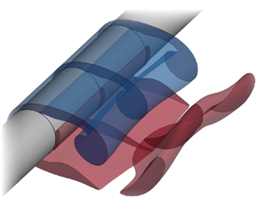
This implies that, to leading order, long-wavelength perturbations to the two-dimensional base flow self-organise so that the flow in each streamwise slice corresponds to the base flow at shifted times, where the amount of shift depends on the spanwise coordinate,  $z$. This is illustrated in the conceptual sketch in figure 5.

Figure 5. Illustration of the time-shifting pattern for the three-dimensionally perturbed flow: the flow in each streamwise slice is given by the two-dimensional flow at a slightly different time; the time shift depends on the spanwise coordinate  $z$. (a) Two-dimensional base flow within streamwise slices at slightly different times. (b) Resulting three-dimensional perturbed flow.
Furthermore, substituting (5.6) into (5.5) shows that the equation for  $w_1$ is uncoupled from the other perturbations,
 \begin{equation} \frac{\mathcal{D} w_1}{\mathcal{D}t} ={-}\dot{P}+\frac{1}{{\textit{Re}}}\nabla^2w_1,\end{equation}
and hence the leading-order spanwise flow is driven exclusively by the pulsations of the base flow pressure,  $\dot {P}(\boldsymbol {r},t)$.
The perturbation to the vorticity is given by
 \begin{equation} \left(\begin{array}{c} \omega_x' \\ \omega_y' \\ \omega_z' \end{array}\right)=\tau \left[\left(\begin{array}{c} 0 \\ 0 \\ \dot{\varOmega} + O(\gamma^2) \end{array}\right)\cos(\gamma z) + \left(\begin{array}{c} \gamma\left(\dot{V}-{\partial w_1}/{\partial y}\right) + O(\gamma^3)\\ \gamma\left({\partial w_1}/{\partial x}-\dot{U}\right) + O(\gamma^3)\\ 0 \end{array}\right) \sin(\gamma z)\right]. \end{equation}
This shows that for small wavenumbers, the perturbations to the vorticity are dominated by the spanwise component,  $\omega '_z$, which is largest in regions where the time derivative of the base flow vorticity, $\dot {\varOmega }$, is large. This is consistent with the observation that, in the course of the mode A instability, the vortex cores in the base flow undergo considerable spanwise wavy deformations (here due to the $\cos (\gamma z)$ term); see, for example, Barkley & Henderson (Reference Barkley and Henderson1996) and Jiang et al. (Reference Jiang, Cheng, Draper, An and Tong2016a).
The comparison of the in-plane perturbation velocity for mode A at  $\gamma =0$ (obtained by time differentiation of the base-flow solution) with cases at $\gamma \neq 0$ in figure 3 shows that the perturbation pattern in the vortex formation region is still qualitatively similar to $(\dot {U}, \dot {V})$ even when $\gamma$ is not small and ${\textit {Re}}>{\textit {Re}}_A$ (at least up to $\gamma =2.2$ and ${\textit {Re}}=220$ according to figure 3). Furthermore, figure 6 shows that the pattern of the perturbations remains unchanged even at lower ${\textit {Re}}$. Although, formally, the leading-order approximation is no longer valid when $\gamma$ is not small (e.g. in figure 2, it is evident that the leading order term does not describe the dependence $\sigma (\gamma )$ for large $\gamma$), the persistence of the time-shifting pattern in the vortex formation region indicates its significant role in the onset of mode A. This suggests that the spatial structure of the mode A instability can be explained by the mechanism for the formation of the time-shifting pattern discussed above.

Figure 6. Pattern of perturbations at  ${\textit {Re}}=100,150$ and $\gamma =0, 0.8$, and $1.6$: perturbation energy $e$ (greyscale colour contours) and in-plane ( $z=0$) perturbation velocity (arrows). Solid lines are the base flow vorticity isolines $\varOmega =\pm 1$. All plots are snapshots at $t=0.5T$, corresponding to the minimum of the lift coefficient. Perturbations at $\gamma =0$ are obtained by time differentiation of the base flow solution, see (5.2). One should not directly compare the magnitude of perturbations in the different cases; it is defined up to a constant factor which we adjusted manually to highlight the similarities and differences of the perturbations patterns.
The symmetry of mode A behind a circular cylinder is inherited from the two-dimensional base flow. Williamson (Reference Williamson1996b) observed it experimentally and gave a physical explanation based on the suggested self-sustaining process. Barkley & Henderson (Reference Barkley and Henderson1996) extracted the symmetry relations by examining numerically obtained eigenfunctions from the linear stability analysis:
 \begin{equation} \begin{pmatrix} u_p\\ v_p\\ w_p\\ p_p \end{pmatrix}(x,y,t+T/2)=\begin{pmatrix} u_p\\ -v_p\\ w_p\\ p_p \end{pmatrix}(x,-y,t). \end{equation}
For a base flow with the symmetry (3.1), only two types of synchronous bifurcations to the three-dimensional flow are allowed (Marques, Lopez & Blackburn Reference Marques, Lopez and Blackburn2004; Blackburn, Marques & Lopez Reference Blackburn, Marques and Lopez2005): preserving (like mode A) and breaking (like mode B) the base-flow symmetry. In this context, the instabilities with the Floquet branch connected to the neutral mode at  $\gamma =0$ belong to the former group: the neutral mode has the base-flow symmetry and, consequently, the time-shifting pattern inherits it as well (e.g. see relation (5.6)). However, it is not evident whether all the modes that exhibit the symmetry (5.12) are caused by a common physical mechanism.
We note that none of the above analysis relies on the geometry of the cylinder, implying that our results are equally applicable to flows past other bluff bodies for which mode A instabilities are observed. In particular, the time-shifting pattern is observed even when the base flow is non-symmetric, e.g. in the flow past an elliptic cylinder at an incidence angle (Rao et al. Reference Rao, Leontini, Thompson and Hourigan2017) and in the flow past a rotating cylinder (Rao et al. Reference Rao, Radi, Leontini, Thompson, Sheridan and Hourigan2015). Therefore, the time-shifting pattern can serve as an additional unifying characteristic of certain mode A type three-dimensional instabilities.
6. Physical mechanisms for flow instability
The previous section showed that in the small-wavenumber limit, small-amplitude three-dimensional perturbations to the two-dimensional time-periodic base flow are dominated by a simple time shifting of that base flow. Comparison against the numerical solution of the perturbation equations showed that this pattern persists up to wavenumbers at which the base flow becomes unstable to the mode A instability. The approach, therefore, successfully predicts the flow pattern at the onset of the three-dimensional instability, but it does not explain why these perturbations grow for a specific range of wavenumbers at fixed Reynolds number (e.g. at  ${\textit {Re}}=220$, it corresponds to $1.1<\gamma <2.1$, as illustrated in figure 2).
To address this issue, we now analyse the various physical mechanisms that affect the growth or decay of such three-dimensional perturbations. For this purpose, we define the in-plane perturbation velocity  $\boldsymbol {v}(\boldsymbol {r}, t)=(v_x,v_y, 0)$ and vorticity $\boldsymbol {\zeta }(\boldsymbol {r}, t)=(\zeta _x,\zeta _y, 0)$ by the relations
 \begin{equation} \left.\begin{gathered}
\boldsymbol{u}'\left(\boldsymbol{x},
t\right)=(v_x,v_y,0)\cos(\gamma z)+\left(0, 0,
v_z\right)\sin(\gamma z),\\
\boldsymbol{\omega}'\left(\boldsymbol{x},
t\right)=(\zeta_x,\zeta_y,0)\sin(\gamma z)+ \left(0,0,
\zeta_z\right)\cos(\gamma z).
\end{gathered}\right\}
\end{equation}
\begin{equation} \left.\begin{gathered}
\boldsymbol{u}'\left(\boldsymbol{x},
t\right)=(v_x,v_y,0)\cos(\gamma z)+\left(0, 0,
v_z\right)\sin(\gamma z),\\
\boldsymbol{\omega}'\left(\boldsymbol{x},
t\right)=(\zeta_x,\zeta_y,0)\sin(\gamma z)+ \left(0,0,
\zeta_z\right)\cos(\gamma z).
\end{gathered}\right\}
\end{equation}
Using the definition of the three-dimensional vorticity,  $\boldsymbol {\omega }'=\boldsymbol {\nabla }\times \boldsymbol {u}'$, and the fact that the three-dimensional perturbation velocity $\boldsymbol {u}'$ is divergence-free shows that these two-dimensional fields are related via
 \begin{equation} \boldsymbol{\zeta}=\gamma (v_{y}, -v_{x},0)+ \frac{1}{\gamma}\left(-\frac{\partial{\boldsymbol{\nabla}\boldsymbol{\cdot}\boldsymbol{v}}}{\partial y}, \frac{\partial{\boldsymbol{\nabla}\boldsymbol{\cdot}\boldsymbol{v}}}{\partial x},0\right). \end{equation}
The rate of change of the two-dimensional perturbation vorticity  $\boldsymbol {\zeta }$ is governed by the linearised vorticity transport equation
 \begin{equation} \frac{\mathcal{D} \boldsymbol{\zeta}}{\mathcal{D}t}= \underbrace{\boldsymbol{\mathsf{E}} \boldsymbol{\cdot} \boldsymbol{\zeta}}_{stretching} \underbrace{+\frac{1}{2}\boldsymbol{\varOmega}\times\boldsymbol{\zeta}}_{rigid\ rotation} \underbrace{+\frac{1}{{\textit{Re}}}\left(\underbrace{\nabla^{2} \boldsymbol{\zeta}}_{\textit{in-plane}}- \underbrace{\gamma^{2} \boldsymbol{\zeta}}_{spanwise}\right)}_{viscous\ diffusion} \underbrace{-\gamma \varOmega \boldsymbol{v}}_{tilting}, \end{equation}
where  $\boldsymbol {\varOmega } = (0,0,\varOmega )$. Each term on the right-hand side of (6.3) has a clear physical interpretation and explains the material rate of change of the perturbation vorticity $\boldsymbol {\zeta }$ in terms of vortex stretching by the base flow rate-of-strain field $\boldsymbol{\mathsf{E}}$; the re-orientation of the vorticity vector by the rigid body rotation of fluid particles in the base flow; the in-plane and spanwise viscous diffusion of the perturbation vorticity; and the tilting of the base flow vortex due to spanwise shear. See Appendix B for more details.
To facilitate the subsequent analysis, we combine (6.2) and (6.3) by exploiting that the perturbation vorticity,  $\boldsymbol {\omega }'$, is divergence-free and that for an incompressible fluid, $\nabla ^2\boldsymbol {u}'=-\boldsymbol {\nabla }\times \boldsymbol {\omega }'$. This implies that
 \begin{equation} \nabla^2\boldsymbol{v}-\gamma^2\boldsymbol{v}=\gamma\boldsymbol{\zeta}_{\bot}+\frac{1}{\gamma}\boldsymbol{\zeta}_{\Delta}, \end{equation}
where
 \begin{equation} \boldsymbol{\zeta}_{\bot}(\boldsymbol{r}, t)=\left(\zeta_{y},-\zeta_{x},0 \right),\quad \boldsymbol{\zeta}_{\Delta}(\boldsymbol{r}, t) =\left(-\boldsymbol{\nabla}\boldsymbol{\cdot}\frac{\partial\boldsymbol{\zeta}}{\partial y}, \boldsymbol{\nabla}\boldsymbol{\cdot}\frac{\partial\boldsymbol{\zeta}}{\partial x},0\right). \end{equation}
The screened Poisson equation (6.4) determines the in-plane velocity perturbation  $\boldsymbol {v}$ in terms of the in-plane perturbation to the vorticity, $\boldsymbol {\zeta }$. An explicit relation between the two fields can therefore be obtained by introducing the Green's function $G_\gamma (\boldsymbol {r}, \boldsymbol {r}')$, which satisfies
 \begin{equation} \left.\begin{gathered}
\nabla^2G_\gamma-\gamma^2G_\gamma=\delta(\boldsymbol{r}-\boldsymbol{r}'),\\
G_\gamma=0\quad \text{at } r=0.5,\\
G_\gamma\rightarrow0\quad \text{as } r\rightarrow\infty.
\end{gathered}\right\} \end{equation}
\begin{equation} \left.\begin{gathered}
\nabla^2G_\gamma-\gamma^2G_\gamma=\delta(\boldsymbol{r}-\boldsymbol{r}'),\\
G_\gamma=0\quad \text{at } r=0.5,\\
G_\gamma\rightarrow0\quad \text{as } r\rightarrow\infty.
\end{gathered}\right\} \end{equation}
We show in Appendix C that the solution to (6.6) is given by
 \begin{equation} G_\gamma(\boldsymbol{r}, \boldsymbol{r}')={-}\frac{1}{2{\rm \pi}}K_0(\gamma|\boldsymbol{r}- \boldsymbol{r}'|)+\frac{1}{2{\rm \pi}}\sum_{m={-}\infty}^{\infty} \frac{I_m(\gamma/2)K_m(\gamma r)K_m(\gamma r')}{K_m(\gamma/2)}\cos m(\varphi-\varphi'), \end{equation}
where  $I_m(r)$ and $K_m(r)$ are the modified Bessel functions of the first and second kind; $\boldsymbol {r}=r(\cos \varphi, \sin \varphi )$ and $\boldsymbol {r}'=r'(\cos \varphi ', \sin \varphi ')$.
Using this expression, the in-plane perturbation velocity  $\boldsymbol {v}$ is given by
 \begin{equation} \boldsymbol{v}(\boldsymbol{r},t)=\int_{D}\gamma G_\gamma(\boldsymbol{r},\boldsymbol{r}') \boldsymbol{\zeta}_{\bot}\left(\boldsymbol{r}',t\right)+\frac{1}{\gamma}G_\gamma(\boldsymbol{r},\boldsymbol{r}') \boldsymbol{\zeta}_{\Delta}\left(\boldsymbol{r}',t\right){\rm d} \boldsymbol{r}', \end{equation}
where  $D$ is the exterior of the cylinder. Substituting this into (6.3) yields
 \begin{align} \frac{\mathcal{D} \boldsymbol{\zeta}}{\mathcal{D}t} &= \underbrace{\boldsymbol{\mathsf{E}} \boldsymbol{\cdot} \boldsymbol{\zeta}}_{stretching} +\underbrace{\frac{1}{2}\boldsymbol{\varOmega}\times\boldsymbol{\zeta}}_{rigid\ rotation} +\underbrace{\frac{1}{{\textit{Re}}}\left(\underbrace{\nabla^{2} \boldsymbol{\zeta}}_{{in\text{-}plane}}- \underbrace{\gamma^{2} \boldsymbol{\zeta}}_{spanwise}\right)}_{viscous\ diffusion} \nonumber\\ &\quad \underbrace{-\,\varOmega \int_{D}\gamma^2 G_\gamma(\boldsymbol{r}, \boldsymbol{r}') \boldsymbol{\zeta}_{\bot}\left(\boldsymbol{r}',t\right)+G_\gamma(\boldsymbol{r}, \boldsymbol{r}')\boldsymbol{\zeta}_{\Delta}\left(\boldsymbol{r}',t\right){\rm d} \boldsymbol{r}'}_{tilting}, \end{align}
which describes the evolution of perturbations to the flow entirely in terms of the perturbations to the in-plane vorticity,  $\boldsymbol {\zeta }$. The equation shows that the first three physical mechanisms are local in the sense that their contribution to the rate of change of $\boldsymbol {\zeta }$ depends only on $\boldsymbol {\zeta }$ or its spatial derivatives. Conversely, tilting is a global effect – the rate of change of $\boldsymbol {\zeta }$ due to the final term depends on $\boldsymbol {\zeta }$ and its derivatives throughout the domain. Furthermore, (6.9) shows how variations in the two parameters ${\textit {Re}}$ and $\gamma$ affect the various mechanisms. The wavenumber only affects the spanwise diffusion and the tilting mechanism. The effect of variations in the Reynolds number is more subtle: it has a direct effect on the strength of the viscous diffusion but also affects the base flow and, thus, the stretching, rigid rotation and tilting mechanisms (via $\boldsymbol{\mathsf{E}}$ and $\varOmega$). We will now analyse the importance of these mechanisms in detail.
6.1. Effect of the viscous diffusion and the base flow
The Reynolds number simultaneously affects the base flow and the intensity of the in-plane and spanwise viscous diffusion. To study the contribution of these three effects separately, we replace the Reynolds number in front of the diffusion terms in (6.9) by  ${\textit {Re}}'$ and ${\textit {Re}}''$, and thus write the evolution equation for the in-plane perturbation to the vorticity, $\boldsymbol {\zeta }$, as
 \begin{align} \frac{\mathcal{D} \boldsymbol{\zeta}}{\mathcal{D}t}&= \underbrace{\boldsymbol{\mathsf{E}} \boldsymbol{\cdot} \boldsymbol{\zeta}}_{stretching} +\underbrace{\frac{1}{2}\boldsymbol{\varOmega}\times\boldsymbol{\zeta}}_{rigid\ rotation} +\underbrace{\underbrace{\frac{1}{{\textit{Re}}'}\nabla^{2} \boldsymbol{\zeta}}_{{in\text{-}plane}}- \underbrace{\frac{\gamma^{2}}{{\textit{Re}}''} \boldsymbol{\zeta}}_{spanwise}}_{viscous\ diffusion} \nonumber\\ &\quad \underbrace{-\,\varOmega \int_{D}\gamma^2 G_\gamma(\boldsymbol{r}, \boldsymbol{r}')\boldsymbol{\zeta}_{\bot}\left(\boldsymbol{r}',t\right)+ G_\gamma(\boldsymbol{r}, \boldsymbol{r}')\boldsymbol{\zeta}_{\Delta}\left(\boldsymbol{r}',t\right){\rm d} \boldsymbol{r}'}_{tilting}. \end{align}
Here the  ${\textit {Re}}$-dependent base flow affects the base-flow rate-of-strain tensor, $\boldsymbol{\mathsf{E}}$, and the base-flow vorticity, $\varOmega$.
Figure 7 illustrates the contributions that the mechanisms discussed so far make to the destabilisation of the flow as the Reynolds number is increased from 180 to 200. The two solid lines show the Floquet multipliers  $\mu$ for the actual flow (i.e. when ${\textit {Re}}={\textit {Re}}'={\textit {Re}}''$) at Reynolds numbers ${\textit {Re}}=180$ and $200$. The remaining broken lines show the destabilising effects of the modification only in the base flow (blue line, ${\textit {Re}}=200,{\textit {Re}}'={\textit {Re}}''=180$), in-plane viscous diffusion (red line, ${\textit {Re}}'=200,{\textit {Re}}={\textit {Re}}''=180$) and spanwise viscous diffusion (green line, ${\textit {Re}}''=200,{\textit {Re}}={\textit {Re}}'=180$). (We obtained the curves corresponding to distinct ${\textit {Re}}$ and ${\textit {Re}}'$ by modifying the input data, feeding our stability code with the pre-computed base flow at ${\textit {Re}}$, while using ${\textit {Re}}'$ in the stability equations; the impact of the spanwise viscous diffusion ( ${\textit {Re}}''$) was assessed explicitly, see below.) For the wavelengths over which the mode A instability arises, the modification to the base flow and the in-plane viscous diffusion can be seen to have a considerable (and comparable) effect on the destabilisation of the flow, whereas the spanwise viscous diffusion only plays a minor role in this process.

Figure 7. Influence of the Reynolds number on the dominant Floquet multiplier near the onset of instability ( ${\textit {Re}}_A\approx 190$). Two solid black lines correspond to the actual Floquet multiplier $\mu$ ( ${\textit {Re}}={\textit {Re}}'={\textit {Re}}''$), other lines represent the Floquet multiplier obtained as a result of independent variation of the base flow ( ${\textit {Re}}$; blue), in-plane ( ${\textit {Re}}'$; red) and spanwise ( ${\textit {Re}}''$; green) viscous diffusion.
The overall effect of the spanwise viscous diffusion can be taken into account explicitly using the change of variables
 \begin{equation} \boldsymbol{\tilde{\zeta}}(\boldsymbol{r}, t) = \boldsymbol{\zeta}(\boldsymbol{r}, t) \exp(\gamma^2t/{\textit{Re}}), \end{equation}
which transforms (6.9) into an identical equation for  $\boldsymbol {\tilde {\zeta }}$, but with the spanwise diffusion term removed. Equation (6.11), therefore, implies that in the absence of spanwise viscous diffusion, the Floquet multiplier $\mu$ would change to
 \begin{equation} \tilde{\mu} = \mu \exp(\gamma^2 T/Re) >\mu, \end{equation}
meaning that spanwise viscous diffusion is always stabilising, and that it does not have an effect on the spatial pattern of the perturbations. An increase in Reynolds number or a decrease in wavenumber both reduce the stabilising effect of the spanwise viscous diffusion. (We note that the period of the vortex shedding,  $T$, also depends on the Reynolds number; however, for the regime considered here, $T$ decreases with ${\textit {Re}}$ and, therefore, does not affect our statement.)
6.2. Effect of the tilting mechanism
Figure 2 shows that the dependence of the dominant Floquet multiplier,  $\mu$, on the wavenumber $\gamma$ is non-monotonic: $\mu (\gamma =0)=1$, corresponding to the neutral stability of the base flow to the time-shifting pattern discussed in § 5. The dominant Floquet multiplier then decreases with increasing $\gamma$ before it rises again, ultimately leading to the onset of the mode A instability for $1.1<\gamma <2.1$ at ${\textit {Re}}=220$.
Only the tilting and spanwise diffusion depend on the wavenumber and, as discussed above, the latter effect is always stabilising; more so, in fact, as  $\gamma$ is increased. The destabilisation of the base flow at sufficiently large $\gamma$ must, therefore, be due to the tilting of the base flow vorticity due to spanwise shear ( $\boldsymbol {v}\cos (\gamma z)$). Equation (6.8) shows that this mechanism is a non-local effect: $\boldsymbol {v}$ is induced by the perturbation to the in-plane vorticity, $\boldsymbol {\zeta }$, everywhere in the flow, in a manner similar to Biot–Savart induction.
The strength of this non-local interaction is defined by two kernel functions  $G_\gamma (\boldsymbol {r}, \boldsymbol {r}')$ and $\gamma ^2 G_\gamma (\boldsymbol {r}, \boldsymbol {r}')$ in (6.9). They are determined by the problem geometry and describe how much the perturbations at point $\boldsymbol {r}$ are affected by the in-plane vorticity and its second derivatives at point $\boldsymbol {r}'$. Both kernel functions are singular at $\boldsymbol {r} = \boldsymbol {r}'$ and decay with an increase in $|\boldsymbol {r} - \boldsymbol {r}'|$. We illustrate the spatial variation of $G_\gamma (\boldsymbol {r}, \boldsymbol {r}')$ in figure 8(b) for the case where $\boldsymbol {r}$ (identified by the red star symbol) is located at the instantaneous local maximum of the perturbation vorticity in the flow shown in figure 8(a). An increase in $\gamma$ makes both kernel functions more localised, as illustrated by the orange isolines, along which $G_\gamma (\boldsymbol {r}, \boldsymbol {r}') = -10^{-1.6}$. We note that an increase in $\gamma$ causes $G_\gamma (\boldsymbol {r}, \boldsymbol {r}')$ to decrease throughout the domain; conversely, the magnitude of $\gamma ^2 G_\gamma (\boldsymbol {r}, \boldsymbol {r}')$ increases in the vicinity of $\boldsymbol {r}$, enhancing the influence that the vorticity in the proximity of a given point has on the growth of the perturbations at that point.

Figure 8. The contribution of perturbation distribution to their growth or decay at the local maximum of  $\zeta$ (marked with the star symbol) through the tilting mechanism at ${\textit {Re}}=220$, various $\gamma$ and $t=0.44T$. (a) In-plane perturbation vorticity: $\log _{10}\zeta$. (b) Kernel function $\log _{10} |G_\gamma (\boldsymbol {r},\boldsymbol {r}')|$. (c) Contribution to the tilting mechanism at point $\boldsymbol {r}$ (the star symbol): $\mathcal {T}(\boldsymbol {r},\boldsymbol {r}',t)$. The orange lines highlight the isoline of kernel function $G_\gamma (\boldsymbol {r}, \boldsymbol {r}')$, shown in panel (b). Solid lines in panels (a,c) are isolines $\kappa =1$ (the boundaries of the elliptic regions). Perturbation vorticity is normalised so that the local maximum of $\zeta$ (star symbol) equals 1.
To determine the effect of the tilting mechanism on the actual growth rate of perturbations in a given flow, we multiply (6.9) by  $\boldsymbol {\zeta }$ to obtain
 \begin{equation} \frac{1}{2}\frac{\mathcal{D} \zeta^2}{\mathcal{D}t}= \underbrace{\boldsymbol{\zeta}\boldsymbol{\cdot}\boldsymbol{\mathsf{E}} \boldsymbol{\cdot} \boldsymbol{\zeta}}_{stretching} \underbrace{+\frac{1}{{\textit{Re}}}\left(\boldsymbol{\zeta}\boldsymbol{\cdot}\nabla^{2} \boldsymbol{\zeta}-\gamma^{2} \zeta^2\right)}_{viscous\ diffusion} \underbrace{+ \int_{D}\mathcal{T}(\boldsymbol{r},\boldsymbol{r}', t)\,{\rm d} \boldsymbol{r}'}_{tilting}, \end{equation}
where  $\zeta = |\boldsymbol {\zeta }|$ and
 \begin{equation} \mathcal{T}(\boldsymbol{r},\boldsymbol{r}',t) ={-}G_\gamma(\boldsymbol{r}, \boldsymbol{r}') \varOmega(\boldsymbol{r}, t)\boldsymbol{\zeta}(\boldsymbol{r}, t)\boldsymbol{\cdot}\left[\gamma^2 \boldsymbol{\zeta}_{\bot}\left(\boldsymbol{r}',t\right)+\boldsymbol{\zeta}_{\Delta}\left(\boldsymbol{r}',t\right)\right]. \end{equation}
When  $\mathcal {T}(\boldsymbol {r},\boldsymbol {r}',t)$ is positive/negative, the perturbations in the vicinity of point $\boldsymbol {r}'$ tend to increase/decrease the magnitude of perturbations $\zeta$ at point $\boldsymbol {r}$.
Let us consider examples of the distribution of  $\mathcal {T}$ at various $\gamma$ and fixed ${\textit {Re}}=220$ at time $t=0.44T$, which corresponds to the early stage of perturbation development in the forming vortex (cf. the illustration of the entire cycle in figure 9a). The greyscale contours in figure 8(a) illustrate the magnitude of the perturbation to the in-plane vorticity (on a logarithmic scale), normalised so that its local maximum at the location indicated by the star (the local maximum of $\zeta$ in the forming vortex) is equal to 1 in all cases. An increase in $\gamma$ leads to a strong increase in the magnitude of $\zeta$ as the perturbation develops; compare, e.g. the magnitude of $\zeta$ in the braid region for $\gamma =0.4$ and $\gamma =2.2$. This increase of $\zeta$ (and the derived quantities, $\boldsymbol {\zeta }_{\bot }$ and $\boldsymbol {\zeta }_{\Delta }$) is counteracted by the increasing localisation of the kernel functions, as illustrated by the isolines $G_\gamma (\boldsymbol {r}, \boldsymbol {r}') = -10^{-1.6}$ from figure 8(b). (The contribution of $\gamma ^2 G_\gamma (\boldsymbol {r}, \boldsymbol {r}') \boldsymbol {\zeta }_{\bot }$ to the tilting integral in (6.13) turns out to be negligible, so the isoline of $G_\gamma (\boldsymbol {r}, \boldsymbol {r}')$ gives a good indication of the domain of influence for the tilting mechanism.)

Figure 9. Local growth of perturbations at  ${\textit {Re}}=220$ and $\gamma =1.6$: (a) in-plane perturbation vorticity $\log _{10}\zeta$; (b) local maximum $\zeta _{max}(t)$ (red line), which corresponds to the star symbol in panel (a). In panel (b), we also show similar curves for stable cases at ${\textit {Re}}=220$ (dashed black lines) and ${\textit {Re}}=50$ (dotted blue line). Solid lines in panel (a) are isolines $\kappa =1$ (the boundaries of the elliptic regions). Perturbation vorticity is normalised so that at $t=0.44T$, the local maximum of $\zeta$ (star symbol) equals one.
The red/blue colours (representing positive/negative values of  $\mathcal {T}$) in figure 8(c) highlight which regions in the flow destabilise/stabilise the flow at point $\boldsymbol {r}$ and thus identify the significant non-local interactions of perturbations in various flow subregions. A key feature in figure 8(c) is that previously formed perturbations outside the forming vortex (particularly in the hyperbolic region) have a noticeable effect on the development of newly created perturbations in the vortex core. This raises questions about the validity of simplified models that attempt to explain the instability based on isolated flow features.
Figure 8(c) shows that, as expected, when  $\gamma$ increases, the non-local interactions become more localised: the contribution to the growth of $\zeta$ at point $\boldsymbol {r}$ weakens more rapidly with the distance, even though surrounding perturbations become more intense at higher $\gamma$ (cf. figure 8a). Incidentally, another confirmation of more localised interactions of perturbations can be found in figures 3 and 6, where, with an increase in $\gamma$, the induced in-plane perturbation velocity, $\boldsymbol {v}$, can be seen to become smaller far from the regions where the perturbations in $\zeta$ concentrate; cf. (6.8).
Thus, the range of wavenumbers,  $\gamma$, for which three-dimensional perturbations are unstable is determined by the tilting mechanism (recall that the uniformly stabilising action of the spanwise diffusion is explicitly taken into account by (6.12)). The tilting mechanism operates via non-local interactions between perturbations in different parts of the domain. The strength of these interactions is controlled by the spanwise wavenumber $\gamma$ through the kernel functions $G_\gamma$ and $\gamma ^2 G_\gamma$, which become more localised with an increase in $\gamma$.
6.3. Local growth and feedback
We will now use these results to analyse the subtle balance between the local growth of perturbations and their feedback on the newly developing perturbations that are generated during the next period of the time-periodic base flow. As discussed in § 1, our analysis can be confined to the vortex formation region, recognised as the origin of three-dimensional instability (Barkley Reference Barkley2005; Giannetti et al. Reference Giannetti, Camarri and Luchini2010).
For this purpose, figure 9(a) shows the time evolution of the three-dimensional perturbations, characterised by logarithmic contours of the perturbation to the in-plane vorticity,  $\zeta$, over one period of the time-periodic base flow for ${\textit {Re}}=220$ and $\gamma =1.6$. We note that for these values, the flow is unstable with a Floquet multiplier of $\mu = 1.25$. The symbols in figure 9(a) indicate the location $\boldsymbol {r}_M(t)$ of the local maximum of $\zeta$, which we follow from its inception in the forming vortex (figure 9ai) as it is swept through the domain (figure 9aii–viii). We normalised the perturbation so that at $t=0.44T$, the maximum is equal to 1, and show the subsequent evolution of $\zeta _{max}(t) = \zeta (\boldsymbol {r}_M(t),t)$ using the red line in figure 9(b).
The maximum is initially located in the elliptic region where the flow is dominated by rotation (figure 9ai–iv). This is the region in which the elliptic instability is commonly assumed to operate, and the perturbations can be seen to grow rapidly. At  $t \approx 0.97T$, $\boldsymbol {r}_M(t)$ crosses the boundary of the elliptic region (identified by the white solid lines in figure 9a) and enters the hyperbolic region, where the flow is dominated by strain. Interestingly, $\zeta _{max}(t)$ can be seen to undergo a second phase of strong growth when it enters this region, and over one period of the time-periodic base flow (starting at $t=0.44T$), $\zeta _{max}(t)$ increases by a factor of $6$.
$6$.
In this particular case, the tilting-induced feedback to the region where the next maximum is formed is strong enough to result in an overall flow instability with a Floquet multiplier of  $\mu = 1.25$. Hence, at $t=1.44T$, when the cycle is about to repeat itself, the amplitude of the next maximum of the perturbation in the vortex formation region is $\mu = 1.25$ times bigger than during the previous cycle. This process then repeats itself with every new cycle (at least until nonlinearities, which are not included in our analysis, become significant).
The other lines in figure 9(b) illustrate the temporal evolution of the maximum perturbation for other values of the parameters  $\gamma$ and ${\textit {Re}}$. An increase in $\gamma$ generally leads to stronger local growth, but this does not necessarily strengthen the overall instability. For instance, when $\gamma = 2.2$, $\zeta _{max}(t)$ increases by a factor of 8 over one period. Yet, despite this more rapid local growth, the overall flow is actually restabilised ( $\mu = 0.92$). This can be explained by the weakening of the feedback using the analysis presented in § 6.2. Indeed, the variation of $\gamma$ primarily affects the flow (and the amount of feedback in particular) through the tilting mechanism, i.e. through non-local interactions of perturbations. Figure 8 illustrates that these interactions become more localised as $\gamma$ increases. Consequently, although the perturbations become more intense, they are not sufficiently felt during the formation of the next local maximum, resulting in a weakened feedback.
Similarly, it is interesting to note that even when the Reynolds number is reduced to  ${\textit {Re}} = 50 < {\textit {Re}}_A\approx 190$, a regime where the flow is strongly stable, with $\mu = 0.28$, $\zeta _{max}(t)$ still undergoes a noticeable local growth. However, it remains too weak to provide sufficient positive feedback to the formation of perturbations during the next cycle.
7. Conclusions
We studied the onset of three-dimensional mode A instability in the near wake behind a circular cylinder. Our analysis showed that long-wavelength perturbations organise in a time-shifting pattern so that the in-plane part  $(u, v, p)(x,y,z,t)$ of the perturbed velocity field is connected to the two-dimensional base flow $(U, V, P)(x,y,t)$ by the relation
 \begin{equation} (u, v, p)(x,y,z,t)\approx(U, V, P)\left(x,y,t+\tau\cos(\gamma z)\right), \end{equation}
where  $\tau (t)$ describes the exponential growth of the instability, here assumed to remain small enough to justify the use of linearised equations for the perturbations. The spanwise component of the velocity perturbation is driven by fluctuations in the base flow pressure, $\dot {P}$.
While these predictions are based on the assumption of a small wavenumber,  $\gamma \ll 1$, comparisons against the results from a numerical Floquet analysis showed that they provide a good qualitative description of the three-dimensional flow over a range of wavenumbers and Reynolds numbers, including the regime where the flow changes from being stable to being unstable to three-dimensional perturbations.
We therefore analysed the mechanisms which control the growth or decay of three-dimensional perturbations and established their dependence on the two non-dimensional parameters (the Reynolds number  ${\textit {Re}}$ and the wavenumber $\gamma$). It turned out that near the onset of the instability ( ${\textit {Re}}\sim {\textit {Re}}_A$), changes in the base flow and the intensity of in-plane viscous diffusion with ${\textit {Re}}$ are essential in flow destabilisation (having comparable contributions); in contrast, the relative effect of spanwise viscous diffusion is negligible. The analysis also highlighted the crucial role played by the tilting mechanism, which operates via non-local interactions, similar to Biot–Savart induction. We characterised its domain of influence using a Green's function-based approach, which allowed us to rationalise the non-trivial dependence of the growth rate on the wavenumber $\gamma$: for $\gamma =0$, the base flow is neutrally stable, corresponding to a Floquet multiplier of $\mu =1$; for small positive values of $\gamma$, the growth rate of three-dimensional perturbations becomes negative, $\mu < 1$; it then reaches a minimum before increasing, finally reaching the onset of the mode A instability when $\mu > 1$. We attributed this behaviour to two competing effects: an increase in $\gamma$ leads to a more rapid local growth of the perturbations as they are swept along by the flow. However, the action of the tilting mechanism becomes more localised, weakening the feedback from existing perturbations on the perturbations that are being generated during the next period of the time-periodic base flow.
While our analysis was performed for flows past circular cylinders, none of the technical details rely on the specific geometry and, therefore, can be useful in studying other instabilities that transform into the time-shifting mode as the spanwise wavenumber tends to zero. For example, additional simulations (not shown here) indicate that the long-wavelength modes  $\hat {\textrm {A}}$ and G behind an elliptic and rotating cylinder exhibit the same time-shifting pattern. This is consistent with the Floquet analyses of Rao et al. (Reference Rao, Leontini, Thompson and Hourigan2013) and Leontini et al. (Reference Leontini, Lo Jacono and Thompson2015).
Acknowledgements
The authors would like to acknowledge the assistance given by Research IT, and the use of the HPC Pool funded by the Research Lifecycle Programme at the University of Manchester.
Funding
The research was supported by a Newton International Fellowship funded by the Royal Society (NIF $\backslash$R1 $\backslash$201343).
Declaration of interests
The authors report no conflict of interest.
Appendix A. Numerical method
We solve the problems for the base flow (§ 3) and perturbations (§ 4) numerically in a bounded domain  $D$, which is restricted by the surface of the cylinder ( $x^2+y^2=0.25$) and an artificial far boundary. The position of the latter is chosen so that the resulting distortion of the flow in the region of interest is negligible (see § A.3): the input, output and side boundaries are located at $x=-30$, $x=50$ and $y=\pm 30$, respectively. The boundary conditions are shown in figure 10.

Figure 10. Schematic representation of the problem (dimensionless formulation) with artificial far boundary and corresponding boundary conditions shown in blue.
A.1. Discretisation of the problem
We apply the second-order stabilised finite element method for the spatial discretisation of the corresponding problems on a triangulated domain  $D$ (see figure 11). Stabilisation techniques used in the present work are PSPG (pressure-stabilising/Petrov–Galerkin) and SUPG (streamline-upwind/Petrov–Galerkin) (Brooks & Hughes Reference Brooks and Hughes1982; Tezduyar Reference Tezduyar1991; Tezduyar et al. Reference Tezduyar, Mittal, Ray and Shih1992). They introduce stabilisation terms (in the weak formulation of the problem) constituting a residual-based technique to overcome two restrictions of the standard Galerkin method. The first one is that the LBB (Ladyzhenskaya–Babuška–Brezzi) condition (Brezzi & Fortin Reference Brezzi and Fortin1991) does not allow to use the same polynomial degree for pressure and velocity interpolation; and the second one is the instability caused by the nonlinear terms for convection-dominated flows. Stabilisation terms used in the present work are similar to those used by Mittal & Kumar (Reference Mittal and Kumar2003) and Kumar & Mittal (Reference Kumar and Mittal2006) to solve the linearised Navier–Stokes equations for two-dimensional stability analyses. We employ a second-order scheme for the temporal discretisation, which involves extrapolating the nonlinear advection and stabilisation terms to obtain a linear system of algebraic equations when seeking the base-flow solution. When solving the linearised Navier–Stokes equations for perturbations, the stabilisation terms are linearly dependent on the unknowns.

Figure 11. Triangulation of computational domain  $D$ (mesh $M_0$): (a) the entire domain and (b) the region near the cylinder.
The resulting system of linear equations for the base flow consists of  $3N$ real-valued equations, and for the perturbations, it has $4N$ complex equations, where $N$ is the number of mesh nodes. At each time step, these systems are solved by the biconjugate gradient stabilised method (BiCGSTAB) with an algebraic multigrid (AMG) preconditioner, implemented with the use of the Portable, Extensible Toolkit for Scientific Computation (PETSc) (Balay et al. Reference Balay2022a,Reference Balayb). The parallel calculations are MPI-based, with the distribution of the work among computational nodes based on a mesh partition performed with ParMETIS (Karypis Reference Karypis2011). The calculations were carried out on the HPC Pool and Computational Shared Facility at the University of Manchester.
A.2. Finding eigensolutions
The Floquet multipliers coincide with the eigenvalues of the monodromy operator  $\boldsymbol{\mathsf{P}}^{\textrm {T}}$, which maps the perturbations at $t=t_0$ to the one at $t=t_0+T$. The action of this operator was found by solving the linearised Navier–Stokes equations for perturbations. For this purpose, we computed the two-dimensional base flow in advance and stored 80 time instants within the vortex shedding period. As done by Barkley & Henderson (Reference Barkley and Henderson1996), we then used the Fourier representation of the base flow to evaluate it at any instant. Eigenvalues and eigenfunctions of $\boldsymbol{\mathsf{P}}^{\textrm {T}}$ were found using Arnoldi iterations, producing orthonormal vectors $\boldsymbol {q}_1,\boldsymbol {q}_2,\ldots, \boldsymbol {q}_m$ that span the Krylov subspace and tridiagonal $m\times m$ Hessenberg matrix. The eigenvalues $\lambda$ and eigenfunctions $\boldsymbol {q}$ of this matrix give an approximation for the dominant eigensolutions of $\boldsymbol{\mathsf{P}}^{\textrm {T}}$. In our calculations, we set the dimension of the Krylov subspace $m$ to values between $15$ and $25$.
$25$.
To validate our results (see figure 2), we used an alternative approach to finding the Floquet multipliers – by directly solving linearised Navier–Stokes equations with random initial conditions (equivalent to the power method) and tracking how the solution changes after several periods of vortex shedding. For more details on both approaches, see Barkley & Henderson (Reference Barkley and Henderson1996), Tuckerman & Barkley (Reference Tuckerman and Barkley2000), and Blackburn & Lopez (Reference Blackburn and Lopez2003).
A.3. Testing
All the results presented in the main part of the paper are obtained using time step  ${\rm \Delta} t=0.002$ and mesh $M_0$ shown in Figure 11 and described in detail in table 1. Figure 12 shows the comparison of the mean drag coefficient $\overline {C_D}$ and the Strouhal number $St$ (defined by the oscillation frequency of lift coefficient $C_L(t)$) with the curves obtained by fitting into the two-dimensional numerical simulations (Henderson Reference Henderson1995; Williamson & Brown Reference Williamson and Brown1998) and experimental data (Fey, König & Eckelmann Reference Fey, König and Eckelmann1998). In the range $30\le {\textit {Re}}\le 300$, $\overline {C_D}$ and $St$ differ from these data by less than $1.7\,\%$.

Figure 12. Comparison of mean pressure  $\overline {C_{D_p}}$, friction $\overline {C_{D_f}}$ and total $\overline {C_D}$ drag coefficients and Strouhal number $St$ with the fitting curves by Henderson (Reference Henderson1995), Williamson & Brown (Reference Williamson and Brown1998), and Fey et al. (Reference Fey, König and Eckelmann1998) for the two-dimensional base flow at $30\le {\textit {Re}}\le 300$.
Table 1. Computational domains and meshes used in the paper.

Table 2 shows the sensitivity of the mean drag coefficient  $\overline {C_D}$, amplitude of lift coefficient ${\rm \Delta} C_L$ and Strouhal number $St$ at ${\textit {Re}}=300$ to:
(i) time resolution – ${\rm \Delta} t=2\times 10^{-3}$ and $10^{-3}$;
(ii) space resolution – twice larger and smaller step compared to mesh
$M_0$ (see table 1);(iii) sizes of the computational domain – twice larger distances to the cylinder from the inlet, outlet and side boundaries (see table 1).


Values of  $\overline {C_D}$, ${\rm \Delta} C_L$ and $St$ given in table 2 are obtained using the data over 83 cycles of oscillations on the interval $200< t<600$. The variations in $\overline {C_D}$, ${\rm \Delta} C_L$ and $St$ are less than $0.7\,\%$. Figure 13(a,b) shows the influence of spatial and temporal resolution on the distribution of vorticity.

Figure 13. (a,b) Sensitivity of vorticity distribution at  ${\textit {Re}}=300$ to the parameters of the numerical method. (c,d) Flow periodicity in the entire domain at ${\textit {Re}}=220$ and $300$. Solid lines are isolines $\varOmega =\pm 0.3$. The snapshots correspond to the maximum of the lift coefficient reached as $t$ exceeds 600. (a) Various spatial resolution ( ${\rm \Delta} t=10^{-3}$): $M_0$, $M_{2h}$, and $M_{0.5h}$ – black, blue and red lines. (b) Various temporal resolution ( $M_0$): ${\rm \Delta} t=2\times 10^{-3}$ and $10^{-3}$ – black and red lines. (c) Periodicity check at ${\textit {Re}}=220$: times $t$ and $t+T$ – black and red lines. (d) Periodicity check at ${\textit {Re}}=300$: times $t$ and $t+T$ – black and red lines.
Table 2. Sensitivity of the base flow simulations at  ${\textit {Re}}=300$ to the parameters of the numerical method and comparison with the data of Henderson (Reference Henderson1995), Williamson & Brown (Reference Williamson and Brown1998) and Fey et al. (Reference Fey, König and Eckelmann1998) (using the expressions for the fitting curves). The last three columns show the relative difference compared to the reference data in the first row (corresponds to the parameters chosen for our simulations in the main part of the text): $(c-c_{ref})/c_{ref}$.

At the transition to the secondary vortex street, one might also expect the emergence of the additional frequency in the wake (Cimbala, Nagib & Roshko Reference Cimbala, Nagib and Roshko1988), which could raise a question of the applicability of the Floquet analysis. However, in our case, it is absent due to the choice of the domain size (Jiang & Cheng Reference Jiang and Cheng2019) – figures 13(c) and 13(d) show visual periodicity checks at  ${\textit {Re}}=220$ and $300$.
The Floquet multiplier agrees with the data of Barkley & Henderson (Reference Barkley and Henderson1996) (extracted by digitising their figure 7), see figure 2. In addition, the figure shows that two approaches to finding eigensolutions (the Arnoldi iterations and the power method, see § A.2) give consistent results.
Appendix B. Growth and decay of perturbation vorticity in fluid particles
This section describes the basic physical mechanisms affecting the growth or decay of perturbation vorticity in fluid particles (Aleksyuk & Shkadov Reference Aleksyuk and Shkadov2018, Reference Aleksyuk and Shkadov2019). The following alternative form of (6.3) can be derived using the polar representation of in-plane velocity  $\boldsymbol {v}=v(\cos \theta _1, \sin \theta _1)$ and vorticity $\boldsymbol {\zeta }=\zeta (\cos \theta, \sin \theta )$ vectors,
 \begin{equation} \left.\begin{gathered} \frac{\mathcal{D} \ln \zeta}{\mathcal{D}t}=S \cos 2 \alpha-\frac{\gamma \varOmega v}{\zeta} \cos \beta+\frac{1}{{\textit{Re}}}\left(\frac{\boldsymbol{\zeta} \boldsymbol{\cdot} \nabla^{2} \boldsymbol{\zeta}}{\zeta^{2}}-\gamma^{2}\right),\\ \frac{\mathcal{D} \theta}{\mathcal{D}t}={-}S \sin 2 \alpha-\frac{\gamma \varOmega v}{\zeta} \sin \beta+\frac{1}{{\textit{Re}}} \frac{\boldsymbol{\zeta} \times \nabla^{2} \boldsymbol{\zeta}}{\zeta^{2}} \boldsymbol{\cdot} \boldsymbol{e}_{3}+\frac{1}{2}\varOmega, \end{gathered}\right\} \end{equation}
where  $\alpha (x, y, t)=\theta -\varPhi ; \beta (x, y, t)=\theta _{1}-\theta$; and $\boldsymbol {e}_3$ is the unit vector in the spanwise direction. This form reveals two key quantities of the base flow defining the evolution of perturbations: the dominant stretching rate ( $S$) and rotation rate ( $\varOmega /2$).
According to (6.3), the rate of  $\boldsymbol {\zeta }$ change in a fluid particle (of the base flow) is defined by the action of the following four basic physical mechanisms.
(i) First term in (6.3): perturbation vortex stretching by the base flow strain field. Let us illustrate its action by omitting other terms on the right-hand side of (B1) and assuming that
$S$ and $\varPhi$ are constant in a fluid particle (without the loss of generality, $\varPhi =0$). The solution of these equations with initial condition $\boldsymbol {\zeta }=(\zeta _x^0, \zeta _y^0)$ is $\zeta _x=\zeta ^0_x \exp ({St})$, $\zeta _y=\zeta ^0_y \exp ({-St})$. The in-plane perturbation vorticity vector in a fluid particle exponentially tends to align with the stretching direction, $\tan \alpha = \exp ({-2St})$, while its endpoint continues to belong to hyperbole $\zeta _x\zeta _y=\zeta ^0_x \zeta ^0_y$. The sketch for the action of this mechanism is shown in figure 14(a).(ii) Second term in (6.3): rotation of a fluid particle as a rigid body. This mechanism does not change the amplitude of
$\boldsymbol {\zeta }$; it only rotates this vector with angular velocity $\varOmega /2$. Figure 14(b,c) shows examples of the combined action of this mechanism with stretching in the case of constant $S$, $\varOmega$ and $\varPhi =0$ in a fluid particle. In this case, the solution of (B1) can be written in the form of a conic section: $\zeta _x^2-2\kappa \zeta _x\zeta _y+\zeta _y^2+C=0$, where $C$ is a constant defined by initial conditions.
Figure 14. Action of (a–c) stretching and (d) tilting on in-plane perturbation vorticity vector
$\boldsymbol {\zeta }$. Panels (a), (b) and (c) correspond to the cases $\varOmega=0$, $ 0 < \varOmega/2 < S$ and $S<\varOmega/2$, respectively. The shaded regions in panels (a–c) show where $\boldsymbol {\zeta }$ grows; in panel (d), it shows where tilting (vector $-\gamma \varOmega \boldsymbol {v}{\rm \Delta} t$) causes growth of $\boldsymbol {\zeta }$. The shades of the red vector show the evolution of $\boldsymbol {\zeta }$.If
$\kappa >1$, the solution (hyperbole) has the following dependence on time:
(B2)where\begin{equation} \boldsymbol{\zeta}(t)=A(1, \kappa-\chi) \exp({\varOmega \chi t/2})+B(\kappa-\chi, 1)\exp({-\varOmega \chi t/2}), \end{equation}$\chi =\sqrt {|\kappa ^2-1|}$, and constants $A$ and $B$ are defined by the initial conditions. With the increase in time, vector $\boldsymbol {\zeta }$ tends to the asymptote $\zeta _y=(\kappa -\chi )\zeta _x$. The schematic representation of this solution is given in figure 14(b).
If
$\kappa <1$, the solution (ellipse) is
(B3)where the initial conditions define constants\begin{equation} \boldsymbol{\zeta}(t)=A(1, \kappa)\cos\left[\varOmega\chi (t-t_0)/2\right]+A(0, \chi) \sin\left[\varOmega\chi (t-t_0)/2\right], \end{equation}$A$ and $t_0$. The major axis of the ellipse is $\zeta _y=\zeta _x$. The schematic representation of this solution is given in figure 14(c). When rotation prevails, the stretching mechanism itself (without tilting) cannot provide the overall growth of perturbations. For example, in the case of elliptic instability, the role of the tilting is to create parametric resonance by aligning the perturbation with the base flow strain field so that the perturbation has overall growth due to stretching. More details are given by Kerswell (Reference Kerswell2002).(iii) Third term in (6.3): viscous diffusion of vorticity. In (6.3), this mechanism is decoupled into two parts: in-plane (
${\textit {Re}}^{-1}\partial ^2/\partial x^2+{\textit {Re}}^{-1}\partial ^2/\partial y^2$) and spanwise ($-\gamma ^2/{\textit {Re}}$) diffusion. Using the change of variables $(\boldsymbol {v}, \boldsymbol {\zeta })=(\boldsymbol {\tilde {v}}, \boldsymbol {\tilde {\zeta }})\exp (-\gamma ^2t/{\textit {Re}})$, we eliminate term $\gamma ^2\boldsymbol {\zeta }/{\textit {Re}}$. This gives a clear idea on the exponential viscous stabilisation. In-plane viscous diffusion depends on a local perturbation pattern but commonly has a stabilising effect.(iv) Fourth term in (6.3): base flow vortex tilting due to spanwise shear. Without viscous forces, vortex lines are ‘frozen’ into fluid, and, on a short time interval
${\rm \Delta} t$, the spanwise shear $\boldsymbol {v}\cos \gamma z$ at $\gamma z={\rm \pi} /2$ adds $-\gamma \varOmega \boldsymbol {v}{\rm \Delta} t$ to perturbation vorticity $\boldsymbol {\zeta }$ (see figure 14d).


Appendix C. Green's function for the screened Poisson equation on the disk exterior
The solution of (6.6) in the unbounded domain is  $-K_0(\gamma |\boldsymbol {r}- \boldsymbol {r}'|)/(2{\rm \pi} )$, where $K_0(r)$ is the modified Bessel function of the second kind. In the bounded domain, the homogeneous boundary conditions for the Green's function can be satisfied by introducing function $g_\gamma (\boldsymbol {r}, \boldsymbol {r}')$:
 \begin{equation} G_\gamma(\boldsymbol{r}, \boldsymbol{r}') ={-}\frac{1}{2{\rm \pi}}\left[K_0(\gamma |\boldsymbol{r}- \boldsymbol{r}'|)+g_\gamma(\boldsymbol{r}, \boldsymbol{r}')\right], \end{equation}
defined as a solution of the system
 \begin{equation} \left.\begin{gathered}
\nabla^2 g_\gamma-\gamma^2g_\gamma =0,\\
g_\gamma={-}K_0(\gamma |\boldsymbol{r}-
\boldsymbol{r}'|),\quad \text{at } r=0.5,\\
g_\gamma\rightarrow0,\quad \text{as } r\rightarrow\infty.
\end{gathered}\right\} \end{equation}
\begin{equation} \left.\begin{gathered}
\nabla^2 g_\gamma-\gamma^2g_\gamma =0,\\
g_\gamma={-}K_0(\gamma |\boldsymbol{r}-
\boldsymbol{r}'|),\quad \text{at } r=0.5,\\
g_\gamma\rightarrow0,\quad \text{as } r\rightarrow\infty.
\end{gathered}\right\} \end{equation}
Seeking the solution in the form
 \begin{equation} g_\gamma(\boldsymbol{r}, \boldsymbol{r}')=\sum_{m={-}\infty}^{\infty}g^m_\gamma(r, r')\cos m(\varphi-\varphi') \end{equation}
and using (8) of Watson (Reference Watson1952, § 11.3) at  $r=0.5$ and $r'>r$:
 \begin{equation} K_0(\gamma |\boldsymbol{r}- \boldsymbol{r}'|)=\sum_{m={-}\infty}^{\infty}I_m(\gamma/2)K_m(\gamma r')\cos m(\varphi-\varphi'), \end{equation}
we obtain the following problems for  $g^m_\gamma (r, r')$:
 \begin{equation} \left.\begin{gathered} \displaystyle \frac{\partial^2 g^m_\gamma}{\partial r^2}+\frac{1}{r} \frac{\partial g^m_\gamma}{\partial r}-\left(\frac{m^2}{r^2}+\gamma^2\right)g^m_\gamma =0,\\ \displaystyle g^m_\gamma={-}I_m(\gamma/2)K_m(\gamma r')\quad \text{at } r=0.5,\\ \displaystyle g^m_\gamma\rightarrow0\quad \text{as } r\rightarrow\infty. \end{gathered}\right\} \end{equation}
The solution of this system is the modified Bessel function of the second kind:
 \begin{equation} g^m_\gamma(r, r')={-}\frac{I_m(\gamma/2)K_m(\gamma r')}{K_m(\gamma/2)}K_m(\gamma r). \end{equation}
Thus, by combining (C1), (C3) and (C6), we obtain the expression (6.7).


 Open access