


1. Introduction
Wake interactions between individual horizontal axis wind turbines can reduce wind farm energy production by 10–20 % (Barthelmie et al. Reference Barthelmie, Hansen, Frandsen, Rathmann, Schepers, Schlez, Phillips, Rados, Zervos and Politis2009). Utility-scale wind turbines are controlled to maximize individual power production, rather than collective wind farm production (Boersma et al. Reference Boersma, Doekemeijer, Gebraad, Fleming, Annoni, Scholbrock, Frederik and van Wingerden2017). Individual operation entails aligning each wind turbine in the farm with the incoming wind direction. In contrast, wake steering, where individual wind turbines are intentionally yaw-misaligned with respect to the incident wind direction, has emerged as a promising strategy to reduce wake interactions and increase collective wind farm power production (e.g. Gebraad et al. Reference Gebraad, Teeuwisse, Van Wingerden, Fleming, Ruben, Marden and Pao2016; Bastankhah & Porté-Agel Reference Bastankhah and Porté-Agel2019; Kheirabadi & Nagamune Reference Kheirabadi and Nagamune2019; Zong & Porté-Agel Reference Zong and Porté-Agel2021; Howland et al. Reference Howland, Ghate, Quesada, Pena Martínez, Zhong, Larrañaga, Lele and Dabiri2022a). Maximizing collective wind farm power production through wake steering control generally involves a trade-off between the power lost by the yaw-misaligned turbines and the power gained by the downwind-waked turbines, compared to standard individual control (e.g. Fleming et al. Reference Fleming, Gebraad, Lee, van Wingerden, Johnson, Churchfield, Michalakes, Spalart and Moriarty2015). Since the power-maximizing yaw misalignment angles for wake steering control are estimated primarily using simplified analytical flow models (Gebraad et al. Reference Gebraad, Teeuwisse, Van Wingerden, Fleming, Ruben, Marden and Pao2016; Fleming et al. Reference Fleming, King, Dykes, Simley, Roadman, Scholbrock, Murphy, Lundquist, Moriarty and Fleming2019; Howland et al. Reference Howland, Quesada, Martinez, Larrañaga, Yadav, Chawla, Sivaram and Dabiri2022), it is important to accurately model the dependence of wind turbine power production and wake velocities on the yaw misalignment angle.
Wind turbine power production generally decreases as a function of an increasing yaw misalignment ( $\gamma$) magnitude since the component of the wind velocity that is perpendicular to the rotor decreases. Textbooks instruct that the power production of a yawed wind turbine will decrease following $\cos ^3(\gamma )$ (Burton et al. Reference Burton, Jenkins, Sharpe and Bossanyi2011). This estimate is based on the application of classical one-dimensional momentum theory with an incoming axial freestream wind speed $u_\infty \cos (\gamma )$ perpendicular to the rotor. However, wind turbines extract power from the winds at the rotor. The wind at the rotor is affected by the velocity induced by the wind turbine. Since the induction depends on the wind turbine thrust force, and the thrust force will decrease in yaw misalignment, the induction will depend on the yaw misalignment. The $\cos ^3(\gamma )$ model neglects the dependence of the induction on the yaw misalignment (Micallef & Sant Reference Micallef and Sant2016). Given the error incurred by the $\cos ^3(\gamma )$ model, most analytical wind farm power models assume that the power of a yaw-misaligned wind turbine follows $P_r(\gamma ) = P(\gamma )/P(\gamma =0)=\cos ^{P_p}(\gamma )$, where $P_p$ is an empirical, turbine-specific factor that needs to be tuned using experimental data (Dahlberg & Montgomerie Reference Dahlberg and Montgomerie2005; Gebraad et al. Reference Gebraad, Teeuwisse, Van Wingerden, Fleming, Ruben, Marden and Pao2016). However, such experiments are costly, since they require sustained operation of utility-scale wind turbines in suboptimal yaw misalignment angles (Howland et al. Reference Howland, González, Martínez, Quesada, Larranaga, Yadav, Chawla and Dabiri2020c). Further, the wide spread in $P_p$ values reported in the literature, typically $1< P_p< 3$, suggests that the cosine model is not universal to different turbine models (Dahlberg & Montgomerie Reference Dahlberg and Montgomerie2005; Schreiber et al. Reference Schreiber, Nanos, Campagnolo and Bottasso2017; Liew, Urbán & Andersen Reference Liew, Urbán and Andersen2020; Howland et al. Reference Howland, González, Martínez, Quesada, Larranaga, Yadav, Chawla and Dabiri2020c). Accurate analytical predictions of $P_r(\gamma )$ remain an outstanding challenge (Hur et al. Reference Hur, Berdowski, Simao Ferreira, Boorsma and Schepers2019) – as a starting point, in this study, we focus on analytical predictions of the induction and power production of yawed actuator disks.
Through analysis of an autogyro aircraft, Glauert (Reference Glauert1926) developed an equation for the area-averaged induction and the coefficient of power as a function of the yaw misalignment  $\gamma$. Glauert (Reference Glauert1926) also identified that the induction of a yawed actuator disk varies over the rotor area about its mean value – this finding has been replicated in other actuator disk simulations and models (see review by Hur et al. Reference Hur, Berdowski, Simao Ferreira, Boorsma and Schepers2019). Glauert's yawed actuator disk momentum theory is commonly used in blade-element momentum (BEM) models of rotational wind turbine aerodynamics (see e.g. review by Micallef & Sant Reference Micallef and Sant2016). Using the Bernoulli equation, Shapiro, Gayme & Meneveau (Reference Shapiro, Gayme and Meneveau2018) proposed an equation for the dependence of the axial induction factor on the yaw misalignment of an actuator disk. Speakman et al. (Reference Speakman, Abkar, Martínez-Tossas and Bastankhah2021) used the axial induction equation proposed by Shapiro et al. (Reference Shapiro, Gayme and Meneveau2018) to model $P_r(\gamma )$ for a simulation with thrust coefficient $0.75$, which yielded improved power predictions compared to the $\cos ^3(\gamma )$ model, but higher predictive error than a tuned $\cos ^{P_p}(\gamma )$ with $P_p$ set to $1.88$.
Beyond modelling the power–yaw relationship (i.e.  $P_r(\gamma )$), modelling the inviscid near-rotor wake region of a yawed actuator disk is important since inviscid models are often used as an initial condition for turbulent wake models that are used to predict wind farm power production (Frandsen et al. Reference Frandsen, Barthelmie, Pryor, Rathmann, Larsen, Højstrup and Thøgersen2006; Bastankhah & Porté-Agel Reference Bastankhah and Porté-Agel2016; Shapiro et al. Reference Shapiro, Gayme and Meneveau2018). Therefore, it is equally important to accurately model the induction and the streamwise and spanwise velocity deficits at the outlet of the inviscid near-wake region for a yawed actuator disk.
Finally, a line of research parallel to wake steering has investigated methods for axial induction flow control, where individual wind turbines reduce the magnitude of their wind speed wake deficits by decreasing the thrust force (Annoni et al. Reference Annoni, Gebraad, Scholbrock, Fleming and van Wingerden2016). A promising flow control methodology combines wake steering and induction control (Munters & Meyers Reference Munters and Meyers2018) – for such combined control, it is important to model the joint effect of the yaw misalignment and the wind turbine thrust coefficient on the power and wake deficit.
In this study, classical, inviscid momentum theory is extended to the yaw-misaligned actuator disk. Analytical expressions are developed for the rotor-normal induction, the streamwise velocity deficit, the spanwise velocity deficit, the thrust, and the power production of an actuator disk as a function of yaw misalignment. In § 2, a model is proposed based on a combination of momentum conservation, mass conservation and the Bernoulli equation. The model is validated against large eddy simulations (LES) of a yawed actuator disk. The numerical set-up of the LES is given in § 3, and results are provided in § 4. The model is validated against the LES in § 4.1. The dependence of the induction, velocity deficits and the power on the wind turbine thrust coefficient is presented in § 4.2. Further, in § 4.2 the model is optimized to find the thrust coefficient that maximizes power for each value of the yaw misalignment angle. In § 4.3, the induction model is used as an initial condition for a turbulent far-wake model. The implications of the developed induction–yaw model on quasi-steady wake steering and induction control are presented and discussed. Conclusions are provided in § 5.
2. Yawed actuator disk momentum theory
Our goal is to model the induction, thrust, wake deficit and deflection, and the power production of a yaw-misaligned actuator disk. For the following analysis, we assume that the flow is inviscid and frictionless. We assume that the velocity is continuous across the actuator disk, including both the streamwise and spanwise velocities, and that the pressure recovers to the incident freestream pressure away from the actuator disk. We note that the pressure recovery assumption is relevant to only the Bernoulli equation and streamwise momentum analysis. We do not apply this pressure recovery assumption to a lateral momentum balance, since it is well-known to introduce predictive error (Shapiro et al. Reference Shapiro, Gayme and Meneveau2018) due to counter-rotating vortices in the wake of yawed turbines (Howland et al. Reference Howland, Bossuyt, Martínez-Tossas, Meyers and Meneveau2016). We consider uniform inflow (in  $y$ and
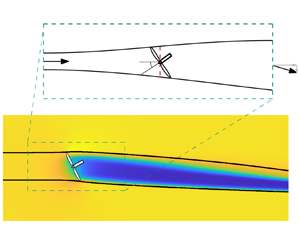
  $z$), as in standard momentum theory, and an actuator disk model (ADM) representation of the wind turbine forcing (Calaf, Meneveau & Meyers Reference Calaf, Meneveau and Meyers2010; Burton et al. Reference Burton, Jenkins, Sharpe and Bossanyi2011). The ADM is introduced in § 2.1. The lateral velocity is modelled following lifting line theory (Shapiro et al. Reference Shapiro, Gayme and Meneveau2018) (§ 2.2). The induction is modelled by combining the Bernoulli equation, conservation of mass and momentum conservation to a control volume containing the yaw-misaligned actuator disk (§ 2.3). A schematic of the yaw-misaligned actuator disk and the control volume is shown in figure 1.

Figure 1. Control volume for the yawed actuator disk analysis. The streamwise and spanwise directions are  $x$ and $y$, respectively. The actuator-disk-modelled wind turbine is yaw-misaligned at angle $\gamma$, where positive yaw misalignment is a counter-clockwise rotation viewed from above. As in classical momentum theory, we consider four stations for the analysis, and the flow variables are labelled with the corresponding station numbers as subscripts. The cross-sectional areas, streamwise velocities, spanwise velocities, pressures and mass flow rates are denoted $A$,
$A$,  $u$,
$u$,  $v$,
$v$,  $p$ and $\dot {m}$, respectively. The unit vector normal to the yawed actuator disk is shown as $\hat {n}$.
In § 2.3, we develop the equations to predict the induction, thrust, wake deficit and deflection, and the power production of a yaw-misaligned actuator disk. In § 2.4, we consider a limiting case of the developed induction model where the outlet spanwise velocity  $v_4$ is negligible compared to the outlet streamwise velocity $u_4$, i.e. $|v_4| \ll u_4$.
2.1. Actuator disk model
The thrust force from an actuator disk on the surrounding flow depends on the freestream rotor-normal wind speed,  $\boldsymbol {u}_\infty \boldsymbol {\cdot } \hat {n}$:
 \begin{equation} \boldsymbol{F}_{T,{ideal}} =-\tfrac{1}{2} \rho C_T A_d (\boldsymbol{u}_{\infty} \boldsymbol{\cdot} \hat{n})^2 \hat{n}, \end{equation}
where  $\rho$ is the density of the incident air, $C_T$ is the coefficient of thrust, $A_d={\rm \pi} D^2/4$ is the area of the rotor disk, with $D$ the wind turbine rotor diameter, $\hat {n}$ is the unit normal vector perpendicular to the disk, and $\boldsymbol {u}_{\infty }$ is the freestream wind velocity vector (Sørensen Reference Sørensen2011). Wind turbines produce thrust and power based on the wind velocity at the rotor, which has been modified by induction. Thus the empirical thrust coefficient $C_T$ depends on the induction. Additionally, for wind farms in the atmospheric boundary layer, it may be challenging to estimate the value of the freestream reference wind speed $u_\infty$ due to wakes of upstream turbines or heterogeneity in the background flow field. Instead, an ADM is used to model wind turbine forcing, where the thrust force scales with the rotor-normal wind speed at the disk, $\boldsymbol {u}_d \boldsymbol {\cdot } \hat {n}$, rather than the freestream $\boldsymbol {u}_\infty \boldsymbol {\cdot } \hat {n}$ (Calaf et al. Reference Calaf, Meneveau and Meyers2010). The ADM thrust force then depends on a modified thrust coefficient $C_T'$ and the disk velocity (Calaf et al. Reference Calaf, Meneveau and Meyers2010):
 \begin{equation} \boldsymbol{F}_T =-\tfrac{1}{2} \rho C_T^{\prime} A_d (\boldsymbol{u}_{d} \boldsymbol{\cdot} \hat{n})^2 \hat{n}. \end{equation}
Equation (2.2) is used in the ADM implementation in LES used for validation as well as the derivation of the analytical model.
Assuming that the freestream wind is uniform and aligned with the  $x$-direction, the freestream wind vector is $\boldsymbol {u}_\infty = u_\infty \hat {\imath }+ 0 \hat {\jmath }$. In this study, we focus on uniform inflow, where the inflow wind $\boldsymbol {u}_\infty$ does not depend on $y$ or $z$. This follows standard momentum theory (Burton et al. Reference Burton, Jenkins, Sharpe and Bossanyi2011), which avoids additional complexities in modelling turbine performance due to wind shear (Choukulkar et al. Reference Choukulkar, Pichugina, Clack, Calhoun, Banta, Brewer and Hardesty2016; Howland et al. Reference Howland, González, Martínez, Quesada, Larranaga, Yadav, Chawla and Dabiri2020c). However, the disk velocity may include a component in the $y$-direction for yaw-misaligned turbines, and so is generally $\boldsymbol {u}_d = u_{d}\hat {\imath } + v_{d}\hat {\jmath }$. The rotor-normal, rotor-averaged induction factor $a_n$ for a rotor with yaw misalignment angle $\gamma$ is defined as
 \begin{equation} a_n = 1 - \frac{ \boldsymbol{u}_d \boldsymbol{\cdot} \hat{n} }{ u_{\infty} \cos(\gamma)}. \end{equation}
In the yaw-aligned case where  $\hat {n}=\hat {\imath }$, the rotor-normal induction factor $a_n$ reduces to the standard (streamwise) axial induction factor $a = 1 - u_d / u_\infty$. The thrust force written in terms of the rotor-normal induction factor is then
 \begin{equation} \boldsymbol{F}_T =-\tfrac{1}{2} \rho C_T^{\prime} A_d ( 1 - a_n)^2 \cos^2(\gamma)\, u_\infty^2 \left[ \cos{(\gamma)}\,\hat{\imath} + \sin{(\gamma)}\,\hat{\jmath} \right]. \end{equation}
The power for the actuator disk is computed as  $P = -\boldsymbol {F}_T \boldsymbol {\cdot } \boldsymbol {u}_d$.
Rotational utility-scale wind turbines produce a thrust force that depends on the velocity at the turbine (e.g. Burton et al. Reference Burton, Jenkins, Sharpe and Bossanyi2011; Sørensen Reference Sørensen2011; Howland et al. Reference Howland, González, Martínez, Quesada, Larranaga, Yadav, Chawla and Dabiri2020c) – the velocity at the turbine is lower than  $u_\infty$ due to induction. Similarly, the ADM produces a thrust force that is proportional to the disk velocity, which has been modified by induction. The thrust force depends on the yaw misalignment for both utility-scale rotational wind turbines and the ADM. In the ADM, $C_T^{\prime }$ is an input. If we prescribe a value of $C_T^{\prime }$ that does not depend on the yaw angle, then the thrust force of the ADM depends on the yaw misalignment following $F_T(\gamma ) \propto (1-a_n)^2 \cos ^2(\gamma )$. However, since the rotor-normal induction depends on the imposed thrust force $F_T$, and the thrust force decreases with an increasing magnitude of yaw misalignment, we hypothesize that the induction factor will depend on $\gamma$ such that $a_n = a_n(\gamma )$.
The derivation in §§ 2.2 and 2.3 will prescribe an ADM-type forcing where  $C_T^\prime$ is an input quantity. We emphasize that the proposed analytical model can be applied for a wind turbine model for which $C_T^\prime$ varies as a function of the yaw misalignment. This will be demonstrated in § 4.2.
In the model validation against LES in § 4.1, we compare the proposed model to an ADM forcing in LES where  $C_T^\prime$ is a fixed quantity that does not depend on the yaw misalignment (see (2.2)). For different wind turbine models, a different form of the thrust force $F_T$ may be appropriate (i.e. a form different to (2.2)). Specifically, $C_T^\prime$ may not be a fixed quantity, and would be a required, known input to the final model form. In general for rotational turbines, the potential dependence of $C_T^\prime$ on the yaw misalignment will depend on the turbine control strategy (i.e. the blade pitch and torque control) and the wind conditions (Howland et al. Reference Howland, González, Martínez, Quesada, Larranaga, Yadav, Chawla and Dabiri2020c). For a different form of $F_T$, the quantitative model predictions would differ but the qualitative trends of the influence of yaw misalignment on the induction are expected to apply. Further discussion is included in Appendix E using wind tunnel data from Krogstad & Adaramola (Reference Krogstad and Adaramola2012), and the need for future work is highlighted in § 5.
2.2. Lifting line spanwise velocity model with rotor-normal induction depending on yaw
Yaw-misaligned wind turbines generate a counter-rotating vortex pair that deflects and deforms the wake region into a curled wake shape (Bastankhah & Porté-Agel Reference Bastankhah and Porté-Agel2016; Howland et al. Reference Howland, Bossuyt, Martínez-Tossas, Meyers and Meneveau2016; Fleming et al. Reference Fleming, Annoni, Churchfield, Martinez-Tossas, Gruchalla, Lawson and Moriarty2018; Martínez-Tossas et al. Reference Martínez-Tossas, King, Quon, Bay, Mudafort, Hamilton, Howland and Fleming2021). The counter-rotating vortex pair rotates about a low-pressure centre. Momentum balance approaches to predict the lateral velocity in the wake of a yaw-misaligned actuator disk that neglect the influence of the lateral pressure gradient often exhibit predictive errors (Jiménez, Crespo & Migoya Reference Jiménez, Crespo and Migoya2010; Shapiro et al. Reference Shapiro, Gayme and Meneveau2018). Shapiro et al. (Reference Shapiro, Gayme and Meneveau2018) developed a model for the spanwise velocity downwind of a yaw-misaligned actuator disk. The approach uses Prandtl lifting line theory (Milne-Thomson Reference Milne-Thomson1973) to predict the spanwise velocity in the inviscid near-wake region downwind of the actuator disk. The downwash produced by the lifting line theory was presumed to be the spanwise velocity in the outlet of the streamtube enclosing the yawed actuator disk. The resulting model predicts the spanwise velocity disturbance  $\delta v_0 = v_\infty - v_4 = \frac {1}{4} C_T u_\infty \cos ^2(\gamma ) \sin (\gamma )$. The model exhibited excellent predictions of the circulation at the disk hub-height ( $z=0$), defined as $\varGamma _0$ (Shapiro et al. Reference Shapiro, Gayme and Meneveau2018), over a range of yaw and thrust values. The spanwise velocity disturbance $\delta v_0$ was also compared to LES. The predictions exhibited improved accuracy compared to previous models, but had a slight underprediction of $\delta v_0$ at high yaw misalignment angles, $|\gamma |>20^\circ$ (Shapiro et al. Reference Shapiro, Gayme and Meneveau2018).
Following § 2.1, we consider the Prandtl lifting line approach developed by Shapiro et al. (Reference Shapiro, Gayme and Meneveau2018) applied to the ADM with a prescribed  $C_T^\prime$, instead of a prescribed $C_T$. The spanwise velocity disturbance is
 \begin{equation} \delta v_0 = v_\infty - v_4 = \frac{- \varGamma_0}{4R} = \frac{-\boldsymbol{F}_T \boldsymbol{\cdot} \hat{\jmath}}{2 \rho u_\infty A_d} = \frac{1}{4}\,C_T^\prime u_\infty \sin(\gamma) \cos^2(\gamma) \left(1-a_n(\gamma)\right)^2. \end{equation}
Comparing (2.5) to the model proposed by Shapiro et al. (Reference Shapiro, Gayme and Meneveau2018),  $C_T^\prime$ is the input quantity and there is an additional nonlinear dependence on $a_n(\gamma )$. We note that Shapiro et al. (Reference Shapiro, Gayme and Meneveau2018) identified the influence of the yaw misalignment on the induction, and accounted for it by plotting $\delta v_0$ against $C_T$, where the thrust coefficient was estimated empirically as $C_T = C_T^\prime \tilde {u}_{d}^2 / (u_\infty ^2 \cos ^2(\gamma ))$, with $\tilde {u}_d$ the disk velocity measured from the LES validation case. In the following subsections, we will develop a predictive model for $a_n(\gamma )$ that uses (2.5).
2.3. Model for the induction of a yaw-misaligned actuator disk
To model the induction, we first apply the Bernoulli equation from stations 1 to 2 and from stations 3 to 4 within the streamtube, shown in figure 1:
 \begin{equation} \left.\begin{gathered} p_1 + \tfrac{1}{2}\rho \|\boldsymbol{u}_1\|^2 = p_2 + \tfrac{1}{2}\rho \|\boldsymbol{u}_2\|^2, \\ p_3 + \tfrac{1}{2}\rho \|\boldsymbol{u}_3\|^2 = p_4 + \tfrac{1}{2}\rho \|\boldsymbol{u}_4\|^2, \end{gathered}\right\}\end{equation}
where  $\|\boldsymbol {u}_4\| = \sqrt {u_4^2 + v_4^2}$. We note that the outlet flow has non-zero components in the $x$ (
$x$ ( $\hat {\imath }$) and $y$ (
$y$ ( $\hat {\jmath }$) directions, denoted as $u_4$ and $v_4$, respectively (see figure 1). Assuming that the pressure recovers to the freestream at station 4 ( $p_1$ = $p_4 = p_\infty$) and that the velocity across the rotor disk is continuous ( $\boldsymbol {u}_2 = \boldsymbol {u}_3 = \boldsymbol {u}_d$), (2.6) can be combined and simplified to
 \begin{equation} p_2 - p_3 = \tfrac{1}{2}\rho \left( \|\boldsymbol{u}_1\|^2 - \|\boldsymbol{u}_4\|^2 \right). \end{equation}
Substituting in  $\boldsymbol {u}_1 = \boldsymbol {u}_\infty$, $\boldsymbol {u}_4=u_4\hat {\imath } + v_4\hat {\jmath }$ and $(\,p_2 - p_3) A_d = \|\boldsymbol {F}_{T}\|$, with $\boldsymbol {F}_T$ given by (2.4), this becomes
 \begin{equation} u_\infty^2 - u_4^2 - v_4^2 = C_T' (1-a_n)^2 \cos^2(\gamma)\,u_\infty^2. \end{equation}
Next, we apply mass conservation to the streamtube between stations 2 and 4, where  $A_2=A_d$:
 \begin{equation} \boldsymbol{u}_4 \boldsymbol{\cdot} (A_4 \hat{\imath}) = \boldsymbol{u}_2 \boldsymbol{\cdot} (A_2 \hat{n}). \end{equation}
Substituting in  $\boldsymbol {u}_2=\boldsymbol {u}_d$ and the definition of $a_n$ in (2.3), $\boldsymbol {u}_d \boldsymbol {\cdot } \hat {n} = (1-a_n)u_\infty \cos (\gamma )$, this simplifies to
 \begin{equation} u_4 A_4 = (1-a_n) u_\infty \cos(\gamma)\,A_d. \end{equation}
We then apply mass conservation to the two-dimensional control volume, assuming that the flow outside the disk streamtube is unperturbed at  $u_\infty$:
 \begin{align} \dot{m}_{1} + \dot{m}_{2} &=\rho u_{\infty} A_{CV} - \rho u_\infty (A_{CV} - A_4) - \rho u_4 A_4 \nonumber\\ &= \rho A_4 (u_\infty - u_4), \end{align}
where  $CV$ denotes the control volume (figure 1). Finally, we apply conservation of momentum to the control volume in the streamwise direction ( $\hat {\imath }$), using the Reynolds transport theorem assuming steady-state flow:
 \begin{equation} \rho\,\frac{\mathrm{D}u}{\mathrm{D} t} = \int_{CS} \rho u \left(\boldsymbol{u}_{rel} \boldsymbol{\cdot} \mathrm{d}\boldsymbol{A}\right) = \boldsymbol{F}_T \boldsymbol{\cdot} \hat{\imath} + p_1 A_{CV} - p_4 A_{CV}, \end{equation}
where  ${CS}$ is the control surface. By expanding the surface integral and combining terms, this momentum balance simplifies to
 \begin{equation} \boldsymbol{F}_T \boldsymbol{\cdot} \hat{\imath} = \rho u_4^2 A_4 - \rho u_\infty^2 A_4 + (\dot{m}_{1} + \dot{m}_{2}) u_\infty. \end{equation}
Substituting (2.4), (2.10) and (2.11) into (2.13) and simplifying gives
 \begin{equation} -\tfrac{1}{2} C_T^{\prime} u_\infty (1 - a_n) \cos^2(\gamma) = u_4 - u_\infty. \end{equation}
 Finally, we solve for  $a_n$ in (2.8) from Bernoulli, $u_4/u_\infty$ in (2.14) from conservation of mass and the streamwise momentum balance, and $v_4/u_\infty$ in (2.5) from the lifting line spanwise velocity deficit model, resulting in a coupled nonlinear system of three equations to solve for $a_n(\gamma )$, $u_4(\gamma )$ and $v_4(\gamma )$:
 \begin{equation} \left.\begin{aligned} a_n(\gamma) = 1 - \dfrac{\sqrt{u_\infty^2-u_4(\gamma)^2-v_4(\gamma)^2}}{ \sqrt{C_T^\prime}\, u_\infty \cos(\gamma)},\\ \dfrac{u_4(\gamma)}{u_\infty} = 1 - \tfrac{1}{2}\,C_T^\prime \left(1-a_n(\gamma)\right) \cos^2(\gamma),\\ \dfrac{v_4(\gamma)}{u_\infty} =-\tfrac{1}{4}\,C_T^\prime \left(1-a_n(\gamma)\right)^2 \sin(\gamma) \cos^2(\gamma). \end{aligned}\right\} \end{equation}
The system in (2.15) can be solved iteratively from an initial condition from standard, yaw-aligned momentum theory  $a_n^0 = a = \frac {1}{2}(1-\sqrt {1-C_T})=C_T'/(C_T'+4)$ and typically converges in less than five iterations. While the system of equations in (2.15) converges quickly, it does not permit a straightforward solution. In § 2.4, we examine a limiting case of the model where the outlet spanwise velocity is neglected in the Bernoulli equation, $|v_4| \ll u_4$.
With a solution for the normal induction factor  $a_n(\gamma )$ from (2.15), the power for a yaw-misaligned actuator disk is modelled as
 \begin{equation} P(\gamma) =-\boldsymbol{F}_T \boldsymbol{\cdot} \boldsymbol{u}_d = \tfrac{1}{2} \rho C_T^\prime A_d \left(1-a_n(\gamma)\right)^3 u_\infty^3 \cos^3(\gamma). \end{equation}
As discussed in the Introduction, the dependence of wind turbine power production on the yaw misalignment is often described by the power ratio  $P_r(\gamma )$ (e.g. Howland et al. Reference Howland, González, Martínez, Quesada, Larranaga, Yadav, Chawla and Dabiri2020c). The resulting model for the power ratio is
 \begin{equation} P_r(\gamma) = \frac{P(\gamma)}{P(\gamma=0)} = \left[\left(1+\frac{1}{4}\,C_T^\prime\right) (1-a_n(\gamma)) \cos(\gamma) \right]^3, \end{equation}
and the thrust ratio is
 \begin{equation} T_r(\gamma) = \frac{F_T(\gamma)}{F_T(\gamma=0)} = \left[ \left(1+\frac{1}{4}\,C_T^\prime\right) (1-a_n(\gamma)) \cos(\gamma) \right]^2. \end{equation}
 Given the ADM turbine representation, the thrust force scales with the rotor-averaged disk velocity (e.g. Calaf et al. Reference Calaf, Meneveau and Meyers2010). Therefore, the rotor-normal induction factor model in (2.15) is the prediction for the rotor-averaged induction factor, defined in (2.3) as  $a_n$. Due to the yaw misalignment, the induction will also vary as a function of the azimuthal position about its rotor-averaged value (Glauert Reference Glauert1926). Glauert (Reference Glauert1926) modelled this $\hat {a}_n(r,\theta ) = \left \langle a_n(r,\theta )\right \rangle _A + a_n^\prime (r,\theta )$, where $\hat {a}_n(r,\theta )$ is the rotor-normal induction depending on the radial $r$ and azimuthal $\theta$ position, $\left \langle a_n(r,\theta )\right \rangle _A$ is the rotor-averaged induction (referred to as $a_n$ elsewhere in the paper), and $a_n^\prime (r,\theta )$ is the zero-mean, azimuthally dependent deviation from the rotor-averaged induction (Hur et al. Reference Hur, Berdowski, Simao Ferreira, Boorsma and Schepers2019). The azimuthally dependent portion of the induction has been modelled empirically as $a_n^\prime (r,\theta ) = K_x ({r}/{R} )\sin (\theta )$, where $R$ is the rotor radius, and $K_x$ is an empirical factor (Glauert Reference Glauert1926; Hur et al. Reference Hur, Berdowski, Simao Ferreira, Boorsma and Schepers2019). We note that $a_n^\prime (r,\theta )$ averages to zero over the rotor $\left(\left \langle a_n^\prime (r,\theta )\right \rangle _A=0\right)$. Since the ADM thrust ( $F_T$) and power ( $P$) depend on the rotor-averaged velocity, $a_n^\prime (r,\theta )$ will not affect $a_n(\gamma )$, $F_T(\gamma )$ or $P(\gamma )$. For turbine models that apply thrust force unequally across the rotor, such as a blade-element (Howland et al. Reference Howland, González, Martínez, Quesada, Larranaga, Yadav, Chawla and Dabiri2020c) or actuator line (Martínez-Tossas, Churchfield & Leonardi Reference Martínez-Tossas, Churchfield and Leonardi2015) representation, $a_n^\prime (r,\theta )$ can affect $F_T(\gamma )$ and $P(\gamma )$, and therefore must be modelled. We suggest future research on the radial and azimuthal variations of the rotor-normal induction factor for turbines beyond the ADM.
2.4. Limiting case of CV analysis with  $|v_4| \ll u_4$

In this subsection, we consider the limiting case where the outlet spanwise velocity from the streamtube is significantly less than the outlet streamwise velocity,  $|v_4| \ll u_4$. Therefore, the outlet velocity is $\|\boldsymbol {u}_4\| = u_4$. Starting from (2.15), the rotor-normal induction is simplified as
 \begin{equation} a_n(\gamma) = \frac{C_T^\prime \cos^2(\gamma)}{4 + C_T^\prime \cos^2(\gamma)}, \end{equation}
which is also the induction factor reported by Shapiro et al. (Reference Shapiro, Gayme and Meneveau2018), who assumed that the spanwise velocity disturbance appeared infinitesimally downwind of the yawed actuator disk and that it was constant in the streamtube downwind. The streamwise and spanwise velocities are
 \begin{equation} \frac{u_4(\gamma)}{u_\infty} = \frac{4 - C_T^\prime \cos^2(\gamma)}{4 + C_T^\prime \cos^2(\gamma)}, \quad \frac{v_4(\gamma)}{u_\infty} =-\frac{4 C_T^\prime \sin(\gamma) \cos^2(\gamma)}{(4 + C_T^\prime \cos^2(\gamma))^2}. \end{equation}
The streamwise outlet velocity  $u_4(\gamma )$ can also be written in terms of the induction factor $a_n(\gamma )$ such that $u_4(\gamma ) = u_\infty (1 - 2a_n(\gamma ))$, where $a_n(\gamma )$ is given by (2.19). This is analogous to the outlet velocity from one-dimensional momentum $u_4(\gamma =0) = u_\infty (1-2a)$, where $a = a_n(\gamma =0)$ is again the standard axial induction factor.
The power of the yawed actuator disk in this limiting case is
 \begin{equation} P(\gamma) = \frac{32 \rho A_d C_T^\prime \cos^3(\gamma)\,u_\infty^3}{(4+C_T^\prime \cos^2(\gamma))^3}. \end{equation}
The power and thrust ratios in this limiting case are
 \begin{equation} P_r(\gamma) = \left[\frac{(4+C_T^\prime) \cos(\gamma)}{4+C_T^\prime \cos^2(\gamma)}\right]^3, \quad T_r(\gamma) = \left[\frac{(4+C_T^\prime) \cos(\gamma)}{4+C_T^\prime \cos^2(\gamma)}\right]^2. \end{equation}
The power ratio model given by (2.22a) was also reported by Speakman et al. (Reference Speakman, Abkar, Martínez-Tossas and Bastankhah2021), who leveraged the streamwise induction model developed by Shapiro et al. (Reference Shapiro, Gayme and Meneveau2018) (same as (2.19)).
3. Large eddy simulation numerical set-up
Large eddy simulations are performed using an incompressible flow code PadéOps (https://github.com/FPAL-Stanford-University/PadeOps; Ghate & Lele Reference Ghate and Lele2017; Howland, Ghate & Lele Reference Howland, Ghate and Lele2020a). Fourier collocation is used in the horizontal directions and a sixth-order staggered compact finite difference scheme is used in the vertical direction (Nagarajan, Lele & Ferziger Reference Nagarajan, Lele and Ferziger2003). Time advancement uses a fourth-order strong stability preserving variant of the Runge–Kutta scheme (Gottlieb, Ketcheson & Shu Reference Gottlieb, Ketcheson and Shu2011), and the subgrid scale closure uses the sigma subfilter scale model (Nicoud et al. Reference Nicoud, Toda, Cabrit, Bose and Lee2011).
The ADM is implemented with the regularization methodology introduced by Calaf et al. (Reference Calaf, Meneveau and Meyers2010) and further developed by Shapiro, Gayme & Meneveau (Reference Shapiro, Gayme and Meneveau2019a). The ADM forcing depends on the prescribed input of  $C_T^\prime$ (see (2.2)), which is varied independently of the yaw misalignment angle. The discretized turbine thrust force $\boldsymbol {f}(\boldsymbol {x})$ is distributed in the computational domain ( $\boldsymbol {x}$) through an indicator function $\mathcal {R}(\boldsymbol {x})$ as
 \begin{equation} \boldsymbol{f}(\boldsymbol{x}) = \boldsymbol{F}_T\,\mathcal{R}(\boldsymbol{x}). \end{equation}
The thrust force  $\boldsymbol {F}_T$ is computed with (2.2), depending on the disk velocity $\boldsymbol {u}_d$. The indicator function $\mathcal {R}(\boldsymbol {x})$ is constructed from a decomposition $\mathcal {R}(\boldsymbol {x}) = \mathcal {R}_1(x)\,\mathcal {R}_2(y, z)$ given by
 $$\begin{gather} \mathcal{R}_1(x) = \frac{1}{2s} \left[ \mathrm{erf}\left(\frac{\sqrt{6}}{\varDelta} \left(x+\frac s2\right)\right) - \mathrm{erf}\left(\frac{\sqrt{6}}{\varDelta} \left(x-\frac s2\right)\right)\right], \end{gather}$$
 $$\begin{gather}\mathcal{R}_2(y, z) = \frac{4}{{\rm \pi} D^2}\,\frac{6}{{\rm \pi}\varDelta^2} \iint H\left(\frac{D}{2} - \sqrt{y'^2+z'^2}\right) \exp\left(-6\, \frac{(y-y')^2+(z-z')^2}{\varDelta^2}\right)\mathrm{d} y'\,\mathrm{d}z', \end{gather}$$
where  $H(x)$ is the Heaviside function, $\mathrm {erf}(x)$ is the error function, $s$ is the ADM disk thickness, and $\varDelta$ is the ADM filter width. The disk velocity $\boldsymbol {u}_d$, used in the thrust force calculation (2.2), is calculated using the indicator function such that
 \begin{equation} \boldsymbol{u}_d = M\iiint \mathcal{R}(\boldsymbol{x})\,\boldsymbol{u}(\boldsymbol{x}) \,\mathrm{d}^3\boldsymbol{x}, \end{equation}
where  $\boldsymbol {u}(\boldsymbol {x})$ is the filtered velocity in the LES domain, and $M$ is an ADM filter width-dependent correction factor (Shapiro et al. Reference Shapiro, Gayme and Meneveau2019a). Depending on the numerical implementation of the indicator function, particularly the selection of ADM filter width $\varDelta$, the ADM can underestimate the induction and therefore overestimate power production (Munters & Meyers Reference Munters and Meyers2017; Shapiro et al. Reference Shapiro, Gayme and Meneveau2019a). To alleviate this power overestimation for larger ADM filter widths, the disk velocity calculation in (3.4) uses a correction factor $M$ derived by Shapiro et al. (Reference Shapiro, Gayme and Meneveau2019a), which depends on $C_T'$ and the ADM filter width. To compute the correction factor $M$, the Taylor series approximation for the ADM correction factor is used (Shapiro et al. Reference Shapiro, Gayme and Meneveau2019a) such that
 \begin{equation} M = \left( 1 + \frac{C_T'}{4}\,\frac{1}{\sqrt{3{\rm \pi}}}\,\frac{2\varDelta}{D}\right)^{-1}. \end{equation}
 The correction factor given by (3.5) was derived by Shapiro et al. (Reference Shapiro, Gayme and Meneveau2019a) for yaw-aligned actuator disks. For low values of  $\varDelta / D$, the correction factor $M$ has a limited impact on the LES results, and the induction and power follow momentum theory (Shapiro et al. Reference Shapiro, Gayme and Meneveau2019a), but low ADM filter widths can also result in numerical oscillations in the flow field due to the ADM forcing discontinuity. For higher values of $\varDelta / D$ with the correction factor implemented for a yaw-aligned ADM, the thrust force and power predicted by momentum theory are well reproduced, but the induced velocity in the LES domain does not conform to momentum theory due to the wide force smearing fundamental to the larger values of $\varDelta /D$ (see Appendix A, figure 10). In the results presented in § 4 where analysis of the wake flow field is required, to reduce numerical oscillations in the wake, a larger ADM filter width $\varDelta /D = 3h/(2D)$ is used with the correction factor $M$ given by (3.5), where $h = (\varDelta x^2 + \varDelta y^2 + \varDelta z^2)^{1/2}$. In the results presented in § 4 for which only the quantities at the actuator disk are analysed, a smaller ADM filter width of $\varDelta / D = 0.29 h / D = 0.032$ is used such that the correction factor is not required to reproduce the power predicted by momentum theory for the yaw-aligned ADM (see also the discussion by Shapiro et al. Reference Shapiro, Gayme and Meneveau2019a). In all cases, the ADM thickness is $s = 3\varDelta x/2$. More discussion of the ADM numerical set-up and the interactions between the LES results and the ADM filter width and the correction factor is provided in Appendix A.
Consistent with the model derivation (see § 2), simulations are performed with uniform inflow with zero freestream turbulence. Periodic boundary conditions are used in the lateral  $y$-direction. A fringe region (Nordström, Nordin & Henningson Reference Nordström, Nordin and Henningson1999) is used in the $x$-direction to force the inflow to the desired profile with a prescribed yaw angle. All simulations are performed with a domain $L_x=25D$ in length, and cross-sectional size $L_y = 20D$, $L_z=10D$, with $256\times 512\times 256$ grid points. A large cross-section is used to minimize the influence of blockage on the ADM, which changes as a function of turbine yaw. A single turbine is placed inside the domain at the centre of the $y$–
$y$– $z$ plane at a distance $5D$ from the domain inlet in the $x$-direction. Simulations are run for two flow-through times $L_x/u_\infty$ to allow the turbine power output to converge, which is sufficient in these zero freestream turbulence inflow cases (Howland et al. Reference Howland, Bossuyt, Martínez-Tossas, Meyers and Meneveau2016).
4. Results
In this section, the model predictions are compared to results from LES, and the model output is explored to reveal implications for wind farm flow control. In § 4.1, the predictive model developed in § 2 is validated against LES. The dependence of the induction on the coefficient of thrust is demonstrated in the model and in LES (§ 4.1). In § 4.2, the model is optimized to find the thrust coefficients that maximize the coefficient of power as a function of the yaw misalignment angle, and the predictions are compared to LES. Finally, in § 4.3, the model is used as an initial condition for a turbulent far-wake model. The influence of the induction–yaw relationship developed in § 2 on a wake steering test case is explored.
4.1. Comparison between the model and LES
The model for  $P_r(\gamma )$ (2.17) is compared to LES in figure 2 for $C_T^\prime =1.33$ for yaw misalignments $0^\circ \leqslant \gamma \leqslant 50^\circ$. The model developed by Glauert (Reference Glauert1926), with the functional form provided in Appendix B, and the developed model in the limit $|v_4| \ll u_4$ (§ 2.4) are also shown. Finally, $\cos (\gamma )$ and $\cos ^3(\gamma )$ are shown for reference. The model developed in § 2.3 exhibits the lowest predictive error compared to the LES data. Neglecting the lateral velocity in the Bernoulli equation, $|v_4| \ll u_4$ (§ 2.4), results in a consistent overprediction of the power production at all yaw misalignment angles because the portion of momentum redistributed to the spanwise velocity, which does not contribute to power, is neglected. Neglecting the lateral velocity in the Bernoulli equation (2.7) increases the predicted pressure drop, and therefore the thrust force and the power, because the energy in the spanwise velocity is not accounted for in the outlet flow.

Figure 2. (a) Normalized power production for the yawed ADM wind turbine with  $C_T^\prime =1.33$, normalized by the power production for a yaw-aligned ADM wind turbine ( $P(\gamma )/P(\gamma =0)$). The LES results are shown with green dots. The model predictions are given by the ‘Yawed CV’ curve, and the limiting case $|v_4| \ll u_4$ for the model is shown. For reference, $\cos ^3(\gamma )$ and $\cos (\gamma )$ curves are shown in addition to the Glauert model (Appendix B). (b) Zoomed-in version of (a) to highlight the performance of different models. (c) Same as (a) with $\cos (\gamma )$ on the $x$-axis.
The Glauert model results in a larger power overprediction. This overprediction is expected, as discussed in Burton et al. (Reference Burton, Jenkins, Sharpe and Bossanyi2011), since the lift contributions to the thrust in the Glauert model should not contribute to power because it does not contribute to net flow through the disk. The  $\cos (\gamma )$ and $\cos ^3(\gamma )$ curves provide upper and lower bounds, respectively, for the LES data and the model predictions. The commonly assumed $\cos ^3(\gamma )$ model (Burton et al. Reference Burton, Jenkins, Sharpe and Bossanyi2011) underpredicts the power production because the yaw misalignment reduces the thrust force, which in turn reduces the rotor-normal induction and increases the disk velocity and the power production.
The model predictions and LES results for the rotor-normal induction  $a_n(\gamma )$ are shown in figure 3. As with the power production, the most accurate predictions result from the yawed CV model in § 2.3. Assuming negligible lateral velocity (§ 2.4) results in an underprediction of the induction, which therefore results in an overprediction of the disk velocity and the power production (figure 2). The Glauert model overpredicts the induction, but also overpredicts the power, likely because of the lift contributions to thrust, as mentioned previously. We note that this is the Glauert model for the rotor-averaged induction. Therefore, the model for radial and azimuthal induction variations proposed by Glauert (Reference Glauert1926) averages to zero (see § 2). The yawed CV model has increasing predictive error for the induction as a function of the yaw misalignment angle. This increasing error could be due to the assumption that the pressure recovers to freestream pressure downwind (see § 2), which was applied in the Bernoulli equation and in the streamwise momentum balance. The wake of a yaw-misaligned turbine curls due to the formation of a counter-rotating vortex pair (Howland et al. Reference Howland, Bossuyt, Martínez-Tossas, Meyers and Meneveau2016). The counter-rotating vortex pair produces a low-pressure region in the yawed turbine wake that increases in magnitude, relative to the pressure drop at the rotor, with increasing turbine yaw (Shapiro et al. Reference Shapiro, Gayme and Meneveau2018), which is not modelled in the present framework. Future work should consider incorporating a pressure model in this framework.

Figure 3. Normalized rotor-normal, rotor-averaged induction for the yawed ADM wind turbine with  $C_T^\prime =1.33$. The model predictions are given by the ‘Yawed CV’ curve, and the limiting case $|v_4| \ll u_4$ for the model is shown. The Glauert model (Glauert Reference Glauert1926) for the rotor-averaged induction is provided in Appendix B.
The lateral velocity disturbance,  $\delta v_0(\gamma )=v_\infty -v_4=-v_4$, is estimated from LES by averaging the lateral velocity in cross-sections of the actuator disk streamtube (Shapiro et al. Reference Shapiro, Gayme and Meneveau2018). The lateral velocity disturbance $\delta v_0(\gamma )$, estimated as the maximum of the cross-sectional averages over $x$, is shown in figure 4(a) along with model predictions. The maximum value of the lateral velocity disturbance $\delta v_0(\gamma )$ generally occurs approximately $D/2$ downwind of the actuator disk wind turbine. The original $C_T$-based model of Shapiro et al. (Reference Shapiro, Gayme and Meneveau2018) ( $\delta v_0(\gamma ) = \frac {1}{4} C_T u_\infty \cos ^2(\gamma ) \sin (\gamma )$) underpredicts the initial lateral velocity disturbance at higher yaw angles. The model developed here yields improved predictions compared to the original model by including the effect of the yaw misalignment on the induction, which the original expression based on $C_T$ does not include. Since the induction decreases with increasing magnitude of the yaw angle, the disk velocity will increase. The increase in disk velocity increases the actuator disk thrust force, partially counteracting the reduction in thrust force from yaw misalignment. The lateral velocity disturbance based on $C_T^\prime$ and $a_n(\gamma )$ will therefore be larger than a prediction from a model that assumes a fixed $C_T$ as a function of yaw $\gamma$.

Figure 4. (a) Normalized lateral velocity deficit with  $C_T^\prime =1.33$. The model predictions for the lateral velocity depending on $C_T$ are shown by $\delta v_0(C_T)$, where $C_T=0.75$. The model predictions for the lateral velocity depending on the induction model given by (2.15) and $C_T^\prime$ are shown by $\delta v_0(C_T^\prime, a_n)$. (b) Normalized streamwise velocity deficit for the yawed ADM wind turbine with $C_T^\prime =1.33$. The model predictions are given by the ‘Yawed CV’ curve, and the limiting case $|v_4| \ll u_4$ for the model is shown.
Finally, the streamwise velocity disturbance is shown in figure 4(b). The LES streamwise velocity disturbance is estimated similarly to  $\delta v_0$, although the maximum value of $\delta u_0$ generally occurs approximately $2D$ downwind of the actuator disk. The streamwise velocity disturbance associated with the yaw-aligned wind turbine, $\delta u_0/u_\infty =2a(\gamma =0)$, is shown as a reference. The streamwise velocity disturbance depends strongly on the yaw misalignment, therefore assuming $\delta u_0(\gamma \neq 0)/u_\infty =\delta u_0(\gamma =0)/u_\infty =2a(\gamma =0)$ would yield significant predictive errors in a wake model. The full model (§ 2.3) has slightly improved predictions compared to the limit of negligible lateral velocity (§ 2.4), but both model estimates overpredict the streamwise velocity disturbance at larger yaw angles.
The model developed in § 2 reveals that the induction  $a_n$, the power $P$ and the power ratio $P_r$ all depend on both the yaw misalignment and the thrust coefficient $C_T^\prime$. The ADM is simulated in LES over a range of yaw misalignment and $C_T^\prime$ values, where each pair $(\gamma, C_T')$ represents a unique LES case. The influence of $C_T^\prime$ on the power ratio $P_r$ for the LES data and the model (2.17) is shown in figure 5(a). The coefficient of power $C_P$ is shown in figure 5(b). The model predictions exhibit low error, compared to the LES data, over a wide range of yaw and thrust values. We observe that the power reduction by yaw misalignment depends inherently on the value of $C_T^\prime$ (figure 5a), due to the influence of the thrust coefficient $C_T^\prime$ and yaw misalignment on the induction factor $a_n$ (figure 5c). This result suggests that the power lost due to yaw misalignment in a practical field setting will be turbine-specific, since existing turbine designs operate at a wide range of thrust coefficients (see e.g. Hansen Reference Hansen2015). Further, since the thrust coefficient depends on the operating condition and turbine controller (e.g. Ainslie Reference Ainslie1988), the power lost due to yaw misalignment will also vary in time for a given turbine design. Therefore, while an empirically tuned cosine model ( $\cos ^{P_p}(\gamma )$) may yield a sufficiently small error for a single turbine model and operating condition (e.g. region II operation; Pao & Johnson Reference Pao and Johnson2009), it cannot be expected to extrapolate to other wind turbine designs or control regimes. Instead, the physics-based model developed in § 2 can provide a prediction of $P_r(\gamma )$, provided that the thrust force characteristics (i.e. $\boldsymbol {F}_T$ or $C_T^\prime$) are known for the turbine model of interest as a function of yaw misalignment. Future work may integrate the induction–yaw model developed in § 2 into BEM codes (e.g. FAST; Jonkman & Buhl Reference Jonkman and Buhl2005).

Figure 5. (a) Power production for the yawed ADM wind turbine, normalized by the power production for a yaw-aligned ADM wind turbine for various values of  $C_T^\prime$. (b) Coefficient of power $C_P(\gamma )$. (c) Rotor-normal, rotor-averaged induction factor $a_n(\gamma )$.
4.2. Optimizing model power and wake deflection in yaw misalignment with $C_T^\prime$

The induction and power models developed in § 2 and the results in § 4.1 indicate that the power production of a yaw-misaligned actuator disk depends on both the yaw misalignment and the local thrust coefficient  $C_T^\prime$. In yaw alignment, the well-known Betz limit result estimates that the axial induction factor that maximizes the coefficient of power $C_P = 2 P / (\rho A_d u_\infty ^3)$ is $a=1/3$ (e.g. Burton et al. Reference Burton, Jenkins, Sharpe and Bossanyi2011), with a corresponding value of $C_T^\prime = 2$. Here, we estimate the value of $C_T^\prime$ that maximizes $C_P$ as a function of yaw misalignment value. The power produced by the actuator disk is given by (2.16). The maximum power occurs at $C_T^{\prime *}$ such that $\partial P / \partial C_T^{\prime } = 0$. Taking the derivative of (2.16) with respect to $C_T^\prime$ yields
 \begin{equation} \frac{\partial P}{\partial C_T^\prime} = \frac{1}{2}\,\rho A_d (1-a_n)^3 \cos^3(\gamma)\, u_\infty^3 - \frac{3}{2}\,\rho C_T^\prime A_d (1-a_n)^2 \cos^3(\gamma)\,u_\infty^3\, \frac{\partial a_n}{\partial C_T^\prime}. \end{equation}
For the full model ((2.15), § 2.3),  $\partial a_n / \partial C_T^\prime$ does not permit a straightforward analytical solution. To result in an analytical solution, we assume the limit $|v_4| \ll u_4$ (see § 2.4), giving
 \begin{equation} \frac{\partial P}{\partial C_T^\prime} = \frac{128 \rho A_d \cos^3(\gamma)\, u_\infty^3}{(4+C_T^\prime \cos^2(\gamma))^4} \left[1 - \frac{1}{2}\,C_T^\prime \cos^2(\gamma)\right], \end{equation}
and power is maximized ( $\partial P / \partial C_T^{\prime } = 0$) at
 \begin{equation} C_T^{\prime*}(\gamma) = \frac{2}{\cos^2(\gamma)}. \end{equation}
For yaw alignment ( $\gamma =0$), the standard Betz limit result is recovered with $C_T^{\prime *}(\gamma =0)=2$. For yaw misalignment ( $\gamma \neq 0$), the power-maximizing thrust $C_T^{\prime *}(\gamma )$ increases monotonically as a function of increasing yaw misalignment magnitude. To maximize the power production of a yaw-misaligned wind turbine, the turbine should operate at a thrust coefficient different to the standard, optimal Betz value ( $C_T=8/9$, $a=1/3$, $C_T^\prime = 2$). The maximum power production as a function of the yaw misalignment is
 \begin{equation} P^*(\gamma) = \tfrac{8}{27} \rho A_d u_\infty^3 \cos(\gamma), \end{equation}
and the maximum  $C_P$ as a function of the yaw misalignment is
 \begin{equation} C_P^*(\gamma) = \tfrac{16}{27} \cos(\gamma), \end{equation}
which is equivalent to the Betz limit with an additional factor  $\cos (\gamma )$. Therefore, subject to the assumptions discussed in § 2, the minimum power production lost by a yaw-misaligned wind turbine is equal to $\cos (\gamma )$. As such, $\cos (\gamma )$ represents an upper bound for $P_r(\gamma )$ (figure 2) if $C_T^\prime$ is permitted to change.
The model predictions (2.15) for the coefficient of power  $C_P$ depending on the yaw misalignment and the thrust coefficient $C_T^\prime$ are shown in figure 6(a). Additionally, the optimal thrust coefficient $C_T^{\prime *}(\gamma )$, assuming $|v_4| \ll u_4$, is shown. The LES coefficient of power $C_P$, for the simulations with the disk velocity $\boldsymbol {u}_d$ correction $M$ developed by Shapiro et al. (Reference Shapiro, Gayme and Meneveau2019a) (3.5), is shown in figure 6(b). Figure 6(c) shows the same domain of input yaw misalignment and $C_T^\prime$ for a low value of $\varDelta /D$ with $M=1$. Note that as numerical oscillations in the velocity field worsen with larger shear gradients at the boundary of the wake, the low $\varDelta /D$ LES contours in figure 6(c) become less smooth (and accurate) as $C_T'$, and therefore $\delta u_0$, increases. There are similar qualitative trends in the LES $C_P$ compared to the model predictions in figure 6(a), especially for $C_T^\prime \lesssim 2$. As demonstrated in figure 5, the model predicts the LES output quantitatively well. The differences between the model predictions and LES values of $C_P$ generally increase with increasing $C_T^\prime$. One cause of discrepancy, in addition to potential modelling simplifications in § 2, is that the ADM implementation in LES is known to underestimate wind turbine induction (Munters & Meyers Reference Munters and Meyers2017; Shapiro et al. Reference Shapiro, Gayme and Meneveau2019a). Consequently, the maximum coefficient of power in LES is $C_P = 0.60$, even with the correction factor used, which is higher than the Betz limit ( $0.593$). Additionally, standard yaw-aligned momentum theory has increased error for heavily loaded turbines with high induction (Wilson & Lissaman Reference Wilson and Lissaman1974; Burton et al. Reference Burton, Jenkins, Sharpe and Bossanyi2011). The transition point to a heavily loaded rotor was approximated empirically by Wilson & Lissaman (Reference Wilson and Lissaman1974) as $a\approx 0.37$ (corresponding to $C_T^\prime \approx 2.32$). Therefore, increased error from momentum theory predictions for $C_T^\prime \gtrsim 2.32$ are anticipated. This is discussed further in Appendix D.

Figure 6. (a) Coefficient of power  $C_P = 2 P(\gamma ) / (\rho A_d u_\infty ^3)$ as a function of the yaw misalignment $\gamma$ and thrust coefficient $C_T^\prime$ estimated by the model given in (2.15) and (2.16). The values of $C_T^\prime$ that maximize power for each yaw misalignment angle are shown by the red line, given as $C_T^{\prime *}(\gamma ) = 2/ \cos ^2(\gamma )$. (b) Same as (a) for LES $C_P$ results, with the disk velocity correction factor $M$ given by (3.5), and $\varDelta /D = 3h/(2D)$. (c) Same as (b) for LES $C_P$ results, with the disk velocity correction factor $M=1$, and $\varDelta /D = 0.29h/D=0.032$.
Following a similar procedure, the thrust coefficient value that maximizes the magnitude initial lateral velocity  $|v_4|$, and therefore the wake deflection, is $C_T^{\prime }(\gamma ) = 4/\cos ^2(\gamma )$. However, these values of $C_T^{\prime }(\gamma )$ produce inductions that are greater than 1, which is inconsistent with the momentum-theory-based model in (2.15). Therefore, for realizable values of $C_T^\prime$, the lateral velocity magnitude $|v_4|$ is a monotonically increasing function of $C_T^\prime$. Conversely, $u_4$, the streamwise wake velocity, is a monotonically decreasing function of $C_T^\prime$.
The model-predicted normalized streamwise and spanwise outlet velocities are shown in figures 7(a) and 7(b), respectively. While the power production reveals a non-monotonic trend and permits an optimal set of thrust coefficients ( $C_T^{\prime *}(\gamma )$), both $u_4$ and $|v_4|$ show monotonic behaviour for realizable values of $C_T^\prime$. For wake steering, the power production of a waked turbine will depend on both the streamwise wake velocity ( $u_4$), and the wake deflection (integrated form of $v_4$). Notably, the wake deflection is an increasing function of $C_T^\prime$ (figure 7a), but the velocity deficit is also an increasing function of $C_T^\prime$ (figure 7b). Therefore, the value of $C_T^\prime$ that maximizes the power production of a waked downwind turbine will depend on the wind farm and flow configuration. In § 4.3, we explore this dependency in an analytical, turbulent wake model that uses the inviscid model developed in § 2 as an initial condition.

Figure 7. (a) Magnitude of the initial lateral velocity  $|v_4|/u_\infty$ as a function of the yaw misalignment $\gamma$ and thrust coefficient $C_T^\prime$ estimated by the model given in (2.15). (b) Initial streamwise velocity $u_4/u_\infty$ as a function of the yaw misalignment $\gamma$ and thrust coefficient $C_T^\prime$ estimated by the model given in (2.15).
4.3. Implications for wake steering and induction control
The impact of the yaw misalignment  $\gamma$ on the rotor-normal induction $a_n$ will impact the power production, wake deflection and wake velocity deficit of a yaw-misaligned turbine. All three of these effects will modify the performance of wake steering control (intentional yaw misalignment). Similarly, as demonstrated in §§ 4.1 and 4.2, changing the local thrust coefficient $C_T^\prime$ (often called induction control) will also influence the power and wake properties of a yaw-misaligned turbine. In this subsection, we assess the role of yaw and thrust modifications on combined wake steering and induction flow control.
To assess the role of the developed induction model on wake steering and induction-based wind farm flow control, the model (see § 2, (2.15)) is used as an initial condition for a turbulent far-wake model. Inviscid near-wake models are commonly used as initial conditions for far-wake models (e.g. Frandsen et al. Reference Frandsen, Barthelmie, Pryor, Rathmann, Larsen, Højstrup and Thøgersen2006; Bastankhah & Porté-Agel Reference Bastankhah and Porté-Agel2016; Shapiro et al. Reference Shapiro, Gayme and Meneveau2018). A Gaussian far-wake model is used, and the full model form is provided in Appendix C. The case study will seek to identify the pair of values for the thrust coefficient  $C_{T}^\prime$ and the yaw misalignment $\gamma$ that maximizes collective farm power production.
We consider a simplified wind turbine array with two wind turbines spaced with streamwise and spanwise separations  $S_x=8D$ and $S_y=0.5D$, respectively. Given the spanwise spacing $S_y=0.5D$, positive yaw misalignments (counter-clockwise rotation viewed from above) will be preferable to negative yaw (e.g. Howland et al. Reference Howland, Quesada, Martinez, Larrañaga, Yadav, Chawla, Sivaram and Dabiri2022). For illustrative purposes, the wake model parameters, which are the wake spreading rate and the proportionality constant of the presumed Gaussian wake, are set to representative values from the literature: $k_w=0.07$ (Stevens, Gayme & Meneveau Reference Stevens, Gayme and Meneveau2015; Howland et al. Reference Howland, Ghate, Lele and Dabiri2020b) and $\sigma _0=0.25$ (Shapiro et al. Reference Shapiro, Starke, Meneveau and Gayme2019b), respectively. We vary the yaw misalignment $\gamma _1$ and the thrust coefficient $C_{T,1}^\prime$ of the leading freestream turbine. The yaw misalignment and thrust coefficient for the downwind turbine are held constant at the individual power-maximization levels $\gamma _2=0^\circ$ and $C_{T,2}^\prime =2$, respectively. The set-up of the two-turbine collective control case study is shown in figure 8.

Figure 8. Collective wind farm control two-turbine case study. The turbines are spaced at  $S_x/D=8$ and $S_y/D=0.5$ in the streamwise and spanwise directions, respectively. (a) Standard, individual turbine control with $C_{T,1}^\prime =2$ and $\gamma _1=0^\circ$. (b) Model-optimal collective control with $C_{T,1}^\prime =2.11$ and $\gamma _1=24^\circ$.
We consider the wind farm efficiency as a function of the yaw misalignment and the thrust coefficient of the leading turbine. The wind turbine efficiency  $\eta _i$ for turbine $i$ is given by
 \begin{equation} \eta_i(\gamma_1, C_{T,1}^\prime) = \frac{P_i(\gamma_1, C_{T,1}^\prime)}{ \frac{1}{2} \rho A_d u_\infty^3}. \end{equation}
Equation (4.6), which is a non-dimensional representation of the power production, differs from  $C_P$ because it is based on the freestream wind speed $u_\infty$ for both freestream and waked turbines.
The coefficient of power for a yawed actuator disk is  $C_P=2P/(\rho A_d u_\infty ^3) = C_T^\prime (1-a_n(\gamma ))^3 \cos ^3(\gamma )$. The power production of each turbine is estimated as
 \begin{equation} P_i(\gamma) = \tfrac{1}{2} \rho C_{T,i}^\prime A_d \left[(1-a_{n,i}(\gamma_i,C_{T,i}^\prime)) \cos(\gamma_i)\,u_{e,i} \right]^3, \end{equation}
where  $u_e$ is the rotor-averaged velocity accounting for wake interactions (more details are provided in Appendix C). The wind farm efficiency is $\eta = \sum _{i=1}^{N_t} \eta _i / N_t$, where $N_t$ is the number of wind turbines.
The total wind turbine array efficiency  $\eta$ is shown as a function of $\gamma _1$ and $C_{T,1}^\prime$ in figure 9(a), with the array efficiency-maximizing point denoted with the star symbol. We can make a few observations. First, we note that the maximum array efficiency does not occur at $\gamma _1=0^\circ$ and $C_{T,1}^\prime =2$, the optimal settings for an individual turbine, meaning that the array efficiency can be increased through flow control. The array efficiency maximizing value of $C_{T,1}^\prime$ at each yaw misalignment value is shown by a dashed line in figure 9(a).

Figure 9. Wake model predictions for (a) total wind farm efficiency  $\eta$, (b) freestream individual turbine $1$ efficiency, and (c) waked individual turbine $2$ efficiency. The efficiency is calculated using (4.6). The location of maximum array efficiency (highest total array power output) is indicated with a star symbol. The values of $C_T^\prime$ that maximize the total array power (turbines $1$ and $2$) for each yaw misalignment angle are shown by the dashed purple line, as predicted empirically from the wake model output. The values of $C_T^\prime$ that maximize the freestream turbine power (turbine $1$) for each yaw misalignment angle are shown by the red line, and given as $C_T^{\prime *}(\gamma ) = 2/ \cos ^2(\gamma )$. In (b), the individual freestream yaw-aligned wind turbine efficiency-maximizing thrust coefficient $C_T^{\prime *}(\gamma =0)=2$ is shown with a horizontal line.
Second, the maximum array efficiency is also not located directly on the individual turbine  $C_P$ maximizing curve (see § 4.2) of $C_{T,1}^{\prime *}(\gamma _1)=2/\cos ^2(\gamma _1)$. In particular, the array efficiency-maximizing values of $C_{T,1}^\prime$ are always below the turbine $1$ efficiency-maximizing values given by $C_{T,1}^{\prime *}(\gamma _1)=2/\cos ^2(\gamma _1)$. At low yaw misalignment values, the array and individual turbine maximizing values of $C_{T,1}^\prime$ differ the most, and this difference decreases with increasing yaw misalignment angles. The efficiency of turbine $1$ is shown in figure 9(b). As is shown, the array efficiency is maximized at a turbine $1$ yaw and thrust that is neither the standard Betz maximum nor the maximum as a function of $\gamma _1$ (4.3). While operating turbine $1$ at $C_{T,1}^{\prime *}(\gamma _1)$ would maximize the turbine $1$ power, given the applied yaw misalignment, this operation also results in larger wake velocity deficits. The efficiency of turbine $2$ depending on $\gamma _1$ and $C_{T,1}^\prime$ is shown in figure 9(c). The efficiency of turbine $2$ increases with increasing turbine $1$ yaw or a decreasing turbine $1$ thrust coefficient.
In summary, the array efficiency-maximizing operation has a lower value of  $C_{T,1}^\prime$ than the value that maximizes the power of turbine $1$, in order to increase the power of turbine $2$. The operating point of optimal efficiency is a combination of yaw and induction control. At lower yaw values, induction control (reduction in $C_{T,1}^\prime$) is more active. At higher yaw values, the array efficiency is maximized at values of $C_{T,1}^\prime$ that are close to the operation that maximizes the upstream turbine efficiency ( $C_{T,1}^{\prime *}(\gamma _1)=2/\cos ^2(\gamma _1)$).
The proximity of the optimal operating point to the turbine  $1$ power-maximizing curve ( $C_{T,1}^{\prime *}(\gamma _1)=2/\cos ^2(\gamma _1)$) reaffirms that wake steering control is strongly dependent on the power–yaw relationship of the freestream turbine, since the freestream turbines contribute a larger fraction of the total array power (Howland et al. Reference Howland, González, Martínez, Quesada, Larranaga, Yadav, Chawla and Dabiri2020c, Reference Howland, Quesada, Martinez, Larrañaga, Yadav, Chawla, Sivaram and Dabiri2022). However, the departure from the curve (i.e. the misalignment of the solid red line and the dashed purple line in figure 9a) reaffirms that it is also important to accurately model the wakes and the power of each turbine in the array to locate the array power-maximizing operation. The power-maximizing operation will depend on the wind conditions and the wind farm geometry, necessitating an accurate parametric model that can capture these trends. The model developed in § 2 and used here enables the prediction of the induction, thrust and power of a yaw-misaligned actuator disk, in addition to the velocity deficit initial conditions for far-wake models.
5. Conclusions
The velocity induced by an actuator disk depends jointly on the yaw misalignment angle and the thrust coefficient. This dependence affects the thrust, wake velocity deficit, wake deflection and power production of a yaw-misaligned actuator disk. Therefore, the characteristic reduction in power production associated with wind turbine yaw misalignment depends on the thrust coefficient of the wind turbine. As such, a tuned, empirical cosine model ( $P_r = \cos ^{P_p}(\gamma )$) for the power–yaw relationship of a wind turbine is inherently turbine model-specific. Specifically, the empirical power–yaw factor $P_p$ can be potentially reasonable only for turbines with the same thrust coefficient, although we note that the relative error of a cosine-based model increases with increasing yaw angles since the true form of $P_r$ is not exactly a cosine function.
An analytical model for the induction of a yaw-misaligned actuator disk is developed and validated against large eddy simulations of an actuator disk model wind turbine. The model yields improved quantitative predictions of the induction, velocities and power of a yawed actuator disk, compared to existing models, by accounting for the effect of the induction on the wind turbine thrust and the momentum associated with the lateral velocity at the outlet of the streamtube encompassing the disk. We optimize the coefficient of power predicted by the developed model to find the thrust coefficient that maximizes the power production of a yawed actuator disk for each value of the yaw misalignment angle. The optimization results, which are the yawed actuator disk analogue to the classical Betz limit, demonstrate that the thrust coefficient should increase monotonically with an increasing magnitude of yaw misalignment to track the optimal power production ( $C_T^{\prime *}(\gamma ) = 2/\cos ^2(\gamma )$), and that the maximum power produced by an individual yaw-misaligned actuator disk is $C_P^*(\gamma ) = \frac {16}{27} \cos (\gamma )$.
Finally, the developed induction model is used as an initial condition for a turbulent far-wake model to explore an example, two-turbine wind farm control scenario. The model-predicted combined power production for the two-turbine array is maximized through a combination of yaw (wake steering) and thrust coefficient (induction) control modifications which deviate from the individual turbine power-maximizing operation ( $C_T^\prime =2$, $\gamma =0^\circ$). The yaw and thrust coefficient of the leading turbine affect its own power production (power–yaw relationship $P_r(\gamma )$) but also affect the wake velocity deficit and wake deflection, which influences the power production of the downwind turbine. The modelling results demonstrate the physical mechanisms for synergistic wake steering and induction, a strategy that has been shown to be effective in previous simulation studies of farm flow control (e.g. Munters & Meyers Reference Munters and Meyers2018).
For rotational, utility-scale wind turbines, the realized power–yaw relationship (i.e.  $P_r(\gamma )$) will depend on the realized local thrust coefficient $C_T^\prime$ and any potential dependence of $C_T^\prime$ on the yaw misalignment angle. Such a dependence can be integrated into the present modelling framework through the functional form of the thrust force (2.2).
In addition to the effects of the yaw and thrust coefficient on the rotor-averaged induction, yaw misalignment also generates an induced velocity that exhibits spatial variation over the rotor area (Glauert Reference Glauert1926; Hur et al. Reference Hur, Berdowski, Simao Ferreira, Boorsma and Schepers2019). Since the focus of this study was to predict the rotor-averaged induction and thrust for yaw-misaligned actuator disks, and since the ADM thrust and power depend on the rotor-averaged disk velocity, the azimuthal variations in the induction, which have zero mean (Hur et al. Reference Hur, Berdowski, Simao Ferreira, Boorsma and Schepers2019), do not affect the proposed model (see § 2). For rotational wind turbine models that distribute thrust unequally in the rotor area, the azimuthal thrust variation is important to model. Future work that focuses on extending the present analysis to rotational wind turbines should consider the effects of spatially variable induction.
Often, numerical implementations of blade-element momentum (BEM) theory predict that the power ratio of a yaw-misaligned wind turbine follows  $P_r = \cos ^3(\gamma )$ (e.g. Liew et al. Reference Liew, Urbán and Andersen2020). Yawed wind turbines, operating with a fixed $C_T^\prime$ in uniform flow, will not have a power ratio $P_r = \cos ^3(\gamma )$ since the rotor-normal induction factor is reduced by the yaw misalignment. The power produced by a yaw-misaligned turbine is therefore greater than $P_r = \cos ^3(\gamma )$ (i.e. $P_p<3$), although the particular value of power lost by yaw will depend on $C_T^\prime$. Future work should incorporate the induction model developed here into BEM solvers. Finally, this study focused on spatially uniform inflow. Wind speed and direction shear (Howland et al. Reference Howland, González, Martínez, Quesada, Larranaga, Yadav, Chawla and Dabiri2020c) and wake interactions (Liew et al. Reference Liew, Urbán and Andersen2020) affect the power production of yaw-misaligned wind turbines. Future work should consider the effects of wind speed and direction shear on the induced velocity of a yawed actuator disk.
Acknowledgements
The authors thank A. Aiyer and C. Shapiro for insightful discussions at the beginning of this study.
Funding
K.S.H. and M.F.H. acknowledge funding from the National Science Foundation (Fluid Dynamics program, grant no. FD-2226053). H.M.J. acknowledges support from Siemens Gamesa Renewable Energy. M.F.H. gratefully acknowledges partial support from the MIT Energy Initiative and MIT Civil and Environmental Engineering. All simulations were performed on Stampede2 supercomputer under the XSEDE project ATM170028.
Declaration of interests
The authors report no conflict of interest.
Appendix A. Sensitivity of LES ADM induction to numerical set-up
The rotor-normal induction factor  $a_n$ for $C_T^\prime =1.33$ is shown as a function of the yaw misalignment angle $\gamma$ in figure 10(a) for LES cases with ( $M$ given by (3.5)) and without ( $M=1$) the disk velocity correction factor $M$. For the yaw-aligned ADM, the uncorrected disk velocity simulation with a small ADM filter width $\varDelta /D=0.29h/D=0.032$ approaches the momentum theory estimate $a_n=0.25$ ( $\hat {a}_n(\gamma =0)=0.245$). On the other hand, the larger ADM filter width case, $\varDelta /D=3h/(2D)$, results in an underprediction of the momentum theory induction ( $\hat {a}_n(\gamma =0)=0.220$), even with the disk velocity correction activated. While the smaller ADM filter width reproduces more accurately yaw-aligned momentum theory at the disk, it also introduces numerical oscillations in the wake flow field which can introduce errors in wake analysis. However, the rotor-normal induction, when normalized by the yaw-aligned induction ( $a_n(\gamma )/a_n(\gamma =0)$), shown in figure 10(b), demonstrates that the normalized quantities are less sensitive to the numerical set-up. Therefore, in the results in § 4, where analysis of the wake velocity is required (for $\delta u_0$ and $\delta v_0$) and normalized quantities are presented, we use the disk correction with $M$ given by (3.5) and a larger ADM filter width $\varDelta /D=3h/(2D)$. In § 4, where unnormalized quantities are presented and the wake flow is not analysed, we use a smaller ADM filter width $\varDelta /D=0.29h/D=0.032$, which reproduces well-accepted momentum theory for the yaw-aligned turbine (see Appendix D) and does not require the disk velocity correction (Shapiro et al. Reference Shapiro, Gayme and Meneveau2019a).

Figure 10. (a) Rotor-normal induction for the yawed ADM wind turbine with  $C_T^\prime =1.33$. The LES results are shown with ( $M$ given by (3.5), $\varDelta /D=3h/(2D)$) and without ( $M=1$, $\varDelta /D=0.29h/D=0.032$) the disk velocity $\boldsymbol {u}_d$ correction factor. The cases with and without the correction factor use a larger and smaller ADM filter width $\varDelta$, respectively. The model predictions are given by the ‘Yawed CV’ curve, and the limiting case $|v_4| \ll u_4$ is shown. (b) Same as (a) except the rotor-normal induction values are normalized by the yaw-aligned ADM rotor-normal induction, $a_n(\gamma )/a_n(\gamma =0)$.
Appendix B. Glauert induction and power–yaw model
Glauert (Reference Glauert1926) developed a model for the relationship between the thrust coefficient  $C_T$ and the rotor-averaged induction normal to the rotor $a_n^{g}$ (see derivation in Burton et al. Reference Burton, Jenkins, Sharpe and Bossanyi2011):
 \begin{equation} C_T = 4 a_n^{g} \sqrt{1-a_n^{g}(2\cos(\gamma)-a_n^{g})}. \end{equation}
Equation (B1) can be solved iteratively for  $a_n^{g}$ given a known $C_T$ from the initial condition of the yaw-aligned induction. The Glauert model for $C_P$ is
 \begin{equation} C_P^{g} = 4 a_n^{g} \sqrt{1-a_n^{g}(2\cos(\gamma)-a_n^{g})}\,(\cos(\gamma)-a_n^{g}), \end{equation}
and the Glauert power ratio model is  $P_r^{g}(\gamma )=C_P^{g}(\gamma )/C_P^{g}(\gamma =0)$, where $C_P^{g}$ is estimated using (B2).
Appendix C. Far-wake model
The inviscid near-wake model developed in § 2 can provide the initial conditions for self-similar far-wake models. The streamwise and spanwise velocity initial conditions are  $u_4$ and $v_4$, respectively (see § 2). We use a far-wake model based on the analytical integration of the lifting line model (Shapiro et al. Reference Shapiro, Gayme and Meneveau2018) shown in Howland, Lele & Dabiri (Reference Howland, Lele and Dabiri2019). The wind turbine wakes are modelled as Gaussian velocity deficits (Bastankhah & Porté-Agel Reference Bastankhah and Porté-Agel2014; Shapiro et al. Reference Shapiro, Gayme and Meneveau2018; Howland et al. Reference Howland, Lele and Dabiri2019). The model is steady-state and neglects wake curling (Howland et al. Reference Howland, Bossuyt, Martínez-Tossas, Meyers and Meneveau2016; Martínez-Tossas et al. Reference Martínez-Tossas, King, Quon, Bay, Mudafort, Hamilton, Howland and Fleming2021), wind speed shear, wind direction shear and ground effects. We define the upwind turbine with the index $i$ and the downwind turbine with the index $j$. The velocity deficit at hub-height associated with an upwind turbine $i$ is
 \begin{equation} {\rm d}u_i(x, y) = \delta u_i(x)\,\frac{D^2}{8 \sigma_{0,i}^2} \exp{\left(-\frac{(y - y_{c,i}(x))^2}{2 \sigma_{0,i}^2 d_{i}^2(x)}\right)}, \end{equation}
where  $D$ is the turbine diameter, and the streamwise and spanwise directions are $x$ and $y$, respectively. The coordinate system is defined with respect to the position of the upwind turbine $i$, such that the centroid of turbine $i$ is at $x=0$ and $y=0$. The normalized far-wake diameter as a function of the streamwise location $x$ is $d_{i}(x)=1+ k_{w,i} \log (1+\exp [2(x/D - 1)])$. The wake spreading coefficient is $k_w$, and the proportionality constant of the presumed Gaussian wake is $\sigma _0$. The lateral centroid of the wake of turbine $i$ is $y_{c,i}$. With freestream wind $u_\infty$ in the $x$-direction and zero freestream wind in the spanwise direction, the streamwise velocity deficit $\delta u_i(x)$ is modelled as (Shapiro et al. Reference Shapiro, Gayme and Meneveau2018)
 \begin{equation} \delta u_i(x) = \frac{u_\infty - u_{4,i}}{d_{i}^2(x)}\,\frac{1}{2} \left[1+\mathrm{erf}\left(\frac{x}{\sqrt{2}\,D/2}\right)\right], \end{equation}
and the wake centreline lateral velocity as a function of the  $x$-position for the upwind turbine is
 \begin{equation} \delta v_i(x) = \frac{-v_{4,i}}{d_{i}^2(x)}\,\frac{1}{2} \left[1+\mathrm{erf}\left(\frac{x}{\sqrt{2}\,D/2}\right)\right]. \end{equation}
The initial conditions for the far-wake model in (C2) and (C3) are provided by the inviscid model developed in § 2 ( $u_4$ and $v_4$). The lateral centroid of the wake, produced by upwind turbine $i$, is given by
 \begin{equation} y_{c,i}(x) = \int_{x_{0,i}}^{x} \frac{-\delta v_i(x^\prime)}{u_{\infty}}\,{{\rm d}\kern 0.06em x}^\prime. \end{equation}
To compute power for an ADM turbine (§ 2.1), we use an estimate of the rotor-averaged velocity in the far-wake model. To result in an analytical expression in a two-dimensional model, we can approximate the surface integral of the Gaussian velocity deficit over the waked rotor as an integral over the diameter in the  $y$-direction at hub-height (C1). The analytical, averaged velocity deficit is (Howland et al. Reference Howland, Lele and Dabiri2019)
 \begin{equation} \Delta u_{i,j}(x) = \frac{\sqrt{2 {\rm \pi}}\,\delta u_i(x)\,d_{i}(x)\,D}{16 \sigma_{0,i}} \left [ \mathrm{erf} \left(\frac{y_T+D/2 - y_{c,i}(x)}{\sqrt{2}\,\sigma_{0,i}\,d_{i}(x)}\right) - \mathrm{erf} \left(\frac{y_T-D/2 - y_{c,i}(x)}{\sqrt{2}\,\sigma_{0,i}\,d_{i}(x)}\right) \right], \end{equation}
where the lateral turbine centroid of downwind turbine  $j$ is $y_T$. More generally, the rotor-averaged velocity deficit can be calculated through numerical integration over $y$ and $z$ using (C1), which affects output power ( $P_2$) and optimal control results by a few per cent ( $4\,\%$ and ${<}0.1\,\%$ for $\gamma _1^*$ and $C_{T,1}^*$, respectively, in § 4.3). The rotor-averaged velocity at the downwind turbine $j$ without induction effects is given by
 \begin{equation} u_{e,j} = u_\infty - \Delta u_{i,j}, \end{equation}
and the power production of turbine  $j$, following (2.16), is
 \begin{equation} P_j = \tfrac{1}{2} \rho C_{T,j}^\prime A_d \left[(1-a_{n,j}) \cos(\gamma_j)\,u_{e,j} \right]^3. \end{equation}
The power of turbine  $i$ is modelled similarly.
Appendix D. Validation of the LES ADM
In this appendix, we validate the LES ADM through comparisons to standard, yaw-aligned ( $\gamma =0$) momentum theory. Yaw-aligned momentum theory results in the following equations for the rotor-normal induction factor, streamwise wake velocity and spanwise wake velocity (e.g. Burton et al. Reference Burton, Jenkins, Sharpe and Bossanyi2011):
 \begin{equation} \left.\begin{aligned} a_n(\gamma=0) = a =\dfrac{C_T^\prime}{C_T^\prime+4} = \dfrac{1}{2}\,(1-\sqrt{1-C_T}),\\[10pt] \dfrac{u_4(\gamma=0)}{u_\infty} = \dfrac{4-C_T^\prime}{4+C_T^\prime}= 1-2a,\\[10pt] \dfrac{v_4(\gamma=0)}{u_\infty} = 0. \end{aligned}\right\} \end{equation}
The corresponding thrust and power coefficients are  $C_T=4a(1-a)$ and $C_P=4a(1-a)^2$, respectively. The predictions from yaw-aligned momentum theory are shown in figure 11, in addition to the LES results ( $\gamma =0$). Induction ( $C_T^\prime$) values beyond $a=0.5$ ( $C_T^\prime =4$) are not shown, as momentum theory predicts negative or zero wake velocity (Burton et al. Reference Burton, Jenkins, Sharpe and Bossanyi2011). We additionally show the Betz prediction, which maximizes $C_P$ for $\gamma =0$ as $a=1/3$ and $C_T^\prime =2$. Standard yaw-aligned momentum theory is well-known to have reduced accuracy for increasing values of induction (heavily loaded turbines), due to the flow separation, large pressure drop, and the correspondingly high thrust (Burton et al. Reference Burton, Jenkins, Sharpe and Bossanyi2011). Wilson & Lissaman (Reference Wilson and Lissaman1974) approximated empirically this heavy loading transition to occur at $a_t = 1-\frac {1}{2} \sqrt {C_{T,t}}\approx 0.37$, where $C_{T,t}=1.6$ (Wilson & Lissaman Reference Wilson and Lissaman1974; Burton et al. Reference Burton, Jenkins, Sharpe and Bossanyi2011). Vertical lines show $a_t$ and $C_{T,t}^\prime$ in figure 11. The heavy loading transition provides a reasonable approximation for when standard yaw-aligned momentum theory begins to diverge ( $a>a_t$), compared to the LES ADM results.

Figure 11. Comparison between yaw-aligned ( $\gamma =0$) momentum theory and LES results for the ADM without the disk velocity $\boldsymbol {u}_d$ correction factor ( $M=1$, $\varDelta /D=0.29h/D=0.032$). For a yaw-aligned turbine, the rotor-normal induction is $a_n=a$, where $a$ is the standard axial induction factor predicted by momentum theory. Coefficient of thrust $C_T$ is shown as a function of (a) induction factor $a$, and (b) $C_T^\prime$. Coefficient of power $C_P$ is shown as a function of (c) induction factor $a$, and (d) $C_T^\prime$. The vertical lines report the induction $a$ and thrust coefficient $C_T^\prime$ corresponding to the Betz limit ( $a=1/3$, $C_T^\prime =2$) and the heavy loading limit ( $a=0.37$, $C_T^\prime =2.3$) (Wilson & Lissaman Reference Wilson and Lissaman1974; Burton et al. Reference Burton, Jenkins, Sharpe and Bossanyi2011).
Appendix E. Evaluation of the local thrust coefficient for rotational turbines
The induction model for yawed actuator disks proposed in § 2 treats the local thrust coefficient  $C_T'$ and the yaw misalignment angle $\gamma$ as independent input variables. For yaw-aligned rotational turbines, the thrust is determined primarily by the aerodynamics of the turbine blades and the rotor angular velocity $\varOmega$ (Burton et al. Reference Burton, Jenkins, Sharpe and Bossanyi2011). The dependence of the turbine thrust on yaw misalignment for a rotational turbine depends on the control strategy, namely the pitch and torque control (Howland et al. Reference Howland, González, Martínez, Quesada, Larranaga, Yadav, Chawla and Dabiri2020c). Therefore, the power loss due to yaw misalignment is both turbine-specific and specific to the control method.
Turbines in standard, yaw-aligned operation aim to maximize power generation in region II. For yaw-aligned (standard) conditions within region II, a rotational turbine keeps the blade pitch angle constant and maintains a constant tip-speed ratio (TSR)  $\lambda \equiv \varOmega R/u_\infty$. The TSR controls the thrust force for rotational turbines. Therefore, within standard control in region II, the local thrust coefficient $C_T'$ is constant as a function of the wind speed. The dependence of $C_T'$ and the coefficient of thrust $C_T \equiv 2|\boldsymbol {F}_T|/(\rho A_d u_\infty ^2)$ is shown in figure 12 for the NREL 5 MW reference turbine (Jonkman et al. Reference Jonkman, Butterfield, Musial and Scott2009).

Figure 12. Coefficient of thrust  $C_T$ and local coefficient of thrust $C_T^\prime$ for the NREL 5 MW reference turbine (Jonkman et al. Reference Jonkman, Butterfield, Musial and Scott2009). Approximate control regions (I, II and III) are identified.
Here, we assess the influence of the control strategy on the relationship between  $C_T'$ and the yaw misalignment angle in region II operation. Using experimental data from Krogstad & Adaramola (Reference Krogstad and Adaramola2012), we show that the qualitative relationship between $C_T'$ and $\gamma$ changes with different turbine control strategies. Krogstad & Adaramola (Reference Krogstad and Adaramola2012) measured the coefficient of thrust $C_T$ for a 0.9 m wind turbine model in a wind tunnel, varying yaw misalignment angle and TSR. For a turbine in yaw misalignment, the relationship between the coefficient of thrust $C_T$ and the local thrust coefficient $C_T'$ is given by
 \begin{equation} C_T = C_T'(1-a_n(\gamma))^2\cos^2(\gamma), \end{equation}
which can be appended to the proposed model (2.15) and solved iteratively given  $C_T$ and $\gamma$. We use the proposed model (2.15) to compute $C_T'$ from the $C_T$ measurements of Krogstad & Adaramola (Reference Krogstad and Adaramola2012).
The local thrust coefficient depends on both the yaw misalignment angle  $\gamma$ and the TSR $\lambda$, as shown in figure 13(a). We explore two hypothetical control strategies for the angular velocity $\varOmega$ as a function of yaw $\gamma$ for a rotational turbine in region II operation. One control strategy maintains a constant TSR such that $\lambda = \varOmega R/u_\infty$ is constant regardless of yaw misalignment angle. With this control strategy, increasing the yaw misalignment generally decreases the local thrust coefficient $C_T'$. This is shown by following the vertical lines in figure 13(a) through changing yaw misalignment angle, which is also presented in figure 13(b). We then consider a second control strategy in which we hold a modified TSR $\lambda ' = (\varOmega \cos (\gamma )\,R)/u_\infty$ constant. This modifies the relationship between local thrust coefficient $C_T'$ and yaw alignment angle $\gamma$. For the model turbine used by Krogstad & Adaramola (Reference Krogstad and Adaramola2012), the effect of the second control strategy (targeting constant $\lambda '$) is an increase in the local thrust coefficient $C_T'$ relative to the first control strategy targeting constant $\lambda$ at each yaw value. The optimal operating point that maximizes $C_P(\gamma =0)$ is $\lambda =6$ (Krogstad & Adaramola Reference Krogstad and Adaramola2012). For $\lambda ^\prime =6$, $C_T^\prime$ is approximately constant as a function of yaw $\gamma$ (figure 13b).

Figure 13. (a) Thrust coefficient  $C_T'$ as a function of TSR at various yaw misalignment angles, using $C_T$ data from Krogstad & Adaramola (Reference Krogstad and Adaramola2012). The thrust coefficient $C_T'$ is solved for iteratively using the proposed model (2.15) with (E1). (b) Dependence of the thrust coefficient $C_T'$ on yaw for two different control strategies: constant $\lambda = \varOmega R/u_\infty$, and constant $\lambda ' = (\varOmega \cos (\gamma )\, R)/u_\infty$.


