

1. INTRODUCTION
To understand the impact of defaults on the real economy is important for governments. The fear that a default has a broad, negative effect on output may lead a government to postpone a default. This paper investigates the impact of sovereign debt defaults on real GDP. There are relatively few studies on the impact of debt defaults on economic output, as compared to studies on the impact of banking and currency crises on economic output (De Paoli et al. Reference De Paoli, Hoggarth and Saporta2009). In the literature, there seems to be consensus on the negative impact of sovereign defaults on economic growth, but the size and duration of the impact are still debated. On the one extreme, De Paoli et al. (Reference De Paoli, Hoggarth and Saporta2009) find that the effect of sovereign default episodes can last up to 10 years with output losses of at least 5 per cent per year. On the other extreme, Levy Yeyati and Panizza (Reference Levy Yeyati and Panizza2011) find that the economy recovers within 1 year after a default. Reasons for these diverse outcomes are related to choices in the data set (countries, periods, frequency) and to the choice of a measure for the impact of financial crises.
This paper investigates the experience of Latin America with sovereign debt defaults since 1870. We address two questions. First, what is the impact of sovereign debt defaults on real GDP growth and output losses? Second, why is the impact of defaults on output losses different in terms of depth and length?
Most cross-section analyses on financial crises «have an unfortunate tendency to view recent experience in the narrow window provided by standard datasets […] going back only to 1980» (Reinhart and Rogoff Reference Reinhart and Rogoff2011, p. 1676). Our work is different, since we quantify the impact of debt defaults on economic growth over a long period, for a single region. Since financial crises tend to be recurring events, an analysis over a long time period provides insight in common features. Taking into account a longer history allows us to study one region with common features and with a sufficient number of sovereign default observations. By analysing a prolonged period, we remain closer to the idea that sovereign debt defaults are recurring events.
We choose Latin America, which is a region with a rich history of sovereign debt crises. The shared colonial experiences and the pattern of economic development, as well as a low number of interstate conflicts since independence bind the Latin American countries more than countries in other regions (Bulmer-Thomas Reference Bulmer-Thomas2003). During most of its history after gaining independence, the four countries under study were open economies in terms of trade and capital flows. For all countries, commodities have been important for exports, fiscal revenues and economic output. There are also differences between the countries, for instance in political terms (frequent coups d’etat since the 1930s in the South American countries but not in Mexico), in economic terms (Mexico has always been more sensitive to the conditions in the United States), and in terms of exposure to different commodities. Commodity prices do not move all in the same direction and magnitude. Since countries typically depend on a small range of commodities (e.g. Chile on nitrate and later copper, Mexico on metals and oil), the increase in the price of a particular commodity can bring unexpected windfalls to the country with this commodity. This is known as the commodity price lottery (Blattman et al. Reference Blattman, Hwang and Williamson2007).
Studies on the impact of sovereign debt defaults in Latin America are scarce, and typically focus on a particular period, such as Edwards (Reference Edwards2007) for 1970-2004 and Della Paolera and Taylor (Reference Della Paolera and Taylor2013) for 1820-1913. Marichal (Reference Marichal1989) and Kaminsky and Vega-Garcia (Reference Kaminsky and Vega-Garcia2014) analyse the debt crises in Latin America in the period 1820-1930. We extend the work of Aiolfi et al. (Reference Aiolfi, Catao and Timmermann2011) on business cycles to sovereign debt defaults for Argentina, Brazil, Chile and Mexico, in the period 1870-2012. These countries cover roughly 70 per cent of Latin America’s GDP. Apart from the size and similar economic history that these four countries share, our choice is influenced by data availability. The four countries have experienced fourteen sovereign debt defaults, and have been in sovereign debt default episodes >20 per cent of the time. The only work on sovereign debt default impact with a similar long time horizon as ours is Tomz and Wright (Reference Tomz and Wright2007). However, these authors include both developed and emerging economies, compare growth during the default episode with growth during tranquil periods, do not distinguish historical periods and do not analyse the diversity in the impact. Differences in depth and length of the impact from financial crises have been analysed for currency crises (Gupta et al. Reference Gupta, Mishra and Sahay2007) and banking crises (Cecchetti et al. Reference Cecchetti, Kohler and Upper2009), but not for sovereign debt defaults. Cerro and Meloni (Reference Cerro and Meloni2013) investigate Argentina’s experiences with currency crises from 1825 to 2002, and find that very deep currency crises are associated with growing government expenditures, high debt levels and unfavourable external circumstances, including high terms of trade, which indicate a possibly overvalued currency. Although they investigate currency crises, a comparison is possible since the large majority of very deep currency crises in Argentina coincide with sovereign debt defaults. Furceri and Zdzienicka (Reference Furceri and Zdzienicka2012) and Tomz and Wright (Reference Tomz and Wright2007) hint at the differences in the impact of individual defaults on economic growth. To fill this gap in the literature, we provide insight in the impact of individual debt defaults on output losses by presenting descriptive statistics and common features.
Our findings can be summarised as follows. We find that real GDP growth is negative and statistically significant in the year after the default, while in later years real GDP growth is not significantly affected by the default. This is in line with Levy Yeyati and Panizza (Reference Levy Yeyati and Panizza2011), who note that policy makers postpone a default until avoiding it is no longer possible, because the political costs are high. By that time the worst of the recession is already over, and the economy recovers fast. In terms of output losses, we find that the impact continues until 7 years after the default, which is in line with Furceri and Zdzienicka (Reference Furceri and Zdzienicka2012), and confirms that sovereign debt defaults are costly for the economy. Defaults in the period 1972-2012 tend to have a deeper and longer lasting effect on real GDP growth and output losses than other historical periods. This finding is different from Bordo et al. (Reference Bordo, Eichengreen, Klingebiel and Martinez-Peria2001) who find that the impact of currency, banking and twin crises is not deeper in the post-1970 period compared to the pre-WWI period. We attribute the deep and long-lasting impact in the period 1972-2012 to the tough and long negotiations with banks which reduced government expenditures greatly, and inhibited access to the international capital markets. As a consequence, public and private investments dropped, with negative impact on economic growth. In the 1870-1930 period, the impact of defaults was short-lived, often aided by an increase in exports. Access to the capital markets was typically regained relatively fast.
Our second finding is that the length of the contraction period that follows a default is associated with different circumstances than the severity of the contraction. While the first is associated with favourable international circumstances in the run-up to a default, the latter is associated with an expansive domestic economy in the run-up to a default. More specifically, defaults followed by long contraction periods are preceded by high global economic growth and increasing commodity prices in the run-up to the default. Defaults with a deep impact are preceded by high domestic economic growth, money growth and government expenditures in the run-up to the default. To explain our results, we turn to the boom–bust theory related to asset price inflation (Kindleberger and Aliber Reference Kindleberger and Aliber2005), and the sudden stop model (Calvo Reference Calvo2003). For the four Latin American countries that we study commodities are important for economic output, government revenues, exports and international reserves. Higher commodity prices lead to increased optimism, resulting in higher capital inflows, lower domestic interest rates, higher investments, economic growth and government revenues. It can also lead to overborrowing, and increases in government expenditures. When optimistic expectations reverse, for instance because of an increase in international interest rates, then output, capital inflows and government revenues decrease. The government has to cut expenditure and/or borrow more. If this occurs when inter-national capital market conditions are unfavourable, then access to additional debt to finance the deficit may be difficult or expensive to obtain, and a default may be the only way out. A sudden stop in capital flows leads to a depreciation in the real exchange rate and a slowdown in economic activity, making debt servicing even more problematic (Calvo Reference Calvo2003). Suter (Reference Suter1992) places the 1980s debt crisis in perspective by pointing towards the recurrence of foreign public debt crises every 50-60 years since the 1820s, caused by fluctuations in the global economic conditions. Our findings also fit with the political economy theories of Arezki and Bruckner (Reference Arezki and Bruckner2010) and Frankel et al. (Reference Frankel, Vegh and Vuletin2013). Arezki and Bruckner (Reference Arezki and Bruckner2010) analyse commodity price booms under alternative political systems. In autocracies, a large part of the additional revenues from international commodity price windfalls is used for government expenditures, while democracies use the additional revenues to reduce their external debt levels. In autocracies fiscal policy is procyclical, and the risk of default on external debt increases when international commodity prices increase.
Our results may be useful for policy makers to manage the impact of debt defaults. The government can implement countercyclical rules that ensure that temporarily high fiscal revenues are saved rather than spent. This is precisely the policy that Chile has followed since 2001 (Frankel et al. Reference Frankel, Vegh and Vuletin2013).
The remainder of the paper is structured as follows. Section 2 discusses how we measure the impact of sovereign debt defaults and the cumulative impact of a default — in terms of depth and length — for each default episode. The data description is shown in Section 3. The empirical results on the impact and the diversity of the impact are shown in Sections 4 and 5, respectively. Section 6 concludes.
2. METHODOLOGY
We measure the impact of sovereign debt defaults on output in two ways. We use the dummy variable approach to measure the impact of defaults on real GDP growth, and we use the output loss approach as a complementary method. Both approaches are explained in Section 2.1. In Section 2.2, we measure the total impact for each crisis separately, in terms of length and depth, and relate the total impact to the domestic and international conditions in the run-up to and the aftermath of the default.
2.1 Measuring the Impact of Defaults on Output
Following Levy Yeyati and Panizza (Reference Levy Yeyati and Panizza2011), we specify an economic growth equation with crisis dummy variables and a wide range of control variables (economic growth of the world economy, interest rates, fiscal, debt, trade and monetary variables):
 $$Y_{{i,t}} \,{\equals}\,{\rm }\beta X_{{i,t}} {\plus}{\rm }\gamma D_{{i,t}} {\plus}{\rm }e_{{i,t}} ,$$
with Y i,t =ln(RGDP i,t )−ln(RGDP i,t−1), i represents the country, t represents the year, X i,t is a set of control variables that influences economic growth in the short term, D i,t is a dummy variable with value 1 if j years after default and 0 otherwise (j=1, …, 8), and γ represents the marginal effect of the occurrence of a debt default on growth. Control variables which are possibly endogenous are included with a lag to mitigate the effects of endogeneity. Following Furceri and Zdzienicka (Reference Furceri and Zdzienicka2012), we measure the medium-term impact for the period up to 8 years after the default, unless the default episode ends earlier — then we only take the default episode in account. The average length of the sovereign debt defaults in our sample is 8.7 years, which is similar to De Paoli et al. (Reference De Paoli, Hoggarth and Saporta2009).
A complementary measure for the impact of sovereign defaults is the output loss, which is defined as the difference between actual real GDP and real GDP if the pre-crisis growth would have continued. The choice of the pre-crisis growth is not unambiguous. The first issue is the length of the pre-crisis period. Using a long time horizon (5-10 years) raises the question whether the pre-crisis period was truly a tranquil period, since crises may recur in some countries. A short horizon (1-3 years) may not be representative due to the relative unstable pre-crisis conditions in the economy (Angkinand Reference Angkinand2008). The second issue is how to estimate the pre-crisis growth. One can use an average as in Bordo et al. (Reference Bordo, Eichengreen, Klingebiel and Martinez-Peria2001), or use the Hodrick-Prescott (HP) filter, as in Tomz and Wright (Reference Tomz and Wright2007) and Furceri and Zdzienicka (Reference Furceri and Zdzienicka2012). We perform our analysis for the average compounded growth, in the 5 years preceding the default entry year (
 $$\bar{g}_{{T,\,5}} $$
). The use of the HP filter growth rate is disputed, because it computes the trend taking into account the lower growth after default. Particularly around large shocks this is considered a serious disadvantage (Krugman Reference Krugman2012).
$$\bar{g}_{{T,\,5}} $$
). The use of the HP filter growth rate is disputed, because it computes the trend taking into account the lower growth after default. Particularly around large shocks this is considered a serious disadvantage (Krugman Reference Krugman2012).
The output loss is calculated for every year while the default continues, with a maximum of 8 years. The output loss, expressed as a percentage, in the jth year after the default entry (year T) is determined as
 $$L_{{T{\plus}j}} \,{\equals}\,{\rm ln}\,\left[ {RGDP_{{T{\plus}j}} } \right]-{\rm ln }\left[ {\left( {1{\plus}\bar{g}_{{T,\,5}} } \right)^{{j{\plus}1}} RGDP_{{T{\minus}1}} } \right]{\rm },$$
with T is the year of default entry, RGDP is the real GDP in local currency, j=0, 1, …, K, and K=min(length of default, 8 years). The second term in equation [2] is the real GDP if pre-default growth would have continued.
2.2 Measuring the Severity of the Impact
To analyse the diversity in the impact of defaults on real GDP, we need a measure for the total severity (in terms of losses and length) of each default. We do not use the dummy variable approach here, because this approach is useful in a sample, but not informative on the crisis severity for an individual crisis episode. Therefore, we use the output loss approach to measure the total impact of a debt default. The output loss is defined as the deviation of the actual output from the output if the pre-crisis growth would have continued, but there are controversial estimation issues. Apart from the issue how to estimate the pre-default output growth (see the discussion in Section 2.1), there is controversy as to how long the output losses accumulate. The cumulative deviation of actual GDP from trend GDP can be calculated until real GDP reaches its pre-crisis level, or until real GDP growth reaches its pre-crisis growth rate. Focussing on levels can lead to an overestimation of the output loss, particularly when the economy experiences a boom prior to the default. The critique on the use of the growth rate is that, although the growth rate recovers to its pre-crisis trend, real GDP does not necessarily return to its pre-crisis level. This leads to an underestimation of the output loss. An alternative measure of the output loss is provided by Levy Yeyati and Panizza (Reference Levy Yeyati and Panizza2011), who measure the impact of a default as the cumulative drop in real GDP from the peak to the trough, compared to peak-to-trough losses in non-default recessions.
We use a measure for the length of the contraction period after a sovereign debt default, and a measure for the depth or severity. For the former, we use the definition related to the business cycle contraction as in Levy Yeyati and Panizza (Reference Levy Yeyati and Panizza2011), with one adjustment: the current depth of a recession is defined as the total cumulative output loss from the year of the default to the post-default trough of the business cycle. The reason for this adjustment is that Levy Yeyati and Panizza (Reference Levy Yeyati and Panizza2011) compare business cycle contractions in recessions with and without a default, while we focus on the output losses as a consequence of a default. For the second measure we use the cumulative total output loss during the contraction period, which is determined as in equation [2], with the cumulative loss equal to the sum of the annual output losses during the contraction period.
3. DATA
We analyse four Latin American countries, Argentina, Brazil, Chile and Mexico, for the period 1870-2012. These countries cover roughly 70 per cent of Latin America’s GDP (Aiolfi et al. Reference Aiolfi, Catao and Timmermann2011). For economic growth, we use the change in the natural log of GDP, measured in constant local currencies (2006=100). Real GDP is based on real GDP per capita from Barro and Ursua (Reference Barro and Ursua2008) and population at mid-year from Maddison (2013) for the years 1870 to 1960, and International Financial Statistics (IFS) for the years 1961 to 2012, partially taken from Aiolfi et al. (Reference Aiolfi, Catao and Timmermann2011). Historical real GDP series for our sample of countries are heavily debated; especially for Brazil and Mexico. Brazil’s GDP is based on Goldsmith (1986) for 1870-1899, IFB (Instituto Futuro Brasil) for 1900-2004, and IFS for 2005-2012. Bertola et al. (Reference Bertola, Castelnova and Willebald2012) prefer Goldsmith’s data over Haddad (1980) for the 19th century, because it covers a longer time period and because the estimation incorporates more abundant information in a rigorous, historical consistent technical method. Barro and Ursua use INEGI (Instituto Nacional de Estadística, Geografía e Informática) for Mexico. Information during the revolution (1910-1920) is based on growth rates in the five major economic sectors (agriculture, mining, energy, transformation and services), which are estimated with output data on as many products or services as available from different sources, for details see Barro and Ursua (Reference Barro and Ursua2008).
Furthermore, we use a wide range of control variables for the dummy variable approach and for the relation with the crisis severity. The control variables include financial and monetary variables, fiscal variables, debt variables, external trade variables, and political indicators. We also include global indicators, such as the world economic growth (we use the average growth of real GDP of four large economies, United States, United Kingdom, France and Germany), and the global reference interest rate (real interest rate on 3 months treasury bills for the reference country, which is the United Kingdom up to 1920, because it was the most important international investor and trade partner in the world up to WWI, and the United States after 1920). Finally, we include prices of ten commodities that are relevant for Latin America and which are available for the entire time horizon. We update the data set of Aiolfi et al. (Reference Aiolfi, Catao and Timmermann2011) with data from IFS, World Economic Outlook and Bloomberg for the period 2004-2012. Series on commodity prices are constructed by using Blattman et al. (Reference Blattman, Hwang and Williamson2007), OxLAD and World Bank data. Polity IV and Correlates of War are used for political indicators. Details on the data definitions and sources can be found in Boonman (Reference Boonman2013).
Table 1 shows sovereign debt defaults of the four Latin American countries of our interest. We follow the definition of sovereign debt default of Standard and Poor’s, as reported in Borensztein and Panizza (Reference Borensztein and Panizza2009): sovereign issuers are in default if a government fails to meet principal or interest payment on external obligations on due date, or when a rescheduling of principal and/or interest is at less favourable terms than the original obligation. We do not include the Mexico 1866-1885 default, due to data issues. Following Reinhart and Rogoff (Reference Reinhart and Rogoff2009) we use an exclusion window of 2 years, which implies that debt defaults with 2 years intervals or shorter are considered the same default.
TABLE 1 SOVEREIGN DEBT DEFAULT EPISODES FOR ARGENTINA, BRAZIL, CHILE AND MEXICO, IN THREE HISTORICAL PERIODS: 1870-1930, 1931-71 AND 1972-2012
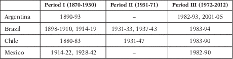
Source: Standard and Poor’s (Borensztein and Panizza Reference Borensztein and Panizza2009).
4. EMPIRICAL RESULTS OF IMPACT OF SOVEREIGN DEBT DEFAULTS ON REAL GDP GROWTH AND OUTPUT LOSSES
In this section, we present the empirical results of the impact of sovereign debt defaults on real GDP growth and on output losses. We first aggregate all data in a pool, which consists of Argentina, Brazil, Chile and Mexico from 1870 to 2012. Then we split the sample in three parts, according to the two most important breaks in the economic history in Latin America since 1870.
4.1 Pooled Data
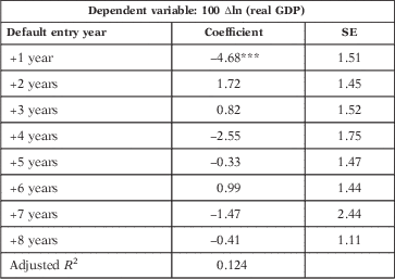
The results for the dummy variable approach are presented in Table 2. On an average, real GDP decreases by 4.7 per cent in the year after the default, and statistically insignificant impact thereafter. We do not find evidence for fixed country effects in the panel. The cumulative impact, measured by Wald tests, is not statistically significant at the 10 per cent level, which means that there is no significant cumulative impact after the 1st year following a default.
TABLE 2 IMPACT OF SOVEREIGN DEBT DEFAULTS ON ECONOMIC GROWTH FOR POOLED DATA (ARGENTINA, BRAZIL, CHILE AND MEXICO; 1870-2012): DUMMY VARIABLE APPROACH
Notes: Control variables: change in government expenses, ratio of government expenses to revenues, population growth, ratio of gross central government debt to GDP, inflation, terms of trade, ratio of exports to imports, polity2, U.S. 3 months T-bill rate, world economic growth (real GDP United States, United Kingdom, Germany and France), U.S. business cycle dummy and changes in commodity prices (cacao, coffee, copper, iron, maize, oil, silver, sugar, tin, zinc); a constant is also included. Variables that are considered potentially endogenous — change in government expenses, ratio of government expenses to revenues, population growth, ratio of gross central government debt to GDP, inflation, terms of trade and ratio of exports to imports — are lagged one period.
We use the White robust estimator, as we find evidence of heteroskedasticity, but not autocorrelation in the panel.
***Significant at 1% levels.
Sources: See text.
We present the results for the complementary measure of the impact — the output loss approach — in Figure 1. Recovery follows 2 years after the default, with two small setbacks, in the 4th and in the 8th year after the default. The output loss is close to zero after 7 years. This means that the actual real GDP almost reaches the real GDP that it would have had if the economy had continued to grow at the pre-crisis growth rate.

FIGURE 1 OUTPUT LOSSES FOR ARGENTINA, BRAZIL, CHILE AND MEXICO, 1870-2012 (POOLED DATA) Notes: The output loss is the percentage difference between the actual real GDP and the real GDP if it had continued the pre-crisis growth. The pre-crisis GDP growth is calculated as the average of the annual growth rate in the 5 years preceding the default entry year.
Sources: See text.
4.2 Zooming in On Three Historical Periods
There have been important breaks in the sample we consider. Each period has substantial different characteristics in terms of institutions, exchange rate regimes, international trade and finance. We distinguish the period 1870-1930, known as the first period of financial globalisation, 1931-1971, also known as the inward-oriented period, and 1972-2012, known as the market reform period or second period of financial globalisation. The two breaks (1931 and 1972) coincide with institutional changes in the global economy, the definitive end of the Gold Standard in 1931 and the end of Bretton Woods in 1972. The standard periodisation in world economic history, where the first globalisation period ends in 1914, is different for Latin American countries. The Great Depression has had a deeper economic impact than the world wars. While WWI was transitionary, the Great Depression was a break with a structural impact — policies became reactive (before policies were passive), gold standard and balanced budgets were replaced by Keynesianism. The outward-looking growth model was replaced by import substitution industrialisation (Diaz-Fuentes Reference Diaz-Fuentes1998). Other authors use the same periodisation as we do, notably Grilli (Reference Grilli2005), and Aiolfi et al. (Reference Aiolfi, Catao and Timmermann2011).
Table 3 shows the impact for each of the three periods. The impact of defaults in period 1870-1930 is significant and negative 1 year after the default (−4.25 per cent), and not significant thereafter. In the period 1931-1971, there is a significant impact of −7.05 per cent 4 years after the default, and of +3.31 per cent 7 years after the default. In the period 1972-2012, we observe a significant impact on economic growth 3 years after the default (−4.00 per cent), and of +1.87 per cent 8 years after the default.
TABLE 3 IMPACT OF SOVEREIGN DEBT DEFAULTS ON ECONOMIC GROWTH, FOR PERIODS 1870-1930, 1931-71 AND 1972-2012 (POOLED DATA): DUMMY VARIABLE APPROACH

Notes: Control variables: see notes in Table 2.
We do not find evidence for fixed country effects in any of the three periods. We use the White estimator, since we find evidence of heteroskedasticity, yet no autocorrelation.
*, **Significant at 10% and 5% levels, respectively.
Sources: See text.
For the cumulative impact of debt default on real GDP growth, we use the Wald test. Table 4 shows that defaults in the 1972-2012 period have a prolonged and negative cumulative impact on economic growth. Up to year 8, the total economic growth is affected by −17.31 per cent.
TABLE 4 CUMULATIVE IMPACT OF SOVEREIGN DEBT DEFAULTS ON ECONOMIC GROWTH, FOR PERIODS 1870-1930, 1931-71 AND 1972-2012 (POOLED DATA): WALD TESTS

Sources and Notes: See Table 2.
As we can see in Figure 2, defaults that occur in the period 1931-1971 have the deepest impact, followed by defaults in the period 1972-2012, while the mildest impact comes from defaults in the period 1870-1930. After the 6th year, the output losses for defaults in the early periods (1870-1930 and 1931-1971) recover fully, while the output losses for defaults in the most recent period (1972-2012) deteriorate further.

FIGURE 2 OUTPUT LOSSES FOR ARGENTINA, BRAZIL, CHILE AND MEXICO, FOR THREE HISTORICAL PERIODS 1870-1930, 1931-71, 1972-2012: POOLED OBSERVATIONS Notes: The output loss is the percentage difference between the actual real GDP and the real GDP if it had continued the pre-crisis growth. The pre-crisis GDP growth is calculated as the average of the annual growth rate in the 5 years preceding the default entry year.
Sources: See text.
An interesting finding is that the defaults in the second period of globalisation (1972-2012) have a deep and long-lasting negative impact on real GDP and the output losses. Bordo et al. (Reference Bordo, Eichengreen, Klingebiel and Martinez-Peria2001) find that currency, banking and twin crises (when currency and banking crises occur simultaneously or when one crisis type triggers another) occur more frequently since 1973 compared to the pre-1913 period, but are not deeper. We find a different result for sovereign debt defaults. The impact is significantly deeper in the post-1972 period than in the pre-1930 period. To provide possible explanations, we turn to the context of the defaults, comparing the defaults in the first globalisation period (1870-1930) with the defaults in the second globalisation period (1972-2012).
Defaults in the period 1870-1930 were more country-specific and not widespread as the defaults in the early 1930s or in the 1980s. Debt was issued in bonds in the international capital markets. Four defaults coincided with low or even negative growth in the run-up to a default (Chile 1880-1883, Brazil 1898-1910, Mexico 1914-1922, Mexico 1928-1942), which implies that the pre-default trend growth was low, and explains the relatively low output losses. In three defaults (Chile 1880-1883, Brazil 1898-1910, Brazil 1914-1919) debt obligations were partially paid, which implied that international capital markets could be re-accessed shortly after the default. With the exception of the Mexico 1928-1942 default, the impact of the default on real GDP growth and the output losses was relatively short-lived. Since the defaults were related to country-specific situations, we briefly describe the six defaults in this period. The default in Chile 1880 coincided with the War of the Pacific (1879-1883). Chile suspended the sinking fund payments, but did pay coupons. In the same year, the price and production of nitrate surged, thus boosting economic growth at record rates until 1882 (Palma Reference Palma2000), which explains the low impact of the default on real GDP. Argentina defaulted in 1890, after a nearly decade-long period of booming economy (Taylor Reference Taylor2005). The country suffered from a sudden stop in capital, a banking and currency crisis, an economic recession, sharp reduction in real wages and the sale of state owned enterprises to foreign investors. The impact was intense, but relatively short-lived (Marichal Reference Marichal1989). Triggered by the drop in coffee prices Brazil defaulted in 1898. It issued a funding loan to pay coupons from 1899 to 1901. Interest payments were made regularly since 1902, but the sinking fund of all the bonds was suspended from 1898 to 1910. The country re-entered the capital markets before it resumed full pay on its debt obligations (Kaminsky and Vega-Garcia Reference Kaminsky and Vega-Garcia2014). In 1914 Brazil defaulted again, while experiencing also a currency and banking crisis. WWI led to a massive international financial crisis, with sudden stops in capital flows, foreign direct investments and international trade (Kaminsky and Vega-Garcia Reference Kaminsky and Vega-Garcia2014; Marichal Reference Marichal1989). Brazil defaulted, but paid interest on its bonds, and maintained access to international capital markets. It implemented an expansive monetary policy, which served to stimulate the economy (Marichal Reference Marichal1989), and thus kept the impact of the default limited. The default in Mexico in 1914-1922 was related to the Revolution War (1910-1920). New borrowing stopped in 1911 (Wynne Reference Wynne1951), and 3 years later the country defaulted. In 1913 the scale of the war increased, and political instability in 1914-1915 was great. A currency and banking crisis coincided with the default. From 1917, the situation in the country started to improve (Knight Reference Knight2000). Because the pre-default trend growth was so low, the impact of the default on real GDP was relatively small. The default of Mexico in 1928-1942 took place when the economy was still fragile after the revolution (Diaz-Fuentes Reference Diaz-Fuentes1998). Mexico suffered from an economic slowdown that started in 1926 and lasted until 1932 (Haber Reference Haber1989). Soon after the default of Mexico in 1928, the Great Depression affected the country heavily, with lower international trade, net capital outflows, lower prices for commodities (Marichal Reference Marichal1989), and banking and currency crises (Reinhart and Rogoff Reference Reinhart and Rogoff2009).
Four out of five defaults in the second globalisation period (1972-2012) occurred in the systemic debt crisis of the 1980s. Most countries experienced high economic growth up to 1981, and assumed high debt levels, in the form of bank loans rather than bonds as in earlier periods. With decreasing commodity prices since 1980, fiscal revenues plunged. After Mexico announced in 1982 that it was unable to meet payment on its foreign debt, interest rates increased sharply, and a sudden stop in commercial bank loans, a reduction in imports (of capital goods and intermediate inputs) and investments seriously affected economic growth (Edwards Reference Edwards1995). The four countries under study also suffered from currency and banking crises. Export revenues had to be destined to service part of the debt obligations. The government expenditures were strongly reduced due to the forced interest payments, while the debt did not diminish (Marichal Reference Marichal2014). Restructuring took a long time, which suggests that restructuring syndicated bank loans is more cumbersome than restructuring international bonds (Borensztein and Panizza Reference Borensztein and Panizza2009). The remainder of the 1980s is known as the «lost decade» for Latin America. There were also differences in the impact of the defaults. While Mexico and Argentina experienced negative or low economic growth until the end of the 1980s, the defaults in Brazil and Chile had a mild impact. Brazil recovered in 1984, when exports surged due to high demand from the United States, while imports decreased (mainly due to the lower oil prices). The trade surplus led to increasing investments, industrial output and economic growth (De Paiva Abreu Reference De Paiva Abreu2008). Chile’s sovereign debt default was actually a consequence of rescuing the bank sector, not from running unsustainable policies or deficit (Edwards Reference Edwards1995).
5. EMPIRICAL RESULTS OF SEVERITY AND DIVERSITY IN THE IMPACT
In this section, we present the empirical results of the diversity in the impact of sovereign debt defaults on output losses. We present our measures for the severity of the impact of each of the fourteen defaults in Section 5.1. additionally, we present a description of the variables that contribute to the diversity of the impact in Section 5.2. It is important to mention that we can only speculate about causality.
5.1 Severity of the impact
Table 5 lists the fourteen sovereign debt defaults, ordered for cumulative output loss during the crisis contraction period.
TABLE 5 SEVERITY OF THE OUTPUT LOSS AND CONTRACTION PERIOD OF SOVEREIGN DEBT DEFAULTS IN ARGENTINA, BRAZIL, CHILE AND MEXICO 1870-2012

Notes: The defaults are ordered based on severity (cumulative output loss). Cumulative output losses are defined to be positive, so a negative coefficient implies a cumulative output gain. The 1880-1883 crises in Chile began an expansion phase, and the economy continued this path after the crisis unfolded. According to our definition there is no contraction period, and therefore no cumulative output loss.Sources: See text.
The debt defaults of Mexico in 1982, Brazil in 1937, Mexico in 1928, Chile in 1931 and Argentina in 1890, the «top 5 deep crises», had a deep impact on the cumulative output loss. In most cases (Mexico in 1982, Brazil in 1937, Chile in 1931 and Argentina in 1890) the default followed a boom period with high GDP growth, followed by a deep international recession, a drop in international trade and a sudden stop in capital flows (Mexico in 1928, 1982, Brazil in 1937 and Chile in 1931). Three of the five deep crises (Mexico in 1928, Chile in 1931 and Brazil in 1937) are related to the 1930s. In this episode the world experienced a deep recession, international trade and commodity prices dropped, and in particular Chile suffered greatly. The international banking crisis in 1931 triggered a series of defaults in Latin America, after capital flew back to European and U.S. banks (de Paiva Abreu 1984; Marichal 1989).
Brazil was an exception: after its default in 1931, it continued to service part of its debt obligations, and was once again lucky in the commodity lottery (Diaz Alejandro Reference Diaz Alejandro2000). Similarly, the «top 5 mild crises» consist of the sovereign debt defaults that had the mildest impact on the cumulative output loss: Chile in 1880, Brazil in 1898, Mexico in 1914, Chile in 1983 and Brazil in 1983. In three cases (Chile in 1880, Brazil in 1898 and Mexico in 1914) the default followed a period of recession, thus having a low pre-default GDP trend. This explains the negative cumulative output loss. The commodity price lottery was favourable for Chile in 1880-1883 and for Brazil in 1983-1994. Chile’s situation in the early 1980s was different than in the rest of Latin America, because it had low sovereign debt. The country defaulted when it took over the external debt from the troubled bank sector in 1983.
5.2 Diversity in The Impact Severity
We use event study graphs à la Kaminsky et al. (Reference Kaminsky, Lizondo and Reinhart1998) to compare the pattern of economic indicators in the run-up to and during default periods with the pattern in tranquil times, which are shown in Figures 3 and 4.

FIGURE 3 PATTERN OF MACROECONOMIC INDICATORS AROUND THE TIME OF THE 1ST YEAR OF A SOVEREIGN DEBT DEFAULT IN ARGENTINA, BRAZIL, CHILE AND MEXICO, 1870-2012 (POOLED DATA): DEEP VS. MILD CRISES Notes: The solid line represents the average of five deep crises (Mexico 1982, Brazil 1937, Mexico 1928, Chile 1931, Argentina 1890). The dotted line represents the average of five mild crises (Chile 1880, Brazil 1898, Mexico 1914, Chile 1983, Brazil 1983) and the intermittent line represents the average in tranquil times.Sources: See text.

FIGURE 4 PATTERN OF WORLD ECONOMIC AND EXTERNAL TRADE INDICATORS AROUND THE TIME OF THE 1ST YEAR OF A SOVEREIGN DEBT DEFAULT IN ARGENTINA, BRAZIL, CHILE AND MEXICO, 1870-2012 (POOLED DATA): DEEP VS. MILD CRISES Notes: The solid line represents the average of five deep crises, the dotted line represents the average of five mild crises and the intermittent line represents the average in tranquil times.Sources: See text.
In Figure 3, we can compare the pattern of deep vs. mild crises for domestic indicators. We observe that deep crises are associated with the expansion phase of the business cycle, high government expenditures and high debt prior to the default, high money (M0) growth, and a more autocratic regime. The four Latin American countries that we investigate experience an equal number of years with autocracy and with democracy. However, the default occurs when there is an autocracy in eleven (out of fourteen) defaults.
Figure 4 presents the pattern of world economic and external indicators. We observe that deep crises occur when international circumstances (interest rate and economic growth) in the run-up to the default are favourable, and adverse in the year of the default and thereafter. High capital mobility is associated with mild crises. In terms of external trade, exports relative to imports remain low until default occurs. When the terms of trade drop, either because of a devaluation of the currency or a relative decrease in export prices, then export competitiveness increases.
Next, we present correlations between the measures of depth and length of each of the defaults and a set of potentially relevant indicators. We only include the thirteen defaults for which we have a measure for the severity and length of the crisis. This means that we exclude the Chile 1880-1883 default. We calculate correlations between the severity measure (depth, respectively length) and a wide range of potentially relevant indicators. We include each indicator in four ways: 1 year before the default, the 3 years average before the default, 1 year after the default entry and 3 years average after the default entry. For exogenous indicators, we also include the contemporaneous values. Since the panel is cross-sectionally narrow with only thirteen default events, we need to be cautious with inferences made.
In Table 6, we show the variables that are correlated with the severity (the cumulative output loss during the contraction period). The level of significance is based on the ratio of critical value to the squared root of the number of observations. A correlation coefficient of 0.456 in absolute terms corresponds to the 90 per cent confidence level
 $$(1.645\!/\!\sqrt {13} )$$
. The domestic indicators (business cycle dummy, real GDP growth, money growth and government expenditure) dominate in terms of the explained variation of the dependent variable. High real GDP growth, an increase in government expenditures and high growth in money aggregates in the years prior to default are associated with a larger cumulative output loss. In other words, when a default follows a period with high economic growth, monetary expansion and pro-cyclical fiscal policy, then the contraction is deeper. This finding fits with boom–bust theories.
$$(1.645\!/\!\sqrt {13} )$$
. The domestic indicators (business cycle dummy, real GDP growth, money growth and government expenditure) dominate in terms of the explained variation of the dependent variable. High real GDP growth, an increase in government expenditures and high growth in money aggregates in the years prior to default are associated with a larger cumulative output loss. In other words, when a default follows a period with high economic growth, monetary expansion and pro-cyclical fiscal policy, then the contraction is deeper. This finding fits with boom–bust theories.
TABLE 6 CORRELATIONS OF SEVERITY OF THE IMPACT OF SOVEREIGN DEFAULTS IN ARGENTINA, BRAZIL, CHILE AND MEXICO, 1870-2012

Sources: See text.
Table 7 shows the variables that are correlated with the length of the contraction period. Global conditions prior to the default dominate. Increasing commodity prices in the 3 years before the default are associated with a longer contraction period. Latin America is a large producer of commodities. Commodity revenues do not only have a direct impact on output, but also an indirect effect, because they sustain government revenues, and export revenues which generate foreign currency. The impact from a decrease in commodity prices is larger when the commodity prices have boomed before the decrease. When world economic growth prior to the default is high, then the length of the contraction period is longer. An increase in the terms of trade in the pre-default year is associated with a longer contraction period. Unfavourable terms of trade point towards an overvalued currency, which increase the probability of a depreciation or devaluation. A depreciation of the currency will increase the debt service obligations in domestic currency, which increases the probability of a sovereign debt default (Bordo and Meissner Reference Bordo and Meissner2007).
TABLE 7 CORRELATIONS OF CONTRACTION PERIOD OF THE IMPACT OF SOVEREIGN DEFAULTS IN ARGENTINA, BRAZIL, CHILE AND MEXICO, 1870-2012

Sources: See text.
6. CONCLUSION
In this paper, we analyse the impact of sovereign debt defaults on real GDP growth for four Latin American countries: Argentina, Brazil, Chile and Mexico. These countries have experienced fourteen sovereign defaults from 1870 to 2012.
To measure the impact of sovereign debt defaults on real GDP growth and the output losses we use the dummy approach and output loss approach. We observe a negative impact of a default on real GDP growth in the 1st year after the default entry, and no significant impact thereafter. While Bordo et al. (Reference Bordo, Eichengreen, Klingebiel and Martinez-Peria2001) find that currency, banking and twin crises occur more frequently but are not more severe after 1970, we find a different result for sovereign debt defaults: defaults in the period 1972-2012 have a deeper and longer lasting impact than defaults in the period 1870-1930. On the one hand, this can be attributed to the 1980s Latin American debt crisis, in particular for Mexico, Argentina and to a lesser extent Brazil. During the long renegotiation process, the countries had no access to capital and governments were forced to use a significant part of the fiscal budget and export revenues to service debts. Contractions in imports of capital goods and intermediate inputs, and a sharp fall in investments affected growth. For Brazil, the situation was less dramatic since it could take advantage of higher exports and lower import prices. On the other hand, defaults in the period 1870-1930 led to relatively short periods of reduced access to capital markets, and most countries were able to increase exports, which supported financial recovery.
To analyse the diverse impact of defaults on output losses, we investigate a possible close relation between the severity of the impact and economic, financial, political and global conditions around the time of default. We find that the depth of a default, measured as the cumulative output loss, is correlated with domestic indicators, primarily government expenditures, real GDP growth and money growth prior to the default. The contraction period, measured as the time it takes from the year of the default to reach the trough of the business cycle, is associated mainly mostly with international variables: high economic growth rates in the world in the run-up to a default and high pre-default commodity price increases are associated with defaults with a long contraction period. We also find that deep crises are associated with favourable global circumstances (low interest rates, high world growth) in the run-up to a default and unfavourable global circumstances in the aftermath of a default. Capital mobility is low in deep crises, and deep crises are associated with more autocratic regimes. Our findings coincide partly with Cerro and Meloni (Reference Cerro and Meloni2013), who find that very deep currency crises in Argentina are associated with growing government expenditures, high debt levels and unfavourable external circumstances, including high terms of trade, which indicate a possibly overvalued currency. Our findings fit in with the boom–bust theory, sudden stop models and the political economy theory which relates commodity prices and government expenditures to the political system. Our finding that the depth of the impact depends on domestic conditions in the run-up to the default may be useful for policy makers.
Latin America has a long history of recurrent debt defaults. Our findings support the view that procyclical fiscal policy and reliance on commodities have made the countries vulnerable to unfavourable international developments (low economic growth, high interest rates and decreasing commodity prices). In the most recent commodity boom (2002-2007) most Latin American countries have used the extra revenues to reduce debt positions, to increase foreign reserves and to maintain the fiscal balance (Kacef and Lopez-Monti Reference Kacef and Lopez-Monti2010). This has allowed Brazil and Chile to follow countercyclical fiscal policy during the Global Financial Crisis that hit emerging countries in the fall of 2008. Although the region was hit hard by the crisis, it did not lead to financial crises other than a currency crisis in the region, contrary to past global crises.


