


1. Introduction
Understanding the kinematics and mechanics of the flow of granular materials is of considerable importance, as they are encountered in a wide variety of industrial and natural processes. Though a variety of complicating factors, such as intergrain cohesion and complex grain shape, may be present in practical systems, the limit of non-cohesive and nearly spherical grains is sufficiently prevalent and challenging that it has been investigated in numerous previous studies. For such systems, the relative importance of grain inertia is one of the factors that determine the kinematics and rheology. It is quantified by the dimensionless Savage number (Savage & Hutter Reference Savage and Hutter1989)  ${Sa}$, or equivalently the inertial number ${\mathcal {I}}$ (GDR MiDi 2004), defined as
 \begin{equation} {Sa} =\frac{\displaystyle \rho_{{p}} d_{{p}}^2 \dot{\gamma}^2}{\displaystyle N} = {\mathcal{I}}^2 , \end{equation}
where  $\rho _{{p}}$ and $d_{{p}}$ are the density and size of the particles, $\dot {\gamma }$ is the nominal strain rate and $N$ is a stress scale. The numerator in (1.1) is proportional to the stress arising from inertial collisions between grains; ${Sa}$ is therefore a measure of the contribution of grain inertia to the stress. When ${Sa} \ll 1$, grain inertia is of little consequence and stress transmission is primarily via sustained grain contacts wherein Coulomb friction plays an important role. This regime is commonly referred to as slow flow; it is operational in many terrestrial flows where gravity consolidates the medium to a dense enough state that contacts between particles are abiding – examples are flow through hoppers and silos, conveying of mineral ores through screw conveyors, and in earthmoving operations. In the opposite limiting regime of ${Sa} \sim 1$, grains interact by short term collisions, and momentum transport is due to the inertial impulse during collisions; it is operational in avalanches, flow down inclined chutes, and fluidized beds. Continuum models for the above limiting regimes are based on extensions of soil and metal plasticity for the former, and the kinetic theory of gases for the latter. The range of ${Sa}$ between these limiting regimes is the so-called intermediate regime, which is not very well understood and is an active area of research.
Our attention in this paper is restricted to the slow flow of dense non-cohesive granular materials. Experimental observations in this regime show the following characteristic features: (i) the stress is independent (or very weakly dependent) on the magnitude of the deformation rate (Wieghardt Reference Wieghardt1975; Rao & Nott Reference Rao and Nott2008); (ii) shear is typically confined to narrow shear layers (Natarajan, Hunt & Taylor Reference Natarajan, Hunt and Taylor1995; Losert et al. Reference Losert, Bocquet, Lubensky and Gollub2000; Ananda, Moka & Nott Reference Ananda, Moka and Nott2008); and (iii) dilatancy, or volume deformation caused by shear deformation (Reynolds Reference Reynolds1885; Desrues et al. Reference Desrues, Chambon, Mokni and Mazerolle1996; Kabla & Senden Reference Kabla and Senden2009). Of these, dilatancy is perhaps the most distinctive feature – while rate independence may be thought of as an extreme example of a shear thinning fluid, and shear banding is observed in a variety of complex fluids (foams, emulsions and nematic liquid crystals being a few examples), dilatancy has no analogue in fluids.
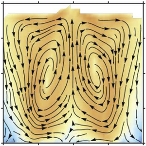
Until recently, dilatancy was thought to be important only during flow initiation within the shear layer. It was generally believed to have little consequence on the kinematics and rheology in sustained flow – indeed almost all rheological models for slow granular flow treat the medium as incompressible. The recent study of Krishnaraj & Nott (Reference Krishnaraj and Nott2016) showed that its effect can extend well beyond the shear layer; they demonstrated the occurrence of a dilatancy-driven steady secondary flow in the form of a system-spanning vortex in the velocity gradient-gravity plane in a cylindrical Couette device. A sample result from Krishnaraj & Nott (Reference Krishnaraj and Nott2016) is reproduced in figure 1 to illustrate their findings. The primary flow in this geometry is the azimuthal velocity field  $u_\theta (r)$ that decays roughly exponentially with distance from the inner cylinder. Dilatancy in the shear layer requires depletion of grains, resulting in a radial outward and upward flow of particles (figure 1b). Simultaneously, particles percolate down the region of low density near the inner cylinder due to gravity, and at steady state the balance between these two effects results in a system-spanning vortex (figure 1c). They found no secondary flow in the absence of gravity, which led them to the conclusion that dilatancy and gravity are necessary ingredients for the secondary vortex, provided the velocity gradient (of the primary flow) and gravity directions are not collinear. Krishnaraj & Nott (Reference Krishnaraj and Nott2016) further showed that the secondary flow explains the puzzling rheological anomaly observed by Mehandia, Gutam & Nott (Reference Mehandia, Gutam and Nott2012) and Gutam, Mehandia & Nott (Reference Gutam, Mehandia and Nott2013) that all components of the stress on the outer cylinder in a cylindrical Couette cell were found to rise exponentially with depth. Thus, though the secondary flow is weak, the rate independence of the stress in the slow flow regime implies that it can leave a large rheological signature.

Figure 1. Dilatancy-driven secondary flow in a cylindrical Couette device. The figures are adapted from Krishnaraj & Nott (Reference Krishnaraj and Nott2016). (a) Schematic of the cylindrical Couette device. (b) Streamlines of the secondary flow at early stages of shear, after a  $3.4^\circ$ rotation of the inner cylinder. (c) The secondary flow at steady state, showing a system-spanning vortex. The colours in panels (b,c) indicate $\log _{10} s$, where $s \equiv (u_r^2 + u_y^2)^{1/2}$ is the speed of the secondary flow.
We emphasize that the phrases ‘primary flow’ and ‘secondary flow’ are used throughout this paper differently from their standard usage to describe fluid instabilities. By primary flow, we mean the flow in the expected direction, parallel to the moving boundary. By secondary flow, we refer to the flow that is in the plane of the velocity gradient (of the primary flow) and gravity. In the cylindrical Couette device, the primary flow is in the  $\theta$ direction, and the secondary flow is in the $r$–
$r$– $y$ plane (figure 1c). In particular, we note that the secondary flow does not appear to arise as a result of an instability of the primary flow, as is typically the case in fluids – all the evidence we have so far indicates that the secondary flow is an inherent aspect of the flow field, no matter how low the shear rate.
The work reported in this paper was motivated by the question: How general is the dilatancy-driven secondary flow observed by Krishnaraj & Nott (Reference Krishnaraj and Nott2016)? To answer it, we investigate the flow in a split-bottom shear cell, in which the base of the container holding the granular material is split into two parts, one of which moves and the other (along with the vertical walls) is held stationary. This device was first used by Fenistein, van de Meent & van Hecke (Reference Fenistein, van de Meent and van Hecke2004) to demonstrate the possibility of obtaining ‘wide shear bands’ in granular materials, or shear layers wider than what is typically obtained near a moving boundary. However, that is not the property of interest for our study. Rather, it is the feature that the primary velocity field is much more complex than in a cylindrical Couette device, as the direction of the velocity gradient (of the primary flow) varies from nearly vertical above the symmetry axis to nearly horizontal across the fan-shaped shear layers above the split. Moreover, the primary flow changes character quite substantially as the fill height is increased (Cheng et al. Reference Cheng, Lechman, Fernandez-Barbero, Grest, Jaeger, Karczmar, Möbius and Nagel2006; Fenistein, van de Meent & van Hecke Reference Fenistein, van de Meent and van Hecke2006; Dijksman & van Hecke Reference Dijksman and van Hecke2010). We show that there is indeed a dilatancy-driven secondary flow for all fill heights (within the range explored), but it is more complex than in the cylindrical Couette device. Nevertheless, some key features of the secondary vortices remain the same: an upward and lateral flow driven by dilatancy, and a downward flow through the dilated shear layers. Most of the results presented are obtained computationally from particle dynamics simulations. The computations are complemented by video imaging experiments to determine the radial velocity profile on the free surface. The experimental measurements are found to be in good qualitative agreement with the velocity profiles obtained from the computations.
2. Computational and experimental methods
The geometry of interest in this study is a split-bottom shear cell, shown in figure 2. It is a container with vertical sidewalls whose base is split into two parts, one of which is set in motion. In our computational studies, we first consider a container of rectangular cross-section (figure 2a) as it is computationally less demanding, and also allows us to easily illustrate the main features of the secondary flow. In this cell, the middle section of the base translates with constant velocity  $V_w$ and the rest of the base and the sidewalls are held stationary. The front and back faces of the cell ( $z = 0, L$) are periodic boundaries that impose no resistance to flow. To understand the effect of the sidewalls on the flow, we also consider the simpler case where the left and right vertical walls ( $x = 0, 2W$) are periodic boundaries. We then consider a cylindrical cell (figure 2b), wherein the central core of the base is rotated at constant angular velocity $\varOmega _w$ and all other boundaries are held stationary.

Figure 2. Schematics of the (a) rectangular and (b) cylindrical split-bottom shear cells. The cells are filled to a height  $H$ by ‘raining’ the particles from above. In the rectangular device, the middle section of the base of width $W$ translates with a velocity $V_w$ in the $z$ direction, and in the cylindrical device, the central core of radius $R_i$ rotates with angular velocity $\varOmega _w$. (c) Schematic of the interaction model in the discrete element method (DEM). The overlap $\delta$ is exaggerated for clarity.
The granular material is composed of spherical particles of mean diameter  $d_p$ – to avoid crystallization, a mixture of sizes $0.9\, d_p$, $d_p$ and $1.1\, d_p$ with number fractions $0.3$, $0.4$ and $0.3$, respectively, is used. The base and sidewalls of the shear cell are composed of particles of diameter $d_p$ arranged in a triangular lattice that are either static (stationary walls) or translated/rotated as a rigid body (moving section of the base). For the rectangular shear cell, the half-width $W$ and depth $L$ of the base are $40\, d_p$. For the cylindrical shear cell, the radii of the rotating base and container are $R_i = 37\, d_p$ and $R_o = 50\, d_p$. The shear cell is filled by ‘raining’ particles from a reservoir above the system under gravity until the required fill height is reached. The height $H$ that is reported is the maximum height reached by the material at steady state – we have considered fill heights, $H = 35\, d_p$, $45\, d_p$ and $55\, d_p$ for the reasons given in § 3. As our interest is in the slow flow regime, we choose the velocities of the moving walls such that the Savage or inertial numbers are small. Taking the stress scale $N$ to be the hydrostatic head $\rho g H$, and the nominal shear rate $\dot {\gamma }$ as $V_w/W$, the Savage number $\mathit {Sa}$ in the simulations is in the range $8.2 \times 10^{-7}$ to $1.8 \times 10^{-5}$ ( ${\mathcal {I}}$ is in the range $9 \times 10^{-4}$ to $4.2 \times 10^{-3}$). For the cylindrical cell, $V_w \equiv \varOmega _w R_i$ is the velocity scale, whence the nominal shear rate is $\dot {\gamma } = \varOmega _w$. To confirm that this is low enough, we have conducted a simulation for the smallest fill height with a wall velocity lower by a factor of 10 ( ${Sa}$ lower by a factor of 100), and found no qualitative difference in the velocity and density fields. To explore the effect of particle inertia, we have conducted one simulation in the cylindrical cell in which rotation speed of the base was increased by a factor of 100, yielding a Savage number of ${Sa} = 8.2 \times 10^{-3}$ ( ${\mathcal {I}} = 9 \times 10^{-2}$).
The computations are carried out using the DEM, a widely used tool for simulating granular statics and flow. As it is described in numerous papers, we provide only a brief outline of the method here. In DEM, particles are treated as deformable during interactions, but rather than calculate their deformation in detail, they are allowed to overlap. The interaction forces are written in terms of the overlap and its time rate of change (Cundall & Strack Reference Cundall and Strack1979; Walton & Braun Reference Walton and Braun1986; Silbert et al. Reference Silbert, Ertas, Grest, Halsey, Levine and Plimpton2001). The normal and tangential forces have elastic and viscous components, and the tangential force incorporates an additional Coulomb slider to capture rate-independent friction (figure 2c). Considering the contact of particles  $i$ and $j$ centred at position vectors $\boldsymbol {r}_i$ and $\boldsymbol {r}_j$, the normal and tangential forces on particle $i$ are
 \begin{gather} \boldsymbol{F}_n = k_n \delta \boldsymbol{n}-m_{{eff}} \gamma_n \boldsymbol{v}_n, \end{gather}
 \begin{gather}\boldsymbol{F}_t = \begin{cases} -k_t \Delta \boldsymbol{s} - m_{{eff}} \gamma_t \boldsymbol{v}_t, & \text{if}\ |F_n/F_t| < \mu ,\\ -\mu|F_n| \dfrac{\boldsymbol{v}_t}{|\boldsymbol{v}_t|}, & \text{otherwise}. \end{cases} \end{gather}
Here,  $\boldsymbol {n}$ is the unit normal at the point of contact pointing towards the centre of $i$,
$i$,  $\delta \equiv \frac {1}{2} (d_i + d_j) - |\boldsymbol {r}_i - \boldsymbol {r}_j |$ is the overlap, $\Delta \boldsymbol {s}$ is the tangential displacement post contact, $\boldsymbol {v}_n$ and $\boldsymbol {v}_t$ are the normal and tangential relative velocities at contact, and $m_{{eff}} \equiv (1/m_i+1/m_j)^{-1}$ is the effective mass. The interaction parameters are the normal and tangential spring constants $k_n$ and $k_t$, the corresponding damping coefficients $\gamma _n$ and $\gamma _t$, and the Coulomb friction coefficient $\mu$. Their values are taken from Krishnaraj & Nott (Reference Krishnaraj and Nott2016), namely $k_n = 10^6\, m_p g/d_p$, $k_t = \frac {2}{7} k_n$, $\gamma _n = 317 \sqrt {g/d_p}$, $\gamma _t = \frac {1}{2} \gamma _n$ and $\mu = 0.5$, as they were found to be appropriate for hard spheres such as glass beads. Here $m_p$ is the mass of a particle of diameter $d_p$. The position of each particle is tracked by integrating Newton's second law in time. The time step used for numerical integration is $t_{{coll}}/50$, where $t_{{coll}} = {\rm \pi}(2 k_n/m_p - \gamma _n^2/4)^{-1/2}$ is the duration of a collision between grains (Silbert et al. Reference Silbert, Ertas, Grest, Halsey, Levine and Plimpton2001).
The continuum density and velocity fields were calculated by averaging particle quantities over suitably chosen bins for a sufficiently long period of time. For the rectangular cell, the bins were square cuboids of depth  $L$ and cross-sectional area in the range 1.21–3 $\,d_p^2$, and for the cylindrical cell they were toroids of square cross-sectional area 1.21 $d_p^2$. The simulations were run until the velocity $u_z$ averaged in time windows of $5/\dot {\gamma }$ changed by less than 0.3 % in every bin, which was taken to be the steady state. Small fluctuations in the secondary velocity are seen between adjacent time windows at steady state, but the average change over all bins was less than 2.4 %. To ensure that the flow at steady state is fully developed, the shear cell was divided into two halves in the flow direction and the velocity fields in them compared – they were found to be nearly indistinguishable.
In our experiments, a cylindrical split-bottom device with dimensions diameter  $R_i = 37\ \mbox {mm}$, $R_o = 50\ \mbox {mm}$ was constructed from aluminium, and the base was coated with sandpaper. The system is filled with glass beads of mean diameter $d_p = 1\ \mbox {mm}$ and density $\rho _p = 2500\ \mbox {kg}\ \mbox {m}^{-3}$; the height increases slightly as the material dilates during shear, and the steady state height at the cylinder is reported as the fill height $H$. The base was rotated at 1 rpm, for which ${Sa} \approx 10^{-6}$. The flow on the free surface was imaged using a video camera (Phantom C110) mounted above the system such that the field of view spans the entire bed surface. The base was rotated for 30 revolutions to ensure that steady state was reached, after which the surface was imaged at $70\ \textrm {frames}\ \textrm {s}^{-1}$. The tangential and radial velocities were determined using a particle image velocimetry module in MATLAB (Thielicke & Stamhuis Reference Thielicke and Stamhuis2014).
3. Results for the rectangular shear cell
The features of the primary and secondary flows are best illustrated by first considering the shear cell of rectangular cross-section. The expected flow is in the  $z$ direction – this is the primary flow. Shear originates at the split and permeates to distances in the $x$ and $y$ directions that depend on the fill height. However, shear is accompanied by dilation, which causes an initially dense material to expand. As shown by Krishnaraj & Nott (Reference Krishnaraj and Nott2016), this leads to a secondary flow in the velocity gradient-gravity plane – their sample results reproduced in figure 1 are a useful reference point to compare our findings with. As the geometry and boundary conditions are symmetric about the plane $x = 0.5$, we expect the velocity and density fields to exhibit the same symmetry.
3.1. Rigid sidewalls
We first consider a rectangular split-bottom shear cell with rigid, frictional sidewalls. The steady state primary velocity fields  $u_z(x,y)$ for the three fill heights are shown in figure 3. For the smallest fill height $H = 0.88 {W}$, shear propagates all the way to the free surface, with the contours of constant $u_z$ fanning out above the two splits and the width of the shear layer increasing with $y$ (figure 3a). The velocity gradient within the fan is predominantly in the $x$ direction. In addition, there is a region of relatively weak shear in the dome-shaped region above the moving base. For the largest fill height $H = 1.38 W$, the contours of constant $u_z$ connect one split to the other, forming a dome-shaped shear zone over the moving base (figure 3c). In this case, $u_z$ has gradients in the $x$ and $y$ directions, and it decays rapidly with $y$. For the fill height of $1.13 W$, the nature of the primary velocity field is intermediate between the other two cases: we see a dome-shaped shear layer over the base as well as weak fan-shaped shear layers over the two splits (figure 3b). These three heights suffice to describe qualitatively the entire range of primary flow seen for all fill heights. The observed transitions between shallow, intermediate and deep systems are consistent with those observed by previous studies (Cheng et al. Reference Cheng, Lechman, Fernandez-Barbero, Grest, Jaeger, Karczmar, Möbius and Nagel2006; Fenistein et al. Reference Fenistein, van de Meent and van Hecke2006).

Figure 3. The primary flow obtained from DEM simulations of the rectangular split-bottom shear cell for fill heights  $H$ of (a) $0.88 { W}$, (b) $1.13 { W}$ and (c) $1.38 {W}$. The colours indicate the scaled velocity $u_z/V_w$, and the lines are contours of constant velocity in steps of $0.091$.
The different regions of shear for the three fill heights result in correspondingly different density fields. Figure 4(a–c) show the steady state density field for the three cases in terms of the particle volume fraction  $\phi (x,y)$. For the smallest fill height, $\phi$ is low in the fan-like shear layers due to strong dilation; dilation is also evident in the relatively weakly sheared dome-shaped region over the moving base (see figure 4a). As the fill height increases, the extent of dilation decreases over the fan-line shear layers and increases in the dome-shaped shearing region over the moving base (see figure 4b,c). Thus, the dilated regions of low density largely coincide with the shearing regions in all the cases.

Figure 4. Volume fraction and secondary velocity fields in the rectangular shear cell. (a–c) Colour maps of the particle volume fraction  $\phi$ for fill heights $H$ of (a) $0.88 W$, (b) $1.13 W$ and (c) $1.38 W$. Regions of very low $\phi$ are coloured white – we have chosen a cutoff of 0.4, but any cutoff less than ${\approx } 0.55$ yields the same result. (d–f) Streamlines of the secondary flow for the same fill heights as in figures above. The colours indicate the speed of the secondary flow $s \equiv (u_x^2 + u_y^2)^{1/2}/V_w$ on a logarithmic scale.
As in the cylindrical Couette cell of Krishnaraj & Nott (Reference Krishnaraj and Nott2016) (see figure 1b), a secondary flow in the form of steady vortices in the plane of the velocity gradient (of the primary flow) and gravity is observed for all fill heights. Streamlines constructed by interpolation of the local velocity vectors are shown in figure 4(d–f), with the background colour indicating the logarithm of the speed  $s \equiv (u_x^2 + u_y^2)^{1/2} / V_w$ of the secondary flow. For the smallest fill height, we see two counter-rotating vortices (figure 4d) that span the entire cell. Particles rise around the centre of the moving plate and fall through the dilated shear layer over the splits. For the intermediate and large fill heights, there are four vortices, two in each half of the shear cell – the upper vortices are larger and their sense is the same as in the shallow system. The lower vortices have the opposite sense: particles rise over the splits and fall through the dilated region over the moving base. The strength of the vortices decreases sharply with increasing $H$. We note that the streamlines shown in figure 4(d–f) are obtained by averaging over a long period of time, as there are considerable fluctuations in the secondary flow, particularly at the intermediate and largest fill heights. The vortices seen in the figures are therefore only statistically steady. However, the time-averaged flow at the statistically steady state is reproducible over repeated runs. Supplementary movie 1 shows an animation of the motion of particles in the $x$–
$x$– $y$ plane for the simulation with $H = 0.88 W$ – despite the fluctuations in particle motion, the formation of the secondary vortices is clearly discernible. The $x$ and $y$ axes in figures 3 and 4 are scaled by $2W$ and $H$, respectively, to obtain plots of the same size. To clearly convey the aspect ratio of the shear cells and size of the vortices, the figures are presented with both axes scaled by $2W$ in supplementary figure S1, which is available at https://doi.org/10.1017/jfm.2020.1029.
Several features of the velocity and density fields merit discussion. The form of the primary flow for the first two fill heights is quite similar to what is observed in experiments (Cheng et al. Reference Cheng, Lechman, Fernandez-Barbero, Grest, Jaeger, Karczmar, Möbius and Nagel2006) and our simulations (see § 4) of a cylindrical split-bottom cell. The rectangular shear cell yields a clearer picture of the flow, due to the absence of the curvature-induced bending of the shear layer. The weakly dilated regions seen for the two larger fill heights (figure 4b,c) are indeed regions of shear – this is not apparent from the colour map of the primary velocity field (figure 3b,c), but it is seen clearly in figure 5(a), which shows  $u_z$ on a logarithmic scale as a function of $x$ for two heights. It is evident that there is an exponential decay of the velocity all the way up to the sidewalls. Comparison of figures 5(a) and 5(b) reveals that the secondary flow is much slower than the primary – except close to the sidewalls, $s$ is smaller than $u_z/V_w$ by approximately a factor of $\sim$100. Nevertheless, as already stated, the secondary flow is robust and reproducible. A close inspection of figure 4(d–f) may give the impression that the streamlines spiral inwards. This is an artefact of discretization errors in computing the continuum velocity field and errors in interpolation. As discussed in § 4, if we determine the stream function and draw streamlines as contours of constant stream function, we get near-perfect circulations for the smallest fill height (see figure 9); for larger fill heights, computation of the stream function too is susceptible discretization and interpolation errors. Further discussion on how the system chooses the form of the primary and secondary flow fields for each fill height and other aspects of the kinematics is given in § 5.

Figure 5. Magnitude of the scaled (a) primary and (b) secondary velocities as a function of  $x$ at two heights, $y = 0.25\, H$ (dashed lines) and $y = 0.75\, H$ (solid lines) in the rectangular shear cell.
We note that Krishnaraj & Nott (Reference Krishnaraj and Nott2016) found no secondary flow in the absence of gravity in the cylindrical Couette cell. To assess the effect of gravity in the split bottom cell, we conducted a simulation wherein the grains are ‘rained’ into the shear cell under gravity to a fill height  $H = 0.88 W$, after which a rigid, frictionless upper plate is fixed at a height $1\,d_{{p}}$ above the free surface. Gravity is then turned off, shear initiated, and the system allowed to reach steady state. The results are shown in figure 6, where it is clear that the primary flow is very different from that in the presence of gravity (figure 3a). While shear is confined to the shallow dome-shaped region in the absence of gravity, there is a fan-like shear layer that propagates all the way to the free surface in the presence of gravity. The density field in figure 6(b) also differs substantially from that in the presence of gravity (figure 4a) – dilation is confined to the dome over the splits, and the material beyond is compacted. Importantly, there is no secondary flow at steady state in the absence of gravity, confirming the hypothesis of Krishnaraj & Nott (Reference Krishnaraj and Nott2016) that the vortices are a result of the combined effect of dilatancy and gravity. Further discussion on how gravity affects the evolution of the velocity and density fields is given in § 5.


Ries, Wolf & Unger (Reference Ries, Wolf and Unger2007) conducted DEM simulations of the flow of perfectly inelastic grains in a split-bottom cell wherein each sidewall moves with the same velocity as the section of the split base to which it is joined. Though the geometry of their shear cell and the nature of grain interactions differ from ours, it is notable that in the absence of gravity they found transient secondary vortices that vanish at steady state, in agreement with our hypothesis. Ries et al. did not study the secondary flow in the presence of gravity. Transient vortices were also observed by Rognon, Miller & Einav (Reference Rognon, Miller and Einav2015) when they sheared a two-dimensional assembly of disks resting on a smooth surface.
3.2. Periodic sidewalls
It is of interest to understand in what way the sidewalls impede and modulate the flow. For this, we replace the rigid, frictional sidewalls with periodic boundaries, about which the velocity and volume fraction fields are symmetric. As the gradients of the velocity and volume fraction normal to the periodic boundaries must vanish, the symmetry about  $x = W$ and invariance with respect to the Galilean shift $u_z \to u_z - V_w$, accompanied by translation of the origin by $W$ along the $x$ axis and reversal of the $z$ and $x$ axes, implies that the planes $x = 0$ and $x = 2W$ are identical to $x = W$. The results of simulations for the same fill heights as in the shear cell with walls are displayed in figure 7 (see also supplementary figure S2).

Figure 7. Results of the DEM simulations for a rectangular shear cell with periodic sidewalls. The figures in each column are for the same fill height  $H$. (a–c) The primary flow for fill heights $H$ of $0.88 W$, $1.13 W$ and $1.38 W$. The colours indicate the scaled velocity $u_z/V_w$, and the solid lines are contours of constant velocity in steps of $0.091$. The dashed line in panel (b) is a contour for $u_z/V_w = 0.6$. (d–f) Colour maps of the particle volume fraction $\phi$. (g–i) Streamlines of the secondary flow. The colours indicate the speed of the secondary flow $s \equiv (u_x^2 + u_y^2)^{1/2}/V_w$ on a logarithmic scale.
The primary velocity field differs mainly in two respects from that observed in figure 3 for the case with sidewalls: the first is the presence of dome-shaped shear layers over the stationary sections of the base for all the fill heights. The second is that  $u_z$ far above the stationary base is higher, and for the largest fill height it asymptotes to $V_w/2$ (while in figure 3c it asymptotes to 0). The other features of the primary flow, such as the fan-shaped shear zones over the splits transitioning to the dome-shaped shear zone over the moving base with increasing $H$ remain largely unchanged. Expectedly, shear over the stationary sections of the base is accompanied by dilation, leading to low-density regions therein (figure 7d–f). For the smallest fill height, this leads to additional vortices in the secondary flow wherein particle rise at the periphery and fall into the fan-shaped dilated region over the splits (figure 7g). The absence of the sidewalls has a bigger effect on the upper vortices for the larger fill heights: they are much smaller in extent for $H = 1.13 W$ and vanish altogether for $H = 1.38 W$. For the latter case, the streamlines in figure 7(i) indicate continuous dilation of the bed, but this obviously cannot continue indefinitely – slow dilation is punctuated by fast compaction events (not shown), and the process appears to repeat itself indefinitely. A transverse flow or drift to the right is seen in figure 7(i), which we believe is due to slight asymmetry in packing that occurs spontaneously – the direction of drift depends on the averaging time, as flow in both directions is observed during the simulation. However, the magnitude of the transverse velocity is very small.
It is thus clear that while the base drives shear, the impenetrable, frictional sidewalls do play a role in determining the shape of the dilated regions and the form of the secondary flow. However, the broad features of the secondary flow and their relation to the form of the primary flow remain the same, regardless of the nature of the sidewalls. Supplementary movie 2 shows an animation of the motion of particles in the  $x$–
$x$– $y$ plane for the simulation with periodic sidewalls with $H = 1.13 W$, where the formation of the secondary vortices is clearly observable.
4. Results for the cylindrical shear cell
We have established the existence of a dilatancy-driven secondary flow in split-bottom shear cells using the rectangular geometry. Nevertheless, verification by experiment is desirable, thereby requiring simulation of a cylindrical shear cell. Apart from allowing experimental verification, the curvilinear primary flow  $u_\theta (r,z)$ in a cylindrical cell introduces some changes in the kinematics that merit study. Nevertheless, we shall see that the essential features of the flow and density fields are largely similar to those in a rectangular cell.
We consider fill heights  $H = 0.43$, 0.73 and $1.27 \, R_i$ (16 , 27 and $47\, d_p$, respectively) as representative examples of small, intermediate and large $H$. Figure 8 shows the results for all three fill heights (see also supplementary figure S3). The form of the primary flow (figure 8a–c), given in terms of $\omega \equiv u_\theta /r$, is quite similar to that determined experimentally by Cheng et al. (Reference Cheng, Lechman, Fernandez-Barbero, Grest, Jaeger, Karczmar, Möbius and Nagel2006) using magnetic resonance imaging, and less accurately by Fenistein et al. (Reference Fenistein, van de Meent and van Hecke2006) who inferred the bulk motion by removing particles above different heights $z$ and inspecting the pattern formed by coloured tracers. For the smallest fill height $H = 0.43\, R_i$, we see a core undergoing solid body rotation, and shear occurring predominantly in the fan-shaped shear layer. For the largest fill height $H = 1.27\, R_i$ shear is primarily in the dome-shaped region above the rotating portion of the base. For $H = 0.73\, R_i$ the primary flow is intermediate between the other two, with the dome-shaped shear zone smoothly merging into a broad fan-shaped shear zone. Thus, the primary velocity field qualitatively resembles the right half ( $0.5 \leqslant x/(2W) \leqslant 1$) of the plots for the rectangular cell shown in figure 3. The density fields (figure 8d–f) conform to expectation, showing dilation in the shearing region and compaction far from it.

Figure 8. Results of the DEM simulations for the cylindrical shear cell. The figures in each column are for the same fill height  $H$. (a–c) The primary flow for fill heights $H$ of $0.43 \, R_i$, $0.73 \, R_i$ and $1.27 \, R_i$. The colours indicate the scaled angular velocity $\omega /\varOmega _w$, and the lines are contours of constant angular velocity in steps of 0.091. (d–f) Colour maps of the particle volume fraction $\phi$. (g–i) Streamlines of the secondary flow. The colours indicate the speed of the secondary flow $s \equiv (u_r^2 + u_y^2)^{1/2}/V_w$ on a logarithmic scale.
The secondary velocity field exhibits a few qualitative differences with that in the rectangular cell. For all the fill heights, there are two adjacent counter-rotating vortices. The vortices span the height of the shear cell for  $H = 0.43$ and $0.73\, R_i$, but shrink considerably as a fraction of the fill height for $H = 1.27\, R_i$. For the largest fill height, figure 8(i) shows material dilating slowly over the vortices, but as in the rectangular cell with periodic sidewalls (figure 7i), this slow dilation is punctuated by fast compaction events. The sense of the vortices is such that the downflow is roughly over the split in the outer vortex and near the centre for the inner vortex. As already mentioned, there is considerable fluctuation in the secondary flow, and the streamlines shown in figure 8(g–i) are long-time averages. Even then, the outer vortex in figure 8(g) does not seem well formed. To show that it is indeed a vortex, we define the stream function $\psi$ such that
 \begin{equation} \phi u_r = \frac{\partial \psi}{\partial y}, \quad \phi u_y = -\frac{\partial \psi}{\partial r}, \end{equation}
which identically satisfies the steady state mass conservation. For the rectangular shear cell,  $r$ is replaced by $x$. The stream function was determined by numerically integrating (4.1a,b) using the discretized array of $u_r$, $u_z$ and $\phi$; the streamlines then are contours of constant $\psi$. The results for the smallest fill heights of the rectangular and cylindrical cells are shown in figure 9(a,b), which are to be compared with figures 4(d) and 8(g), respectively. It is clear that the streamlines of the secondary flow are indeed closed circulations. However, computation of $\psi$ is susceptible to the same errors as the interpolated velocity fields, rendering the results much noisier and therefore not useful for the larger fill heights.

Figure 9. Streamlines of the secondary flow determined as contours of constant stream function  $\psi$, defined in (4.1a,b). (a) Contours of constant $\psi$ in a rectangular shear cell with frictional sidewalls for fill height $H = 0.88 W$. (b) Contours of constant $\psi$ in a cylindrical shear cell for $H = 0.43\, R_i$.
The only other studies that we are aware of where such a secondary flow has been observed are those of Wortel et al. (Reference Wortel, Börzsönyi, Somfai, Wegner, Szabó, Stannarius and van Hecke2015) and Fischer et al. (Reference Fischer, Börzsönyi, Nasato, Pöschel and Stannarius2016) for slender rods, where the secondary flow results in the formation of a heap, or a curved free surface, centred at the axis of rotation. Interestingly, they found the secondary flow to be entirely absent for spherical particles, and argue that the secondary flow is caused by a misalignment of the orientation of particles with the direction of flow. Our simulations and experiments (in 4.1) show unambiguously the presence of secondary flows for spherical particles, and suggest strongly that they are caused by dilatancy which should be present even for non-spherical particles. It is quite possible that the secondary flow and heaping in beds of slender rods is caused by dilatancy, but modulated by the alignment of the long axis of the particles in the flow direction.
4.1. Experimental validation
To experimentally verify the secondary flows seen in our simulations, we imaged the free surface of a bed of glass beads sheared in the cylindrical split-bottom device and determined the radial velocity profile by particle image velocimetry (see § 2). The profiles of  $u_r$ for the smallest and intermediate fill heights are shown in figure 10. The blue lines are the radial velocities at the topmost bins in the DEM simulations (figure 8g,h) and the red lines with error bars are results from experiments. The error bars are determined from repeated measurements from multiple runs, and their length is one standard deviation. Note that the dimensions $R_i$ and $R_o$ of the experimental device (figure 2b) and the fill height $H$ were chosen to match those used in the DEM simulations in units of $d_p$.

Figure 10. Radial velocity profiles on the free surface in a cylindrical shear cell for fill heights (a)  $H = 0.43\, R_i$ and (b) $H = 0.73\, R_i$. The red lines with error bars are data from the imaging experiments and the blue lines are the results of DEM simulations.
There is good qualitative agreement between the experiments and DEM simulations for the smallest fill height  $H = 0.43 \, R_i$. The most important feature that the experiment picks up is the signature of two counter-rotating vortices at the free surface. This is a striking feature of the secondary flow, and therefore an important point of agreement. Moreover, the radial positions of the maximum, minimum and crossover from negative to positive in the $u_r$ profile are in good agreement. However, there are quantitative differences, such as the size of the positive and negative peaks. The lack of quantitative agreement is not surprising, as no attempt was made to tune the particle interaction parameters in DEM to match the properties of glass beads. Moreover, the size distribution of particles and the nature of the walls in the simulations differ from those in the experiment, and the simple interaction model employed in DEM does not account for of the complexity of real grains (asperities, asphericity, etc.).
All the features of  $u_r$ at the free surface mentioned above are also seen in the experiment for the intermediate fill height $H = 0.73\, R_i$, but the agreement with simulation results is much poorer – the magnitude of radial inflow is much smaller, and the crossover to radial outflow is seen at a much smaller radius. Nevertheless, given that we see two vortices at slightly smaller fill heights, it is reasonable to conclude that the radial inflow is indicative of an inner vortex. In addition to the reasons mentioned above, a plausible explanation for the larger quantitative discrepancy for $H = 0.73\, R_i$ is that it is difficult to match the fill height between the experiment and simulations in the transition from the intermediate to deep system – even a $1$–
$1$– $2\, d_{{p}}$ difference in fill height significantly alters the flow. It is therefore quite possible that the vortex flow could be stronger under the free surface, as is the case at larger fill heights. For the largest fill height $H = 1.27\, R_i$ the experiment showed no radial velocity, in agreement with the DEM simulation results showing only dilation or compaction in the vertical direction.
The most notable point about the experimental measurements is that the change of sign of  $u_r$, corresponding to the presence of two adjacent counter-rotating vortices in figure 8(g), is seen clearly for the two lower fill heights.
4.2. Secondary flow at higher rotation speed
As the primary interest of our paper is dilatancy-driven secondary flow, all the results presented thus far are for low enough translation/rotations speed of the moving base that the Savage or inertial numbers are small (see § 2). Nevertheless, it is useful to understand how inertia alters the velocity and density fields. For this, we conducted a simulation for the largest fill height  $H = 1.27\, R_i$ with the base rotation speed increased by a factor of 100, resulting in ${Sa} = 8.2 \times 10^{-3}$ ( ${\mathcal {I}} = 9 \times 10^{-2}$). The results for this simulation are shown in figure 11. While the primary velocity field does not differ very much from figure 8(c), the density and secondary flow fields are very different in form from figures 8(f) and 8(i), respectively – there is a substantial low density core and an outward flow near the base, suggesting that centrifugal effects have gained importance. To understand how the centrifugal force modulates the density and secondary flow, we consider the ratio of the centrifugal and gravitational body forces $u_\theta ^2/(rg)$ in the entire domain, shown in figure 11(d). It is evident that this ratio is close to unity near the rotating base, where the particles are thrown outwards, but decreases rapidly with distance from the base. The outward flow of particles near the base causes a downward flow of particles from above to fill the void – thus the reduction of density near the rotating base is directly due to centrifugal expulsion, but elsewhere it is indirect. The outward expulsion of material near the base and the downward flow near the axis of rotation together determine the density and secondary velocity fields, but both are driven by the centrifugal force. We note that the rise in the free surface height from the centre to the periphery, as a result of the upwelling of the material due to the centrifugally driven secondary flow, is opposite to that seen in figure 8(f).

Figure 11. Results of the simulation for  $H = 1.27 R_i$ at a base rotation speed corresponding to ${Sa} = 8.2 \times 10^{-3}$. Colour maps of (a) the primary velocity, (b) particle volume fraction and (c) streamlines of the secondary flow. Panel (d) shows the ratio of the centrifugal and gravitational body forces on a logarithmic scale.
It is therefore clear that compressibility is necessary for this vortex too, but the reduction in density derives from the centrifugal expulsion of particles near the base to the periphery, rather than dilatancy. The observed secondary flow is similar to that observed by Corwin (Reference Corwin2008), though the rotation speed in that study was so large that a central cavity extending all the way to the base was formed.
5. Discussion and conclusion
We first summarize the results presented in this paper. With the motivation of exploring the generality of the dilatancy-driven secondary flow in dense granular materials subjected to shear, shown by Krishnaraj & Nott (Reference Krishnaraj and Nott2016) in a cylindrical Couette shear cell, we studied the flow in rectangular and cylindrical split bottom shear cells. The primary flow in this device is much more complex, as the direction of the velocity gradient varies from vertical at the symmetry axis to nearly horizontal in the fan-shaped shear layer above the split. Moreover, the nature of primary flow in this device can be varied by changing the height to which granular material is filled. We have shown that dilatancy-driven secondary flows in the form of vortices occur for the entire range of fill heights studied. The number and sense of the vortices depend on the nature of the primary flow, and therefore the fill height. Thus, though the split-bottom shear cell generates a primary flow that is significantly more complex than the cylindrical Couette device, our study establishes the presence of dilatancy-driven secondary vortices. As hypothesized by Krishnaraj & Nott (Reference Krishnaraj and Nott2016), the vortices are a result of the combined effect of dilatancy and gravity – in the absence of gravity (with the material confined by a frictionless upper boundary), we find no secondary flow.
Apart from being driven by dilatancy, an essential feature of the secondary flow is that it does not arise from an instability of the primary flow – it occurs at arbitrarily low shear rates, implying that it is an integral part of the kinematic response. As shown by Krishnaraj & Nott (Reference Krishnaraj and Nott2016) (see figure 5c–f of their paper), dilation requires flow of material away from the shearing region, which ultimately evolves into the secondary vortices. Such an evolution is also seen in for a rectangular split-bottom cell in figure 12. It is clear that soon after initiation of shear, the contours of constant  $u_z$ are dome-shaped curves, and the corresponding secondary flow is across the contours. As time progresses, the dome-shaped shearing region transforms to the fan-shaped shear layer, and the streamlines of the secondary flow curve downwards into the regions of low density to form the beginnings of the vortex. It takes much longer for the secondary flow to reach a statistically steady state (shown in figure 7), but the transformation of the purely dilative streamlines into vortices is captured figure 12. However, even if the secondary flow takes a long time to reach steady state, Gutam et al. (Reference Gutam, Mehandia and Nott2013) showed that its effect on the stress can be felt soon after initiation of shear. In the absence of gravity, the secondary flow outward from the splits decays with time, resulting in a dome-shaped dilated region and a compacted region beyond (figure 6b).

Figure 12. Evolution of the primary and secondary flow fields in time after initiation of shear in a rectangular shear cell with periodic sidewalls for fill height  $H = 1.38 W$. Panels (a–c) show colour maps of $u_z(x,y)$ for three dimensionless times $\hat {t} \equiv t V_w/W$; the lines are contours of constant $u_z$ in steps of 0.091. Panels (d–f) show streamlines of the secondary flow at the same values of $\hat {t}$.
The arguments above explain why there is no secondary flow when the directions of gravity and shear are collinear, such as shear between horizontal parallel plates. In this case, the dilatancy-induced flow transverse to the streamlines and the gravity-driven downward flow lead simply to density stratification, as observed by Dsouza & Nott (Reference Dsouza and Nott2020). At steady state, there is simply a gradient of  $\phi$ in the gravity direction, but no secondary flow.
This brings us to the important conclusion that dilatancy, which requires flow outward of the shearing region, and the primary flow are inherently coupled, each influencing the other. For example, one does not know a priori where the regions of dilation and shear will lie for each fill height in the rectangular and cylindrical shear cells (figures 3, 4 and 8) – this is determined by the secondary flow, which in turn is determined by the shear generated by the primary flow. A clear illustration of this argument is the difference between the velocity and density fields in the absence and presence of gravity for  $H = 0.88W$ – it is not a priori obvious that shear will be restricted to the dome-shaped region over the splits in the former (figure 6a), or that the shear layer will reach the free surface in the latter (figure 3a). The evolution of the secondary flow, and thereby the density, determine the regions of shear. Thus, the velocity and density fields are coupled, and one cannot in general determine one without knowledge of the other. Surprisingly this simple point has not been appreciated in earlier studies. While it has been known since Reynolds (Reference Reynolds1885) that dilation is essential for yield in dense granular materials, and experiments have shown that dilation develops with increasing strain (Kabla & Senden Reference Kabla and Senden2009; Sakaie et al. Reference Sakaie, Fenistein, Carroll, van Hecke and Umbanhowar2008), it has not been recognized that the flow transverse to the shear layer (causing dilation) and the primary shear flow are coupled.
The first attempt to predict the form of the primary flow was by Unger et al. (Reference Unger, Török, Kertész and Wolf2004), who assumed the shear layer to be infinitesimally thin and determined the interface between the rotating and static regions. They make several other assumptions, but their prediction of the centre of the shear band is in good agreement with data from Fenistein et al. (Reference Fenistein, van de Meent and van Hecke2004) for small fill heights. Jop (Reference Jop2008) using the  $\mu (I)$ constitutive model for the stress to determine the primary flow in the split bottom device by solving the continuum momentum balances. However, this model is kinematically indeterminate in the limit $I \to 0$ (Dsouza & Nott Reference Dsouza and Nott2020), which is the regime of the experimental observations (Fenistein et al. Reference Fenistein, van de Meent and van Hecke2004; Cheng et al. Reference Cheng, Lechman, Fernandez-Barbero, Grest, Jaeger, Karczmar, Möbius and Nagel2006; Fenistein et al. Reference Fenistein, van de Meent and van Hecke2006). Henann & Kamrin (Reference Henann and Kamrin2013) posited a non-local extension to the $\mu (I)$ model, which brings in a mesoscopic length scale and yields a result for the limit $I \to 0$ – their predictions are in good agreement with the experimental data. The main drawback of all the above models is that they assume the material to be incompressible, thereby lacking the coupling of the volume fraction with the flow.
Indeed, almost all previously proposed constitutive models for slow granular flows treat the medium as incompressible, and even those that do not are unable to capture dilatancy. A detailed discussion on the available constitutive models for slow flow may be found in our recent paper (Dsouza & Nott Reference Dsouza and Nott2020). Therein we have proposed a non-local model that incorporates dilatancy by a systematic extension of the critical state plasticity theory. The features of the model that are relevant to the discussion here are the non-local terms in the pressure, which are proportional to  $\nabla ^2\phi$ and $\nabla ^2\boldsymbol {\nabla } \boldsymbol {\cdot }\boldsymbol {u}$ – these terms are responsible for incorporating dilatancy. To the best of our knowledge, this is the first model that couples the volume fraction and velocity fields such that it incorporates dilatancy. Dsouza & Nott (Reference Dsouza and Nott2020) showed that the above model explains density variation in the shear layer in steady fully developed plane shear (for which $\boldsymbol {\nabla } \boldsymbol {\cdot }\boldsymbol {u}=0$) and its coupling to the velocity profile. In ongoing work in our group, we have demonstrated that the model predicts transient development of dilation in the shear layer (for which $\boldsymbol {\nabla } \boldsymbol {\cdot }\boldsymbol {u} \ne 0$) due to secondary flow transverse to the shear layer. We are currently engaged in applying this model to the cylindrical Couette and split-bottom geometries to see if it can predict the secondary flow. Our study motivates further investigations of granular flows in complex geometries to study the connection between the velocity and density fields, and critically evaluate the available models.
Supplementary material and movies
Supplementary material and movies are available at https://doi.org/10.1017/jfm.2020.1029. This includes raw data for the figures in the paper.
Acknowledgements
We acknowledge helpful discussions with K.P. Krishnaraj, and are grateful for the many useful suggestions of an anonymous reviewer.
Funding
This work was supported by the Science and Engineering Research Board under grant EMR/2016/002817. P.V.D. acknowledges funding from the Ministry of Human Resources Development, India.
Declaration of interests
The authors report no conflict of interest.


 Open access