


1. Introduction
Aquatic vegetation is an important component of the ecosystem and environmental system of natural rivers, lakes and coasts. Vegetation in water improves the water quality by changing the concentrations of dissolved oxygen and nutrients and regulates the water temperature by changing the light conditions at different locations in the water. Vegetation also reshapes the riverbed by changing the transport condition of sediment and other materials, provides habitat and food for aquatic animals, such as fish, and even reduces climate warming (Carpenter & Lodge Reference Carpenter and Lodge1986; Nepf Reference Nepf2012; Neary et al. Reference Neary, Constantinescu, Bennett and Diplas2012; Duarte et al. Reference Duarte, Losada, Hendriks, Mazarrasa and Marbà2013; Li et al. Reference Li, Zhu, Ng and Tan2014; Shan et al. Reference Shan, Zhao, Liu and Nepf2020). As the aquatic vegetation plays a key role in water bodies, a number of studies on flow–vegetation interaction have been initiated in the recent past.
Aquatic vegetation can significantly change the flow field and flow condition. In a natural streamflow, the uniform turbulent flow is generally characterised by the law of the wall preserving the logarithmic law of the flow velocity distribution (Liu, Li & Wang Reference Liu, Li and Wang2005). However, the presence of aquatic vegetation modifies the shear stress induced in the flow, interferes with the wall shear flow to vary the time-averaged flow velocity distribution and is enhances the turbulence level in the vegetation region (Shi, Pethick & Pye Reference Shi, Pethick and Pye1995; Nepf & Vivoni Reference Nepf and Vivoni2000; Sukhodolov & Sukhodolova Reference Sukhodolov and Sukhodolova2012; Sukhodolova & Sukhodolov Reference Sukhodolova and Sukhodolov2012). The effects of vegetation with different submergence and the vegetation distribution density on the flow condition are significantly different (Pietri et al. Reference Pietri, Petroff, Amielh and Anselmet2009; Nepf Reference Nepf2012). For submerged vegetation, the velocity distribution characteristics are quite different within the vegetation region, at the flow–vegetation interface and in the overlying flow (Nepf et al. Reference Nepf, Ghisalberti, White and Murphy2007; Huai et al. Reference Huai, Zeng, Xu and Yang2009, Reference Huai, Hu, Zeng and Han2012; Nikora, Nikora & O'Donoghue Reference Nikora, Nikora and O'Donoghue2013). The flow at the flow–vegetation interface is affected by the Kelvin–Helmholtz (KH) instability (Kundu & Cohen Reference Kundu and Cohen2002), forming a strong shear layer, known as the mixing layer (Raupach, Finnigan & Brunet Reference Raupach, Finnigan and Brunet1996; Carollo, Ferro & Termini Reference Carollo, Ferro and Termini2002; Ghisalberti & Nepf Reference Ghisalberti and Nepf2002, Reference Ghisalberti and Nepf2005, Reference Ghisalberti and Nepf2006; Wilson et al. Reference Wilson, Stoesser, Bates and Batemann Pinzen2003; Finnigan, Shaw & Patton Reference Finnigan, Shaw and Patton2009; Okamoto & Nezu Reference Okamoto and Nezu2013). The velocity distribution within the vegetation region is linked to the overlying flow, forming a velocity distribution similar to a hyperbolic tangent curve (Ghisalberti & Nepf Reference Ghisalberti and Nepf2004).
The flow condition change also reacts on the vegetation itself, resulting in a coherent waving motion of flexible vegetation. The KH vortices appear widely in flows with submerged vegetation (Okamoto & Nezu Reference Okamoto and Nezu2009; Yan et al. Reference Yan, Dai, Tang, Cheng and Chen2014). When the KH vortex strength is too strong such that the induced instantaneous resistance is large enough to overcome the plant stiffness, the plants bend and wobble, causing the vegetation to produce coherent waving motion, termed the ‘monami’ (Ackerman & Okubo Reference Ackerman and Okubo1993; Grizzle et al. Reference Grizzle, Short, Newell, Hoven and Kindblom1996; Patil, Singh & Rastogi Reference Patil, Singh and Rastogi2010; Zampogna et al. Reference Zampogna, Pluvinage, Kourta and Bottaro2016). It is of great significance to understand the submerged vegetation movement and the ‘monami’ owing to the KH instability and its influence on the flow condition for studying the hydrodynamic characteristics, transport and diffusion of sediment and pollutant in vegetated water bodies (Gambi, Nowell & Jumars Reference Gambi, Nowell and Jumars1990; White & Nepf Reference White and Nepf2003; James et al. Reference James, Birkhead, Jordanova and O'Sullivan2004).
A large number of studies have been carried out on the characteristics of the coherent waving motion of submerged vegetation. Aiming at the factors affecting the characteristics of vegetation coherent waving motion, Patil & Singh (Reference Patil and Singh2010) theoretically deduced the relationship between the amplitude and period of the vegetation coherent waving motion and the characteristics of individual plants. They concluded that the amplitude and frequency of the vegetation coherent waving motion are closely related to the plant characteristics, such as elasticity, diameter, height and bending angle. O'Connor & Revell (Reference O'Connor and Revell2019) numerically simulated the frequency, amplitude and phase of the coherent wave motion of vegetation composed of plants for different relative density and flexural stiffness under a specific flow condition. They concluded that plants with different attributes can produce vegetation coherent waving motion with different characteristics for the same flow condition. In addition, several researchers studied the flow and plant characteristics that trigger the submerged vegetation coherent waving motion. It was observed that the vegetation distribution density, flow velocity and deflection angle of the plants are important factors that cause vegetation coherent waving motion (Okamoto, Nezu & Sanjou Reference Okamoto, Nezu and Sanjou2016; Singh et al. Reference Singh, Bandi, Mahadevan and Mandre2016; Wong, Trinh & Chapman Reference Wong, Trinh and Chapman2020).
Besides, a number of research studies have also been carried out on the feedback effects of the coherent waving motion of submerged vegetation on the hydrodynamic conditions. Nepf & Ghisalberti (Reference Nepf and Ghisalberti2008) reviewed the relevant literature on this topic and concluded that the coherent vortices generated by the KH instability at the vegetation canopy level control the mass and momentum exchanges in the vertical direction and affect the time-averaged velocity distribution and the turbulent kinetic energy (TKE) diffusion rate. Ikeda & Kanazawa (Reference Ikeda and Kanazawa1996) also observed that the periodic KH vortices at the flow–vegetation interface modify the velocity distribution significantly, and influence significantly the mass and momentum exchanges in vertical aided by the ejections and sweeps. Furthermore, several studies have analysed the drag force owing to the vegetation coherent waving motion. The results revealed that the drag force calculated by simplifying the vegetation action to the drag coefficient is quite different from that calculated by considering the force on flexible vegetation and the vegetation coherent waving motion (Siniscalchi & Nikora Reference Siniscalchi and Nikora2013; Luminari, Airiau & Bottaro Reference Luminari, Airiau and Bottaro2016; Razmi, Chamecki & Nepf Reference Razmi, Chamecki and Nepf2020).
In order to precisely study the law of the vegetation coherent waving motion, it is pertinent to understand the fundamental principle of vegetation periodic movement. In general, if the flow is steady, then the forces acting on the plant do not vary with time. The plant eventually come to an equilibrium position owing to the various forces, such as flow impulsive force, buoyancy, gravity and additional forces to achieve displacement constraints, as demonstrated in § 2.2. However, in natural rivers, the flow is not steady and the turbulence level is very high in the presence of vegetation. Previous studies have shown that the main factors affecting the movement of submerged vegetation are the flow intensity (i.e. flow velocity) and the fluid shear stress (KH instability) induced by the flow velocity gradient in the mixing layer near the vegetation–flow interface (Ghisalberti & Nepf Reference Ghisalberti and Nepf2002; Wang et al. Reference Wang, He, Dey and Fang2022). The flow velocity (especially at the vegetation area) influences the force acting on the plant, which, in turn, affects its tilt angle. Besides, the velocity gradient in the mixing layer (affected by the mixing layer thickness and the velocity difference inside and outside the vegetation canopy) affect the scale and intensity of the KH vortices. Thus, they affect the amplitude and frequency of vegetation swaying. It can therefore be concluded that, apart from the inherent properties of the plants (such as the relative density and elastic modulus of the plant body), the plant spacing (also known as the vegetation distribution density, or the number of plants per unit area, which mainly affect the flow velocity difference (Nepf Reference Nepf2012)), relative submergence (which may directly affect the thickness of the mixing layer (Nepf & Vivoni Reference Nepf and Vivoni2000)) and the flow velocity are the main factors influencing the coherent waving motion of submerged vegetation.
Although a large number of numerical studies have been carried out to simulate the flow–vegetation interaction and the coherent waving motion of submerged flexible vegetation, there are still several knowledge gaps. The simulations of flow with submerge flexible vegetation were mostly two-dimensional (O'Connor & Revell Reference O'Connor and Revell2019; Fang et al. Reference Fang, Gong, Revell and O'Connor2022), which led to deviation from the simulation of three-dimensional turbulence structure. In addition, owing to the lack of flow simulation within the gaps of the plants, errors could arise in the simulation of vegetation motion state (Favier et al. Reference Favier, Li, Kamps, Revell, O'Connor and Brücker2017; O'Connor & Revell Reference O'Connor and Revell2019). In some existing three-dimensional numerical studies of flow with flexible vegetation, the simulation of the vegetation has some limitations. Most studies could only simulate the swaying of the plants in the streamwise direction and ignored the spanwise movement of the plants (Tschisgale et al. Reference Tschisgale, Löhrer, Meller and Fröhlich2021). This leads to an inaccurate simulation of vegetation movement and its effect on the flow. Besides, most of the vegetation models simplified the individual plants as a flexible cantilever (O'Connor & Revell Reference O'Connor and Revell2019; Tschisgale et al. Reference Tschisgale, Löhrer, Meller and Fröhlich2021), which was not only inaccurate from the perspective of the movement of vegetation with large deformation but also not suitable for the simulation of highly flexible vegetation. In addition, most of the studies on the vegetation coherent waving motion were only conducted qualitatively on the ‘monami’ phenomenon, for instance, analysing the waveform characteristics of the coherent fluctuation of vegetation (O'Connor & Revell Reference O'Connor and Revell2019). On the other hand, the studies on the physical mechanism and the quantitative evaluations of relevant parameters, namely, the wavelength and frequency, have so far been paid inadequate attention.
This study therefore aims at analysing the effects of the distribution density, relative submergence and relative density of the vegetation and flow velocity on the amplitude, frequency and wavelength of coherent waving motion (monami) of specific flexible submerged vegetation (Ceratophyllum demersum). To this end, a three-dimensional flow–vegetation (highly flexible) coupling model is used. The accurate relation between the above four influencing factors and characteristics of vegetation coherent waving motion is obtained quantitatively for the first time to the best of authors’ knowledge. In addition, the effects of the vegetation periodic movement on the flow are also analysed and the flow—flexible vegetation interaction mechanism is thoroughly illustrated.
The structure of the rest of the paper is organised as follows. The numerical methods, including the basic principles of large eddy simulation (LES), immersion boundary method (IBM), fast Fourier transform (FFT) and the framework of the plant model are introduced in § 2. In § 3, we discuss the case design of the numerical model experiment and the application of the control variable method used in this study. The numerical results, including the derivation of the trajectory formula of the vegetation coherent waving motion and the influence of the coherent waving motion on the turbulence structure in the flow, are presented in § 4. Finally, the conclusions are drawn in § 5.
2. Numerical methods
2.1. Numerical framework
In this study, the second version of the LES in curvilinear coordinates (LESOCC2) code based on the LES technique, which was first developed at the Institute for Hydromechanics of the Karlsruhe Institute of Technology, Germany (Breuer & Rodi Reference Breuer and Rodi1994; Fröhlich & Rodi Reference Fröhlich and Rodi2002), is used to simulate the flow–vegetation interaction for different vegetation distributions and flow conditions. The filtered three-dimensional Navier–Stokes equations for incompressible, unsteady viscous flow are solved as follows:
 \begin{gather}\frac{{\partial {{\bar{u}}_i}}}{{\partial {x_i}}} = 0,\end{gather}
 \begin{gather}\frac{{\partial {{\bar{u}}_i}}}{{\partial t}} + \frac{\partial }{{\partial {x_j}}}({\bar{u}_i}{\bar{u}_j}) ={-} \frac{{\partial \bar{p}}}{{\partial {x_i}}} + \upsilon \frac{{{\partial ^2}{{\bar{u}}_i}}}{{\partial {x_j}\partial {x_j}}} - \frac{{\partial {\tau _{ij}}}}{{\partial {x_j}}},\end{gather}
where ui and uj are spatially resolved instantaneous dimensionless velocity vectors (i or j = 1, 2 and 3 represent x, y and z directions, respectively), and x 1, x 2 and x 3 represent the resolved spatial location vectors in the x, y and z directions, respectively, p is the resolved dimensionless pressure, υ is the coefficient of kinematic viscosity of water and τij is the subgrid-scale stress (SGS) resulting from filtering of the nonlinear convective fluxes. The overbar represents the time averaging. The τij term reflects the influence of the SGS turbulence on the large-scale turbulence structures. The SGS stress τij is calculated from the eddy viscosity relationship as
 \begin{equation}{\tau _{ij}} = {\bar{u}_i}{\bar{u}_j} - \overline {{u_i}{u_j}} ={-} {\upsilon _{SGS}}\left( {\frac{{\partial {{\bar{u}}_i}}}{{\partial {x_j}}} + \frac{{\partial {{\bar{u}}_j}}}{{\partial {x_i}}}} \right) + \frac{1}{3}{\delta _{ij}}{\bar{\tau }_{kk}},\end{equation}
where δij is Kronecker delta, and the SGS viscosity υSGS is computed from the dynamic SGS model proposed by Germano et al. (Reference Germano, Piomelli, Moin and Cabot1991). The governing equations were discretised by the finite-volume method on non-staggered curvilinear grids. The details of the discretisation of the LESOCC2 are available in Fang et al. (Reference Fang, Bai, He and Zhao2014, Reference Fang, Han, He and Dey2018).
The flow–vegetation interaction is described by the direct-forcing IBM (Peskin Reference Peskin1972; Mohd-Yusof Reference Mohd-Yusof1997; Fadlun et al. Reference Fadlun, Verzicco, Orlandi and Mohd-Yusof2000). Each plant is modelled as a series of pellets composed of IBM boundary grids.
The momentum equation of the boundary grids can be written as follows:
 \begin{equation}\frac{{\partial \boldsymbol{u}}}{{\partial t}} + (\boldsymbol{u}\boldsymbol{\cdot }\boldsymbol{\nabla })\boldsymbol{u} ={-} \boldsymbol{\nabla }p + (\upsilon + {\upsilon _{\textit{SGS}}}){\nabla ^2}\boldsymbol{u} + \boldsymbol{f},\end{equation}
where u is the velocity vector of boundary grids, ∇2 is the Laplace operator and f is the forcing source term. The terms in bold represent the vectors. Equation (2.4) can be discretised in time using the direct-forcing method as follows:
 \begin{equation}\frac{{{\boldsymbol{u}^{n + 1}} - {\boldsymbol{u}^n}}}{{\Delta t}} = \boldsymbol{RHS}^{n + 1/2} + {\boldsymbol{f}^{n + 1/2}},\end{equation}
where RHS is the sum of convective, viscous terms and the pressure gradient in (2.4) and un is the calculated velocity of the boundary grids at the nth time step. According to (2.5), letting un + 1 = vn + 1, the body force f can be calculated as
 \begin{equation}{\boldsymbol{f}^{n + 1/2}} ={-} \boldsymbol{RHS}^{n + 1/2}\textrm{ + }\frac{{{\boldsymbol{v}^{n + 1}} - {\boldsymbol{u}^n}}}{{\Delta t}}.\end{equation}
Details of the force analysis of the vegetation are available in Wang et al. (Reference Wang, He, Dey and Fang2022).
2.2. Vegetation model
In this study, each plant in the vegetation model is composed of five spherical IBM units in series to simulate the plants with slender, soft stems and clusters of leaves, such as Ceratophyllum demersum. Each IBM unit consists of 435 IBM boundary grids. A fixed distance constraint is set between each two adjacent IBM units to ensure that the morphology of the vegetation model is similar to that of the real vegetation (figure 1).

Figure 1. (a) Shape of the plants in the numerical model and (b) Ceratophyllum demersum.
In the vegetation model, the relationship between the force and the single plant movement can be given by
 \begin{equation}\frac{{\textrm{d}{\boldsymbol{V}_l}}}{{\textrm{d}t}} = {\boldsymbol{F}_l} + {\boldsymbol{T}_l} - {\boldsymbol{T}_{l - 1}},\end{equation}
where Vl is the velocity vector of the lth IBM unit in a single plant model (from the top to the bottom of the plant), Fl is the vector sum of the force exerted by flow on the lth IBM unit (that is, the force calculated by (2.6) in § 2.1), the buoyancy and the gravity of the lth IBM unit itself; Tl is the force applied towards the centre of the lth IBM unit to maintain the distance constraint of the lth IBM unit and the (l + 1)th IBM unit below it (figure 2).

Figure 2. Dynamics of the lth pellet and its adjacent pellets. The blue arrows represent the force vectors, the red arrows the unit vectors in the direction of the ropes, the black arrows the flow velocity and the green arrows the velocity vectors. The physical parameters represented by the notations in the figure are explained in § 2.2.
To ensure that the distance constraint between two adjacent IBM units is valid (that is, the distance between the lth IBM unit and the (l + 1)th IBM is kept constant), the velocity vector V of the IBM unit and the force vector T applied between the two adjacent IBM units must satisfy the following equations:
 \begin{gather}{\boldsymbol{V}_l}\boldsymbol{\cdot }{\boldsymbol{e}_{l - 1}} = {\boldsymbol{V}_{l - 1}}\boldsymbol{\cdot }{\boldsymbol{e}_{l - 1}},\end{gather}
 \begin{gather}\frac{{\textrm{d}{\boldsymbol{V}_l}}}{{\textrm{d}t}}\boldsymbol{\cdot }{\boldsymbol{e}_{l - 1}} = \frac{{\textrm{d}{\boldsymbol{V}_{l - 1}}}}{{\textrm{d}t}}\boldsymbol{\cdot }{\boldsymbol{e}_{l - 1}},\end{gather}
 \begin{gather}|{\boldsymbol{T}_{l - 1}}|= \frac{{{{(|{\bf (}{\boldsymbol{V}_{l - 1}} - {\boldsymbol{V}_l}) \times {\boldsymbol{e}_{l - 1}}|)}^2}}}{{{R_{l - 1}}}}m,\end{gather}
where el− 1 is the unit vector in the same direction as Tl− 1, and Rl− 1 is the distance between the centre of the lth IBM unit and the (l − 1)th IBM unit.
In addition, according to Newton's laws of motion, the relationship between the position and the motion of the IBM units can be established
 \begin{gather}\boldsymbol{V}_l^{n + 1} = \boldsymbol{V}_l^n + \Delta t\boldsymbol{\cdot }\boldsymbol{a}_l^n,\end{gather}
 \begin{gather}\boldsymbol{x}_l^{n + 1} - \boldsymbol{x}_l^n = \Delta t\boldsymbol{\cdot }\boldsymbol{V}_l^n + \frac{{\Delta {t^2}\boldsymbol{\cdot }\boldsymbol{a}_l^n}}{2},\end{gather}
where  $\boldsymbol{x}_l^n$ is the displacement of the lth IBM unit at the nth time step, and al = dVl/dt can be obtained from (2.7)–(2.10). According to (2.12), the positions of all the IBM units at each time step can be obtained.
Details of the force analysis of the vegetation model are available in Wang et al. (Reference Wang, He, Dey and Fang2022).
2.3. Periodic variation of vegetation movement and velocity field: FFT
In this study, FFT is used for the data post-processing of the LES simulation results. It is mainly used to analyse the periodic variational characteristics of vegetation movement and the velocity field for different flow conditions. By transforming the discrete time series dataset of vegetation position coordinates into a Fourier series with N terms, the amplitude–frequency characteristic curve of the vegetation oscillation can be obtained, and then the period and amplitude law of vegetation motion for different conditions can be determined (Menenti et al. Reference Menenti, Azzali, Verhoef and van Swol1993; Juárez & Liu Reference Juárez and Liu2001; Ghisalberti & Nepf Reference Ghisalberti and Nepf2002; Dey et al. Reference Dey, Das, Gaudio and Bose2012).
In order to eliminate the noise, the filtering function G(t) is used to filter and de-noise the physical quantity χ(t) that varies with time on the time scale l
 \begin{equation}\hat{\chi }(t) = \int {{G_l}(t^{\prime})\chi (t + t^{\prime})\,\textrm{d}t^{\prime}} ,\end{equation}
where the filter function G must meet the regularisation condition
 \begin{equation}\int_l {G(\eta )\,\textrm{d}\eta } = 1.\end{equation}
For discrete time series datasets, (2.13) can be written as
 \begin{equation}\hat{\chi }(t) = \sum\limits_{t^{\prime} ={-} l\Delta t/2}^{l\Delta t/2} {{G_l}(t^{\prime})\chi (t + t^{\prime})} .\end{equation}
Accordingly, (2.14) should also be written in a discretised form as
 \begin{equation}\sum\limits_{t^{\prime} ={-} l\Delta t/2}^{l\Delta t/2} {{G_l}(t^{\prime})} = 1.\end{equation}
 Using the basic formula of FFT, the frequency–amplitude characteristic values of time series dataset  $\hat{\chi }\textrm{(}t\textrm{)}$ can be obtained
 \begin{equation}\hat{\chi }(t) = {\hat{\chi }_0} + \sum\limits_{n = 1}^N {{A_n}\,{\textrm{e}^{\textrm{i}({\omega _n}t - {\varphi _n})}}} .\end{equation}
In (2.13), (2.15) and (2.17), χ is the swing amplitude of the vegetation over time, corresponding to a group of equally spaced time series. The value of χ(t) equals the offset of the coordinate value of the top of the plant relative to its initial coordinate value at time t;  $\hat{\chi }\textrm{(}t\textrm{)}$ is the time series dataset of vegetation position offset values after filtering and denoising by the filtering function; ωn is the frequency, which is related to the period T as ωn = 2π/T, ${\hat{\chi }_0}$ is the average value of $\hat{\chi }\textrm{(}t\textrm{)}$ and φn is the phase lag.
3. Numerical experiments
In order to understand the law of vegetation coherent waving motion, a long vegetation array is considered in the experiment to capture the streamwise variation of vegetation coherent waving motion characteristics by eliminating the noise interference caused by flow turbulence. Figure 3 shows the schematic of the computational domain of the numerical experiment. The set-up consists of an open-channel flow with three rows of 100 flexible plants each. Studies have shown that the impact of submerged vegetation on the flow condition is mainly affected by the relative submergence of the plants, that is, the ratio of flow depth H to vegetation height h (Nepf & Vivoni Reference Nepf and Vivoni2000). In natural rivers, most of the submerged plants are found to be in the range of shallow submergence (1 < H/h < 5) (Chambers & Kalff Reference Chambers and Kalff1985; Duarte Reference Duarte1991). In order to simulate the real situation in nature and to study the different modes of flow–vegetation interaction for different submergences, we set three different relative submergences in the numerical simulation, namely H/h = 1.5, 2 and 3. The diameter D of the plant stem (that is, the diameter of the spherical IBM unit described in § 2.2) was set to meet D/h = 0.1, conforming to the real form of Ceratophyllum demersum. To establish the fully developed turbulent flow before the flow enters the vegetation region, and to approximate the real flow pattern, a buffer zone with a length of 15h is set up upstream of the vegetation region. In addition, an observation area with a length of 16h is set downstream of the vegetation region in order to examine the flow structure changes after the flow passes through the vegetation region. Previous studies showed that the grid scale of the LES should be between the Kolmogorov scale η (also called, the dissipative scale ld) and the energy containing scale le (Kolmogorov Reference Kolmogorov1941; Zhang et al. Reference Zhang, Cui, Xu and Xu2005). Based on the knowledge of the previous studies (Wang et al. Reference Wang, He, Dey and Fang2022), the side length of the grid is set to be Lg = 0.125D = 0.0125h in this study (figure 4).

Figure 3. Computational domain and vegetation model placement.

Figure 4. The plane projection of the meshing part of the computational domain of the C1 case (see table 1). This area contains five single plants. The side length of the grid is Lg = 0.0125h, and the IBM unit diameter is D = 0.1h. For three different submergences, the flow depths are H = 1.5h, 2h and 3h, respectively.
Table 1. List of the 11 experiments used for the analysis of the results.

The boundary conditions of the momentum equation are set up as follows: the Dirichlet boundary in the x direction is used in the upstream, implying the flow takes place from the boundary grids in the calculation domain with a constant bulk velocity Ub = Q/WH, where Q is the flow discharge, W is the channel width and H is the flow depth. A fixed pressure is set at the outlet, and the free surface is assumed to be a rigid lid with a slip condition, which is usually used to simulate the free surface of flow with minimal fluctuation (Dupont et al. Reference Dupont, Gosselin, Py, de Langre, Hemon and Brunet2010). The wall function is adapted at the bottom in order to match the riverbed. To simulate the flow state of a river covered by a large vegetation region as observed in the real situation, the cyclic boundary conditions are used in the spanwise direction within a limited computational domain.
The effects of the flow velocity and vegetation density on the coherent waving motion of submerged vegetation in an experiment are essentially governed by the three key parameters, namely, the Reynolds number Re = UbH/υ (where υ is the coefficient of kinematic viscosity of water), the distance between the plants Dv and the relative submergence of vegetation H/h. Buoyancy is the most important factor affecting the ability of plants to resist the flow for the highly flexible plants with no stem stiffness simulated in this study. Under the same flow condition, for plants with the same shape, the greater the net buoyancy (buoyancy minus gravity) of the plant, the stronger its resistance to flow impact, and the less likely the plant can fall. We set two different relative density values for the IBM units in order to verify the calculated motion characteristics applicable to plants with a different net buoyancy. The ratios of their density to that of water (ρIBM/ρw) are 0.3 and 0.5, respectively. The vegetation with ρIBM/ρw = 0.3 has larger net buoyancy, which means it can withstand the impact of faster currents. While the vegetation with ρIBM/ρw = 0.5 has smaller net buoyancy, meaning its tilt angle will be larger under the same flow condition. Therefore, in the experiments, the Reynolds number is selected differently for the IBM units with different relative densities. For the vegetation with ρIBM/ρw = 0.3, four Reynolds numbers (ranging from 20 000 to 50 000) are selected in the experiments, while for the vegetation with ρIBM/ρw = 0.5, three Reynolds numbers (ranging from 20 000 to 40 000) are selected. To examine the effects of the vegetation distribution density on the vegetation coherent waving motion, three plant spacings, Dv/h = 0.5, 1.0 and 2.0, are considered. These three plant spacings correspond to vegetations with a dense canopy (with roughness density, defined in Wooding, Bradley & Marshall Reference Wooding, Bradley and Marshall1973, λf = 0.4), a transitional canopy (λf = 0.1) and a sparse canopy (λf = 0.025), respectively (Lightbody & Nepf Reference Lightbody and Nepf2006). In order to study the influence of the relative submergence of vegetation on the coherent waving motion, three relative submergences H/h = 1.5, 2 and 3 are selected. These three relative submergences fall in the shallow submergence range (1 < H/h < 5), because the actual flow depth of this study simulating Ceratophyllum demersum is in this range. The average flow velocity of the section is ensured to be consistent with the three different submergences, as different Reynolds numbers are set for the three groups of experiments.
Based on the above influencing factors, a total of 23 groups of numerical model experiments are carried out in this study, and 11 representative groups are selected for the comparative analysis of numerical results in § 4. The parameters of the selected 17 groups of experiments are listed in table 1.
The elevation and top views of the computational domain of the numerical experiments are shown in figure 5 (taking plant spacing Dv/h = 0.5 (cases C1–C7) for an example). To facilitate the analysis of the experimental results in § 4, all 300 plants are sorted in ascending order according to the streamwise distance (that is, x coordinate), as the primary condition, and the spanwise distance (that is, y coordinate), as the secondary condition.

Figure 5. (a) Elevation view and (b) top view of the computational domain for cases C1–C7. For cases C8 and C9, the distances between plants are Dv/h = 1.0 and 2.0. That means the vegetation areas cover the ranges 15 < x/h < 114 and 15 < x/h < 213, respectively. The computational domain covers streamwise areas within 0 < x/h < 130 and 0 < x/h < 230, respectively, and spanwise areas within −1.5 < y/h < 1.5 and −3.0 < y/h < 3.0, respectively. Their flow depths are the same as those in C1–C7. For cases C10 and C11, only the flow depth is different with C1–C7. The computational domains for C10 and C11 cover vertical areas with 0.0 < z/h < 1.5 and 0.0 < z/h < 3.0, respectively. The plants are at their initial positions. The hollow circles represent the pellets that simulate the plants; x, y and z are the streamwise, spanwise and vertical directions, respectively.
4. Numerical results
4.1. Impact of submerged flexible vegetation on flow structure
4.1.1. Development of turbulence in flow with vegetation
The TKE is an important physical quantity reflecting turbulence intensity in flow. Comparing the changes of the TKE in the streamwise direction can reflect the turbulent development of flow when it passes through vegetation area. The TKE k′ can be estimated as follows:
 \begin{equation}k^{\prime} = {\textstyle{1 \over 2}}(\overline {u^{\prime}u^{\prime}} + \overline {v^{\prime}v^{\prime}} + \overline {w^{\prime}w^{\prime}} ),\end{equation}
where u′, v′ and w′ are the velocity fluctuations in the x, y and z directions, respectively. The overbar signifies a time-averaged quantity.
Figure 6 shows the variation of the TKE in the streamwise direction when the flow takes place through the vegetation area (taking case 1 as an example). It can be seen that, after the flow reaches the vegetation area, the magnitude and the vertical distribution range of the TKE increase significantly along the streamwise direction due to the influence of the KH instability at the flow–vegetation interface (figure 6a,b). At approximately x/h = 30, the turbulence caused by the KH instability spreads up to the free surface, and the vertical distribution range of the TKE reaches the maximum. The magnitude still slightly increases reaching a maximum at approximately x/h = 40 and remains stable in the streamwise direction until flow goes out of the vegetation area.

Figure 6. Distributions of the TKE in case 1 in the xz plane at (a) y/h = 0, where the centre line of plant nos 101–200 is located, and (b) y/h = 0.25 between the two rows of plants and in the xy plane at (c) z/h = 0.6, which is the average canopy height.
On the top of the canopy height, the spanwise distribution of the TKE shows a banded distribution along the streamwise direction (figure 6c). In the process of flowing through the vegetation area, the TKE magnitude shows an increasing trend, and for x/h > 30, the TKE magnitude is basically stable. Additionally, after the flow goes out of the vegetation area (x/h > 64.5), the TKE magnitude increases significantly again and then decreases.
The above phenomena indicate that the KH instability intensity at the flow–vegetation interface first increases and then stabilises when the flow takes place through the vegetation area. Taking case C1 as an example, the flow enters the vegetation area at x/h = 15. In the range of 15 < x/h < 30, the turbulence intensity in flow increases significantly. On the other hand, in the range of 30 < x/h < 40, the turbulence intensity changes slightly in the streamwise direction and becomes mostly stable beyond x/h = 40. Flow goes out of the vegetation area at x/h = 64.5, and the turbulence intensity increases at a short distance. Thereafter, the turbulence intensity weakens and the flow tends to recover the initial flow state.
In the flow with submerged vegetation, turbulence is mainly generated by the shear stress caused by the vertical gradient of velocity in the mixing layer at the flow–vegetation interface. Therefore, analysing the distribution of Reynolds shear stress τxz on the top of the canopy height along the streamwise direction can effectively reveal the development state of turbulence in the flow (Chen, Jiang & Nepf Reference Chen, Jiang and Nepf2013). The Reynolds shear stress τxz per unit mass density of fluid is given as follows:
 \begin{equation}{\tau _{xz}} ={-} \overline {u^{\prime}w^{\prime}} .\end{equation}
Figure 7 shows the distributions of the spanwise-averaged Reynolds shear stress τxz and the time-averaged streamwise flow velocity  $\bar{u}$ on the top of the canopy height along the streamwise direction. It is evident that, after the flow reaches the vegetation area, influenced by the direct obstruction of the vegetation, the flow velocity decreases sharply to form a strong shear stress layer, and the Reynolds shear stress τxz forms a transient peak. After the flow enters the vegetation area, the flow velocity becomes stable within a short distance (15 < x/h < 18), and thus, the magnitude of τxz declines rapidly. In the range of x/h < 33, τxz is affected by the KH instability enhancement at the flow–vegetation interface, and it increases significantly. The turbulence intensity increases rapidly in this region. In the range of 33 < x/h < 44, τxz is adjusted in a small range and remains stable after x/h > 44. This indicates that turbulence is basically developed after x/h > 33 and fully developed after x/h > 44. This is essentially consistent with the trend shown by the TKE distribution.

Figure 7. Distributions of the spanwise-averaged Reynolds shear stress τxz (red solid line) and the time-averaged streamwise flow velocity  $\bar{u}$ (black dotted line) on the top of the time-averaged canopy height (z/h = 0.6).
4.1.2. Periodic distribution of flow velocity
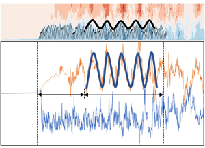
Figure 8(a) shows the streamwise waveform induced by the canopy in the middle row of plants (plant nos 101–200) and the distribution of the instantaneous streamwise velocity ux in case C1. It is evident that, after the flow takes place in the vegetation region over a certain distance and after the turbulence is fully developed, the vegetation canopy induces a waveform with an approximate spatially periodic distribution. Previous studies showed that the periodic waving motion of vegetation is caused by the KH instability at the flow–vegetation interface (Ghisalberti & Nepf Reference Ghisalberti and Nepf2002; Luhar & Nepf Reference Luhar and Nepf2011; Tschisgale et al. Reference Tschisgale, Löhrer, Meller and Fröhlich2021; Wang et al. Reference Wang, He, Dey and Fang2022). The main reason for the formation of the KH vortices is attributed to the velocity difference inside and outside the vegetation canopy. Moreover, the vegetation coherent waving motion caused by the KH vortices also acts on the flow, resulting in an uneven streamwise distribution of flow velocity. The obstruction of the vegetation to the flow is different at the crest and at the trough of the vegetation canopy wave. The waterward area of vegetation at the crest of the waveform is larger, which has a greater obstruction effect to the flow. The instantaneous streamwise flow velocity inside the vegetation decreases or even appears to be negative. On the other hand, the flow velocity above the canopy is higher, while the situation at the trough of the waveform is the reverse. Therefore, the flow velocity distribution also presents a periodic distribution of alternating peak and trough values, both above and below the vegetation canopy (figure 8b).

Figure 8. (a) Waveform induced by the canopy of submerged flexible vegetation and the distributions of the instantaneous streamwise flow velocity ux inside and outside the canopy and (b) streamwise distributions of the instantaneous streamwise flow velocity ux at the vertical distances z/h = 1.5 (above) and 0.5 (below). Note that the top of the vegetation canopy refers to at z/h = 1.0.
Figure 9 presents the vertical distributions of the instantaneous streamwise flow velocity at the peak and the trough of the vegetation waveform and the time-averaged streamwise velocity. In terms of the time-averaged velocity, the influence of the vegetation on the flow is equivalent to the ‘mixing layer’ in figure 9(a) (Ghisalberti & Nepf Reference Ghisalberti and Nepf2002, Reference Ghisalberti and Nepf2004). The mean velocity difference inside and outside the vegetation canopy is approximately 1.6Ub. The average equivalent canopy height of vegetation is approximately  ${\bar{z}_v} = 0.65h$. At the crest of the waveform, the tilt angle of the vegetation is smaller and the equivalent canopy height is higher, at approximately zv = 0.9h (the canopy height is zv = 1.0h when the water is still). Accordingly, due to the larger area of vegetation waterward surface, the obstruction effect on the flow is stronger; therefore, the velocity difference inside and outside the canopy is larger. A negative velocity zone is formed inside the vegetation, and the difference between the velocity inside and outside the canopy is approximately 3Ub. At the trough of the vegetation waveform, the tilt angle of the vegetation is larger; therefore, the equivalent canopy height is lower, at approximately zv = 0.3h. As the area of the waterward surface of vegetation decreases, the obstruction effect of vegetation on the flow weakens. Hence, the velocity difference inside and outside the canopy is smaller than that at the wave crest. The velocity difference inside and outside the canopy is approximately Ub. Different from the average velocity distribution and the velocity distribution at the wave crest, the vertical distribution of the velocity at the trough of the waveform is closer to the logarithmic law of velocity distribution, which is quite different from the hyperbolic–tangent curve of the average velocity ${\bar{u}_x}$.

Figure 9. Streamwise velocity distributions with flexible submerged vegetation after turbulence is fully developed in case 1 (i.e. in the amplitude stable region described in § 4.2). The blue curve represents the vertical distribution of the dimensionless time-averaged streamwise flow velocity  ${\bar{u}_x}/{U_b}$. The grey curve signifies the vertical distribution of the dimensionless instantaneous streamwise velocity ux/Ub at the wave crest of the waveform. The orange curve shows the vertical distribution of the dimensionless instantaneous streamwise velocity ux/Ub at the wave trough of the waveform. The blue, grey and orange dotted lines represent the equivalent canopy height under the three circumstances. The ‘mixing layer’ marked in the figure is divided according to the hyperbolic tangent portion of the ${\bar{u}_x}$ distribution (Ghisalberti & Nepf Reference Ghisalberti and Nepf2002).
4.1.3. Turbulence structure formed by flow–vegetation interaction
Vorticity ω, as the curl of the flow velocity vector, is usually used to characterise the vortex structure in the flow. However, its magnitude is affected by the shear stress, that is, the zone with large shear stress has large vorticity even if there is no swirl motion. Therefore, it is not suitable to analyse the turbulent flow structure in the presence of vegetation due to the existence of the strong shear stress layer at the flow–vegetation interface. Therefore, the Q criterion (da Silva & Pereira Reference da Silva and Pereira2008), which eliminates the influence of shear stress, can be effectively used to demonstrate the vortex structure in the vegetation region.
The Q criterion can be estimated from the following expression:
 \begin{equation}Q ={-} \frac{1}{2}\left[ {{{\left( {\frac{{\partial {u_x}}}{{\partial x}}} \right)}^2} + {{\left( {\frac{{\partial {u_y}}}{{\partial y}}} \right)}^2} + {{\left( {\frac{{\partial {u_z}}}{{\partial z}}} \right)}^2}} \right] - \frac{{\partial {u_x}}}{{\partial y}}\frac{{\partial {u_y}}}{{\partial x}} - \frac{{\partial {u_x}}}{{\partial z}}\frac{{\partial {u_z}}}{{\partial x}} - \frac{{\partial {u_y}}}{{\partial z}}\frac{{\partial {u_z}}}{{\partial y}}.\end{equation}
For Q > 0, the vortices prevail in the flow zone.
Figure 10 shows the distribution of the isosurface of Q = 0, where the low intensity eddies formed by random flow turbulence are filtered. According to the isosurface of Q, the vortex position in the flow can be determined. It can be seen that the vortex structure in the flow primarily presents a wavy ribbon distribution along the flow–vegetation interface. Therefore, the vortices (or the eddies) in a flow with submerged vegetation mainly exist near the interfacial zone. This is quite consistent with the findings of previous studies (O'Connor & Revell Reference O'Connor and Revell2019; Tschisgale et al. Reference Tschisgale, Löhrer, Meller and Fröhlich2021; Wang et al. Reference Wang, He, Dey and Fang2022). Due to the vegetation coherent waving motion, the flexible vegetation canopy exhibits a waveform distribution. Thus, the distributions of the vortex structure differ at different locations. At the crest of the waveform induced by the vegetation canopy, the vortices (or the eddies) are distributed at a larger height as the equivalent canopy height of vegetation rises, and they even prevail near the free surface. In contrast, at the trough of the waveform, the eddies invade down close to the bed. Although there is no significant difference in the width of the vortex ribbon at the crest and the trough of the waveform induced by vegetation canopy, it is apparent that the distribution of the isosurface of Q is denser at the crest than at the trough. Accordingly, the intensity of the vortex at the crest is obviously higher than that at the trough. This corresponds with the trend indicated by the difference in velocity distributions at different locations in § 4.1.1.

Figure 10. Distribution of isosurface of Q = 0 near the vegetation canopy for 45 < x/h < 60. The two yellow curves identify the streamwise ribbon distribution of the isosurface of Q. The green curves represent the vegetation.
Figure 11 shows the fields of the velocity fluctuation and the isoline of pressure fluctuation. According to the fluctuation values of these two quantities, the direction, intensity and the scale of the eddies in the flow can be obtained. It is apparent that, at the crest and the trough of a waveform induced by the vegetation, the streamlines of velocity fluctuation show two vortices with opposite sense rotations. At the crest, the flow velocity above the vegetation canopy is greater than the average flow velocity, while the flow velocity below the canopy is lower than the average flow velocity (see § 4.1.1), forming a clockwise vortical motion. The directions of velocity fluctuation and vortical motion are opposite at the trough. According to the isoline of pressure fluctuation, it can be observed that the intrusion degree of the vortex at the trough is significantly greater than that at the crest, being consistent with the result obtained from the Q criterion.

Figure 11. Distributions of velocity fluctuation u′ in two wavelength ranges of the waveform induced by the vegetation coherent waving motion in case 1 with (a)  $53 < x/h < 58$ and (b) $38 < x/h < 43$. The black solid curves represent the isolines of the pressure fluctuation p′, which is used to mark the spatial scale of the KH vortex. The yellow circles represent the streamlines of u′.
The streamwise scale of the two vortices determines the wavelength of the waveform induced by the vegetation coherent waving motion. The vertical scale and the depth of invasion of the two vortices into the vegetation determine the amplitude of the coherent waving motion. The streamwise spread speed of the vortices determines the frequency of the plant waving motion. These characteristics are influenced by the various factors, such as flow conditions and vegetation distribution, and are discussed in §§ 4.2–4.4.
4.2. Coherent waving motion of submerged flexible vegetation
4.2.1. Basic characteristics of flexible vegetation swaying
In order to explore the coherent waving motion of the submerged flexible vegetation, it is necessary to verify the periodic movement of a single plant over time for a given flow condition, and to find out its amplitude variational characteristics. Figure 12 shows the maximum changes in canopy height based on the stationary canopy height Δzv/h (that is, the height difference between the highest point and the lowest point of the canopy height of a plant, which shows the swaying amplitude of an individual plant) in the middle row (in the spanwise direction) of the plants (plant nos 101–200) in the streamwise direction during a period of 65 s captured in case C1.

Figure 12. (a) Average (curve), maximum (upper edges of the vertical lines) and minimum (lower edges of the vertical lines) values of the canopy height zv/h and (b) streamwise distribution of the tilt angle θ in the middle row of plants (plant nos 101–200) in a period of 65 s after the fully developed turbulent flow in the C1 case. The length of the vertical line represents (a) the maximum changes in canopy height Δzv/h and (b) tilt angle Δθmax of vegetation during 65 s. The green region is the vegetation frontal region, the blue region the amplitude increasing region and the yellow region the amplitude stable region.
According to the maximum change of vegetation canopy height Δzv (whose value is equal to the reduction in canopy height), submerged vegetation can be divided into three regions along the streamwise direction, namely, the vegetation frontal region, the amplitude increasing region and the amplitude stable region (shown in figures 12 and 13). As the flow velocity drops rapidly after entering the vegetation region (figures 13 and 7), among the three regions, the plants in the vegetation frontal region are most affected by the flow impulse, that is, the average force in the streamwise direction on the plants is the largest. Therefore, in this region, the average tilt angle  $\bar{\theta }$ of vegetation is the largest among all three regions, and the average canopy height ${\bar{z}_v}$ decreases the most. In case C1, the average canopy height of plant no. 101 at the forefront of the vegetation is ${\bar{z}_v} = 0.4h$, while the average tilt angle is $\bar{\theta } = 1.30$ (figure 12). Before the flow enters the vegetation region, the turbulence in the flow is dominated by its own random velocity fluctuations, and the turbulence intensity is much lower as compared with that in the vegetation region, since its vertical velocity gradient is much lower (figure 13b). Therefore, in the three regions, the maximum change of the plant tilt angle Δθmax in the vegetation frontal region is the smallest, and the maximum change of canopy height Δzv is also the smallest. In case C1, the vegetation frontal region contains seven plants in each row (including plant nos 101–107 as an example, corresponding to the range of 15 < x/h < 18 in figure 7). In the vegetation frontal region, the average canopy height ${\bar{z}_v}$, the maximum change of canopy height Δzv and the maximum change of plant tilt angle Δθmax increase rapidly, while the plant average tilt angle $\bar{\theta }$ decreases rapidly. In the amplitude increasing region, the spatial streamwise gradient of the flow velocity is significantly lower than that in the vegetation frontal region (figures 13b and 7). In this region, the streamwise variation of the average tilt angle $\bar{\theta }$ slows down, while that of the average canopy height ${\bar{z}_v}$ reaches a relatively stable state. In case C1, the average tilt angle and the average canopy height of the plants gradually decreases and increases, respectively, in the amplitude increasing region and finally, they stabilise at around $\bar{\theta } = 0.86$ and ${\bar{z}_v} = 0.65h$. The turbulence at top of the canopy in the amplitude increasing region is dominated by the KH instability owing to the flow velocity gradient (figure 7). It is different from that in the vegetation frontal region, due to an increase in velocity difference above and below the vegetation canopy (figure 13). The turbulence intensity is much greater than the random flow turbulence, and therefore the amplitude of the plant fluctuation in the amplitude increasing region is much greater than that in the vegetation frontal region. Therefore, although the temporal average values of the tilt angle $\bar{\theta }$ and canopy height ${\bar{z}_v}$ of the plants tend to be stable in the streamwise direction in the amplitude increasing region, their amplitudes of changes, Δθmax and Δzv, continue to increase. In case C1, the amplitude increasing region contains 26 plants in each row (including plant nos 108–133 as an example, corresponding to the range of 18 < x/h < 33 in figure 7, where $\bar{u}$ at canopy height keeps basically stable, while τxz increases significantly along the streamwise direction). The average flow velocity above and below the vegetation canopy is basically stable in the streamwise direction after the flow enters the amplitude stable region. Therefore, the average forces on the plants in this region do not vary with the change of spatial position of the plants. The average canopy height ${\bar{z}_v}$ and the average tilt angle $\bar{\theta }$ of different plants in the amplitude stable region are essentially the same and fluctuate in a small range. In case C1, the average canopy height of vegetation in the streamwise direction is stable at around ${\bar{z}_v} = 0.65h$ in the amplitude stable region, while the average tilt angle is stable at around $\bar{\theta } = 0.86$. In addition, the intensity of the KH vortices near the canopy in the amplitude stable region does not vary with the spatial position, because the shear stress at the canopy height does not vary with the spatial position in the streamwise direction (figure 7). As a result, the range of the plant motion at different locations in this region is almost same. Both the maximum changes of canopy height Δzv and the tilt angle Δθmax are stable at their respective fixed values. In case C1, the maximum change of canopy height of 67 plants (plant nos 134–200, corresponding to the range of 33 < x/h < 64.5 in figure 7, where the change of shear stress τxz in the streamwise direction is not significant) in the middle row in the amplitude stable region is stable at around Δzv = 7.44D in the streamwise direction, while the maximum tilt angle is stable at around Δθmax = 1.00. It can be predicted that the range of the plants contained in the three regions is different for the conditions of different flow velocities, different vegetation densities and different submergences. Specific differences are analysed in §§ 4.3–4.5.

Figure 13. (a) Distribution of the time-averaged streamwise flow velocity  ${\bar{u}_x}$ in the y/h = 0 plane and (b) streamwise distribution of the dimensionless time-averaged streamwise flow velocity ${\bar{u}_x}/{U_b}$ above (z/h = 1.5, orange line), at (z/h = 1.0, blue line) and below (z/h = 0.5, green line) the stationary canopy of submerged vegetation.
In order to verify the coherent waving motion of flexible submerged vegetation, it is required to start with two points. The first point is to verify that individual plants in the vegetation swing periodically with time and this period does not vary with spatial position. The second point is to verify the periodic distribution of the canopy height of the vegetation, as a whole, in the spatial location. Taking case C1 to verify the vegetation coherent waving motion, the time period of individual plant movement and the spatial period of the whole vegetation fluctuation are calculated. The movement states of plants in the vegetation frontal region and the amplitude increasing region are unstable, since their average canopy height and swing amplitude vary considerably in space. Therefore, the plants in these two regions are not suitable for analysing the time period of individual plants. In addition, the spatial period of vegetation coherent waving motion is unstable in these two regions due to the insufficiently developed turbulence in the flow. Therefore, in this part, the characteristics of the plant movement period in the amplitude stable region are mainly considered.
4.2.2. Time periodicity of coherent waving motion
Figure 14(a) plots the time series dataset of canopy height zv of an individual plant (plant no. 177) in the amplitude stable region in case C1. The moving average method and Butterworth filter are used to filter the time series dataset of the plant canopy top to eliminate the impact of random flow turbulence on vegetation movement and to highlight the KH instability role in the vegetation coherent waving motion. The time series dataset of the amplitude of the vegetation coherent waving motion  $\mathrm{\Delta }{\hat{z}_v}/h$ dominated by the KH instability is plotted in figure 14(b). The random amplitude of plant fluctuation $\mathrm{\Delta }{z^{\prime}_v}/h$ (where $\mathrm{\Delta }{z^{\prime}_v} = \mathrm{\Delta }{z_v}\unicode{x2013}\mathrm{\Delta }{\hat{z}_v}$ and $\mathrm{\Delta }{z_v} = {z_v}\unicode{x2013}{\bar{z}_v}$) dominated by the random flow turbulence is eliminated through use of the filter. It can be found that $\mathrm{\Delta }{\hat{z}_v}/h$, which is dominated by the KH instability, shows alternating changes of positive and negative magnitudes over time, where the periodic change is relatively stable. In contrast, $\mathrm{\Delta }{\hat{z}_v}/h$, which is dominated by random flow turbulence, shows irregular positive and negative high frequency variations. In addition, the variation of $\mathrm{\Delta }{\hat{z}_v}$ is significantly larger than that of $\mathrm{\Delta }{z^{\prime}_v}$. Figure 14(b) shows that the main distribution range of $\mathrm{\Delta }{\hat{z}_v}$ is ${-}0.2 < \mathrm{\Delta }{\hat{z}_v}/h < 0.2$, while $\mathrm{\Delta }{z^{\prime}_v}$ is mainly distributed in the range of ${-}0.1 < \mathrm{\Delta }{z^{\prime}_v}/h < 0.1$. This can also indirectly indicate that the strength of the vortex caused by the KH instability is significantly greater than that produced by the random flow turbulence.

Figure 14. (a) Time series dataset of the canopy height zv/h of the vegetation in the amplitude stable region (taking plant no. 177 as an example) in the C1 case and (b) time series dataset of the smoothed canopy height change  $\mathrm{\Delta }{\hat{z}_v}/h$ obtained by the moving-average method and Butterworth filter, eliminating the noise $\mathrm{\Delta }{z^{\prime}_v}/h$ with the filter.
The amplitude–frequency characteristic relation of the canopy height change caused by the vegetation coherent waving motion can obtained by the FFT of  $\mathrm{\Delta }{\hat{z}_v}/h$ (figure 15a). However, the same data processing method is used to obtain the amplitude–frequency characteristic curve of the instantaneous streamwise flow velocity ux above the average canopy height of plant no. 177 (figure 15b). In addition, the frequency spectra of canopy height zv and streamwise flow velocity ux are plotted separately to analyse the relationship between the change of flow velocity and the frequency of vegetation coherent waving motions (figures 15c and 13d) (Monin & Yaglom Reference Monin and Yaglom2007; Dey et al. Reference Dey, Das, Gaudio and Bose2012; Wang et al. Reference Wang, He, Dey and Fang2022). The energy spectrum function E( f) or E(kw) can be regarded as the kinetic energy of plant motion kp or the TKE k′ energy density of periodic plant movement or velocity fluctuation (eddies) with frequency f or wave number kw, which satisfies
 \begin{equation}k = \int_0^\infty {E(\lambda )\,\textrm{d}\lambda } ,\end{equation}
where k is the kinetic energy of vegetation kp and the TKE k′ when analysing the coherent waving motion of vegetation and the fluctuation of flow velocity, respectively; λ is the frequency f and wavenumber kw, when analysing time periodicity and space periodicity, respectively.

Figure 15. Amplitude–frequency characteristic curves of the time series dataset of (a) the canopy height change  $\mathrm{\Delta }{\hat{z}_v}/h$ and (b) the streamwise flow velocity ux above the top of the canopy obtained by the FFT. Frequency spectra of (c) the canopy height change $\mathrm{\Delta }{\hat{z}_v}/h$ and (d) the streamwise flow velocity ux. Here, ${\hat{A}_{zv}}$ and ${\hat{A}_{ux}}$ are the amplitude corresponding to the main peak of plant periodic movement and velocity periodic fluctuation, respectively.
It is evident from figure 15(a) that there is a peak with frequency f = 0.30 Hz and amplitude  ${\hat{A}_{zv}} = 0.20h$ in the amplitude–frequency characteristic curve of vegetation canopy height change. Also, the frequency spectrum (figure 15c) exhibits that the spectral intensity of vegetation movement is maximum at the frequency of f = 0.29 Hz. It can be inferred that, in case C1, the plants in the amplitude stable region move in a periodic fluctuation with a large amplitude at the main frequency of fm = 0.30 Hz. A close examination of the amplitude–frequency spectrum of the streamwise flow velocity ux (figure 15b) reveals that there is a peak point with frequency f = 0.31 Hz in the flow velocity fluctuation. Besides, a point with the maximum spectral intensity with frequency f = 0.30 Hz can also be observed in the frequency spectrum (figure 15d). The hyperbolic tangent curve, ${\bar{u}_x}\; - {U_b} = {U_b}\textrm{tanh[(}z - {z_{{U_b}}}\textrm{)/(2}\delta \textrm{)]}$, where ${z_{{U_b}}}$ is the height, ${\bar{u}_x} = {U_b}$ and δ is the fitting parameter, is used to fit the vertical distribution of the average streamwise flow velocity in the mixing layer (Ghisalberti & Nepf Reference Ghisalberti and Nepf2002) in figure 9. Furthermore, the Strouhal number St = fδ/Ub (Ho & Huerre Reference Ho and Huerre1984) was calculated from the obtained parameter δ and the frequency f calculated by FFT and the frequency spectrum in figure 15. The calculation result shows St = 0.033, which is consistent with St = 0.032 in Ho & Huerre (Reference Ho and Huerre1984).
The above mechanism indicates that the frequency of vegetation coherent waving motion is the same as that of flow velocity fluctuation (KH vortices). Previous studies have also shown that the frequency of monami is basically consistent with the frequency of the downstream flow velocity (Ghisalberti & Nepf Reference Ghisalberti and Nepf2002). The coherent waving motion of vegetation is mainly affected by the KH vortices, and the formation of the KH vortices is also highly correlated with the existence and movement of the vegetation.
Analysing the amplitude and frequency characteristics of vegetation movement and flow velocity fluctuation obtained by amplitude–frequency curves and frequency spectrum curves in figure 15, the coherent waving motion of vegetation and periodic fluctuation of flow velocity are fitted and plotted in figure 16. It is apparent that the time periodicity of vegetation coherent waving motion and velocity fluctuation obtained by the FFT method are in good agreement with the actual movement of vegetation and the change of instantaneous velocity with time. The canopy height of vegetation zv and the streamwise flow velocity ux show a significant temporal periodic trend. The difference between the actual variation and the fitted periodic variation curve of canopy height (between Δzv and  $\mathrm{\Delta }{\hat{z}_v}$) and flow velocity (between ux and ${\hat{u}_x}$) is caused by the random turbulence in the flow. In addition, comparing the time periods of vegetation coherent waving motion and velocity fluctuation, it is revealed that the change of the period of flow velocity ux above the top of the canopy (at z/h = 1.0) is consistent with that of vegetation canopy height, and there is no phase difference, that is, the positions of wave peaks and troughs are the same. This indicates that, at the crest of the vegetation canopy, the velocity above the top of the canopy is also at the crest, while at the trough of the vegetation canopy, the velocity is also exactly at the trough. This is consistent with the trend shown in figure 9. This indicates that the flow velocity and vegetation coherent waving motion are mutually affected and significantly correlated.

Figure 16. Comparisons of the original value (blue curve) with the periodic value (orange curve) obtained by the FFT of (a) the changes of canopy height Δzv/h (blue) and  $\mathrm{\Delta }{\hat{z}_v}/h$ (orange) and (b) the instantaneous streamwise flow velocity ux/Ub (blue) and ${\hat{u}_x}/{U_b}$ (orange) in case C1 (taking plant no. 177 as an example).
4.2.3. Spatial periodicity of coherent waving motion
In the amplitude stable region, we can prove that the vegetation moves in periodic coherent waving motion as a whole by showing that the canopy height of each row of the plants in this region is periodically distributed in spatial position. Figure 17 plots the canopy height distribution of the plants in the middle row along the spanwise direction in the amplitude stable region (plant nos 134–200, containing a total 67 plants) in case C1 at a certain time. It can be seen that, in the streamwise direction, the canopy height of plants in the amplitude stable region is evenly distributed around the equilibrium position  ${\bar{z}_v}$, showing a trend of evenly alternating up and down around the equilibrium position in spatial position. The mean and standard deviation of the canopy height of 67 plants are ${\bar{z}_v} = 0.66h$ and σzv = 0.14h, respectively. It can be inferred that the 67 plants show a spatial fluctuation distribution with the mean value of ${\bar{z}_v} = 0.66h$ and the amplitude of Azv = σzv = 0.14h.

Figure 17. Distribution of the dimensionless canopy height zv/h in the middle row of plants in the amplitude stable region (plant nos 134–200, containing a total 67 plants, covering a range with 31.5 < x/h < 64.5) in the streamwise direction at a random moment in case C1.
By using the FFT method, the discrete spatial sequence dataset of the canopy height zv of 67 plants and the instantaneous streamwise flow velocity ux above the top of the canopy (at z/h = 1.0) are expanded in series. Then, the amplitude–frequency relationship of the spatial fluctuation distribution of canopy height zv and flow velocity ux is obtained, as shown in figure 18(a,b). In addition, the wavenumber spectra are also drawn (figure 18c,d) to determine the waveform of the vegetation coherent waving motion and the spatial scale of the KH vortices in the mixing layer near the canopy. This helps to analyse the relationship between the wavelength of the vegetation coherent waving motion and the scale of the KH vortices. It is evident that, akin to the time series dataset of individual plant canopy height, the amplitude–frequency curve of the spatial distribution of canopy height of a row of plants in the amplitude stable region also contains a peak point that indicates the main periodic movement characteristic of the vegetation canopy (figure 18a). The spatial frequency, commonly known as wavenumber, and amplitude of the main peak at the peak point are kw = 0.21/h and  ${\hat{A}_{zv}} = 0.20h$, respectively. Accordingly, the fluctuation distribution period (wavelength) of plant canopy is Lw = 1/kw = 4.8h. According to the results of the FFT, the plant canopy height presents a spatially periodic distribution with the wavelength Lw = 4.8h and the amplitude of the main peak ${\hat{A}_{zv}} = 0.20h$. This is consistent with the amplitude of the time-periodic movement of individual plant calculated in § 4.2.2. It also corroborates the reliability of using the FFT to analyse the characteristics of the vegetation coherent waving motion. Due to the random flow turbulence, the canopy height fluctuates randomly with the amplitude ${A^{\prime}_{zv}} = |{A_{zv}} - {\hat{A}_{zv}}|= 0.06h$ on the basis of the periodic distribution. In the wavenumber spectrum curve (figure 18c), a peak point with the highest spectral intensity at kw = 0.22/h can be observed, which also confirms the results of the amplitude–frequency characteristic curve. Similarly, the FFT method is used to analyse the velocity above the canopy (at z/h = 1.0). The velocity also shows a significant tendency of periodic distribution in space. In the amplitude–frequency characteristic curve, there is a peak with wavenumber kw = 0.19/h and amplitude ${\hat{A}_{zv}} = 0.65{U_b}$. At the same time, the peak point with highest spectral intensity with wavenumber of kw = 0.19/h is also observed in the wavenumber spectra. The above phenomenon indicates that the canopy height of vegetation zv and the velocity distribution above the top of the canopy ux have significant periodic distribution trends in space, and their wavenumbers are basically the same. This specifies that, in space, the coherent waving motion of vegetation and streamwise velocity fluctuation (streamwise scale of the KH vortices) in the mixing layer are of the same frequency, and there is a significant correlation between them.

Figure 18. Amplitude–frequency characteristic curves of the spatial sequence dataset of (a) the canopy height zv/h in the middle row of plants and (b) instantaneous streamwise flow velocity ux above the top of the canopy (at z/h = 1.0) in the amplitude stable region (plant nos 134–200) in the streamwise direction in case C1. The wavenumber spectra of (c) the canopy height zv/h and (d) the flow velocity ux.
Figure 19 shows the actual canopy heights zv of plant nos 165–200 at a random moment (green elements) and the waveform created by the canopy heights  ${\bar{z}_v}$ obtained by the FFT method (red curve). The fitting curve of ${\bar{z}_v}$ corresponds with the actual canopy heights zv. Therefore, the wavelength Lw and amplitude ${\hat{A}_{zv}}$ (half of the wave height) of the vegetation coherent waving motion obtained by the FFT method is accurate and reliable.

Figure 19. Actual positions of plant nos 165–200 at a random moment (green elements) and the waveform obtained by the FFT method (red curve). The red curve identifies the wavelength Lw and amplitude  ${\hat{A}_{zv}}$ of the waveform of the vegetation coherent waving motion obtained by the FFT method.
4.3. Effect of flow velocity on the coherent waving motion
Previous studies showed that an increase in Reynolds number can significantly change the offset angle and swing amplitude of submerged flexible vegetation (Luhar & Nepf Reference Luhar and Nepf2011; Wang et al. Reference Wang, He, Dey and Fang2022). In addition, due to an increase in Reynolds number and averaged streamwise velocity, the intensity of the KH vortices around the flow–vegetation interface and their propagation velocity in the downstream increase. Therefore, it can be concluded that the Reynolds number significantly affects the period (both temporal and spatial) and the amplitude of vegetation coherent waving motion.
In §§ 4.1 and 4.2, the frequency, amplitude and wavelength of vegetation coherent waving motion are found to have correlation with the frequency and spatial scale of the KH vortices and the formation of the KH vortex is found to be closely related to the turbulence intensity in the mixing layer near the canopy height (Ghisalberti & Nepf Reference Ghisalberti and Nepf2002; Wang et al. Reference Wang, He, Dey and Fang2022). Figure 20 shows the vertical and streamwise distributions of the TKE for different Reynolds numbers. It is observed that, for different Reynolds numbers, the TKE is mainly distributed in the mixing layer near the average canopy height, and the magnitude of the TKE is the maximum at the canopy height  ${\bar{z}_v}$. Examining the distributions of the TKE for different flow velocities, it can be seen that the magnitude of the TKE in the mixing layer increases significantly with an increase in Reynolds number. The amplification of turbulence intensity in the mixed layer indicates the intensification of the velocity fluctuation frequency. Therefore, it can be predicted that the frequency f of vegetation coherent waving motion increases with an increase in flow velocity. As the flow velocity increases, the average swaying angle of vegetation $\bar{\theta }$ increases and the average canopy height ${\bar{z}_v}$ decreases. However, from the vertical distributions of the TKE in figure 20(a–d), it can be seen that, with an increase in flow velocity, the vertical distribution range of the TKE increases significantly, implying that the coverage of the mixing layer increases significantly. Therefore, the vertical scale of the KH vortex also increases with an increase in flow velocity. It can be predicted that the amplitude of vegetation coherent waving motion ${\hat{A}_{zv}}$ also increases with an increase in flow velocity.

Figure 20. Distributions of the TKE in (a) case 1, (b) case 2, (c) case 3 and (d) case 4 in the xz plane with y/h = 0, where the centre line of plant nos 101–200 is located at a streamwise distance of dx = 10h. The flow velocity gradually decreases from (a) to (d).
Figure 21 shows the position and spatial scale of two vortices with opposite rotational directions at the crest and the trough of the waveform induced by the vegetation coherent waving motion according to the fields of the velocity fluctuation. It is found that, as the flow velocity (that is, the Reynolds number Re) increases, the streamwise special scale of the vortices at the flow–vegetation interface decreases, while the vertical scale increases. An increase in flow velocity leads to an increase in the plant tilt angle, which leads to a decrease in the distribution heights of the vortices. It can be concluded that, with an increase in flow velocity, the wavelength Lw of the waveform induced by the vegetation coherent waving motion decreases, while the amplitude  ${\hat{A}_{zv}}$ increases. As the flow velocity increases, it leads to an increase in rotational speed of vortices in the streamwise direction uv. The frequency of vegetation coherent waving motion satisfies f = 1/T = uv/Lw. Therefore, the frequency of the vegetation coherent waving motion increases with an increase in flow velocity.

Figure 21. Projected fields of velocity fluctuation u′ on the y/h = 0.0 plane for different Reynolds numbers over a streamwise distance of dx = 10h. The black arrows indicate the vectors of the velocity fluctuation u′. The yellow curves and arrows indicate the position and rotational direction of the vortices at the flow–vegetation interface. (a)–(d) four groups of experiments, cases C1–C4, respectively, corresponding to Reynolds numbers Re = 50 000 − 20 000.
In order to verify the prediction of the characteristics of vegetation coherent waving motion based on the aforementioned physical mechanism, the frequency and wavenumber spectra of vegetation coherent waving motion for different flow velocities are plotted in figure 22. In addition, the frequency, amplitude and wavelength of vegetation coherent waving motion in cases C1–C7 are quantitatively listed in table 2. It can be seen that the frequency corresponding to the peak point gradually increases with an increase in flow velocity, and the spectral intensity gradually increases, which suggests that an increase in Reynolds number causes an increase in the frequency f and a decrease in the amplitude  ${\hat{A}_{zv}}$ of the vegetation coherent waving motion, being consistent with the experimental results of Ghisalberti & Nepf (Reference Ghisalberti and Nepf2002). Besides, the data in table 2 confirm this relationship. The change of plant specific gravity ρIBM/ρw has little effect on the frequency corresponding to the peak point of frequency spectrum, but it increases the spectral intensity at the peak. This implies that the frequency f of vegetation coherent waving motion is independent of the specific gravity ρIBM/ρw of the plant itself, but the amplitude ${\hat{A}_{zv}}$ of coherent waving motion of plants with higher density is larger. The wavenumber spectra in figure 22(e–h) quantitatively show the variational trend of the spatial periodicity characteristics of vegetation coherent waving motion with the flow velocity. It is evident that, with an increase in flow velocity, the wavenumber kw corresponding to the peak point of the wavenumber spectrum increases significantly, implying that the wavelength Lw of vegetation coherent waving motion decreases. It is observed that the wavenumber kw corresponding to the peak point does not vary with the plant specific gravity ρIBM/ρw, implying that the wavelength Lw of coherent waving motion of the vegetation is also independent of plant specific gravity ρIBM/ρw.

Figure 22. (a)–(d) Frequency spectra and (e)–(h) wavenumber spectra of vegetation coherent waving motion for different Reynolds numbers. The solid black lines represent the vegetation with specific gravity ρIBM/ρw = 0.3, while the dashed blue lines represent the vegetation with specific gravity ρIBM/ρw = 0.5. Panels (a)–(d) and (e)–(h) represent the changes of Reynolds number Re = 50 000 − 20 000.
Table 2. Results of the frequency, amplitude and wavelength of cases C1–C7.

In conclusion, the flow velocity has a significant influence on the frequency and amplitude of vegetation coherent waving motion. From the perspective of the temporal periodicity of coherent waving motion, the larger Reynolds number corresponds to the higher time frequency f, the shorter time period T and the larger amplitude  ${\hat{A}_{zv}}$ of vegetation periodic coherent waving movement. In terms of spatial periodicity, the larger Reynolds number corresponds to the higher wavenumber kw, the shorter wavelength Lw and the larger amplitude ${\hat{A}_{zv}}$ of the waveform induced by the vegetation canopy. From the visual perspective, the larger Reynolds number is associated with the waveform with the shorter wavelength, larger amplitude and faster spread speed in the streamwise direction.
4.4. Effect of vegetation distribution density on coherent waving motion
The distribution density of submerged vegetation significantly affects the velocity distribution of vegetated flow. In addition, the vegetation distribution density also affects the intensity and the scale of the KH vortices at the flow–vegetation interface (Nepf Reference Nepf2012). Therefore, the vegetation distribution density influences the frequency and the amplitude of coherent waving motion of submerged flexible vegetation.
Figure 23 shows the vertical and streamwise distributions of the TKE for different vegetation distribution densities. It is apparent that, as the density of vegetation distribution becomes larger, both the magnitude and distribution range of the TKE near the vegetation canopy increase significantly. For cases C1 (Dv/h = 0.5) and C8 (Dv/h = 1.0), the TKE has a tendency to have a uniform distribution along the streamwise direction in the mixing layer. This trend signifies that the swaying of the vegetation canopy is primarily affected by the KH instability within the mixing layer. However, in case C9 (Dv/h = 2.0), the TKE is mainly distributed downstream of an individual plant and decays rapidly before the flow reaches the next plant. This indicates that, when the plants are distributed sparsely, the flow cannot form a mixing layer near the vegetation canopy, and vegetation swaying is mainly affected by the flow impulse and random turbulence.

Figure 23. Distributions of the TKE in (a) case 1, (b) case 8 and (c) case 9 in the xz plane with y/h = 0, where the centre line of plant nos 101–200 is located at a streamwise distance of dx = 10h. The plant spacing Dv/h gradually increases from (a) to (c).
Since the turbulence intensity in flow and the vertical scale of mixing layer increase with an increase in vegetation distribution density, it can be predicted that the frequency and the amplitude of vegetation coherent waving motion increase with an increase in vegetation distribution density.
Figure 24 shows the fields of the velocity fluctuation and the distribution of vortices at the flow–vegetation interface for different vegetation distribution densities. It can be observed that, as the plant spacing Dv increases (that is, a decrease in vegetation distribution density), both the streamwise and vertical scales of the vortices at the flow–vegetation interface increase and the tendency of the vortex intrusion into the vegetation region also increases. It can be predicted that, with an increase in plant spacing, both the wavelength Lw and amplitude  ${\hat{A}_{zv}}$ of the waveform induced by vegetation coherent waving motion increase. Due to a significant increase in wavelength Lw and a constant averaged streamwise flow velocity ${\bar{u}_x}$, the streamwise spreading speed of the vortices uv is basically not affected; hence, the frequency of vegetation coherent waving motion fm = uv/Lw also significantly increases.

Figure 24. Projected fields of velocity fluctuation u′ in the y/h = 0.0 plane in (a) case C1, (b) case C8 and (c) case C9 for different vegetation distribution densities within a streamwise reach of dx = 10h. The arrows represent the vectors of the velocity fluctuation u′. The yellow curves and arrows indicate the position and the rotational direction of the vortices at the flow–vegetation interface. Since the wavelength Lw of the waveform induced by the vegetation coherent fluctuations in case C8 exceeds 10h (Lw = 22.35h, as calculated by the FFT method below), only the half-wavelength is plotted in (c).
Figure 25 shows the frequency and wavenumber spectra of vegetation coherent waving motion for different vegetation distribution densities. In addition, table 3 lists the frequency f, amplitude  ${\hat{A}_{zv}}$ and wavelength Lw of vegetation coherent waving motion in cases C1, C8 and C9. In figure 25, as the plant spacing Dv increases, the peak points of the frequency and wavenumber spectra have a tendency to shift to the left, implying that the frequency f and wavenumber kw decrease, and correspondingly, the time period T and wavelength Lw of coherent waving motion increase. With an increase in plant spacing Dv, the spectral intensity corresponding to the peak point of frequency spectrum gradually decreases, suggesting that the amplitude of coherent fluctuations of vegetation gradually decreases. The specific values of frequency f, amplitude ${\hat{A}_{zv}}$ and wavelength Lw in table 3 also show this trend.

Figure 25. (a)–(c) Frequency spectra and (d)–( f) wavenumber spectra of vegetation coherent waving motion for different vegetation distribution densities. Panels (a)–(c) and (d)–( f) represent the different plant spacings Dv/h = 0.5, 1.0 and 2.0.
Table 3. Results of frequency, amplitude and wavelength of cases 1, 8 and 9.

In conclusion, the vegetation distribution density has a significant influence on the characteristics of vegetation coherent waving motion. A denser vegetation distribution results in a higher frequency f and a larger amplitude  ${\hat{A}_{zv}}$ of vegetation coherent waving motion, intensifying the individual plants swing. Spatially, the wavelength Lw of the waveform increases with an increase in plant spacing Dv. This suggests that the waveform becomes gentler as the vegetation distribution becomes sparser.
4.5. Effect of vegetation submergence on coherent waving motion
Compared with the variations of the flow velocity and the vegetation distribution density, the impact of vegetation submergence on flow is more complex. On the one hand, when the relative submergence of vegetation decreases due to a decrease in total flow depth, the relative water-blocking area of vegetation increases, which can cause the flow turbulence to intensify. On the other hand, a decrease in flow depth overlying the vegetation also reduces the spatial scale of the mixing layer. These two factors have opposite effects on the frequency and amplitude of vegetation coherent waving motion, making it difficult to predict their effects on the vegetation coherent waving motion qualitatively.
Figure 26 shows the vertical distribution of the double-average streamwise flow velocity for three specific relative submergences. With an increase in relative submergence, the average flow velocity above and below the vegetation canopy decreases, but the difference in flow velocity does not change much. In addition, the velocity gradient in the mixing layer decreases slightly with an increase in relative submergence.

Figure 26. Vertical distribution of the double-average (time averaged and spatially averaged in the spanwise direction) streamwise flow velocity  ${\bar{u}_x}$ for three relative submergences. The red solid line represents the relative submergence H/h = 3.0, the blue solid line H/h = 2.0 and the black solid line H/h = 1.5. The dotted lines represent velocity gradients in the mixing layer.
From the distribution of the TKE for different relative submergences (figure 27), it can be seen that, with an increase in relative submergence, the peak value of the TKE decreases, but its distribution range expands significantly. This is consistent with the analysis at the beginning of this section.

Figure 27. Distributions of the TKE in (a) case 1, (b) case 10 and (c) case 11 in the xz plane with y/h = 0, where the centre line of plant nos 101–200 is located at a streamwise distance of dx = 10h. The relative submergence H/h gradually increases from (a) to (c).
Figure 28 shows the frequency and wavenumber spectra of vegetation coherent waving motion for different relative submergences, and table 4 lists the specific values of frequency, amplitude and wavelength of vegetation coherent waving motion in cases 1, 10 and 11. Figure 28 reveals that, with an increase in relative submergence, the positions of the peak points of the frequency and wavenumber spectra do not change significantly. Besides, there is no significant difference in the spectral intensity corresponding to the peak points. According to the values in table 4, the variation of the relative submergence has no obvious influence on the frequency f, amplitude  ${\hat{A}_{zv}}$ and wavelength Lw of vegetation coherent waving motion.

Figure 28. (a)–(c) Frequency spectra and (d)–( f) wavenumber spectra of vegetation coherent waving motion for different relative submergences. Panels (a)–(c) and (d)–( f) represent the different relative submergences H/h = 1.5, 2.0 and 3.0.
Table 4. Results of frequency, amplitude and wavelength of cases 1, 10, 11.

To sum up, for the shallow submerged vegetation considered in this study, the variation of submersion depth has no significant impact on the coherent waving motion characteristics of vegetation.
5. Conclusions
In this study, a three-dimensional numerical model of the interaction between the flow and the highly flexible submerged vegetation is developed applying LES and the IBM to study the characteristics of the coherent waving motion of vegetation. Compared with the previous studies, this study realises three-dimensional numerical simulation and quantitative analysis of the influencing factors of specific characteristics, such as frequency, amplitude and wavelength of the coherent waving motion of highly flexible submerged vegetation for the first time.
According to the results obtained from the numerical model experiments, the vegetation canopy exhibits a periodic coherent waving motion, called the ‘monami’ phenomenon. The waving motion is primarily caused the KH instability owing to the velocity difference above and below the flow–vegetation interface. The difference of velocity inside and outside the vegetation canopy at the crest is larger, inducing a clockwise rotating vortex. On the other hand, the difference of velocity at the trough is smaller, forming a counter-clockwise rotating vortex. The streamwise spatial scale of two opposite vortices determines the wavelength of the vegetation coherent waving motion. The time period and the amplitude of vegetation coherent waving motion are determined from the spread velocity of vortices and their vertical spatial scale, respectively.
This study also analyses the characteristics of the vegetation coherent waving motion and the factors affecting the frequency, amplitude and wavelength of waving motion from the statistical perspective by using the FFT method. The main conclusions of this study are summarised as follows: the movement of submerged highly flexible vegetation has statistically significant temporal and spatial periodicities for the given flow and vegetation distribution conditions. The flow velocity has a substantial effect on the characteristics of vegetation coherent fluctuation. This is mainly due to an increase in flow intensity, which influences the intensity and spread velocity of the KH vortices. As the flow velocity increases, the propagation of the KH vortices towards the streamwise direction increases. The larger vertical special scale of the vortices causes the frequency and the amplitude of vegetation coherent fluctuation to increase. In addition, an increase in flow intensity is to decrease the streamwise spatial scale of the KH vortices, resulting in a decrease in wavelength of the waveform induced by vegetation coherent fluctuation.
The vegetation distribution density influences the characteristics of vegetation coherent waving motion. This is mainly caused by the variation of vegetation resistance to the flow. When the vegetation distribution is denser, the streamwise spatial scale of the KH vortices reduces. Therefore, the wavelength of the waveform induced by the waving motion decreases. For the same flow velocity condition, the streamwise spread speed of the KH vortices is invariant, but the frequency of vegetation fluctuation increases with the vegetation distribution, because a denser vegetation decreases the wavelength of the waveform. For a denser vegetation, the velocity difference inside and outside the canopy is larger, which leads to intensified KH vortices. This causes an increase in the vertical spatial scale of vortices and thus the amplitude of vegetation coherent waving motion is enhanced.
The effect of the vegetation submergence on the vegetation coherent waving motion is more complex. With a decrease in vegetation submergence, the TKE near the canopy height is strengthened, but the scale of the KH vortex reduces, which makes the change of vegetation coherent waving motion characteristics difficult to predict. For the shallow submerged vegetation considered in this study, the numerical simulation results show that the vegetation submergence has no significant effect on the coherent waving motion characteristics of the vegetation.
The relative density of plants does not affect the streamwise spread velocity of the KH vortices and the streamwise spatial scale. Therefore, the relative density, in turn, does not affect the wavelength and frequency of vegetation coherent waving motion. However, the plants with larger relative density are less resistant to the flow, and thus have larger waving amplitude.
Funding
This investigation was supported by the National Natural Science Foundation of China (Nos. 12172196, U2040214) and the 111 project (B18031).
Declaration of interests
The authors report no conflict of interest.


 Open access