Literature review

In recent years, machine learning has shown great results in applications related to antenna design. From multiantenna wireless technology to a millimeter-wave antenna design, the machine learning approach has been used for different applications. Optimizing the results with better performance, minimizing the errors, better computational efficiency, and time saving with the reduced number of necessary simulations are some of the advantages of using ML in antenna design [Reference El Misilmani and Naous8].

Although simulating the models for antenna design reduces the cost of prototyping, it requires a large time-consuming process. Different data-driven surrogating models [Reference Sendrea, Zekios and Georgakopoulos13] and inverse surrogate modeling [Reference Koziel, Belen, Çaliskan and Mahouti14] has been proposed for multiple different types of antenna [Reference Zhang, Song and Rahmat-Sammi15, Reference Kalayci, Ayten and Mahouti16] design to reduce the computational cost and accelerate the simulation process for optimizing and regularizing the antenna design process. In [Reference Pietrenko-Dabrowska, Koziel and Ullah17], the author has proposed a novel modeling techniques using small training data sets using surrogate antenna modeling to reduce cost. In [Reference Piltan, Kizilay, Belen and Mahouti18], data-driven surrogate models like artificial intelligence algorithms, including deep learning algorithms, are used to design horn antenna to achieve a computationally efficient design and reduce the computational cost by more than 80%. The authors have used these surrogate models to predict the gain of the horn antenna using geometrical dimensions, frequency, and radiation directions as the design parameters and compared the computational cost of these models with the electromagnetic simulation models cost.

For parameter optimization, different ML algorithms have been used where simulated data are used to train these algorithms. These trained models were then used to predict the performance of the antenna for a different design. ML algorithms are also used to analyze the speed of the computation process with good accuracy, where different approaches such as support vector machine (SVM) and Method of Moments [Reference Florencio and Encinar19] are compared based on the speed and accuracy in antenna design [Reference Prado, López-Fernández, Arrebola and Goussetis20]. ML algorithms have shown better results in many antenna design than the theoretical results. In [Reference Güneş21], SVM algorithms are also used to design rectangular microstrip antennae. The research shows the results from this model and then compared with the result of the artificial neural network (ANN). The results show that SVM has a higher convergence rate and better computational efficiency than an ANN. Bayesian Regularization algorithms have been implemented to design a planar inverted F-antenna where the ML algorithm has been used to minimize the error and accelerate the cycle time for the new material synthesis with fewer simulations time [Reference Gianfagna, Swaminathan, Raj, Tummala and Antonini22]. In [Reference Tan23], authors have used linear regression (LR) methods to evaluate the feasibility of antenna design, a heuristic algorithm-enhanced ANN to model the embedded antenna, and then a multi-fidelity neural network to model and optimize the antenna design. These surrogate models can be used and replace EM simulations for optimization, decreasing the simulation time and with satisfactory accuracy. Authors have used Kriging algorithms to design high-performance reflect arrays, reducing computational time. In [Reference Tak, Kantemur, Sharma and Xin24], the authors show the comparison of the simulated S11 characteristics and gain of the antenna obtained using ANNs and antenna fabricated from the SLA 3D printing techniques, with optimized design parameters obtained from ML techniques. The results show a good value with slight errors for the W-Band slotted waveguide antenna array.

Also, in recent years, different optimization approaches have been analyzed with evolutionary algorithms such as genetic algorithms (GA) [Reference Korkmaz, Alibakhshikenari and Kouhalvandi25], swarm intelligence [Reference Wang, Wang and Yi26], and differential evolution (DE) algorithms, which are designed from the inspiration of nature and have been used to optimize the antenna design [Reference Gregory, Bayraktar and Werner27, Reference Hoorfar28]. In [Reference Silva and Martins29], GAs have been combined with interpolation to design an ultrawide band ring monopole antenna. Also, in [Reference Oliveri, Gottardi, Robol, Polo, Poli, Salucci, Chuan, Massagrande, Vinetti, Mattivi and Lombardi30], GAs have been used to design unconventional antenna systems for 5G-based stations. The proposed innovative methodological paradigm codesign the antenna elements and clustered array to optimize the multiobjective antenna shape. Swarm optimization has been applied in [Reference Dai and Luk31] to design a planar wideband antenna array for millimeter-wave operation. The methods used the optimized array configuration to suppress the sidelobe level of the antenna array. Particle swarm optimization algorithm has also been used to design a multiband patch antenna using ANN. The fabricated antenna design from the optimized parameter has shown good analogy between the measured and simulated results [Reference Jain32]. Particle swarm optimization methods along with ANN has been used in [Reference Anuradha and Sinha33] to design custom-made fractal antennas. DE algorithms have been used for antenna array design where large unequally spaced planar arrays have been designed using a new encoding mechanism that has achieved much lower sidelobe levels. These optimization techniques were used for determining the design parameters and optimizing the shape of the antenna for the required frequency. For the optimal structure of the E-shaped antenna, an efficient electromagnetic structure has been proposed combining Kriging algorithms and DE to optimize the resonant frequency [Reference Chen, Guo, Pei and Man34].

These algorithms have shown many advantages and are more efficient compared to traditional stochastic optimization algorithms [Reference Liu, Ban and Jay Guo35]. Similarly, ML algorithms has been combined with other evolutionary algorithms like self-adaptive DE [Reference Gregory, Bayraktar and Werner27] and wind driven optimization [Reference Bayraktar, Komurcu, Bossard and Werner36] to optimize the design of different antenna to achieve optimized antenna design with minimum computational cost and faster convergence rate.

Methodology

To compare the performance of different ML algorithms for antenna design, we used three different approaches. In approach 1, (Figure 1) we analyzed our dataset with different individual ML algorithms. In this experiment, all the datasets were divided into (80/20) training and testing datasets. First, we analyze the performance of the base model with the default hyperparameter values of the ML algorithms. As the selection of the hyperparameters of the ML models are important to increase the model performance, we used Bayesian Optimization algorithms to tune the model parameters. So, to determine the optimized hyperparameter of the ML models, we implement Bayesian Optimization techniques along with 10-fold cross validation (CV), integrated with each of these ML models to tune selected hyperparameters on the training dataset. We run the iterations 250 number of times. The models with these optimal tuned hyperparameters were used to test the performance on the testing dataset using different evaluation metrics. The k-fold CV was used to ensure that the model is not overfitted. Apart from the selected hyperparameters used for optimization, all other parameters’ default value were used in the experiments as described in the models’ algorithms. The details of the tuned hyperparameters obtained from Bayesian Optimization algorithms for each ML algorithm are provided in the section Models used. For evaluation, two evaluation metrics were used to compare and analyze the performance of the ML algorithms. Among 10 different ML regression algorithms, the top 3 performers were used for ensemble methods in approach 3.

Figure 1. ML regression method.

In approach 2, we apply the k-fold CV method in the entire dataset to train and test the model. The entire dataset was divided into k-folds, where k − 1 folds were used for training and the kth fold was used for testing. The process was repeated for all the folds. The results show the average scores and deviations after all the iterations. We have selected 10 folds in our study. The objective of this approach is to measure consistency in the model avoiding overfitting or underfitting while training the model and helps to show the generalization patterns, robustness, and uniformity of the model performance in the entire dataset. Figure 2 [Reference Ren, Li and Han37] shows the block diagram for the k-fold CV method.

Figure 2. K-fold cross validation method.

In approach 3, we used ensemble techniques of ML algorithms to compare the performance. In this method, we used the three best ML models obtained from approach 1 for each of our three antennas. For our experiment, we selected three antennas of different types: rectangular microstrip (Patch) antenna (microstrip antenna), slot antenna (aperture antenna), and bowtie antenna (log periodic antenna). Figure 3 shows the methodology for the ensemble methods using three high-performance ML models.

Figure 3. Ensemble method methodology with three high-performance ML models.

Dataset description

In our study, we have used three datasets, Dataset 1 for slot antenna, Dataset 2 for microstrip patch antenna, and Dataset 3 for bowtie antenna to compare the performance of different ML algorithms. Among these three datasets, dataset 1 of slot antenna [Reference Shreya38] is a publicly available dataset. The samples of dataset 2 of the microstrip antenna and dataset 3 of the bowtie antenna are simulated and collected using MATLAB for experimental purposes. In our simulated dataset, sample points were generated with all possible combinations of the input parameters like the dimension of the antenna, which increased at a fixed step size. The values of the antenna strength (in dB) is extracted for these sample points for a frequency range of step size 0.1 GHz. As most of the mobile services, like Long-Term Evolution (LTE) and mid-band 5G, operate in microwave frequency spectrum range from 1.5 to 3.5 GHz, we selected this frequency range as our operation frequency in the experiment.

Dataset 2 was simulated on a CPU using Ryzen 5700 U microprocessor with 16 GB RAM. The system took around 3 hours to generate the dataset. Dataset 3 was generated with the system having Ryzen 1600C CPU with Nvidia RTX2060 super graphics card with 16 GB RAM. The dataset was generated in about 30 minutes. Simulating these models is challenging and requires high computational cost and time, which can vary from about 15 seconds to more than few days, based on the model specification [Reference Koziel, Belen, Çaliskan and Mahouti14]. The proposed approach can be applied to efficiently design the antenna using the information learned from these generated data without the need to simulate more to generate new data.

The details about the three datasets, including their features and the collection process, are described below.

Dataset 1 – slot antenna

This dataset [Reference Shreya38] is a publicly available dataset of slot antenna, which consists of 1267 samples with five different features (slot length, slot width, patch length, patch width, and frequency) and strength. The whole frequency range for the sample is between 1.5 and 3.5 GHz. Each parameter of the sample is increased by 0.5 mm. The signal strength of the antenna is simulated for each combination of input parameters. The slot length is from 0 to 85 mm; slot width is from 0 to 115 mm; patch length is from 29.4 to 87 mm; and patch width is from 26 to 130 mm. This dataset was created by using HFSS software. Figure 4 [Reference Balanis39] shows the general structure of a slot antenna.

Figure 4. Slot antenna.

Dataset 2 – microstrip patch antenna

This dataset consists of 10,453 samples with three input design features of patch antenna (patch length, patch width, and frequency). The total frequency range that we used for simulating the antenna parameters in the design is also from 1.5 to 3.5 GHz. MATLAB Simulink Antenna Toolbox was used to simulate the samples to generate the output signal strength for all combinations of input design parameters. The patch length and patch width were increased by a step size of 0.01 mm, and frequency was increased by 0.1 GHz. All other values were kept to their default value during the simulation. Figure 5 [Reference Kashyap and Sandeep40] shows the general structure of the microstrip patch antenna.

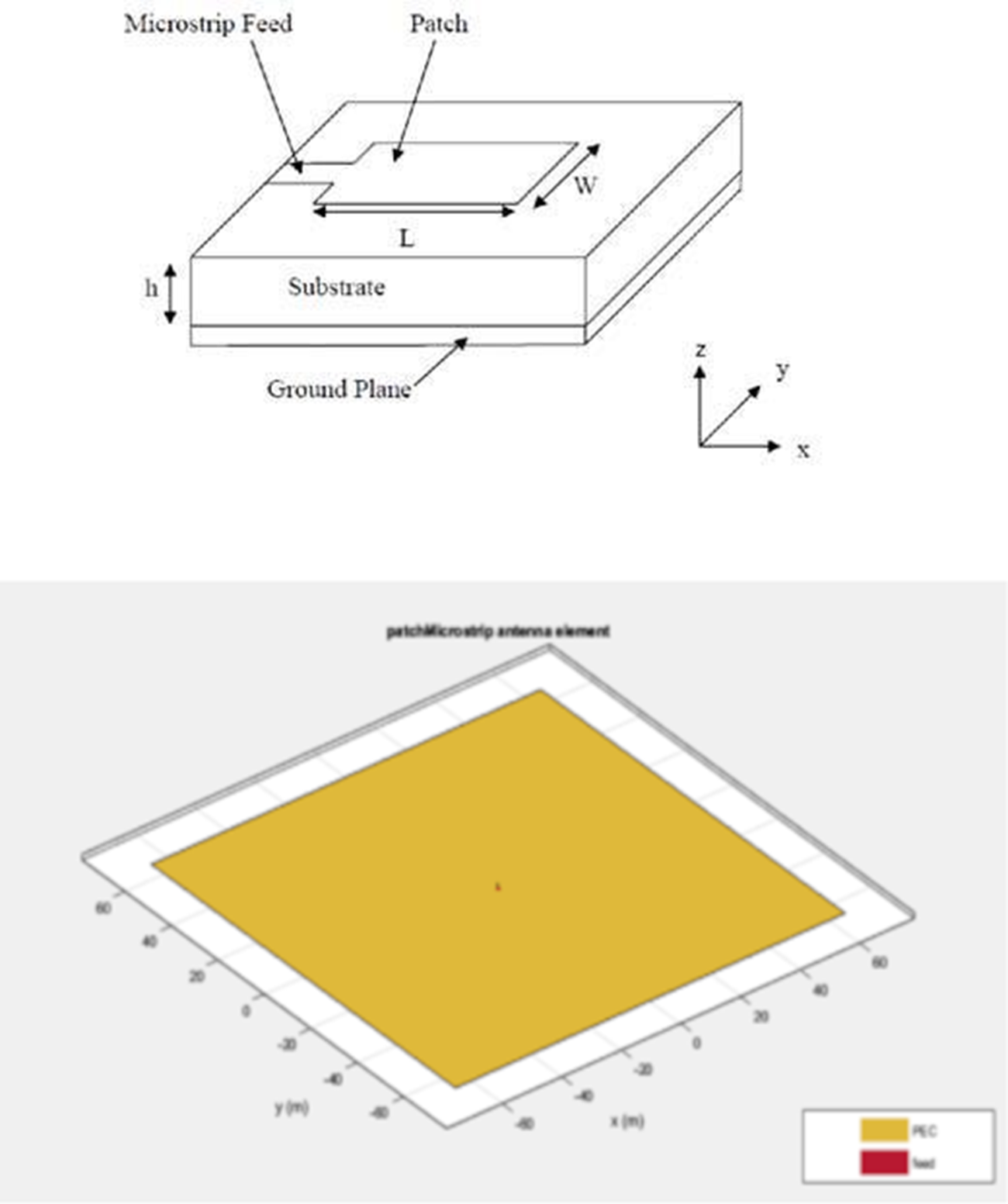
Figure 5. Microstrip patch antenna.

Dataset 3 – bowtie antenna

The bowtie antenna is a simple antenna where the antenna feed is at the center of the antenna. This antenna is also called butterfly antenna or a biconical antenna. The angle between the two metal pieces (D) is dependent on the length and width of the antenna and is calculated by the equation.

(1)\begin{equation}D = 2 \times a\,\tan \left( {L/W} \right)\end{equation}

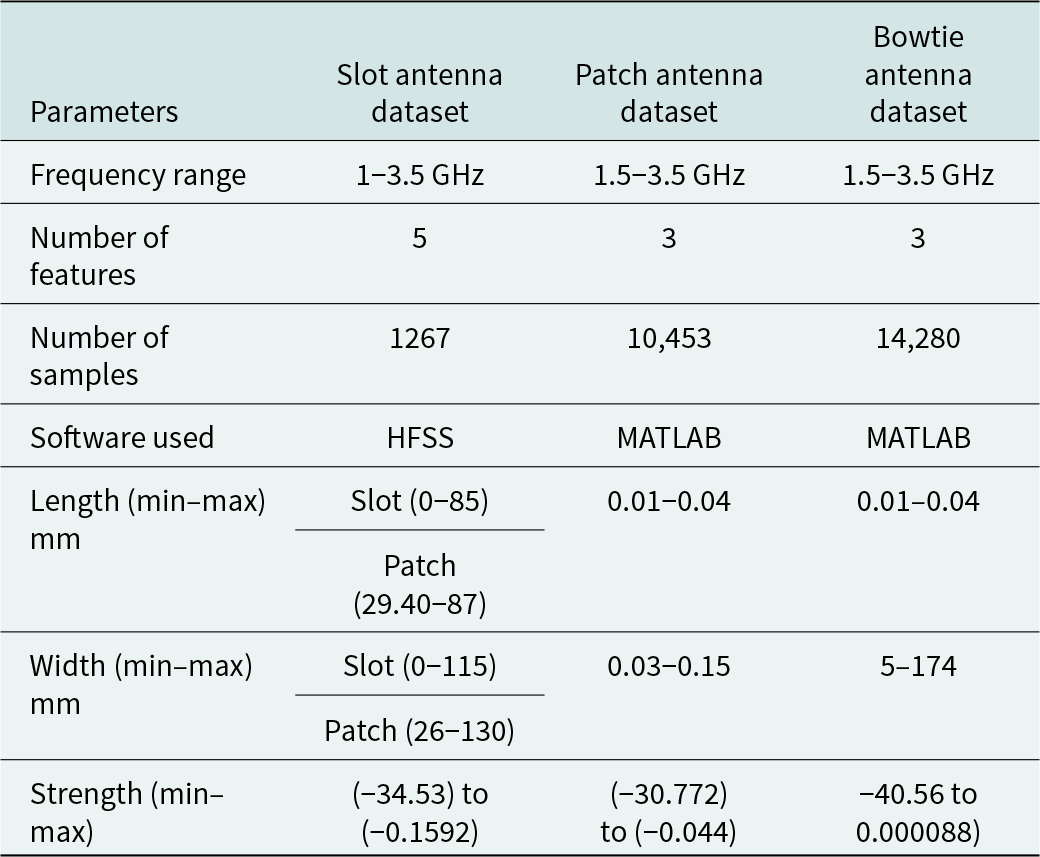
The bowtie antenna dataset consists of a total of 14,280 samples. This dataset also consists of three features (length, width, and frequency) as a design parameter. This dataset was also generated using MATLAB Simulink Antenna Toolbox. The length and width of the bowtie antenna were varied by increasing by 0.01 mm from 0 to a maximum value of 4 mm. The frequency also varied from 0.1 GHz in a range from 1.5 to 3.5 GHz. For each combination of these inputs, the signal strength was simulated for the bowtie antenna. All other parameters were kept to their default value during simulation in MATLAB. Figure 6 [Reference Balanis39] shows the general structure of the bowtie antenna. Table 1 shows a detailed comparison between these three datasets.

Figure 6. Planar bowtie antenna.

Table 1. Comparison of different parameters of three antenna datasets

Evaluation metrics

To evaluate the performance of our ML models, we used two popular evaluation metrics: root mean square error (RMSE) score and R-squared (R ² or coefficient of determination) score, to measure the model performance in our testing data. In both these evaluation metrics, the target value is compared with the actual value to analyze the performance of the machine learning algorithms. RMSE metrics tell us about the average distance between the predicted and actual values and is calculated as:

(2)\begin{equation}{\textrm{RMSE}} = \sqrt {\mathop \sum {{\left( {{P_i}^2 - {Q_i}^2} \right)}^2}/n} \end{equation}

where ∑ is summation, P_i is the predicted value for ith observations, Q_i is the observed value for the ith observations, and N is the sample size.

R ² represents the proportion of the variance for a dependent variable that is explained by an independent variable or variable in a regression model. It measures how well the regression line approximates the actual data. The variance can be calculated as

(3)\begin{equation}{{\textrm{R}}^2} = 1 - {{\rm sum\, squared\, regression\left( {SSR} \right)} \over {\rm total\, sum\, of\, square\left( {SST} \right)}}\end{equation}

(4)\begin{equation}{R^2} = 1- \frac{ {\sum _{i = 1}^n{{\left( {{y_i} - \hat y} \right)}^2}}} {{\sum_{i = 1}^n{{\left( {{y_i} - \widehat {\bar y}} \right)}^2}}}\end{equation}

where y_i = actual y value, $\hat y$ = predicted y value, and $\widehat {\bar y}$ = mean of y value.

Experiments/results

Our preliminary results show that there is a great possibility to utilize machine learning algorithms to optimize the design of an antenna. Table 2 shows the results for the RMSE score and R ² value for different ML algorithms for all three antennae. For slot antenna, RF, GB, and KNN have the top three performances with 0.4087, 0.7484, and 0.3752 RMSE values, respectively. Similarly, for the microstrip patch antenna, RF, BR, and XGB are the top three performers. Each has an R ² value of 99.83%. For the bowtie antenna, RF with a 0.959, BR with 0.5889, and XGB with a 0.7712 RMSE scores are the top three performers. For all antenna datasets, RF is in the top three for all the antenna datasets. SGD regressor and SVR have the lowest performance among all regression methods. As we have used optimization techniques for selecting the optimal hyperparameters for each model, most of the models’ performance has improved, decreasing the RMSE scores.

Table 2. RMSE and R ² values for all the ML algorithms for all antennae

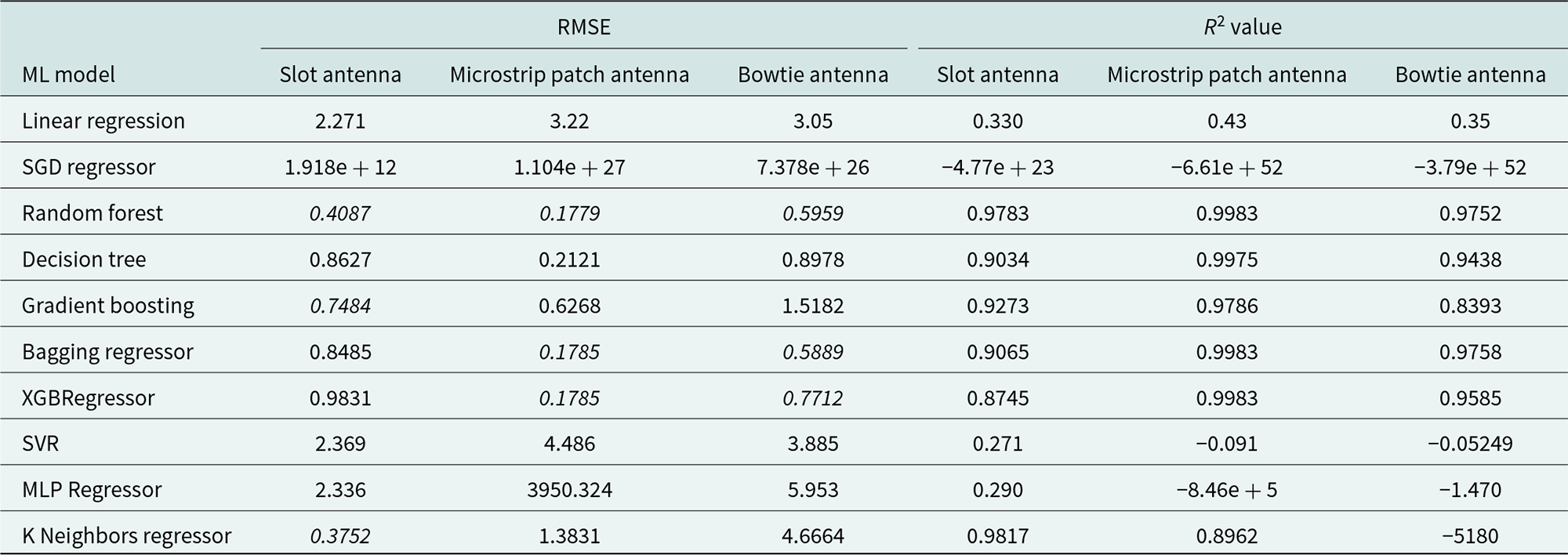
Table 3 shows the scatter plot of the actual strength and predicted strength for different dimensions of different antennae for different ML algorithms. From the figure, we can see that the points are gathered near the regression line in RF, DT, GB, BR, and XGB, which have higher performance and low RMSE score. This shows that these ML models can correctly predict the strength of an antenna based on the input dimension parameters. The point is scattered far away from the regression line in other ML algorithms. This shows that this model has not been able to learn much from the training data and is not suitable for the prediction for these kinds of dataset with these input features. These models may improve the performance of the dataset with different features, along with changing the model parameters for better prediction.

Table 3. Scatter plot for all the ML algorithms for three antennas

Table 4 provides the performance evaluation using 10-fold CV methods. This table shows the average (mean score) of the RMSE score and standard deviation of all 10 iterations. In the 10-fold CV also, RF has shown great performance for slot antenna and bowtie antenna, whereas XGBregressor has the highest performance for the patch antenna. Also, apart from some scores, the CV score is quite like the individual ML performance where we have divided the whole dataset into training and testing datasets. This also shows the uniformity of the model performance and removes the overfitting of data while training the model.

Table 4. Mean score and standard deviation using CV methods

Table 5 shows the RMSE score and R ² value for the four ensemble methods which use the top three performers from approach 1. For the analysis of slot antenna, we used RF, GB, and KNN regressor models, whereas for patch antenna and bowtie antenna, we used RF, BR, and XGB regressor as they are the top three highest performing models among all the ML models. Blending methods has shown a very good performance in slot antenna (having an R ² value more than 98%). All the ensemble methods have shown a comparable result in patch antenna, where R ² value is more than 99% in all the methods. Similarly, blending method has proved to be better with more than 99% of R ² value for bowtie antenna as compared to other ensemble methods. It shows that using these methods, more than 99% of the variation in the predicted values is accounted for by the input parameters of the antenna. Also, looking at the performance of the patch antenna and bowtie antenna as compared to the slot antenna, the number of data points has shown great importance in the prediction performance. With larger number of sample size in patch antenna and bowtie antenna as compared to very small sample size in slot antenna, experiment shows that increasing sample size can increase the prediction accuracy. This may be because more sample points provide more information about the data and therefore provide better estimation results with higher probability of convergence while training the model.

Table 5. RMSE and R ² results for all the ensemble models for all our datasets

Table 6 shows the scatter plot using the ensemble methods for all three antennas. Apart from some outliers which are very far away from the regression line, we can see that most of the points are grouped near the regression line showing the accurate prediction of the antenna strength as compared to the actual values from the dataset.

Table 6. Scatter plot for all the ensemble ML algorithms for three antennas