


Introduction
Palmer amaranth (Amaranthus palmeri S. Watson) is the most troublesome weed in agronomic cropping systems in the United States (Heap Reference Heap, Pimentel and Peshin2014). Several factors have enabled A. palmeri to become such a dominant and difficult-to-control weed, including its rapid growth rate (Ehleringer Reference Firbank and Watkinson1985; Ehleringer and Forseth Reference Ehleringer and Forseth1980), prolific seed production (Keeley et al. Reference Keeley, Carter and Thullen1987), and ability to tolerate adverse environmental conditions (Franssen et al. Reference Franssen, Skinner, Al-Khatib, Horak and Kulakow2001), including disease, genetic abnormalities, and water stress (Chahal et al. Reference Chahal, Irmak, Jugulam and Jhala2018). From a 2-yr field study in Kansas, Horak and Loughin (Reference Horak and Loughin2000) reported that A. palmeri had a 50% higher growth rate (i.e., 0.18 to 0.21 cm per growing degree day) and leaf area than redroot pigweed (Amaranthus retroflexus L.), tumble pigweed (Amaranthus albus L.), and waterhemp [Amaranthus tuberculatus (Moq.) Sauer]. In a field trial in Missouri, Sellers et al. (Reference Sellers, Smeda, Johnson, Kendig and Ellersieck2017) reported a 65% greater dry weight of A. palmeri compared with A. retroflexus and A. albus, A. tuberculatus, spiny amaranth (Amaranthus spinosus L.), and smooth pigweed (Amaranthus hybridus L.) 2 wk after planting. It has also been reported that A. palmeri has greater root length and root biomass than most crops, allowing it to occupy a larger soil volume and extract soil nutrients (Wright et al. Reference Wright, Jennette, Coble and Rufty1999), leading to crop yield losses if it is not controlled early in the growing season. Annually, weeds cause an estimated economic loss of more than US$100 billion and a 10% yield loss on a global scale (Appleby et al. Reference Appleby, Muller, Carpy and Muller2000). In light of these losses, it is clear that a greater understanding of crop–weed interactions in terms of water, nutrients, light, and competition for other resources is necessary to develop cost-effective and sustainable weed management practices.
Crop–weed competition models offer a significant tool for understanding and predicting crop yield losses due to crop–weed interference. Research is currently dominated by empirical studies in which crop yield loss (or crop yield) and weed threshold values are predicted in response to variable weed density or biomass in certain environmental conditions. Complex empirical models have been developed by considering variables such as multiple weed species in simultaneous competition (Diggle et al. Reference Diggle, Neve and Smith2003; Firbank and Watkinson Reference Firbank and Watkinson1985; Pantone and Baker Reference Pantone and Baker1991; Park et al. Reference Park, Benjamin and Watkinson2002), timing of weed emergence (Cousens et al. Reference Cousens, Brain, O’Donovan and O’Sullivan1987; Neve et al. Reference Neve, Diggle and Smith2003), and weeds with multiple emergence patterns (Peltzer et al. Reference Peltzer, Dougla, Diggle, George and Renton2012). However, within these models, weed biological characteristics are unknown, limiting our understanding of weed growth in competition with crops and how that competition affects crop growth parameters as well as soil water dynamics and water use (evapotranspiration).
At the intersection of weed and crop stomatal behavior, environmental conditions, and soil water availability, evapotranspiration is a major unknown. Crop–weed competition is a complex phenomenon, and for predictive purposes, a detailed mechanistic model offers greater insights than an empirical model. Mechanistic models consider all underlying morphological and physiological processes and their dependence on one another with respect to external forces and time (Singh et al. Reference Singh, Kaur, Chauhan, Chantre and Gonzalez-Andujar2020). However, morphological and physiological plasticity in weed species is a challenge for studies/models that have been developed based on weed growth. Although some research on weed biology and ecology has been conducted, additional systemic studies in different locations and under different environmental conditions are needed to elucidate simulation models and thus weed management decisions (Chauhan and Johnson Reference Chauhan and Johnson2010; Van Acker Reference Van Acker2009). Robustly measured evapotranspiration data in systems can aid in strengthening modeling capabilities.
In terms of crop–weed competition, the competitive ability of crops depends on many factors, such as (1) crop type and cultivar or variety selection, sowing date, row spacing, and tillage practice; (2) weed density and composition; (3) soil and climatic factors; and (4) crop rotation (Singh et al. Reference Singh, Kaur, Chauhan, Chantre and Gonzalez-Andujar2020). As the inherent ability of crops to compete against weeds is weakened by climatic and soil stresses (Mohler Reference Mohler, Liebman, Mohler and Staver2004), the time and method of irrigation management may also impact crop–weed competition, as weeds also benefit from increases in available soil water during irrigation. Additionally, understanding when, where, and how water is consumed by evapotranspiration is useful not only for evapotranspiration analyses, but for improving water use efficiency.
Developing irrigation management strategies based on available soil water requires knowledge of weed and crop responses to water deficits, which can be obtained through modeling (Paredes et al. Reference Paredes, Rodrigues, Alves and Pereira2014), relating biomass production to actual evapotranspiration (ETa). The effects of crop ETa rates on crop yield are well known; however, there is a lack of scientific information in terms of the effect of weed ETa on weed morphological features (e.g., biomass, leaf area index, plant height). While empirical crop–weed competition models have been useful, they have not been adequate in predicting crop–weed competition with A. palmeri under varying irrigation practices. By adopting a mechanistic approach to examine the effects of irrigation type on A. palmeri and crop competition, we can begin to use parameters such as ETa and total soil water (TSW) to strengthen predictive capabilities of mechanistic crop–weed competition models. Thus, the objective of this research was to determine the effect of center-pivot (CPI) versus subsurface drip irrigation (SDI) systems on the ETa of A. palmeri grown in maize (Zea mays L.), soybean [Glycine max (L.) Merr.], and fallow systems under the soil, climate, crop, and water management conditions of south-central Nebraska.
Materials and Methods
Plant Materials
Glyphosate-resistant A. palmeri seeds were germinated in 11.4-cm-deep square plastic pots in a University of Nebraska–Lincoln greenhouse maintained at 18/24 C day/night temperatures with a 14-h photoperiod. Glyphosate-resistant A. palmeri was used so that other weeds could be controlled after A. palmeri plants were transplanted in the field. To ensure that A. palmeri plants were glyphosate-resistant, glyphosate at 2,526 g ae ha−1 mixed with liquid ammonium sulfate at 3% v/v was sprayed on 10- to 12-cm-tall A. palmeri plants using an AIXR TeeJet® (TeeJet, Grime, IA) nozzle. The herbicide mixture was applied at a rate of 140.3 L ha−1 at 1.0 m s−1 using a chamber track sprayer. Amaranthus palmeri plants survived the glyphosate application, signifying that the seed source was truly glyphosate resistant.
Field Experimental Design, Site Description, and Crop Management
Field experiments were conducted in 2019 and 2020 growing seasons in the Irmak Research Laboratory’s advanced crop production, evapotranspiration, irrigation engineering, plant physiology, and climate change impact on agriculture and water resources research facilities at the University of Nebraska–Lincoln, South Central Agricultural Laboratory near Clay Center, NE (40.57°N, 98.12°W). A large experimental field was divided into CPI and SDI research facilities, both of which irrigation methods were established/installed by the senior author (SI) in 2005. Thus, the field topography, slope, soil characteristics, and other soil- and field-related characteristics of both CPI and SDI fields were similar (Table 1). The CPI field was irrigated using a four-span hydraulic and continuous-move system (T-L Irrigation, Hastings, NE) (Irmak Reference Irmak2015). In the SDI field, 257-m-long drip lines were installed 0.40 m below the soil surface and were centered in the interrow area of every other plant row. Irrigation was applied directly to the crop root zone via drip emitters spaced approximately 0.45 m apart along the drip lines (Netafim-USA, Fresno, CA) (Irmak Reference Irmak2010). Typical effective rooting depth of field maize in the experimental site is 1.2 m. The 30-yr average rainfall in the area during the growing season (May to August) is 112.4 mm, with significant annual and growing season variability in both timing and magnitude (de Sanctis and Jhala Reference De Sanctis and Jhala2021; Irmak Reference Irmak2010, Reference Irmak2015). Rainfall data from the 2019 and 2020 growing seasons are presented in Figure 1.
Table 1. Field and soil characteristics of center-pivot and subsurface drip irrigation fields.


Figure 1. Daily rainfall in (A) 2019 and (B) 2020 growing seasons at the experimental site (University of Nebraska–Lincoln, South Central Agricultural Laboratory near Clay Center, NE).
The experiment was carried out as a split-plot design with two levels of irrigation assigned at the whole-plot level: CPI and SDI. At the split-plot level, six crop types were assigned to subplots. Nonrandomized subplots consisted of maize, soybean, and no crop (i.e., fallow) with A. palmeri; and maize, soybean, and fallow without A. palmeri. Maize, soybean, and fallow subplots without A. palmeri were included for TSW and actual evapotranspiration (ETa) data comparisons with subplots containing A. palmeri. Each subplot measured 3-m wide by 9-m long, with four rows of maize or soybean in the subplots containing these crops. The field was rolling stalk-chopped without tillage. A broadcast application of 11-52-0 N-P-K at 168 kg ha−1 and an in-furrow injection of 32-0-0 N-P-K at 201 kg ha−1 were applied across the entire experimental site before crops were sown. ‘Dekalb DKS 60-87RIB’ maize was planted at a depth of 5.0 cm and rate of 85,000 seeds ha−1. ‘NK S29-K3X’ soybean was planted at a depth of 3.8 cm and rate of 375,000 seeds ha−1.
Once A. palmeri plants reached a height of 18 to 25 cm in the greenhouse, 12 plants were alternately transplanted 1 m apart in the two center rows of the subplots assigned A. palmeri. A premix of saflufenacil–imazethapyr–pyroxasulfone (Zidua® PRO herbicide) (Zidua Pro herbicide, Research Triangle Park, NC) (Acuron herbicide, Greensboro, NC) was applied at 215 g ai ha−1 to soybean; a premix of atrazine–bicyclopyrone–mesotrione–S-metolachlor (Acuron® herbicide) was applied at 2.4 kg ai ha−1 to maize and fallow; and a postemergence application of glyphosate at 1,263 g ha−1 was applied across all plots for control of existing weeds.
Measurement of Soil Water Status and Irrigation Management
Watermark Granular Matrix Sensors (Irrometer, Riverside, CA) were installed next to three A. palmeri plants or crop plants and between three A. palmeri and crop plants in each subplot to measure soil matric potential (SMP) on an hourly basis. The sensors were buried at 0- to 0.30-m, 0.30- to 0.60-m, and 0.60- to 0.90-m soil depths, and hourly data were collected from the A. palmeri transplant date to shortly before crop harvest in both years. A total of 45 and 54 sensors were installed across the subplots of each irrigation system in 2019 and 2020, respectively. The sensors were connected to model 900M Watermark Monitor data loggers (Irrometer). SMP measurements were converted to percent volumetric soil water content (VWC) using predetermined soil water retention curves for the same experimental field (Irmak Reference Irmak2019a, Reference Irmak2019b): ${{\rm{\theta }}_{\rm{v}}} = \left( {3 \times {{10}^{ - 6}} \times {\rm{SM}}{{\rm{P}}^2}} \right) - \left( {0.0013 \times {\rm{SMP}}} \right) + 0.3764$
where θv is the VWC (% vol or m3 m−3), and SMP is the soil matric potential (kPa). VWC was converted to TSW by adding the VWC values at each sensor depth and multiplying by a conversion value of 3.048 (ft to mm). The TSW in the complete monitored soil profile (0 to 0.90 m) reflects the daily integration of soil moisture detected at individual incremental depths throughout the profile. Sensor data were used to determine crop and A. palmeri evapotranspiration using the soil water balance approach and for irrigation timing. Irrigation was initiated under CPI and SDI when the average SMP values of the top 0.90 m were approximately 100 to 110 kPa (Irmak et al. Reference Irmak, Burgert, Yang, Cassman, Walters, Rathje, Payero, Grassini, Kuzila, Brunkhorst, Eisenhauer, Kranz, VanDeWalle, Rees and Zoubek2012, Reference Irmak, Payero, VanDeWalle, Rees, Zoubek, Martin, Kranz, Eisenhauer and Leininger2016), which translates to a depletion of soil water in the crop root zone of 40% to 45% below field capacity (Irmak Reference Irmak2019a, Reference Irmak2019b). This SMP range was implemented to prevent water stress. Irrigation of 32 mm was applied once per experimental field between July 31 and August 2 of 2019. In 2020, irrigation of 32 mm was applied six times per experimental field between July 13 and September 1.
Seasonal Actual Evapotranspiration Using Soil–Water Balance
Crop and A. palmeri actual evapotranspiration (ETa, mm) were calculated for each experimental subplot using the procedures outlined in Irmak (Reference Irmak2015) by implementing a soil water balance equation: $P + I + U + {R_{{\rm{on}}}} = {R_{{\rm{off}}}} + D + \Delta SWS + E{T_a}$
where P is precipitation (mm), I is irrigation water applied (mm), U is upward soil-moisture flux (mm), R on is surface run-on within the field (mm), R off is surface runoff from individual treatments (mm), ΔSWS is change in soil water storage in the root zone soil profile (mm), and D is deep percolation below the crop root zone (mm). U was assumed to be zero, as the groundwater depth in the experimental field is about 33 to 35 m below the surface (Irmak Reference Irmak2010). Deep percolation was estimated by a soil water balance approach using a program written in Microsoft Visual Basic (Bryant et al. Reference Bryant, Benson, Kiniry, Williams and Lacewell1992; Irmak Reference Irmak2015). Inputs to the program include initial water content of the soil profile at crop emergence, irrigation date and amount, maximum rooting depth, crop maturity date, soil parameters, and daily weather data (i.e., incoming shortwave radiation, relative humidity, air temperature, precipitation, and wind speed). The program calculated daily ETa and the water balance in the crop root zone using the two-step approach (ETa = K c × ET0), where ETo is evapotranspiration of a grass reference crop, and K c is the crop coefficient. In the program, ETo is calculated using weather data as the input to the Penman-Monteith equation (Monteith Reference Monteith1965), and K c is used to adjust the estimated ETo for the reference crop to that of the desired crops at different growth stages and environments (Irmak Reference Irmak2015). The daily soil water balance equation used for calculating deep percolation as presented in Irmak (Reference Irmak2015) is: ${D_j} = \max \left( {{P_j} - {R_j} + {I_j} - {\rm{E}}{{\rm{T}}_{{\rm{a}}j}} - {\rm{C}}{{\rm{D}}_{j - 1}},0} \right)$
where D j is deep percolation on day j (mm), P j is precipitation on day j (mm), R j is precipitation and/or irrigation runoff from the soil surface on day j (mm), I j is irrigation depth on day j (mm), ETaj is crop or A. palmeri actual evapotranspiration on day j (mm), and CD j is root zone cumulative depletion depth at the end of day j − 1, estimated using the two-step approach (Irmak Reference Irmak2015). Following Irmak (Reference Irmak2015), R off from individual treatments was estimated using the USDA-NRCS curve number method. As suggested by Irmak (Reference Irmak2015), according to the silt loam soil at the experimental site and the known land use, slope, and conservation tillage, curve number C = 75 was used. Assuming U and R on are negligible, the soil water balance equation was reduced to the following form for calculating crop and A. palmeri ETa (Irmak Reference Irmak2015): ${\rm{E}}{{\rm{T}}_a} = P + I - {R_{{\rm{off}}}} - D \pm \Delta {\rm{SWS}}$
Growth Index, Plant Biomass, and Total Leaf Area Measurements
Three A. palmeri plants were selected and sampled at four removal timings according to soybean growth stage. Soybean growth stage was selected instead of maize growth stage, because it was easier to visually determine compared with maize. Removal timings occurred at V4, R1, R3, and R5 soybean growth stages in 2019, and at R1, R3, R5, and R6 soybean growth stages in 2020. The later removal timings in 2020 were a result of COVID-19 delays. Growth index, plant biomass, and total leaf area of each A. palmeri plant were determined at these removal timings and then averaged over all subsampled replicates for a total of 24 sample units each growing season. Growth index was calculated using the following equation (Irmak et al. Reference Irmak, Haman, Irmak, Jones, Campbell and Crisman2004; Sarangi et al. Reference Sarangi, Irmak, Lindquist, Knezevic and Jhala2015): ${\rm{GI\;}}\left( {{\rm{c}}{{\rm{m}}^3}} \right){\rm{\;}} = {\rm{\;\pi \;}}\times{\rm{\;}}{(w/2)^2}{\rm{\;}}\times{\rm{\;}}h$
where w is the width of the plant calculated as an average of two widths, one measured at the widest point and another at 90° to the first; and h is the plant height measured from the soil surface to the shoot apical meristem. After plant height and width measurements were taken, leaves were counted and removed from each A. palmeri plant to measure total leaf area using a leaf area meter (LI-3100C Area Meter, Li-Cor, Lincoln, NE). Amaranthus palmeri plants were stored separately in paper bags and oven-dried at 65 C for 7 d to obtain dry biomass.
Statistical Analysis
TSW, ETa, growth index, plant biomass, and total leaf area (TLA) responses were averaged over all subsampled replicates across study years. Data responses were averaged across study years, because crop type and A. palmeri combinations were not randomized across subplots. Thus, A. palmeri plants within each crop subplot were not independent replications. When data were averaged across study years, the crop subplots with and without A. palmeri were the experimental units for TSW and ETa data analyses, while sampling date was the experimental unit for growth index, plant biomass, and TLA data analyses.
Response analyses were run in PROC GLIMMIX within SAS v. 9.4 (SAS Institute, Cary, NC). TSW and ETa responses were assumed to be normally distributed based on the residual plots. Variables included in the model were irrigation, crop type, presence of A. palmeri, and time of season in which the treatment response was measured. The time of season variable was created by separating dates across study years into early-, mid-, and late-season time intervals (Table 2). Within each time interval, five and four individual dates were included in 2019 and 2020, respectively. Individual dates were used as the level of replication for each of the irrigation, crop type, A. palmeri, and time of season variable combinations. Random effects included in the model accounted for whole-plot variation within a year between experimental units where irrigation was assigned; for split-plot variation due to the relationship between subplots; for variation between the time of season data that were measured within subplots throughout the experiment; and to fit a covariance structure to the residual variability that arose from the relationship between individual date measurements taken on the same experimental units within combinations of year, irrigation, crop type, and time of season. AR(1) and ARH(1) structures were utilized for the TSW and ETa responses, respectively. Least-squares means (LSM) analyses were performed on means of each main effect (i.e., irrigation, crop type, presence of A. palmeri, and time of season) across years. A t-test was performed for all LSM analyses to indicate differences among the estimated means of the main effects.
Table 2. Early-, mid-, and late-season date ranges within each time interval in 2019 and 2020.

Growth index, plant biomass, and TLA subsampled averages were skewed, with late-season responses having much larger values than early- and mid-season treatment responses. Based on the skewness and the fact that these treatment responses can only have values greater than zero, the responses were analyzed using a gamma distribution with a log link function (Lawless Reference Lawless2002; Nelson Reference Nelson1982). Final analyses for growth index, plant biomass, and TLA contained 48 observations, including data across 2 yr, two types of irrigation, three crop types, and four sampling dates. Averaging over the subsamples, year measurements were used as the level of replication; thus, variables included in the final model were irrigation, crop type, and sampling date. The model contained random effects accounting for whole-plot variation within a year between experimental units where irrigation was assigned and for split-plot variation due to the relationship between subplots.
Results and Discussion
TSW
Regarding the time of season effect, early-season TSW was greatest (308 mm), followed by similar midseason (288 mm) and late-season (290 mm) subsampled TSW means (Figure 2B). Neither irrigation method nor presence of 1 A. palmeri plant m−2 significantly affected TSW at the subplot level. Although 1 A. palmeri plant m−2 did not significantly affect mean subplot TSW in this study, it is plausible that A. palmeri density > 1 plant m−2 will have variable effects on TSW given differing environmental conditions (Nielsen et al. Reference Nielsen, Lyon, Higgins, Hergert, Holman and Vigil2016; Robinson and Nielson Reference Robinson and Nielsen2015; Unger and Vigil Reference Unger and Vigil1998). Studies conducted by Berger et al. (Reference Berger, Ferrell, Rowland and Webster2015) and Massinga et al. (Reference Massinga, Currie and Trooien2003) found that crop fields with 1 A. palmeri plant m−2 have lower TSW than weed-free cropping systems. Several factors could have affected these results, including hard to control weeds that impacted subplot water use data (e.g., spotted spurge [Chamaesyce maculata (L.) Small]), low sample size for each treatment, and deeper rooting systems of A. palmeri compared with maize and soybean. Although root length and distribution of A. palmeri plants were not collected, the rooting system of A. palmeri plants likely extended beyond the depth of the soil-moisture sensors in the study (Wright et al. Reference Wright, Jennette, Coble and Rufty1999), increasing the TSW around soil-moisture sensors in fallow subplots with A. palmeri.

Figure 2. Estimated average total soil water (TSW, mm) across (A) crop type and (B) time of season in a study to determine evapotranspiration of Amaranthus palmeri in maize, soybean, and fallow under center-pivot and subsurface drip irrigation systems at the experimental site (University of Nebraska–Lincoln, South Central Agricultural Laboratory near Clay Center, NE). Standard error bars represent a 95% confidence interval. Different letters indicate significant differences between crop type and time of season (P ≤ 0.05).
According to a type III test of fixed effects for variable interactions and main effects, TSW was affected by crop type (P = 0.002) and time of season (P = 0.0023) across 2019 and 2020. Mean TSW was greatest in fallow subplots with and without A. palmeri (325 mm), followed by mean TSW in soybean subplots (291 mm) and maize subplots (269 mm) with and without A. palmeri (Figure 3A). These results were expected, as A. palmeri was the only plant extracting soil water in fallow subplots, while both A. palmeri and crops were extracting soil water in the maize and soybean subplots. These results are also supported by the fact that A. palmeri typically has a deeper root system than maize or soybean (Wright et al. Reference Wright, Jennette, Coble and Rufty1999), allowing A. palmeri to extract soil water far below the soil-moisture sensors, resulting in higher mean TSW in fallow subplots.

Figure 3. Estimated average actual evapotranspiration (ET, mm) across crop type and time of season in a study to determine evapotranspiration of Amaranthus palmeri in maize, soybean, and fallow under center-pivot and subsurface drip irrigation systems at the experimental site (University of Nebraska–Lincoln, South Central Agricultural Laboratory near Clay Center, NE). Standard error bars represent a 95% confidence interval. Different letters indicate significant differences between crop type and time of season (P ≤ 0.05).
Scaled Actual Evapotranspiration
According to a type III test of fixed effects for variable interactions and main effects, ETa was affected by crop type and time of season interaction (P = 0.013) and by the presence of A. palmeri (P = 0.045) across 2019 and 2020. According to the simple effect comparisons of the crop type and time of season interaction, subplots with maize and soybean recorded statistically greater early-season ETa of 28 to 30 mm and late-season ETa of 7 to 8 mm compared with fallow subplots. Midseason subplot ETa values in maize and soybean were similar, while fallow subplot ETa was similar to maize and slightly lower than soybean subplot ETa (Figure 3). Sugita et al. (Reference Sugita, Matsuno, El-Kilani, Abdel-Fattah and Mahmoud2017) reported similar time of season changes of ETa, where strong ETa responses to irrigation or rain events occurred during earlier growth stages, and more stable ETa responses occurred at the vegetative peak of the growing season. This is important, because A. palmeri can germinate and grow throughout an entire growing season (May to September) (Keeley et al. Reference Keeley, Carter and Thullen1987). Although germinating late in the growing season may be detrimental to A. palmeri growth and seed production, optimal temperatures late into the growing season allow for rapid growth of A. palmeri while maize and soybean growth is beginning to slow, increasing the competitive ability of A. palmeri for water and nutrients that the crop also needs for seed production.
Regarding the presence of A. palmeri on ETa, subplots with A. palmeri had greater ETa of 28 mm compared with 23 mm in subplots without A. palmeri (Figure 4). Greater ETa from subplots with A. palmeri can be attributed to the variable relationship between VWC and ETa throughout the growing season (Wilson et al. Reference Wilson, Kustas, Alfieri, Anderson, Gao, Prueger, McKee, Alsina, Sanchez and Alstad2020). In early spring, when V2-V3 crops and 18- to 25-cm A. palmeri were the primary sources of evapotranspiration, ETa was strongly correlated with VWC. As crop and A. palmeri growth progressed, ETa was largely independent of VWC as plants began to access water beyond the depth of the soil-moisture sensors. As the soil profile dried during the growing season, the correlation between ETa and VWC emerged once again as the crop became largely dependent on irrigation. Amaranthus palmeri likely affected overall subplot ETa, because the root system remained below 0.90 m and was less dependent on irrigation compared with the crops. Root length and root distribution of A. palmeri plants were not analyzed in this study, although these plant characteristics likely contributed to the ETa differences seen in subplots with and without A. palmeri (Wright et al. Reference Wright, Jennette, Coble and Rufty1999).

Figure 4. Estimated average actual evapotranspiration (ET, mm) of subplots with and without Amaranthus palmeri in a study to determine evapotranspiration of Amaranthus palmeri in maize, soybean, and fallow under center-pivot and subsurface drip irrigation systems at the experimental site (University of Nebraska–Lincoln, South Central Agricultural Laboratory near Clay Center, NE). Standard error bars represent a 95% confidence interval. Different letters indicate significant differences between subplots with and without A. palmeri (P ≤ 0.05).
Growth Index, Plant Biomass, and TLA
According to a type III test of fixed effects for variable interactions and main effects, the mean growth index and mean biomass of A. palmeri were affected by a sampling date and crop type interaction across both study years (P < 0.0001). As expected, from the second sampling date onward, the growth index and biomass of A. palmeri in fallow subplots were higher (0.3 to 5.6 m3 and 0.06 to 1.27 kg, respectively) compared with A. palmeri in maize (0.06 to 0.23 m3 and 0.008 to 0.03 kg, respectively) and soybean (0.06 to 0.7 m3 and 0.01 to 0.16 kg, respectively) subplots (Figures 5 and 6). While A. palmeri growth index rates in maize and soybean were similar throughout the growing season, A. palmeri biomass was higher in soybean (0.05 to 0.16 kg) compared with maize (0.01 to 0.03 kg) at the third and fourth sampling dates (Figure 6). Mahoney et al. (Reference Mahoney, Jordan, Hare, Leon, Roma-Burgos, Vann, Jennings, Everman and Cahoon2021) reported similar results, wherein taller weeds like A. palmeri were more competitive in fields with shorter crop canopies (e.g., soybean) and less competitive in crops that provide shading earlier in the growing season (e.g., maize), resulting in greater A. palmeri biomass in soybean systems (0.035 kg plant−1) compared with maize systems (0.002 kg plant−1). The reason for this is that when growing in competition with maize, A. palmeri allocates most of its resources toward vertical growth, whereas in competition with soybean, A. palmeri first allocates most of its resources toward vertical growth. Once it reaches the soybean height, A. palmeri begins allocating most of its resources toward lateral growth, resulting in more branching and thus greater biomass production. These results are not surprising, given A. palmeri’s rapid growth rate (Culpepper et al. Reference Culpepper, Webster, Sosnoskie, York and Nandula2010; Horak and Loughin Reference Horak and Loughin2000), biomass accumulation (Sellers et al. Reference Sellers, Smeda, Johnson, Kendig and Ellersieck2017), and photosynthetic rate three to four times that of maize, soybean, and cotton (Gossypium hirsutum L.) (Steckel Reference Steckel2007).

Figure 5. Estimated average of scaled Amaranthus palmeri growth index across crop type within each sampling date in a study to determine evapotranspiration of Amaranthus palmeri in maize, soybean, and fallow under center-pivot and subsurface drip irrigation systems at the experimental site (University of Nebraska–Lincoln, South Central Agricultural Laboratory near Clay Center, NE). Standard error bars represent a 95% confidence interval. Different letters indicate a significant difference between crop types within each sampling date (P ≤ 0.05). Estimates are scaled down by a factor of 100,000 cm3. Date 1: June 20, 2019, July 2, 2020; Date 2: July 2, 2019, July 14, 2020; Date 3: July 18, 2019, August 4, 2020; Date 4: August 8, 2019, August 26, 2020.
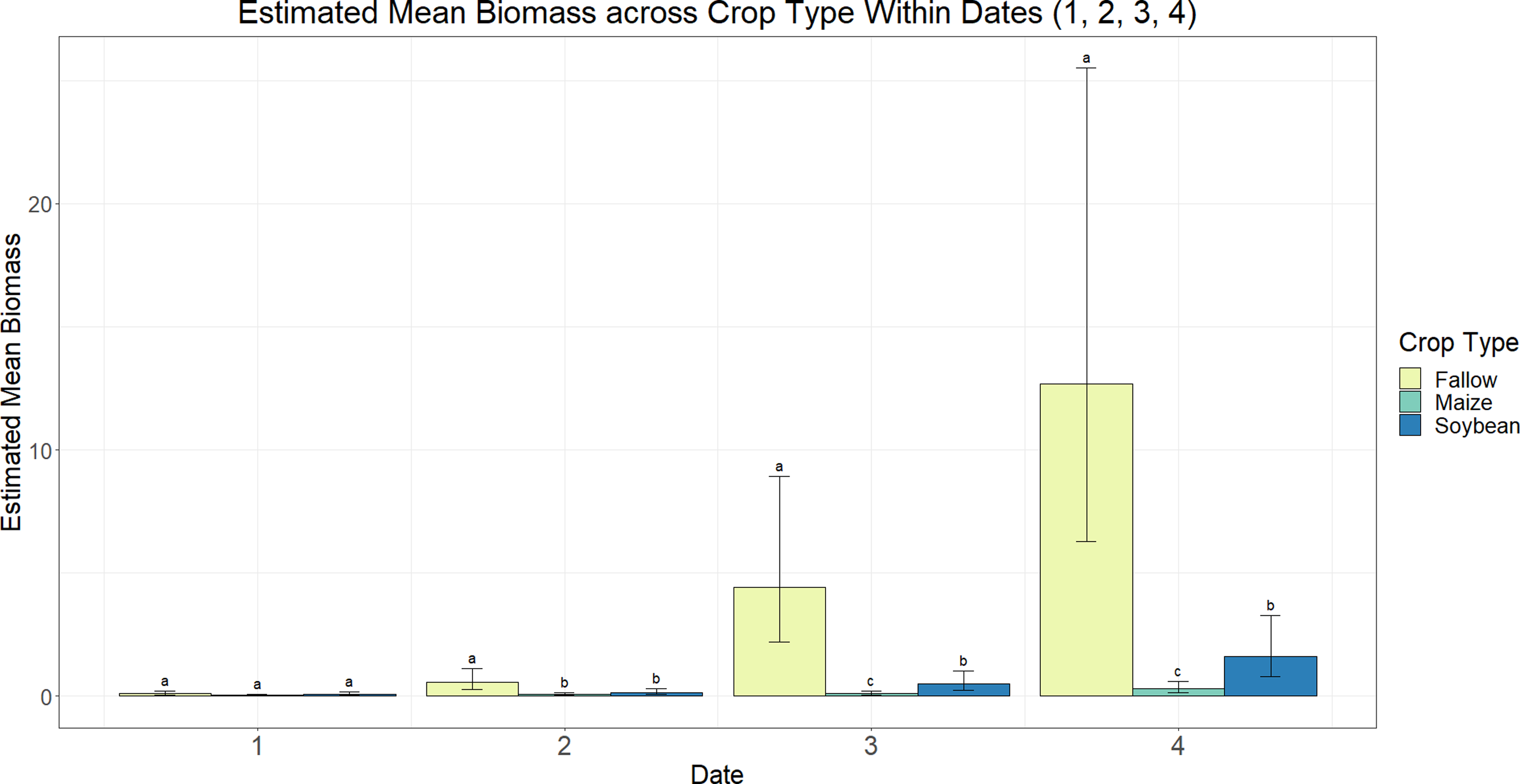
Figure 6. Estimated average of scaled Amaranthus palmeri biomass across crop type within each sampling date in a study to determine evapotranspiration of Amaranthus palmeri in maize, soybean, and fallow under center-pivot and subsurface drip irrigation systems at the experimental site (University of Nebraska–Lincoln, South Central Agricultural Laboratory near Clay Center, NE). Standard error bars represent a 95% confidence interval. Different letters indicate a significant difference between crop types within each sampling date (P ≤ 0.05). Estimates are scaled down by a factor of 100 g. Date 1: June 20, 2019, July 2, 2020; Date 2: July 2, 2019, July 14, 2020; Date 3: July 18, 2019, August 4, 2020; Date 4: August 8, 2019, August 26, 2020.
According to a type III test of fixed effects for variable interactions and main effects, A. palmeri TLA was affected by a sampling date, irrigation, and crop type interaction across both years (P = 0.023). Similar to A. palmeri growth index and biomass results, differences in A. palmeri TLA across crop type were evident from the second sampling date until the end of the growing season. The TLA of A. palmeri in fallow subplots was greater (41 to 2,575 m2) compared with maize (6.6 to 17.8 m2) and soybean (10.0 to 47.6 m2) subplots, which correlates with A. palmeri growth index and biomass results. An irrigation effect on TLA was detected, although this is likely due to the missing TLA data points of A. palmeri in fallow subplots under CPI and SDI in 2020. Due to a severe hailstorm the evening before the sampling date, only one A. palmeri in the fallow subplot under CPI was sampled for TLA in 2020, resulting in skewed A. palmeri TLA under SDI from an outlier in 2019. Thus, sampling date and crop type are the variables more likely to affect TLA in this study.
Practical Implications
This is the first study evaluating the actual evapotranspiration (ETa) of A. palmeri in multiple crops under CPI and SDI with the goal of finding an irrigation effect on A. palmeri ETa. The results indicate differences in A. palmeri ETa between time of season (early, mid-, and late season) and crop species across 2019 and 2020. While our analyses indicate irrigation contributes to differences in mid- and late-season A. palmeri TLA between crop species, irrigation did not affect subplot or sub-subplot ETa, TSW, or A. palmeri growth index or biomass. Additionally, the irrigation effect on A. palmeri TLA is likely a result of missing TLA data at the fourth sampling date in 2020.
Although irrigation did not significantly affect subplot data, the presence of A. palmeri did have an impact on sub-subplot ETa across both years. This can be attributed to the variable relationship between VWC and ETa throughout the growing season due to advancing phenological stages and management practices. As crop and A. palmeri growth progressed, ETa was largely independent of VWC as plants began to access water beyond the depth of the soil-moisture sensors. As the soil profile dried during the growing season, the correlation between ETa and VWC emerged once again as the crop became largely dependent on irrigation. However, A. palmeri likely affected overall sub-subplot ETa, because the root system remained below 0.90 m and was less dependent on irrigation compared with the crops. Root length and root distribution of A. palmeri plants were not analyzed in this study, although these data parameters likely contributed to the ETa differences seen in subplots with and without A. palmeri. Thus, future studies exploring weed species’ water use should measure root length and root distribution using soil-moisture sensors over the entire rooting profile of the plant to better understand the relationship between VWC and ETa. As indicated by the time of season effect on TSW and ETa, irrigation or rain events, along with plant phenotypical development, can significantly influence the TSW and ETa relationship. These observations hold significance for growers who are considering irrigation expansion and upgradation. Selecting an SDI system may lower water use due to reduced evaporation; however, the presence of a heavy A. palmeri infestation in an SDI field may increase competition for water between A. palmeri and the crop, because the irrigated water is more readily available to plants. The rooting depth and distribution of A. palmeri under differing irrigation systems will need to be quantified and compared with water use data to make an accurate assessment of irrigation choice.
Traditionally, crop system suitability, irrigation efficiency, and investment cost are factors that determine selection among CPI and SDI systems. However, results of this study suggest that weed–crop competition should also be considered, making irrigation method selection a holistic process that weighs both biotic and abiotic consequences. This study provides fundamentally critical information on A. palmeri evapotranspiration and its relation to A. palmeri morphological features (e.g., growth index, biomass, and TLA) for future use in mechanistic (and empirical) weed–crop competition models. ETa is highly location specific and is driven by weather, soils, and farm management; thus, further research on ETa of economically important broadleaf and grass weed species should be conducted under diverse environments to build a robust database.
Other economically important weed species such as velvetleaf (Abutilon theophrasti Medik.), common lambsquarters (Chenopodium album L.), and giant foxtail (Setaria faberi Herrm.) in row-crop production would likely result in lower ETa due to lower competitive phenotypes compared with A. palmeri. Root depth and distribution, along with growth rate, are factors that would need to be considered when comparing water use of multiple weed species and the effect of varying irrigation methods on water use. The ETa results for A. palmeri would likely differ in other environments as well, demonstrating the need for more research of this nature conducted in diverse environments. Ehleringer (Reference Ehleringer1983) reported the net rate of A. palmeri photosynthesis is temperature dependent, with the optimum range occurring between 36 C and 46 C. The average daytime temperatures in July and August in south-central Nebraska are 29 C and 30 C, respectively (NCEI 2020). If this same study were conducted in the southern United States, A. palmeri plants would likely have higher rates of ETa because of higher rates of photosynthesis due to higher average temperatures, likely increasing A. palmeri growth index, biomass, and TLA. To effectively build a robust database of the interaction of evapotranspiration (i.e., water use) and morphological features of economically important agronomic weed species, this type of research should be implemented across various and diverse environments.
Acknowledgments
The advanced CPI and SDI systems and fields, soil-moisture sensors and data loggers, and other associated irrigation engineering- and evapotranspiration-related field research components were provided by the senior author (SI) in the Irmak Research Laboratory. The authors acknowledge Matt Drudik, Adam Leise, Shawn McDonald, William Neels, Jose de Sanctis, Irvin Schleufer, and Jared Stander for their invaluable assistance on this project. This research received no specific grant from any funding agency or the commercial or not-for-profit sectors. No conflicts of interest have been declared by the authors. The commercial names of the products are provided solely for the readers’ information and do not provide an endorsement or recommendation by the authors or their institutions.


 Open access