


1. Introduction
It is known that the approximation of probability distribution is a fundamental problem in statistical data analysis. The maximum entropy principle proposed by Jaynes [Reference Jaynes22] gives us a general method of approximating a probability distribution. It states that the least biased probability distribution that describes a partially known system is the probability distribution having maximum entropy in the class of all distributions compatible with the available information. Shannon entropy maximization under different constraints has been studied by many researchers. Kapur [Reference Kapur24] and Kagan et al. [Reference Kagan, Linnik and Rao23] gave a maximum entropy characterization for various distributions under moment constraints. Some researchers obtained the distributions that maximize entropy under the constraints on economic inequality measures (for example, see [Reference Eliazar and Sokolov17, Reference Khosravi Tanak, Mohtashami Borzadaran and Ahmadi26, Reference Khosravi Tanak, Mohtashami Borzadaran and Ahmadi27, Reference Ryu and D.35]).
The modeling and analysis of lifetime data play an important role in a wide variety of scientific and technological fields such as engineering, medicine, and biological sciences. In the last decades, a considerable amount of studies were devoted to the introduction of lifetime distributions that provide an adequate fit to real lifetime data. Many models have been introduced in the literature by extending the Weibull and exponential distributions (for example, see [Reference Barreto-Souza, Santos and Cordeiro8–Reference Carrasco, Ortega and Cordeiro10, Reference Lee, Famoye and Olumolade28, Reference Nadarajah and Kotz30, Reference Singla, Jain and Sharma38]). The modeling of lifetime distributions using the maximum entropy principle has been of interest to several researchers. Ebrahimi [Reference Ebrahimi16] suggested some maximum entropy lifetime (MEL) models subject to constraints on the growth and curvature of the hazard function. Asadi et al. [Reference Asadi, Ebrahimi, Hamedani and Soofi4, Reference Asadi, Ebrahimi and Soofi5] developed a maximum entropy procedure using differential inequality constraints for hazard rate function. Distributions with maximum entropy subject to constraints on their L-moments were proposed by Hosking [Reference Hosking21]. Asadi et al. [Reference Asadi, Ebrahimi, Soofi and Zarezadeh6] introduced two new maximum entropy methods for change point modeling of lifetime distribution. Recently, Du et al. [Reference Du, Ma, Wei, Guan and Sun15] proposed a method based on the maximum entropy principle to estimate the hazard rate function.
One of the informative descriptive indices for a random variable X with cumulative distribution function (c.d.f.) F is
 \begin{align}
\eta= \int _0^\infty \bar{F}^{\gamma}(x)\mathrm{d}x,\quad \gamma \geq 1,\end{align}
\begin{align}
\eta= \int _0^\infty \bar{F}^{\gamma}(x)\mathrm{d}x,\quad \gamma \geq 1,\end{align} where  $\bar{F}(x)=1-F(x)$ is called the survival function. η is widely used for measuring concentration, statistical heterogeneity, and randomness, so we name it the general index (GI). In the case γ = 1, GI equals the distribution’s mean. In the case $ \gamma=n $, where n is a natural number, GI coincides with the expected value of the first order statistic $X_{1: n}$ from n independent and identically distributed nonnegative random variables $X_{1}, \ldots, X_{n}$ with survival function $\bar{F}$. There are many applications of order statistics in statistics and applied probability, especially in reliability theory. The extreme order statistic $X_{1: n}$ represents the lifetimes of the series systems. Moreover, there are several applications of extreme values in meteorology (extremes of temperature and pressure), oceanography (waves and tides), aeronautics (gust loads), and hydrology (floods and droughts). For more details on the order statistics, we refer to [Reference Arnold, Balakrishnan and Nagaraja3] and [Reference David and Nagaraja13]. GI also is used to gauge Gini index [Reference Gini20] and generalized Gini index [Reference Donaldson and Weymark14] as measures of heterogeneity and inequality. In addition, some measures of uncertainty and randomness such as cumulative residual Rényi entropy [Reference Sunoj and Linu40] and cumulative residual Tsallis entropy [Reference Rajesh and Sunoj32] are obtained by GI. In this paper, we apply the maximum entropy principle under the constraints on the mean and GI to model lifetime distribution.
This paper is organized as follows. In Section 2, we first review some results on entropy maximization under some moment constraints. Then we derive the maximum entropy distribution subject to the constraints on the mean and GI. Some statistical properties of the obtained distribution and estimation of its parameters by the method of maximum likelihood are studied in Section 3. Also, we perform a simulation study to investigate the performance of the maximum likelihood estimators. Three empirical applications to real data are illustrated in Section 4 to elucidate the potentiality of the proposed model. Finally, the conclusion is provided in Section 5.
2. New maximum entropy distribution
Suppose that X is a random variable having a continuous c.d.f. F with probability density function (p.d.f.) f. Entropy, as a classical measure of information, is defined by
 \begin{eqnarray*}
H(f)=-\int _{-\infty}^\infty f(x)\,\log f(x) \mathrm{d}x,
\end{eqnarray*}
\begin{eqnarray*}
H(f)=-\int _{-\infty}^\infty f(x)\,\log f(x) \mathrm{d}x,
\end{eqnarray*}provided the integral exists. It was originally introduced by Shannon [Reference Shannon37]. In the literature, H(f) is often referred to as the entropy of X or Shannon’s information about F. We refer the reader to [Reference Cover and Thomas11] for more details and references.
The maximum entropy principle is a rational method for determining a consistent probability distribution. It states that among all possible distributions compatible with a given set of constraints, we should choose the one that has maximum entropy. The distribution so obtained is called maximum entropy distribution. Kapur and Kesevan [Reference Kapur and Kesevan25] studied the problem of entropy maximization under the constraints on moments. In other words, by maximizing the Shannon entropy measure subject to the following moment constraints,
 \begin{equation*}
\int_{-\infty}^{\infty} g_{j}(x) f(x) \mathrm{d} x=\mu_{j}, \quad j=0,1, \ldots, m,
\end{equation*}
\begin{equation*}
\int_{-\infty}^{\infty} g_{j}(x) f(x) \mathrm{d} x=\mu_{j}, \quad j=0,1, \ldots, m,
\end{equation*} where  $g_{0}(x)=1$ and $g_{j}(x), j=1, \ldots, m$ are moment functions; $\mu_{0}=1$ and $\mu_{j}, j=1, \ldots, m$ are moment values corresponding to the $g_{j}(x)$ moment function, the p.d.f. of maximum entropy distribution is obtained as follows:
 \begin{equation*}
f(x)=\exp \left(-\lambda_{0}-\sum_{j=1}^{m} \lambda_{j} g_{j}(x)\right),
\end{equation*}
\begin{equation*}
f(x)=\exp \left(-\lambda_{0}-\sum_{j=1}^{m} \lambda_{j} g_{j}(x)\right),
\end{equation*} where  $\exp \left(\lambda_{0}\right)=\int_{-\infty}^{\infty} \exp \left(-\sum_{j=1}^{m} \lambda_{j} g_{j}(x)\right) \mathrm{d} x$ and $\lambda_{1}, \ldots, \lambda_{m}$ are the Lagrange multipliers corresponding to parameters of the maximum entropy distribution. Some well-known distributions such as normal, beta, gamma, exponential, and Weibull can be expressed as maximum entropy distributions, which are obtained under certain moment constraints. For more information on maximum entropy distributions under moment constraints, we refer to [Reference Kapur and Kesevan25, Reference Usta and Kantar41] and references therein.
In this section, we consider the problem of entropy maximization under the constraints on mean and GI. In other words, we intend to solve the problem: Within the class of distributions supported on the nonnegative half-line  $(x \geq 0)$, and possessing a given mean and GI, which is the distribution that maximizes entropy? We answer this question in the next theorem.
Theorem 2.1 The maximum entropy distribution subject to constraints on mean and GI to be µ and η, respectively, has the survival function
 \begin{align}
\bar{F}(x)=\left[{1+\alpha \left(\mathrm{e}^{\beta x}-1\right)}\right]^{-\frac{1}{\gamma-1}},\quad x \geq 0,
\end{align}
\begin{align}
\bar{F}(x)=\left[{1+\alpha \left(\mathrm{e}^{\beta x}-1\right)}\right]^{-\frac{1}{\gamma-1}},\quad x \geq 0,
\end{align}where α and β are positive parameters and depend on µ and η from the constraints.
Proof. The maximization problem is equivalent to minimize the convex functional
 \begin{align*}
\int _0^\infty f(x)\,\log f(x) \mathrm{d}x
\end{align*}
\begin{align*}
\int _0^\infty f(x)\,\log f(x) \mathrm{d}x
\end{align*}subject to the constraints
 \begin{align*}
\begin{cases}
\int _{0} ^\infty f(x) \mathrm{d}x=1, \\ \int _{0} ^\infty xf(x) \mathrm{d}x=\mu , \\ \int _0^\infty \bar{F}^{\gamma}(x)\mathrm{d}x=\eta .
\end{cases}
\end{align*}
\begin{align*}
\begin{cases}
\int _{0} ^\infty f(x) \mathrm{d}x=1, \\ \int _{0} ^\infty xf(x) \mathrm{d}x=\mu , \\ \int _0^\infty \bar{F}^{\gamma}(x)\mathrm{d}x=\eta .
\end{cases}
\end{align*}The corresponding Lagrangian is given by
 \begin{align*}
L(f,\bf{\lambda}) =\int _0^\infty f(x)\,\log f(x)\mathrm{d} x+\lambda _1 \left(\int_{0}^{\infty} f(x)\mathrm{d} x-1\right) \\+\lambda _2 \left(\int_{0}^{\infty} x f(x)\mathrm{d} x-\mu\right)+\lambda _3 \left(\int _0^\infty \bar{F}^{\gamma}(x)\mathrm{d} x-\eta \right),
\end{align*}
\begin{align*}
L(f,\bf{\lambda}) =\int _0^\infty f(x)\,\log f(x)\mathrm{d} x+\lambda _1 \left(\int_{0}^{\infty} f(x)\mathrm{d} x-1\right) \\+\lambda _2 \left(\int_{0}^{\infty} x f(x)\mathrm{d} x-\mu\right)+\lambda _3 \left(\int _0^\infty \bar{F}^{\gamma}(x)\mathrm{d} x-\eta \right),
\end{align*} where  $\bf{\lambda}=(\lambda_1,\lambda_2,\lambda_3)$ is the vector of Lagrange multipliers. The first variation of the Lagrangian $L(f,\bf{\lambda})$ is
 \begin{align*}
\delta[L(f, \bf{\lambda})](\phi)=\lim _{\varepsilon \rightarrow 0} \frac{L(f+\varepsilon \phi, \bf{\lambda})-L(f)}{\varepsilon},
\end{align*}
\begin{align*}
\delta[L(f, \bf{\lambda})](\phi)=\lim _{\varepsilon \rightarrow 0} \frac{L(f+\varepsilon \phi, \bf{\lambda})-L(f)}{\varepsilon},
\end{align*}where ϕ is an arbitrary test function. By some calculations, we have
 \begin{align*}
\delta [L(f,\bf{\lambda})](\phi)=\int _0^\infty \left[1+\log f(x)+\lambda_1+\lambda_2 x+\lambda_3 \left(\gamma \int_{0}^{x} \bar{F}^{\gamma-1}(u)\mathrm{d} u \right)\right]\phi (x)\mathrm{d} x.
\end{align*}
\begin{align*}
\delta [L(f,\bf{\lambda})](\phi)=\int _0^\infty \left[1+\log f(x)+\lambda_1+\lambda_2 x+\lambda_3 \left(\gamma \int_{0}^{x} \bar{F}^{\gamma-1}(u)\mathrm{d} u \right)\right]\phi (x)\mathrm{d} x.
\end{align*} Equating the first variation of the Lagrangian  $L(f,\bf{\lambda})$ to zero yields the following equation:
 \begin{equation}
1+\log f(x)+\lambda_1+\lambda_2 x+\gamma\lambda_3 \int_{0}^{x} \bar{F}^{\gamma-1}(u)\mathrm{d} u =0.
\end{equation}
\begin{equation}
1+\log f(x)+\lambda_1+\lambda_2 x+\gamma\lambda_3 \int_{0}^{x} \bar{F}^{\gamma-1}(u)\mathrm{d} u =0.
\end{equation}Differentiating both sides of Eq. (3) yields the differential equation
 \begin{equation*}
\frac{f^{\prime}(x)}{f(x)}+\lambda _2 +\gamma\lambda _3 \bar{F}^{\gamma-1}(x)=0.
\end{equation*}
\begin{equation*}
\frac{f^{\prime}(x)}{f(x)}+\lambda _2 +\gamma\lambda _3 \bar{F}^{\gamma-1}(x)=0.
\end{equation*}Equivalently,
 \begin{equation}
f^{\prime}(x)+\lambda _2 f(x)+\gamma\lambda _3 f(x)\bar{F}^{\gamma-1}(x)=0.
\end{equation}
\begin{equation}
f^{\prime}(x)+\lambda _2 f(x)+\gamma\lambda _3 f(x)\bar{F}^{\gamma-1}(x)=0.
\end{equation} Using the fact that  $-\bar{F}^{\prime}(x)=f(x)$, we can write Eq. (4) in the following form,
 \begin{align}
-\bar{F}^{\prime\prime}(x)-\lambda _2 \bar{F}^{\prime}(x)-\lambda _3 \left(\bar{F}^{\gamma}(x)\right)^{\prime}=0.
\end{align}
\begin{align}
-\bar{F}^{\prime\prime}(x)-\lambda _2 \bar{F}^{\prime}(x)-\lambda _3 \left(\bar{F}^{\gamma}(x)\right)^{\prime}=0.
\end{align}Integrating both sides of Eq. (5) leads to the Riccati equation:
 \begin{align*}
\bar{F}^{\prime}(x)+\lambda _2 \bar{F}(x)+\lambda _3 \bar{F}^{\gamma}(x)=c,
\end{align*}
\begin{align*}
\bar{F}^{\prime}(x)+\lambda _2 \bar{F}(x)+\lambda _3 \bar{F}^{\gamma}(x)=c,
\end{align*} where c is a constant. Using the fact that  $\bar{F}(x)$ is a survival probability function, we have $\lim_{x\rightarrow \infty}\bar{F}(x)=0$. Consequently, c must be equal to zero. Thus, we arrive at the Bernoulli equation:
 \begin{align}
\bar{F}^{\prime}(x)=c _1 \bar{F}(x)+c _2 \bar{F}^{\gamma}(x),
\end{align}
\begin{align}
\bar{F}^{\prime}(x)=c _1 \bar{F}(x)+c _2 \bar{F}^{\gamma}(x),
\end{align}where c 1 and c 2 are arbitrary real coefficients. The solution of this equation is the survival function
 \begin{align}
\bar{F}(x)=\left[{1+\alpha \left(\mathrm{e}^{\beta x}-1\right)}\right]^{-\frac{1}{\gamma-1}},\quad x \geq 0,
\end{align}
\begin{align}
\bar{F}(x)=\left[{1+\alpha \left(\mathrm{e}^{\beta x}-1\right)}\right]^{-\frac{1}{\gamma-1}},\quad x \geq 0,
\end{align} where α and β are positive-valued parameters. An outline of the derivation of Eq. (7) from the Bernoulli Eq. (6) is given in the Appendix. Since target and constraints functionals are convex, a global maximum is attained at the critical point  $\bar{F}(x)$.
3. Properties of the distribution
3.1. Probability density function and hazard rate
We consider a reparameterization of the model (2) by putting  $\lambda ={1}/({\gamma-1})$ to achieve a parametric model for lifetime distribution with a simpler appearance. So, the c.d.f. of the reparameterized maximum entropy model is given by
 \begin{align}
F(x)= 1-\left[1+\alpha (\mathrm{e}^ {\beta x}-1)\right]^{-\lambda} ,\quad x \gt 0,
\end{align}
\begin{align}
F(x)= 1-\left[1+\alpha (\mathrm{e}^ {\beta x}-1)\right]^{-\lambda} ,\quad x \gt 0,
\end{align} where the parameters α > 0 and λ > 0 control the shapes of the distribution and β > 0 is the scale parameter. We shall refer to the distribution given in (8) as the MEL distribution. If a random variable X has the MEL distribution, then we write  $X \sim {\text {MEL}}(\alpha,\beta,\lambda)$.
The p.d.f. of the MEL distribution takes the form
 \begin{align}
f(x) = \alpha \beta \lambda\, \mathrm{e}^{\beta x}\left[1+\alpha (\mathrm{e}^ {\beta x}-1)\right]^{-\lambda -1} ,\quad \ x \gt 0 .
\end{align}
\begin{align}
f(x) = \alpha \beta \lambda\, \mathrm{e}^{\beta x}\left[1+\alpha (\mathrm{e}^ {\beta x}-1)\right]^{-\lambda -1} ,\quad \ x \gt 0 .
\end{align} The above p.d.f. is asymmetric and skewed. In the range  $\alpha \leq {1}/({\lambda+1})$, the p.d.f. is unimodal and attains its global maximum at the value
 \begin{equation*}
x_{\text {mode }}=\frac{1}{\beta}\,\log \left(\frac{1-\alpha}{\alpha\lambda}\right).\end{equation*}
\begin{equation*}
x_{\text {mode }}=\frac{1}{\beta}\,\log \left(\frac{1-\alpha}{\alpha\lambda}\right).\end{equation*} In the range  $\alpha \gt {1}/({\lambda+1})$, the p.d.f. is monotone decreasing and attains its global maximum at the origin (i.e., $x_{\text {mode }}=0$). At the parameter value α = 1, the p.d.f. (9) coincides with the p.d.f. of exponential distribution with mean ${1}/({\beta\lambda})$. A schematic illustration of the p.d.f.s of MEL distribution with different parameters is depicted in Figure 1.

Figure 1. Probability density function of MEL distribution for β = 2.
The inverse of the MEL distribution function yields a simple quantile function given by
 \begin{equation}Q(u)=\frac{1}{\beta}\, \log \left\lbrace\frac{1}{\alpha}\left[\left(1-u\right)^{-\frac{1}{\lambda}}-1\right]+1\right\rbrace,\quad \ u\in (0,1).\end{equation}
 The above function facilitates ready quantile-based statistical modeling [Reference Gilchrist19]. In addition, Q(u) gives a trivial random variable generation: if  $U\sim \mathcal{U}(0, 1)$, then
 \begin{equation}X=\frac{1}{\beta}\, \log \left[\frac{1}{\alpha}\left(U^{-\frac{1}{\lambda}}-1\right)+1\right]\end{equation}
follows MEL distribution with parameters α, β, and λ. The median of MEL distribution can be derived from (10) by setting u = 0.5.
The hazard rate function characterizing the time-dependent nature of the aging process plays a key role in applied probability [Reference Ross33] and reliability engineering [Reference Barlow and Proschan7, Reference Rausand and Hoyland34]. The hazard rate function of a random variable X is defined as
 \begin{equation*}h(x)=\frac{f(x)}{\bar{F}(x)}.\end{equation*}
Considering the random variable X as a lifetime random variable, the hazard rate h(x) represents the likelihood that X be observed right after time x, given that it was not observed up to time x. The hazard rate function corresponding to (9) is
 \begin{align}h(x) =\alpha \beta \lambda\, \mathrm{e}^{\beta x}\left[1+\alpha (\mathrm{e}^{\beta x}-1)\right]^{-1},\quad \ x \gt 0.\end{align}
Figure 2. Hazard rate function of MEL distribution for  $\beta =2,\ \lambda=0.5$.
Clearly, the shape of the hazard rate function of MEL distribution only depends on α. It is decreasing for α > 1, increasing for α < 1, and constant for α = 1. Plots of the hazard rate function for different values of the parameter α are given in Figure 2. In the next theorem, we provide a characterization result for MEL distribution using an affine relation between the hazard rate function and the survival function.
Theorem 3.1 Let X be a random variable with p.d.f. f(x), survival function  $\bar{F}(x)$, and hazard rate function h(x). Then $X \sim {\text {MEL}}(\alpha,\beta,\lambda)$ if and only if the following relation holds:
 \begin{align}h(x)=a \bar{F}^{c}(x)+b,\end{align}
 where the transformations between the parameters  $ (a,b,c) $ and $ (\alpha,\beta,\lambda) $ are given by
 \begin{align*}a=(\alpha-1)\beta\lambda,\quad b=\beta\lambda,\quad c=\frac{1}{\lambda};\\\alpha=\frac{a}{b}+1,\quad \beta=bc,\quad \lambda=\frac{1}{c}.\end{align*}
Proof. If  $X \sim {\text {MEL}}(\alpha,\beta,\lambda)$, then (13) follows from (8) and (12). Conversely, if (13) holds, then
 \begin{align}
&\frac{f(x)}{\bar{F}(x)}=a \bar{F}^{c}(x)+b , \nonumber\\\Longleftrightarrow \ \ &\bar{F}^{\prime}(x)=-a \bar{F}^{c+1}(x)-b\bar{F}(x).\end{align}
\begin{align}
&\frac{f(x)}{\bar{F}(x)}=a \bar{F}^{c}(x)+b , \nonumber\\\Longleftrightarrow \ \ &\bar{F}^{\prime}(x)=-a \bar{F}^{c+1}(x)-b\bar{F}(x).\end{align}The solution of the Bernoulli Eq. (14) is given by
 \begin{align*}
\bar{F}(x)=\left[{1+\left(\frac{a}{b}+1 \right) \left(\mathrm{e}^{bc x}-1\right)}\right]^{-\frac{1}{c}},\quad x \geq 0.\end{align*}
\begin{align*}
\bar{F}(x)=\left[{1+\left(\frac{a}{b}+1 \right) \left(\mathrm{e}^{bc x}-1\right)}\right]^{-\frac{1}{c}},\quad x \geq 0.\end{align*} Therefore,  $X \sim {\text {MEL}}(\alpha,\beta,\lambda)$.
3.2. Moments
Some of the most important properties and characteristics of a distribution can be studied using its moments, such as the kth moment, moment generating function, and basic reliability features such as mean residual lifetime. Let  $X \sim {\text {MEL}}(\alpha,\beta,\lambda)$. Using (9), the kth moment of X is given by
 \begin{align}\mu ^{\prime}_k=E\left(X^{k}\right)=\frac{\lambda}{\beta^{k} \alpha^{\lambda}} \int_{1}^{\infty} (\log u)^{k}\left(u+\frac{1}{\alpha} -1\right)^{-\lambda -1}\, \mathrm{d} u.\end{align}
The integral in Eq. (15) can be easily computed using most packages. The mean residual life (mrl) is the expected remaining lifetime, given survival up to time t. For a lifetime variable X, the mrl function is defined by
 \begin{equation*}
m(t)=E\left(X-t \mid X \geq t\right)=\frac{1}{\bar{F}(t)} \int_{t}^{\infty} \bar{F}(x)\mathrm{d} x,\end{equation*}
\begin{equation*}
m(t)=E\left(X-t \mid X \geq t\right)=\frac{1}{\bar{F}(t)} \int_{t}^{\infty} \bar{F}(x)\mathrm{d} x,\end{equation*} provided E(X) is finite. If  $X \sim {\text {MEL}}(\alpha,\beta,\lambda)$, then the mrl function of X can be expressed as
 \begin{equation*}
m(t)=\frac{1}{\beta\alpha^{\lambda}}\left[1+\alpha\left(\mathrm{e}^{\beta t}-1\right)\right]^{-\lambda}\int_{\mathrm{e}^{\beta t}}^{\infty} u^{-1}\left(u+\frac{1}{\alpha} -1\right)^{-\lambda}\, \mathrm{d} u.\end{equation*}
\begin{equation*}
m(t)=\frac{1}{\beta\alpha^{\lambda}}\left[1+\alpha\left(\mathrm{e}^{\beta t}-1\right)\right]^{-\lambda}\int_{\mathrm{e}^{\beta t}}^{\infty} u^{-1}\left(u+\frac{1}{\alpha} -1\right)^{-\lambda}\, \mathrm{d} u.\end{equation*} Since increasing (decreasing) the hazard rate implies decreasing (increasing) the mrl [Reference Barlow and Proschan7], the mrl function of MEL distribution is decreasing for  $\alpha\leq 1$ and increasing for α > 1.
3.3. Stochastic ordering
For nonnegative continuous random variables, stochastic ordering is a key tool for judging comparative behavior. There are different types of stochastic orderings, namely, the usual stochastic orders, the hazard rate order, the mrl order, and the likelihood ratio order. Now, we refer to a basic definition of stochastic order.
Definition 3.2. Let X and Y be random variables with p.d.f.s f X and f Y, respectively. X is smaller than Y in the likelihood ratio order, denoted by  $X\leq_{\text{lr}} Y$, if ${f_X(x)}/{f_Y(x)}$ is decreasing in x.
It is well-known that likelihood ratio ordering implies hazard rate ordering which, in turn, implies usual stochastic and mrl ordering. For more details on stochastic comparisons, the reader is referred to [Reference Shaked and Shanthikumar36]. The MEL distributions are ordered with respect to the strongest likelihood ratio ordering, as shown in the following theorem.
Theorem 3.3 Let  $X \sim {\text {MEL}}(\alpha_1,\beta,\lambda_1)$ and $Y \sim {\text {MEL}}(\alpha_2,\beta,\lambda_2)$. If $\alpha_1\geq \alpha_2$ and $\lambda_1\geq \lambda_2$, then $X\leq_{\mathrm{lr}} Y$.
Proof. First, note that
 \begin{align*}\frac{\mathrm{d}}{\mathrm{d} x}\, \log \frac{f_{X}(x)}{f_{Y}(x)}=\beta\, \mathrm{e}^{\beta x}\left\{\left(\lambda_2+1\right) \frac{\alpha_{2} }{1+\alpha_{2}\left(\mathrm{e}^{\beta x}-1\right)}-\left(\lambda_1+1\right) \frac{\alpha_{1} }{1+\alpha_{1}\left(\mathrm{e}^{\beta x}-1\right)}\right\}.\end{align*}
 Let  $\alpha_1\geq \alpha_2$ and $\lambda_1\geq \lambda_2$. Since $t(u)={u}/{(1+u\left(\mathrm{e}^{\beta x}-1\right))}$ is an increasing function, $t(\alpha_1) \geq t(\alpha_2)$, so $\frac{\mathrm{d}}{\mathrm{d} x}\, \log \frac{f_{X}(x)}{f_{Y}(x)}\leq 0$. Therefore, the likelihood ratio is decreasing, that is, $X\leq_{\mathrm{lr}} Y$. Consequently, X is smaller than Y in the hazard rate, usual stochastic, and mrl ordering.
3.4. Maximum likelihood estimation
In this section, we consider the estimation of the parameters of the MEL distribution by the method of maximum likelihood. Let  $x_{1}, \ldots, x_{n}$ be a random sample of size n of the ${\text {MEL}}$ distribution with unknown parameter vector $\bf{\theta}=(\alpha, \beta, \lambda)^{\rm T}$. The log-likelihood function for θ based on the given random sample is
 \begin{equation*}\ell(\bf{\theta})=n\, \log (\alpha \beta c)+\beta \sum_{i=1}^{n} x_{i}-\left(\lambda+1\right) \sum_{i=1}^{n} \log \left[1+\alpha\left({\rm e}^{\beta x_i}-1\right)\right].\end{equation*}
 The maximum likelihood estimates (MLEs) of the unknown parameters are obtained by maximizing  $\ell(\bf{\theta})$ with respect to θ. The first partial derivatives of $\ell(\bf{\theta})$ with respect to the parameters are given by
 \begin{align*}
&\frac{\partial \ell(\bf{\theta})}{\partial \alpha}= \frac{n}{\alpha}-\left(\lambda+1\right) \sum_{i=1}^{n} \frac{{\rm e}^{\beta x_{i}}-1}{1+\alpha\left({\rm e}^{\beta x_{i}}-1\right)}, \\
&\frac{\partial \ell(\bf{\theta})}{\partial \beta}= \frac{n}{\beta}+\sum_{i=1}^{n} x_{i}-(\lambda+1) \sum_{i=1}^{n} \frac{\alpha x_{i}\, {\rm e}^{\beta x_{i}}}{1+\alpha\left({\rm e}^{\beta x_{i}}-1\right)}, \\ &\frac{\partial \ell(\bf{\theta})}{\partial \lambda}= \frac{n}{\lambda}-\sum_{i=1}^{n} \log \left[1+\alpha\left({\rm e}^{\beta x_{i}}-1\right)\right].\end{align*}
\begin{align*}
&\frac{\partial \ell(\bf{\theta})}{\partial \alpha}= \frac{n}{\alpha}-\left(\lambda+1\right) \sum_{i=1}^{n} \frac{{\rm e}^{\beta x_{i}}-1}{1+\alpha\left({\rm e}^{\beta x_{i}}-1\right)}, \\
&\frac{\partial \ell(\bf{\theta})}{\partial \beta}= \frac{n}{\beta}+\sum_{i=1}^{n} x_{i}-(\lambda+1) \sum_{i=1}^{n} \frac{\alpha x_{i}\, {\rm e}^{\beta x_{i}}}{1+\alpha\left({\rm e}^{\beta x_{i}}-1\right)}, \\ &\frac{\partial \ell(\bf{\theta})}{\partial \lambda}= \frac{n}{\lambda}-\sum_{i=1}^{n} \log \left[1+\alpha\left({\rm e}^{\beta x_{i}}-1\right)\right].\end{align*} The MLE  $\widehat{\bf{\theta}}=(\widehat{\alpha}, \widehat{\beta}, \widehat{\lambda})^{\rm T}$ of $\bf{\theta}=(\alpha, \beta, \lambda)^{\rm T}$ can be obtained by solving the following equations simultaneously:
 \begin{align*}\frac{\partial \ell(\bf{\theta})}{\partial \alpha}=\frac{\partial \ell(\bf{\theta})}{\partial \beta}=\frac{\partial \ell(\bf{\theta})}{\partial \lambda}=0.\end{align*}
 There is no closed-form expression for the MLEs, so nonlinear optimization algorithms such as Newton–Raphson iterative technique can be applied to solve the equations and obtain the estimate  $\widehat{\bf{\theta}}$ numerically.
Asymptotic inference for θ can be undertaken based on asymptotic normality of  $\widehat{\bf{\theta}}$. Under some regular conditions which are stated by Cox and Hinkley [Reference Cox and Hinkley12, Chapter 9] and are fulfilled for the new distribution, the asymptotic distribution of $\sqrt{n}(\widehat{\bf{\theta}}-\bf{\theta})$ is multivariate normal $\mathrm{N}_{3}\left(\mathbf{0}, \bf{K}_{\bf{\theta}}^{-1}\right)$, where $\bf{K}_{\bf{\theta}}=\lim _{n \rightarrow \infty} n^{-1} \bf{J}_{n}(\bf{\theta})$ is the expected information matrix and $\bf{J}_{n}(\bf{\theta})$ is the observed information matrix defined by
 \begin{align}
\bf{J}_{n}(\bf{\theta})=-\frac{\partial^{2} \ell(\bf{\theta})}{\partial \bf{\theta} \partial \bf{\theta}^{\rm T}}=-\left[\begin{array}{ccc}J_{\alpha \alpha} & J_{\alpha \beta} & J_{\alpha \lambda} \\J_{\alpha \beta} & J_{\beta \beta} & J_{\beta \lambda} \\J_{\alpha \lambda} & J_{\beta \lambda} & J_{\lambda \lambda}\end{array}\right],\end{align}
\begin{align}
\bf{J}_{n}(\bf{\theta})=-\frac{\partial^{2} \ell(\bf{\theta})}{\partial \bf{\theta} \partial \bf{\theta}^{\rm T}}=-\left[\begin{array}{ccc}J_{\alpha \alpha} & J_{\alpha \beta} & J_{\alpha \lambda} \\J_{\alpha \beta} & J_{\beta \beta} & J_{\beta \lambda} \\J_{\alpha \lambda} & J_{\beta \lambda} & J_{\lambda \lambda}\end{array}\right],\end{align}whose elements are
 \begin{equation*}
\begin{aligned} &J_{\alpha \alpha}=-\frac{n}{\alpha^{2}}+\left(\lambda+1\right) \sum_{i=1}^{n} \frac{\left({\rm e}^{\beta x_{i}}-1\right)^{2}}{\left[1+\alpha\left({\rm e}^{\beta x_{i}}-1\right)\right]^{2}}, \\
&J_{\alpha \beta}=-\left(\lambda+1\right) \sum_{i=1}^{n} \frac{x_{i}\, {\rm e}^{\beta x_{i}}}{\left[1+\alpha\left({\rm e}^{\beta x_{i}}-1\right)\right]^{2}}, \\
&J_{\alpha \lambda}=-\sum_{i=1}^{n} \frac{{\rm e}^{\beta x_{i}}-1}{1+\alpha\left({\rm e}^{\beta x_{i}}-1\right)}, \\
&J_{\beta \beta}=-\frac{n}{\beta^{2}}-\alpha\left(\lambda+1\right) \sum_{i=1}^{n} \frac{x_{i}\, {\rm e}^{\beta x_{i}}+1-\alpha}{\left[1+\alpha\left({\rm e}^{\beta x_{i}}-1\right)\right]^{2}}, \\
&J_{\beta \lambda}=-\alpha \sum_{i=1}^{n} \frac{x_{i}\, {\rm e}^{\beta x_{i}}}{1+\alpha\left({\rm e}^{\beta x_{i}}-1\right)} \quad, \quad J_{\lambda \lambda}=-\frac{n}{\lambda^{2}}.
\end{aligned}\end{equation*}
\begin{equation*}
\begin{aligned} &J_{\alpha \alpha}=-\frac{n}{\alpha^{2}}+\left(\lambda+1\right) \sum_{i=1}^{n} \frac{\left({\rm e}^{\beta x_{i}}-1\right)^{2}}{\left[1+\alpha\left({\rm e}^{\beta x_{i}}-1\right)\right]^{2}}, \\
&J_{\alpha \beta}=-\left(\lambda+1\right) \sum_{i=1}^{n} \frac{x_{i}\, {\rm e}^{\beta x_{i}}}{\left[1+\alpha\left({\rm e}^{\beta x_{i}}-1\right)\right]^{2}}, \\
&J_{\alpha \lambda}=-\sum_{i=1}^{n} \frac{{\rm e}^{\beta x_{i}}-1}{1+\alpha\left({\rm e}^{\beta x_{i}}-1\right)}, \\
&J_{\beta \beta}=-\frac{n}{\beta^{2}}-\alpha\left(\lambda+1\right) \sum_{i=1}^{n} \frac{x_{i}\, {\rm e}^{\beta x_{i}}+1-\alpha}{\left[1+\alpha\left({\rm e}^{\beta x_{i}}-1\right)\right]^{2}}, \\
&J_{\beta \lambda}=-\alpha \sum_{i=1}^{n} \frac{x_{i}\, {\rm e}^{\beta x_{i}}}{1+\alpha\left({\rm e}^{\beta x_{i}}-1\right)} \quad, \quad J_{\lambda \lambda}=-\frac{n}{\lambda^{2}}.
\end{aligned}\end{equation*} If  $\bf{K}_{\bf{\theta}}$ is replaced by the average sample information matrix evaluated at $\widehat{\bf{\theta}}$, that is, $n^{-1} \bf{J}_{n}(\widehat{\bf{\theta}})$, then the asymptotic behavior remains valid. We can use asymptotic normality of $\widehat{\bf{\theta}}$ for interval estimation and hypothesis tests on the model parameters. For example, approximate confidence intervals for $\alpha, \beta$, and λ are given, respectively, by $\widehat{\alpha} \pm z_{\tau / 2} \widehat{\operatorname{se}}(\widehat{\alpha})$, $\widehat{\beta} \pm z_{\tau / 2} \widehat{\operatorname{se}}(\widehat{\beta})$, and $\widehat{\lambda} \pm z_{\tau / 2} \widehat{\operatorname{se}}(\widehat{\lambda})$, where $\widehat{\operatorname{se}}(\cdot)$ is the square root of the diagonal element of $\bf{J}_{n}^{-1}(\widehat{\bf{\theta}})$ corresponding to each parameter and $z_{\tau / 2}$ is the upper $(\tau/2)$th percentile of the standard normal distribution.
3.5. Simulation study
In this section, we conduct Monte Carlo simulation studies to evaluate the maximum likelihood estimation of the MEL distribution parameters. We consider the no censoring case for simplicity. The results are obtained from 5,000 Monte Carlo replications from simulations carried out using the software R. In each replication, a random sample of size n is drawn from the  ${\text {MEL}}(\alpha,\beta,\lambda)$ distribution, and the parameters are estimated by maximum likelihood method. The MEL random number generation was performed using (11). The true parameter values used in the data-generating processes are α = 0.01, β = 0.02, λ = 0.03 and α = 0.3, β = 0.2, λ = 0.1. Tables 1 and 2 list the mean MLEs of the three model parameters along with the respective bias and mean squared errors (MSEs) for sample sizes n = 50, 100, 200, and 300.
Table 1. Mean, bias, and MSE of the MLEs based on Monte Carlo simulation for α = 0.01, β = 0.02, λ = 0.03.

Table 2. Mean, bias, and MSE of the MLEs based on Monte Carlo simulation for α = 0.3, β = 0.2, λ = 0.1.

From Tables 1 and 2, it is noted that the magnitude of bias and MSEs tend to zero as  $n\rightarrow\infty$. Thus, the maximum likelihood technique can be used effectively for estimating the parameters of the MEL distribution.
4. Applications
In the following, we present three applications of the proposed three-parameter MEL distribution to real data. These applications will show the flexibility of the new distribution in modeling lifetime data.
In order to identify the shape of hazard rate function for a lifetime data, we shall consider a useful graphical tool based on the total time on test (TTT) plot, introduced by Aarset [Reference Aarset1]. The TTT plot is drawn by plotting  $T(r / n)=\left[\left(\sum_{i=1}^{r} x_{i: n}\right)+(n-r) x_{r: n}\right] /\sum_{i=1}^{n} x_{i: n}$ against $r / n$, where $r=1, \ldots, n$ and $x_{i: n}(i=1, \ldots, n)$ are the observed order statistics of the sample. It is a straight diagonal for constant hazard rates and convex (concave) for decreasing (increasing) hazard rates.
We also consider the beta generalized Weibull (BGW) distribution, introduced by Singla et al. [Reference Singla, Jain and Sharma38] and its sub-models for the sake of comparison. Beta Generalized Exponential (BGE), Beta Weibull (BW), Generalized or Exponentiated Weibull (GW or EW), Generalized Rayleigh (GR), Beta Exponential (BE), Generalized Exponential (GE), Weibull (W), Rayleigh (R), and Exponential (E) are well-known sub-models of BGW. The BGW family is a rich class of generalized distributions that has captured considerable attention in modeling lifetime data over the last years (for example, see [Reference Barreto-Souza, Santos and Cordeiro8, Reference Famoye, Lee and Olumolade18, Reference Lee, Famoye and Olumolade28, Reference Nadarajah and Kotz30, Reference Nadarajah, Cordeiro and Ortega31]). A detailed discussion of the BGW family of distributions is presented in the Appendix. In order to compare the proposed model with the BGW family, we use the following goodness-of-fit statistics: - $\ell$ (the negative maximized log-likelihood), Akaike Information Criterion (AIC), Bayesian Information Criterion (BIC), and Akaike second-order corrected Information Criterion (AICc). The best model is the one with the least values of these statistics. In case of small sample size or a large number of parameters, AICc is preferred over AIC. In this section, the statistical packages are used by R 4.1 to obtain numerical results.
Table 3. Time to failure of the turbocharger of one type of engine.
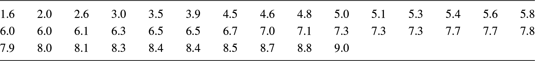
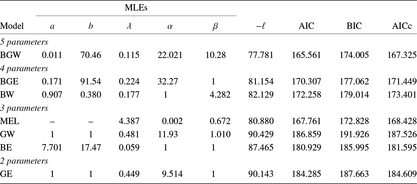
Table 4. MLEs of the parameters for the models fitted to the failure times data and the values of  $ -\ell $, AIC, BIC, and AICc.
4.1. Failure times of turbochargers
The first data set is given by Xu et al. [Reference Xu, Xie, Tang and Ho42] on the time to failure (103 h) of the turbocharger of one type of engine. Table 3 gives the measurements of the data set. Table 4 lists the MLEs of the parameters and the values of the goodness-of-fit statistics for the fitted models to the current data set.
From Table 3, we infer that the top two models for the first data set are the new three-parameter MEL and the five-parameter BGW distributions. However, the former has two fewer parameters to estimate and is, therefore, easier to use with less risk of overfitting. The TTT plot for failure times data presented in Figure 3(a) indicates an increasing hazard rate function. From Table 3, note that  $ \widehat{\alpha} \lt1 $ for the MEL model, which implies that the hazard rate function of this distribution is increasing, which is in accordance with Figure 3(a). The histogram of the data set with the plots of the estimated p.d.f.s of all fitted distributions are shown in Figure 3(b). This figure also depicts that the MEL and BGW distributions produce a better fit to the data set. Figure 3(c) shows the P–P plot for the MEL distribution and Figure 3(d) displays the empirical c.d.f. and estimated c.d.f. of the MEL distribution. From these figures, we also conclude that the proposed model is closely fitted to the failure times data.

Figure 3. Failure times data: (a) TTT plot; (b) histogram and p.d.f.s of the fitted models; (c) P–P plot of MEL model; and (d) empirical c.d.f. and estimated MEL c.d.f.
The estimated variance–covariance matrix  $ \bf{J}_{n}^{-1}(\widehat{\bf{\theta}}) $ of the MLEs under the MEL $(\alpha,\beta,\lambda)$ distribution for the current data are given by
 \begin{equation*}\bf{J}_{n}^{-1}(\widehat{\alpha}, \widehat{\beta}, \widehat{\lambda})=\left(\begin{array}{ccc}
1.35\times 10^{-7} & -4.09\times 10^{-6} & -0.00010 \\
-4.09\times 10^{-6} & 0.00100 & -0.27173 \\
-0.00010 & -0.27173 & 8.19040 \\
\end{array}\right) \text {. }
\end{equation*}
\begin{equation*}\bf{J}_{n}^{-1}(\widehat{\alpha}, \widehat{\beta}, \widehat{\lambda})=\left(\begin{array}{ccc}
1.35\times 10^{-7} & -4.09\times 10^{-6} & -0.00010 \\
-4.09\times 10^{-6} & 0.00100 & -0.27173 \\
-0.00010 & -0.27173 & 8.19040 \\
\end{array}\right) \text {. }
\end{equation*} Therefore, the approximate 95% confidence intervals for  $\alpha,$ β, and λ are, respectively, $[0.0022561,0.0022567]$, $[0.6527,0.6921]$, and $[-11.67,20.44]$.
4.2. Survival times of COVID-19 patients
Table 5. Survival times of COVID-19 patients.

Table 6. MLEs of the parameters for the models fitted to COVID-19 data and the values of  $ -\ell $, AIC, BIC, and AICc.

The second real data set presented in Table 5 corresponds to the survival times (in days) of 53 COVID-19 patients from January to February 2020 in China [Reference Liu, Ahmad, Gemeay, Abdulrahman, Hafez and Khalil29]. The value of MLEs of the parameters and the goodness-of-fit statistics for the fitted models to the current data are given in Table 6.
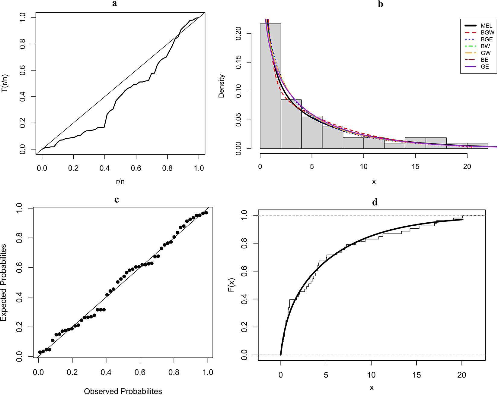
Figure 4. COVID-19 data: (a) TTT plot; (b) histogram and p.d.f.s of the fitted models; (c) P–P plot of MEL model; and (d) empirical c.d.f. and estimated MEL c.d.f.
Table 7. Life of fatigue fracture of Kevlar 373 epoxy.

Table 8. MLEs of the parameters for the models fitted to the fatigue life data and the values of  $ -\ell $, AIC, BIC, and AICc.

From this table, we can conclude that the MEL distribution presents the best performance when compared with the other fitted models to these data. We have  $ \widehat{\alpha} \gt 1 $ for the MEL model in Table 6, implying that the hazard rate function is decreasing. This fact is also in accordance with Figure 4(a). We provide the histogram of the data set with the plots of the estimated p.d.f.s in Figure 4(b), the P–P plot for the new model in Figure 4(c), and the empirical c.d.f. and estimated c.d.f. of the MEL distribution in Figure 4(d). These figures show that the new distribution fits these data adequately.
The estimated variance–covariance matrix  $ \bf{J}_{n}^{-1}(\widehat{\bf{\theta}}) $ of the MLEs under the MEL $(\alpha,\beta,\lambda)$ distribution for the current data are given by
 \begin{equation*}\bf{J}_{n}^{-1}(\widehat{\alpha}, \widehat{\beta}, \widehat{\lambda})=\left(\begin{array}{ccc}
3.24042 & 0.10985 & -0.08521 \\
0.10985 & 0.24189 & -0.08444 \\
-0.08521 & -0.08444 & 0.03143 \\
\end{array}\right) \text {. }
\end{equation*}
\begin{equation*}\bf{J}_{n}^{-1}(\widehat{\alpha}, \widehat{\beta}, \widehat{\lambda})=\left(\begin{array}{ccc}
3.24042 & 0.10985 & -0.08521 \\
0.10985 & 0.24189 & -0.08444 \\
-0.08521 & -0.08444 & 0.03143 \\
\end{array}\right) \text {. }
\end{equation*} Therefore, the approximate 95% confidence intervals for  $\alpha,$ β, and λ are, respectively, $[-2.72,9.98]$, $[0.1362,1.0844]$, and $[0.1974,0.3206]$.
4.3. Life of fatigue fracture of Kevlar 373 epoxy
The third data set reported by Andrews and Herzberg [Reference Andrews and Herzberg2] represents the life of fatigue fracture of Kevlar 373 epoxy that is subjected to constant pressure at the 90 stress level until all have failed. The measurements of this data set are presented in Table 7.
Table 8 and Figure 5(b) clearly prove the superiority of the new model over other competitive models for the current data. The TTT plot for the fatigue life data displayed in Figure 5(a) indicates increasing hazard rate function, which is confirmed by  $ \widehat{\alpha}$ for the MEL model in Table 8. Figure 5(c) and (d) also depict that the MEL distribution produces an adequate fit to the third data set.

Figure 5. Fatigue life data: (a) TTT plot; (b) histogram and p.d.f.s of the fitted models; (c) P–P plot of MEL model; and (d) empirical c.d.f. and estimated MEL c.d.f.
The estimated variance–covariance matrix  $ \bf{J}_{n}^{-1}(\widehat{\bf{\theta}}) $ of the MLEs under the MEL $(\alpha,\beta,\lambda)$ distribution for the current data are given by
 \begin{equation*}\bf{J}_{n}^{-1}(\widehat{\alpha}, \widehat{\beta}, \widehat{\lambda})=\left(\begin{array}{ccc}
0.00923 & -0.06351 & 0.00692 \\
-0.06351 & 0.23383 & -0.16097 \\
0.00692 & -0.16097 & 0.02502 \\
\end{array}\right) \text {. }
\end{equation*}
\begin{equation*}\bf{J}_{n}^{-1}(\widehat{\alpha}, \widehat{\beta}, \widehat{\lambda})=\left(\begin{array}{ccc}
0.00923 & -0.06351 & 0.00692 \\
-0.06351 & 0.23383 & -0.16097 \\
0.00692 & -0.16097 & 0.02502 \\
\end{array}\right) \text {. }
\end{equation*} Thus, the approximate 95% confidence intervals for  $\alpha,$ β, and λ are, respectively, $[-0.0067,0.3700]$, $[0.3520,4.5121]$, and $[-0.0096,0.6103]$.
5. Conclusion
In this paper, we have proposed a new three-parameter distribution, so-called the MEL distribution, by using the maximum entropy principle subject to the constraints on the mean and a GI. This GI is widely used for measuring concentration, variability, and uncertainty. The proposed MEL model has two shape parameters and one scale parameter. It includes exponential distribution as a special sub-model. The MEL p.d.f. can take various forms depending on its shape parameters. The new model can present both increasing and decreasing hazard rate functions. We have provided some of the mathematical properties of the new distribution, including quantiles, moments, mrl, characterization, and stochastic ordering. The model parameters are estimated using the maximum likelihood approach. The simulation results show that the method of maximum likelihood performs well in estimating the model parameters. Finally, three real data sets are analyzed to illustrate the importance and flexibility of the new proposed distribution in modeling lifetime data. In conclusion, the MEL distribution may provide a flexible mechanism for fitting a wide spectrum of positive real-world data sets. We hope the proposed model might serve as an alternative model to other models available in the literature for modeling real data in areas such as engineering, survival analysis, economics, and so on.
Acknowledgments
The authors thank the editor and anonymous reviewers for their insightful suggestions and positive remarks, which have considerably improved this paper.
Competing Interest
The authors declare no conflict of interest.
Appendix A. Appendix
A.1. Solution of the Bernoulli equation
The substitution  $ y=\bar{F}^{1-\gamma}$ reduces the Bernoulli Eq. (6) to the linear differential equation
 \begin{align}
\frac{{d}y}{{d}x}=c_1y+c_2.
\end{align}
\begin{align}
\frac{{d}y}{{d}x}=c_1y+c_2.
\end{align} By considering the boundary condition  $ y(0)=1 $, the solution of differential equation (A.1) is given by
 \begin{align*}
y(x)=\frac{c_1+c_2}{c_1}\ \mathrm{e}^{c_1x}-\frac{c_2}{c_1}.
\end{align*}
\begin{align*}
y(x)=\frac{c_1+c_2}{c_1}\ \mathrm{e}^{c_1x}-\frac{c_2}{c_1}.
\end{align*} Putting  $ \alpha=\frac{c_1+c_2}{c_1} $ and $\beta=c_1 $, we arrive at Eq. (7).
A.2. The BGW family
Singla et al. [Reference Singla, Jain and Sharma38] introduced a flexible five-parameter model called BGW distribution by considering the baseline distribution of beta generalized distribution [Reference Singh, Lee and George39] to be EW. The c.d.f. and p.d.f. of BGW distribution, respectively, are given by
 \begin{align*}
F(x)=\frac{1}{B(a, b)} \int_0^{\left(1-{\mathrm{e}}^{-(\lambda x)^\beta}\right)^\alpha} w^{a-1}(1-w)^{b-1}\mathrm{d}w,\quad x \gt 0
\end{align*}
\begin{align*}
F(x)=\frac{1}{B(a, b)} \int_0^{\left(1-{\mathrm{e}}^{-(\lambda x)^\beta}\right)^\alpha} w^{a-1}(1-w)^{b-1}\mathrm{d}w,\quad x \gt 0
\end{align*}and
 \begin{align*}
f(x)=\frac{\alpha \beta \lambda^{\beta} x^{\beta-1}}{B(a, b)}\left(1-{\mathrm{e}}^{-(\lambda x)^{\beta}}\right)^{\alpha a-1}\left\{1-\left(1-{\mathrm{e}}^{-(\lambda x)^{\beta}}\right)^{\alpha}\right\}^{b-1} {\mathrm{e}}^{-(\lambda x)^{\beta}}, \quad x \gt 0,
\end{align*}
\begin{align*}
f(x)=\frac{\alpha \beta \lambda^{\beta} x^{\beta-1}}{B(a, b)}\left(1-{\mathrm{e}}^{-(\lambda x)^{\beta}}\right)^{\alpha a-1}\left\{1-\left(1-{\mathrm{e}}^{-(\lambda x)^{\beta}}\right)^{\alpha}\right\}^{b-1} {\mathrm{e}}^{-(\lambda x)^{\beta}}, \quad x \gt 0,
\end{align*} where  $ B(a, b) $ is the beta function, λ > 0 is a scale parameter and $ a, b, \alpha, \beta \gt 0 $ are shape parameters. This distribution exhibits increasing, decreasing, bathtub, and upside-down bathtub-shaped failure rate functions for different parametric combinations. Singla et al. [Reference Singla, Jain and Sharma38] expressed the p.d.f. and c.d.f. of BGW distribution as mixtures of EW distribution. The BGW distribution unifies many existing distributions as its sub-models with applications in modeling a wide spectrum of real data sets in reliability and engineering. The sub-models of BGW distribution are as follows:
1. For β = 1, we get the BGE distribution.
2. If $a=b=1$, then BGW distribution reduces to the GW distribution. If in addition β = 2, we obtain GR distribution.
3. BW distribution arises as a special case of BGW by taking α = 1.
4. Assuming
$a=b=\beta=1$, we get GE distribution.5. With
$\alpha=\beta=1$, BE distribution can be obtained.6. For
$a=b=\alpha=1$, we obtain the Weibull (W) distribution with parameters λ and β. If in addition β = 2, the BGW distribution becomes Rayleigh (R) distribution.


The above relationships are also depicted in pictorial form in Figure A1.

Figure A1. Sub-models of BGW.


 Open access