


Introduction
The development of an abdominal aortic aneurysm (AAA) is a remodeling process that is triggered both by the degradation and the synthesis of extracellular matrix proteins and leads to the formation of local dilatations, which eventually lead to the rupture of an aortic wall (Niestrawska et al., Reference Niestrawska, Regitnig, Viertler, Cohnert, Babu and Holzapfel2019; Sherifova & Holzapfel, Reference Sherifova and Holzapfel2019). The most important structural proteins of the extracellular matrix are collagen and elastin, and both play an important role in the mechanical properties of the aortic tissue (Holzapfel & Ogden, Reference Holzapfel and Ogden2018; Sherifova & Holzapfel, Reference Sherifova and Holzapfel2020). Elastin ensures elasticity at lower stretch, whereas collagen determines the tensile strength at higher stretch (Weisbecker et al., Reference Weisbecker, Viertler, Pierce and Holzapfel2013; Chow et al., Reference Chow, Turcotte, Lin and Zhang2014; Schriefl et al., Reference Schriefl, Schmidt, Balzani, Sommer and Holzapfel2015). Collagen, therefore, takes on a decisive role in preventing ruptures (Holzapfel, Reference Holzapfel2008; Asgari et al., Reference Asgari, Latifi, Giovanniello, Espinosa and Amabili2022).
While tissue remodeling takes place during the development of an aneurysm, collagen is influenced in terms of content, cross-links, and structure (Tsamis et al., Reference Tsamis, Krawiec and Vorp2013). Although numerous studies have devoted themselves to the analysis of collagen content in AAA, this remains controversial, as an increase (Menashi et al., Reference Menashi, Campa, Greenhalgh and Powell1987; Rizzo et al., Reference Rizzo, McCarthy, Dixit, Lilly, Shively, Flinn and Yao1989; Lindeman et al., Reference Lindeman, Ashcroft, Beenakker, van Es, Koekkoek, Prins, Tielemans, Abdul-Hussien, Bank and Oosterkamp2010), no change (Gandhi et al., Reference Gandhi, Irizarry, Cantor, Keller, Nackman, Halpern, Newman and Tilson1994), or a decrease (Carmo et al., Reference Carmo, Colombo, Bruno, Corsi, Roncoroni, Cuttin, Radice, Mussini and Settembrini2002) has been reported. On the contrary, there is an agreement that the number of cross-links in AAAs is increasing (Bode et al., Reference Bode, Soini, Melkko, Satta, Risteli and Risteli2000; Carmo et al., Reference Carmo, Colombo, Bruno, Corsi, Roncoroni, Cuttin, Radice, Mussini and Settembrini2002; Lindeman et al., Reference Lindeman, Ashcroft, Beenakker, van Es, Koekkoek, Prins, Tielemans, Abdul-Hussien, Bank and Oosterkamp2010). The structural changes observed include the loss of distinction between the layers (Gasser et al., Reference Gasser, Gallinetti, Xing, Forsell, Swedenborg and Roy2012; Niestrawska et al., Reference Niestrawska, Viertler, Regitnig, Cohnert, Sommer and Holzapfel2016, Reference Niestrawska, Regitnig, Viertler, Cohnert, Babu and Holzapfel2019), changes in the orientation and dispersion of collagen fibers (Gasser et al., Reference Gasser, Gallinetti, Xing, Forsell, Swedenborg and Roy2012; Niestrawska et al., Reference Niestrawska, Viertler, Regitnig, Cohnert, Sommer and Holzapfel2016, Reference Niestrawska, Regitnig, Viertler, Cohnert, Babu and Holzapfel2019), and the decrease in their waviness (Niestrawska et al., Reference Niestrawska, Viertler, Regitnig, Cohnert, Sommer and Holzapfel2016) and the increase in the diameter (Niestrawska et al., Reference Niestrawska, Viertler, Regitnig, Cohnert, Sommer and Holzapfel2016; Urabe et al., Reference Urabe, Hoshina, Shimanuki, Nishimori, Miyata and Deguchi2016). The available quantified structural data are limited to orientation and dispersion (Gasser et al., Reference Gasser, Gallinetti, Xing, Forsell, Swedenborg and Roy2012; Niestrawska et al., Reference Niestrawska, Viertler, Regitnig, Cohnert, Sommer and Holzapfel2016, Reference Niestrawska, Regitnig, Viertler, Cohnert, Babu and Holzapfel2019; Amabili et al., Reference Amabili, Asgari, Breslavsky, Franchini, Giovanniello and Holzapfel2021). To advance the understanding of structural changes caused by aneurysm development and to improve material (Holzapfel et al., Reference Holzapfel, Gasser and Ogden2000; Gasser et al., Reference Gasser, Ogden and Holzapfel2006; Holzapfel et al., Reference Holzapfel, Niestrawska, Ogden, Reinisch and Schriefl2015; Weisbecker et al., Reference Weisbecker, Unterberger and Holzapfel2015; Li et al., Reference Li, Ogden and Holzapfel2018; Franchini et al., Reference Franchini, Breslavsky, Giovanniello, Kassab, Holzapfel and Amabili2022) and multiscale (Hayenga et al., Reference Hayenga, Thorne, Peirce and Humphrey2011; Thunes et al., Reference Thunes, Phillippi, Gleason, Vorp and Maiti2018; Dalbosco et al., Reference Dalbosco, Carniel, Fancello and Holzapfel2021) modeling of the aortic tissues and the formation of aneurysms, this study provides the measured values for orientation and dispersion as well as for the first time the diameter and waviness of collagen fibers in human abdominal aortas.
In this article, we first give a brief overview of pathological changes in the arterial wall caused by AAA. In the absence of an established method for quantifying the diameter and waviness of collagen fibers in aortic tissues, we provide a background for methods currently used to quantify collagen fibers from other locations, vessels, and nerve fibers. Then we describe the algorithms that we developed for the aortic collagen. Finally, we evaluate and discuss the structural parameters, diameter, waviness, orientation, and dispersion that are measured in healthy and aneurysmal human abdominal aortas.
Background
Pathological Changes in Collagen from AAA
A healthy abdominal aorta consists of three clearly distinguishable layers, namely intima, media, and adventitia, which are all reinforced by collagen of mostly type I and III (Menashi et al., Reference Menashi, Campa, Greenhalgh and Powell1987; Rizzo et al., Reference Rizzo, McCarthy, Dixit, Lilly, Shively, Flinn and Yao1989; Bode et al., Reference Bode, Soini, Melkko, Satta, Risteli and Risteli2000; Holzapfel, Reference Holzapfel2008). In the case of an aneurysm, types I and III remain the main collagen types in the aortic wall (Menashi et al., Reference Menashi, Campa, Greenhalgh and Powell1987; Rizzo et al., Reference Rizzo, McCarthy, Dixit, Lilly, Shively, Flinn and Yao1989; Bode et al., Reference Bode, Soini, Melkko, Satta, Risteli and Risteli2000). In addition, the ratio of type I to type III for the intact wall remains unchanged (3:1), as reported by Rizzo et al. (Reference Rizzo, McCarthy, Dixit, Lilly, Shively, Flinn and Yao1989), as well as for the medial layer (2:1), as described by Menashi et al. (Reference Menashi, Campa, Greenhalgh and Powell1987). On the other hand, Bode et al. (Reference Bode, Soini, Melkko, Satta, Risteli and Risteli2000) detected newly synthesized type I collagen in the intima and type III in the media. Overall, the change in the collagen content in an aneurysm is still being discussed (Tsamis et al., Reference Tsamis, Krawiec and Vorp2013). An increased collagen content has been reported by Menashi et al. (Reference Menashi, Campa, Greenhalgh and Powell1987) and Rizzo et al. (Reference Rizzo, McCarthy, Dixit, Lilly, Shively, Flinn and Yao1989) and further supported by Lindeman et al. (Reference Lindeman, Ashcroft, Beenakker, van Es, Koekkoek, Prins, Tielemans, Abdul-Hussien, Bank and Oosterkamp2010). In contrast, Carmo et al. (Reference Carmo, Colombo, Bruno, Corsi, Roncoroni, Cuttin, Radice, Mussini and Settembrini2002) suggested a reduced collagen content, and Gandhi et al. (Reference Gandhi, Irizarry, Cantor, Keller, Nackman, Halpern, Newman and Tilson1994) did not detect any changes. Interestingly, an increase in cross-links is generally accepted (Bode et al., Reference Bode, Soini, Melkko, Satta, Risteli and Risteli2000; Carmo et al., Reference Carmo, Colombo, Bruno, Corsi, Roncoroni, Cuttin, Radice, Mussini and Settembrini2002; Lindeman et al., Reference Lindeman, Ashcroft, Beenakker, van Es, Koekkoek, Prins, Tielemans, Abdul-Hussien, Bank and Oosterkamp2010; Tsamis et al., Reference Tsamis, Krawiec and Vorp2013).
Healthy aortic layers show pronounced collagen structures. Viewed in a longitudinal–circumferential plane (in-plane), the intimal collagen shows a rather isotropic, carpet-like organization, followed by two counter-rotating fiber families in the media oriented in the circumferential direction and two longitudinally oriented fiber families in the adventitia (Schriefl et al., Reference Schriefl, Zeindlinger, Pierce, Regitnig and Holzapfel2012b, Reference Schriefl, Wolinski, Regitnig, Kohlwein and Holzapfel2013; Niestrawska et al., Reference Niestrawska, Viertler, Regitnig, Cohnert, Sommer and Holzapfel2016; Amabili et al., Reference Amabili, Asgari, Breslavsky, Franchini, Giovanniello and Holzapfel2021). A view from a radial–circumferential plane (out-of-plane) shows almost circumferentially oriented fibers without radial components and very little dispersion through the wall thickness (Schriefl et al., Reference Schriefl, Zeindlinger, Pierce, Regitnig and Holzapfel2012b, Reference Schriefl, Wolinski, Regitnig, Kohlwein and Holzapfel2013; Niestrawska et al., Reference Niestrawska, Viertler, Regitnig, Cohnert, Sommer and Holzapfel2016; Amabili et al., Reference Amabili, Asgari, Breslavsky, Franchini, Giovanniello and Holzapfel2021). The aneurysm development influences the structure (and mechanics) of the collagen fibers (Tsamis et al., Reference Tsamis, Krawiec and Vorp2013). Lindeman et al. (Reference Lindeman, Ashcroft, Beenakker, van Es, Koekkoek, Prins, Tielemans, Abdul-Hussien, Bank and Oosterkamp2010) reported on a remodeled collagen architecture that no longer behaves like a coherent network. This study with atomic force microscopy cantilevers showed that mechanical forces acting on individual fibers in AAA were no longer distributed over an adventitial tissue.
Niestrawska et al. (Reference Niestrawska, Regitnig, Viertler, Cohnert, Babu and Holzapfel2019) carried out biaxial extension tests on aneurysmal tissues and assigned changes in the orientation and dispersion of collagen fibers to changes in the mechanics. A reorientation of the intimal and adventitial collagen has been suggested as the reason for the loss of initial stiffness. Subsequently, isotropically distributed collagen on the abluminal side led to increased compliance. After all, the increased isotropy was associated with rapid stiffening. Previously, Gasser et al. (Reference Gasser, Gallinetti, Xing, Forsell, Swedenborg and Roy2012) and Niestrawska et al. (Reference Niestrawska, Viertler, Regitnig, Cohnert, Sommer and Holzapfel2016) found a loss of the characteristic layer structure, measured the orientation and dispersion of collagen fibers, and reported a higher fiber dispersion out-of-plane in aneurysmal aortic walls. Neither the waviness nor the diameter of the collagen fibers have been quantified so far. Niestrawska et al. (Reference Niestrawska, Viertler, Regitnig, Cohnert, Sommer and Holzapfel2016) and Urabe et al. (Reference Urabe, Hoshina, Shimanuki, Nishimori, Miyata and Deguchi2016) pointed to thicker collagen struts in aneurysmal tissues compared to healthy tissue, while Niestrawska et al. (Reference Niestrawska, Viertler, Regitnig, Cohnert, Sommer and Holzapfel2016) also documented that the collagen fibers in the abluminal layer of AAAs have lost their waviness.
Quantification of the Fiber Diameter
The diameter of tubular structures, such as fibers or vessels, is assumed to be equal to the thickness of the fiber (or vessel) represented by a projection parallel to its centerline (Pickering et al., Reference Pickering, Ford and Chow1996; Brightman et al., Reference Brightman, Rajwa, Sturgis, McCallister, Robinson and Voytik-Harbin2000; Heneghan et al., Reference Heneghan, Flynn, O'Keefe and Cahill2002; Roeder et al., Reference Roeder, Kokini, Sturgis, Robinson and Voytik-Harbin2002; Wu et al., Reference Wu, Rajwa, Filmer, Hoffmann, Yuan, Chiang, Sturgis and Robinson2003; Ziabari et al., Reference Ziabari, Mottaghitalab and Haghi2009; D'Amore et al., Reference D'Amore, Stella, Wagner and Sacks2010; Mencucci et al., Reference Mencucci, Marini, Paladini, Sarchielli, Sgambati, Menchini and Vannelli2010; Changoor et al., Reference Changoor, Nelea, Méthot, Tran-Khanh, Chevrier, Restrepo, Shive, Hoemann and Buschmann2011; Chen et al., Reference Chen, Liu, Slipchenko, Zhao, Cheng and Kassab2011, Reference Chen, Slipchenko, Liu, Zhao, Cheng, Lanir and Kassab2013; Koch et al., Reference Koch, Tsamis, D'Amore, Wagner, Watkins, Gleason and Vorp2014). The perpendicular projection is an alternative; in this case, the diameter of the fiber (or vessel) is the diameter of the projected circle (Almutairi et al., Reference Almutairi, Cootes and Kadler2015). While the definition is simple, there are several factors that affect the measurement such as the quality of the microscopy images, the angular deviation between the projection plane and the centerline, and the wavy character of the observed structures. The aspects mentioned above could explain the difficulties in establishing automated procedures. However, the usual manual approach to measuring the diameter is supported by image analysis software (Pickering et al., Reference Pickering, Ford and Chow1996; Brightman et al., Reference Brightman, Rajwa, Sturgis, McCallister, Robinson and Voytik-Harbin2000; Roeder et al., Reference Roeder, Kokini, Sturgis, Robinson and Voytik-Harbin2002; Mencucci et al., Reference Mencucci, Marini, Paladini, Sarchielli, Sgambati, Menchini and Vannelli2010; Changoor et al., Reference Changoor, Nelea, Méthot, Tran-Khanh, Chevrier, Restrepo, Shive, Hoemann and Buschmann2011; Chen et al., Reference Chen, Liu, Slipchenko, Zhao, Cheng and Kassab2011, Reference Chen, Slipchenko, Liu, Zhao, Cheng, Lanir and Kassab2013). With manual measurement, the operator typically selects two points that define the fiber diameter (i.e. thickness in projection parallel to the centerline of the fiber), measures the distance between these points in pixels, and converts it to micrometers based on the pixel size. Similar techniques have been chosen to assess the diameter of collagen fibers by, for example, Pickering et al. (Reference Pickering, Ford and Chow1996) in human coronary atherosclerotic lesions, Mencucci et al. (Reference Mencucci, Marini, Paladini, Sarchielli, Sgambati, Menchini and Vannelli2010) in the human cornea, Changoor et al. (Reference Changoor, Nelea, Méthot, Tran-Khanh, Chevrier, Restrepo, Shive, Hoemann and Buschmann2011) in human articular cartilage, or Chen et al. (Reference Chen, Liu, Slipchenko, Zhao, Cheng and Kassab2011, Reference Chen, Slipchenko, Liu, Zhao, Cheng, Lanir and Kassab2013) in porcine coronary arteries. Similarly, Brightman et al. (Reference Brightman, Rajwa, Sturgis, McCallister, Robinson and Voytik-Harbin2000) and Roeder et al. (Reference Roeder, Kokini, Sturgis, Robinson and Voytik-Harbin2002) assessed collagen scaffolds using images with binarized fibers.
For retinal vessels (Heneghan et al., Reference Heneghan, Flynn, O'Keefe and Cahill2002), collagenous scaffolds (Wu et al., Reference Wu, Rajwa, Filmer, Hoffmann, Yuan, Chiang, Sturgis and Robinson2003; Ziabari et al., Reference Ziabari, Mottaghitalab and Haghi2009), or soft tissues (D'Amore et al., Reference D'Amore, Stella, Wagner and Sacks2010; Koch et al., Reference Koch, Tsamis, D'Amore, Wagner, Watkins, Gleason and Vorp2014), algorithms have been developed that allow diameter measurements in binary images. Heneghan et al. (Reference Heneghan, Flynn, O'Keefe and Cahill2002) suggested defining a point in a binarized vessel and drawing line segments that pass through this point for all possible rotations, while all segments were contained within the binarized vessel. The smallest segment was taken as the vessel diameter. Wu et al. (Reference Wu, Rajwa, Filmer, Hoffmann, Yuan, Chiang, Sturgis and Robinson2003) determined the diameter of fibers in collagen matrices with the help of the Euclidean distance transform (Borgefors, Reference Borgefors1986). Ziabari et al. (Reference Ziabari, Mottaghitalab and Haghi2009) proposed a replacement for the distance transform to study the diameter of electrospun nanofibers. The proposed method comprises drawing a horizontal segment within a fiber, finding the center of that segment, and drawing a vertical segment from that center to the edge of the fiber. The fiber diameter is then calculated based on these segments. Although the authors concluded that their method gave more accurate results, it is worth noting that electrospun nanofibers are straight and this algorithm has not been validated for wavy fibers. D'Amore et al. (Reference D'Amore, Stella, Wagner and Sacks2010) combined binarized centerlines with grayscale images to analyze rat collagen scaffolds and carotid arteries. The binarized centerlines were used to select a portion of a fiber between the network nodes. Gray intensity and gray intensity gradient of grayscale images were used to extract a fiber from the background or from a bundle. Koch et al. (Reference Koch, Tsamis, D'Amore, Wagner, Watkins, Gleason and Vorp2014) chose distance transform again to measure the diameter of fibers in the human thoracic aortas. Unfortunately, the results obtained were only shown in pixels, so the data cannot be used as a quantitative reference. Nevertheless, the distance transform for our study (see the section “Diameter” for more details) was chosen as a stable and sufficiently fast solution.
Quantification of Fiber Waviness
Numerous metrics of waviness, also known as tortuosity, are proposed in the literature (Dougherty & Varro, Reference Dougherty and Varro2000; Bullitt et al., Reference Bullitt, Gerig, Pizer, Lin and Aylward2003; Grisan et al., Reference Grisan, Foracchia and Ruggeri2008; Koprowski et al., Reference Koprowski, Teper, Wȩglarz, Wylȩgała, Krejca and Wróbel2012; Ghazanfari et al., Reference Ghazanfari, Driessen-Mol, Sanders, Dijkman, Hoerstrup, Baaijens and Bouten2015; Annunziata et al., Reference Annunziata, Kheirkhah, Aggarwal, Hamrah and Trucco2016). Bullitt et al. (Reference Bullitt, Gerig, Pizer, Lin and Aylward2003) has listed and compared three of them, namely the distance metric, the inflection count metric, and the sum of angles metric. The distance metric provides a relationship between the actual length of a curve and the linear distance between its end-points. Although commonly used (Heneghan et al., Reference Heneghan, Flynn, O'Keefe and Cahill2002; Rezakhaniha et al., Reference Rezakhaniha, Agianniotis, Schrauwen, Griffa, Sage, Bouten, van de Vosse, Unser and Stergiopulos2012; Fata et al., Reference Fata, Carruthers, Gibson, Watkins, Gottlieb, Mayer and Sacks2013; Chow et al., Reference Chow, Turcotte, Lin and Zhang2014; Koch et al., Reference Koch, Tsamis, D'Amore, Wagner, Watkins, Gleason and Vorp2014; Zeinali-Davarani et al., Reference Zeinali-Davarani, Wang, Chow, Turcotte and Zhang2015), this measure has a significant disadvantage, since it shows the same value for a fiber with a high amplitude and only one inflection point as for a fiber with a low amplitude, but several inflection points. The inflection count metric overcomes this disadvantage by multiplying a value of the distance metric by a number of inflection points. The sum of angles metric is an alternative approach in which the total curvature is integrated along a curve and normalized by the curve length. The latter approach is particularly useful with a three-dimensional helical curve. It has been shown that this metric is able to distinguish between three helices of the same length but variable frequency and amplitude, while neither the distance metric nor the inflection count metric was able to identify their different tortuosities. The distance metric was unsuccessful because of identical lengths and the inflection count metric because of missing inflection points on a helical curve. In contrast, the sum of angles metric performed poorly on a set of three sinusoidal waves with the same frequency but different amplitude, while both the distance metric and the inflection count metric gave satisfactory results, see Bullitt et al. (Reference Bullitt, Gerig, Pizer, Lin and Aylward2003).
Grisan et al. (Reference Grisan, Foracchia and Ruggeri2008) proposed a measure based on dividing the curve into segments at inflection points, calculating the distance metric for each segment, and finally summarizing all the metrics and their number. This measure was specially developed for retinal vessels and goes well with clinically perceived tortuosity. For large vessels, such as an aorta, Dougherty & Varro (Reference Dougherty and Varro2000) proposed a measurement based on second differences in the coordinates of the vessel centerline, since the distance metric was not sensitive enough for this application. Koprowski et al. (Reference Koprowski, Teper, Wȩglarz, Wylȩgała, Krejca and Wróbel2012) reduced the tortuosity problem to an inclination angle for eye fundus vessels. The Gabor wavelet method (Arivazhagan et al., Reference Arivazhagan, Ganesan and Priyal2006) was used by Ghazanfari et al. (Reference Ghazanfari, Driessen-Mol, Sanders, Dijkman, Hoerstrup, Baaijens and Bouten2015) for the quantification of collagen fibers in sheep explants of tissue-engineered heart valves. A tortuosity index was calculated as one minus the maximum number in the Gabor histogram, which was the histogram of Gabor wavelets with different angles of orientation and wavelengths. However, the detection of fiber tortuosity was limited to images of fibers with a defined orientation and was unsuccessful with randomly distributed fibers. An alternative approach was proposed by Annunziata et al. (Reference Annunziata, Kheirkhah, Aggarwal, Hamrah and Trucco2016) for the analysis of corneal nerve fibers. The proposed concept was called definition-free and included multirange context filters in which discriminative multiscale features were learned for specific anatomical objects and diseases. Although promising, this method requires application-specific images with predefined tortuosity at various scales in order to train a regressor.
In summary, it can be said that no single tortuosity metric is able to cope with all applications, since tortuosity has a different character for different anatomical and biological structures. Most advanced techniques require the skeletonization of images to extract centerlines from fibers (Dougherty & Varro, Reference Dougherty and Varro2000; Bullitt et al., Reference Bullitt, Gerig, Pizer, Lin and Aylward2003; Grisan et al., Reference Grisan, Foracchia and Ruggeri2008; Annunziata et al., Reference Annunziata, Kheirkhah, Aggarwal, Hamrah and Trucco2016). The skeletonization of collagen fibers in microscopic images is very demanding, among other things because of the crossing and overlapping fibers. Therefore, manual fiber tracking and the distance metric have been routinely used to assess collagen waviness in vascular tissues, that is, rabbit common carotid arteries (Rezakhaniha et al., Reference Rezakhaniha, Agianniotis, Schrauwen, Griffa, Sage, Bouten, van de Vosse, Unser and Stergiopulos2012), ovine main pulmonary arteries (Fata et al., Reference Fata, Carruthers, Gibson, Watkins, Gottlieb, Mayer and Sacks2013), and porcine thoracic aortas (Chow et al., Reference Chow, Turcotte, Lin and Zhang2014; Zeinali-Davarani et al., Reference Zeinali-Davarani, Wang, Chow, Turcotte and Zhang2015). The tracing and the measurements were usually supported by the plug-in NeuronJ (Meijering et al., Reference Meijering, Jacob, Sarria, Steiner, Hirling and Unser2004) from the software ImageJ (Schindelin et al., Reference Schindelin, Arganda-Carreras, Frise, Kaynig, Longair, Pietzsch, Preibisch, Rueden, Saalfeld, Schmid, Tinevez, White, Hartenstein, Eliceiri, Tomancak and Cardona2012), as in Rezakhaniha et al. (Reference Rezakhaniha, Agianniotis, Schrauwen, Griffa, Sage, Bouten, van de Vosse, Unser and Stergiopulos2012), Chow et al. (Reference Chow, Turcotte, Lin and Zhang2014), and Zeinali-Davarani et al. (Reference Zeinali-Davarani, Wang, Chow, Turcotte and Zhang2015). Although it was successful in locating the adventitial collagen bundles, the manual method failed in locating the medial collagen fibers (Chow et al., Reference Chow, Turcotte, Lin and Zhang2014). Chow et al. (Reference Chow, Turcotte, Lin and Zhang2014), therefore, suggested using the fractal analysis as a measure of the fiber waviness. In addition, Koch et al. (Reference Koch, Tsamis, D'Amore, Wagner, Watkins, Gleason and Vorp2014) proposed an algorithm for automating fiber quantification that involves the segmentation and skeletonization of collagen fibers from the human thoracic aorta. Although it was tested with out-of-plane images of the arterial wall and in-plane images of the adventitia, it did not prove successful with in-plane medial images. To overcome the above limitations, here we recommend tracking just a single wave of collagen fiber and measuring the amplitude and tortuosity with the distance metric (for more details, see the section “Waviness”).
Methods
Sample Preparation
Twelve samples of healthy abdominal aortas with non-atherosclerotic intimal thickening (59 ± 7 years old, six females and six males) were collected within 24 h after death (Institute of Pathology, Medical University Graz, Graz, Austria) and stored in 0.9% physiological saline solution at 4°C until imaging. The samples used are those documented in Niestrawska et al. (Reference Niestrawska, Viertler, Regitnig, Cohnert, Sommer and Holzapfel2016). Ten samples of aneurysmal abdominal aortas (67 ± 7 years old, two females and eight males) were collected during open aneurysm repair (Department of Vascular Surgery, Medical University Graz, Graz, Austria) and stored in Dulbecco's modified Eagle's medium (to preserve a possible thrombus) at 4°C until imaging. The aneurysmal abdominal aortic samples used are those documented in Niestrawska et al. (Reference Niestrawska, Regitnig, Viertler, Cohnert, Babu and Holzapfel2019). A rectangular piece approximately 15 × 5 mm was cut from each sample, with the longer edge marking the longitudinal direction of the aorta.
Second-Harmonic Generation Microscopic Imaging
Before recording, all specimens were optically cleared according to Schriefl et al. (Reference Schriefl, Wolinski, Regitnig, Kohlwein and Holzapfel2013). First, each specimen was dehydrated with a graded ethanol series. Next, the specimens were immersed in a 1:2 solution of ethanol:benzyl alcohol–benzyl benzoate (BABB) for 4 h and then stored in 100% BABB for at least 12 h. All steps were carried out at room temperature.
Second-harmonic generation (SHG) microscopy imaging was carried out at the Institute of Science and Technology in Klosterneuburg, Austria, using a setup consisting of a Chameleon Titan Saphir laser (Coherent, Inc., USA) integrated into a TriM Scope II confocal microscope (LaVision BioTec GmbH, Germany). The SHG signal was induced by a laser tuned to 880 nm, and the emitted signal was transmitted from a BP 460/50 emission filter to a detector. A Leica IMM CORR CS2 20× water immersion objective was used to take images of 1024 × 1024 pixels, with a pixel size of 0.5 × 0.5 μm in z-stacks of 5 μm steps.
Quantification of Collagen Fibers
Diameter
The SHG images of the media showed clearly distinguishable fibers, whereas fiber bundles were observed in the adventitia. Following Lindeman et al. (Reference Lindeman, Ashcroft, Beenakker, van Es, Koekkoek, Prins, Tielemans, Abdul-Hussien, Bank and Oosterkamp2010), we considered the bundle to be mechanically representative. Thus, the bundle diameter was measured in the healthy adventitia and, if it was pronounced, in the aneurysmal tissue. Otherwise, the fiber diameter was measured as for the healthy media. Since the captured SHG images show fibers and bundles parallel to their centerlines, the diameter of both fibers and bundles was recognized from their thickness, as shown in Figure 1. A script was written with MATLAB commands (The MathWorks Inc., 2021) to efficiently measure the diameter of a single fiber or a bundle of fibers. First, a region of interest was selected for processing because the signal-to-noise ratio varied widely within the image. The following procedure consists of two main parts: image processing, which leads to binarization, and diameter detection of the binary images.

Fig. 1. Representative region of an SHG image showing medial (M) and adventitial (A) collagen of a healthy abdominal aorta. On exemplary medial collagen fibers and adventitial collagen bundles, the thickness, which resembles the diameter, is marked.
The image processing begins with the contrast increase through intensity adjustment (MATLAB function: imadjust) and then with the removal of the impulse noise (medfilt2). The contrast is then enhanced by histogram equalization (histeq), as described in a similar way by D'Amore et al. (Reference D'Amore, Stella, Wagner and Sacks2010) and Koch et al. (Reference Koch, Tsamis, D'Amore, Wagner, Watkins, Gleason and Vorp2014). The further image processing consists of two pipelines developed for fibers and bundles. A flowchart of the image processing workflow is shown in Figure 2.

Fig. 2. SHG image processing flowchart: steps that apply to both fibers and bundles are drawn with solid lines, whereas dashed lines indicate additional steps that pertain to fiber processing.
The preprocessed grayscale image is converted into a binary image (imbinarize) whereby the threshold value for the bundles was calculated using the Otsu method (global) and a locally adaptive threshold is used for the fibers (adaptive). The structuring element, a disc with a pixel radius, is used to remove objects (imopen) and to fill holes (imclose) that are smaller than the structuring element. The edge detection (edge) is an additional step that is carried out on a grayscale image for fiber processing. The recognized edges are then subtracted from the segmented image. The grayscale image is processed again to obtain regional maxima (imextendedmax) that are used as a mask for the segmented image. The mask is applied to identify the brightest objects, that is, objects with the strongest recorded signal.
The diameter of the object of the binary image is recognized by means of the Euclidean distance transform (Borgefors, Reference Borgefors1986), see Wu et al. (Reference Wu, Rajwa, Filmer, Hoffmann, Yuan, Chiang, Sturgis and Robinson2003) and Koch et al. (Reference Koch, Tsamis, D'Amore, Wagner, Watkins, Gleason and Vorp2014). The main disadvantage of the distance transform method is the permanent error of one pixel when the width is an even number. Since the object represents the fiber, the diameter of a fiber is measured as the diameter of the circle inscribed on the fiber, similar to that described by Wu et al. (Reference Wu, Rajwa, Filmer, Hoffmann, Yuan, Chiang, Sturgis and Robinson2003). The circle is defined by the pixel with the maximum value of the distance transform; therefore, the position of the pixel is the position of the center of the circle and the radius is equal to this value. Finally, the operator is shown the grayscale image with inscribed circles, as shown in Figure 3, for confirmation or, alternatively, for rejection.
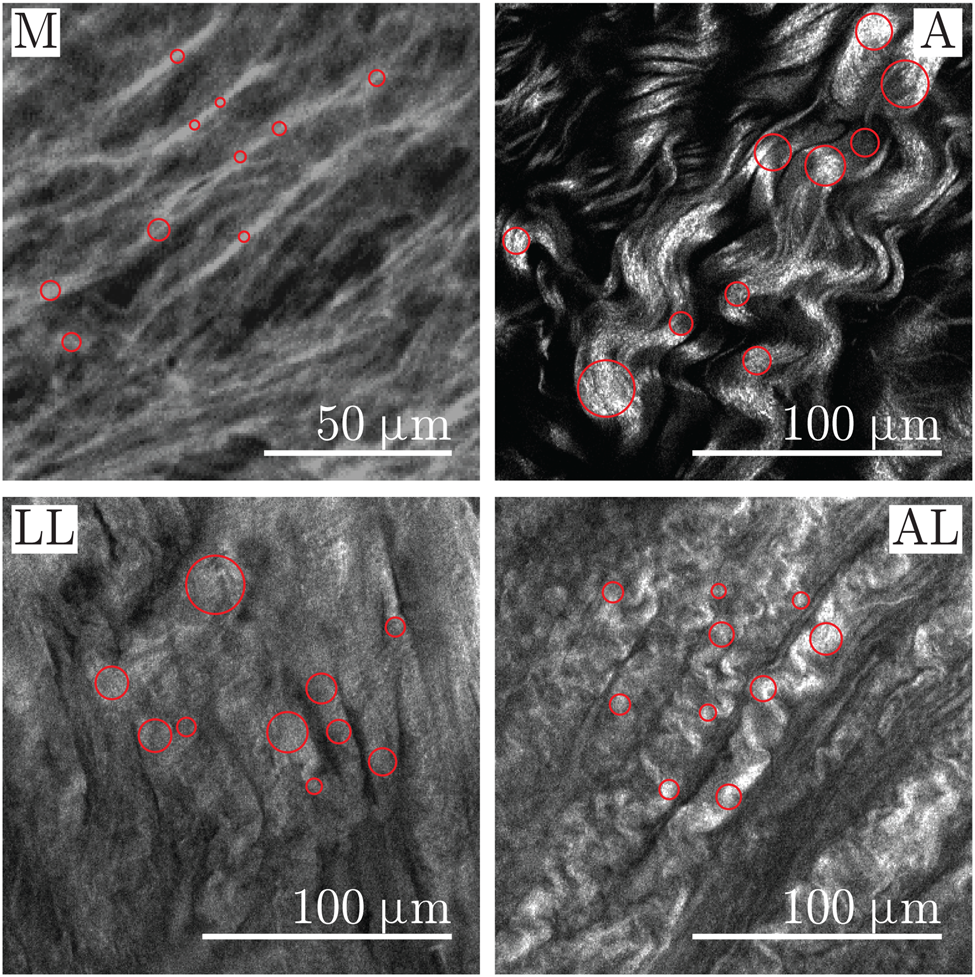
Fig. 3. Close-ups of representative SHG images showing the media (M) and adventitia (A) of healthy aortas as well as the luminal layer (LL) and the abluminal layer (AL) of AAAs. The measurement points of the diameter are visualized as circles in collagen fibers on the media and in bundles of collagen fibers on the adventitia and on the LL and AL of AAA.
The algorithm for image processing and segmentation was validated on sine-wave grating images and on SHG images. As described by Semmlow (Reference Semmlow2004), the sine-wave grating images were generated with different image sizes, different amplitudes, and number of grating cycles. The images were processed as previously described, after which the boundary of the segmented image (MATLAB function: bwboundaries) was marked on the original sine-wave grating image. The same procedure was applied on all healthy media images and five sets of healthy adventitia. A human operator was involved in judging the boundary recognition, and the boundary recognition was judged to be satisfactory. The diameter detection algorithm was tested on binary images. The rectangular and sine-wave objects of known size and width were generated with MATLAB (The MathWorks Inc., 2021). The detected diameter was, as expected based on the distance transform method used, within one pixel error.
Waviness
The most common definition of tortuosity, as described in the section “Quantification of Fiber Waviness,” assumes that an entire collagen fiber is visible from one end to the other in an image. However, we could not clearly distinguish the beginning and end of single fibers as they may not be in the same image. We, therefore, ask when studies on aortic collagen tortuosity identified the respective beginning and end in SHG images. Note that tortuosity does not distinguish between a high-amplitude fiber and only one inflection point and a low-amplitude fiber but multiple inflection points, as we explained in detail in the section “Quantification of Fiber Waviness.”
Therefore, we define tortuosity using a single wave of collagen fiber, as shown in Figure 4 (Towler, Reference Towler2017), and calculate tortuosity T as
 $$T = L_{\,f}/L_0,\; $$
where L 0 denotes the end-point-distance and Lf the arc length, similar to the study by, for example, Heneghan et al. (Reference Heneghan, Flynn, O'Keefe and Cahill2002). The higher the value of T the more wavy the measured fiber. In addition, we calculated a straightness parameter S as
 $$S = 1/T,$$
to match the results obtained with the findings of Rezakhaniha et al. (Reference Rezakhaniha, Agianniotis, Schrauwen, Griffa, Sage, Bouten, van de Vosse, Unser and Stergiopulos2012).

Fig. 4. Representative region of a SHG image showing adventitial collagen from a healthy abdominal aorta. Definitions for the peak-to-peak amplitude A (green dotted line), the end-point-distance L 0 (blue solid line), and the arc length Lf (red curve) are shown for a single wave measured from peak to peak.
Tortuosity alone is not enough to characterize the waviness of a fiber, since fibers with large amplitudes and small end-point-distances can have values similar to fibers with small amplitudes and larger end-point distances. Therefore, we also measured the peak-to-peak amplitude A of a single wave of a collagen fiber, as shown in Figure 4. The software ImageJ (Schindelin et al., Reference Schindelin, Arganda-Carreras, Frise, Kaynig, Longair, Pietzsch, Preibisch, Rueden, Saalfeld, Schmid, Tinevez, White, Hartenstein, Eliceiri, Tomancak and Cardona2012) with the plugin NeuronJ (Meijering et al., Reference Meijering, Jacob, Sarria, Steiner, Hirling and Unser2004) was used and combined with MATLAB (The MathWorks Inc., 2021). Here, NeuronJ was used to track the individual waves of collagen fibers or bundles. Representative examples of tracking different layers can be found in Figure 5. A custom-made MATLAB script used the curves from NeuronJ and calculated both the amplitudes A and the tortuosities T. Note that straight fibers do not have clear end-points. As a result, the end-point distance of straight fibers cannot be clearly defined and compared with the end-point distance of wavy fibers. The tortuosity measurement is not influenced, however, since both Lf and L 0 have the same value in straight fibers.

Fig. 5. Representative SHG images showing the tracing in red. Tracing performed on the media (M) and adventitia (A) of healthy aortas as well as the LL and the AL of AAAs. Note that the structure of the AAA layers varied from sample to sample.
Orientation and Dispersion
The orientation and dispersion of collagen fibers were analyzed according to Schriefl et al. (Reference Schriefl, Reinisch, Sankaran, Pierce and Holzapfel2012a, Reference Schriefl, Wolinski, Regitnig, Kohlwein and Holzapfel2013), Niestrawska et al. (Reference Niestrawska, Viertler, Regitnig, Cohnert, Sommer and Holzapfel2016), and Holzapfel et al. (Reference Holzapfel, Niestrawska, Ogden, Reinisch and Schriefl2015). Briefly, a combination of Fourier power spectrum analysis and wedge filtering was used to obtain discrete angular distributions with a resolution of 1° relative intensities corresponding to the fiber orientation. The fiber orientations obtained were fitted to the von Mises distribution for the probability density by means of the maximum likelihood estimation, independently for in-plane (ρ ip) and out-of-plane (ρ op), that is,
 $$\eqalign{\rho_{\rm ip}( \mathit{\Phi}) &= {\exp[ a\cos 2( \mathit{\Phi}\pm\alpha) ] \over I_{0}( a) },\; \cr \rho_{\rm op}( \mathit{\Theta}) &= 2 \sqrt{{2b\over \pi}} {\exp[ b( \cos 2\mathit{\Theta}-1) ] \over {\rm erf}( \sqrt{2b}) },\;} $$
where  $\mathit {\Phi }\in [ 0,\; 2\pi ]$ and $\mathit {\Theta }\in [ -\pi /2,\; \pi /2]$ represent the general in-plane and out-of-plane fiber directions, respectively, α is the mean in-plane fiber direction, a and b are concentration parameters, and I 0(a) is the modified Bessel function of the first kind of order 0. In addition to the in-plane angle α between the mean fiber direction and the circumferential direction of the aorta, the quantities of the fibers dispersion κ ip and κ op for in-plane and out-of-plane were defined as
 $$\kappa_{\rm ip} = {1\over 2} - {I_{1}( a) \over 2I_{0}( a) },\; \quad \kappa_{\rm op} = {1\over 2} - {1\over 8b} + {1\over 4} \sqrt{{2\over \pi b}} {\exp( -2b) \over {\rm erf}( \sqrt{2b}) },\; $$
where both κ ip and κ op range from 0 for the perfect alignment of the fibers to 1/2 for equally distributed fibers (isotropy) (Holzapfel et al., Reference Holzapfel, Niestrawska, Ogden, Reinisch and Schriefl2015).
Statistics
To quantify the waviness and the diameter, ten representative images per layer were selected for the analysis and ten measurements per image were recorded and averaged. The orientation and dispersion parameters were calculated from the z-stack images of each layer. The values of the parameters obtained are given as medians together with the first and third quartiles [Q 1; Q 3]. The Spearman rank correlation coefficient was used to perform regression analysis to test possible correlations between the parameters. Parameter differences between the aortic layers were evaluated with the Mann–Whitney U test and were considered statistically significant if the p-value was less than 0.05, which corresponds to a confidence of  $95\percnt$.
The distributions of the parameters tortuosity, straightness, amplitude, and diameter were visualized by means of a probability histogram that contains all measurements for each parameter. In addition, numerous distributions, including extreme value, generalized extreme value, beta (only for straightness parameters), gamma, log-normal, and log-logistic, were fitted to the measured data. The probability density function for the extreme value distribution f was taken to be
 $$f( x \mid \mu,\; \sigma) = \sigma^{-1} \exp \left({x-\mu\over \sigma} \right)\exp \left[-\exp \left({x-\mu\over \sigma} \right)\right],\; $$
where μ is the location parameter and σ is the scaling parameter. The generalized extreme value distribution, which also contains a shape parameter k ≠ 0, is defined as
 $$f( x \mid k,\; \mu,\; \sigma) = \sigma^{-1} \exp \left[-\left(1 + k {x-\mu\over \sigma}\right)^{-1/k} \right]\left(1 + k {x-\mu\over \sigma}\right)^{- 1 - 1/k},\; $$
for
 $$1 + k {x-\mu\over \sigma} > 0.$$
The beta probability distribution was only fitted to the straightness parameter because it is defined between 0 and 1 (this condition is not fulfilled by other parameters) as
 $$f( x \mid \alpha,\; \beta) = {1\over B( \alpha,\; \beta) } x^{\alpha-1} ( 1-x) ^{\beta-1},\; $$
where α and β are shape parameters, and B(α, β) is the beta function defined as
 $$B( \alpha,\; \beta) = \int_{t = 0}^{1} t^{\alpha-1} ( 1-t) ^{\beta-1}\, {d}t.$$
The gamma distribution is defined as
 $$f( x \mid \alpha,\; \beta) = {1\over \beta^{\alpha} \Gamma( \alpha) } x^{\alpha-1} \exp \left({-x\over \beta} \right),\; $$
where α is the shape parameter, β is the scaling parameter, and Γ(α) is the gamma function according to
 $$\Gamma( x) = \int_{t = 0}^{\infty} \exp( -t) t^{x-1} \, {d}t.$$
The probability density function of the log-normal distribution for x > 0 is defined as
 $$f( x \mid \mu,\; \sigma) = {1\over x \sigma \sqrt{2\pi}} \exp \left[{-( \log x - \mu) ^{2}\over 2 \sigma^{2}} \right],\; $$
where μ corresponds to the mean of logarithmic values and σ to the standard deviation of the logarithmic values. Taking into account the log-logistic distribution, it is defined for x ≥ 0 as
 $$f( x \mid \mu,\; \sigma) = {1\over \sigma x} {\exp z\over ( 1 + \exp z) ^{2}} ,\; $$
where μ is the mean of the logarithmic values, σ is the scaling parameter of the logarithmic values, and
 $$z = {\log x - \mu\over \sigma}.$$
All statistical analyses were performed in MATLAB (The MathWorks Inc., 2021) including the "Distribution Fitter app", which offers a visual, interactive approach to fitting univariate distributions to data. The distributions used correspond to the MATLAB documentation (The MathWorks Inc., 2021), and the interested reader is referred to Johnson et al. (Reference Johnson, Kotz and Balakrishnan1994a, Reference Johnson, Kotz and Balakrishnan1994b). The distributions were fitted using the maximum likelihood estimation (Myung, Reference Myung2003), which provides log-likelihood, mean, variance, and estimated parameters.
The evaluation of the provided fits was supported by probability plots (Chambers et al., Reference Chambers, Cleveland, Kleiner and Tukey2018), as in Rezakhaniha et al. (Reference Rezakhaniha, Agianniotis, Schrauwen, Griffa, Sage, Bouten, van de Vosse, Unser and Stergiopulos2012). This graphical technique is based on the reference line of the analyzed distribution, against which the measurement data are plotted. If the measurement data follow the reference line, they also follow the analyzed distribution. Consequently, deviations of the measurement data from the reference line indicate deviations from the analyzed distribution.
Results
All samples collected were imaged; however, not all images recorded were of sufficient quality for further processing. Therefore, images from two adventitias and four luminal layers were discarded.
Collagen Diameter
The medial layer has the smallest fiber diameter, D M = 3.0 μm [2.6; 3.6]. The bundles of the adventitial fibers have a diameter of D A = 21.9 μm [20.2; 23.9]. Both luminal, D LL = 15.7 μm [5.3; 29.3], and abluminal, D AL = 14.0 μm [8.1; 17.7], layers consist either of fibers or bundles. A summary in the form of box-and-whisker plots is shown in Figure 6, whereas the distributions are shown in Figure 7. All diameter data are summarized in Table 1. The Mann–Whitney U test showed a statistically significant difference with p < 0.001 for the media tested versus all other layers. The adventitia showed a statistically significant difference compared to the abluminal layer of AAAs (p = 0.03), but no significant difference to the luminal layer was seen (p = 0.43). In addition, there was no statistically significant difference between the luminal and abluminal layers (p = 0.79).

Fig. 6. Box-and-whisker plots for the diameter of fibers or bundles for the healthy media (M) and the healthy adventitia (A) as well as the LL and the AL of AAAs.

Fig. 7. Distribution of the diameter measurements (blue) for the media (M) and adventitia (A) of healthy aortas as well as the LL and the AL of AAAs together with the log-normal distribution, equation (12) – (solid black curve), and the generalized extreme value distribution, equation (6) – (dashed red curve), fitted to the measurements.
Table 1. Diameter D of the Fibers for the Healthy Media and Fiber Bundles for the Healthy Adventitia, the LL and AL of AAAs.

n indicates the number of measured samples for the respective layer.
The generalized extreme value and the log-normal distributions provided reasonable fits to the measured data, as shown in Figure 7. The parameters of the distribution fits are summarized in Tables 2 and 3. Based on the probability plots, the generalized extreme value distribution provided a slightly better fit compared to the log-normal distribution. In the generalized extreme value distribution, only outliers with high diameter values deviate from the reference line, as can be observed in Figure 8 for data from the adventitia and the abluminal layer (only two representative examples are shown here). On the other hand, the infinite variance of the generalized extreme value distribution for the luminal layer discourages using this distribution for that particular layer. At this point, it should be noted that the selection of a single distribution that can represent all layers and thus enables a comparison between them is not trivial and requires a compromise in the goodness of fit of individual layers (this note also applies to the distribution fit for the waviness parameters).

Fig. 8. Probability density plots of the diameter measurements (blue), in logarithmic scale, versus generalized extreme value (dashed red curve) and log-normal (solid black curve) distributions, for the healthy adventitia (A) and the AL of AAAs.
Table 2. Parameters of the Generalized Extreme Value Distribution, Equation (6), on the Diameter D of Fibers of the Healthy Media and Fiber Bundles of the Healthy Adventitia and the LL and AL of AAAs.

Table 3. Parameters of the Log-Normal Distribution, Equation (12), on the Diameter D of Fibers of the Healthy Media and Fiber Bundles of the Healthy Adventitia as well as the Luminal and Abluminal Layers of AAAs.

Collagen Waviness
Figure 9 shows box-and-whisker plots for (a) the tortuosity T and (b) the amplitude A of the media and the adventitia of healthy tissues and the luminal and abluminal layers of AAAs. The healthy media showed a tortuosity of T M = 1.02 [1.02; 1.02] with an amplitude of A M = 2.5 μm [2.3; 2.8]. The healthy adventitia had a higher tortuosity of T A = 1.41 [1.33; 1.48] and an amplitude of A A = 14.3 μm [13.3; 15.6]. Media and adventitia showed significantly different values for both tortuosity (p < 0.001) and amplitude (p < 0.001).

Fig. 9. Box-and-whisker plots for (a) the tortuosity and (b) the amplitude for the media (M) and adventitia (A) of healthy aortas as well as the LL and the AL of AAAs.
The luminal layer of AAAs showed similar amplitudes as the healthy media, A LL = 2.4 μm [2.3; 3.1] (p = 0.75). However, they differed significantly (p = 0.04) in tortuosity, T LL = 1.02 [1.02; 1.04], since the luminal layer of AAA showed more scattered values. Interestingly, the abluminal layer of AAAs showed no significant difference in tortuosity compared to the adventitia, T AL = 1.27 [1.03; 1.45] (p = 0.19). However, the amplitudes in the abluminal layer of AAAs were significantly smaller, A AL = 5.8 μm [2.6; 9.3], compared to the adventitia of healthy tissue (p < 0.001). A summary of all measurements can be found in Table 4. Interestingly, the end-point-distance L 0 varied significantly between the adventitia of healthy samples, L 0,A = 39.8 μm [37.2; 43.9], and the abluminal layer of diseased samples, L 0,AL = 24.2 μm [22.2; 35.4], with p = 0.01, see Table 4 and Figure 10.

Fig. 10. Box-and-whisker plot of the end-point-distance for the media (M) and adventitia (A) of healthy samples as well as the LL and the AL of AAAs. Note that for straight fibers, the end-point distance depends heavily on the operator and hence should only be looked at for wavy fibers such as fibers in the adventitia and AL of AAAs.
Table 4. Tortuosity T, Amplitude A, and End-Point Distance L 0 for the Media and Adventitia of Healthy Aortas as well as the LL and AL of AAAs.

n indicates the number of measured samples for the respective layer.
In healthy tissues, the tortuosity of the adventitia was clearly higher than that of the media, where mainly straight fibers were seen. The tortuosity of the AL of AAAs was clearly lower compared to the adventitia, while the variability for the LL of AAAs was higher compared to the straight medial fibers, see Figure 11a. The amplitudes differed even more clearly. The amplitudes of the healthy adventitia were much higher compared to all other samples. The amplitudes were more similar for AAA tissue, see Figure 11b.

Fig. 11. (a) Tortuosity T and (b) amplitude A through the thickness of the media (M) and the adventitia (A) of the healthy AA as well as the LL and the AL of the aneurysmal samples (AAA), obtained with ten images for each layer.
The distribution for the tortuosity measurements turned out to be difficult and only generalized extreme value distribution delivered moderate results, which are shown in Figure 12 and Table 5. In contrary, the straightness parameter showed a good fit to beta and extreme value distributions in the order of preference. The probability histograms together with the distribution fits are shown in Figure 13, whereas the distribution parameters are shown in Tables 6 and 7. Finally, the amplitude measurements showed moderate fits to the gamma and log-logistic distributions with the parameters provided in the Tables 8 and 9. The probability plot accompanied by the fitted distributions is shown in Figure 14.

Fig. 12. Distribution of tortuosity measurements (blue) for the media (M) and adventitia (A) of healthy aortas as well as the LL and AL of AAAs together with generalized extreme value distributions (dashed red curve) fitted to the imaging data.

Fig. 13. Distribution of the measurement of the straightness parameter S (blue) for the media (M) and adventitia (A) of healthy aortas as well as the LL and the AL of AAAs together with the extreme value distribution (solid black curve) and the beta distribution (dashed red curve) fitted to the imaging data.

Fig. 14. Distribution of the amplitude measurement (blue) for the media (M) and adventitia (A) of healthy aortas as well as the LL and the AL of AAAs together with the log-logistic distribution (solid black curve) and the gamma distribution (dashed red curve) fitted to the measurements.
Table 5. Parameters of the Generalized Extreme Value Distribution on the Tortuosity T for the Media and Adventitia of Healthy Aortas as well as the LL and AL of AAAs.

Table 6. Parameters of the Beta Distribution of the Straightness Parameter S for the Media and Adventitia of Healthy Aortas as well as the LL and AL of AAAs.

Table 7. Parameters of the Extreme Value Distribution on the Straightness Parameter S for the Media and Adventitia of Healthy Aortas, and the LL and AL of AAAs.

Table 8. Parameters of the Gamma Distribution on the Amplitude A for the Media and Adventitia of Healthy Aortas, and the LL and AL of AAAs.

Table 9. Parameters of the Log-Logistic Distribution on the Amplitude A for the Media and Adventitia of Healthy Aortas, and the LL and AL of AAAs.

Collagen Orientation and Dispersion
Collagen fibers in the healthy media were mainly oriented in the circumferential direction, that is, α M = ±10° [7; 21], while in the healthy adventitia more toward the longitudinal direction, α A = ±53° [24; 59], similar to that shown in the previous studies (Schriefl et al., Reference Schriefl, Zeindlinger, Pierce, Regitnig and Holzapfel2012b, Reference Schriefl, Wolinski, Regitnig, Kohlwein and Holzapfel2013; Niestrawska et al., Reference Niestrawska, Viertler, Regitnig, Cohnert, Sommer and Holzapfel2016; Amabili et al., Reference Amabili, Asgari, Breslavsky, Franchini, Giovanniello and Holzapfel2021), despite the fact that the image size was limited to 512 × 512 μm (Amabili et al., Reference Amabili, Asgari, Breslavsky, Franchini, Giovanniello and Holzapfel2021).
In addition, the measured values of the dispersion parameters, both in-plane, κ ip,M = 0.188 [0.166; 0.226] and κ ip,A = 0.266 [0.222; 0.277], and out-of-plane, κ op,M = 0.465 [0.458; 0.477] and κ op,A = 0.454 [0.436; 0.459], were comparable to the results previously reported by Niestrawska et al. (Reference Niestrawska, Viertler, Regitnig, Cohnert, Sommer and Holzapfel2016). Notably, the medial and adventitial layers of the healthy aortas vary significantly in regard to the orientation (p = 0.04) and both in-plane (p = 0.03) and out-of-plane (p = 0.002) dispersions of the collagen fibers. The parameters obtained are summarized in Table 10.
Table 10. Dispersion Parameters κ ip and κ op and Mean Fiber Direction α for the Media and Adventitia of Healthy Aortas as well as the LL and AL of AAAs.
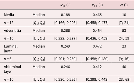
n indicates the number of samples measured for the respective layer.
The luminal layers of AAA samples were even more circumferentially oriented and did not differ significantly from the medias in healthy tissue (p = 0.55), with α LL = ±23° [9; 46]. The in-plane dispersion of the luminal layer was also not significantly higher than that of the healthy media (p = 0.08), with κ ip,LL = 0.249 [0.201; 0.259]. In addition, the out-of-plane dispersion of the healthy media and the LL of AAA, κ op,LL = 0.472 [0.458; 0.480], were not significantly different (p = 0.11). The AL of AAA did not differ significantly from the adventitia in terms of the mean fiber direction, α AL = ±40° [23; 68] (p = 0.73), the in-plane dispersion, κ ip,AL = 0.246 [0.230; 0.295] (p = 0.73), and the out-of-plane dispersion, κ op,AL = 0.412 [0.398; 0.443] (p = 0.10). Finally, the AL, compared to the luminal layer, showed no significant difference in all orientation (p = 0.26), in-plane (p = 0.88), and out-of-plane (p = 0.06) dispersion parameters.
Correlations Between Measures of Diameter, Waviness, Orientation, and Dispersion
For all healthy abdominal aortic samples, correlations between the dispersion parameters κ ip and both tortuosity and amplitude could be identified (all p-values < 0.03). The in-plane dispersion was positively correlated with the amplitude (r = 0.60, p = 0.01) and tortuosity (r = 0.51, p = 0.03), whereas the out-of-plane dispersion was negatively correlated with both the amplitude (r = −0.54, p = 0.02) and the tortuosity (r = −0.55, p = 0.02). In addition, the out-of-plane dispersion was negatively correlated with the diameter (r = −0.69, p = 0.001), whereas the diameter was positively correlated with the amplitude and tortuosity (both r = 0.78, p < 0.001).
Aneurysmal samples showed only significant correlations for out-of-plane dispersion with amplitude (r = −0.54, p = 0.04) and tortuosity (r = −0.58, p = 0.03). In addition, the p-value for both was higher than the corresponding p-value for the healthy samples. Figure 15 shows scatter plots of the amplitude versus the diameter for healthy and aneurysmal samples.

Fig. 15. Relationship between the amplitude A and the diameter D for (a) the healthy media (black solid dots) and the adventitia (red circles) and (b) the aneurysmal LL (black solid dots) and the AL (red circles).
Discussion
In this study, differences in collagen fiber diameter and waviness were demonstrated between healthy and aneurysmal abdominal aortas. The limitation of this study is a load-free state of the aortic wall during imaging. Consequently, the differences shown apply to the load-free state and may differ for the in vivo state. Considering that the mechanical behavior of an aortic wall changes with aneurysm progression (Niestrawska et al., Reference Niestrawska, Regitnig, Viertler, Cohnert, Babu and Holzapfel2019) and collagen waviness changes with increasing loading (Chow et al., Reference Chow, Turcotte, Lin and Zhang2014; Krasny et al., Reference Krasny, Morin, Magoariec and Avril2017; Pukaluk et al., Reference Pukaluk, Wolinski, Viertler, Regitnig, Holzapfel and Sommer2021), analysis of collagen waviness in the in vivo conditions could be of interest for future studies.
The diameter of the collagen fibers was previously measured by Chen et al. (Reference Chen, Liu, Slipchenko, Zhao, Cheng and Kassab2011, Reference Chen, Slipchenko, Liu, Zhao, Cheng, Lanir and Kassab2013) in the fresh porcine coronary adventitia, and Pickering et al. (Reference Pickering, Ford and Chow1996) documented diameters on atherosclerotic human samples. The healthy porcine adventitia had a mean fiber diameter of 2.8 μm (Chen et al., Reference Chen, Liu, Slipchenko, Zhao, Cheng and Kassab2011, Reference Chen, Slipchenko, Liu, Zhao, Cheng, Lanir and Kassab2013), which is very similar to the healthy human medial fiber diameter of 3.0 μm measured in our study. A comparison between healthy porcine adventitia and healthy human adventitia is not possible because we measured the diameter of clearly formed collagen bundles and not fibers. However, we have observed both fibers and bundles in the aneurysmal adventitia. The fibers of the aneurysmal adventitia were thicker than those reported in healthy porcine samples (Chen et al., Reference Chen, Liu, Slipchenko, Zhao, Cheng and Kassab2011, Reference Chen, Slipchenko, Liu, Zhao, Cheng, Lanir and Kassab2013) and healthy human samples from our study, as can be seen from the diameter distribution in Figure 7. The value of the first quartile from the aneurysmal abluminal layer, see Figure 6 and Table 1, is also higher than the diameter of healthy collagen fibers in healthy arterial and aortic samples. This observation of thicker collagen fibers in the aneurysmal abdominal layer has already been pointed out by Niestrawska et al. (Reference Niestrawska, Viertler, Regitnig, Cohnert, Sommer and Holzapfel2016) and Urabe et al. (Reference Urabe, Hoshina, Shimanuki, Nishimori, Miyata and Deguchi2016). In addition, the thicker fibers in the atherosclerotic human adventitia with a mean fiber diameter of 9.2 μm were previously reported by Pickering et al. (Reference Pickering, Ford and Chow1996). This similarity between atherosclerotic and aneurysmal collagen fibers seems plausible, since AAA is often associated with atherosclerosis (Golledge & Norman, Reference Golledge and Norman2010).
Rezakhaniha et al. (Reference Rezakhaniha, Agianniotis, Schrauwen, Griffa, Sage, Bouten, van de Vosse, Unser and Stergiopulos2012) quantified the waviness of adventitial collagen in the carotid arteries of rabbits using the straightness parameter. Their mean measured straightness parameter was 0.72, which corresponds to the tortuosity of 1.39. Although the samples were taken from different species, in a different location, the tortuosity of collagen from the rabbit carotid adventitia is quite similar compared to the median tortuosity of collagen bundles in the healthy abdominal aortic adventitia that we found (T A = 1.41). The similarities are not limited to the mean and median values, but extend to the distributions. Rezakhaniha et al. (Reference Rezakhaniha, Agianniotis, Schrauwen, Griffa, Sage, Bouten, van de Vosse, Unser and Stergiopulos2012) fitted their data to the beta distribution with estimated α = 4.47 and β = 1.76, which are very similar to α = 4.84 and β = 1.59 for the healthy human aortic adventitia, as analyzed in our study. In addition, the extreme value distribution for the adventitia shows surprisingly similar estimated parameters, that is, μ = 0.800 and σ = 0.133 for the rabbit's carotid artery versus μ = 0.824 and σ = 0.123 for the human aorta.
The obtained and quantified values of the geometrical parameters of the collagen fibers and bundles imply a considerable remodeling on the micro-scale level. Some significant differences in diameter, amplitude, and tortuosity are summarized in Figure 16. While the diameter of the collagen fibers in the medial layer was significantly different compared to the collagen bundles in the adventitia, there was not much difference between the luminal and abluminal AAA layers. In addition, the collagen diameter showed no difference between the luminal layer and the adventitia, suggesting remodeling of the luminal layer, which tends to the micro-architecture observed in the healthy adventitia. In addition to the collagen diameter, the waviness parameters between the layers of the aneurysmal aortic wall became more similar. As can be seen from Figure 11, the layers become less distinguishable as the amplitude of the collagen wave decreases, especially when looking at the abluminal side. However, the tortuosity of the abluminal layer is still significantly higher than that of the luminal layer. Based on the values of the diameter (Figure 6) and waviness (Figure 7) shown in the box-and-whisker plots, the parameters of the luminal layer were in between the medial and adventitial parameters. The parameters of the AL were also in between the medial and adventitial parameters. This observation suggests that both layers have undergone remodeling; in addition, the aneurysmal aortic wall lost its layer-specific character and tended to become a homogeneous structure.
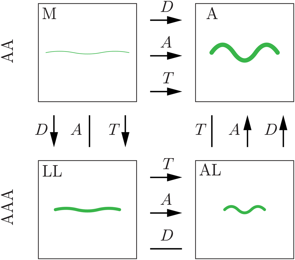
Fig. 16. Summary of the significant differences in diameter D, amplitude A, and tortuosity T, found in the present study. An average collagen fiber is shown schematically (in green) for the media (M) and adventitia (A) of healthy samples (AA) and the LL and the AL of aneurysmal samples (AAA). Significant differences between the layers are indicated by arrows pointing to the layer with the higher parameter value. Straight lines (no arrow) indicate no significant difference between the layers.
In contrast, the waviness parameters indicate that the main remodeling occurred on the abluminal side. The end-point distance in the abluminal layer was significantly smaller compared to the healthy adventitia. The amplitude was significantly lower in the aneurysmal abluminal layer than that in the adventitia. These simultaneous changes in both end-point distance and amplitude did not result in a significant difference in tortuosity. Therefore, we hypothesize that the fiber bundles on the abluminal side become more curly and lose their smooth waves to a more curled appearance (see Figure 5 for exemplary images of a healthy adventitia and an aneurysmal AL).
Conclusions
To the best of our knowledge, our comparative study is the first to provide a data set of measurements of collagen diameter and waviness, as well as orientation and dispersion for healthy and aneurysmal abdominal aortas, which can be further used to improve material and multiscale models of aortic walls and aneurysm formation.
Acknowledgments
The authors thank the Institute of Science and Technology Austria in Klosterneuburg for support with SHG imaging. Special thanks go to the contribution of the master's student C. Towler from the University of Glasgow for her work on the integration of MATLAB and ImageJ for the quantification of collagen fibers as well as M. Dalbosco from the Institute of Biomechanics, TU Graz for helpful discussions. Supported by TU Graz Open Access Publishing Fund.
Conflict of interest
The authors declare that they have no known competing financial interests or personal relationships that could have appeared to influence the work reported in this paper.


 Open access