


Contents
1 Introduction 2
1.1 Map of the paper 3
2 Some Background 4
2.1 What this paper is (not) about 4
2.2 Basic data structures 5
2.3 The permutation action 6
3 Idealised EUTxO:
 $\textsf{IEUTxO}$
7
$\textsf{IEUTxO}$
7
3.1 IEUTxO equations and solutions 7
3.2 Positions 10
3.3 Why we have
 $\alpha$
and
$\alpha$
and
 $\beta$
11
$\beta$
11
3.4 Chunks and blockchains 12
3.4.1 Chunks 12
3.4.2 UTxOs, UTxIs …. 13
3.4.3 …. and blockchains 14
3.5 Properties of chunks and blockchains 16
3.5.1 Algebraic and closure properties of chunks 17
3.5.2 Some observations on observational equivalence 17
3.5.3 Properties of UTxOs and UTxIs 19
3.6 An application: UTxO systems are ‘Church-Rosser’, in a suitable sense 19
3.7 The category
 $\textsf{IEUTxO}$
of IEUTxO models 20
$\textsf{IEUTxO}$
of IEUTxO models 20
3.8 Idealised UTxO 21
4 Abstract Chunk Systems:
 $\textsf{ACS}$
22
$\textsf{ACS}$
22
4.1 Basic definitions 22
4.2 Monoid of chunks 23
4.3 Behaviour, positions and equivalence 25
4.3.1 Left and right behaviour 25
4.3.2 Positions 26
4.3.3 Observational equivalence 28
4.4 Oriented monoids 29
4.4.1 Definition and properties 29
4.4.2 A brief discussion 31
4.5 The category
 $\textsf{ACS}$
of abstract chunk systems 32
$\textsf{ACS}$
of abstract chunk systems 32
4.6 Examples of abstract chunk systems 33
5 The Functor
 $F:\textsf{IEUTxO}\to\textsf{ACS}$
34
$F:\textsf{IEUTxO}\to\textsf{ACS}$
34
5.1 Action on objects 34
5.2 Relation between the partial monoid
 $\textsf{Chunk}_{\mathbb T}$
and the monoid of chunks
$\textsf{Chunk}_{\mathbb T}$
and the monoid of chunks
 $F(\mathbb T)$
35
$F(\mathbb T)$
35
5.3
 $F(\mathbb T)$
is oriented, so
$F(\mathbb T)$
is oriented, so
 $F(\mathbb T)\in\textsf{ACS}$
in ACS 36
$F(\mathbb T)\in\textsf{ACS}$
in ACS 36
5.4 Action of FF on arrows 37
5.5 Blocked channels 38
6 The Functor
 $G:\textsf{ACS}\to\textsf{IEUTxO}$
39
$G:\textsf{ACS}\to\textsf{IEUTxO}$
39
6.1 A brief discussion: why represent? 40
6.2 Action on objects 42
6.3
 $\nu$
is injective 42
$\nu$
is injective 42
6.4 Action on arrows 42
7 An Adjunction between
 $F:\textsf{IEUTxO}\to\textsf{ACS}$
and
$F:\textsf{IEUTxO}\to\textsf{ACS}$
and
 $G:\textsf{ACS}\to\textsf{IEUTxO}$
43
$G:\textsf{ACS}\to\textsf{IEUTxO}$
43
7.1 The counit map
 $\epsilon_{\textsf X}:FG(\textsf X)\to\textsf X$
exists and is a surjection 43
$\epsilon_{\textsf X}:FG(\textsf X)\to\textsf X$
exists and is a surjection 43
7.2 The unit map
 $\eta_{\mathbb T}:\mathbb T\to \mathrm{GF}(\mathbb T)$
exists and is an isomorphism 44
$\eta_{\mathbb T}:\mathbb T\to \mathrm{GF}(\mathbb T)$
exists and is an isomorphism 44
7.3 FF is left adjoint to GG 45
8 Conclusions 47
8.1 Observational equivalence 48
8.2 Garbage collection 48
8.3 Tests 49
8.4 Connections with nominal techniques 50
8.5 Concrete formalisation 51
8.6 Future work 52
8.7 Final words 52
1. Introduction
Blockchain is a young field – young enough that no consensus has yet developed as to its underlying mathematical structures. There are many blockchain implementations, but what (mathematically) are they implementations of?
-
• Two major blockchain architectures exist:
-
• UTxO-based blockchains (like Bitcoin) and accounts-based blockchains (like Ethereum).
We consider UTxO style blockchains in this paper, and specifically the Extended UTxO style model (Chakravarty et al. Reference Chakravarty, Chapman, MacKenzie, Melkonian, Peyton Jones and Wadler2020), which as the name suggests extends the UTxO structure (how, is described in Remark 3.8.1) of Bitcoin, which is still the canonical blockchain application.
So our question becomes: what, mathematically speaking, is an EUTxO blockchain?
In the literature, Figure 3 of Chakravarty et al. (Reference Chakravarty, Chapman, MacKenzie, Melkonian, Peyton Jones and Wadler2020) exhibits Extended UTxO as an inductive data type, designed with implementation and formal verification in mind. Most blockchains exist only in code, so to have an inductive specification to work from in a published academic paper is a luxury for which we can be grateful.
However, this does not answer our question.
It would be like answering “What are numbers?” with the inductive definition
 $\mathbb N= 1 + \mathbb N$
: this an important structure (and to be fair, it yields an important inductive principle) but this does not tell us that
$\mathbb N= 1 + \mathbb N$
: this an important structure (and to be fair, it yields an important inductive principle) but this does not tell us that
 $\mathbb N$
is a ring; or about primes and the fundamental theorem of arithmetic; or that
$\mathbb N$
is a ring; or about primes and the fundamental theorem of arithmetic; or that
 $\mathbb N$
is embedded in
$\mathbb N$
is embedded in
 $\mathbb Q$
and
$\mathbb Q$
and
 $\mathbb R$
; or even about binary representations. In short, Figure 3 of Chakravarty et al. (Reference Chakravarty, Chapman, MacKenzie, Melkonian, Peyton Jones and Wadler2020) gives us the raw data structure of one particular blockchain implementation, which is certainly important, but this is not a mathematics of blockchains.
$\mathbb R$
; or even about binary representations. In short, Figure 3 of Chakravarty et al. (Reference Chakravarty, Chapman, MacKenzie, Melkonian, Peyton Jones and Wadler2020) gives us the raw data structure of one particular blockchain implementation, which is certainly important, but this is not a mathematics of blockchains.
As we shall see, there is more to be said here.
1.1 Map of the paper
A map of this paper, and our answer, is as follows:
-
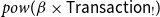
(1). In Section 3, we present Idealised EUTxO (Definition 3.1.1), which is four type equations (Figure 1). This captures the essence of Chakravarty et al. (Reference Chakravarty, Chapman, MacKenzie, Melkonian, Peyton Jones and Wadler2020, Figure 3), but far more succinctly – four lines vs. one full page. Footnote 1 So, EUTxO is a solution to the IEUTxO equations in Figure 1.

Figure 1. Type equations of Idealised EUTxO.
-
(2). The approach to blockchain in this paper is novel – we concentrate not on blockchains but on blockchain segments, which we call chunks (Definition 3.4.1). Chunks have many properties that blockchains do not have: if you cut a blockchain into pieces you get chunks, not blockchains; and chunks have more structure, for example they form a partially ordered partial monoid (Theorem 3.5.4) which communicate across channels (much like the
$\pi$
-calculus Milner Reference Milner1999) and they display resource separation properties reminiscent of known systems such as separation logic (Remark 3.5.13). A blockchain is the special case of a chunk with no active input channels (Definition 3.4.10). So, EUTxO is a system of chunks (a partially-ordered partial monoid with channels). -
(3). IEUTxO models form a category (Definition 3.7.1). So now, EUTxO is the category of partially ordered partial monoid solutions to the IEUTxO models and arrows between them.
-
(4). Our answers are still quite concrete, in the sense that objects are solutions to type equations. To go further, we use algebra. We introduce abstract chunk systems (Definition 4.5.1), which are oriented atomic monoids of chunks (Definitions 4.4.1, 4.2.5, and 4.2.1). These too form a category (Definition 4.5.2), with objects and arrows. Thus, we extract relevant properties of what makes solutions to the IEUTxO equations in Figure 1 interesting, as explicit and testable algebraic properties (see the discussion in Subsection 8.3). Several design choices exist in this space: we discuss some of them in Remarks 6.4.4 and 7.1.5 and Proposition 7.3.6.So now EUTxO is a bundle of abstract algebraic, testable properties, which exists in a clean design space which could be explored in future work.
-
(5). Finally, we pull this all together by constructing functors between the categories of IEUTxO models and of abstract chunk systems (Definitions 5.1.1 and 6.2.1), and we exhibit a cycle of categorical embeddings between them (Theorem 7.3.4). So finally, EUTxO becomes a pair of categories – one of concrete solutions to some type equations, and this embedded in a category of abstract algebras – related by adjoint functors mapping between them; or if the reader prefers, it becomes a loop of embeddings (illustrated in Remark 7.3.5), cycling between the concrete and abstract algebras.


There are many definitions and results in this paper, and this leads to a broader point of it: that the mathematics we observe is possible. There is a mathematics of blockchain here which we have not seen commented on before.
This may help make blockchain more accessible and interesting to a mathematical audience and improve communication – since there is no more effective language for handling complexity than mathematics. Furthermore, as we argue in Subsections 4.4.2 and 8.3, our analysis of blockchain structure in this paper is not just of interest to mathematicians – it may also be of practical interest to programmers – by suggesting ways to structure and transform code, and establishing properties for unit tests, property-based testing and formal verification of correctness – and to designers of new UTxO-based systems, wishing to attain good design and security by working from a (relatively compact) mathematical reference model.
More exposition and discussion is in the body of the paper and in Section 8, including discussions of future work. Footnote 2
2. Some Background
2.1 What this paper is (not) about
We are parametric across possible data.
Blockchains are best-known as stores of value but it is widely appreciated in the industry that a blockchain is just a particular kind of distributed database and that the data stored on it, and consistency conditions imposed on its transactions, can vary with the application.
This paper (in common with many real-life blockchain implementations) is parametric in the type of data stored on it. Specifically, we include as a parameter an uninterpreted type
 $\beta$
of ‘data’ in our ‘Idealised IEUTxO’, as a user-determined black box, and we admit a choice of admissible transactions and validators (this is the subset inclusions in the last two lines of Figure 1).
Footnote 3
$\beta$
of ‘data’ in our ‘Idealised IEUTxO’, as a user-determined black box, and we admit a choice of admissible transactions and validators (this is the subset inclusions in the last two lines of Figure 1).
Footnote 3
We do not consider networks or security.
Real blockchains rightly work hard to be efficient and secure. In the real world, we hash data, network latency matters, as do good cryptography, incentives, permissions, user training, passwords, privacy, and more.
Again, we are parametric in these concerns. We include an uninterpreted type
 $\alpha$
of ‘keys’, but do not force any particular cryptographic content on them.
Footnote 4
$\alpha$
of ‘keys’, but do not force any particular cryptographic content on them.
Footnote 4
We do have validators, but we elide their computational content.
The UTxO model of adding a block to a chain is that the chain has ‘unspent outputs’ – meaning output ports that have not yet engaged in interaction – and at each unspent output o is located at some data d and a validator v.
A validator is a machine that takes data-key pairs as input and decides whether they are ‘good’ or ‘bad’. Good data-key pairs let the user interact with the blockchain; bad ones get rejected. In more detail, to append a block to the blockchain, we
-
• find a validator v on an unspent output o with data d and present it with a suitable key k such v considers (d,k) to be ‘good’;
-
• the output is now considered ‘spent’ and our block is attached to the chain. Footnote 5
This is much like putting a key into a lock to open a door, except that appending a block is irreversible: an output, once spent, cannot be unspent. Footnote 6 The idea is that our newly attached block may introduce fresh outputs with validators which we designed and to which we have the keys; Footnote 7 these are new ‘unspent’ outputs on the chain. Footnote 8
We do model validators in this paper, but mathematically – meaning that a validator is not a code-script (as it would be in real life). Instead, we identify a validator directly with the set of data-key pairs that it accepts.Footnote 9
Remark 2.1.1 In summary: Idealised (E)UTxO is a mathematical model of the structural act of UTxO block combination and validation and Abstract chunk systems are an algebraic rendering of the same idea.
This basic idea of block combination and validation might not seem like much. Footnote 10 However, this is the fundamental operation of the UTxO architecture, and we shall find many interesting and unexpected observations to make about it.
So if there is one question that this paper addresses, it is this: What does it mean, mathematically, when we append a transaction to a UTxO blockchain?
Our answer occupies the rest of this paper.
In the rest of this Section, we will set up some basic mathematical machinery. The reader is welcome to skip or skim it and refer back to it as required.
2.2 Basic data structures
Definition 2.2.1
-
(1). Fix a countably infinite set
${\mathbb A}=\{a,b,c,p,\dots\}$
of atoms. -
(2). A permutation is a bijection on
${\mathbb A}$
; write
$\pi,\pi'\in\textit{Perm}$
for permutations.


Remark 2.2.2 Following the ideas in Gabbay (2020a), Gabbay and Pitts (2001) atoms will be the atoms of ZFA of Zermelo-Fraenkel set theory with Atoms
Footnote 11
– this is a fancy way to say that
 ${\mathbb A}$
is a type of atomic identifiers.
${\mathbb A}$
is a type of atomic identifiers.
We will use atoms to locate inputs and outputs on a blockchain. More on this in Subsection 2.3.
Notation 2.2.3
-
(1). Write
$\mathbb N=\{0,1,2,\dots\}$
. -
(2). If
$\textsf X$
is a set, write
$\textit{fin}(\textsf X)$
for the finite power set of
$\textsf X$
, and
$\textit{fin}_!(\textsf X)$
for the pointed finite power set. In symbols: Above, (X,x) is a pair, and
\begin{align*}\textit{fin}_!(\textsf X) = \{ (X,x)\in \textit{fin}(\textsf X)\times \textsf X\mid x\in X\}.\end{align*}
$\textit{fin}(\textsf X)\times\textsf X$
is a Cartesian product.
-
(3). If
$\textsf X$
and
$\textsf Y$
are sets, we use a convenient shorthand in Figure 1 by writing That is, we take
\begin{align*}(\textit{fin}(\textsf X),\textsf Y)_!\quad\text{as shorthand for}\quad(\textit{fin}(\textsf X)_!,\textsf Y) .\end{align*}
$(\text{-})_!$
to act on a pair functorially, on the first component. We do this in Figure 1 when we write
$\textsf{Transaction}_!$
in the definition of
$\textsf{Validator}$
.
-
(4). If
$\textsf X$
is a set then write
$[\textsf X]$
for the set of (possibly empty) finite lists of elements from
$\textsf X$
. We write
$\bullet$
for list concatenation, so
$l\bullet l'$
is l followed by l’. More generally, we will write
$\bullet$
for any monoid composition; list concatenation is one instance. It will always be clear what is intended. -
(5). If
$\textsf X$
is a set then order
$l,l'\in [\textsf X]$
by the sublist inclusion relation, where
$l\leq l'$
when l can be obtained from l’ by deleting (but not rearranging) some of its elements. -
(6). If
$\textsf X$
is a set and
$x\in\textsf X$
then we may call the one-element list
$[x]\in[\textsf X]$
a singleton. -
(7). If
$V\in \textsf X\to\textsf{Bool}$
and
$x\in\textsf X$
then we may write V(x) or
$V\,x$
for
$V\,x = \textsf{True}$
.


2.3 The permutation action
Remark 2.3.1 We spend this Subsection introducing permutations and their action on elements. We will need this most visibly in two places:
-
(1). To state the key Definition 4.3.6.
-
(2). To prove Lemma 5.2.1, and thus Proposition 5.2.2.
Because we assume atoms and are working in a ZFA universe, everything has a standard permutation action. We describe it in Definition 2.3.3. Programmers can think of the permutation action as a generic definition in the ZFA universe (given below in this Remark), which is sufficiently generic that it exists for all the data types considered in this paper. By this perspective, Definition 2.3.3 specifies how this generic action interacts with the specific type-formers of interest for this paper.
Definition 2.3.2 For reference, we write out the ZFA generic definition, which is by
 $\epsilon$
-induction on the sets universe:
$\epsilon$
-induction on the sets universe:
 \begin{align*}\begin{array}{r@{\ }l@{\qquad}l}\pi{\cdot} a=&\pi(a) & a\in{\mathbb A}\\\pi{\cdot} X =& \{\pi{\cdot} x\mid x\in X\} &X\text{ a set}.\end{array}\end{align*}
More information on this sets inductive definition is in Gabbay (Reference Gabbay2001, Reference Gabbay2020a). Definition 2.3.3 can be usefully viewed as a collection of concrete instances of Definition 3.2 for the data types of interest in this paper:
Definition 2.3.3 Permutations
 $\pi$
act concretely as follows:
$\pi$
act concretely as follows:
-
(1). If
$\pi\in\textit{Perm}$
and
$a\in\mathbb A$
then
$\pi$
acts on a as a function:
\begin{align*}\pi{\cdot} a=\pi(a) .\end{align*}
-
(2). If
$\pi\in\textit{Perm}$
and X is any set then
$\pi$
acts pointwise on X as follows: Note as a corollary of this that
\begin{align*}\pi{\cdot} X=\{\pi{\cdot} x\mid x\in X\} .\end{align*}
$x\in X \Longleftrightarrow \pi{\cdot} x\in\pi{\cdot} X$
.
-
(3). If
$\pi\in\textit{Perm}$
and
$(x_1,\dots,x_n)$
is a tuple then
$\pi$
acts pointwise on
$(x_1,\dots,x_n)$
as follows: Note therefore that
\begin{align*}\pi{\cdot}(x_1,\dots,x_n) = (\pi{\cdot} x_1,\dots,\pi{\cdot} x_n) .\end{align*}
$\pi{\cdot}((x_1,\dots,x_n)!!i)=\pi{\cdot} x_i$
, where
$1\leq i\leq n$
and
$!!$
indicates lookup.
-
(4). If
$\pi\in\textit{Perm}$
and
$i\in\mathbb N$
then
$\pi{\cdot} i = i$
. -
(5). If
$\pi\in\textit{Perm}$
and (X,x) is a pointed set (Notation 2.2.3(2)) then
$\pi$
acts pointwise on (X,x) as follows: (This is indeed just a special case of the previous case, for tuples.) If
\begin{align*}\pi{\cdot} (X,x) = (\pi{\cdot} X,\pi{\cdot} x) .\end{align*}
$\pi\in\textit{Perm}$
and f is a function, then
$\pi$
has the conjugation action on f as follows: Note therefore that
\begin{align*}(\pi{\cdot} f)(x) = \pi{\cdot}(f(\pi^{\text{-}1}{\cdot} x)) .\end{align*}
$\pi{\cdot} (f(x))=(\pi{\cdot} f)(\pi{\cdot} x)$
, and
$\pi{\cdot} f$
maps
$\pi{\cdot} x$
to
$\pi{\cdot} (f(x))$
.
-
(6). In particular,
$\pi$
acts as the above on the inputs, outputs, sets of inputs, sets of outputs, transactions, and validators from Figure 1. -
(7). If
$\pi\in\textit{Perm}$
and R is a relation, then
$\pi$
acts pointwise such that so that
\begin{align*}\pi{\cdot} R = \{(\pi{\cdot} x,\pi{\cdot} y)\mid (x,y)\in R\}\end{align*}
\begin{align*}x\mathrel{\pi{\cdot} R} y\Longleftrightarrow\pi^{\text{-}1}{\cdot} x\mathrel{R} \pi^{\text{-}1}{\cdot} y .\end{align*}


We use Definition 2.3.4 in Definition 4.3.6, but it is a useful concept so we include it here:
Definition 2.3.4 If
 $a\in{\mathbb A}$
then write
$a\in{\mathbb A}$
then write
 $\textit{fix}(a)$
for the set of permutations
$\textit{fix}(a)$
for the set of permutations
 $\pi\in\textit{Perm}$
such that
$\pi\in\textit{Perm}$
such that
 $\pi(a)=a$
. In symbols:
$\pi(a)=a$
. In symbols:
 \begin{align*}\textit{fix}(a) = \{\pi\in\textit{Perm} \mid \pi(a)=a\} .\end{align*}
Definition 2.3.5 Call an element equivariant when
 $\pi{\cdot} x=x$
for every
$\pi{\cdot} x=x$
for every
 $\pi\in\textit{Perm}$
. Concretely:
$\pi\in\textit{Perm}$
. Concretely:
-
(1).
${\mathbb A}$
is equivariant, and no individual atom
$a\in{\mathbb A}$
is equivariant. -
(2). A set X is equivariant when
In words: A set is equivariant precisely when it is closed in the orbits of its elements under the permutation action.
\begin{align*}\forall{\pi{\in}\textit{Perm}}(x\in X \Longleftrightarrow \pi{\cdot} x\in X).\end{align*}
-
(3).
$(x_1,\dots,x_n)$
is equivariant precisely when
$x_i$
is equivariant for every
$1\leq i\leq n$
. -
(4).
$\mathbb N$
is equivariant, and every
$i\in\mathbb N$
is equivariant. -
(5). A pointed set (X,x) is equivariant precisely when X and x are equivariant.
-
(6). A function f is equivariant when
$\pi{\cdot} (f(x))=f(\pi{\cdot} x)$
for every x and every
$\pi$
. -
(7). A relation R is equivariant when
\begin{align*}\forall{\pi{\in}\textit{Perm}}\forall{x,y}(x\mathrel{R} y \Longleftrightarrow \pi{\cdot} x\mathrel{R}\pi{\cdot} y) .\end{align*}


3. Idealised EUTxO:
$\textsf{IEUTxO}$

3.1 IEUTxO equations and solutions
Definition 3.1.1 Let idealised EUTxO be the type equations in Figure 1 (
 $\textsf{Transaction}_!$
is from Notation 2.2.3(3)).
$\textsf{Transaction}_!$
is from Notation 2.2.3(3)).
Definition 3.1.2 Let a solution or model of the IEUTxO type equations in Figure 1 be a tuple
 \begin{align*}\mathbb T=(\alpha,\beta,\textsf{Transaction},\textsf{Validator},\nu : \textsf{Validator}\hookrightarrow \textit{pow}(\beta\times\textsf{Transaction}_!))\end{align*}
where
-
(1).
$\alpha$
is an uninterpreted
Footnote 12
equivariant (Definition 2.3.5(2)) set of keys, -
(2).
$\beta$
is an uninterpreted equivariant set of data, -
(3).
$\textsf{Validator}$
is an equivariant set of validators. -
(4).
$\textsf{Transaction}$
is an equivariant subset of
$\textit{fin}({\mathbb A}\times\alpha)\times\textit{fin}({\mathbb A}\times\beta\times\textsf{Validator}),$
and we disallow the empty transaction, having no inputs or outputs. -
(5).
$\nu$
is an equivariant injective function (Definition 2.3.5(3)) from
$\textsf{Validator}$
to
$\textit{pow}(\beta\times\textsf{Transaction}_!)$
.


Some notation will be helpful:
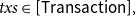
Notation 3.1.3 If
 $\textit{tx}=(I,O)\in\textsf{Transaction}$
and
$\textit{tx}=(I,O)\in\textsf{Transaction}$
and
 $i\in I$
then write
$i\in I$
then write
 $\textit{tx}\text{@} i\in\textsf{Transaction}_!$
for the input-in-context ((I,i),O) obtained by pointing I at
$\textit{tx}\text{@} i\in\textsf{Transaction}_!$
for the input-in-context ((I,i),O) obtained by pointing I at
 $i\in I$
(Notation 2.2.3). In symbols:
$i\in I$
(Notation 2.2.3). In symbols:
 \begin{align*}\text{if }\textit{tx}=(I,O)\in\textsf{Translation}\ \text{and}\ i\in I\quad\text{then}\quad\textit{tx}\text{@} i = ((I,i),O) \in \textsf{Transaction}_!\end{align*}
Example 3.1.4 In Figures 2 and 3, we take a short diagrammatic tour of Definition 3.1.2, before continuing with the technical development. Since we have yet to build our machinery, this discussion is informal and intuitive. We include precise forward pointers to later definitions where appropriate; additional diagrams will be discussed in detail in Example 3.4.11.
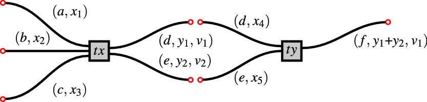
Figure 2. A pair of transactions
 $\textit{tx}$
and
$\textit{tx}$
and
 $\textit{ty}$
.
$\textit{ty}$
.
 $\textit{tx}\in\textsf{Transaction}$
in Figure 2 is a pair of a set of three inputs, and a set of two outputs:
$\textit{tx}\in\textsf{Transaction}$
in Figure 2 is a pair of a set of three inputs, and a set of two outputs:
 \begin{align*}\textit{tx}\ =\ \Bigl(\{(a,x_1),(b,x_2),(c,x_3)\}\ ,\ \{(d,y_1,v_1),(e,y_2,v_2)\}\Bigr) .\end{align*}
Above:
-
• a, b, c, d and e are atoms in
$\mathbb A$
. They serve as unique labels for the inputs and outputs. Note that every input and output in
$\textit{tx}$
has a distinct label. This is not directly enforced in the raw data type in Figure 1, but it will follow as a consequence of well-formedness conditions which we introduce later, in Definition 3.4.1. Since each input is labelled with a unique atom, and similarly for each output, we may treat atoms as positions, locations or channels. Thus for example, the input
$(a,x_1)$
is labelled with a and so we can think intuitively that it is located at position a; or waiting to communicate its data
$x_1$
on channel a. -
•
$x_1$
and
$x_2$
are elements of
$\alpha$
. This is just an uninterpreted data type, but a good intuition is that these are cryptographic keys. -
•
$y_1$
and
$y_2$
are elements of
$\beta$
. This is just an uninterpreted data type: the intuition is that
$y_1$
and
$y_2$
are fragments of state data. Note that state data are stored per-output and not per-transaction. We suppose for concreteness that
$\beta=\mathbb N$
, so state data can be summed (as we do in the output f of
$\textit{ty}$
; more in this shortly). Note that
$\textsf{Transaction}$
is a subset of
$\textit{fin}(\textsf{Input})\times\textit{fin}(\textsf{Output})$
in Figure 2; which subset, is a parameter of the model selected. So for example, we could enforce that all state data on all inputs and outputs should be equal, and this would in effect ensure that state data are a per-transaction quantity. This may or may not be what we want: the definition allows us to choose. -
•
$v_1$
and
$v_2$
are validators. Their role is, intuitively, to decide which transactions
$\textit{tx}$
will interact with (precise definition in Definition 3.4.1(4)).


 $\textit{ty}\in\textsf{Transaction}$
is another transaction, with two inputs and one output. Note that its inputs are located at d and e, meaning that the inputs of
$\textit{ty}\in\textsf{Transaction}$
is another transaction, with two inputs and one output. Note that its inputs are located at d and e, meaning that the inputs of
 $\textit{ty}$
point to the outputs of
$\textit{ty}$
point to the outputs of
 $\textit{tx}$
(Definition 3.2.6). Note also that it performs an addition, in the sense that the state data of its single output are the sum of the state data on its two inputs.
$\textit{tx}$
(Definition 3.2.6). Note also that it performs an addition, in the sense that the state data of its single output are the sum of the state data on its two inputs.
If in addition the following validation conditions are satisfied (@ from Notation 3.1.3)
-
•
$(y_1,\textit{ty}\text{@} (d,x_4))\in \nu(v_1)$
(in words: validator
$v_1$
in state
$y_1$
validates the pointed transaction
$\textit{ty}\text{@} (d,x_4))$
), and -
•
$(y_2,\textit{ty}\text{@} (e,x_5))\in \nu(v_2)$
(in words: validator
$v_2$
in state
$y_2$
validates the pointed transaction
$\textit{ty}\text{@} (e,x_5)$
) then the two-element sequence
$[\textit{tx},\textit{ty}]$
is considered to be a valid combination. In the terminology, we define later, this is called a chunk (Definition 3.4.1).
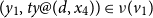


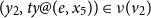


Supposing this is so. Then, we can join the two transactions as illustrated in Figure 3, using blue circles to indicate successful validations. Congratulations: we have performed our first blockchain concatenation.
Note that both validations must succeed for the combination
 $[\textit{tx},\textit{ty}]$
to be considered a valid chunk. More diagrams and discussion follow in Example 3.4.11. We now return to the definitions.
$[\textit{tx},\textit{ty}]$
to be considered a valid chunk. More diagrams and discussion follow in Example 3.4.11. We now return to the definitions.
Notation 3.1.5 Sets that do not include atoms – including
 $\mathbb N$
, inductive types built using
$\mathbb N$
, inductive types built using
 $\mathbb N$
, and function types built using
$\mathbb N$
, and function types built using
 $\mathbb N$
– are automatically equivariant. Thus, if the reader unfamiliar with nominal techniques and ZFA wonders whether particular choices they need for
$\mathbb N$
– are automatically equivariant. Thus, if the reader unfamiliar with nominal techniques and ZFA wonders whether particular choices they need for
 $\alpha$
,
$\alpha$
,
 $\beta$
and
$\beta$
and
 $\textsf{Validator}$
are equivariant – then the answer is ‘yes’.
$\textsf{Validator}$
are equivariant – then the answer is ‘yes’.
We may elide equivariance conditions Definition 3.1.2 henceforth. Any such type-like definition will be equivariant – that is closed under taking orbits of the permutation action – unless stated otherwise.
Remark 3.1.6 Equivariance comes from the underlying ZFA universe. Notation 1.5 can be viewed as an assertion that the definition exists in the category of equivariant ZFA sets and equivariant functions between them (or if the reader prefers: sets with a permutation action, and equivariant functions between them).
This paper will be light on sets and categorical foundations: we use just enough so that readers from various backgrounds get a hook on the ideas that speaks to them, and so it is always clear what is meant and how it could be made fully formal.
Note that just because a set is equivariant does not mean all its elements must be; for instance,
 $\mathbb A$
is equivariant (and consists of a single permutation orbit), but none of its elements
$\mathbb A$
is equivariant (and consists of a single permutation orbit), but none of its elements
 $a\in{\mathbb A}$
are equivariant.
$a\in{\mathbb A}$
are equivariant.
Remark 3.1.7 Compare Figure 1 with Chakravathy et al. (2020), Figure 3:
Footnote 13
 $\alpha$
here corresponds to redeemer there,
$\alpha$
here corresponds to redeemer there,
 $\beta$
here corresponds to datum there (though
$\beta$
here corresponds to datum there (though
 $\alpha$
here lives on inputs and
$\alpha$
here lives on inputs and
 $\beta$
lives on outputs, whereas there both redeemer and datum live on inputs); the by-hash referencing there is replaced here with a nominal treatment using atoms; and validators exist on the output here and on the input there. There is less to this latter difference (validator moving from input in Chakravathy et al. 2020 to output here) than meets the eye: what is key is the interaction between an output and a later input, so it a matter of perspective and our convenience whether we view the output as validating the input, or vice versa, or indeed both.
$\beta$
lives on outputs, whereas there both redeemer and datum live on inputs); the by-hash referencing there is replaced here with a nominal treatment using atoms; and validators exist on the output here and on the input there. There is less to this latter difference (validator moving from input in Chakravathy et al. 2020 to output here) than meets the eye: what is key is the interaction between an output and a later input, so it a matter of perspective and our convenience whether we view the output as validating the input, or vice versa, or indeed both.
Remark 3.1.8 Definition 3.1.2(4) uses a subset inclusion, whereas Definition 3.1.2(5) uses an injection
 $\nu$
. Why?irst, in practice we would expect
$\nu$
. Why?irst, in practice we would expect
 $\nu(v)$
to be a computable subset of
$\nu(v)$
to be a computable subset of
 $\beta\times\textsf{Transaction}_!$
, since we have implementations in mind (though nothing in the mathematics to follow will depend on this).
$\beta\times\textsf{Transaction}_!$
, since we have implementations in mind (though nothing in the mathematics to follow will depend on this).
Also, sets are well-founded, so a pure subset inclusion solution to Figure 1, for both clauses, would be difficult; we use
 $\nu$
to break the downward chain of sets inclusions.
Footnote 14
Yet just as we may write
$\nu$
to break the downward chain of sets inclusions.
Footnote 14
Yet just as we may write
 \begin{align*}\mathbb N\subseteq\mathbb Q\subseteq\mathbb R,\end{align*}
eliding (or neglecting to consider) that their realisations may differ (finite cardinals vs. equivalence classes of pairs vs. Dedekind cuts), so – since
 $\nu$
is an injection – it may be convenient to treat
$\nu$
is an injection – it may be convenient to treat
 $\textsf{Validator}$
as a literal subset of
$\textsf{Validator}$
as a literal subset of
 $\textit{pow}(\beta\times\textsf{Transaction}_!)$
.
Footnote 15
This is standard, provided we clearly state what is intended and are confident that we could unroll the injections if required.
$\textit{pow}(\beta\times\textsf{Transaction}_!)$
.
Footnote 15
This is standard, provided we clearly state what is intended and are confident that we could unroll the injections if required.
Thus, Definition 3.1.9 rephrases Definition 3.1.2, with a focus on extensional sets behaviour rather than on internal structure (and for reference, see Definition 6.2.1 for an example of where the internal structure is required):
Definition 3.1.9 An IEUTxO model
 $\mathbb T$
from Definition 3.1.2 can be presented modulo Remark 3.1.8 as a tuple
$\mathbb T$
from Definition 3.1.2 can be presented modulo Remark 3.1.8 as a tuple
 \begin{align*}\mathbb T=(\alpha_{\mathbb T},\beta_{\mathbb T},\textsf{Transaction}_{\mathbb T},\textsf{Validator}_{\mathbb T})\end{align*}
of sets that solves the equations in Figure 1. We may drop the
 $\mathbb T$
subscripts where these are clear from the context.
$\mathbb T$
subscripts where these are clear from the context.
3.2 Positions
Remark 3.2.1 The positions of a transaction are intuitively the interfaces or channels along which it may connect with other transactions to form a chunk (see next subsection). The notion of connection is called pointing to (Definition 3.2.6).
In Figure 3, the positions of
 $\textit{tx}$
and
$\textit{tx}$
and
 $\textit{ty}$
are
$\textit{ty}$
are
 $\{a,b,c,d,e\}$
and
$\{a,b,c,d,e\}$
and
 $\{d,e,f\},$
respectively, and input d of
$\{d,e,f\},$
respectively, and input d of
 $\textit{ty}$
points to output d of
$\textit{ty}$
points to output d of
 $\textit{tx}$
. Also,
$\textit{tx}$
. Also,
 $\textit{tx}$
is earlier than
$\textit{tx}$
is earlier than
 $\textit{ty}$
, and
$\textit{ty}$
, and
 $\textit{ty}$
is later than
$\textit{ty}$
is later than
 $\textit{tx}$
.
$\textit{tx}$
.
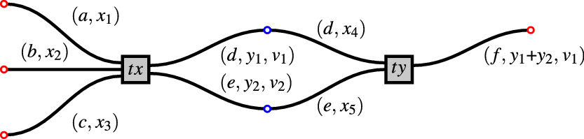
Figure 3. A pair of transactions
 $\textit{tx}$
and
$\textit{tx}$
and
 $\textit{ty}$
, successfully validated and combined.
$\textit{ty}$
, successfully validated and combined.
Notation 3.2.2
-
(1). If
$\textit{tx}\in\textsf{Transaction}$
appears in
$\textit{txs}\in[\textsf{Transaction}],$
then write
$\textit{tx}\in\textit{txs}$
. -
(2). If
$\textit{tx},\textit{tx}'\in\textit{txs}$
and
$\textit{tx}$
appears before
$\textit{tx}'$
in
$\textit{txs}$
, then call
$\textit{tx}$
earlier than
$\textit{tx}'$
and
$\textit{tx}'$
later than
$\textit{tx}$
(in
$\textit{txs}$
). -
(3). If
$\textit{tx}=(I,O)\in\textsf{Transaction}$
and
$o\in\textsf{Output}$
, say o appears in
$\textit{tx}$
and write
$o\in \textit{tx}$
when
$o\in O$
; similarly for an input
$i\in\textsf{Input}$
. We may silently extend this notation to larger data structures, writing for example
$i\in\textit{txs}$
when
$i\in\textit{tx}\in\textit{txs}$
for some
$\textit{tx}$
.


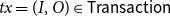


Definition 3.2.3 Suppose
 $\mathbb T$
is an IEUTxO model. We define positions of written
$\mathbb T$
is an IEUTxO model. We define positions of written
 $\textit{pos}$
as in Figure 4 (see also Definition 3.4.5).
$\textit{pos}$
as in Figure 4 (see also Definition 3.4.5).
Figure 4. Positions of (Definition 3.2.3).
Remark 3.2.4 Intuitively,
 $\textit{pos}(x)$
collects the positions mentioned explicitly on the inputs or outputs of a structure. Note that validators may also act depending on positions of their inputs, but this information is not detected by
$\textit{pos}(x)$
collects the positions mentioned explicitly on the inputs or outputs of a structure. Note that validators may also act depending on positions of their inputs, but this information is not detected by
 $\textit{pos}$
. For instance, consider a (arguably odd, but imaginable) output o having the form
$\textit{pos}$
. For instance, consider a (arguably odd, but imaginable) output o having the form
 \begin{align*}o=(b,0,\{i\in\textsf{Input} \mid \textit{pos}(i)=\{a\}\}) .\end{align*}
So this output is at position b,
 $\beta=\mathbb N$
and o carries data 0, and o has a validator that validates an input precisely when it is at position a. Then
$\beta=\mathbb N$
and o carries data 0, and o has a validator that validates an input precisely when it is at position a. Then
 $\textit{pos}(o)=\{b\}$
.Footnote 16
$\textit{pos}(o)=\{b\}$
.Footnote 16
Lemma 3.2.5 Suppose
 $\mathbb T$
is an IEUTxO model and
$\mathbb T$
is an IEUTxO model and
 $\textit{txs}\in[\textsf{Transaction}]$
. Then
$\textit{txs}\in[\textsf{Transaction}]$
. Then
 \begin{align*}\textit{pos}(\textit{txs})=\varnothing\quad\text{implies}\quad\textit{txs}=[].\end{align*}
Proof. Recall from Definition 3.1.2(4) that the empty transaction is disallowed. Now examining Figure 4, we see that the only way
 $\textit{txs}$
can mention no positions at all is by having no transactions and so being empty.
$\textit{txs}$
can mention no positions at all is by having no transactions and so being empty.
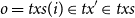
Definition 3.2.6
-
(1). Suppose
$i\in\textsf{Input}$
and
$o\in\textsf{Output}$
. Then say that i points to o and write
$i\mapsto o$
when they share a position: (The use of ‘point’ here is unrelated to the ‘pointed sets’ from Notation 2.2.3.)
\begin{align*}i\mapsto o \quad\text{when}\quad \textit{pos}(i)=\textit{pos}(o) .\end{align*}
-
(2). Recall the notation
$\textit{tx}\text{@} i$
from Notation 3.1.3. Suppose that: Then write
\begin{align*}\begin{array}{l}i=(p,k)\in{Input}\\i\in{tx}\in{Transaction}\ \ \text{and}\ \\ \phi=(p,d,V)\in{Output}.\end{array}\end{align*}
(1)and say that the output o validates the input-in-context
\begin{equation}{validates}(o,{tx}\text{@} i)\quad\text{when}\quad(d,{tx}\text{@} i) \in V\end{equation}
${tx}\text{@} i$
.


3.3 Why we have
$\alpha$
and
$\beta$


We are now ready to more rigorously explain the roles of
 $\alpha$
and
$\alpha$
and
 $\beta$
in Figure 1. We touched on this already in Subsection 2.1 (
$\beta$
in Figure 1. We touched on this already in Subsection 2.1 (
 $\alpha$
is ‘keys’;
$\alpha$
is ‘keys’;
 $\beta$
is ‘data’), but now we can be more specific in our discussion:
$\beta$
is ‘data’), but now we can be more specific in our discussion:
-
•
$\alpha$
is intuitively a data type for keys. If
$i=(a,k)$
, then k is supposed to be a cryptographic secret that we need to attach to a suitable unspent output (e.g. a solution to a cryptographic puzzle posted by its validator). -
•
$\beta$
is intuitively a data type of abstract data. If
$o=(p,d,V)$
then d stores some kind of state (for instance, an account balance).


We should note:
-
(1). Nothing mathematical enforces this usage.
$\alpha$
and
$\beta$
are abstract type parameters, to instantiate as we please. -
(2).
$\beta$
is redundant and can be isomorphically removed. We briefly sketch a suitable isomorphism: We set
$\textsf{Output}={\mathbb A}\times\textsf{Validator}$
and
$\textsf{Validator}\subseteq{pow}(\textsf{Transaction}_!)$
in Figure 1.
$\alpha$
is replaced by
$\alpha\times\beta$
, and information that was stored as
$d\in\beta$
on an output would instead be stored in the validator of that output, which would be set to accept only inputs with
$\beta$
-component d. If we only care about countable data types and computable data (a reasonable simplification), then everything could be GÖdel encoded into
$\mathbb N$
. So we could then just fix
$\alpha=\mathbb N$
.


But there is a design tension here: we want something that is compact, but also implementable (e.g. as proof-of-concept reference code; see Remark 3.3.1). Having explicit types of keys
 $\alpha$
and data
$\alpha$
and data
 $\beta$
is useful for clarity, so even though
$\beta$
is useful for clarity, so even though
 $\alpha$
and
$\alpha$
and
 $\beta$
introduce (a little) redundancy, the cost is minimal and the practical returns worthwhile.
$\beta$
introduce (a little) redundancy, the cost is minimal and the practical returns worthwhile.
Furthermore, in the real world validators are generated by code. This validator code is typically given state data which is carried on the same output as the validator is stored, to help the validator decide whether to validate prospective input. So when we write
 $\textsf{Validator}\subseteq{pow}(\beta\times\textsf{Transaction}_!)$
, this effectively makes the validator into a function over local state data and a transaction input.
$\textsf{Validator}\subseteq{pow}(\beta\times\textsf{Transaction}_!)$
, this effectively makes the validator into a function over local state data and a transaction input.
We see this happen concretely in equation (1) in Definition 3.2.6: we have
 $o=(p,d,V)$
and we pass the state data d of o to V the validator of o –
$o=(p,d,V)$
and we pass the state data d of o to V the validator of o –
 \begin{align*}(d,{tx}\text{@} i)\in V\end{align*}
– even though this is mathematically redundant, since d and V are both in o so the d could in principle be curried into the V. We retain
 $\beta$
and set
$\beta$
and set
 $\textsf{Validator}\subseteq{pow}(\beta\times\textsf{Transaction}_!)$
rather than just
$\textsf{Validator}\subseteq{pow}(\beta\times\textsf{Transaction}_!)$
rather than just
 $\textsf{Validator}\subseteq{pow}(\textsf{Transaction}_!)$
, to reflect this practical architecture.
$\textsf{Validator}\subseteq{pow}(\textsf{Transaction}_!)$
, to reflect this practical architecture.
Remark 3.3.1 The discussion above is more than hypothetical and corresponds to the experience of creating executable Haskell code. The IEUTxO type equations in this paper have been realised as a Haskell implementation; a reference system has been implemented following it; and some of the results of this paper converted into QuickCheck properties. The package is on Hackage and GitHub Gabbay (2020b).Footnote 17
3.4 Chunks and blockchains
3.4.1 Chunks
Definition 3.4.1 (chunks) is a central concept in this paper, so we will summarise it twice: once now and again after the definition: A list of transactions is a chunk when all input positions are distinct, all output positions are distinct, and all inputs point to at most one earlier validating output. Examples are illustrated in Example 3.4.11 (along with examples of blockchains). In formal detail:
Definition 3.4.1 Suppose
 $\mathbb T=(\alpha,\beta,\textsf{Transaction},\textsf{Validator})$
is an IEUTxO model. Call a transaction-list
$\mathbb T=(\alpha,\beta,\textsf{Transaction},\textsf{Validator})$
is an IEUTxO model. Call a transaction-list
 ${txs}\in[\textsf{Transactions}]$
a chunk when:
${txs}\in[\textsf{Transactions}]$
a chunk when:
-
(1). Distinct outputs appearing in
${txs}$
have distinct positions. -
(2). Distinct inputs appearing in
${txs}$
have distinct positions. It may be that the position of an input
$i\in{tx}\in{txs}$
equals that of some output
$o\in{tx}'\in{txs}$
, or using the notation of Definition 3.2.6(1):
$i\mapsto o$
. If so, by condition 4.1 there is at most one such. We write the unique output pointed to by
i
where it exists, so
\begin{align*}{txs}(i)\in\textsf{Output}\end{align*}
$o={txs}(i)\in{tx}'\in{txs}$
.
-
(3). For every input
$i\in{tx}\in{txs}$
, if the output
${txs}(i)$
is defined then that output must occur in a transaction
${tx}'$
that is strictly earlier than
${tx}$
in
${txs}$
. -
(4). For every
$i\in{tx}\in{txs}$
, if
${txs}(i)$
is defined then
${validates}({txs}(i),{tx}\text{@} i)$
(Definition 3.2.6(2)).


Remark 3.4.2 So to sum Definition 3.4.1 up in a single line: a chunk is a list of transactions such that a position can only ever be shared between a single pair of an earlier output o to a later input i, which o validates – and otherwise positions are distinct.
Notation 4.3
-
(1). Write
We may drop the
\begin{align*}\textsf{Chunk}_{\mathbb T}\subseteq[\textsf{Transaction}_{\mathbb T}]\quad\text{for the set of chunks over $\mathbb T$.}\end{align*}
$\mathbb T$
subscripts; the meaning will always be clear.
-
(2). We may also call a transaction-list valid, when it is a chunk. That is, chunks are precisely the valid transaction-lists.


Remark 3.4.4 The way we have formulated the structure of chunks in Definition 3.4.1 reminds this author of the
 $\pi$
-calculus, where positions correspond to
$\pi$
-calculus, where positions correspond to
 $\pi$
-calculus channel names (and outputs are outputs and inputs are inputs).
$\pi$
-calculus channel names (and outputs are outputs and inputs are inputs).
When we have this intuition in mind, we may occasionally call positions channels, as in the blocked channels of Subsection 5.5. See also the discussion in Remark 4.3.4.
With the intuition of Remark 3.4.4 in mind, we give a simple definition, which refines Definition 3.2.3:
Definition 3.4.5 Suppose
 $\mathbb T=(\alpha,\beta,\textsf{Transaction},\textsf{Validator})$
is an IEUTxO model and suppose
$\mathbb T=(\alpha,\beta,\textsf{Transaction},\textsf{Validator})$
is an IEUTxO model and suppose
 ${tx}=(I,O)\in\textsf{Transaction}$
is a transaction. Then define
${tx}=(I,O)\in\textsf{Transaction}$
is a transaction. Then define
-
• the input channels or positions
${input}({tx})\mathbin{\subseteq_{\text{\it fin}}}{\mathbb A}$
of
${tx}$
to be the finite set of atoms that are positions of inputs in
${tx}$
, and -
• the output channels or positions
${output}({tx})\mathbin{\subseteq_{\text{\it fin}}}{\mathbb A}$
of
${tx}$
to be the finite set of atoms that are positions of outputs in
${tx}$
. In symbols:
\begin{align*}\begin{array}{r@{\ }l}{input}({tx}) =& \{p \mid (p,k)\in I\}\\{output}({tx}) =& \{p \mid (p,d,V)\in O\} .\end{array}\end{align*}


An important special case of Notation 3.4.3 is when the chunk is a singleton list, that is it contains just one transaction:
Lemma 3.4.6 Suppose
 $\mathbb T$
is an IEUTxO model and suppose
$\mathbb T$
is an IEUTxO model and suppose
 ${tx}\in\textsf{Transaction}$
. Then
${tx}\in\textsf{Transaction}$
. Then
 \begin{align*}[{tx}]\in\textsf{Chunk}\quad\text{if and only if}\quad{input}({tx})\cap{output}({tx})=\varnothing.\end{align*}
Proof. We consider the conditions in Definition 3.4.1 and see that condition 3 forces the input and output channels of the transaction to be disjoint, and then none of the other conditions are relevant.


3.4.2 UTxOs, UTxIs …
Definition 3.4.8 Suppose
 $\mathbb T$
is an IEUTxO model and
$\mathbb T$
is an IEUTxO model and
 ${txs}\in[\textsf{Transaction}]$
.
${txs}\in[\textsf{Transaction}]$
.
-
(1). If
$i\in{tx}\in{txs}$
and
${txs}(i)$
is not definedFootnote 18 then call the unique atom
$a\in{pos}(i)\subseteq{\mathbb A}$
an unspent transaction input, or UTxI. Write
\begin{align*}{utxi}({txs})\mathbin{\subseteq_{\text{\it fin}}}{\mathbb A}\quad\text{for the UTxIs of ${txs}$.}\end{align*}
-
(2). If
$o\in{tx}\in{txs}$
and
$o\neq{txs}(i)$
for all later
$i\in{tx}\in{txs}$
Footnote 19 then call the unique atom
$a\in{pos}(o)\subseteq{\mathbb A}$
an unspent transaction output, or UTxO. Write
\begin{align*}{utxo}({txs})\mathbin{\subseteq_{\text{\it fin}}}{\mathbb A}\quad\text{for the set of UTxOs of ${txs}$.}\end{align*}
-
(3). If
$o\in{tx}\in{txs}$
and
$o={txs}(i)$
for some later
$i\in{tx}\in{txs}$
, then call the atom
$a\in{pos}(o)\subseteq{\mathbb A}$
a spent transaction channel, or STx. Write
\begin{align*}{stx}({txs})\mathbin{\subseteq_{\text{\it fin}}}{\mathbb A}\quad\text{for the set of STxs of ${txs}$.}\end{align*}


Remark 3.4.9 Some comments on the interpretation of
 ${utxi}$
and
${utxi}$
and
 ${utxo}$
and
${utxo}$
and
 ${stx}$
from Definition 3.4.8:
${stx}$
from Definition 3.4.8:
 ${utxi}({txs})$
,
${utxi}({txs})$
,
 ${utxo}({txs})$
, and
${utxo}({txs})$
, and
 ${stx}({txs})$
are all finite sets of atoms, but we interpret them somewhat differently:
${stx}({txs})$
are all finite sets of atoms, but we interpret them somewhat differently:
-
(1). Intuitively, an atom
$a\in{utxo}({txs})$
identifies an output
$o\in{tx}\in{txs}$
with position a. So
${utxo}({txs})$
is a finite set of names of outputs in
${txs}$
. -
(2). Intuitively, an atom
$a\in{utxi}({txs})$
identifies an input-in-context
${tx}\text{@} i$
, for
$i\in{tx}\in{txs}$
with
${pos}(i)=a$
. We say this because the validator of an output takes as argument an input-in-context
${tx}\text{@} i\in\textsf{Transaction}_!$
. So
${utxi}({txs})$
is a finite set of names for inputs-in-contexts. -
(3). Intuitively, an atom
$a\in{stx}({txs})$
identifies a pair of an output and the input-in-context that spends it. Thus, a could be thought of as this pair, or a could be thought of as an edge in a graph that joins a node representing the output, to a node representing the input. So
${stx}({txs})$
is a finite set of internal names of already-spent communications between outputs and inputs-in-context within
${txs}$
.


3.4.3 …. and blockchains
With the machinery we have now have, it is quick and easy to define blockchains:
Definition 3.4.10 A blockchain is a chunk
 ${ch}\in\textsf{Chunk}$
such that
${ch}\in\textsf{Chunk}$
such that
 ${utxi}({ch})=\varnothing$
. In words: a blockchain is a chunk with no unspent inputs. Diagrammatic examples follow in Example 3.4.11:
${utxi}({ch})=\varnothing$
. In words: a blockchain is a chunk with no unspent inputs. Diagrammatic examples follow in Example 3.4.11:
Example 3.4.11 Recall we observed in Subsection 2.1 that (in the terminology that we now have) the key operation of an IEUTxO is to attach a transaction’s inputs to a chunk’s outputs.
Example transaction-lists, blockchains and chunks are illustrated in Figures 2, 3, 5, 6, 7 and 8. Footnote 20
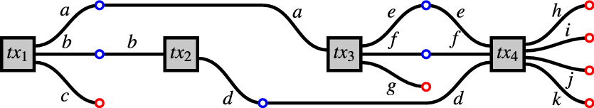
Figure 5. A blockchain
 $\mathcal B=[{tx}_1,{tx}_2,{tx}_3,{tx}_4]$
.
$\mathcal B=[{tx}_1,{tx}_2,{tx}_3,{tx}_4]$
.
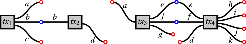
Figure 6.
 $\mathcal B$
chopped up as a blockchain
$\mathcal B$
chopped up as a blockchain
 $[{tx}_1,{tx}_2]$
and a chunk
$[{tx}_1,{tx}_2]$
and a chunk
 $[{tx}_3,{tx}_4]$
.
$[{tx}_3,{tx}_4]$
.
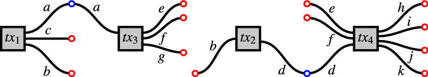
Figure 7.
 $\mathcal B$
chopped up as a blockchain
$\mathcal B$
chopped up as a blockchain
 $[{tx}_1,{tx}_3]$
and a chunk
$[{tx}_1,{tx}_3]$
and a chunk
 $[{tx}_2,{tx}_4]$
.
$[{tx}_2,{tx}_4]$
.
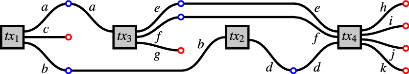
Figure 8. The blockchain
 $\mathcal B'=[{tx}_1,{tx}_3,{tx}_2,{tx}_4]$
.
$\mathcal B'=[{tx}_1,{tx}_3,{tx}_2,{tx}_4]$
.
In the Figures, a blue circle denotes a validator on an output at some position (
 $a,b,c,\dots$
) that has accepted an input and connected to it, and a red circle denotes an unspent input or output, meaning one that has not connected up with a validator to form a spent output-input pair:
$a,b,c,\dots$
) that has accepted an input and connected to it, and a red circle denotes an unspent input or output, meaning one that has not connected up with a validator to form a spent output-input pair:
-
(1).
$\mathcal B$
,
$\mathcal B'$
,
$[{tx}_1,{tx}_2]$
and
$[{tx}_1,{tx}_3]$
are blockchains, because they have unspent outputs (in red) but no unspent inputs. In these blockchains,
${tx}_1$
is what is called the genesis block, meaning the first block in the chain. It follows from the definitions that the genesis block has no inputs.
Footnote 21
-
(2).
$[{tx}]$
(Figure 2) and
$[{tx}_1]$
,
$[{tx}_3,{tx}_4]$
and
$[{tx}_2,{tx}_4]$
are chunks, but not blockchains because they have unspent inputs (in red). -
(3).
$[{tx}_2,{tx}_1]$
is neither a blockchain nor chunk, because the b-input of
${tx}_2$
points to the later b-output of
${tx}_1$
. It is just a list of transactions.


We note two alternative characterisation of blockchains (Definition 3.4.10):
Lemma 3.4.12 A chunk is a blockchain when ….
-
(1). …. the ‘at most one’ in Definition 3.4.1(2) is strengthened to ‘precisely one’.
-
(2). …. the function
$i\mapsto{txs}(i)$
(Definition 3.4.1(2)) is a total function on the inputs in
${txs}$
(so that every input points to precisely one output in an earlier transaction).


Remark 3.4.13 We step back to reflect on Definition 3.4.10. This is supposed to be a paper about blockchains; why did it take us this long to get to them? Because they are a special case of something better and more pertinent: chunks.
A blockchain is just a left-closed chunk. There is nothing wrong with blockchains, but mathematically, chunks seem more interesting:
-
(1). A sublist of a blockchain is a chunk, not a blockchain (we prove this in a moment, in Corollary 3.5.2).
-
(2). A composition of blockchains is possible, but uninteresting, whereas composition of chunks is clearly an interesting operation. Footnote 22
-
(3). If we cut a blockchain into n pieces then we get one blockchain (the initial segment) …. and
$n-1$
chunks. -
(4). Chunks can in any case be viewed as a natural generalisation of blockchains, to allow UTxIs as well as UTxOs.

Definitions and results like Definition 3.5.3, Theorem 3.5.4 and Lemma 3.5.9 inhabit a universe of chunks, not blockchains.
Even in implementation, where we care about real blockchains on real systems, a lot of development work goes into allowing users in practice to download only partial histories of the blockchain rather than having to download and store a complete record – the motivation here is practical, not mathematical – and in the terminology of this paper, we would say that for efficiency we may prefer to work with chunks where possible, because they can be partial and so can be more lightweight.
So the focus of this paper is on chunks: they generalise blockchains, have better mathematical structure, and chunks are in any case where we arrive even if we start off asserting (de)compositional properties of blockchains, and finally – though this is not rigorously explored in this paper, but we would suggest that – chunks are also where we arrive when we consider space-efficient blockchain implementations.
Finally, we mention that blockchains have a right monoid action given by concatenating chunks. Thus, by analogy here with rings and modules, we could imagine for future work a mathematics of blockchains generalising Definition 4.10 such that a ‘blockchain set’ is just any set with a suitable chunk action.
3.5 Properties of chunks and blockchains
3.5.1 Algebraic and closure properties of chunks
Lemma 3.5.1 expresses that a list of transactions is a valid chunk if and only if every sublist of it of length at most two is a valid chunk. In this sense, (in)validity is a local phenomenon:
Lemma 3.5.1 Suppose
 $\mathbb T=(\alpha_{\mathbb T},\beta_{\mathbb T},\textsf{Transaction}_{\mathbb T},\textsf{Validator}_{\mathbb T})$
is an IEUTxO model, and suppose
$\mathbb T=(\alpha_{\mathbb T},\beta_{\mathbb T},\textsf{Transaction}_{\mathbb T},\textsf{Validator}_{\mathbb T})$
is an IEUTxO model, and suppose
 $[{tx}_1,\dots,{tx}_n]\in[\textsf{Transaction}]$
. Then the following conditions are equivalent:
$[{tx}_1,\dots,{tx}_n]\in[\textsf{Transaction}]$
. Then the following conditions are equivalent:
-
•
$[{tx}_i,{tx}_j]\in\textsf{Chunk}$
for every
$1\leq i< j\leq n$
Footnote 23 -
•
$[{tx}_1,\dots,{tx}_n]\in\textsf{Chunk}$


Proof. We note of the well-formedness conditions on chunks from Definition 3.4.1 that they all concern relationships involving at most two transactions.
Corollary 3.5.2
((Validity is down-closed)) Suppose we have an IEUTxO model
 $\mathbb T=(\alpha,\beta,\textsf{Transaction},\textsf{Validator})$
and
$\mathbb T=(\alpha,\beta,\textsf{Transaction},\textsf{Validator})$
and
 $l,l'\in[\textsf{Transaction}]$
.
$l,l'\in[\textsf{Transaction}]$
.
Recall from Notation 2.2.3 that we order lists by sublist inclusion, so
 $l'\leq l$
when l’ is a sublist of l. Then
$l'\leq l$
when l’ is a sublist of l. Then
 \begin{align*}{ch}\in\textsf{Chunk}\ \land\ l'\in[\textsf{Transaction}]\ \land\ l'\leq {ch}\quad\text{implies}\quad l'\in\textsf{Chunk} .\end{align*}
In words: every sublist of a chunk, is itself a chunk.
Proof. From Lemma 3.5.1.
We can wrap up Corollary 3.5.2 in a nice mathematical package:
Definition 3.5.3 Suppose
 $(X,\leq,\bullet,\textsf{e})$
has the following structure:
$(X,\leq,\bullet,\textsf{e})$
has the following structure:
-
(1). X is a set.
-
(2).
$(X,\leq)$
is a partial order, for which
$\textsf{e}$
is a bottom element. -
(3).
$\bullet$
is a partial monoid action on X, meaning that
$(x\bullet y)\bullet z$
exists if and only if
$x\bullet (y\bullet z)$
exists, and if both exist then they are equal.Footnote 24 -
(4).
$\bullet$
is down-closed, meaning that if
$x'\leq x$
and
$x\bullet y$
exists, then so does
$x'\bullet y$
, and similarly for
$y\bullet x$
and
$y\bullet x'$
. -
(5).
$\bullet$
is monotone where defined, meaning that if
$x'\leq x$
then
$x'\bullet y\leq x\bullet y$
(provided
$x\bullet y$
exists), and similarly for
$y\bullet x$
and
$y\bullet x'$
. In this case, call
$(X,\leq,\bullet,\textsf{e})$
a partially ordered partial monoid.


Theorem 3.5.4 Suppose
 $\mathbb T$
is an IEUTxO model (Definition 3.1.9).
$\mathbb T$
is an IEUTxO model (Definition 3.1.9).
Then, its set of chunks
 $\textsf{Chunk}_{\mathbb T}$
(Definition 3.4.1) forms a partially ordered partial monoid (Definition 3.5.3), where
$\textsf{Chunk}_{\mathbb T}$
(Definition 3.4.1) forms a partially ordered partial monoid (Definition 3.5.3), where
-
•
$\leq$
is sublist inclusion, -
•
$\bullet$
is list concatenation, and -
• the unit element is [] the empty set.


Proof. By facts of lists, and Corollary 3.5.2.
3.5.2 Some observations on observational equivalence
Remark 3.5.5 Lemmas 3.5.6 and 3.5.9 apply to IEUTxO models and essentially give criteria for observational equivalence when positions are disjoint.
We find them echoed in the theory of abstract chunk systems as Definitions 4.4.1(5) and 4.4.1(4), and we need them for Proposition 4.4.8.
Lemma 3.5.6 Suppose
 $\mathbb T=(\alpha,\beta,\textsf{Transaction},\textsf{Validator})$
is an IEUTxO model and
$\mathbb T=(\alpha,\beta,\textsf{Transaction},\textsf{Validator})$
is an IEUTxO model and
 ${ch},{ch}'\in\textsf{Chunk}_{\mathbb T}$
. Then
${ch},{ch}'\in\textsf{Chunk}_{\mathbb T}$
. Then
 \begin{align*}{pos}({ch})\cap{pos}({ch}')=\varnothing\quad\text{implies}\quad{ch}\bullet{ch}'\in\textsf{Chunk}_{\mathbb T}.\end{align*}
Proof. By routine checking of possibilities, using the fact that if
 ${pos}({ch})\cap{pos}({ch}')=\varnothing$
(Definition 3.2.3) then they have no positions in common, so no output in one can be called on to validate an input in the other.
${pos}({ch})\cap{pos}({ch}')=\varnothing$
(Definition 3.2.3) then they have no positions in common, so no output in one can be called on to validate an input in the other.
Definition 3.5.7 Suppose
 ${ch},{ch}'\in\textsf{Chunk}_{\mathbb T}$
. Then call
${ch},{ch}'\in\textsf{Chunk}_{\mathbb T}$
. Then call
 ${ch}$
and
${ch}$
and
 ${ch}'$
commuting when
${ch}'$
commuting when
 \begin{align*}\begin{array}{l}{ch}\bullet{ch}'\in\textsf{Chunk}_{\mathbb T}\Longleftrightarrow{ch}'\bullet{ch}\in\textsf{Chunk}_{\mathbb T} .\end{array}\end{align*}
Remark 3.5.8 Definition 3.5.7 is clearly a notion of observational equivalence between
 ${ch}\bullet{ch}'$
and
${ch}\bullet{ch}'$
and
 ${ch}'\bullet{ch}$
where the observable is ‘forms a valid chunk with’. This observable does not depend on internal structure, so we will develop it further once we have abstract chunk systems; see Definition 4.3.16.
${ch}'\bullet{ch}$
where the observable is ‘forms a valid chunk with’. This observable does not depend on internal structure, so we will develop it further once we have abstract chunk systems; see Definition 4.3.16.
For now, Definition 3.5.7 gives us just enough of the background theory of observational equivalence, to state and prove Lemma 3.5.9, Proposition 3.5.12, and Theorem 3.6.1.
Lemma 3.5.9 Suppose
 $\mathbb T=(\alpha,\beta,\textsf{Transaction},\textsf{Validator})$
is an IEUTxO model. Then:
$\mathbb T=(\alpha,\beta,\textsf{Transaction},\textsf{Validator})$
is an IEUTxO model. Then:
-
(1). If
${tx},{tx}'\in\textsf{Transaction}$
and
${pos}({tx})\cap{pos}({tx}')=\varnothing$
(Definition 3. 2.3) then the following all hold:
$$[tx,t{x^\prime }] \in {\rm{Chunk}}\; \Leftrightarrow [t{x^\prime },tx] \in {\rm{Chunk}}\; \Leftrightarrow [tx],[t{x^\prime }] \in {\rm{Chunk}}$$
-
(2). As a corollary, if
${ch},{ch}'\in\textsf{Chunk}$
and
${pos}({ch})\cap{pos}({ch}')=\varnothing$
then
${ch}$
and
${ch}'$
are commuting (Definition 3.5.7).


Proof.
-
(1). By routine checking of possibilities, using the fact that if
${pos}({tx})\cap{pos}({tx}')=\varnothing$
then they have no positions in common, so no output in one can be called upon to validate an input in the other. -
(2). It is a fact that if
${tx}\in l$
then
${pos}({tx})\subseteq{pos}(l)$
and similarly for
${tx}'\in l'$
. The corollary now follows by a routine argument from part 1 of this result and Lemma 3.5.1.


3.5.3 Properties of UTxOs and UTxIs
We return to Definition 3.4.8: Lemma 3.5.10 uses Definition 3.4.8 to note some simple properties of Definition 3.4.1.
Lemma 3.5.10 Suppose
 $\mathbb T$
is an IEUTxO model and
$\mathbb T$
is an IEUTxO model and
 ${ch},{ch}'\in\textsf{Chunk}_{\mathbb T}$
Then:
${ch},{ch}'\in\textsf{Chunk}_{\mathbb T}$
Then:
-
(1).
${utxi}({ch})\cap{utxo}({ch})=\varnothing$
-
(2). If
${ch}\bullet{ch}'\in\textsf{Chunk}_{\mathbb T}$
then
${pos}({ch})\cap{pos}({ch}')\subseteq{utxo}({ch})\cap{utxi}({ch}')$
. -
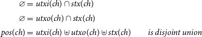
(3).
$\eqalign{
& \emptyset = utxi(ch) \cap stx(ch) \cr
& \emptyset = utxo(ch) \cap stx(ch) \cr
& pos(ch) = utxi(ch) \uplus utxo(ch) \uplus stx(ch)\,\,\,is{\rm{ }}disjo{\mathop{\rm int}} {\rm{ }}union \cr} $


Proof.
-
(1). An input cannot point to a later output, because of Definition 3.4.1(3), and if it points to an earlier output then by construction in Definition 3.4.8 this position no longer labels a UTxO or UTxI. Furthermore a position can be used at most once in an input-output pair, by Definition 3.4.1(2).
-
(2). From Definition 3.4.1(3), as for the previous case.
-
(3). All facts of Definition 3.4.8 and Figure 4.
Remark 3.5.11 Proposition 3.5.12 can be viewed as a stronger version of Lemma 3.5.6. It is an important result because it relates the following apparently different observables:
-
(1). A statically observable property, that
${ch}$
and
${ch}'$
mention disjoint sets of positions. -
(2). A locally observable property, that
${ch}$
and
${ch}'$
compose in both directions. -
(3). An abstract global observable, that
${ch}\bullet{ch}'$
and
${ch}'\bullet{ch}$
can be commuted in any larger chunk.


Compare also with Proposition 4.4.8, which is a similar result but for the differently-constructed abstract chunk systems.
Proposition 3.5.12 Suppose
 $\mathbb T=(\alpha,\beta,\textsf{Transaction},\textsf{Validator})$
is an IEUTxO model and
$\mathbb T=(\alpha,\beta,\textsf{Transaction},\textsf{Validator})$
is an IEUTxO model and
 ${ch},{ch}'\in\textsf{Chunk}_{\mathbb T}$
. Then the following are equivalent:
${ch},{ch}'\in\textsf{Chunk}_{\mathbb T}$
. Then the following are equivalent:
-
(1).
${pos}({ch})\cap{pos}({ch}')=\varnothing$
-
(2).
${ch}\bullet{ch}'\in\textsf{Chunk}_{\mathbb T} \land {ch}'\bullet{ch}\in\textsf{Chunk}_{\mathbb T}$
. -
(3).
${ch}$
and
${ch}'$
are commuting.


Proof. The top-to-bottom implication is Lemma 3.5.6.
For the bottom-to-top implication, suppose that
 ${ch}\bullet{ch}',{ch}'\bullet{ch}\in\textsf{Chunk}_{\mathbb T}$
. From Lemma 3.5.10(2) we have
${ch}\bullet{ch}',{ch}'\bullet{ch}\in\textsf{Chunk}_{\mathbb T}$
. From Lemma 3.5.10(2) we have
 \begin{align*}{pos}({ch})\cap{pos}({ch}')\subseteq ({utxo}({ch})\cap{utxi}({ch}'))\cap({utxo}({ch}')\cap{utxi}({ch})) .\end{align*}
We can rearrange this:
 \begin{align*}{pos}({ch})\cap{pos}({ch}')\subseteq({utxi}({ch})\cap{utxo}({ch}))\cap({utxi}({ch}')\cap{utxo}({ch}')) .\end{align*}
Now we use Lemma 3.5.10(1).
The final part is direct from Lemma 3.5.9(2).
Remark 3.5.13 Proposition 3.5.12 is a resource separation result: if two chunks depend on disjoint resources (disjoint sets of positions) then they commute. This is in the spirit of separation logic (Reynolds 2002), which is a family of logics for reasoning about programs with resource separation in programs – intuitively, that if two programs depend on disjoint resources (e.g. channels or pointers), then they should not interfere with one another, just as we see in Proposition 3.5.12.
It is also in the spirit of a short paper Nester (Reference Nester2021) (which appeared after this paper went into initial review) which uses monoidal categories to reason on resources in a broadly similar spirit, albeit using different methods. A quote from that paper makes a related point: We have seen how the resource theoretic interpretation of monoidal categories, and in particular their string diagrams, captures the sort of material history that concerns ledger structures for blockchain systems. More on this in the Conclusions.
We conclude with Lemma 3.5.14, which we will need later in Lemma 5.2.1:
Lemma 3.5.14 Suppose
 $\mathbb T\in\textsf{IEUTxO}$
is an IEUTxO model and
$\mathbb T\in\textsf{IEUTxO}$
is an IEUTxO model and
 $\pi\in{Perm}$
is a permutation of atoms and
$\pi\in{Perm}$
is a permutation of atoms and
 ${txs}\in[\textsf{Transaction}_{\mathbb T}]$
. Then:
${txs}\in[\textsf{Transaction}_{\mathbb T}]$
. Then:
 \begin{align*}\begin{array}[t]{r@{\ }l}f(\pi{\cdot}{txs}) =&\pi{\cdot} f({txs})\\=& \{\pi(a)\mid a\in f({txs})\}\end{array}\quad\text{for}\ f\in\{{utxi},{utxo},{stx},{pos}\}\end{align*}
In the terminology of Definition 2.3.5:
 ${utxi}$
,
${utxi}$
,
 ${utxo}$
,
${utxo}$
,
 ${stx}$
, and
${stx}$
, and
 ${pos}$
are all equivariant.
${pos}$
are all equivariant.
Proof. Direct from Figure 4 and Definitions 3.4.8 and 2.3.3.
3.6 An application: UTxO systems are ‘Church-Rosser’, in a suitable sense
We now come to Theorem 3.6.1 which is an application of our machinery so far:
Theorem 3.6.1
(Church-Rosser for UTxO) Suppose
 $\mathbb T\in\textsf{IEUTxO}$
and
$\mathbb T\in\textsf{IEUTxO}$
and
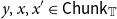 $y,x,x'\in\textsf{Chunk}_{\mathbb T}$
. Suppose further that
$y,x,x'\in\textsf{Chunk}_{\mathbb T}$
. Suppose further that
 \begin{align*}y\bullet x\bullet x'\in\textsf{Chunk}_{\mathbb T}\quad\text{and}\quad{utxi}(y\bullet x') = {utxi}(y\bullet x\bullet x') .\end{align*}
Then we have that:
-
(1). x and x’ are commuting (Definition 3.5.7).
-
(2).
$y\bullet x'\bullet x\in\textsf{Chunk}_{\mathbb T}$
.

Proof. We know by Corollary 3.5.2 (because
 $y\bullet x\bullet x'$
is a chunk) that
$y\bullet x\bullet x'$
is a chunk) that
 $x\bullet x'$
is a chunk, so
$x\bullet x'$
is a chunk, so
 ${pos}(x)\cap{pos}(x')\subseteq{utxo}(x)\cap{utxi}(x')$
.
${pos}(x)\cap{pos}(x')\subseteq{utxo}(x)\cap{utxi}(x')$
.
We also know that
 ${utxi}(y\bullet x')={utxi}(y\bullet x\bullet x')$
and it follows from Definition 3.4.8 that (
${utxi}(y\bullet x')={utxi}(y\bullet x\bullet x')$
and it follows from Definition 3.4.8 that (
 ${utxo}(y)\cap{utxi}(x)=\varnothing$
and)
${utxo}(y)\cap{utxi}(x)=\varnothing$
and)
 ${utxo}(x)\cap{utxi}(x')=\varnothing$
.
Footnote 25
${utxo}(x)\cap{utxi}(x')=\varnothing$
.
Footnote 25
Therefore,
 ${pos}(x)\cap{pos}(x')=\varnothing$
. By Proposition 3.5.12, x and x’ are commuting, and it follows (since
${pos}(x)\cap{pos}(x')=\varnothing$
. By Proposition 3.5.12, x and x’ are commuting, and it follows (since
 $y\bullet x'\bullet x\in\textsf{Chunk}_{\mathbb T}$
) that
$y\bullet x'\bullet x\in\textsf{Chunk}_{\mathbb T}$
) that
 $y\bullet x\bullet x'\in\textsf{Chunk}_{\mathbb T}$
.
$y\bullet x\bullet x'\in\textsf{Chunk}_{\mathbb T}$
.
Recall the definition of a blockchain (Definition 3.4.10) as being a chunk with empty
 ${utxi}$
. Then, we can specialise Theorem 3.6.1 as follows:
${utxi}$
. Then, we can specialise Theorem 3.6.1 as follows:
Corollary 3.6.2 Suppose
 $\mathbb T\in\textsf{IEUTxO}$
and
$\mathbb T\in\textsf{IEUTxO}$
and
 $y,x,x'\in\textsf{Chunk}_{\mathbb T}$
and suppose
$y,x,x'\in\textsf{Chunk}_{\mathbb T}$
and suppose
 $y\bullet x'$
is a blockchain. Then:
$y\bullet x'$
is a blockchain. Then:
-
(1). If
$y\bullet x\bullet x'$
is a blockchain then x and x’ commute. -
(2). If x and x’ do not commute then
$y\bullet x\bullet x'$
is not a blockchain.


Proof. Direct from Theorem 3.6.1, for the case that
 ${utxi}(y\bullet x')={utxi}(y\bullet x\bullet x')=\varnothing$
.
${utxi}(y\bullet x')={utxi}(y\bullet x\bullet x')=\varnothing$
.
Remark 3.6.3 Corollary 3.6.2 models a situation where someone designs a chunk x’ that will successfully attach to a blockchain y, but because this is a distributed system, somebody else gets in and attaches x first.
Then this can only happen if x and x’ are commuting; conversely, if x and x’ are not commuting then one of
 $y\bullet x\bullet x'$
or
$y\bullet x\bullet x'$
or
 $y\bullet x'$
must fail to be a blockchain.
$y\bullet x'$
must fail to be a blockchain.
What makes this interesting is that it is an important correctness property from the point of view of the user who created x’: if x’ is accepted onto both y and
 $y\bullet x$
without failure, then it does not matter that x got in first –
$y\bullet x$
without failure, then it does not matter that x got in first –
 $y\bullet x\bullet x'$
and
$y\bullet x\bullet x'$
and
 $y\bullet x'\bullet x$
are equivalent up to observable behaviour.
$y\bullet x'\bullet x$
are equivalent up to observable behaviour.
Note that:
-
• Theorem 3.6.1 and Corollary 3.6.2 do not state that
$\textsf{IEUTxO}$
systems are insensitive to order, and -
• Theorem 3.6.1 and Corollary 206.2 do not state that all transactions always commute (this is simply not what is written on the page).

Theorem 3.6.1 and Corollary 3.6.2 can be viewed as a purity property, in the sense of functional programming: if x’ successfully combines with y, then inputs to x’ may not be modified by an intervening environment x – there are no side-effects!
More specifically, these results can be viewed as playing a role analogous to a ‘Church-Rosser’ or ‘confluence’ property. To see why, contrast with the situation in an accounts-based system – corresponding to an imperative paradigm – where a transaction may be successfully appended even if parameters to it on the blockchain get modified by intervening transactions.
To take a concrete scenario: I could check my bank account, observe I have enough money for a purchase, submit my transaction – and then go into overdraft and be subject to overdraft fees, because a direct debit happened to arrive in-between (a) my checking my balance and designing my purchase transaction and (b) the payment request for the purchase transaction arriving at my account. This error clearly comes from the use of a stateful, imperative programming style and Theorem 6.1 expresses a rigorous sense in which a corresponding phenomenon is impossible in a UTxO style system. Footnote 26
With this comparison in mind, we see that Theorem 6.1 is a purity result: state is local, and composition of chunks succeeds or fails locally.
We can organise our IEUTxO models into a category:
Definition 3.7.1 Let
 $\textsf{IEUTxO}$
be a category such that:
$\textsf{IEUTxO}$
be a category such that:
-
(1). Objects
$\mathbb S,\mathbb T$
are IEUTxO models (Definition 3.1.2). -
(2). An arrow
$f:\mathbb S\to\mathbb T$
is a map such that if
\begin{align*}f:\textsf{Transaction}_{\mathbb S}\to\textsf{Chunk}_{\mathbb T}\end{align*}
${tx},{tx}'\in\textsf{Transaction}_{\mathbb S}$
then (2)Above,
\begin{equation}[{tx},{tx}']\in\textsf{Chunk}_{\mathbb S}\quad\text{implies}\quad f({tx})\bullet f({tx}')\in\textsf{Chunk}_{\mathbb T}.\end{equation}
$\bullet$
denotes monoid composition, which on chunks is list concatenation; see Notation 2.2.3(4).
-
(3). The identity arrow maps
${tx}$
to
$[{tx}]$
. -
(4). Composition of arrows is pointwise, meaning that if
then
\begin{align*}\begin{array}{r@{\ }l@{\qquad}r@{\ }l}f:&\mathbb S\to\mathbb S'&{tx}\in&\textsf{Transaction}_{\mathbb S}\\f':&\mathbb S'\to\mathbb S''&f({tx})=&[{tx}'_1,\dots,{tx}'_n]\end{array}\end{align*}
$f'f :\mathbb S\to\mathbb S''$
is such that We prove this mapping is indeed an arrow – thus, it maps to chunks – in Corollary 3.7.4.
\begin{align*}{tx}\in\textsf{Transaction}_{\mathbb S} \longmapsto f'({tx}'_1)\bullet\ldots\bullet f'({tx}'_n)\in\textsf{Chunk}_{\mathbb S''} .\end{align*}


Lemma 3.7.2 An arrow
 $f:\mathbb S\to\mathbb T$
(Definition 3.7.1(2)) induces a mapping of chunks
$f:\mathbb S\to\mathbb T$
(Definition 3.7.1(2)) induces a mapping of chunks
 $\textsf{Chunk}_{\mathbb S}\to\textsf{Chunk}_{\mathbb T}$
, by acting on the individual transactions and composing the results:
$\textsf{Chunk}_{\mathbb S}\to\textsf{Chunk}_{\mathbb T}$
, by acting on the individual transactions and composing the results:
 \begin{align*}f([{tx}_1,\dots,{tx}_n]) = f({tx}_1)\bullet \ldots\bullet f({tx}_n) .\end{align*}
Proof. The nontrivial part is to check that
-
• if
${ch}=[{tx}_1,\dots,{tx}_n]$
is a valid chunk in
$\textsf{Chunk}_{\mathbb S}$
, -
• then
$f({tx}_1)\bullet\ldots\bullet f({tx}_n)$
is a valid chunk in
$\textsf{Chunk}_{\mathbb T}$
.


This follows by combining condition 2 of Definition 3.7.1 with Lemma 3.5.1 and Corollary 3.5.2.
Corollary 3.7.3 Condition 2 of Definition 3.7.1 is equivalent to either of the following conditions:
-
(1).
$[{tx}_1,\dots,{tx}_n]\in\textsf{Chunk}_{\mathbb S}$
implies
$f({tx}_1)\bullet\ldots f({tx}_n)\in\textsf{Chunk}_{\mathbb T}$
. -
(2). f induces a monoid homomorphism on chunks.


Proof. The equivalence of conditions 1 and 2 above is routine, given that every chunk factors into singletons. Then, condition (2) in part 2 of Definition 3.7.1 is just a special case of condition 1 above, and the reverse implication is Lemma 3.7.2.
Corollary 3.7.4 Composition of arrows as given in Definition 3.7.1(4) is well-defined; that is, the composition
 $f'\,f$
really is a map from transactions to chunks.
$f'\,f$
really is a map from transactions to chunks.
Proof. Continuing the notation of Definition 3.7.1(4), by assumption f maps
 ${tx}\in\textsf{Transaction}_{\mathbb S}$
to some
${tx}\in\textsf{Transaction}_{\mathbb S}$
to some
 $f({tx})\in\textsf{Chunk}_{\mathbb S'}$
, and then by Lemma 3.7.2 the action of f’ maps
$f({tx})\in\textsf{Chunk}_{\mathbb S'}$
, and then by Lemma 3.7.2 the action of f’ maps
 $f({tx})$
to a valid chunk
$f({tx})$
to a valid chunk
 $f'(f({tx}))\in\textsf{Chunk}_{\mathbb S''}$
.
$f'(f({tx}))\in\textsf{Chunk}_{\mathbb S''}$
.
Remark 3.7.5 ((Comment on design)) We briefly discuss the design decisions embedded in Definition 3.7.1:
-
(1). The conditions in Corollary 3.7.3 are more readable than condition (2) of Definition 3.7.1(2), but this comes at the cost of an additional universally quantified parameter n. It is a matter of taste which version we take as primitive: the one in the Definition has fewest parameters and is easiest to check (a higher-level view will be taken later when we develop abstract chunk systems in Section 4).
-
(2). We could relax the condition to allow f to be a partial map. This would exhibit
$\textsf{IEUTxO}$
as a subcategory of a larger category with the same objects but more arrows, and in particular, it would allow chunks in
$\mathbb S$
to cease to be valid when mapped to
$\mathbb T$
– we would still insist that f be a partial monoid homomorphism on chunks, where everything is defined. We did not choose this design for this paper, but it might be useful for future work; for example following an intuition that
$\mathbb S$
is a liberal universe of chunks, and f maps it to a stricter universe
$\mathbb T$
in which additional restrictions are appended to validators. Thus, chunks in the liberal world might cease to be valid in the stricter universe. -
(3). We could also restrict f further so that
$f:\textsf{Transaction}_{\mathbb S}\to\textsf{Transaction}_{\mathbb T}$
. This would yield fewer arrows, and we prefer to allow the flexibility of mapping a single transaction in
$\mathbb S$
to a chunk of transactions in
$\mathbb T,$
following an intuition that
$\mathbb S$
is a coarse-grained representation which f maps into a finely grained representation where something that was considered a single transaction is now a chunk.


3.8 Idealised UTxO
One special case of IEUTxO deserves its own discussion:
Remark 3.8.1 ((Idealised UTxO)) Recall from Figure 1 that validators take as input a pointed transaction:
 \begin{align*}\textsf{Transaction}_!\subseteq {fin}_!(\textsf{Input})\times{fin}(\textsf{Output}) .\end{align*}
Recall also from Notation 2.2.3(2) and that a pointed transaction is a transaction with one distinguished input of that transaction. For convenience, we will call this the input-point of the transaction.
The UTxO model – on which Bitcoin is based – is the special case of EUTxO where validators just examine the input-point. So intuitively, in the UTxO model a validator of an output sees just the input that points to that output, in the sense of Notation 3.1.3, and it does not pay any attention to the transaction in which that input occurs.
We therefore obtain an Idealised UTxO (IUTxO) model from Figure 1 just by changing the line for validators to:
 \begin{align*}\textsf{Validator} \subseteq {pow}(\beta\times\textsf{Input}) .\end{align*}
There is an easy embedding map which we can write 1, taking an IUTxO model to an IEUTxO model, derived from the embedding
 \begin{align*}{pow}(\beta\times\textsf{Input}) \longrightarrow{pow}(\beta\times\textsf{Transaction}_!)\end{align*}
which is itself derived from the projection taking a pointed transaction to its input-point:
 \begin{align*}\textsf{Transaction}_! \longrightarrow\textsf{Input} .\end{align*}
Then we can define a category of IUTxO models such that
-
• objects are IUTxO models, and
-
• arrows are functions exactly as defined in Definition 3.7.1.
Proposition 3.8.2 The mapping
 ${e}$
extends to a categorical embedding
Footnote 27
${e}$
extends to a categorical embedding
Footnote 27
 $\textsf{IUTxO}\to\textsf{IEUTxO}$
.
$\textsf{IUTxO}\to\textsf{IEUTxO}$
.
Proof. Direct from the construction, since an
 $\textsf{IUTxO}$
model is identified with an
$\textsf{IUTxO}$
model is identified with an
 $\textsf{IEUTxO}$
model whose validators ignore the transaction and just look at the input-point.
$\textsf{IEUTxO}$
model whose validators ignore the transaction and just look at the input-point.
Remark 3.8.3 For convenience, we may treat
 $\textsf{IUTxO}$
as a direct subset of
$\textsf{IUTxO}$
as a direct subset of
 $\textsf{IEUTxO}$
– abusing notation we could write
$\textsf{IEUTxO}$
– abusing notation we could write
 $\textsf{IUTxO}\subseteq\textsf{IEUTxO}$
– thus identifying an IUTxO model with an IEUTxO model whose validators only check the input-point of their transaction. Thus for instance, we wrote ‘is identified with’ in Proposition 3.8.2. It will always be clear what is intended and we could always unroll the injections if required.
$\textsf{IUTxO}\subseteq\textsf{IEUTxO}$
– thus identifying an IUTxO model with an IEUTxO model whose validators only check the input-point of their transaction. Thus for instance, we wrote ‘is identified with’ in Proposition 3.8.2. It will always be clear what is intended and we could always unroll the injections if required.
4. Abstract Chunk Systems:
$\textsf{ACS}$

4.1 Basic definitions
Remark 4.1.1 IEUTxO models are good, because they abstract key features of blockchain architectures in a simple and (I would argue) clear manner: output, input and (valid) combination of transactions to form chunks and then blockchains.
However, IEUTxOs are concrete. An IEUTxO model is full of internal structure, by its very construction as a solution to type equations in Figure 1. We will now set about developing an axiomatic, algebraic account of the essential features that make IEUTxOs interesting.
We recall some basic definitions:
Definition 4.1.2 Suppose
 $\textsf X$
is a set and
$\textsf X$
is a set and
 ${\leq}\subseteq\textsf X^2$
is a relation on
${\leq}\subseteq\textsf X^2$
is a relation on
 $\textsf X$
. Call
$\textsf X$
. Call
 $(\textsf X,\leq)$
a well-ordering when:
$(\textsf X,\leq)$
a well-ordering when:
-
(1).
$\leq$
is a partial order (reflexive, transitive, anti-symmetric), and -
(2).
$\leq$
is well-founded (every descending chain is eventually stationary).
Footnote 28
As per Notation 3.1.5,
$\textsf X$
and
$\leq$
are also assumed equivariant.


Example 3.1.3 This should be familiar, but we give examples:
-
•
$(\mathbb Z,\leq)$
is not well-founded. -
•
$({pow}({\mathbb A}),\subseteq)$
and
$({fin}({\mathbb A}),\subseteq)$
are well-founded. -
•
$[\mathbb N]$
(lists of numbers) with sublist inclusion is well-founded.


Definition 4.1.4 Suppose
 $(\textsf X,\textsf{e},\textsf{f},\leq)$
is a partial order with an equivariant least element
$(\textsf X,\textsf{e},\textsf{f},\leq)$
is a partial order with an equivariant least element
 $\textsf{e}$
and an equivariant greatest element
$\textsf{e}$
and an equivariant greatest element
 $\textsf{f}$
. Call
$\textsf{f}$
. Call
 $x\in \textsf X$
atomic when
$x\in \textsf X$
atomic when
-
(1).
$\textsf{e}\lneq x\lneq \textsf{f}$
and -
(2). for every
$x'\in\textsf X$
if
$x'\leq x$
then either
$x'=\textsf{e}$
or
$x'=x$
. Write
${atomic}(\textsf X)$
for the set of atomic elements of
$\textsf X$
(see also Definition 4.2.5).


If we call
 $x\in\textsf X$
proper when it is neither
$x\in\textsf X$
proper when it is neither
 $\textsf{e}$
nor
$\textsf{e}$
nor
 $\textsf{f}$
(following the standard terminology of proper subset), then an atomic element is “a minimal proper element”.
$\textsf{f}$
(following the standard terminology of proper subset), then an atomic element is “a minimal proper element”.
Remark 4.1.5 The set of atomic elements
 ${atomic}(\textsf X)$
is not to be confused with the set of atoms
${atomic}(\textsf X)$
is not to be confused with the set of atoms
 ${\mathbb A}$
from Definition 2.2.1. This name collision is just a coincidence.
${\mathbb A}$
from Definition 2.2.1. This name collision is just a coincidence.
Lemma 4.1.6 will be useful later:
Lemma 4.1.6 Suppose
 $\mathbb T\in\textsf{IEUTxO}$
and consider
$\mathbb T\in\textsf{IEUTxO}$
and consider
 $\textsf{Chunk}_{\mathbb T}$
(valid lists of transactions; see Definition 3.4.1) as a partial order under sublist inclusion
$\textsf{Chunk}_{\mathbb T}$
(valid lists of transactions; see Definition 3.4.1) as a partial order under sublist inclusion
 $\leq$
.
$\leq$
.
Then the atomic elements in
 $(\textsf{Chunk}_{\mathbb T},\leq)$
are precisely the singleton chunks (Notation 3.4.3).
$(\textsf{Chunk}_{\mathbb T},\leq)$
are precisely the singleton chunks (Notation 3.4.3).
Proof. Using Corollary 3.5.2.
4.2 Monoid of chunks
Definition 4.2.1 Assume we have equivariant data
 $(\textsf X,\textsf{e},\textsf{f},\leq,\bullet)$
where:
$(\textsf X,\textsf{e},\textsf{f},\leq,\bullet)$
where:
-
•
$\textsf X$
is a set. -
•
$\textsf{e},\textsf{f}\in\textsf X$
are called unit and fail respectively. -
•
${\leq} \subseteq\textsf X^2$
is a relation. -
•
$\bullet : \textsf X^2\to\textsf X$
is a composition.


Call
 $(\textsf X,\textsf{e},\textsf{f},\leq,\bullet)$
a monoid of chunks when:
$(\textsf X,\textsf{e},\textsf{f},\leq,\bullet)$
a monoid of chunks when:
-
(1).
$\textsf{e}\bullet x=x=x\bullet \textsf{e}$
. -
(2).
$\textsf{f}\bullet x=\textsf{f}=x\bullet\textsf{f}$
. -
(3).
$\leq$
is a well-ordering for which the unit
$\textsf{e}$
is a bottom element and the paradoxical element
$\textsf{f}$
is a top element. -
(4). Composition
$\bullet$
is associative, and monotone in both components, meaning that
\begin{align*}\begin{array}{r@{\ }l@{\quad\text{implies}\quad}r@{\ }l}x'\leq& x & x'\bullet y\leq& x\bullet y\quad\text{and}\\y\leq& y' & x\bullet y\leq& x\bullet y'.\end{array}\end{align*}
-
(5). Composition is increasing in the sense that
\begin{align*}x\leq x\bullet y\quad\text{and}\quad y\leq x\bullet y.\end{align*}
-
(6). If
$x_1,\dots,x_n\in\textsf X$
and
$x_1\bullet \ldots\bullet x_n=\textsf{f}$
, then there must exist
$1\leq i< j\leq n$
such that
$x_i\bullet x_j=\textsf{f}$
.


Remark 4.2.2 A few comments on Definition 4.2.1:
-
(1). This is a clearly an abstraction of IEUTxO structure, where
$\bullet$
is chunk composition and
$\leq$
is list inclusion (proof in Proposition 5.1.3). This is the key instance of the axioms that motivates the definition – IEUTxOs have more structure, but monoids of chunks is where we start. See also Example 4.2.6(6). -
(2).
$x\bullet y$
is not necessarily a least upper bound for
$\{x,y\}$
. Take
$X=\{1,2\}$
and
$x=[1]$
and
$y=[2]$
in Example 4.2.6(4) (finite lists with a top element). Then
$x\bullet y$
and
$y\bullet x$
are distinct and incomparable, so both are upper bounds for
$\{x,y\}$
but
$x\bullet y\not\leq y\bullet x$
and
$y\bullet x\not\leq x\bullet y$
. -
(3). We see that condition 6 of Definition 4.2.1 closely resembles Lemma 3.5.1, and indeed, the condition is inspired by that very Lemma. We will use this in Proposition 5.1.3.


Notation 4.2.3 As is standard, we may write
 $\textsf X$
for both a monoid of chunks and its carrier set. See for instance the first line of Definition 4.2.4.
$\textsf X$
for both a monoid of chunks and its carrier set. See for instance the first line of Definition 4.2.4.
Definition 4.2.4 Suppose
 $\textsf X=(\textsf X,\textsf{e},\textsf{f},\leq,\bullet)$
is a monoid of chunks.
$\textsf X=(\textsf X,\textsf{e},\textsf{f},\leq,\bullet)$
is a monoid of chunks.
-
(1). If
$x\in \textsf X$
and
$[x_1,\dots,x_n]\in[{atomic}(\textsf X)]$
is a finite list of atomic elementsFootnote 29 in
$\textsf X$
and
\begin{align*}x = x_1\bullet\ldots\bullet x_n\quad\text{then say that}\quad\text{{x} \textbf{factorises} as $[x_1,\dots,x_n]$.}\end{align*}
-
(2). Say that
$\textsf X$
is generated by its atomic elements when every
$x\in\textsf X\setminus\{\textsf{f}\}$
has a (possibly non-unique) factorisation into atomic elements.


Definition 4.2.5
-
(1). Call a monoid of chunks
$\textsf X=(\textsf X,\textsf{e},\textsf{f},\leq,\bullet)$
atomic when:-
a.
$\textsf X$
is generated as a monoid by its atomic elements (Definition 4.2.4). -
b. There exists a factorisation function
${factor}:\textsf X\setminus\{\textsf{f}\}\to[{atomic}(\textsf X)]$
such that for every
$x,y\in\textsf X\setminus\{\textsf{f}\}$
-
-
i.
${factor}(x)$
factorises x (Definition 4.2.4) and -
ii.
${factor}(x\bullet y)={factor}(x)\bullet{factor}(y)$
(the right-hand
$\bullet$
denotes list concatenation; the left-hand
$\bullet$
is the monoid action in
$\textsf X$
). In other words, we say that
$\textsf X$
is atomic when there is a homomorphism of partially ordered monoids from
$\textsf X\setminus\{\textsf{f}\}$
to the space of possible factorisations of its elements. The relevance of this condition is discussed in Remark 6.4.4. -
(2). Call
$\textsf X$
perfectly atomic when it is atomic and furthermore: -
a. factorisations into atom elements are unique and
-
b. if
$x\leq y<\textsf{f}$
and
$x=x_1\bullet\ldots\bullet x_m$
and
$y=y_1\bullet\ldots\bullet y_n$
then
$[x_1,\dots,x_m]\leq[y_1,\dots,y_n]$
(sublist inclusion). The relevance of this condition is discussed in Proposition 7.3.6.


Example 4.2.6 Suppose X is an equivariant set. Then:
-
1.
${pow}(X)$
forms a monoid of chunks, where
$\textsf{e}=\varnothing$
and
$\textsf{f}=X$
, and
$\leq$
is subset inclusion, and composition
$\bullet$
is sets union. It is atomic if and only if X is finite (recall: factorisations must be finite). We obtain a factorisation function by choosing any order on X, and listing elements of any
$X'\subseteq X$
in order. -
2.
${pow}(X)$
forms a monoid of chunks, where: -
−
$\textsf{e}=\varnothing$
and
$\textsf{f}=X$
. -
−
$\leq$
is subset inclusion. -
−
$x\bullet y=x\cup y$
if
$x\cap y=\varnothing$
, and
$x\bullet y=\textsf{f}$
otherwise. It is atomic if and only if X is finite. -
(3).
${fin}(X)\cup \{X\}$
(finite sets of atoms, with a top element) forms an atomic monoid of chunks, using either of the two definitions above for
${pow}(X)$
. -
(4). Finite lists with a top element
$[X]^\top$
– meaning finite lists of elements from X, plus one extra ‘top’ element
$\top$
– form a perfectly atomic monoid of chunks as follows: -
−
$\textsf{e} = []$
and
$\textsf{f} = \top$
. -
−
$\leq$
is sublist inclusion (Notation 2.2.3(5)) and
$l\leq\textsf{f}$
for every finite list l. -
− Composition
$\bullet$
is list concatenation on lists, and
$x\bullet \textsf{f} = \textsf{f} = \textsf{f}\bullet x$
for any x (list, or
$\textsf{f}$
). -
(5) Finite lists with a top element
$[X]^\top$
form an atomic (but not perfectly atomic) monoid of chunks as above, where
$\leq$
and
$\bullet$
are defined as follows: -
−
$l\leq l'$
holds when l is not a singleton list and l is a sublist of l’.So
$[]\leq [x]$
and
$[]\leq [x,z]\leq [x,y,z]$
but
$[x]\not\leq [x,y]$
; and the proper atomic elements are singleton and two-element lists. -
−
$[]\bullet l = l\bullet [] = l$
for any list. -
−
$\textsf{f}\bullet x = \textsf{f} = x\bullet\textsf{f}$
for any x. -
− If l and l’ are nonempty lists, then
$l\bullet l'$
is
$l_{init}$
concatenated with
$l'_{tail}$
, where
$l_{init}$
is everything except for the last element of l, and
$l'_{tail}$
is everything except for the first element of l’. -
(6) As touched on above, if
$\mathbb T$
is an IEUTxO model then
$\mathbb T$
gives rise to a perfectly atomic monoid of chunks. See Proposition 5.1.3.


Remark 4.2.7 It might seem counterintuitive to make failure
 $\textsf{f}$
a top element in Definition 4.2.1, especially if we are used to seeing domain models where ‘failure’ is intuitively ‘non-termination’ and features
$\textsf{f}$
a top element in Definition 4.2.1, especially if we are used to seeing domain models where ‘failure’ is intuitively ‘non-termination’ and features
 $\bot$
as a bottom element.
$\bot$
as a bottom element.
We have a concrete reason for this: our canonical IEUTxO models are based on lists ordered by sublist inclusion, so bottom is already occupied by the empty list [] which plays the role of
 $\textsf{e}$
(see Definition 5.1.1).
$\textsf{e}$
(see Definition 5.1.1).
But also we have abstract justifications: if we think of a chunk system as a many-valued logic (in which truth-values are chunks or blockchains and
 $\leq$
reflects how they accumulate transactions over time), then to exhibit a
$\leq$
reflects how they accumulate transactions over time), then to exhibit a
 $\top$
is to fail to exhibit a concrete witness. Or (thinking perhaps of callCC Clinger et al. Reference Clinger, Friedman and Wand1986) we can think of
$\top$
is to fail to exhibit a concrete witness. Or (thinking perhaps of callCC Clinger et al. Reference Clinger, Friedman and Wand1986) we can think of
 $\textsf{f}$
as a ‘final’ or ‘escape’ element.
$\textsf{f}$
as a ‘final’ or ‘escape’ element.
4.3 Behaviour, positions and equivalence
4.3.1 Left and right behaviour
Definition 4.3.1 Suppose
 $\textsf X=(\textsf X,\textsf{e},\textsf{f},\leq,\bullet)$
is a monoid of chunks. Then we have natural left- and right-behaviour functions:
$\textsf X=(\textsf X,\textsf{e},\textsf{f},\leq,\bullet)$
is a monoid of chunks. Then we have natural left- and right-behaviour functions:
 \begin{align*}\begin{array}{l@{\ }c@{\ }l@{\qquad}l@{\ }c@{\ }l}{leftB}:\textsf X&\to& {pow}(\textsf X)&{rightB}:\textsf X&\to& {pow}(\textsf X)\\{leftB}: x &\mapsto&\{y{\in}\textsf X \mid y\bullet x<\textsf{f}\}&{rightB}:x &\mapsto&\{y{\in}\textsf X \mid x\bullet y<\textsf{f}\}\end{array}\end{align*}
Lemma 4.3.2 Suppose
 $\textsf X$
is a monoid of chunks. Then we have:
$\textsf X$
is a monoid of chunks. Then we have:
-
(1).
${leftB}(\textsf{e})={rightB}(\textsf{e})=\textsf X\setminus\{\textsf{f}\}$
. -
(2).
${leftB}(\textsf{f})={rightB}(\textsf{f})=\varnothing$
.

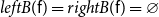
Proof. A fact of Definition 4.2.1(1&2).
Remark 4.3.3 If we think of
 $\textsf{f}$
as a failure element, and we think of
$\textsf{f}$
as a failure element, and we think of
 $x\bullet y$
as being a composition of which we can observe whether it fails or succeeds, then
$x\bullet y$
as being a composition of which we can observe whether it fails or succeeds, then
-
•
${rightB}$
maps
$x\in\textsf X$
to its right-observational behaviour, and -
•
${leftB}$
maps
$x\in\textsf X$
to its left-observational behaviour.


Remark 4.3.4 Parallels can be made in Definition 3.1 with the
 $\lambda$
-calculus (Barendregt 1984) and the
$\lambda$
-calculus (Barendregt 1984) and the
 $\pi$
-calculus (Milner 1999):
$\pi$
-calculus (Milner 1999):
-
(1). In the
$\lambda$
-calculus, a standard observable is non-termination. Here we are doing something similar, except that (as noted in Remark 4.3.3) instead of failure to terminate (
$\bot$
) we observe failure to compose (
$\textsf{f}$
), and we consider combination both to the left and to the right. Continuing the analogy, in the untyped
$\lambda$
-calculus, the left-behaviour set of a term t would be those s such that st terminates; and the right-behaviour set of t would be those s such that ts terminates. -
(2). The
$\pi$
-calculus has notions of communications across channels, and as noted in Remark 3.4.4, we see a resemblance with communication of an input and output on a position. However there are differences, including: -
a. Validation is not primitive in the
$\pi$
-calculus but it is a core precept here. -
b. Communication in the plain
$\pi$
-calculus (without considering dialects) is non-deterministic – one channel name can be invoked by multiple inputs and outputs – whereas here a key assumption is that every channel name (i.e. position) must have one input and one output – and if not, the chunk collapses to a failure error-state
$\textsf{f}$
(cf. the conditions in Definitions 3.4.1 and 3.4.10). -
c. Name restriction in the
$\pi$
-calculus is not automatic but instead is managed by an explicit restriction term-former. In contrast here, a communicating channel (an output-input pair) automatically closes when used once. We say ‘closed’ and not ‘bound’ because the name remains visible in
${up}$
(see also
${stx}$
in the IEUTxO models); it is just that no further communication may occur along it. We discuss garbage-collecting names in chunks in Subsection 8.2.


Remark 4.3.5 Definitions 4.3.6 and 4.3.9 will build on Definitions 4.2.1 and 4.3.1 to derive a full notion of an observable interface of a monoid element, all derived just from the partiality of composition. We will make good use of this in the rest of the development, for instance Definition 6.2.1 depends on it.
4.3.2 Positions
Definition 4.3.6 Suppose
 $\textsf X$
is a monoid of chunks. Define
$\textsf X$
is a monoid of chunks. Define
 ${posi}(x)\subseteq{\mathbb A}$
the positions of
${posi}(x)\subseteq{\mathbb A}$
the positions of
 $x\in\textsf X$
as follows:
$x\in\textsf X$
as follows:
 \begin{align*}\begin{array}{r@{\ }l}{posi}(\textsf{f}_{\textsf X})=&\varnothing\\{posi}(x)=&\{a\in{\mathbb A} \mid \forall{\pi{\in}{fix}(a)}\pi{\cdot} x\not\in{leftB}(x)\cup{rightB}(x) \}\quad (x\in\textsf X\setminus\{\textsf{f}_{\textsf X}\}).\end{array}\end{align*}
(
 ${fix}(a)$
from Definition 2.3.4.)
${fix}(a)$
from Definition 2.3.4.)
Thus,
 $a\in{posi}(x)$
when
$a\in{posi}(x)$
when
 $x\neq\textsf{f}_{\textsf X}$
and
$x\neq\textsf{f}_{\textsf X}$
and
 $\pi{\cdot} x\not\in{leftB}(x)\cup{rightB}(x)$
, for any
$\pi{\cdot} x\not\in{leftB}(x)\cup{rightB}(x)$
, for any
 $\pi$
such that
$\pi$
such that
 $\pi(a)=a$
.
$\pi(a)=a$
.
Remark 4.3.7 Note that the
 ${\cdot}$
in
${\cdot}$
in
 $\pi{\cdot} x$
in Definition 4.3.6 above refers to the atoms-permutation action from Definition 2.3.2, not to the partial monoid action
$\pi{\cdot} x$
in Definition 4.3.6 above refers to the atoms-permutation action from Definition 2.3.2, not to the partial monoid action
 $\bullet$
from Definition 3.5.3.
$\bullet$
from Definition 3.5.3.
Remark 4.3.8 In words,
 ${posi}(x)$
from Definition 4.3.6 is those atoms such that there is no permutation fixing a such that
${posi}(x)$
from Definition 4.3.6 is those atoms such that there is no permutation fixing a such that
 $\pi{\cdot} x$
can be successfully combined (left or right) with x.
$\pi{\cdot} x$
can be successfully combined (left or right) with x.
What is the intuition here?
The name
 ${posi}$
reminds us of
${posi}$
reminds us of
 ${pos}$
from Definition 3.2.3, though the definitions are quite different. They are indeed related; in fact, they are equal in a sense made formal in Proposition 5.2.2 (see also Lemma 6.3.2(2)).
${pos}$
from Definition 3.2.3, though the definitions are quite different. They are indeed related; in fact, they are equal in a sense made formal in Proposition 5.2.2 (see also Lemma 6.3.2(2)).
We do not have all the machinery in place yet, so it may be helpful to point forwards here and observe that conditions 3 and 4 of Definition 4.4.1 can be read as a way to make name-clash into an observable.
So intuitively, Definition 4.3.6 – once combined with the notion of an oriented monoid from Definition 4.4.1 – can use permutations to observe name-clash: it measures the live communication channels
 $a\in{\mathbb A}$
in an element x by forcing name-clashes between a-channels with
$a\in{\mathbb A}$
in an element x by forcing name-clashes between a-channels with
 $\pi$
-renamed variants
$\pi$
-renamed variants
 $\pi{\cdot} x$
for
$\pi{\cdot} x$
for
 $\pi\in{fix}(a)$
. More details will follow, and see Remark 5.2.3.
$\pi\in{fix}(a)$
. More details will follow, and see Remark 5.2.3.
Definition 4.3.9 Suppose
 $\textsf X=(\textsf X,\textsf{e},\textsf{f},\leq,\bullet)$
is a monoid of chunks, and suppose
$\textsf X=(\textsf X,\textsf{e},\textsf{f},\leq,\bullet)$
is a monoid of chunks, and suppose
 $x\in \textsf X$
and
$x\in \textsf X$
and
 $a\in{\mathbb A}$
.
$a\in{\mathbb A}$
.
-
(1). If
then say that a points left in x. Write
\begin{align*}a\in{posi}(x)\quad\text{and}\quad\exists{y{\in}{leftB}(x)}a\in{posi}(y),\end{align*}
${left}(x)\subseteq{\mathbb A}$
for the set of atoms that point left in x.
-
(2). If
then say that a points right in x. Write
\begin{align*}a\in{posi}(x)\quad\text{and}\quad\exists{y{\in}{rightB}(x)}a\in{posi}(y),\end{align*}
${right}(x)\subseteq{\mathbb A}$
for the set of atoms that point right in x.
-
(3). If a points neither left nor right in a and yet
$a\in{posi}(x)$
, so that then say that a points up in x. Write
\begin{align*}a\in{posi}(x)\quad\text{and}\quad\forall{y{\in}{leftB}(x)\cup{rightB}(x)}a\not\in{posi}(y),\end{align*}
${up}(x)\subseteq{\mathbb A}$
for the set of atoms that point up in x.


Lemma 4.3.10 expresses intuitively that atoms that point ‘up’ in a transaction cannot engage in successful (non-failing) combination; they are ‘stuck interfaces’:
Lemma 4.3.10 Suppose
 $\textsf X$
is a monoid of chunks and
$\textsf X$
is a monoid of chunks and
 $x,y\in\textsf X$
and
$x,y\in\textsf X$
and
 $a\in{up}(x)$
. Then
$a\in{up}(x)$
. Then
 \begin{align*}a\in{posi}(y)\quad\text{implies}\quad x\bullet y=y\bullet x=\textsf{f}.\end{align*}
Proof. Direct from Definition 4.3.9(3).
Remark 4.3.11 The reader who sees similarities between the
 ${left}$
,
${left}$
,
 ${right}$
and
${right}$
and
 ${up}$
of Definition 4.3.9, and the
${up}$
of Definition 4.3.9, and the
 ${utxi}$
,
${utxi}$
,
 ${utxo}$
and
${utxo}$
and
 ${stx}$
of Definition 3.4.8 is right: see Proposition 5.2.2, Lemma 5.3.1, and Proposition 5.5.4.
${stx}$
of Definition 3.4.8 is right: see Proposition 5.2.2, Lemma 5.3.1, and Proposition 5.5.4.
A simple lemma will be helpful:
Lemma 4.3.12 Suppose
 $\textsf X$
is a monoid of chunks and
$\textsf X$
is a monoid of chunks and
 $x\in\textsf X$
. Then:
$x\in\textsf X$
. Then:
 \begin{align*}\begin{array}{r@{\ }l}{up}(x)=&{posi}(x)\setminus({left}(x)\cup{right}(x))\\\varnothing=&{left}(x)\cap{up}(x)\\\varnothing=&{right}(x)\cap{up}(x)\\{posi}(x)=&{left}(x)\cup{right}(x)\cup{up}(x)\end{array}\end{align*}
Proof. This just rephrases clause 3 of Definition 4.3.9.
Remark 4.3.13 Lemmas 4.3.12 and 3.5.10(3) are similar but note that the status of the underlying data types is somewhat different:
-
• A chunk
${ch}\in\textsf{Chunk}$
of an IEUTxO model is full of internal structure, and operations on it are defined in terms of that structure, whereas -
• an element
$x\in\textsf X$
in a monoid of chunks is an abstract entity and we assume nothing about its internal structure.


Thus, a similarity between them has significance: it is a sanity check on our model and indicates that something rather abstract (monoids of chunks) is accurately following the behaviour of something more concrete (IEUTxO models).
Remark 4.3.14 Lemma 4.3.12 expresses that every position in some
 $x\in\textsf X$
(Definition 4.3.6) must point in a direction in
$x\in\textsf X$
(Definition 4.3.6) must point in a direction in
 $\{{left},{right},{up}\}$
, and it cannot point both left and up, or both right and up.
$\{{left},{right},{up}\}$
, and it cannot point both left and up, or both right and up.
Note that Definition 4.3.9 admits a possibility that an atom could point both left and right; this cannot happen in the IEUTxO models (see Lemma 3.5.10(1)). We will exclude this when we introduce the notion of an oriented monoid of chunks; see Corollary 4.4.5.
Lemma 4.3.15
-
(1).
${left}(\textsf{e})={right}(\textsf{e})={up}(\textsf{e})=\varnothing$
. -
(2).
${left}(\textsf{f})={right}(\textsf{f})={up}(\textsf{f})=\varnothing$
. -
(3). As a corollary using Lemma 4.3.12,
${posi}(\textsf{e})={posi}(\textsf{f})=\varnothing$
.Footnote 30


Proof. We check the behaviour of
 $\textsf{e}$
and
$\textsf{e}$
and
 $\textsf{f}$
as specified in Definition 4.2.1 against the definitions of
$\textsf{f}$
as specified in Definition 4.2.1 against the definitions of
 ${left}$
,
${left}$
,
 ${right}$
, and
${right}$
, and
 ${up}$
in Definition 4.3.9 and see that this is true.
${up}$
in Definition 4.3.9 and see that this is true.
4.3.3 Observational equivalence
Definition 4.3.16 Suppose
 $\textsf X$
is a monoid of chunks.
$\textsf X$
is a monoid of chunks.
-
(1). Call x and x’ in
$\textsf X$
observationally equivalent and write
\begin{align*}x\sim x'\quad\text{when}\quad{leftB}(x)={leftB}(x')\land {rightB}(x)={rightB}(x') .\end{align*}
-
(2). Say that x and y commute (up to observational equivalence) when
\begin{align*}x\bullet y\sim y\bullet x .\end{align*}


We start with a simple but useful sanity check:
Lemma 4.3.17 Suppose
 $\textsf X$
is a monoid of chunks and
$\textsf X$
is a monoid of chunks and
 $x,y\in\textsf X$
. Then if x and y commute then
$x,y\in\textsf X$
. Then if x and y commute then
 \begin{align*}x\bullet y<\textsf{f} \Longleftrightarrow y\bullet x<\textsf{f}\quad\text{and}\quad x \bullet y=\textsf{f} \Longleftrightarrow y\bullet x=\textsf{f} .\end{align*}
Proof. We unpack Definitions 4.3.16(1&2) and 4.3.1 and conclude that
 \begin{align*}x\bullet y\bullet\textsf{e} <\textsf{f} \Longleftrightarrow y\bullet x\bullet\textsf{e} <\textsf{f} .\end{align*}
The result follows, since
 $\textsf{e}$
is the unit for
$\textsf{e}$
is the unit for
 $\bullet$
.
$\bullet$
.
Lemma 4.3.18 Suppose
 $\textsf X$
is a monoid of chunks. Then if
$\textsf X$
is a monoid of chunks. Then if
 $x\sim x'$
(Definition 4.3.16) then
$x\sim x'$
(Definition 4.3.16) then
 \begin{align*}{left}(x)={left}(x')\quad\text{and}\quad{right}(x)={right}(x')\quad\text{and}\quad{up}(x)={up}(x').\end{align*}
Proof. A fact of Definitions 4.3.16(1) and 4.3.9.
4.4 Oriented monoids
4.4.1 Definition and properties
Definition 4.4.1 Suppose
 $\textsf X=(\textsf X,\textsf{e},\textsf{f},\leq,\bullet)$
is a monoid of chunks.
$\textsf X=(\textsf X,\textsf{e},\textsf{f},\leq,\bullet)$
is a monoid of chunks.
Call
 $\textsf X$
oriented when for all
$\textsf X$
oriented when for all
 $x,y\in\textsf X$
:
$x,y\in\textsf X$
:
-
(1).
${posi}(x)\mathbin{\subseteq_{\text{\it fin}}}{\mathbb A}$
. -
(2). If
${posi}(x)=\varnothing$
then
$x\in\{\textsf{e},\textsf{f}\}$
. -
(3). If
${left}(x)\cap{right}(y)\neq\varnothing$
then
$x\bullet y=\textsf{f}$
. -
(4). If
${posi}(x)\cap{posi}(y)=\varnothing$
then x and y commute up to observational equivalence (Definition 4.3.16(2)). -
(5). If
${posi}(x)\cap{posi}(y)=\varnothing$
and
$\textsf{f}\not\in\{x,y\}$
then
$x\bullet y<\textsf{f}$
.


Remark 4.4.2 We discuss the conditions of Definition 4.4.1 in turn:
-
(1). An element
$x\in\textsf X$
can only be accessible on finitely many channel interfaces. -
(2). The only elements without any interface (meaning atoms that point left right or up) are the unit element (
$\leq$
-bottom) and the failure element (
$\leq$
-top). Compare with the IEUTxO property Lemma 3.2.5. We use this in Lemmas 4.4.6 and 6.3.1. -
(3). Interfaces always try to connect, but can only successfully connect if the directions of their interfaces match up; if not, the whole combination fails. We use this in Lemma 4.4.6, which is required for Proposition 4.4.8.
-
(4). This condition echoes Lemma 3.5.9(2). We use it in Proposition 4.4.8.
-
(5). Elements with no channels in common, cannot fail to compose.


We will show later that the IEUTxO models from Definition 3.1.9 are models of Definition 4.4.1 in a suitable sense; see Proposition 5.3.3.
We can strengthen Definition 4.4.1(2) to a logical equivalence:
Lemma 4.4.3 Suppose
 $\textsf X$
is an oriented monoid of chunks and
$\textsf X$
is an oriented monoid of chunks and
 $x\in\textsf X$
. Then
$x\in\textsf X$
. Then
 \begin{align*}{posi}(x)=\varnothing\quad\text{if and only if}\quad x\in\{\textsf{e},\textsf{f}\} .\end{align*}
Proof. The right-to-left implication is direct from Definition 4.4.1(2). The left-to-right implication is Lemma 4.3.15.
Lemma 4.4.4 is a nice way to repackage Definition 4.4.1(2) in a slightly more accessible wrapper. In its form it resembles Lemma 4.5.10(2), and we use it for Corollary 4.4.5:
Lemma 4.4.4 Suppose
 $\textsf X$
is an oriented monoid of chunks and suppose
$\textsf X$
is an oriented monoid of chunks and suppose
 $x,y\in\textsf X$
. Then
$x,y\in\textsf X$
. Then
 \begin{align*}x\bullet y<\textsf{f}\quad\text{implies}\quad{posi}(x)\cap{posi}(y)\subseteq{right}(x)\cap{left}(y).\end{align*}
Proof. We consider the possibilities, using Lemma 4.3.12:
-
• Suppose
$a\in{left}(x)\cap{posi}(y)$
. From Definition 4.4.1(3)
$a\not\in{right}(x)$
, and by Lemma 4.3.12
$a\in{posi}(x)$
. It follows from Definition 4.3.9(2) that
$x\bullet y=\textsf{f}$
. -
• Suppose
$a\in{right}(y)\cap{posi}(x)$
. From Definition 4.4.1(3)
$a\not\in{left}(y)$
, and by Lemma 4.3.12
$a\in{posi}(y)$
. It follows from Definition 4.3.9(1) that
$x\bullet y=\textsf{f}$
. -
• Other cases are from Lemma 4.3.10 (or by direct reasoning from Definition 4.3.9(3)).


Corollary 4.4.5 is a slightly magical result, in the sense that it is perhaps not immediately obvious that it should follow from our definitions so far. In its form, if not its proof, it clearly resembles Lemma 3.5.10(1). We need it for Lemma 6.2.5, that atomic elements in
 $\textsf X$
generate valid singleton chunks under a mapping to IEUTxO models F:
$\textsf X$
generate valid singleton chunks under a mapping to IEUTxO models F:
Corollary 4.4.5 Suppose
 $\textsf X$
is an oriented monoid of chunks and
$\textsf X$
is an oriented monoid of chunks and
 $x\in\textsf X$
. Then:Footnote 31
$x\in\textsf X$
. Then:Footnote 31
 \begin{align*}{left}(x)\cap{right}(x)=\varnothing .\end{align*}
Proof. Suppose
 $a\in{left}(x)$
, we will show that
$a\in{left}(x)$
, we will show that
 $a\in{right}(x)$
is impossible. Consider some
$a\in{right}(x)$
is impossible. Consider some
 $y\in\textsf X$
with
$y\in\textsf X$
with
 $a\in{posi}(y)$
, so that by Lemma 4.3.12
$a\in{posi}(y)$
, so that by Lemma 4.3.12
 $a\in{left}(y)\cup{right}(y)\cup{up}(y)$
. Then:
$a\in{left}(y)\cup{right}(y)\cup{up}(y)$
. Then:
-
• If
$a\in{left}(y)$
then
$a\in{left}(x)\cap{left}(y)$
and by Lemma 4.4.4
$x\bullet y=\textsf{f}$
. -
• If
$a\in{right}(y)$
then
$a\in{left}(x)\cap{right}(y)$
and by Lemma 4.4.4
$x\bullet y=\textsf{f}$
. -
• If
$a\in{up}(y)$
then
$a\in{left}(x)\cap{up}(y)$
and by Lemma 4.4.4
$x\bullet y=\textsf{f}$
.


Thus,
 $a\in{posi}(y)$
implies
$a\in{posi}(y)$
implies
 $x\bullet y=\textsf{f}$
and so
$x\bullet y=\textsf{f}$
and so
 $y\not\in{rightB}(x)$
. It follows from Definition 4.3.9(2) that
$y\not\in{rightB}(x)$
. It follows from Definition 4.3.9(2) that
 $a\not\in{right}(x)$
as required.
$a\not\in{right}(x)$
as required.
We use Lemma 4.4.6 for Proposition 4.4.8:
Lemma 4.4.6 Suppose
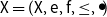 $\textsf X=(\textsf X,\textsf{e},\textsf{f},\leq,\bullet)$
is an oriented monoid of chunks. Then at least one of the following must hold:
$\textsf X=(\textsf X,\textsf{e},\textsf{f},\leq,\bullet)$
is an oriented monoid of chunks. Then at least one of the following must hold:
 \begin{align*}x\bullet y=\textsf{f}\qquad y\bullet x=\textsf{f}\qquad{posi}(x)\cap{posi}(y)=\varnothing\end{align*}
Proof. If x or y are equal to
 $\textsf{e}$
or
$\textsf{e}$
or
 $\textsf{f}$
then
$\textsf{f}$
then
 ${posi}(x)\cap{posi}(y)=\varnothing$
is immediate from Lemma 4.3.
${posi}(x)\cap{posi}(y)=\varnothing$
is immediate from Lemma 4.3.
So suppose
 $x,y\not\in\{\textsf{e},\textsf{f}\}$
, from which it follows by Lemma 4.4.3 (or direct from Definition 4.4.1(2)) that
$x,y\not\in\{\textsf{e},\textsf{f}\}$
, from which it follows by Lemma 4.4.3 (or direct from Definition 4.4.1(2)) that
 ${posi}(x)\neq\varnothing$
and
${posi}(x)\neq\varnothing$
and
 ${posi}(y)\neq\varnothing$
. Suppose we have some
${posi}(y)\neq\varnothing$
. Suppose we have some
 $a\in{posi}(x)\cap{posi}(y)$
. We reason by cases using our assumption that
$a\in{posi}(x)\cap{posi}(y)$
. We reason by cases using our assumption that
 $\textsf X$
is oriented (Definition 4.4.1):
$\textsf X$
is oriented (Definition 4.4.1):
-
• If
$a\in{left}(x)\cap{right}(y)$
then
$x\bullet y=\textsf{f}$
by Definition 4.4.1(3). -
• If
$a\in{right}(x)\cap{left}(y)$
then
$y\bullet x=\textsf{f}$
by Definition 4.4.1(3). -
• If
$a\in{up}(x)$
or
$a\in{up}(y)$
then
$x\bullet y=y\bullet x=\textsf{f}$
by Lemma 4.3.10. -
• Other cases are no harder.


Remark 4.4.7 Proposition 4.4.8 is a partial converse to Definition 4.4.1(4) (compare also with Proposition 3.5.12, which is the same result but for a different structure, and with a very different proof). It is significant because it equates
-
• a static property of positions, with
-
• a local property of being combinable in either order, with
-
• a global operational property of being commutative up to observation. Commutativity is of particular interest in the context of blockchains, because they are by design intended to be distributed, so that we cannot in general know or assume in what order transactions get appended.
Proposition 4.4.8 Suppose
 $\textsf X=(\textsf X,\textsf{e},\textsf{f},\leq,\bullet)$
is an oriented monoid of chunks, and
$\textsf X=(\textsf X,\textsf{e},\textsf{f},\leq,\bullet)$
is an oriented monoid of chunks, and
 $x,y\in\textsf X$
. Suppose further that
$x,y\in\textsf X$
. Suppose further that
 $x\bullet y<\textsf{f}$
or
$x\bullet y<\textsf{f}$
or
 $y\bullet x<\textsf{f}$
(not necessarily both). Then, the following conditions are equivalent:
$y\bullet x<\textsf{f}$
(not necessarily both). Then, the following conditions are equivalent:
-
(1).
${posi}(x)\cap{posi}(y)=\varnothing$
. -
(2).
$x\bullet y<\textsf{f} \land y\bullet x<\textsf{f}$
. -
(3). x and y commute up to observational equivalence (Definition 4.3.16(2)).

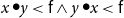
Proof. First, note that since
 $x\bullet y<\textsf{f}$
or
$x\bullet y<\textsf{f}$
or
 $y\bullet x<\textsf{f}$
, it must from Definition 4.2.1(1) be the case that
$y\bullet x<\textsf{f}$
, it must from Definition 4.2.1(1) be the case that
 $x<\textsf{f}$
and
$x<\textsf{f}$
and
 $y<\textsf{f}$
.
$y<\textsf{f}$
.
If
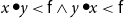 $x\bullet y<\textsf{f}\land y\bullet x<\textsf{f}$
then
$x\bullet y<\textsf{f}\land y\bullet x<\textsf{f}$
then
 ${posi}(x)\cap{posi}(y)=\varnothing$
by Lemma 4.4.6. Conversely if
${posi}(x)\cap{posi}(y)=\varnothing$
by Lemma 4.4.6. Conversely if
 ${posi}(x)\cap{posi}(y)=\varnothing$
then (since
${posi}(x)\cap{posi}(y)=\varnothing$
then (since
 $x<\textsf{f}$
and
$x<\textsf{f}$
and
 $y<\textsf{f}$
) by Definition 4.4.1(5)
$y<\textsf{f}$
) by Definition 4.4.1(5)
 $x\bullet y<\textsf{f}$
and
$x\bullet y<\textsf{f}$
and
 $y\bullet x<\textsf{f}$
.
$y\bullet x<\textsf{f}$
.
If
 ${posi}(x)\cap{posi}(y)=\varnothing$
then x and y commute by Definition 4.4.1(4). Conversely, if
${posi}(x)\cap{posi}(y)=\varnothing$
then x and y commute by Definition 4.4.1(4). Conversely, if
 ${posi}(x)\cap{posi}(y)\neq\varnothing$
then by Lemma 4.4.6 (since
${posi}(x)\cap{posi}(y)\neq\varnothing$
then by Lemma 4.4.6 (since
 $x\bullet y<\textsf{f}$
or
$x\bullet y<\textsf{f}$
or
 $y\bullet x<\textsf{f}$
) we have that
$y\bullet x<\textsf{f}$
) we have that
 $y\bullet x=\textsf{f}$
or
$y\bullet x=\textsf{f}$
or
 $x\bullet y=\textsf{f},$
respectively, and in particular, we have that
$x\bullet y=\textsf{f},$
respectively, and in particular, we have that
 $x\bullet y\neq y\bullet x$
. Using Lemma 4.3.17 we conclude that x and y do not commute.
$x\bullet y\neq y\bullet x$
. Using Lemma 4.3.17 we conclude that x and y do not commute.
Remark 4.4.9 ((Comment on design)) There is design freedom to Definition 4.1, and we mention this briefly for future work. One plausible condition is:
 \begin{align*}{up}(x\bullet y)\subseteq{up}(x)\cup{up}(y)\cup({right}(x)\cap{left}(y)).\end{align*}
Intuitively, this states that combining x and y can only bind positions that point right in x and point left in y. An even stricter variant would be to insist on equality provided that
 $x\bullet y\neq\textsf{f}$
.
$x\bullet y\neq\textsf{f}$
.
4.4.2 A brief discussion
We might ask: Why bother with monoids of chunks? Why not just work with IEUTxOs?
The answer is that we need both: IEUTxOs are the motivating concrete model, and monoids of chunks are their abstraction.
Of course, the IEUTxO equations from Figure 1 themselves are an abstraction and generalisation of a concrete inductive definition in Chakravarty et al. (Reference Chakravarty, Chapman, MacKenzie, Melkonian, Peyton Jones and Wadler2020), Figure 3, so in overview this paper has the following hierarchy of models, given in increasing order of generality –
-
• The inductive EUTxO structures from Chakravarty et al. (Reference Chakravarty, Chapman, MacKenzie, Melkonian, Peyton Jones and Wadler2020).
-
• IEUTxO models from Definition 3.1.2.
-
• Abstract chunk systems (ACS) from Definition 4.5.1.
– though there is also more going on, because we also map from ACS back down to IEUTxO (Theorem 7.3.4 and surrounding discussion).
Programmers can think of APIs, which abstract away from internal structure of a concrete implementation; this makes programs more modular, and easier to test and document.
Modern programming languages make it easier to program efficiently using abstract denotations, instantiating only when needed – one might call this just-in-time instantiation. So even if we have just one concrete model and want one implementation, a good algebraic theory is still relevant to producing working code, because
-
• it may help structure the mathematics and the code – the algebraic graphs with class Haskell package illustrates how effective this marriage of theory and practice can be Mokhov (Reference Mokhov2017) – and
-
• an abstraction can be read as a library of testable properties, against which implementations can be checked. If an implementation fails an axiom – it’s wrong.
So perhaps a better question is this: What are the essential properties of
 $\textsf{IEUTxO}$
that make it interesting? How are these properties layered, and nested; and how can they be compactly represented? Definitions 4.2.1 and 4.4.1 are one set of answers to these questions. And then, a further question is this: What other models, aside from
$\textsf{IEUTxO}$
that make it interesting? How are these properties layered, and nested; and how can they be compactly represented? Definitions 4.2.1 and 4.4.1 are one set of answers to these questions. And then, a further question is this: What other models, aside from
 $\textsf{IEUTxO}$
models, exist of the ACS axioms? This paper contains one answer (plus examples; see Subsection 4.6): in Definitions 6.2.1 and 6.4.1 and Proposition 6.4.3 we give a functor taking any oriented monoid of chunks to IEUTxOs. We also map functorially in the other direction in Definitions 5.1.1 and 5.4.1 and Theorem 5.4.4.
$\textsf{IEUTxO}$
models, exist of the ACS axioms? This paper contains one answer (plus examples; see Subsection 4.6): in Definitions 6.2.1 and 6.4.1 and Proposition 6.4.3 we give a functor taking any oriented monoid of chunks to IEUTxOs. We also map functorially in the other direction in Definitions 5.1.1 and 5.4.1 and Theorem 5.4.4.
The overall results are packaged up in Theorem 7.3.4.
4.5 The category
$\textsf{ACS}$
of abstract chunk systems

We are now ready to give the algebraic account of IEUTxOs promised in Remark 4.1.1: Footnote 32
Definition 4.5.1 An abstract chunk system (ACS) is an oriented atomic monoid of chunks (Definitions 4.4.1, 4.2.5, and 4.2.1).
Definition 4.5.2 Define
 $\textsf{ACS}$
the category of abstract chunk systems by:
$\textsf{ACS}$
the category of abstract chunk systems by:
-
(1). Objects are abstract chunk systems (Definition 4.5.1).
-
(2). Arrows
$g:\textsf X\to\textsf Y$
are sets functions from
$\textsf X$
to
$\textsf Y$
such that:-
a.
$g(\textsf{e}_{\textsf X})=\textsf{e}_{\textsf Y}$
and
$g(\textsf{f}_{\textsf X})=\textsf{f}_{\textsf Y}$
-
b.
$x\leq y<\textsf{f}_{\textsf X}$
implies
$g(x)\leq g(y)<\textsf{f}_{\textsf Y}$
-
c.
$g(x)\bullet g(y)= g(x\bullet y)$
-


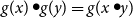
Composition of arrows is composition of functions, and the identity arrow is the identity function.
Remark 4.5.3 ((Comment on design))
-
(1). We do not insist in Definition 4.5.2 that g(x) must be atomic if x is. This corresponds to our choice in Definition 4.7.1(2) to let f map from transactions to chunks, and not from transactions to transactions.
-
(2). We do insist in Definition 4.5.2(2) that if x is not the failure element
$\textsf{f}_{\textsf X}$
in
$\textsf X$
then g(x) is also not the failure element
$\textsf{f}_{\textsf Y}$
in
$\textsf Y$
. This corresponds to our choice in Definition 3.7.1(2) to make f a total function from transactions to chunks, rather than a partial one (cf. discussion in Remark 3.7.5(2)).


We could relax this condition by allowing g to map
 $x<\textsf{f}_{\textsf X}$
to
$x<\textsf{f}_{\textsf X}$
to
 $\textsf{f}_{\textsf Y}$
. There would be nothing wrong with this, and it would just exhibit
$\textsf{f}_{\textsf Y}$
. There would be nothing wrong with this, and it would just exhibit
 $\textsf{ACS}$
as embedded in a larger category with the same objects but more arrows.
$\textsf{ACS}$
as embedded in a larger category with the same objects but more arrows.
Lemma 4.5.4 just repackages Definition 4.2.5 for objects in
 $\textsf{ACS}$
:
$\textsf{ACS}$
:
Lemma 4.5.4 Suppose
 $\textsf X,\textsf Y\in\textsf{ACS}$
and
$\textsf X,\textsf Y\in\textsf{ACS}$
and
 $x\in\textsf X$
and
$x\in\textsf X$
and
 $g:\textsf X\to\textsf Y\in\textsf{ACS}$
. Then:
$g:\textsf X\to\textsf Y\in\textsf{ACS}$
. Then:
-
• If
$x\neq\textsf{f}$
then there exists some finite (possibly empty, possibly non-unique) list of atomic elements
$x_1,\dots,x_n\in {atomic}(\textsf X)$
such that
$x=x_1\bullet\ldots\bullet x_n$
. -
• If
$x\neq\textsf{f}$
(and in particular by Definition 4.1.4(1) if x is atomic) then there exists some finite (possibly empty, possibly non-unique) list of atomic elements
$y_1,\dots,y_n\in {atomic}(\textsf Y)$
such that
$g(x)=y_1\bullet\ldots\bullet y_n$
.


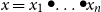

Proof. Immediate since by Definition 4.5.1
 $\textsf X$
is atomic (Definition 4.2.5).
$\textsf X$
is atomic (Definition 4.2.5).
Proposition 4.5.5
-
(1). An arrow
$g:\textsf X\to\textsf Y\in\textsf{ACS}$
(Definition 4.5.2(2)) is uniquely determined by its action on
${atomic}(\textsf X)$
. -
(2). As a corollary, if
$g,g':\textsf X\to\textsf Y$
are two arrows, then to check the equality of arrows
$g=g'$
it suffices to check that
$g(x)=g'(x)$
for every
$x\in{atomic}(\textsf X)$
.


Proof.
-
(1). Consider some
$x\in\textsf X$
. If
$x\in\{\textsf{f},\textsf{e}\}$
then the action of f is determined by Definition 4.5.2(2a).Otherwise, using Lemma 4.5.4 write
$x=x_1\bullet \dots \bullet x_n$
for atomic
$x_1,\dots,x_n\in {atomic}(\textsf X)$
. We then have from Definition 4.5.2(2c) that Thus g(x) is determined by the values of
\begin{align*}f(x_1)\bullet\ldots\bullet g(x_n)= g(x).\end{align*}
$g(x_1)$
, ….,
$g(x_n)$
.
-
(2). By a routine argument from Definition 4.2.5 (since
$\textsf X$
is atomic) and Definition 4.5.2(2c).


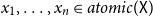


4.6 Examples of abstract chunk systems
We created abstract chunk systems in (Definition 4.5.1) to abstract away the internal structure of IEUTxO models (Definition 3.1.2).
This is a standard move in mathematics: axiomatise, then generalise. As we argued in Subsections 1.1 and 4.4.2, even if the reader only cares about practical hands-on implementation, for which internal structure is available because we have the code, it is still useful – and arguably indispensable – to take a moment to get a good higher-view of what it is that is implemented, since axioms provide a language for the higher-level enterprises of comparison, description, specification, correctness, testing and exposition.
Now we take a moment to go back and consider what the space of concrete models of the ACS axioms looks like. We give a list of examples, which is not intended to be exhaustive but which we hope may illustrate the scope, character, and structure of our definition:
-
(1). Consider the set of all finite sets of atoms
$A=\{a_1,\dots,a_n\}\mathbin{\subseteq_{\text{\it fin}}}\mathbb A$
and
${\mathbb A}$
itself:
\begin{align*}\textsf X={fin}({\mathbb A})\cup\{{\mathbb A}\} .\end{align*}
$\textsf X$
forms an ACS such that
-
−
$A\leq B$
when
$A\subseteq B$
. -
−
$A\bullet B=A\uplus B$
(disjoint union) if A and B are disjoint, and
$A\bullet B=\mathbb A$
otherwise. Unpacking definitions, we can check that: -
− Atomic elements are singletons
$\{a\}$
. -
− A factorisation function
${factor}$
(Definition 4.2.5(1b)) is obtained by ordering atoms and listing the finite set in order. -
−
${posi}(A)={up}(A)=A$
and
${left}(A)={right}(A)=\varnothing$
. -
(2). Consider some data type
$\textsf{Terms}$
of term syntax over variable symbols
$a,b,c,\dots$
(terms of first-order logic
$s,t::= a \mid f(t,\dots,t)$
for some term-formers f, or terms of the untyped
$\lambda$
-calculus
$s,t::=a \mid ss\mid\lambda a.s$
would suffice). Let finite substitutions be finite partial maps from variable symbols to terms generated by atomic substitutions Composition is defined in a standard way by acting on terms as
\begin{align*}\sigma=[a{{:}\text{=}} t] .\end{align*}
$s\sigma$
. If
$a\not\in{dom}(\sigma)$
then
$a\sigma=a$
(so the substitution acts as the identity on variable symbols not in its domain). Now, add a fail top element
$\textsf{f}$
, such that
$s\textsf{f}=s$
always (so
$\textsf{f}$
is a formal element that acts as the identity). If the reader likes, we could take
$\textsf{f}$
to be
$[a{{:}\text{=}} a\mid \text{ all }a]$
. Then substitutions with
$\textsf{f}$
form an ACS, where
-
−
$\sigma\leq\sigma'$
when
${dom}(\sigma)\subseteq{dom}(\sigma')$
, and
$\sigma\leq\textsf{f}$
always. -
− If
${dom}(\sigma)\cap{dom}(\sigma')=\varnothing$
then
$\sigma\bullet\sigma'$
is the finite substitution that maps a to
$a\sigma\sigma'$
for each
$a\in{dom}(\sigma)\cup{dom}(\sigma')$
, and -
− if
${dom}(\sigma)\cap{dom}(\sigma')\neq\varnothing$
then
$\sigma\bullet\sigma'=\textsf{f}$
The ‘disjoint domains or fail’ condition ensures that composition is monotone in
$\leq$
. Unpacking definitions, we check that: -
− Atomic elements are the generators
$[a{{:}\text{=}} s]$
. -
− A factorisation function
${factor}$
(Definition 4.2.5(1b)) is obtained by ordering atoms and listing a substitution as a list of atomic substitutions in order of the atom on the left.Footnote 33 -
−
${posi}(\sigma)={left}(\sigma)={dom}(\sigma)$
and
${right}(\sigma)={up}(\sigma)=\varnothing$
.
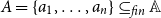


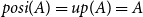
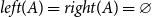


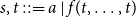

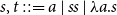


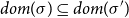

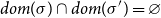


5. The Functor
$F:\textsf{IEUTxO}\to\textsf{ACS}$

5.1 Action on objects
Definition 5.1.1 Suppose
 $\mathbb T=(\alpha,\beta,\textsf{Transaction},\textsf{Validator})\in\textsf{IEUTxO}$
is a model (Definition 3.1.9) and recall
$\mathbb T=(\alpha,\beta,\textsf{Transaction},\textsf{Validator})\in\textsf{IEUTxO}$
is a model (Definition 3.1.9) and recall
 $\textsf{Chunk}_{\mathbb T}$
from Notation 4.3. Then, we define an abstract chunk system
$\textsf{Chunk}_{\mathbb T}$
from Notation 4.3. Then, we define an abstract chunk system
 \begin{align*}F(\mathbb T) = (\textsf{Chunk}_{\mathbb T}\cup\{{fail}\},[],{fail},\leq,\bullet) \in \textsf{ACS}\end{align*}
as follows:
-
• The underlying set is
$\textsf{Chunk}_{\mathbb T}\cup\{{fail}\}$
– so if we write “
$x\in F(\mathbb T)$
” this means “either
$x={fail}$
or
$x\in\textsf{Chunk}_{\mathbb T}$
”. -
•
$\textsf{e}=[]$
and
$\textsf{f}={fail}$
. -
•
$\leq$
is sublist inclusion (Notation 2.2.3(5)) on chunks that are lists of transactions, with
$\textsf{f}$
as a top element, so
${ch}\leq\textsf{f}$
always. -
•
$x\bullet\textsf{f}=\textsf{f}=\textsf{f}\bullet x$
, and if x and y are both chunks then
$\bullet$
is validated concatenation of chunks, defaulting to the failure element
$\textsf{f}$
if validation fails.


Remark 5.1.2 So if
 $x,y\in\textsf{Chunk}_{\mathbb T}$
but
$x,y\in\textsf{Chunk}_{\mathbb T}$
but
 $x\bullet y\in[\textsf{Transaction}_{\mathbb T}]\setminus\textsf{Chunk}_{\mathbb T}$
in
$x\bullet y\in[\textsf{Transaction}_{\mathbb T}]\setminus\textsf{Chunk}_{\mathbb T}$
in
 $\mathbb T$
– so the two chunks cannot be validly combined in
$\mathbb T$
– so the two chunks cannot be validly combined in
 $\mathbb T$
– then
$\mathbb T$
– then
 $x\bullet y={fail}$
in
$x\bullet y={fail}$
in
 $F(\mathbb T)$
. We will always be clear whether
$F(\mathbb T)$
. We will always be clear whether
 $\bullet$
means ‘concatenate as lists’ or ‘compose in
$\bullet$
means ‘concatenate as lists’ or ‘compose in
 $F(\mathbb T)$
’.
$F(\mathbb T)$
’.
 $F(\mathbb T)$
resembles
$F(\mathbb T)$
resembles
 $\mathbb T$
, except with an explicit failure element
$\mathbb T$
, except with an explicit failure element
 ${fail}$
added. This makes monoid composition total: not every pair of chunks composes to form a list of transactions that is a chunk – as per the criteria in Definition 3.4.1 – thus any combination of chunks that is not a chunk, can be set to
${fail}$
added. This makes monoid composition total: not every pair of chunks composes to form a list of transactions that is a chunk – as per the criteria in Definition 3.4.1 – thus any combination of chunks that is not a chunk, can be set to
 ${fail}$
.
${fail}$
.
We still need to prove that
 $F(\mathbb T)$
is an abstract chunk system (Definition 4.5.1) in the category
$F(\mathbb T)$
is an abstract chunk system (Definition 4.5.1) in the category
 $\textsf{ACS}$
(Definition 4.5.2(1)) thus:
$\textsf{ACS}$
(Definition 4.5.2(1)) thus:
-
•
$F(\mathbb T)$
is a monoid of chunks (Definition 4.2.1), -
•
$F(\mathbb T)$
is atomic (Definition 4.2.5) – in fact it is perfectly atomic (Definition 4.2.5(2)) – and -
•
$F(\mathbb T)$
is oriented (Definition 4.4.1).


We do this next, culminating with Theorem 5.3.4.
Note that this gives us a dual view of a chunk:
-
• as a chunk in the IEUTxO universe, and
-
• as an abstract element in the ACS universe.
To what extent do these two views correspond, and how can we make this formal? We prove Proposition 5.2.2, which verifies that the positions in a chunk as an element in the IEUTxO universe, coincide with its positions as an element in the ACS universe. This is refined in further results; notably Lemma 5.3.1 and its sharper corollary Proposition 5.5.4.
Proposition 5.1.3
-
1.
$F(\mathbb T)$
from Definition 5.1.1 is a perfectly atomic (Definition 4.2.5(2)) monoid of chunks (Definition 4.2.1). Unpacking Definition 4.2.5(2), any
$x\in F(\mathbb T)\setminus\{\textsf{f}\}$
can be uniquely decomposed as a (possibly empty) finite list of atomic elements and if
\begin{align*}x = x_1\bullet\ldots\bullet x_n,\end{align*}
$x\leq y<\textsf{f}_{F(\mathbb T)}$
then the factorisation of x is a sublist of the factorisation of y.
-
2. Furthermore, the atomic elements
$x_i\in{atomic}(F(\mathbb T))$
are singleton lists of the form
$[{tx}]$
for
${tx}\in\textsf{Transaction}_{\mathbb T}$
.


Proof. Most of the properties in Definition 4.2.1 are facts of sublist inclusion and concatenation. Condition 6 of Definition 4.2.1 is Lemma 3.5.1.
Recall that being a chunk is down-closed by Corollary 3.5.2, so in a perfectly atomic monoid of chunks, every chunk is above its atomic chunks. It is just a fact of lists, sublist inclusion and the construction in Definition 5.1.1 that
 $F(\mathbb T)$
is perfectly atomic with atomic elements singleton chunks of the form
$F(\mathbb T)$
is perfectly atomic with atomic elements singleton chunks of the form
 $[{tx}]$
for
$[{tx}]$
for
 ${tx}\in\textsf{Transaction}_{\mathbb T}$
.
${tx}\in\textsf{Transaction}_{\mathbb T}$
.
5.2 Relation between the partial monoid
$\textsf{Chunk}_{\mathbb T}$
and the monoid of chunks
$F(\mathbb T)$


Lemma 5.2.1 Suppose that:
-
•
$T\in\textsf{IEUTxO}$
and
${ch}\in\textsf{Chunk}_{\mathbb T}$
and
$a\in{pos}({ch})$
. -
•
$\pi\in{Perm}$
is a permutation and
$\pi(a)=a$
, and write
${ch}'=\pi{\cdot}{ch}$
(Definition 2.3.3).


It is a structural fact that
 ${ch}\bullet{ch}',{ch}'\bullet{ch}\in[\textsf{Transaction}_{\mathbb T}]$
since a concatenation of two lists is a list. However:
${ch}\bullet{ch}',{ch}'\bullet{ch}\in[\textsf{Transaction}_{\mathbb T}]$
since a concatenation of two lists is a list. However:
 \begin{align*}{ch}'\bullet {ch} \not\in\textsf{Chunk}_{\mathbb T}\quad\text{and}\quad{ch}\bullet{ch}'\not\in\textsf{Chunk}_{\mathbb T} .\end{align*}
Proof. By assumption
 $a\in{pos}({ch})$
, so using Lemmas 3.5.10(3) and 3.5.14 (since
$a\in{pos}({ch})$
, so using Lemmas 3.5.10(3) and 3.5.14 (since
 $\pi(a)=a$
) precisely one of
$\pi(a)=a$
) precisely one of
 \begin{align*}\begin{array}{r@{\ }l}a\in&{utxi}({ch})\cap{utxi}({ch}'),\\a\in&{utxo}({ch})\cap{utxo}({ch}'),\\\text{or}\quad a\in&{stx}({ch})\cap{stx}({ch}')\end{array}\end{align*}
must hold. In each of these three cases, the result follows from Lemma 3.5.10(2).
Proposition 5.2.
2 Suppose
 $\mathbb T$
is an IEUTxO model and
$\mathbb T$
is an IEUTxO model and
 $x\in\textsf{Chunk}_{\mathbb T}$
, and
$x\in\textsf{Chunk}_{\mathbb T}$
, and
-
• recall
${pos}(x)$
from Definition 3.2.3, and -
• noting from Proposition 5.1.3 that x can also be viewed as an element
$x\in F(\mathbb T)$
, recall also
${posi}(x)$
from Definition 4.3.6. Then
\begin{align*}{pos}(x) = {posi}(x) .\end{align*}


Proof. By a routine calculation from Definitions 3.4.1 and 4.3.6 using Lemma 5.2.1.
We continue Remark 4.3.8:
Remark 5.2.3
 ${pos}$
from Definition 3.2.3 and
${pos}$
from Definition 3.2.3 and
 ${posi}$
from Definition 4.3.6 have different constructions yet give equal results, in a sense made formal in Proposition 5.2.2. Aside from being a useful equality, what does this tell us?
${posi}$
from Definition 4.3.6 have different constructions yet give equal results, in a sense made formal in Proposition 5.2.2. Aside from being a useful equality, what does this tell us?
 ${pos}$
is intensional – it has and requires full access to the internal structure of its argument – whereas
${pos}$
is intensional – it has and requires full access to the internal structure of its argument – whereas
 ${posi}$
is extensional – it treats its argument as a black box in which it can only permute atoms and observe compositional behaviour. See also a similar observation in Remark 4.3.13.
${posi}$
is extensional – it treats its argument as a black box in which it can only permute atoms and observe compositional behaviour. See also a similar observation in Remark 4.3.13.
A significance of Proposition 5.2.2 is as a (nontrivial) correctness assertion about the overall algebraic framework in which these definitions have been embedded: that the abstract interface of x viewed extensionally matches the concrete interface of x when viewed intensionally.
Put another way, Proposition 5.2.2 has the flavour of being a weak but indicative soundness and completeness result relating a class of concrete models with a class of abstract ones.
Lemma 5.3.1 refines this, and we will continue to build on these ideas, culminating with Theorem 7.3.4.
5.3
$F(\mathbb T)$
is oriented, so
$F(\mathbb T)\in\textsf{ACS}$
in ACS


Lemma 5.3.1 Suppose
 $\mathbb T\in\textsf{IEUTxO}$
. By Proposition 5.1.3
$\mathbb T\in\textsf{IEUTxO}$
. By Proposition 5.1.3
 $F(\mathbb T)=\textsf{Chunk}_{\mathbb T}\cup\{{fail}\}$
is a monoid of chunks, so it has notions of
$F(\mathbb T)=\textsf{Chunk}_{\mathbb T}\cup\{{fail}\}$
is a monoid of chunks, so it has notions of
 ${left}$
,
${left}$
,
 ${right}$
, and
${right}$
, and
 ${up}$
from Definition 4.3.9.
${up}$
from Definition 4.3.9.
Then for
 $x\in\textsf{Chunk}_{\mathbb T}$
we have:
Footnote 34
$x\in\textsf{Chunk}_{\mathbb T}$
we have:
Footnote 34
 \begin{align*}\begin{array}{r@{\ }l}{left}(x)\subseteq& {utxi}(x)\\{right}(x)\subseteq& {utxo}(x)\\{stx}(x)\subseteq&{up}(x)\end{array}\end{align*}
Proof. We consider each line in turn:
-
1. If
$a\in{left}(x)$
then by Lemma 4.3.12
$a\in{posi}(x)$
so by Proposition 5.2.2 also
$a\in{pos}(x)$
. By Definition 4.3.9, there exists
$y\in\textsf{Chunk}_{\mathbb T}$
such that
$a\in{posi}(y)$
, so by Proposition 5.2.2 also
$a\in{pos}(y)$
, and
$y\bullet x\in\textsf{Chunk}_{\mathbb T}$
. It follows from Lemma 3.5.10(5.10) that (
$a\in{utxo}(y)$
and)
$a\in{utxi}(x)$
as required. -
2. If
$a\in{right}(x),$
then
$a\in{pos}(x),$
and by Definition 4.3.9, there exists
$y\in\textsf{Chunk}_{\mathbb T}$
such that
$a\in{pos}(y)$
and
$x\bullet y\in\textsf{Chunk}_{\mathbb T}$
, so by Lemma 3.5.10(2) (
$a\in{utxi}(y)$
and)
$a\in{utxo}(x)$
as required. -
3. The reasoning to prove
${stx}(x)\subseteq{up}(x)$
is no harder.


Remark 5.3.2 Lemma 5.3.1 is interesting as much for what it is not, namely it is not the equality
 ${left}={utxi}$
and
${left}={utxi}$
and
 ${right}={utxi}$
and
${right}={utxi}$
and
 ${up}={stx}$
that one might initially expect. Why?
${up}={stx}$
that one might initially expect. Why?
-
1. Consider a chunk
${ch}\in\textsf{Chunk}_{\mathbb T}$
with an IEUTxO output located at a but with an empty validator (one which validates no inputs). Then
$a\in{utxo}({ch})$
in
$\mathbb T$
, but
$a\in{up}({ch})$
in
$F(\mathbb T)$
. -
2. Similarly consider a chunk
${ch}$
with an input located at a but such that no validator will validate it – just because an input exists, does not mean a validator must exist to accept it. Then
$a\in{utxi}({ch})$
in
$\mathbb T$
, but
$a\in{up}({ch})$
in
$F(\mathbb T)$
.


We return to this with the notion of a blocked channel, in Subsection 5.5.

Proof. We check each condition of Definition 4.4.1 in turn:
-
1. We check that
${posi}(x)\mathbin{\subseteq_{\text{\it fin}}}{\mathbb A}$
. It is a structural fact of Definition 3.2.3 that
${pos}(x)\mathbin{\subseteq_{\text{\it fin}}}{\mathbb A}$
. We use Proposition 5.2.2. -
2. We check that
${posi}(x)=\varnothing$
implies
$x=\textsf{e}_{F(\mathbb T)}$
or
$x=\textsf{f}_{F(\mathbb T)}$
. An element
$x\in F(\mathbb T)$
is either a chunk or the failure element: -
− If x is a chunk and
${posi}(x)=\varnothing$
then by Proposition 5.2.2
${posi}(x)=\varnothing$
and by Lemma 3.2.5
$x=[]$
, which by Definition 5.1.1 is
$\textsf{e}_{F(\mathbb T)}$
. -
− If
$x={fail}$
then there is nothing to prove, since
${fail}=\textsf{f}_{F(\mathbb T)}$
. -
(3). We check that
${left}(x)\cap{right}(y)\neq\varnothing$
implies
$x\bullet y=\textsf{f}$
. If x or y are
${fail}$
then
$x\bullet y=\textsf{f}$
. So suppose that x and y are chunks, that is, suppose
$x,y\in\textsf{Chunk}_{\mathbb T}$
. By Lemma 5.3.1
${utxi}(x)\cap{utxo}(y)\neq\varnothing$
. We use Lemma 3.5.10(2). -
(4). We check that if
${posi}(x)\cap{posi}(y)=\varnothing$
then x and y commute (Definition 4.3.16(2)). From Proposition 5.2.2 and Lemma 3.5.9(2). -
(5). We check that if
${posi}(x)\cap{posi}(y)=\varnothing$
and
$\textsf{f}\not\in\{x,y\}$
then
$x\bullet y<\textsf{f}_{F(\mathbb T)}$
. Using Proposition 5.2.2, this just rephrases Lemma 3.5.6 in the language of a monoid of chunks.


Theorem 5.3.4
 $F(\mathbb T)$
(Definition 5.1.1) is an abstract chunk system in
$F(\mathbb T)$
(Definition 5.1.1) is an abstract chunk system in
 $\textsf{ACS}$
(Definition 4.5.1). In symbols:
$\textsf{ACS}$
(Definition 4.5.1). In symbols:
 \begin{align*}F(\mathbb T)\in\textsf{ACS} .\end{align*}
Proof. From Propositions 5.1.3 and 5.3.3.
5.4 Action of FF on arrows
Definition 5.4.1 Suppose
 $f:\mathbb S\to\mathbb T\in\textsf{IEUTxO}$
is an arrow (Definition 3.7.1(2)). We define an arrow
$f:\mathbb S\to\mathbb T\in\textsf{IEUTxO}$
is an arrow (Definition 3.7.1(2)). We define an arrow
 \begin{align*}F(f) : F(\mathbb S)\to F(\mathbb T)\in\textsf{ACS}\end{align*}
by
 \begin{equation*}\begin{array}{l@{\ =\ }l}F(f)([{tx}_1,\dots,{tx}_n]) &f({tx}_1)\bullet\ldots\bullet f({tx}_n)\\F(f)({fail}_{\mathbb S}) &{fail}_{\mathbb T} .\end{array}\end{equation*}
Lemma 5.4.2 F(f) from Definition 5.4.1 does indeed map from
 $F(\mathbb S)$
to
$F(\mathbb S)$
to
 $F(\mathbb T)$
.
$F(\mathbb T)$
.
Proof. We need to check that validity is preserved, meaning that if
 $[{tx}_1,\dots,{tx}_n]$
is a chunk then so is
$[{tx}_1,\dots,{tx}_n]$
is a chunk then so is
 $f({tx}_1)\bullet\ldots\bullet f({tx}_n)$
. This is Lemma 3.7.2.
$f({tx}_1)\bullet\ldots\bullet f({tx}_n)$
. This is Lemma 3.7.2.
Proposition 5.4.3 Continuing Definition 5.4.1, we have that
 \begin{align*}f:\mathbb S\to\mathbb T\in\textsf{IEUTxO}\quad\text{implies}\quad F(f):F(\mathbb S)\to F(\mathbb T)\in\textsf{IEUTxO}.\end{align*}
Furthermore,
 $F(f'\,f)=F(f')\,F(f)$
and
$F(f'\,f)=F(f')\,F(f)$
and
 $F({id}_{\mathbb S})={id}_{F(\mathbb S)}$
.
$F({id}_{\mathbb S})={id}_{F(\mathbb S)}$
.
Proof. We check the properties in Definition 4.5.2(2) in turn:
-
(1). We check that
$F(f)(\textsf{e}_{F(\mathbb S)})=\textsf{e}_{F(\mathbb T)}$
and
$F(f)(\textsf{f}_{F(\mathbb S)})=\textsf{f}_{F(\mathbb T)}$
. This is just the fact that
$F(f)([])=[]$
and
$F(f)({fail}_{\mathbb S})={fail}_{\mathbb T}$
. -
(2). We check that
$x\leq y<{fail}_{F(\mathbb S)}$
implies
$F(f)(x)\leq F(f)(y)<\textsf{f}_{F(\mathbb T)}$
. It is a fact of the construction in Definition 5.4.1 that
$x\leq y$
(x is a sublist of y) implies
$F(f)(x)\leq F(f)(y)$
. -
(3). We check that
$F(f)(x)\bullet F(f)(y)= F(f)(x\bullet y)$
.


A fact of the first clause of equation (3) in Definition 5.4.1.
We can check
 $F(f'\,f)=F(f')\,F(f)$
and
$F(f'\,f)=F(f')\,F(f)$
and
 $F({id}_{\mathbb S})={id}_{F(\mathbb S)}$
by routine calculations which we elide.
$F({id}_{\mathbb S})={id}_{F(\mathbb S)}$
by routine calculations which we elide.
Theorem 5.4.4 The map F, with the action on IEUTxO models from Definition 5.1.1, and with the action on arrows from Definition 5.4.1, is a functor
 \begin{align*}F : \textsf{IEUTxO}\to\textsf{ACS} .\end{align*}
Proof. This is Theorem 5.3.4 and Proposition 5.4.3.
5.5 Blocked channels
Recall from Remark 3.4.4 that we can think of positions as communication channels in the
 $\pi$
-calculus sense. We conclude this Section by taking a little time to refine the subset inclusions from Lemma 5.3.1. For this, we need to consider the possibility of a channel which is (intuitively) blocked, in the sense that no successful validation can occur across it:
$\pi$
-calculus sense. We conclude this Section by taking a little time to refine the subset inclusions from Lemma 5.3.1. For this, we need to consider the possibility of a channel which is (intuitively) blocked, in the sense that no successful validation can occur across it:
Definition 5.5.1 Suppose that
 $\mathbb T$
is an IEUTxO model and
$\mathbb T$
is an IEUTxO model and
 ${ch}\in\textsf{Chunk}_{\mathbb T}$
and
${ch}\in\textsf{Chunk}_{\mathbb T}$
and
 $a\in{\mathbb A}$
.
$a\in{\mathbb A}$
.
-
(1). Suppose that
-
−
$a\in{utxi}({ch})$
and -
− for every
${ch}'\in\textsf{Chunk}_{\mathbb T}$
with
$a\in{utxo}({ch}')$
,
${ch}'\bullet{ch}$
is not a chunk. Then call a a blocked utxi in
${ch}$
. Write
${blockedUtxi}({ch})$
for the blocked utxis of
${ch}$
. -
(2). Similarly define
${blockedUtxo}({ch})$
the blocked utxos of
${ch}$
to be those
$a\in{\mathbb A}$
such that -
−
$a\in{utxo}({ch})$
and -
− for every
${ch}'\in\textsf{Chunk}_{\mathbb T}$
with
$a\in{utxi}({ch}')$
,
${ch}'\bullet{ch}$
is not a chunk.


Remark 5.5.2 So a blocked UTxI or UTxO in a chunk is an input or output that exists, but which fails if you try to interact with it. This could happen for an output whose validator is the empty set (it fails on any input), or for an input such that no validator in
 $\mathbb T$
exists to validate it (see Remark 5.3.2).
$\mathbb T$
exists to validate it (see Remark 5.3.2).
Lemma 5.5.3 Suppose
 $\mathbb T$
is an IEUTxO model and
$\mathbb T$
is an IEUTxO model and
 $x,y\in\textsf{Chunk}_{\mathbb T}$
and
$x,y\in\textsf{Chunk}_{\mathbb T}$
and
 $x\bullet y\in\textsf{Chunk}_{\mathbb T}$
. Then
$x\bullet y\in\textsf{Chunk}_{\mathbb T}$
. Then
 \begin{align*}{utxo}(x)\cap{utxi}(y)\subseteq{right}(x)\cap{left}(y).\end{align*}
Proof. Suppose
 $a\in{utxo}(x)\cap{utxi}(y)$
. In particular then by Lemma 3.5.10(3)
$a\in{utxo}(x)\cap{utxi}(y)$
. In particular then by Lemma 3.5.10(3)
 $a\in{pos}(x)\cap{pos}(y)$
so by Proposition 5.2.2 also
$a\in{pos}(x)\cap{pos}(y)$
so by Proposition 5.2.2 also
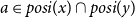 $a\in{posi}(x)\cap{posi}(y)$
.
$a\in{posi}(x)\cap{posi}(y)$
.
 $F(\mathbb T)$
is a monoid of chunks by Proposition 5.1.3, and since
$F(\mathbb T)$
is a monoid of chunks by Proposition 5.1.3, and since
 $x\bullet y\in\textsf{Chunk}_{\mathbb T}$
it follows that
$x\bullet y\in\textsf{Chunk}_{\mathbb T}$
it follows that
 $x\bullet y<\textsf{f}_{F(\mathbb T)}$
. It follows from Definition 4.3.1 that
$x\bullet y<\textsf{f}_{F(\mathbb T)}$
. It follows from Definition 4.3.1 that
 $y\in{rightB}(x)$
and
$y\in{rightB}(x)$
and
 $x\in{leftB}(y)$
.
$x\in{leftB}(y)$
.
The result now follows by Definition 4.3.9.
Proposition 5.5.4 Suppose
 $\mathbb T\in\textsf{IEUTxO}$
and
$\mathbb T\in\textsf{IEUTxO}$
and
 $x\in F(\mathbb T){\setminus}\{\textsf{f}\}$
(that is,
$x\in F(\mathbb T){\setminus}\{\textsf{f}\}$
(that is,
 $x\in\textsf{Chunk}_{\mathbb T}$
). Then:
$x\in\textsf{Chunk}_{\mathbb T}$
). Then:
 \begin{align*}\begin{array}{r@{\ }l}{left}(x)=&{utxi}(x)\setminus{blockedUtxi}(x)\\{right}(x)=&{utxo}(x)\setminus{blockedUtxo}(x)\\{up}(x)=&{stx}(x)\cup{blockedUtxi}(x)\cup{blockedUtxo}(x)\end{array}\end{align*}
Proof. We know by Lemma 5.3.1 that
 ${left}(x)\subseteq{utxi}(x)$
and
${left}(x)\subseteq{utxi}(x)$
and
 ${right}(x)\subseteq{utxo}(x)$
. Now suppose
${right}(x)\subseteq{utxo}(x)$
. Now suppose
 $a\in{utxi}(x)$
and
$a\in{utxi}(x)$
and
 $a\not\in{blockedUtxi}(x)$
; unpacking Definition 5.5.1 this means that there exists a
$a\not\in{blockedUtxi}(x)$
; unpacking Definition 5.5.1 this means that there exists a
 $y\in\textsf{Chunk}_{\mathbb T}$
such that
$y\in\textsf{Chunk}_{\mathbb T}$
such that
 $a\in{utxo}(y)$
and
$a\in{utxo}(y)$
and
 $y\bullet x\in\textsf{Chunk}_{\mathbb T}$
. By Lemma 5.5.3 it follows that (
$y\bullet x\in\textsf{Chunk}_{\mathbb T}$
. By Lemma 5.5.3 it follows that (
 $a\in{right}(y)$
and)
$a\in{right}(y)$
and)
 $a\in{left}(x)$
.
$a\in{left}(x)$
.
The case of
 ${right}(x)$
is similar, and the case of
${right}(x)$
is similar, and the case of
 ${up}(x)$
follows from the previous two cases and Lemma 5.3.1.
${up}(x)$
follows from the previous two cases and Lemma 5.3.1.
6. The Functor
$G:\textsf{ACS}\to\textsf{IEUTxO}$

6.1 A brief discussion: why represent?
In Subsection 4.4.2, we observed a hierarchy of models, from concrete EUTxO structures to IEUTxO models to abstract chunk systems.
The mapping from IEUxO to ACS is the functor
 $F:\textsf{IEUTxO}\to\textsf{ACS}$
from Section 5. We will now exhibit a functor
$F:\textsf{IEUTxO}\to\textsf{ACS}$
from Section 5. We will now exhibit a functor
 $G:\textsf{ACS}\to\textsf{IEUTxO}$
back down from the abstract to the concrete structures.
Footnote 35
$G:\textsf{ACS}\to\textsf{IEUTxO}$
back down from the abstract to the concrete structures.
Footnote 35
This is interesting for two reasons: one specific and one general. We consider each in turn.
G is interesting because:
-
1. It gives a sense in which the abstraction reasonably represents the concrete models. That is, there is nothing the abstract model could do that is so crazy that it cannot be engineered back down to a concrete structure. This may involve some ugly concrete fiddling, emulation and choices – as one might expect going from an abstract to a concrete object – but it can be done, and seeing how, can be helpful for understanding both worlds.
-
2. Sometimes, theorems are better proved in the concrete world than the abstract world. This can be particularly useful to prove negative properties, that something cannot happen in the abstract world, because it would correspond to something that would be impossible in the concrete world. A well-known example is that every Boolean Algebra can be represented as a power set, and thus, every finite Boolean Algebra has cardinality a power of two. Thus, to prove that some abstract structure does not admit any Boolean Algebra structure, it suffices if its carrier set is finite and has cardinality that is not a power of two. Footnote 36
Now to understand the relevance of G specifically for this paper, consider the following question: In what sense is Definition 4.5.1 a good abstraction of Definition 3.1.2?
Design decisions are embedded in the conditions of Definition 4.5.1, and some of these were not trivial and had more than one plausible outcome. Why did we choose as we did? How do these choices interact? In what sense were they appropriate?
To answer these questions, F is not necessarily the greatest help on its own. To illustrate why, consider that we can obtain a general ‘theory of blockchains’ merely by insisting that an ‘abstract chunk system’ is a set. We impose no further structure: et voilÀ: instant generality! Footnote 37 But this tells us little; for example F would just be the forgetful functor, mapping an IEUTxO model to its underlying set. We could map just to monoids, if we add the failure element, and again an F would exist, but this would be only slightly less uninformative.
So where is the sweet spot, and why? As we observed, merely exhibiting an F-style functor does not help: we need to get an algebraic measure of what it is about Figure 1 that gives it its essential nature.
We get a formally meaningful measure of an appropriate level of abstraction by locating one at which we can build a sensible functor G going back, and seeing how conditions in Definition 4.5.1 interact with its construction – and, we can observe how tweaking them can affect, or even break, these constructions. A discussion of such tweaks, and their effects, is in Remarks 6.4.4 and 7.1.5, and Proposition 7.3.6.
Remark 6.1.1
((Comment on design)) What counts as a ‘sensible’ G is a design decision in itself. We consider several options in this paper (listed here in increasing order of size of the category of denotations
 $\textsf{ACS}$
):
$\textsf{ACS}$
):
-
1. a categorical equivalence (Proposition 7.3.6); or
-
2. a categorical embedding (Theorem 7.3.4 and Remark 7.3.5); or
-
3. just an injection on objects (Remark 6.4.4).
All these possibilities are justifiable.Footnote 38 So to be clear: G and the choices we make in building it are not intended as direct value judgements; they are a way to measure and explore the structure of a large, abstract and interesting design space.
6.2 Action on objects
Recall from Definition 3.1.2 the notion of an IEUTxO model, and the accompanying discussion in Remark 3.1.8 about the status of the injection
 $\nu:\textsf{Validator}\hookrightarrow{pow}(\beta\times\textsf{Transaction}_!)$
.
$\nu:\textsf{Validator}\hookrightarrow{pow}(\beta\times\textsf{Transaction}_!)$
.
Continuing that Remark, in Definition 6.2.1 we must be explicit about
 $\nu$
:
$\nu$
:
Definition 6.2.1 Suppose
 $(\textsf X,\textsf{e},\textsf{f},\leq,\bullet)\in\textsf{ACS}$
. We define an IEUTxO model
$(\textsf X,\textsf{e},\textsf{f},\leq,\bullet)\in\textsf{ACS}$
. We define an IEUTxO model
 $G(\textsf X)$
 \begin{align*}G(\textsf X)=(\alpha,\beta,\textsf{Transaction},\textsf{Validator},\nu:\textsf{Validator}\hookrightarrow{pow}(\beta\times\textsf{Transaction}_!))\end{align*}
as follows:
-
1. We take
$\alpha=\beta={atomic}(\textsf X)$
(Definition 4.1.4). -
2. We take:
where
\begin{align*}\textsf{Validator}=\{\ast\}\end{align*}
$\{\ast\}$
is a unit type.
-
3. For each atomic
$x\in{atomic}(\textsf X),$
we admit a transaction such that:
\begin{align*}\textsf{tx}(x)\in\textsf{Transaction}\end{align*}
Thus,
\begin{align*}\begin{array}{r@{\ }l}{input}(\textsf{tx}(x)) =& \{(a,x) \mid a\in{left}(x)\}\\{output}(\textsf{tx}(x)) =&\{(b,x,\ast)\mid b\in{right}(x)\cup{up}(x)\} .\end{array}\end{align*}
for
\begin{align*}\textsf{Transaction} = \{\textsf{tx}(X) \mid x\in{atomic}(\textsf X)\}\end{align*}
$\textsf{tx}$
defined as above.
-
4. We define
$\nu:\textsf{Validator}\hookrightarrow{pow}(\beta\times\textsf{Transaction}_!)$
to map
$\ast\in\textsf{Validator}$
as follows (
$\text{@} i$
from Notation 3.1.3): Thus,
\begin{align*}\nu(\ast) =\{(x,{tx}\text{@} (p,y)) \mid (p,y)\in{input}({tx}),\ x\bullet y<\textsf{f}\} .\end{align*}
$\nu(\ast)$
is the function that inputs x and a pointed transaction
${tx}\text{@} (p,y)$
, extracts the data y from the input, and then checks that
$x\bullet y<\textsf{f}$
in
$\textsf X$
.Footnote 39


Remark 6.2.2 Continuing Remark 3.8.1, we see that the validator used by G in Definition 6.2.1 is UTxO style; it only examines the (pointed) input of the transaction to be validated. So in fact, G maps not just to IEUTxO models but to the IUTxO models noted in Subsection 3.8. We will use this observation in Theorem 7.3.4(3).
An easy sanity check:
Lemma 6.2.3 Suppose
 $\textsf X\in\textsf{ACS}$
and
$\textsf X\in\textsf{ACS}$
and
 $x,y\in\textsf X$
. Then
$x,y\in\textsf X$
. Then
 $\textsf{tx}(x)\bullet\textsf{tx}(y)$
is a chunk if and only if
$\textsf{tx}(x)\bullet\textsf{tx}(y)$
is a chunk if and only if
 $x\bullet y<\textsf{f}$
.
$x\bullet y<\textsf{f}$
.
Proof. By construction, unravelling Definition 6.2.1.
Remark 6.2.4 ((Comment on design)) In Definition 6.2.1(3) we set
-
•
${input}(\textsf{tx}(x)) = \{(a,x) \mid a\in{left}(x)\}$
and -
•
${output}(\textsf{tx}(x)) =\{(b,x,\ast)\mid b\in{right}(x)\cup{up}(x)\}$
.


So
 ${up}$
-atoms in x map to
${up}$
-atoms in x map to
 ${output}$
-atoms in
${output}$
-atoms in
 $\textsf{tx}(x)$
. Why? For two reasons:
$\textsf{tx}(x)$
. Why? For two reasons:
-
• The short reason is that it makes Lemma 6.3.2 work: all atoms in
${posi}(x)$
get recorded in an input or output (even the ones in
${up}(x)$
, which cannot participate in a non-failing interaction), along with a copy of x (to get injectivity). -
• The longer reason is as follows: An ACS element
$x\in\textsf X$
has no internal structure and thus no explicit structural notion of inputs or outputs. Our only interaction with x is by combining it with other elements and observing partiality (cf. Remark 4.3.5). But suppose our ACS
$\textsf X$
was obtained concretely from an IEUTxO model using F from Definition 5.1.1, so that x is ‘secretly’ a singleton chunk, presented as an atomic element in an ACS. Then
$p\in{up}(x)$
could occur for two reasons: -
• either p is the position of an input which no output will accept (perhaps it is labelled with some data that all validators disapprove of);
-
• or p is the position of an output that will not validate any available input (e.g. it has the empty validator). When we come to map x back to a transaction
$\textsf{tx}(x)$
, the simplest way to record p is to attach it to an IEUTxO output located at p, with a validator that always fails.


The other option would be to attach p to an input in
 $\textsf{tx}(x)$
, to tag the data carried by that input with some special ‘fail-me’ tag and remember to create only validators that recognise this tag and reject the input. But this is clearly a more complicated way of doing things, and the design adopted in Definition 6.2.1(3) seems the natural and simple approach.
$\textsf{tx}(x)$
, to tag the data carried by that input with some special ‘fail-me’ tag and remember to create only validators that recognise this tag and reject the input. But this is clearly a more complicated way of doing things, and the design adopted in Definition 6.2.1(3) seems the natural and simple approach.
Several things about Definition 6.2.1 need checked. We start with Lemma 6.2.5:
Lemma 6.2.5
-
1. If
$\textsf X\in\textsf{ACS}$
and
$x\in{atomic}(\textsf X)$
then
$\textsf{tx}(x)$
has the right type to be a transaction as per Figure 1. -
2. If
$\textsf X\in\textsf{ACS}$
and
$x\in{atomic}(\textsf X)$
then
$[\textsf{tx}(x)]$
is a chunk. -
3. As a corollary, atomic elements in
$F(\textsf X)$
are precisely the singleton chunks of
$\textsf{tx}(x)$
, where x ranges over atomic elements of
$\textsf X$
– or more concisely in symbols:
\begin{align*}{atomic}(F(\textsf X))=\{[\textsf{tx}(x)]\mid x\in{atomic}(\textsf X)\}.\end{align*}


Proof.
-
1. From Definitions 4.4.1(1) and 6.2.1(3) and Lemma 4.3.12,
$\textsf{tx}(x)$
has finitely many inputs and outputs; so as per Figure 1 it is indeed a pair of a finite set of inputs and a finite set of outputs. -
2. By Lemma 3.4.6, to show
$[\textsf{tx}]$
is a valid chunk it would suffice to show that
${input}(\textsf{tx}(x))\cap{output}(\textsf{tx}(x))=\varnothing$
. This follows from Lemma 4.3.12 and Corollary 4.4.5. -
3. By construction and Lemma 4.1.6, noting that in lists ordered by subset inclusion, atomic elements are singleton lists.


Remark 6.2.6 ((Comment on design)) We mention an alternative definition of G from Definition 6.2.1, just to illustrate that more than one encoding is possible:
-
1. We take
$\alpha=\beta=\textsf{Validator}={atomic}(\textsf X)$
(Definition 4.1.4). -
2. For each atomic
$x\in{atomic}(\textsf X),$
we admit a transaction
$\textsf{tx}(x)\in\textsf{Transaction}$
such that:
\begin{align*}\begin{array}{r@{\ }l}{input}(\textsf{tx}(x)) =& \{(a,x) \mid a\in{left}(x)\}\\{output}(\textsf{tx}(x)) =&\{(b,x,x)\mid b\in{right}(x)\cup{up}(x)\}\end{array}\end{align*}
-
3. We define
$\nu:\textsf{Validator}\hookrightarrow{pow}(\beta\times\textsf{Transaction}_!)$
to map
$x\in\textsf{Validator}$
as follows:
\begin{align*}\nu(x) =\{(x,\textsf{tx}(y)\text{@} i) \mid x\bullet y<\textsf{f},\ i\in{input}(\textsf{tx}(y))\} .\end{align*}


Remark 6.2.7 It remains to prove that
 $\nu$
is well-defined and (as required by Definition 3.1.2(5)) is injective, and that
$\nu$
is well-defined and (as required by Definition 3.1.2(5)) is injective, and that
 $G(\textsf X)$
is indeed an IEUTxO model. See Corollaries 6.3.3 and 6.3.4.
$G(\textsf X)$
is indeed an IEUTxO model. See Corollaries 6.3.3 and 6.3.4.
6.3
$\nu$
is injective

Lemma 6.3.1 Suppose
 $\textsf X\in\textsf{ACS}$
(Definition 4.5.2). Then
$\textsf X\in\textsf{ACS}$
(Definition 4.5.2). Then
 \begin{align*}x\in{atomic}(\textsf X)\quad\text{implies}\quad{posi}(x)\neq\varnothing.\end{align*}
Proof. Suppose x is atomic. By Definition 4.1.4(1)
 $x\not\in\{\textsf{e},\textsf{f}\}$
. We use Lemma 4.4.3.
$x\not\in\{\textsf{e},\textsf{f}\}$
. We use Lemma 4.4.3.
Lemma 6.3.2 Suppose
 $\textsf X\in\textsf{ACS}$
. Then:
$\textsf X\in\textsf{ACS}$
. Then:
-
1. The assignment
from Definition 6.2.1(3) is injective.
\begin{align*}x\in{atomic}(\textsf X) \longmapsto \textsf{tx}(x) \in \textsf{Transaction}_{G(\textsf X)}\end{align*}
-
2.
${posi}(x)={pos}(\textsf{tx}(x))$
.


Proof.
-
1. By Lemma 6.3.1 (since x is atomic)
${posi}(x)\neq\varnothing$
, so by Lemma 4.3.12 at least one of
${left}(x)$
or
${right}(x)$
or
${up}(x)$
must be nonempty. If
${left}(x)$
is nonempty then
$\textsf{tx}(x)$
has an input and we can read x off the data in that input. Otherwise,
$\textsf{tx}(x)$
has an output and we can read x off the data in that output. -
2. It follows from Definition 6.2.1(3) and Figure 4 that
${pos}(\textsf{tx}(x))={left}(x)\cup({right}(x)\cup{up}(x))$
. Also, by Lemma 4.3.12
${pos}(x)={left}(x)\cup{right}(x)\cup{up}(x)$
.


As promised in Remark 6.2.7, we prove:
Corollary 6.3.3 The map
 \begin{align*}\nu:\textsf{Validator}\hookrightarrow{pow}(\beta\times\textsf{Transaction}_!)\end{align*}
from Definition 6.2.1(1) is well-defined and injective.
Proof. By Lemma 6.3.2(1), we can deduce y from
 $\textsf{tx}(y)$
. The result follows.
$\textsf{tx}(y)$
. The result follows.
Corollary 6.3.4 If
 $\textsf X$
is an abstract chunk system (Definition 4.5.1) then
$\textsf X$
is an abstract chunk system (Definition 4.5.1) then
 $G(\textsf X)$
is an IEUTxO model (Definition 3.1.2).
$G(\textsf X)$
is an IEUTxO model (Definition 3.1.2).
Proof. We just need to check the conditions of Definition 3.1.2; the only nontrivial part is that
 $\nu$
is an injection, and that is Corollary 6.3.3.
$\nu$
is an injection, and that is Corollary 6.3.3.
6.4 Action on arrows
Definition 6.4.1 Suppose
 $g:\textsf X\to\textsf Y\in\textsf{ACS}$
and recall from Definition 3.7.1(2) that an arrow
$g:\textsf X\to\textsf Y\in\textsf{ACS}$
and recall from Definition 3.7.1(2) that an arrow
 \begin{align*}G(g)=G(\textsf X)\to G(\textsf Y) \in \textsf{IEUTxO}\end{align*}
should be a mapping from
 $\textsf{Transaction}_{G(\textsf X)}$
to
$\textsf{Transaction}_{G(\textsf X)}$
to
 $\textsf{Chunk}_{G(\textsf Y)}$
. Recall
$\textsf{Chunk}_{G(\textsf Y)}$
. Recall
 ${factor}$
from Definition 4.2.5(1b), which factorises non-failure elements into atomic constituents, and recall from Definition 4.5.2(2b) that g maps non-failure elements to non-failure elements.
${factor}$
from Definition 4.2.5(1b), which factorises non-failure elements into atomic constituents, and recall from Definition 4.5.2(2b) that g maps non-failure elements to non-failure elements.
Then define G(g) by
 \begin{multline*}G(g) : \textsf{tx}(x) \longmapsto \textsf{tx}(y_1)\bullet\ldots\bullet \textsf{tx}(y_n)\in\textsf{Chunk}_{G(\textsf Y)}\\\quad\text{where}\quad {factor}(g(x))=[y_1,\dots,y_n]\in[{atomic}(\textsf Y)].\end{multline*}
Lemma 6.4.2 G(g) from Definition 6.4.1 is well-defined.
Proof. We must check that
 $\textsf{tx}(y_1)\bullet\ldots\bullet \textsf{tx}(y_n)$
is a chunk; this follows by Lemma 3.7.2.
$\textsf{tx}(y_1)\bullet\ldots\bullet \textsf{tx}(y_n)$
is a chunk; this follows by Lemma 3.7.2.
Proposition 6.4.3 The map G, with the action on abstract chunk systems from Definition 6.2.1, and with the action on arrows from Definition 6.4.1, is a functor
 \begin{align*}G : \textsf{ACS}\to\textsf{IEUTxO} .\end{align*}
Proof. Given the results above, the only remaining thing to check is that if
 $g:\textsf X\to \textsf Y$
and
$g:\textsf X\to \textsf Y$
and
 $g':\textsf Y\to\textsf Z$
then
$g':\textsf Y\to\textsf Z$
then
 $G(g'\,g)=G(g')G(g)$
. This follows by a routine argument from the definitions, using Definition 4.2.5(1(b)ii).
$G(g'\,g)=G(g')G(g)$
. This follows by a routine argument from the definitions, using Definition 4.2.5(1(b)ii).
Remark 6.4.4 ((Comment on design)) The significance of condition 1b of Definition 4.2.5 is not that elements can be factored into atomic elements – this follows already from condition 1b – but that a factorisation can be selected, as a monoid homomorphism.
We use this condition in just one place: to define the action of G on arrows in Definition 6.4.1 and prove it functorial in Proposition 6.4.3.
It would be legitimate to remove condition 1b of Definition 4.2.5. This would exhibit our category
 $\textsf{ACS}$
as a subcategory of a larger category which would include more objects – ‘even more abstract’ abstract chunk systems – at a cost of no longer being able to functorially map this larger space back down to
$\textsf{ACS}$
as a subcategory of a larger category which would include more objects – ‘even more abstract’ abstract chunk systems – at a cost of no longer being able to functorially map this larger space back down to
 $\textsf{IEUTxO}$
.
$\textsf{IEUTxO}$
.
Intuitively, this larger space behaves more like a space of all possible denotations rather than a space of
 $\textsf{IEUTxO}$
-representable ones, which might be worthwhile if it admits other interesting examples; whether or not this will be the case cannot be predicted at time of writing.
$\textsf{IEUTxO}$
-representable ones, which might be worthwhile if it admits other interesting examples; whether or not this will be the case cannot be predicted at time of writing.
Note that the action on objects from Definition 6.2.1 would still be well-defined even without Definition 4.2.5(1b), so that we can still represent our ‘even more abstract’ abstract chunk systems concretely in IEUTxO models: this just would not correspond to a functor. Footnote 40
7. An Adjunction between
$F:\textsf{IEUTxO}\to\textsf{ACS}$
: and
$G:\textsf{ACS}\to\textsf{IEUTxO}$


7.1 The counit map
$\epsilon_{\textsf X}:FG(\textsf X)\to\textsf X$
exists and is a surjection
Remark 7.1.1 Suppose
 $\textsf X\in\textsf{ACS,}$
we wish to define an arrow
$\textsf X\in\textsf{ACS,}$
we wish to define an arrow
 $\epsilon_{\textsf X}:FG(\textsf X)\to\textsf X\in\textsf{ACS}$
. Unpacking Definitions 6.2.1 and 5.1.1, we see that an
$\epsilon_{\textsf X}:FG(\textsf X)\to\textsf X\in\textsf{ACS}$
. Unpacking Definitions 6.2.1 and 5.1.1, we see that an
 $x\in FG(\textsf X)$
has one of the following forms:
$x\in FG(\textsf X)$
has one of the following forms:
-
•
$x={fail}_{FG(\textsf X)}$
for
${fail}_{FG(\textsf X)}$
the failure element added by F to
$\textsf{Chunk}_{G(\textsf X)}$
in Definition 5.1.1. -
•
$x=[\textsf{tx}(x_1),\dots,\textsf{tx}(x_n)]$
for some unique
$[x_1,\dots,x_n]\in[{atomic}(\textsf X)]$
.


We also know from Lemma 6.3.2 that
 $\textsf{tx}:{atomic}(\textsf X)\to\textsf{Transaction}(G(\textsf X))$
is injective, and it follows that we can recover each
$\textsf{tx}:{atomic}(\textsf X)\to\textsf{Transaction}(G(\textsf X))$
is injective, and it follows that we can recover each
 $x_i$
from the unique corresponding
$x_i$
from the unique corresponding
 $[\textsf{tx}(x_i)]$
above.
$[\textsf{tx}(x_i)]$
above.
Definition 7.1.2 Let
 $\epsilon_{\textsf X}:FG(\textsf X)\to\textsf X$
be determined by:
$\epsilon_{\textsf X}:FG(\textsf X)\to\textsf X$
be determined by:
-
1.
$\epsilon_{\textsf X}([])=\textsf{e}_{\textsf X}$
(this would be a special case of the next clause, for
$n=0$
) -
2.
$\epsilon_{\textsf X}([\textsf{tx}(x_1),\dots,\textsf{tx}(x_n)]) = x_1\bullet\ldots\bullet x_n$
for
$n\geq 1$
and
$x_1,\dots,x_n\in{atomic}(\textsf X)$
-
3.
$\epsilon_{\textsf X}(\textsf{f}_{FG(\textsf X)}) = \textsf{f}_{\textsf X}$


Lemma 7.1.3 Definition 7.1.2 is well-defined and determines an arrow in
 $\textsf{ACS}$
.
$\textsf{ACS}$
.
Proof. Well-definedness follows as per Remark 7.1.1 from Lemma 6.3.2, since we can recover each
 $x_i$
from its
$x_i$
from its
 $[\textsf{tx}(x_i)]$
. It remains to check the arrow conditions from Definition 4.5.2(2):
$[\textsf{tx}(x_i)]$
. It remains to check the arrow conditions from Definition 4.5.2(2):
-
1. We check that
$\epsilon_{\textsf X}(\textsf{e}_{FG(\textsf X)})=\textsf{e}_{\textsf X}$
and
$\epsilon(\textsf{f}_{FG(\textsf X)})=\textsf{f}_{\textsf X}$
. A fact of Definition 7.1.2. -
2. We check that
$x\leq y<\textsf{f}_{FG(\textsf X)}$
implies
$\epsilon_{\textsf X}(x)\leq \epsilon_{\textsf X}(y)<\textsf{f}_{\textsf X}$
. By Proposition 5.1.3,
$FG(\textsf X)$
is perfectly atomic, and if
$x\leq y<\textsf{f}_{FG(\textsf X)}$
then x and y factorise uniquely into a composition of lists of singleton chunks, which by construction in Definition 6.2.1(3) have the form
$\textsf{tx}(x_i)$
and
$\textsf{tx}(y_j)$
, such that the factorisation of x is a sublist of the factorisation of y. The result follows by a routine calculation from Definition 7.1.2. -
3.
$\epsilon_{\textsf X}(x)\bullet \epsilon_{\textsf X}(y)= \epsilon_{\textsf X}(x\bullet y)$
A fact of Definition 7.1.2, again using the fact that by Proposition 5.1.3
$FG(\textsf X),$
is perfectly atomic.


Proposition 7.1.4 The counit map
 $\epsilon_{\textsf X}:FG(\textsf X)\to\textsf X\in\textsf{ACS}$
is a surjection on underlying sets.
$\epsilon_{\textsf X}:FG(\textsf X)\to\textsf X\in\textsf{ACS}$
is a surjection on underlying sets.
Proof. Suppose we are given
 $x\in\textsf X$
, we want to exhibit an element in
$x\in\textsf X$
, we want to exhibit an element in
 $FG(\textsf X)$
that maps to it under
$FG(\textsf X)$
that maps to it under
 $\epsilon_{\textsf X}$
.
$\epsilon_{\textsf X}$
.
If
 $x=\textsf{f}_{\textsf X}$
then by construction in Definition 5.1.1
$x=\textsf{f}_{\textsf X}$
then by construction in Definition 5.1.1
 ${fail}_{FG(\textsf X)} = \textsf{f}_{FG(\textsf X)}$
and also by construction
${fail}_{FG(\textsf X)} = \textsf{f}_{FG(\textsf X)}$
and also by construction
 $\epsilon_{\textsf X}({fail}_{FG(\textsf X)})=\textsf{f}_{\textsf X}$
so we are done.
$\epsilon_{\textsf X}({fail}_{FG(\textsf X)})=\textsf{f}_{\textsf X}$
so we are done.
Otherwise by Proposition 5.1.3 (or just by Definition 4.2.5), we can write
 \begin{align*}x=x_1\bullet\ldots\bullet x_n\end{align*}
for some atomic
 $x_1,\dots,x_n\in{atomic}(\textsf X)$
, and looking at Definition 7.1.2 we immediately have that
$x_1,\dots,x_n\in{atomic}(\textsf X)$
, and looking at Definition 7.1.2 we immediately have that
 \begin{align*}\epsilon_{\textsf X} ([\textsf{tx}(x_1),\dots,\textsf{tx}(x_n)]) = x_1\bullet\ldots\bullet x_n = x.\end{align*}
Remark 7.1.5
((Comment on design)) By Proposition 7.1.4,
 $\epsilon_{\textsf X}$
surjects
$\epsilon_{\textsf X}$
surjects
 $FG(\textsf X)$
onto
$FG(\textsf X)$
onto
 $\textsf X$
as sets, but is it not necessarily surjective on the
$\textsf X$
as sets, but is it not necessarily surjective on the
 $\leq$
structure, meaning that
$\leq$
structure, meaning that
 $\epsilon_{\textsf X}({ch})\leq_{\textsf X}\epsilon_{\textsf X}({ch}')$
does not imply
$\epsilon_{\textsf X}({ch})\leq_{\textsf X}\epsilon_{\textsf X}({ch}')$
does not imply
 ${ch}\leq_{FG(\textsf X)} {ch}'$
.
${ch}\leq_{FG(\textsf X)} {ch}'$
.
We can have this if we add condition 2b of Definition 4.2.5, that: if
 $x\leq y<\textsf{f}$
then
$x\leq y<\textsf{f}$
then
 ${factor}(x)\leq{factor}(y)$
(the right-hand
${factor}(x)\leq{factor}(y)$
(the right-hand
 $\leq$
denotes sublist inclusion; the left-hand
$\leq$
denotes sublist inclusion; the left-hand
 $\leq$
is the partial order on
$\leq$
is the partial order on
 $\textsf X$
). More on this in Proposition 7.3.6. Further tweaks to the design of abstract chunk systems are also mentioned in Remark 6.4.4.
$\textsf X$
). More on this in Proposition 7.3.6. Further tweaks to the design of abstract chunk systems are also mentioned in Remark 6.4.4.
7.2 The unit map
$\eta_{\mathbb T}:\mathbb T\to \mathrm{GF}(\mathbb T)$
exists and is an isomorphism

Remark 7.2.1 Suppose
 $\mathbb T=(\alpha,\beta,\textsf{Transaction},\textsf{Validator})\in\textsf{IEUTxO}$
. We wish to define an arrow
$\mathbb T=(\alpha,\beta,\textsf{Transaction},\textsf{Validator})\in\textsf{IEUTxO}$
. We wish to define an arrow
 \begin{align*}\eta_{\mathbb T}:\mathbb T\to \mathrm{GF}(\mathbb T) .\end{align*}
We can make some observations:
-
• By construction in Definition 5.1.1,
$F(\mathbb T)$
is isomorphic as a partial ordering to
$\mathbb T$
, with the addition of the
${fail}$
top element. As noted in Proposition 5.1.3, it follows that the atomic elements of
$F(\mathbb T)$
correspond precisely with the singleton chunks in
$\textsf{Chunk}_{\mathbb T}$
and thus with transactions in
$\textsf{Transaction}_{\mathbb T}$
. The chunks in
$F(\mathbb T)$
are then determined by combining the singleton chunks, subject to the well-formedness conditions of Definition 3.4.1 and the locality properties noted in Lemma 3.5.1. -
• By construction in Definition 6.2.1, the atomic elements of
$\mathrm{GF}(\mathbb T)$
are isomorphic to
${atomic}(F(\mathbb T))$
, and by Lemma 6.2.5(3) also to
$\textsf{Transaction}_{\mathbb T}$
.


Definition 7.2.2 Let
 $\eta_{\mathbb T}:\mathbb T\to \mathrm{GF}(\mathbb T)$
be determined by mapping
$\eta_{\mathbb T}:\mathbb T\to \mathrm{GF}(\mathbb T)$
be determined by mapping
 ${tx}\in\textsf{Transaction}_{\mathbb T}$
to
${tx}\in\textsf{Transaction}_{\mathbb T}$
to
 $[\textsf{tx}({tx})]\in \textsf{Chunk}_{\mathrm{GF}(\mathbb T)}$
. Thus using Lemma 3.7.2 we have:
$[\textsf{tx}({tx})]\in \textsf{Chunk}_{\mathrm{GF}(\mathbb T)}$
. Thus using Lemma 3.7.2 we have:
 \begin{align*}\eta_{\mathbb T}([{tx}_1,\dots,{tx}_n]) = [\textsf{tx}({tx}_1),\dots,\textsf{tx}({tx}_n)] .\end{align*}
Lemma 7.2.3 If
-
•
$x=[{tx}_1,\dots,{tx}_n]\in\textsf{Chunk}_{\mathbb T}$
, then -
•
$\eta_{\mathbb T}(x)=[\textsf{tx}({tx}_1),\dots,\textsf{tx}({tx}_n)]\in\textsf{Chunk}_{\mathrm{GF}(\mathbb T)}$
.


As a corollary, Definition 7.2.2 does indeed map chunks to chunks.
Proof. By a routine check on Definition 6.2.1(3), using Proposition 5.5.4.
Lemma 7.2.4 Recall the notions of
 ${utxi}$
,
${utxi}$
,
 ${utxo}$
and
${utxo}$
and
 ${stx}$
from Definition 3.4.8 and the notion of
${stx}$
from Definition 3.4.8 and the notion of
 ${blockedUtxi}$
from Definition 5.5.1. Recall
${blockedUtxi}$
from Definition 5.5.1. Recall
 $\eta$
from Definition 7.2.2 and suppose
$\eta$
from Definition 7.2.2 and suppose
 $x\in\textsf X\in\textsf{ACS}$
. Then:
$x\in\textsf X\in\textsf{ACS}$
. Then:
-
1.
${utxi}(\eta_{\mathbb T}(x))={utxi}(x)\setminus{blockedUtxi}(x)$
-
2.
${utxo}(\eta_{\mathbb T}(x))={utxo}(x)\cup{blockedUtxi}(x)$
-
3.
${stx}(\eta_{\mathbb T}(x))={stx}(x)$


Proof. By routine calculations using Proposition 5.5.4.
Proposition 7.2.5 The unit map
 $\eta_{\mathbb T}:\textsf{Chunk}_{\mathbb T}\to \textsf{Chunk}_{\mathrm{GF}(\mathbb T)}\in\textsf{IEUTxO}$
is a bijection on underlying sets.
$\eta_{\mathbb T}:\textsf{Chunk}_{\mathbb T}\to \textsf{Chunk}_{\mathrm{GF}(\mathbb T)}\in\textsf{IEUTxO}$
is a bijection on underlying sets.
Proof. Using Lemma 6.3.2 and the fact that from Definitions 5.1.1 and 6.2.1, any element of
 $\mathrm{GF}(\mathbb T)$
has the form
$\mathrm{GF}(\mathbb T)$
has the form
 $[\textsf{tx}({tx}_1),\dots,\textsf{tx}({tx}_n)]$
for some transactions
$[\textsf{tx}({tx}_1),\dots,\textsf{tx}({tx}_n)]$
for some transactions
 ${tx}_1,\dots,{tx}_n\in\textsf{Transaction}_{\mathbb T}$
.
${tx}_1,\dots,{tx}_n\in\textsf{Transaction}_{\mathbb T}$
.
7.3 F is left adjoint to GG
Remark 7.3.1 Naturality of
 $\epsilon$
and
$\epsilon$
and
 $\eta$
is Propositions 7.3.2 and 7.3.3. The proofs are by diagram chasing. We do need to be a little careful because of the choice made in the
$\eta$
is Propositions 7.3.2 and 7.3.3. The proofs are by diagram chasing. We do need to be a little careful because of the choice made in the
 ${factor}$
function (Definition 4.2.5(1b)), which propagates to the action of G on arrows (Definition 4.1). In the event, the diagram chasing is all standard and it works fine.
Footnote 41
${factor}$
function (Definition 4.2.5(1b)), which propagates to the action of G on arrows (Definition 4.1). In the event, the diagram chasing is all standard and it works fine.
Footnote 41
Proposition 7.3.2 The counit map
 $\epsilon$
is a natural transformation from FG to
$\epsilon$
is a natural transformation from FG to
 $1_{\textsf{ACS}}$
.
$1_{\textsf{ACS}}$
.
Proof. Consider some arrow
 $g:\textsf X\to\textsf Y\in\textsf{ACS}$
. We must check a commuting square in
$g:\textsf X\to\textsf Y\in\textsf{ACS}$
. We must check a commuting square in
 $\textsf{ACS}$
that
$\textsf{ACS}$
that
 \begin{align*}\epsilon_{\textsf Y}\,FG(g) = g\,\epsilon_{FG(\textsf X)}.\end{align*}
Using Proposition 4.5.5(2) it suffices to check for each
 $x'\in{atomic}(FG(\textsf X))$
that
$x'\in{atomic}(FG(\textsf X))$
that
 \begin{align*}\epsilon_{\textsf Y}(FG(g)\,(x')) = g(\epsilon_{FG(\textsf X)}\,x').\end{align*}
From Lemma 6.2.5(3),
 $x'=[\textsf{tx}(x)]$
for
$x'=[\textsf{tx}(x)]$
for
 $x\in{atomic}(\textsf X)$
.
$x\in{atomic}(\textsf X)$
.
Write
 $g(x)=y_1\bullet\ldots\bullet y_n$
where
$g(x)=y_1\bullet\ldots\bullet y_n$
where
 ${factor}(g(x))=[y_1,\dots,y_n]\in[{atomic}(\textsf Y)]$
(Definition 4.2.5(1b)), so that
${factor}(g(x))=[y_1,\dots,y_n]\in[{atomic}(\textsf Y)]$
(Definition 4.2.5(1b)), so that
 \begin{align*}(FG(g))([\textsf{tx}(x)]) = [\textsf{tx}(y_1),\dots,\textsf{tx}(y_n)]\in FG(\textsf Y) .\end{align*}
Then
 \begin{align*}\epsilon_{\textsf Y}(FG(g)([\textsf{tx}(x)]))=\epsilon_{\textsf Y}([\textsf{tx}(y_1),\dots,\textsf{tx}(y_n)]) = y_1\bullet\ldots\bullet y_n = y\end{align*}
and
 \begin{align*}g(\epsilon_{\textsf X}([\textsf{tx}(x)])) =g(x) = y\end{align*}
as required.
Consider
 $f:\mathbb S\to\mathbb T$
and
$f:\mathbb S\to\mathbb T$
and
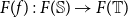 $F(f):F(\mathbb S)\to F(\mathbb T)$
and some
$F(f):F(\mathbb S)\to F(\mathbb T)$
and some
 $[{tx}]\in\textsf{Chunk}_{\mathbb S}$
and
$[{tx}]\in\textsf{Chunk}_{\mathbb S}$
and
 $f({tx})=[{tx}_1,\dots,{tx}_n]\in\textsf{Chunk}_{\mathbb T}$
. Then
$f({tx})=[{tx}_1,\dots,{tx}_n]\in\textsf{Chunk}_{\mathbb T}$
. Then
 $\eta_{\mathbb S}([{tx}_1,\dots,{tx}_n]) = [\textsf{tx}({tx}_1),\dots,\textsf{tx}({tx}_n)]$
and
$\eta_{\mathbb S}([{tx}_1,\dots,{tx}_n]) = [\textsf{tx}({tx}_1),\dots,\textsf{tx}({tx}_n)]$
and
 \begin{align*}F(f)([{tx}])\,([{tx}_1,\dots,{tx}_n])\end{align*}
Proposition 7.3.3 The unit map
 $\eta$
is a natural transformation from
$\eta$
is a natural transformation from
 $1_{\textsf{IEUTxO}}$
to GF.
$1_{\textsf{IEUTxO}}$
to GF.
Proof. Consider some arrow
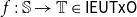 $f:\mathbb S\to\mathbb T\in\textsf{IEUTxO}$
. We must check a commuting square in
$f:\mathbb S\to\mathbb T\in\textsf{IEUTxO}$
. We must check a commuting square in
 $\textsf{IEUTxO}$
that
$\textsf{IEUTxO}$
that
 \begin{align*}\eta_{\mathbb T}\,f = \mathrm{GF}(f)\,\eta_{\mathbb S}.\end{align*}
Using Lemma 3.7.2 it suffices to check for each
 ${tx}\in\textsf{Transaction}_{\mathbb S}$
that
${tx}\in\textsf{Transaction}_{\mathbb S}$
that
 \begin{align*}\eta_{\mathbb T}(f([{tx}])) = \mathrm{GF}(f)(\eta_{\mathbb S}([{tx}])) .\end{align*}
Suppose
 $f({tx})=[{tx}_1,\dots,{tx}_n]\in\textsf{Chunk}_{\mathbb T}$
. Then
$f({tx})=[{tx}_1,\dots,{tx}_n]\in\textsf{Chunk}_{\mathbb T}$
. Then
 \begin{align*}\eta_{\mathbb T}(f([{tx}])) = \eta_{\mathbb T}([{tx}_1,\dots,{tx}_n]) = [\textsf{tx}({tx}_1),\dots,\textsf{tx}({tx}_n)]\end{align*}
and
 \begin{align*}\mathrm{GF}(f)(\eta_{\mathbb S}([{tx}]))=\mathrm{GF}(f)([\textsf{tx}({tx})])=[\textsf{tx}({tx}_1),\dots,\textsf{tx}({tx}_n)]\end{align*}
as required.
Theorem 7.3.4
-
1. The functors
from Definitions 5.1.1 and 5.4.1 (for F) and from Definitions 6.2.1 and 6.4.1 (for G) form an adjoint pair. In symbols:
\begin{align*}F:\textsf{IEUTxO}\to\textsf{ACS}\quad\text{and}\quad G:\textsf{ACS}\to\textsf{IEUTxO}\end{align*}
\begin{align*}F\dashv G : \textsf{IEUTxO}\to\textsf{ACS}\end{align*}
-
2. F is full and faithful (a bijection on homsets), and G is full (a surjection on homsets). Thus, F is a full embedding of
$\textsf{IEUTxO}$
into
$\textsf{ACS}$
.
Footnote 42
-
3. The image
$G(\textsf X)$
of
$\textsf X\in\textsf{ACS}$
is in fact a pure IUTxO model – meaning that its validators examine only the input-point of the transaction passed to them, not the entire transaction – and
$\textsf G$
maps more specifically to the full subcategory
$\textsf{IUTxO}$
of
$\textsf{IEUTxO}$
(Subsection 3.8). Thus, have the following short chain of maps (3)where on the left
\begin{equation}\textsf{IUTxO}\ \stackrel{{e}\ \dashv\ \mathrm{GF}}\longrightarrow\\textsf{IEUTxO}\ \stackrel{F\ \dashv\ G}\longrightarrow\\textsf{ACS}\end{equation}
${e}$
denotes the trivial inclusion/embedding map (Remark 3.8.1) with right adjoint GF.Footnote 43
-
4. The image
$\mathrm{GF}(\mathbb T)$
of
$\mathbb T\in\textsf{IEUTxO}$
is a pure IUTxO model and as a corollary, every IEUTxO model
$\mathbb T$
is isomorphic via
$\eta_{\mathbb T}:\mathbb T\to\mathrm{GF}(\mathbb T)$
to an IUTxO model
$\mathrm{GF}(\mathbb T)$
,


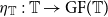

Proof.
-
1. The natural transformations are
$\epsilon:FG\to 1$
and
$\eta:1\to\mathrm{GF}$
from Definitions 7.1.2 and 7.2.2. They are natural by Propositions 7.3.2 and 7.3.3. -
2. By Proposition 7.2.5, the unit
$\eta$
is a bijection and it follows that f is full and faithful. By Proposition 7.1.4, the counit
$\epsilon$
is a surjection and it follows that G is full (this also follows from the fact that
$\eta$
is a bijection and so an injection). -
3. This is a structural fact of Definition 6.2.1, as observed in Remark 6.2.2.
-
4. From Proposition 7.2.5 and part 3 of this result.


Remark 7.3.5 We can present the diagram in (3) in Theorem 7.3.4(3) (recall that 1 and
 $\textsf{IUTxO}$
are from Subsection 3.8) quite nicely as a loop of embeddings:
$\textsf{IUTxO}$
are from Subsection 3.8) quite nicely as a loop of embeddings:
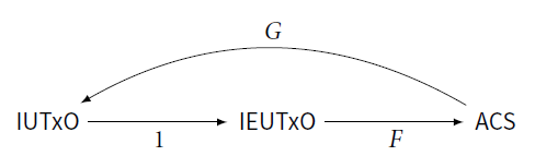
Intuitively,
 $\textsf{ACS}$
denotations seem to be the largest denotational class which conveniently maps back down into
$\textsf{ACS}$
denotations seem to be the largest denotational class which conveniently maps back down into
 $\textsf{IEUTxO}$
models as above (this is an intuitive observation, not a theorem). But if we wish to optimise differently and make our denotation more specific, then we can be rewarded with a tighter result:
$\textsf{IEUTxO}$
models as above (this is an intuitive observation, not a theorem). But if we wish to optimise differently and make our denotation more specific, then we can be rewarded with a tighter result:
Proposition 7.3.6 If we strengthen Definition 4.5.1 so that an abstract chunk system is a perfectly atomic oriented monoid of chunks (Definition 4.2.5(2)) instead of just being an atomic one, then
-
•
$\epsilon_{\textsf X}$
in Proposition 7.1.4 becomes a bijection, and -
• the embedding
$F\dashv G$
in Theorem 7.3.4 becomes an equivalence of categories, and -
• the loop illustrated in Remark 7.3.5 becomes a loop of equivalences. Thus, the full subcategory in
$\textsf{ACS}$
of perfectly atomic abstract chunk systems, and all arrows between them, is the ‘properly IEUTxO-like’ abstract chunk systems.
Footnote 44


Proof. The bijection is just a structural fact: if by Definition 4.2.5(2a) an element
 $x\in\textsf X\in\textsf{ACS}$
factorises uniquely into a list of atomic elements
$x\in\textsf X\in\textsf{ACS}$
factorises uniquely into a list of atomic elements
 $x_1\bullet \dots \bullet x_n$
, then x can be identified with that list and G just maps it to a list of transactions
$x_1\bullet \dots \bullet x_n$
, then x can be identified with that list and G just maps it to a list of transactions
 $[\textsf{tx}(x_1),\dots,\textsf{tx}(x_n)]$
– which, by design in Definition 6.2.1, has the same composition behaviour in
$[\textsf{tx}(x_1),\dots,\textsf{tx}(x_n)]$
– which, by design in Definition 6.2.1, has the same composition behaviour in
 $G(\textsf X)$
as x does in
$G(\textsf X)$
as x does in
 $\textsf X$
.
$\textsf X$
.
Then, Definition 4.2.5(2b) is exactly what is required for
 $FG(\textsf X)$
to ‘remember’ all the
$FG(\textsf X)$
to ‘remember’ all the
 $\leq$
-structure of
$\leq$
-structure of
 $\textsf X$
.
$\textsf X$
.
8. Conclusions
We have presented the EUTxO blockchain model in a novel and compact form and derived from it an algebra-style theory of blockchains as partially ordered partial monoids with channel name communication. This builds on previous work (BrÜnjes and Gabbay Reference BrÜnjes and Gabbay2020).
We hope this paper will make two contributions:
-
1. its specific definitions and theorems and also
-
2. an idea that blockchain structures can be subjected to this kind of analysis.
Or to put it another way: we illustrate that an algebraic theory of blockchains is possible, and what it might look like.
The reader can apply these ideas to their favourite blockchain architecture, and if this were widespread practice then this might help make the field accessible to an even broader audience, ease technical comparisons between systems, add clarity to a fast-changing field – and as we have argued, it might suggest structures and tests for practical programs, as is already reflected in a recent work (BrÜnjes and Gabbay Reference BrÜnjes and Gabbay2020; Gabbay Reference Gabbay2020b).
We now reflect on the design decisions made along the way and suggest possibilities for future work.
8.1 Observational equivalence
We touched on notions of observational equivalence in Subsections 3.5.2 and 4.3.3.
The theory of EUTxO observational equivalence is a little weaker than we might like, in the sense that not as many things get identified as one might first anticipate.
This is because a validator gets access to the whole transaction from which an input emanates – see the line for
 $\textsf{Validator}$
in Figure 1. (This is specific to EUTxO; UTxO is more local, see Remark 3.8.1.)
$\textsf{Validator}$
in Figure 1. (This is specific to EUTxO; UTxO is more local, see Remark 3.8.1.)
This makes it hard to factor out internal structure. For instance, even if all but one of the inputs and outputs of a transaction have been spent, so that it has just one dangling input – then that entire transaction is still observable at the final dangling input. Recall Proposition 3.5.12 and consider
 ${tx},{tx}'\in\textsf{Transaction}$
such that
${tx},{tx}'\in\textsf{Transaction}$
such that
 ${pos}({tx})\cap{pos}({tx}')=\varnothing$
, so that
${pos}({tx})\cap{pos}({tx}')=\varnothing$
, so that
 ${tx}$
and
${tx}$
and
 ${tx}'$
are commuting. We might reasonably wish to identify
${tx}'$
are commuting. We might reasonably wish to identify
 ${tx}\bullet{tx}'$
and
${tx}\bullet{tx}'$
and
 ${tx}'\bullet{tx}$
with a composite transaction which we might write
${tx}'\bullet{tx}$
with a composite transaction which we might write
 ${tx}\cup{tx}'$
, but we cannot do this because a validator could see the difference.
${tx}\cup{tx}'$
, but we cannot do this because a validator could see the difference.
Thus, currently the EUTxO framework can observe the difference between
-
• one large transaction and
-
• a composite chain (i.e. a chunk; see Definition 3.4.1) of smaller ones
– even if they are ‘morally’ the same. This is not good for developing compositional theories of observational equivalence.
We propose it might be helpful if the EUTxO model allowed us to limit access to the channels in a transaction, such that an input can limit validators to access only certain inputs and outputs in a transaction, for example by nominating positions that are ‘examinable’ along that input. Footnote 45 The pure UTxO model (Remark 3.8.1) would correspond to the special case when an input nominates only itself for validators to access.
Then, we would in suitable circumstances be able to switch between a single large transaction and a composite chunk with the same inputs and outputs.
Another observable of a transaction is the names of its spent transaction channels, and this brings us to garbage collection:
8.2 Garbage collection
Our model has no garbage collection of spent positions – where by spent positions we mean the
 ${stx}$
-atoms from Definition 3.4.8; see also the
${stx}$
-atoms from Definition 3.4.8; see also the
 ${up}$
-atoms from Definition 4.3.9 (a connection is precisely stated in Proposition 5.5.4).
${up}$
-atoms from Definition 4.3.9 (a connection is precisely stated in Proposition 5.5.4).
There is nothing wrong with this; the EUTxO presentation in Chakravarty et al. (Reference Chakravarty, Chapman, MacKenzie, Melkonian, Peyton Jones and Wadler2020) does not garbage-collect either (i.e. positions on the blockchain can be occupied at most once and can never be un-occupied).
However, since we name our positions, it might be nice to consider garbage-collecting (i.e. locally binding) the names of spent positions, by removing or
 $\alpha$
-converting them in some way. We do this in the implementation in Gabbay (Reference Gabbay2020b).
$\alpha$
-converting them in some way. We do this in the implementation in Gabbay (Reference Gabbay2020b).
However, the maths indicates that this does come at a certain price. For instance, consider a very simple model of finite lists of atoms in which the first atom is an ‘input’ and the last atom is an ‘output’, and we garbage-collect by removing matching atoms, like so:
 \begin{align*}[a,b]\bullet [b,c] = [a,c]\qquad[a,c]\bullet [c,b] = [a,b] .\end{align*}
Thus,
 \begin{align*}([a,b]\bullet [b,c])\bullet [c,b] = [a,b] .\end{align*}
Now if we bracket the other way, then
 $[b,c]\bullet [c,b]$
is ill-defined, and therefore, so is
$[b,c]\bullet [c,b]$
is ill-defined, and therefore, so is
 $[a,b]\bullet([b,c]\bullet [c,b])$
. We cannot have [b,b] because this would violate the condition that an input must point to an earlier (not a later) output (Definition 3.4.1(3); we consider relaxing this condition in item 2 of Subsection 8.6).
$[a,b]\bullet([b,c]\bullet [c,b])$
. We cannot have [b,b] because this would violate the condition that an input must point to an earlier (not a later) output (Definition 3.4.1(3); we consider relaxing this condition in item 2 of Subsection 8.6).
The partiality is no issue – chunks are already a partial monoid (Theorem 3.5.4). But, our monoid of garbage-collecting chunks would not be associative. It would still be nearly associative, meaning that
 $x\bullet (y\bullet z)=(x\bullet y)\bullet z$
where both sides are defined. However this is a weaker property that would be messier to work with, and for now we do not need it to make our case.
$x\bullet (y\bullet z)=(x\bullet y)\bullet z$
where both sides are defined. However this is a weaker property that would be messier to work with, and for now we do not need it to make our case.
This could also be read as a mathematical hint that our uniqueness conditions are a little too strict and that
 $[b,c]\bullet[c,b]$
should be permitted, where the leftmost b does not point to the later b but instead points backwards in time to some earlier b, and the rightmost b points forwards towards some later b – in the style of an interleaved scope (Gabbay et al. Reference Gabbay, Ghica, Petrisan and Kreutzer2015), for example. In the presence of garbage collection, this would make perfect sense, since we would expect both bs to eventually get bound, that is ‘spent’.
$[b,c]\bullet[c,b]$
should be permitted, where the leftmost b does not point to the later b but instead points backwards in time to some earlier b, and the rightmost b points forwards towards some later b – in the style of an interleaved scope (Gabbay et al. Reference Gabbay, Ghica, Petrisan and Kreutzer2015), for example. In the presence of garbage collection, this would make perfect sense, since we would expect both bs to eventually get bound, that is ‘spent’.
In this paper, we do not garbage-collect. We leave deciding whether we should, and if so how, for future work.
8.3 Tests
A few more words on the equations in Figure 1 (IEUTxO type equations) vs. those in Definition 5.2 (its algebraic counterpart of abstract chunk systems):
We want the equations in Figure 1 to be short and sweet, so that the system looks simple and solutions are easy to build and manipulate.
The design parameters in Definition 4.5.2 are somewhat different: we do not mind if there are plenty of algebraic properties, because this means that we have captured as many interesting properties as possible. The adjunction in Theorem 7.3.4 gives a formal sense in which the two correspond.
(This leaves it for future work to see how these conditions could be relaxed, as discussed e.g. in Remarks 6.4.4 and 7.1.5 and Proposition 7.3.6.)
This has mathematical interest, but not only that.
As noted in Subsection 4.4.2, modern programming languages support efficient programming on abstract denotations, thus delaying instantiating to specific instances until truly necessary. Also, they allow us to express and test against properties – and equality properties in particular can be helpful for optimising transformations.
So an algebraic theory can be relevant to producing concrete working code, because:
-
1. it can help structure code, and
-
2. an axiom can be read both as a testable property and as a program transformation; so that
-
3. the more axioms we have, the more transformations and tests are available, and the more scope we have to transform, structure, and test our programs.
8.4 Connections with nominal techniques
This paper borrows ideas from nominal techniques (Gabbay and Pitts Reference Gabbay and Pitts2001), and in particular, it follows the ideas on Equivariant ZFA from Gabbay (Reference Gabbay2020a) in handling the atoms which we use to name positions. We use atoms to name positions in IEUTxO models and in abstract chunk systems (ACS).
Partly, this is just using nominal-style names and permutations as a standard vocabulary. We can think of this application of nominal ideas as reaching for a familiar API, typeclass, or algebra, and there is nothing wrong with that.
The reader can find this implemented in Gabbay (Reference Gabbay2020b), where the IEUTxO equations in Figure 1 are combined with this author’s nominal data types package to create first a Haskell typeclass, and then a working implementation of chunks and blockchains, following the IEUTxO model of this paper.
But in parts of this paper, something deeper is also taking place. For example:
-
1. The notion of abstract chunk system – which makes up the more abstract half of this paper – depends on that of an oriented monoids of chunks from Definition 4.4.1, which depends on the notion of
${posi}$
from Definition 4.3.6, whose definition depends on the permutation action.
${posi}$
is a nameful definition, in the nominal sense, and it is not clear how would express it, and thus the notion of ACS, were it not for our nominal use of names. -
2. In Gabbay (Reference Gabbay2020b), we go somewhat further than in this paper in developing IEUTxO models, in that we permit
$\alpha$
-conversion to garbage-collect spent positions as discussed in Subsection 8.2. This too is a fully nominal definition, which uses the nominal model of binding in specific ways.


Remark 8.4.1
((No support assumed)) Experts on nominal techniques should note that no finite support conditions are imposed; for example, there is nothing to insist that a validator
 $\nu(v)\subseteq\beta\times\textsf{Transaction}_!$
should be a finitely-supported subset. This paper is in ZFA, not Fraenkel-Mostowski set theory.
$\nu(v)\subseteq\beta\times\textsf{Transaction}_!$
should be a finitely-supported subset. This paper is in ZFA, not Fraenkel-Mostowski set theory.
We could construct a finitely supported account of the theory in this paper in FM, just by imposing finite support conditions appropriately – but it would cost us complexity, and since we do not seem to need this, we do not do it. We hope we have struck a good balance in the mathematics between being rigorous in our treatment of names, and not drowning the reader in detail.
Note that finiteness conditions on sets of names are still important: notably in Definition 4.4.1(4.1), and name management is key to some nontrivial results, notably Corollary 4.4.5. So there is a ‘finite support’ flavour to the maths, just not as a direct translation of the Fraenkel-Mostowski notion of finite support.
Remark 8.4.2 ((Disjointness conditions)) Continuing the previous remark, ‘freshness-flavoured’ set disjointness conditions like
-
•
${input}({tx})\cap{output}({tx})=\varnothing$
in Lemma 3.4.6, and -
•
${pos}({ch})\cap{pos}({ch}')=\varnothing$
in Lemma 3.5.6, and -
•
${posi}(x)\cap{posi}(y)=\varnothing$
in Definition 4.4.1 and elsewhere, are quite important in this paper.


We could have imported a nominal notation and written these
 $\#$
, as in
$\#$
, as in
 ${ch}\#{ch}'$
or
${ch}\#{ch}'$
or
 $x\#y$
. This would not be wrong, but it might mislead because, as discussed above, we do not assume nominal notions of support and freshness. Thus,
$x\#y$
. This would not be wrong, but it might mislead because, as discussed above, we do not assume nominal notions of support and freshness. Thus,
 ${pos}({ch})$
and
${pos}({ch})$
and
 ${posi}(x)$
are not necessarily equal to the support of
${posi}(x)$
are not necessarily equal to the support of
 ${ch}$
and x, respectively, and if for example x and y were in an abstract chunk system that happened also to be finitely-supported (a plausible scenario), it would not be guaranteed that
${ch}$
and x, respectively, and if for example x and y were in an abstract chunk system that happened also to be finitely-supported (a plausible scenario), it would not be guaranteed that
 $x\#y$
would coincide with
$x\#y$
would coincide with
 ${posi}(x)\cap{posi}(y)=\varnothing$
.Footnote 46
${posi}(x)\cap{posi}(y)=\varnothing$
.Footnote 46
We could insist that
 ${supp}(x)$
must exist and coincide with
${supp}(x)$
must exist and coincide with
 ${posi}(x)$
, of course – but that would be an additional restriction.
${posi}(x)$
, of course – but that would be an additional restriction.
8.5 Concrete formalisation
Can we implement all or parts of this paper in a theorem-prover, and use that to verify properties of a blockchain system?
This paper has a lot of moving parts, and it is not all or nothing: a user can import whichever components (IEUTxO or ACS) they wish – though we also hope that the overall mathematical vision could provide useful guidance.
How the ideas in this paper might be brought to bear in the setting of a formal verification cannot have a clear-cut answer, because it depends on interactions between the maths, what we want to verify, the resources available, Footnote 47 and what facilities are offered by a particular theorem-proving environment.
A reasonable (but naive) implementation of the EUTxO inductive definition in Chakravarty et al. (Reference Chakravarty, Chapman, MacKenzie, Melkonian, Peyton Jones and Wadler2020) would suggest modelling positions by numbers which are essentially de Bruijn indices. The maths in this paper suggests against this:
-
• We want to talk about chunks. Indices only make sense in a blockchain which has an initial genesis block from which we start to index.
-
• We want to rearrange transactions and chunks, for example to talk about how they commute, as in (for example) Definition 4.3.16. With indices, a transaction in a different place is a different transaction, and potentially subject to different validation if a validator were to directly inspect its indices.
-
• Because we use names, we never have to worry about reindexing functions, as can be an issue with the de Bruijn indexed approach.
This is borne out by the practice: the developers of the EUTxO implementation underlying Chakravarty et al. (Reference Chakravarty, Chapman, MacKenzie, Melkonian, Peyton Jones and Wadler2020) have explored theorem-provers and they do not reference transactions by position (even though the mathematical description in the literature makes it look like they do, at least to the uninformed reader).
What they actually do is maintain an explicit naming context. This is ongoing research, but the interested reader can find a brief description in Melkonian et al. (Reference Melkonian, Swierstra and Chakravarty2019).
The difficulty with this hands-on context-based approach is that we end up having to curate our context of names, using explicit context-weakening and context-combining operations. These get limited, extremely tedious to formulate and prove, and clutter the proofs of properties. Footnote 48
It is standard and known that maintaining contexts of ‘known names’ can get painful. Indeed, this is one of the issues that nominal techniques were developed to alleviate.
In the context of this paper, we would advise looking at how the implementation in Gabbay (Reference Gabbay2020b) manages names and binding using permutations and the
 $\tt{Nom}$
binding context (which is the nominal construct that closely corresponds to a local context of known names).
$\tt{Nom}$
binding context (which is the nominal construct that closely corresponds to a local context of known names).
So it works in Haskell – but determining the extent to which this can be translated to a theorem-prover remains to be seen. We could imitate the nominal data types package; there is a nominal package in Isabelle Urban (Reference Urban2008), and this author has written some recommendations on implementing nominal techniques in theorem-proving environments (Gabbay Reference Gabbay2020a). Footnote 49 Exploring this is future work.
8.6 Future work
We discussed future work above and in the body of the paper. We conclude with some further observations:
-
1. The authors of Chakravarty et al. (Reference Chakravarty, Chapman, MacKenzie, Melkonian, Peyton Jones and Wadler2020) map their concrete models to Constraint Emitting Machines, which are a novel variant of Mealy machines. It is future work to see whether the idealised EUTxO solutions from Definition 1.2 admit corresponding descriptions. For the interested reader, we can note that a body of work on nominal automata does exist (Bojańczyk et al. Reference Bojańczyk, Klin and Lasota2014; Bojańczyk Reference Bojańczyk2018).
-
2. In condition 3 of Definition 3.4.1, we restrict inputs to point to strictly earlier outputs. This restriction makes operational sense for a blockchain, and it is unavoidable and required for well-definedness in Chakravarty et al. (Reference Chakravarty, Chapman, MacKenzie, Melkonian, Peyton Jones and Wadler2020) because of its inductive construction. However, there is no mathematical necessity to retain it here; it would be perfectly valid and possible to contemplate a generalisation of Definition 4.1 which permits loops from a transaction to itself, or even forward pointers from inputs to later outputs (i.e. ‘feedback loops’). Mathematically and structurally, loops are perfectly admissible in the framework of this paper. Loops from a transaction to itself are particularly interesting, because this would remove the need for a genesis block – which has no inputs and therefore exists sui generis in that it is not subject to the action of any validation from other blocks. So, we could insist that all transactions have at least one input, but that input may loop to an output on the same transaction. This might seem like a minor difference, but it is not, because we control the set of validators (the injection
$\nu$
in Definition 3.1.2), so we can enforce checks of good behaviour – even of the first transaction, which would for example be forced to validate itself via a loop – by controlling the set of validators. -
3. We have considered EUTxO blockchains in this paper. It would be natural to attempt a similar analysis for an accounts-based blockchain architecture such as Ethereum. A start on this is the Idealised Ethereum equations in BrÜnjes and Gabbay (Reference BrÜnjes and Gabbay2020), Figure 4; developing this further is future work.
-
4. As is often the case, in practice there are desirable features of real systems that would break our model. For instance, it can be useful to make transactions time-sensitive using slot ranges, also called validity intervals; a transaction can only be accepted into a block whose slot is inside the transaction’s slot range. Clearly, this could compromise results having to do with chunks and commutations, because these are by design ‘pure’ notions, with no notion of time. It is future work to see to what extent a theory of chunks might be compatible with explicit time dependence constraints. In one sense, this temporal aspect should be orthogonal to the nominal techniques used so far, since atoms are just used as positions and we impose no finite support conditions; however, in another sense it may also be possible to usefully import notions of for example ordered atoms from nominal automata, as presented in Bojańczyk et al. (Reference Bojańczyk, Klin and Lasota2014), Bojańczyk (Reference Bojańczyk2018). In any case, it is common to find a pure sublanguage with a nice theory embedded in a more expressive and larger language with less good behaviour, as for example pure SML is embedded in SML with global variables.

8.7 Final words
The slogan of this paper is blockchains as algebras, and more specifically blockchains as nominal algebras of chunks. Based on the maths above, which substantiates this slogan, we can note that:
-
1. UTxO blockchains can be viewed as an algebraic structure, both intensionally (Definition 3.1.2) and extensionally (Definition 4.5.1), and these views are equivalent (Theorem 7.3.4).
-
2. The natural and fundamental unit of blockchain algebras is partial blockchains – what we call chunks in this paper – and chunks naturally organise themselves into monoids with extra structure.
-
3. It can be convenient to address inputs and outputs by name in a ‘nominal’ style – contrast with a de Bruijn-style index (addressing a location by some kind of offset from a genesis block; cf. Subsection 8.5), or a blockchain hash.
-
4. We have proved some high-level properties (some readers might call these meta-theorems). Notably: a kind of Church-Rosser property in Theorem 3.6.1; and Theorem 7.3.4(4) that every IEUTxO system admits a presentation as an IUTxO system; and that both can be presented as Abstract Chunk Systems, in senses made formal by a loop of embeddings in Remark 7.3.5. These capture global properties of how the structures fit together, which are not immediately obvious just reading the definitions.
-
5. An open question is how this maths might help the blockchain community to simplify proofs, write better programs, more quickly and safely design new systems, or accommodate existing and new extensions (cf. next point). The results in this paper, coupled with a toy (but perfectly real) blockchain implementation based on these ideas (Gabbay Reference Gabbay2020b), suggest that these things are plausible – but time and future research will reveal more, and that is as it should be.
-
6. We knowingly threw out concrete structure that real blockchains need. Real blockchains have tokens, monetary policies, smart contracts and more structure that is being invented literally on a daily basis. But instantiating algebraic structures is possible as discussed in Subsection 2.1, and indeed, the raison d’Être of algebra is just this: abstract, find instances, and extend.
-
7. One path to applying this paper is essentially to take Proposition 3.5.12 and Remark 3.5.13 seriously and use them to design domain-specific resource-aware logics for reasoning about algebras of chunks equipped with specific features of possibly industrial relevance.
These would be logics for verifying domain-specific elaborations of Theorem 3.6.1, and for tracing resources through the evolution of a blockchain. The nominal method of tracking resources (e.g. as we have seen used to label inputs and outputs and define Abstract Chunk Systems) lends itself naturally to such applications. Footnote 50
Thus, the semantics here, enriched with data structures of practical interest – for example currencies, NFTs or other ‘real’ data coming from specific user needs – could lead to logics that are both powerful and useful, helping to prove commutativity and other resource-based properties, using logics for algebras of chunks in the style of this paper.
In summary, this paper introduces the idea of blockchain algebra, at least as applied to UTxO style blockchains. It is reasonable to hope that this might provide a convenient target semantics for new programs and logics for building and reasoning about blockchain systems.
Acknowledgements I thank the editors and three anonymous referees for their detailed and constructive feedback: thank you for your time and input. Thanks also to Lars BrÜnjes, without whom this paper might not have been written. I dedicate this paper to the memory of our colleague Martin Hofmann. May he rest in peace.
Cite this article: Gabbay M. J. Algebras of UTxO blockchains. Mathematical Structures in Computer Science. https://doi.org/10.1017/S0960129521000438


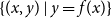


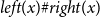
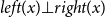


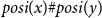


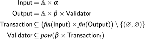


 Open access