


1 Introduction
Private-sector expectations determine the effectiveness of the main conventional monetary policy instrument, that is, the short-term nominal interest rate, in normal times. Moreover, they are key to the transmission of unconventional monetary policy, for example, quantitative easing and forward guidance, when the short-term nominal interest rate is restricted by the zero lower bound. Therefore, managing private-sector expectations has become a primary objective for monetary policy makers.
To influence private-sector expectations, nowadays, central banks provide the public with detailed information about their views of monetary policy and the fundamental factors driving their monetary policy decisions (Blinder et al. (Reference Blinder, Ehrmann, Fratzscher, De Haan and Jansen2008)). A pivotal aspect in this regard is the central bank practice to publish inflation projections. This practice, which qualifies as a tool of “Delphic forward guidance,”Footnote 1 intends to provide superior information about future macroeconomic developments to the private sector and thereby to reduce private-sector uncertainty (Campbell et al. (Reference Campbell, Evans, Fisher, Justiniano, Calomiris and Woodford2012)). But central banks may also use this tool to strategically influence private-sector expectations by intentionally over- or underreporting the projected level of inflation (Gomez-Barrero and Parra-Polania (Reference Gomez-Barrero and Parra-Polania2014); Charemza and Ladley (Reference Charemza and Ladley2016); Jensen (Reference Jensen2016)).
While the publication of central bank inflation projections might be a powerful tool for private-sector expectations management, the central bank must consider its effects on the (endogenous) credibilityFootnote 2 of its future projections (Blinder (Reference Blinder2000)). Publishing accurate inflation projections strengthens the central bank’s reputation as a credible forecaster, but it prevents the central bank from strategically managing private-sector expectations. Conversely, publishing intentionally biased inflation projections may allow the central bank to steer private-sector expectations in the direction necessary to drive inflation closer to the central bank’s inflation target, but it may be damaging to credibility if the published projections result in large forecast errors. This trade-off between short-term gains and potential long-term losses raises the question how the central bank’s ability to manage expectations via inflation projections depends on their credibility and how in turn credibility depends on their past forecasting performance.
Against this background, in this paper we study (i) whether central banks can influence or even manage private-sector expectations via the publication of strategic inflation projections.Footnote 3 If so, (ii) whether such expectations management can be used as an instrument to stabilize inflation and output in normal times and in times of severe economic stress (i.e. periods where there is a high probability of the zero lower bound on the nominal interest rate becoming binding) and (iii) how the effectiveness of such instrument depends on the endogenous degree of the central bank’s credibility as an accurate forecaster.
The analysis is conducted by means of a laboratory experiment.Footnote 4 The great advantage of a laboratory experiment for the questions at hand is that we can control the economic environment in which real human subjects form their expectations. This allows us to clearly identify the impact of publishing strategic central bank inflation projections on the subjects’ expectation formation process and on the resulting dynamic evolution of the underlying theoretical economy. Moreover, studying such policy intervention directly in the field is not possible, since no central bank would risk its reputation by experimenting with untested forms of strategic deception.
The underlying economic environment of the experiment is given by a standard forward-looking New Keynesian model with zero lower bound on the nominal interest rate. The experimental task for the subjects is a learning-to-forecast experiment as pioneered by Marimon and Sunder (Reference Marimon and Sunder1993). Acting in the role of “professional forecasters” in the private sector, subjects are asked repeatedly to form expectations about inflation one period ahead. Prior to submitting their forecast, they are presented with a one-period ahead inflation projection that is published by the central bank. Cornand and Hubert (Reference Cornand and Hubert2020) show that inflation expectations from learning-to-forecast experiments are not fundamentally different from inflation expectations from the field.Footnote 5 We, therefore, are confident that eliciting inflation expectations with a learning-to-forecast experiment has external validity.
We find that the publication of strategic inflation projections strongly affects private-sector expectations. Subjects put a large weight on the public inflation projection when forming their expectations about future inflation. Strategic inflation projections act as a focal point, coordinating expectations by reducing the dispersion and hence the disagreement among individual forecasts. Moreover, they help stabilize the economy; they bring inflation and output faster and closer toward the central bank’s target and reduce their volatility over the business cycle. At the zero lower bound, the publication of overly optimistic strategic projections greatly reduces the risk of deflationary spirals. We show that these results do not solely come from the role of projections as a focal point but also depend on the plausibility of the projections. For instance, if inflation projections are pure noise, they remain without effect for macroeconomic stability. Finally, we show that credibility is an important factor for the stabilizing role of central bank inflation projections. Nevertheless, achieving full credibility on expense of all strategic behavior is not optimal.
Albeit publishing inflation projections is common practice for central banks, it has yet received very little attention in the context of learning-to-forecast experiments. To the best of our knowledge, there are only two exceptions: Mokhtarzadeh and Petersen (Reference Mokhtarzadeh and Petersen2021) and Rholes and Petersen (Reference Rholes and Petersen2021). Mokhtarzadeh and Petersen (Reference Mokhtarzadeh and Petersen2021) study the effects of central bank projections of inflation, the output gap, and the interest rate on expectation formation and economic stability. Rholes and Petersen (Reference Rholes and Petersen2021) study the emerging practice of communicating uncertainty in the central bank’s inflation projections, by comparing the effects of point and density projections by the central bank. In contrast to this paper, projections in these papers abstract from any strategic motive, that is, they are unbiased. Furthermore, they do not study situations when the zero lower bound of the nominal interest rate is binding.
The paper is organized as follows. Section 2 reviews the relevant literature. Section 3 describes our experimental design. Section 4 analyzes the expectation formation processes of the subjects. In Section 5, we study the influence of published central bank inflation projections on economic stability. Section 6 analyzes the interaction of strategic published inflation projections and credibility and discusses how this interaction affects the stabilizing role of published inflation projections. Finally, Section 7 concludes.
2 Related Literature
Laboratory experiments on monetary policy have become increasingly popular in recent years (see Cornand and Heinemann (Reference Cornand, Heinemann and Duffy2014) and Duffy (Reference Duffy, Kagel and Roth2016) for extensive surveys). Pioneering work includes Blinder and Morgan (Reference Blinder and Morgan2005, Reference Blinder and Morgan2008) who compare how interest rate setting decisions are made by individuals, in leaderless groups, and in groups with a designated leader.
A considerable fraction of the literature on monetary policy in laboratory experiments deals with learning-to-forecast experiments in New Keynesian models. Adam (Reference Adam2007) shows that, in such an environment, subjects’ expectation formation processes generally fail to be rational, but can be rather described by simple forecasting rules based on lagged inflation. Pfajfar and Zakelj (Reference Pfajfar and Zakelj2014, Reference Pfajfar and Zakelj2018), Assenza et al. (Reference Assenza, Heemeijer, Hommes and Massaro2021), and Mauersberger (Reference Mauersberger2021) study the expectation formation process of the subjects and its interaction with conventional monetary policy rules. They find a stronger mandate for price stability advances the coordination of private-sector expectations and reduces the volatility of economic fundamentals.Footnote 6 Moreover, it is shown by Hommes, Massaro and Weber (Reference Hommes, Massaro and Weber2019) that both inflation and output gap volatility can further be reduced if the central bank additionally responds to the output gap. Kryvtsov and Petersen (Reference Kryvtsov and Petersen2015) show that much of the stabilizing power of monetary policy is through its effect on private-sector expectations. Close to the zero lower bound, however, Hommes et al. (Reference Hommes, Massaro and Weber2019) find that conventional monetary policy is generally not very effective in stabilizing the economy and cannot reduce the risk of falling into an expectations-driven liquidity trap.
The effects of central bank communication in New Keynesian learning-to-forecast experiments are mixed. While Cornand and M’Baye (Reference Cornand and M’Baye2016, Reference Cornand and M’Baye2018) find that the communication of the central bank’s inflation target can stabilize the economy by reducing volatility in normal times, Arifovic and Petersen (Reference Arifovic and Petersen2017) find that it does not provide a stabilizing anchor in crisis times, for example, in a liquidity trap. Mokhtarzadeh and Petersen (Reference Mokhtarzadeh and Petersen2021) find that providing the economy with central bank projections for inflation and the output gap stabilizes the economy through the coordination of expectations. Related to this, Rholes and Petersen (Reference Rholes and Petersen2021) show that communicating the central bank’s pure point projections of inflation coordinates expectations better than providing additional density projections with the goal to convey a subjective measure of uncertainty associated with these projections. Providing density projections has recently become a common practice among many central banks worldwide. Regarding the communication of interest rates, Kryvtsov and Petersen (Reference Kryvtsov and Petersen2015, Reference Kryvtsov and Petersen2021) and Mokhtarzadeh and Petersen (Reference Mokhtarzadeh and Petersen2021) find that projections of future interest rates cannot consistently stabilize the economy. Yet, Kryvtsov and Petersen (Reference Kryvtsov and Petersen2021) show that communicating the direction of recent interest rate changes stabilizes the economy, because it supports subjects’ understanding of how monetary policy reacts to a given state of the economy.
3 Experimental Design
The experimental design heavily borrows from Assenza et al. (Reference Assenza, Heemeijer, Hommes and Massaro2021). Subjects interact with the economy through expectations of inflation, which affect the contemporaneous outcome of the economy through positive feedbackFootnote 7 of the form:
 \begin{equation}\pi_{t}=f\left(\bar{E_{t}}\pi_{t+1}\right),\end{equation}
where
 $\pi_t$
and
$\pi_t$
and
 $\bar{E_{t}}\pi_{t+1}$
denote inflation and aggregate private-sector expected future inflation, respectively, and f is a functional form, which is specified below. Note that subjects do not yet know the realization of
$\bar{E_{t}}\pi_{t+1}$
denote inflation and aggregate private-sector expected future inflation, respectively, and f is a functional form, which is specified below. Note that subjects do not yet know the realization of
 $\pi_t$
when they form their expectation about
$\pi_t$
when they form their expectation about
 $\pi_{t+1}$
, but have information about the economy only up to period
$\pi_{t+1}$
, but have information about the economy only up to period
 $t-1$
. We follow Kryvtsov and Petersen (Reference Kryvtsov and Petersen2015, Reference Kryvtsov and Petersen2021) and Arifovic and Petersen (Reference Arifovic and Petersen2017) and define aggregate private-sector inflation expectations as the medianFootnote 8 of the individual subjects inflation expectations, that is,
$t-1$
. We follow Kryvtsov and Petersen (Reference Kryvtsov and Petersen2015, Reference Kryvtsov and Petersen2021) and Arifovic and Petersen (Reference Arifovic and Petersen2017) and define aggregate private-sector inflation expectations as the medianFootnote 8 of the individual subjects inflation expectations, that is,
 $\bar{E_{t}}\pi_{t+1}=median(\mathbf{E_{t}\pi_{t+1}})$
, where
$\bar{E_{t}}\pi_{t+1}=median(\mathbf{E_{t}\pi_{t+1}})$
, where
 $\mathbf{E_{t}\pi_{t+1}}$
is a vector collecting all
$\mathbf{E_{t}\pi_{t+1}}$
is a vector collecting all
 $j=1,...J$
subjects’ individual inflation expectations
$j=1,...J$
subjects’ individual inflation expectations
 $E_t^{fc,j}\pi_{t+1}$
of period t for period
$E_t^{fc,j}\pi_{t+1}$
of period t for period
 $t+1$
.
$t+1$
.
3.1 The New Keynesian Economy
The underlying economy evolves according to a New Keynesian model under heterogeneous expectations.Footnote 9
 \begin{equation} y_t=\tilde{E_t}y_{t+1}-\frac{1}{\sigma} \left(r_t-\bar{E_t}\pi_{t+1}-\bar{r}\right)+e_t,\end{equation}
 \begin{equation} \pi_t=\beta \bar{E_t}\pi_{t+1}+\kappa y_t+u_t,\end{equation}
 \begin{equation} r_t=max \left[0,\bar{r}+\pi^T+\phi_\pi \left(\pi_{t}-\pi^T\right)+\phi_y y_{t}\right],\end{equation}
where
 $y_t$
is the aggregate output gap,
$y_t$
is the aggregate output gap,
 $r_t$
is the nominal interest rate,
$r_t$
is the nominal interest rate,
 $\bar{r}=\frac{1}{\beta}-1$
is the steady-state interest rate, and
$\bar{r}=\frac{1}{\beta}-1$
is the steady-state interest rate, and
 $\tilde{E_t}y_{t+1}$
is the aggregate expected future output gap. The parameter
$\tilde{E_t}y_{t+1}$
is the aggregate expected future output gap. The parameter
 $\pi^T$
denotes the central bank’s target value for inflation. In line with, for instance, Assenza et al. (Reference Assenza, Heemeijer, Hommes and Massaro2021), Cornand and M’Baye (Reference Cornand and M’Baye2016, Reference Cornand and M’Baye2018), and Hommes et al. (Reference Hommes, Massaro and Weber2019), the economy is perturbed by stochastic i.i.d. demand and supply shocks with small standard deviation, denoted by
$\pi^T$
denotes the central bank’s target value for inflation. In line with, for instance, Assenza et al. (Reference Assenza, Heemeijer, Hommes and Massaro2021), Cornand and M’Baye (Reference Cornand and M’Baye2016, Reference Cornand and M’Baye2018), and Hommes et al. (Reference Hommes, Massaro and Weber2019), the economy is perturbed by stochastic i.i.d. demand and supply shocks with small standard deviation, denoted by
 $e_t$
and
$e_t$
and
 $u_t$
, respectively.Footnote 10 This is done to let experimental results reflect endogenous dynamics and the expectation formation of subjects rather than external shocks (large highly persistent positive or negative shocks could hinder or facilitate convergence to the target in a—for this study—non-meaningful way). Moreover, for example, Milani (Reference Milani2011) shows that bounded rationality in expectations amplifies persistence endogenously and removes the need for highly persistent fundamental shocks to fit the data. We acknowledge, however, that some of our results may be different if we would, instead, assume auto-correlated shocks as, for instance, in Pfajfar and Zakelj (Reference Pfajfar and Zakelj2014, Reference Pfajfar and Zakelj2018), Mokhtarzadeh and Petersen (Reference Mokhtarzadeh and Petersen2021), or Rholes and Petersen (Reference Rholes and Petersen2021).
$u_t$
, respectively.Footnote 10 This is done to let experimental results reflect endogenous dynamics and the expectation formation of subjects rather than external shocks (large highly persistent positive or negative shocks could hinder or facilitate convergence to the target in a—for this study—non-meaningful way). Moreover, for example, Milani (Reference Milani2011) shows that bounded rationality in expectations amplifies persistence endogenously and removes the need for highly persistent fundamental shocks to fit the data. We acknowledge, however, that some of our results may be different if we would, instead, assume auto-correlated shocks as, for instance, in Pfajfar and Zakelj (Reference Pfajfar and Zakelj2014, Reference Pfajfar and Zakelj2018), Mokhtarzadeh and Petersen (Reference Mokhtarzadeh and Petersen2021), or Rholes and Petersen (Reference Rholes and Petersen2021).
The calibration of the constant model parameters follows Clarida et al. (Reference Clarida, Galí and Gertler2000). We set the quarterly discount factor
 $\beta=0.99$
, implying an annual risk-free interest rate of 4%. The coefficient of relative risk aversion is set to
$\beta=0.99$
, implying an annual risk-free interest rate of 4%. The coefficient of relative risk aversion is set to
 $\sigma=1$
and the output elasticity of inflation is
$\sigma=1$
and the output elasticity of inflation is
 $\kappa=0.3$
. The quarterly inflation target is set to
$\kappa=0.3$
. The quarterly inflation target is set to
 $\pi^T=0.00045$
, implying an annual inflation rate of
$\pi^T=0.00045$
, implying an annual inflation rate of
 $0.18$
%.Footnote 11 The Taylor rule coefficients are chosen to be
$0.18$
%.Footnote 11 The Taylor rule coefficients are chosen to be
 $\phi_\pi=1.25$
and
$\phi_\pi=1.25$
and
 $\phi_y=0.3$
, which is well within the range of values that are common in related experiments.Footnote 12
$\phi_y=0.3$
, which is well within the range of values that are common in related experiments.Footnote 12
Equation (2) refers to an optimized IS curve, equation (3) is the New Keynesian Phillips curve, and equation (4) is the rule for the nominal interest rate set by the central bank. We assume the central bank follows a Taylor (Reference Taylor1993) type interest rate rule, where it adjusts the interest rate in response to inflation and output gap. Furthermore, equation (4) also shows that the nominal interest rate is subject to a zero lower bound.Footnote 13 Under rational expectations this model has two steady states. A locally determinate steady state that has values of inflation and output (close to)
 $\pi_t=y_t=0$
given that
$\pi_t=y_t=0$
given that
 $\pi^T$
is (close to) zero, and a locally indeterminate steady state where the zero lower bound on the nominal interest rate is binding and
$\pi^T$
is (close to) zero, and a locally indeterminate steady state where the zero lower bound on the nominal interest rate is binding and
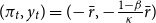 $(\pi_t,y_t)=(\!-\bar{r},-\frac{1-\beta}{\kappa}\bar{r})$
(Benhabib et al. (Reference Benhabib, Schmitt-Grohé and Uribe2001)). Under adaptive learning and other backward-looking expectation formation processes the target steady state is locally stable (if the Taylor principle is satisfied), while the zero lower bound steady state is an unstable saddle point (see, e.g., Evans et al. (Reference Evans, Guse and Honkapohja2008); Hommes and Lustenhouwer (Reference Hommes and Lustenhouwer2019); and Lustenhouwer (Reference Lustenhouwer2021)). Therefore, depending on initial conditions, either convergence to the target steady state occurs or the economy falls into a deflationary spiral (Evans et al. (Reference Evans, Guse and Honkapohja2008)).
$(\pi_t,y_t)=(\!-\bar{r},-\frac{1-\beta}{\kappa}\bar{r})$
(Benhabib et al. (Reference Benhabib, Schmitt-Grohé and Uribe2001)). Under adaptive learning and other backward-looking expectation formation processes the target steady state is locally stable (if the Taylor principle is satisfied), while the zero lower bound steady state is an unstable saddle point (see, e.g., Evans et al. (Reference Evans, Guse and Honkapohja2008); Hommes and Lustenhouwer (Reference Hommes and Lustenhouwer2019); and Lustenhouwer (Reference Lustenhouwer2021)). Therefore, depending on initial conditions, either convergence to the target steady state occurs or the economy falls into a deflationary spiral (Evans et al. (Reference Evans, Guse and Honkapohja2008)).
Finally, aggregate output gap expectations
 $\tilde{E_t}{y_{t+1}}$
are endogenously determined by the model.
$\tilde{E_t}{y_{t+1}}$
are endogenously determined by the model.
 $\tilde{E}(y)$
follows a Heuristic Switching Model (Brock and Hommes (Reference Brock and Hommes1997)) that was originally developed to fit a learning-to-forecast experiment in an asset price setting (Anufriev and Hommes (Reference Anufriev and Hommes2012)) but has proven its robustness to fit also learning-to-forecast experiments in New Keynesian frameworks (e.g. Assenza et al. (Reference Assenza, Heemeijer, Hommes and Massaro2021)). The Heuristic Switching Model can be summarized by the following equations:
$\tilde{E}(y)$
follows a Heuristic Switching Model (Brock and Hommes (Reference Brock and Hommes1997)) that was originally developed to fit a learning-to-forecast experiment in an asset price setting (Anufriev and Hommes (Reference Anufriev and Hommes2012)) but has proven its robustness to fit also learning-to-forecast experiments in New Keynesian frameworks (e.g. Assenza et al. (Reference Assenza, Heemeijer, Hommes and Massaro2021)). The Heuristic Switching Model can be summarized by the following equations:
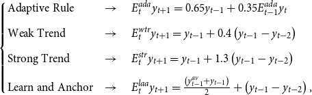 \begin{equation} \begin{cases} \mbox{Adaptive Rule} & \rightarrow \quad E^{ada}_ty_{t+1}=0.65y_{t-1}+0.35E^{ada}_{t-1}y_t\\ \\[-6pt] \mbox{Weak Trend }& \rightarrow \quad E^{wtr}_ty_{t+1}=y_{t-1}+0.4\left(y_{t-1}-y_{t-2}\right)\\ \\[-6pt] \mbox{Strong Trend } &\rightarrow \quad E^{str}_ty_{t+1}=y_{t-1}+1.3\left(y_{t-1}-y_{t-2}\right)\\ \\[-6pt] \mbox{Learn and Anchor}& \rightarrow \quad E^{laa}_ty_{t+1}=\frac{\left(y^{av}_{t-1}+y_{t-1}\right)}{2}+\left(y_{t-1}-y_{t-2}\right), \end{cases}\end{equation}
 \begin{equation} U^h_{t-1}=\frac{100}{1+\vert y_{t-1}-E^h_{t-2}y_{t-1}\vert}+\eta U^h_{t-2},\end{equation}
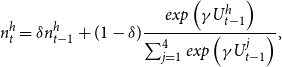 \begin{equation} n^h_{t}=\delta n^h_{t-1}+(1-\delta)\frac{exp\left(\gamma U^h_{t-1}\right)}{\sum\nolimits_{j=1}^4 exp\left(\gamma U^j_{t-1}\right)},\end{equation}
 \begin{equation} \tilde{E_t} y_{t+1} =E^{ada}_ty_{t+1}n_t^{ada}+E^{wtr}_ty_{t+1}n_t^{wtr}+E^{str}_ty_{t+1}n_t^{str}+E^{laa}_ty_{t+1}n_t^{laa}.\end{equation}
Equation (5) lists the set of forecast heuristics. The variable
 $y^{av}_{t-1}$
denotes the average past output gap. Once heuristics are used, the agents weight their past performance following equation (6), with
$y^{av}_{t-1}$
denotes the average past output gap. Once heuristics are used, the agents weight their past performance following equation (6), with
 $\eta$
denoting the parameter describing the preference for the past. Equation (7) updates the probability of using heuristic h when forecasting for period
$\eta$
denoting the parameter describing the preference for the past. Equation (7) updates the probability of using heuristic h when forecasting for period
 $t+1$
. Notice that
$t+1$
. Notice that
 $\gamma$
captures the sensitivity of agents to heuristic performances and
$\gamma$
captures the sensitivity of agents to heuristic performances and
 $\delta$
denotes the fraction of agents that in period t stick to the heuristic they used in period
$\delta$
denotes the fraction of agents that in period t stick to the heuristic they used in period
 $t-1$
. Then, using (8), the expectation is aggregated and
$t-1$
. Then, using (8), the expectation is aggregated and
 $\tilde{E_t}y_{t+1}$
is determined. The calibration of the Heuristic Switching Model follows Assenza et al. (Reference Assenza, Heemeijer, Hommes and Massaro2021), that is, we set
$\tilde{E_t}y_{t+1}$
is determined. The calibration of the Heuristic Switching Model follows Assenza et al. (Reference Assenza, Heemeijer, Hommes and Massaro2021), that is, we set
 $\eta = 0.7$
and
$\eta = 0.7$
and
 $\delta = 0.9$
. Because we let the Heuristic Switching Model work with quarterly rather than annualized output data, we calibrate the intensity of choice higher than Assenza et al. (Reference Assenza, Heemeijer, Hommes and Massaro2021) and set it at
$\delta = 0.9$
. Because we let the Heuristic Switching Model work with quarterly rather than annualized output data, we calibrate the intensity of choice higher than Assenza et al. (Reference Assenza, Heemeijer, Hommes and Massaro2021) and set it at
 $\gamma = 6.4$
. For this calibration of the intensity of choice, we get sensible switching dynamics, qualitatively in line with those in Assenza et al. (Reference Assenza, Heemeijer, Hommes and Massaro2021).
$\gamma = 6.4$
. For this calibration of the intensity of choice, we get sensible switching dynamics, qualitatively in line with those in Assenza et al. (Reference Assenza, Heemeijer, Hommes and Massaro2021).
3.2 The Experiment
We apply a learning-to-forecast experiment following the approach of Assenza et al. (Reference Assenza, Heemeijer, Hommes and Massaro2021). The general setup is as follows: the experiment has a total of 37 periods which are divided into a preliminary stage (periods 1–8) and a main stage (periods 9–37). Subjects in the laboratory are randomly divided into groups of 7. In the main stage of the experiment, subjects take the role of either a professional forecaster or a central bank forecaster. Professional forecasters are employed at the forecasting department of a company which needs predictions about future inflation as input for the management’s operative decisions. Professional forecasters’ job is to generate these inflation forecasts and to communicate them to the management. Professional forecasters are provided with some qualitative knowledge of the economyFootnote 14 and the direction of the feedback on their expectations (i.e. positive feedback). With the exception of the control treatment, professional forecasters are also presented with a public central bank projection. The professional forecasters’ payoffs are determined according to their forecasting performance, measured by the following payoff function from Assenza et al. (Reference Assenza, Heemeijer, Hommes and Massaro2021):
 \begin{equation} \Pi_{fc,j}=\frac{100}{1+|\pi_{t+1}-E_t^{fc,j}\pi_{t+1}|}.\end{equation}
The central bank forecaster is employed at the forecasting department of the central bank and the central bank forecaster’s job, too, is to generate inflation forecasts, which we denote
 $E_t^{cbf}\pi_{t+1}$
. However, this forecast does not enter the vector
$E_t^{cbf}\pi_{t+1}$
. However, this forecast does not enter the vector
 $\mathbf{E_{t}\pi_{t+1}}$
from which the aggregate inflation expectation is determined. The incentives for the central bank forecaster in determining her inflation forecasts, therefore, are different from the incentives of professional forecasters and also differ strongly between treatments. These differences will be explained in Section 3.4.
$\mathbf{E_{t}\pi_{t+1}}$
from which the aggregate inflation expectation is determined. The incentives for the central bank forecaster in determining her inflation forecasts, therefore, are different from the incentives of professional forecasters and also differ strongly between treatments. These differences will be explained in Section 3.4.
Whether a subject is assigned the role of a professional forecaster or a central bank forecaster is the outcome of the preliminary stage (henceforth: Stage I). In Stage I, all subjects of a group (including the subject that will later turn out to be chosen as central banker) play 8 initial rounds of the experiment (periods 1–8) as professional forecasters, in the absence of any public central bank inflation projection. To level the playing field, all participating subjects are presented with an identical pre-determined three-period history (for periods
 $t=-2$
,
$t=-2$
,
 $t=-1$
, and
$t=-1$
, and
 $t=0$
) for inflation, the output gap, and the interest rate, which initializes the economy away from the central bank’s target values.Footnote 15 At the end of the 8 initial rounds, subjects are ranked according to their relative forecasting performance in Stage I. The role of the central bank forecaster for the remaining rounds of the experiment (periods 9–37) is assigned to the best ranked subject, and this is common knowledge. This selection mechanism is very similar to the one used to select leaders of monetary policy committees in the experiment of Blinder and Morgan (Reference Blinder and Morgan2008).
$t=0$
) for inflation, the output gap, and the interest rate, which initializes the economy away from the central bank’s target values.Footnote 15 At the end of the 8 initial rounds, subjects are ranked according to their relative forecasting performance in Stage I. The role of the central bank forecaster for the remaining rounds of the experiment (periods 9–37) is assigned to the best ranked subject, and this is common knowledge. This selection mechanism is very similar to the one used to select leaders of monetary policy committees in the experiment of Blinder and Morgan (Reference Blinder and Morgan2008).
Ideally, we would like to employ a representative sample of households, firms, and financial market professionals in the role of the professional forecasters and professional central bankers in the role of the central bank forecaster. Yet, previous experimental evidence makes us believe that our results derived from inexperienced student subjects have external validity and are relevant for the discussion about the conduct of monetary policy. Foremost, Cornand and Hubert (Reference Cornand and Hubert2020) show that inflation expectations elicited from learning-to-forecast experiments share important patterns and characteristics with inflation expectations elicited from surveys (such as the Michigan Survey of Consumer Attitudes and Behavior, the Livingston Survey, and the Survey of Professional Forecasters) and inflation expectations extracted from financial instruments such as inflation swaps. Furthermore, Arifovic and Sargent (Reference Arifovic, Sargent, Altig and Smith2003), Engle-Warnick and Turdaliev (Reference Engle-Warnick and Turdaliev2010), and Duffy and Heinemann (Reference Duffy and Heinemann2021) put student subjects in the role of central bankers and show that they perform reasonably well, even in such complex and uncommon decision-making processes.Footnote 16
Since we are interested in the expectations channel of monetary policy both in normal times and in times when the zero lower bound on the nominal interest rate may become binding, in the spirit of Arifovic and Petersen (Reference Arifovic and Petersen2017), starting in period 29 there is a series of four consecutive negative demand shocks. The shocks are chosen such that the forced recession is likely to drive the economy into the liquidity trap and therewith the possibility of a deflationary spiral. With this subdivision, the economy is fairly stable in the first part of the actual experiment (periods 9–28; henceforth: Stage II). Here it is investigated whether published central bank inflation projections can influence private-sector expectations and actively stabilize the economy. In the latter part of the experiment (periods 29–37; henceforth: Stage III), on the other hand, it is investigated whether the central bank can prevent or reverse a deflationary spiral with its published inflation projections.
The timing of the experiment is as follows: In
 $t=1,...,8$
(Stage I), all subjects submit their inflation forecast
$t=1,...,8$
(Stage I), all subjects submit their inflation forecast
 $E_t^{fc,j}\pi_{t+1}$
simultaneously. In
$E_t^{fc,j}\pi_{t+1}$
simultaneously. In
 $t=9,...,37$
(Stages II and III), first the central bank forecaster submits her forecast
$t=9,...,37$
(Stages II and III), first the central bank forecaster submits her forecast
 $E_t^{cbf}\pi_{t+1}$
. Professional forecasters observe the public projection
$E_t^{cbf}\pi_{t+1}$
. Professional forecasters observe the public projection
 $E_{t}^{pub} \pi_{t+1}$
and subsequently submit their own forecasts
$E_{t}^{pub} \pi_{t+1}$
and subsequently submit their own forecasts
 $E_{t}^{fc} \pi_{t+1}$
. After all professional forecasters have submit their forecast, the aggregate inflation forecast, which we denote as
$E_{t}^{fc} \pi_{t+1}$
. After all professional forecasters have submit their forecast, the aggregate inflation forecast, which we denote as
 $\bar{E_t}\pi_{t+1}$
, is determined, and the values for the variables in period t are computed. The economy proceeds to the next round.
$\bar{E_t}\pi_{t+1}$
, is determined, and the values for the variables in period t are computed. The economy proceeds to the next round.
3.3 The Central Bank Inflation Projection
In each period, the central bank forecasting department generates an inflation projection. To do so, it is provided with superior information about the experimental economy.
First, the central bank is provided with a data-driven forecast
 $E_{t}^{ddf} \pi_{t+1}$
. The data-driven forecast uses all data up to period
$E_{t}^{ddf} \pi_{t+1}$
. The data-driven forecast uses all data up to period
 $t-1$
, as well as detailed knowledge of the model, to predict what level of inflation is expected to prevail in period
$t-1$
, as well as detailed knowledge of the model, to predict what level of inflation is expected to prevail in period
 $t+1$
. In particular, complete knowledge of the New Keynesian model equations (2) to (4) is used here, including the parameter values. Second, the data-driven forecast is able to perfectly predict how output expectations will be formed using the Heuristic Switching Model that describes output gap expectations in the economy (equations (5) to (8)). The only unknowns, therefore, are inflation expectations and future shock realizations. For future shock realizations, their expected values of zero are used. To make accurate predictions on current and future private-sector inflation expectations, these expectations need to be modeled. For this, we use an analogue Heuristic Switching Model for output expectations. As mentioned above, this model has proven to fit learning-to-forecast expectations in similar frameworks well. To account for the potential self-fulfilling properties that a published central bank projection can have on the economy,Footnote 17 the Heuristic Switching Model for inflation is extended with a fifth heuristic. This heuristic is termed “Follow the Published Projection” and is defined as
$t+1$
. In particular, complete knowledge of the New Keynesian model equations (2) to (4) is used here, including the parameter values. Second, the data-driven forecast is able to perfectly predict how output expectations will be formed using the Heuristic Switching Model that describes output gap expectations in the economy (equations (5) to (8)). The only unknowns, therefore, are inflation expectations and future shock realizations. For future shock realizations, their expected values of zero are used. To make accurate predictions on current and future private-sector inflation expectations, these expectations need to be modeled. For this, we use an analogue Heuristic Switching Model for output expectations. As mentioned above, this model has proven to fit learning-to-forecast expectations in similar frameworks well. To account for the potential self-fulfilling properties that a published central bank projection can have on the economy,Footnote 17 the Heuristic Switching Model for inflation is extended with a fifth heuristic. This heuristic is termed “Follow the Published Projection” and is defined as
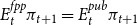 $E^{fpp}_t\pi_{t+1}=E^{pub}_t\pi_{t+1}$
. That is, the Heuristic Switching Model of inflation expectations captures that more professional forecasters will form their expectations in line with the published projection when this published projected has made accurate forecasts relative to other forecasting heuristics in the (recent) past.
$E^{fpp}_t\pi_{t+1}=E^{pub}_t\pi_{t+1}$
. That is, the Heuristic Switching Model of inflation expectations captures that more professional forecasters will form their expectations in line with the published projection when this published projected has made accurate forecasts relative to other forecasting heuristics in the (recent) past.
Note that, in the control treatment, there is no published forecast, and the “Follow the Published Projection” heuristic is excluded from the model of inflation expectation. For that case, it is straightforward to calculate the expected value of future inflation, given knowledge of the model equations and past data and given the model of inflation expectations. In that treatment, the data-driven forecast is equal to this expected value. In the other treatments, the published projection affects modeled inflation expectations and hence the expected value of future inflation. What can be calculated here, is the expected value of future inflation, given a particular published projection.Footnote 18 For different published projections, the resulting expected value of future inflation may be close to, or far away from, the published projection. By calculating this expected value for a wide range of possible published projections and performing a grid search, we can identify the published projection that is equal (or as close as possible) to the implied expected value of future inflation. When the central bank published this projection, it is most likely that next period’s realized inflation will be equal to the projection. This value is, therefore, taken as the data-driven forecast in treatments where a central bank projection is published.
Next, the central bank is provided with information about which aggregate inflation expectations for the following period would need to prevail for inflation to jump (in expectations) immediately to the target level
 $\pi^T$
. This specific aggregate inflation expectation is calculated by performing a grid search on
$\pi^T$
. This specific aggregate inflation expectation is calculated by performing a grid search on
 $\bar{E}_t\pi_{t+1}$
in the model defined by equations (2) to (8). This information tells the central bank in what direction it should steer aggregate inflation expectations about
$\bar{E}_t\pi_{t+1}$
in the model defined by equations (2) to (8). This information tells the central bank in what direction it should steer aggregate inflation expectations about
 $t+1$
to get closer to its inflation target in period t. We label this piece of information “required for target” and denote it by
$t+1$
to get closer to its inflation target in period t. We label this piece of information “required for target” and denote it by
 $E_t^{rft}\pi_{t+1}$
.
$E_t^{rft}\pi_{t+1}$
.
Finally, the central bank is presented with a “credibility index” measuring aggregate credibility given to the central bank projections by the individual professional forecasters from the recent past. In the spirit of Cecchetti and Krause (Reference Cecchetti and Krause2002), we base our measure of the central bank’s credibility toward a professional forecaster j by the distance between the central bank’s inflation projection and j’s inflation forecast. We normalize this distance such that
 $Cred_{t}^{j}$
takes values between 0 (projection is not credible at all) and 1 (projection fully credible). Hence, individual credibility is given by
$Cred_{t}^{j}$
takes values between 0 (projection is not credible at all) and 1 (projection fully credible). Hence, individual credibility is given by
 \begin{equation}Cred_{t}^{j}= exp\left(\!-3 \cdot \left(E_{t}^{pub}\pi_{t+1}-E_{t}^{fc,j}\pi_{t+1}\right)^2\right).\end{equation}
The scale parameter 3 is calibrated based on pilot data such that deviations from mean credibility of more than one standard deviation result in a zero payoff. The “credibility index” provided to the central bank forecaster is defined as the average credibility given to the central bank by all professional forecasters in the last four periods, that is,
 $I_{t}^{cred}=\frac{1}{24}\sum_{j=1}^{6}\sum_{i=1}^{4} Cred_{t-i}^{j}$
.
$I_{t}^{cred}=\frac{1}{24}\sum_{j=1}^{6}\sum_{i=1}^{4} Cred_{t-i}^{j}$
.
 $I_{t}^{cred}=1$
if all individual forecasts from the last four periods met the central bank projection, and
$I_{t}^{cred}=1$
if all individual forecasts from the last four periods met the central bank projection, and
 $I_{t}^{cred}$
goes to 0 if all forecasts moved infinitely far away from it.
$I_{t}^{cred}$
goes to 0 if all forecasts moved infinitely far away from it.
The data-driven forecast and the “required for target” define an interval of generally sensible inflation projections. If the central bank wants to build up credibility, it follows the data-driven forecast and provides a “non-strategic” inflation projection. If the central bank intends to steer the economy, it provides a “strategic” projection which lies between the data-driven forecast and the “required for target” criterion. The extent to which the inflation projections are biased away from the data-driven forecast and toward the “required for target” criterion determines the degree of strategic-ness.Footnote 19 Inflation projections outside of this interval are not sensible. We term the latter “random” projections.
To sum up, when generating the inflation projection, the central bank must decide whether it follows the data-driven forecast or to what extent it publishes a projection which is biased toward the “required for target” criterion, taking into account its credibility.
3.4 Treatments
We consider four treatments in this experiment.
3.4.1 Treatment 1: No published central bank inflation projections (control treatment)
In this treatment, the control treatment, no central bank projections are published. The central bank forecaster produces forecasts, but these forecasts are not revealed. For her predictions, she is paid according to equation (9).
3.4.2 Treatment 2: Inflation projections from a human central bank forecaster
In this treatment, the central bank publishes official central bank inflation projections (i.e.
 $E_t^{pub}\pi_{t+1}=E_t^{cbf}\pi_{t+1}$
) which are generated by the central bank forecaster subject. The other subjects of her group are informed (i) that there is a central bank forecaster publishing official central bank inflation projections in this economy, (ii) that the central bank forecaster is the subject that predicted inflation best in Stage I, (iii) that the central bank forecaster has additional information about the economy without specifying this any further, and (iv) that the central bank has an inflation target without quantifying this target.Footnote 20 Note that it is not a priori clear whether it is optimal for professional forecasters to use the published projection when forming their own forecasts or to ignore it. This depends on what a subject believes about how the central bank forms its projection and about how other subjects form their expectations.Footnote 21
$E_t^{pub}\pi_{t+1}=E_t^{cbf}\pi_{t+1}$
) which are generated by the central bank forecaster subject. The other subjects of her group are informed (i) that there is a central bank forecaster publishing official central bank inflation projections in this economy, (ii) that the central bank forecaster is the subject that predicted inflation best in Stage I, (iii) that the central bank forecaster has additional information about the economy without specifying this any further, and (iv) that the central bank has an inflation target without quantifying this target.Footnote 20 Note that it is not a priori clear whether it is optimal for professional forecasters to use the published projection when forming their own forecasts or to ignore it. This depends on what a subject believes about how the central bank forms its projection and about how other subjects form their expectations.Footnote 21
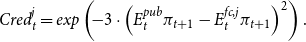
The central bank forecaster’s objective, in this treatment, is twofold: On the one hand, she has to stabilize inflation, that is, minimize the deviations of inflation from her target values, while on the other hand, her inflation projections have to remain maximally credible, as measured by the credibility index. We consider central bank credibility explicitly, as it is of utmost importance for the functioning of monetary policy and thereby enjoys a lot of attention of monetary policy makers (Blinder (Reference Blinder2000); Bordo and Siklos (Reference Bordo and Siklos2014)). In line with this strategy, Gomez-Barrero and Parra-Polania (Reference Gomez-Barrero and Parra-Polania2014) present a theoretical model of strategic central bank forecasting which explicitly considers reputational concerns of central bank credibility in the central bank’s loss function. The payoff functions of the central bank forecaster have the following form:
 \begin{equation} \begin{array}{lll} \Pi_{cbf}^{stability}&=&\max\left(0,100-44.4\left(\pi_t-\pi^T\right)^2\right),\\ \\[-9pt] \Pi_{cbf}^{credibility}&=&\max\left(0,100-400\left(1-I_{t}^{cred}\right)^2\right). \end{array}\end{equation}
Equation (11) is calibrated such that in each period the central bank forecaster receives a payoff of zero for stability if inflation deviates from target by more than 1.5 percentage points and receives a payoff of zero for credibility of the projection if the credibility index is below 0.5. To prevent hedging between the two goals, at the end of the experiment, only one of them is chosen randomly by the computer for payoff (Blanco et al. (Reference Blanco, Engelmann, Koch and Normann2010)).
3.4.3 Treatment 3: “Algorithmic” inflation projections
In this treatment, we follow Mokhtarzadeh and Petersen (Reference Mokhtarzadeh and Petersen2021) and provide a published central bank projection that comes from a computer algorithm. Analogous to the previous treatment, the subjects are informed (i) that there is a computer algorithm publishing official central bank inflation projections in this economy, (ii) that the central bank forecaster has additional information about the economy without specifying this any further, (iii) that it may or may not exploit this superior information, and (iv) that the central bank has an inflation target without quantifying this target.
In contrast to the algorithm proposed by Mokhtarzadeh and Petersen (Reference Mokhtarzadeh and Petersen2021), our computer algorithm makes strategic inflation projections. The extent to which the projections are strategic depends primarily on the current state of the economy (in particular, whether previous inflation was (i) close to, (ii) above, or (iii) below its target value) and secondarily on the credibility of recent central bank inflation projections.
The computer algorithm works as follows: (i) If previous inflation was close to target (within
 $\pm0.5$
percentage points), the central bank tries to initiate long-term coordination on its inflation target through projections equal to the inflation target. (ii) If previous inflation was sufficiently above target (for more than
$\pm0.5$
percentage points), the central bank tries to initiate long-term coordination on its inflation target through projections equal to the inflation target. (ii) If previous inflation was sufficiently above target (for more than
 $0.5$
percentage points), the algorithm solves a trade-off between building credibility and steering the economy. If past projections have been little credible, the algorithm aims at building credibility through accurate inflation projections based primarily on the data-driven forecast (which is calculated in the same way as in Treatment 2). If projections have been credible, the algorithm leans more toward the “required-for-target” information. (iii) If previous inflation was sufficiently below target (for more than
$0.5$
percentage points), the algorithm solves a trade-off between building credibility and steering the economy. If past projections have been little credible, the algorithm aims at building credibility through accurate inflation projections based primarily on the data-driven forecast (which is calculated in the same way as in Treatment 2). If projections have been credible, the algorithm leans more toward the “required-for-target” information. (iii) If previous inflation was sufficiently below target (for more than
 $0.5$
percentage points), the economy faces the risk of a binding zero lower bound and a deflationary spiral. Now, building up credibility by following the data-driven forecast becomes dangerous as the data-driven forecast may predict a deflationary spiral. Therefore, the algorithm balances forecasting the target with forecasting the last observed inflation level, where the latter can improve on credibility without amplifying the downturn in inflation. The weight on the last observed value is relatively high when there is a downward trend in inflation, because then it might not be credible that inflation will suddenly go up by much. On the other hand, if there is an upward trend in inflation it might be more credible that inflation will go up more, so the computer algorithm can put more weight on the target.
$0.5$
percentage points), the economy faces the risk of a binding zero lower bound and a deflationary spiral. Now, building up credibility by following the data-driven forecast becomes dangerous as the data-driven forecast may predict a deflationary spiral. Therefore, the algorithm balances forecasting the target with forecasting the last observed inflation level, where the latter can improve on credibility without amplifying the downturn in inflation. The weight on the last observed value is relatively high when there is a downward trend in inflation, because then it might not be credible that inflation will suddenly go up by much. On the other hand, if there is an upward trend in inflation it might be more credible that inflation will go up more, so the computer algorithm can put more weight on the target.
The explicit algorithm is spelled out below:
“close to target”:
 $E^{pub}_t\pi_{t+1}=\pi^T$
“sufficiently above target”:
 $E^{pub}_t\pi_{t+1}= I_{t}^{cred} * E_{t}^{rft} \pi_{t+1} + (1-I_{t}^{cred})E_{t}^{ddf}\pi_{t+1}$
“sufficiently below target”: if
 $\pi_{t-1}<\pi_{t-2}: E^{pub}_t\pi_{t+1}=0.5 \pi^T+ 0.5 \pi_{t-1}$
if
 $\pi_{t-1}>\pi_{t-2}: E^{pub}_t\pi_{t+1}=0.8 \pi^T+ 0.2 \pi_{t-1}$
For reasons of comparability, in this treatment, the central bank forecaster subject takes the same role as in Treatment 1 and is, again, paid for her prediction accuracy according to equation (9).
3.4.4 Treatment 4: “Random” inflation projections
In Stage II of this treatment, the published inflation projections are randomly drawn from a uniform distribution with support from –5 to 5, that is,
 $E^{pub}_t\pi_{t+1}\sim Unif(\!-5,5)$
. The support is chosen according to realized inflation throughout the first three treatments of this experiment. This approach has similarities with the zero-intelligence traders and near-zero-intelligence traders that have been applied to experimental asset market settings (see, e.g., Gode and Sunder (Reference Gode and Sunder1993); Duffy and Ünver (Reference Duffy and U. Ünver2006)). In both cases, decisions are made by random draws, potentially under some small amount of structure. An important difference with that literature is that our random published projections are shown to subjects but do not directly affect the outcomes of the economy, whereas (near-)zero-intelligence traders directly participate in the markets.
$E^{pub}_t\pi_{t+1}\sim Unif(\!-5,5)$
. The support is chosen according to realized inflation throughout the first three treatments of this experiment. This approach has similarities with the zero-intelligence traders and near-zero-intelligence traders that have been applied to experimental asset market settings (see, e.g., Gode and Sunder (Reference Gode and Sunder1993); Duffy and Ünver (Reference Duffy and U. Ünver2006)). In both cases, decisions are made by random draws, potentially under some small amount of structure. An important difference with that literature is that our random published projections are shown to subjects but do not directly affect the outcomes of the economy, whereas (near-)zero-intelligence traders directly participate in the markets.
In Stage III of this treatment, the algorithmic forecast from Treatment 3 is applied. This twist after Stage II allows us to draw conclusions about the persistence of central bank credibility in the light of drastic changes in the economic environment.
3.5 Hypotheses
Our experimental design allows us to address several hypothesis, following the distinction between “strategic” and “random” projections defined in Section 3.3. We consider central bank inflation projections to be strategic, if they lie systematically (i.e. most of the time) inside the interval between the data-driven forecast and the “required for target” information. Analogously, central bank projections are considered “random,” if they lie systematically (i.e. most of the time) outside the interval between the data-driven forecast and the “required for target” information. According to this criterion, projections from a human central bank forecaster and the algorithmic projections are considered “strategic,” while the random projections are indeed considered “random”.Footnote 22
Hypothesis 1: Strategic projections coordinate private-sector inflation expectations by reducing the disagreement (i.e. dispersion) amongst private-sector forecasts; random projections do not.
In their seminal theoretical contribution, Morris and Shin (Reference Morris and Shin2002) show that public central bank information can act as a coordination device that reduces the dispersion of private-sector expectations. Empirical support for such an coordinating effect (especially in the context of public central bank projections) is given by Hubert (Reference Hubert2014) for the Federal Reserve, by Fujiwara (Reference Fujiwara2005) for the Bank of Japan, and by Ehrmann et al. (Reference Ehrmann, Eijffinger and Fratzscher2012) for 12 advanced economies (including the former two).
Hypothesis 2: Strategic projections stabilize the economy (a) in normal times and (b) in times of severe economic stress; random projections do not.
Although from an empirical point of view published central bank inflation projections seem beneficial for macroeconomic stability (Chortareas et al. (Reference Chortareas, Stasavage and Sterne2002)), from a theoretical point of view, the effects of published central bank inflation projections on macroeconomic stability are generally ambiguous and depend on the quality of the projections. Providing superior information, central bank projections can be stabilizing, for example, through a coordinating effect on private sector inflation expectations on a desired path, in normal times (Eusepi and Preston (Reference Eusepi and Preston2010); Ferrero and Secchi (Reference Ferrero and Secchi2010)) and at the zero lower bound (Goy et al. (Reference Goy, Hommes and Mavromatis2020)). By contrast, central bank projections can be destabilizing if potentially noisy projections crowd out more accurate private information (Geraats (Reference Geraats2002); Amato and Shin (Reference Amato and Shin2006); Walsh (Reference Walsh2007)).
Hypothesis 3: The ability of the central bank to stabilize the economy by means of its projections depends positively on the credibility of the central bank projections.
Svensson (Reference Svensson2015) shows for Sweden that credible interest rate projections remarkably influenced market behavior toward stabilization in 2009, whereas in 2011 non-credible projections left the market unimpressed and without any response in market behavior. Moreover, Cole and Martínez-García (Reference Cole and Martnez-Garca2021) show in a model with heterogeneous expectations that the effectiveness of central bank announcements depends on the fraction of agents that take the announcement into account. Using Bayesian methods, they estimate this channel of imperfect credibility to have quantitative importance.
Hypothesis 4: The credibility of the central bank projections depends positively on their past performance
In a survey among 84 central bank presidents worldwide, Blinder (Reference Blinder2000) finds that the most important matter for credibility is believed to be a consistent track record. With respect to inflation projections and projection of inflation in particular, such a consistent track record is established primarily by a sustained projection accuracy. Loss in credibility of the central bank’s projections can therefore be attributed to a (systematic) failure to produce accurate projections (Mishkin (Reference Mishkin, Kent and Guttmann2004)). Following this line of reasoning, also Mokhtarzadeh and Petersen (Reference Mokhtarzadeh and Petersen2021) determine central bank credibility by looking at past central bank forecasting performance.
3.6 Experimental Procedure
Each treatment of this experiment consists of six economies with seven subjects each. Thus, the experiment has a total of
 $4\ \times\ 6\ \times\ 7\,=\,168$
subjects. Subjects were recruited from a variety of academic backgrounds using ORSEE (Greiner (Reference Greiner2015)). The subject population comprised undergraduate students (64%), graduate students (34%), and nonstudents (2%). Subjects were mostly from the natural sciences (61%) and the social sciences (16%). Around two-thirds of the subjects were male (62%) and one-third were female (38%). During the experiment, subjects earned experimental currency units (ECU) according to their respective payoff functions. At the end of the experiment, subjects were paid
$4\ \times\ 6\ \times\ 7\,=\,168$
subjects. Subjects were recruited from a variety of academic backgrounds using ORSEE (Greiner (Reference Greiner2015)). The subject population comprised undergraduate students (64%), graduate students (34%), and nonstudents (2%). Subjects were mostly from the natural sciences (61%) and the social sciences (16%). Around two-thirds of the subjects were male (62%) and one-third were female (38%). During the experiment, subjects earned experimental currency units (ECU) according to their respective payoff functions. At the end of the experiment, subjects were paid
 $\unicode{x20AC}$
1 for every 85 ECU; that is, each ECU paid approximately
$\unicode{x20AC}$
1 for every 85 ECU; that is, each ECU paid approximately
 ${\unicode{x20AC}}$
0.012. The average payment was
${\unicode{x20AC}}$
0.012. The average payment was
 ${\unicode{x20AC}}$
31.66. The experimental software was programmed in oTree (Chen et al. (Reference Chen, Schonger and Wickens2016)). The experiment was conducted in May and June 2016 at the experimental lab of the Technische Universität Berlin.
${\unicode{x20AC}}$
31.66. The experimental software was programmed in oTree (Chen et al. (Reference Chen, Schonger and Wickens2016)). The experiment was conducted in May and June 2016 at the experimental lab of the Technische Universität Berlin.
4 Expectation Formation of Professional Forecasters
For central bank projections to be an effective tool of monetary policy, they must influence the expectation formation process of the professional forecasters. Therefore, in this section we investigate if professional forecasters form expectations differently when presented with central bank projections and if so, how this depends on the quality of the projections. Since Stage I is a learning stage in all treatments and Stage III presents subjects with an inherently unstable environment, we focus this analysis on Stage II only.
We follow Pfajfar and Zakelj (Reference Pfajfar and Zakelj2014) and Assenza et al. (Reference Assenza, Heemeijer, Hommes and Massaro2021) and estimate for each subject’s inflation forecast a general linear forecasting rule of the form
 \begin{equation} E_t^{fc,j}\pi_{t+1}=c^j+\sum_{i=1}^2 \alpha_{i}^j E_{t-i}^{fc,j}\pi_{t+1-i}+\sum_{i=1}^2 \beta_{i}^j \pi_{t-i}+ \gamma^j y_{t-1}+\delta^j E_{t}^{pub}\pi_{t+1}+\varepsilon^j_t,\end{equation}
where
 $\varepsilon^j$
is the error term of each individual regression, using non-linear least squares. For Treatment 1,
$\varepsilon^j$
is the error term of each individual regression, using non-linear least squares. For Treatment 1,
 $\delta^j$
is set equal to zero. The results are summarized in Table 1. The table shows the percentage of individually significant regressors at the 10%-significance level and the median estimated parameter values for each treatment, respectively.Footnote 23 First, we consider all professional forecasters who did not see a central bank projection before making their forecasts. This group consists of all professional forecasters in Treatment 1 (the control treatment). Column [1] of Table 1 shows that 92% of subjects consider the first lag of inflation when forming their expectation about future inflation. 36% of subjects consider the second lag of inflation. Given that the sign of the coefficient on the first lag is generally positive with a median of 1.11, while the sign on the second lag of inflation is generally negative with median of –1.14 it appears that many professional forecasters engaged either in naive adaptive or in trend following behavior when forecasting inflation. In line with early evidence from Adam (Reference Adam2007), only few subjects consider past realizations of the output gap to predict future inflation.
$\delta^j$
is set equal to zero. The results are summarized in Table 1. The table shows the percentage of individually significant regressors at the 10%-significance level and the median estimated parameter values for each treatment, respectively.Footnote 23 First, we consider all professional forecasters who did not see a central bank projection before making their forecasts. This group consists of all professional forecasters in Treatment 1 (the control treatment). Column [1] of Table 1 shows that 92% of subjects consider the first lag of inflation when forming their expectation about future inflation. 36% of subjects consider the second lag of inflation. Given that the sign of the coefficient on the first lag is generally positive with a median of 1.11, while the sign on the second lag of inflation is generally negative with median of –1.14 it appears that many professional forecasters engaged either in naive adaptive or in trend following behavior when forecasting inflation. In line with early evidence from Adam (Reference Adam2007), only few subjects consider past realizations of the output gap to predict future inflation.
Table 1. Percentages of regressors that are significant at the 10%-level and the median regression coefficients (in parentheses) from estimation of equation (12) for all professional forecasters per treatment. Additionally, the table shows the average
 $R^2$
and the average number of significant coefficients per forecaster for each treatment.
$R^2$
and the average number of significant coefficients per forecaster for each treatment.
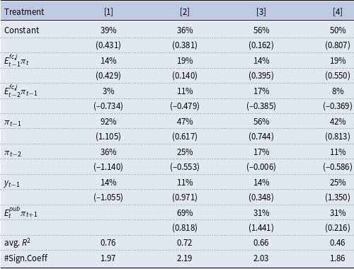
Next, we consider all subjects that were shown a public central bank projection prior to submitting their own forecast. This group consists of all subjects in Treatment 2, 3, and 4, which are displayed in, respectively, Columns [2], [3], and [4] of Table 1. In all three treatments, the percentage of subjects for which the first and second lag of inflation are significant is considerably lower than in Column [1]. The same holds for the absolute value of the median coefficients on these two variables. These results indicate that in the treatments where subjects are presented with a public central bank projection, they rely substantially less on trend following and naive adaptive heuristics.
Turning to the coefficients on the published central bank projections, we find that, in Treatment 2, the central bank projection published by the human central banker has a statistically significant effect on the expectations of 69% of the professional forecaster subjects. In Treatment 3, the percentage of professional forecasters whose forecasts were statistically significantly affected by the published algorithmic projections is lower (31%).Footnote 24 However, considering the magnitude of the estimated coefficients on the published projection, it can be seen in Table 1 that the median of the estimated coefficients is
 $0.8$
in Treatment 2 and
$0.8$
in Treatment 2 and
 $1.4$
in Treatment 3. This implies that subjects put considerable weight on the published projections in both these treatments, and that in Treatment 3 they even (over-)extrapolate the projection in most cases. From this evidence, we conclude that public projections in Treatments 2 and 3 considerably affect subjects’ own forecasts.
$1.4$
in Treatment 3. This implies that subjects put considerable weight on the published projections in both these treatments, and that in Treatment 3 they even (over-)extrapolate the projection in most cases. From this evidence, we conclude that public projections in Treatments 2 and 3 considerably affect subjects’ own forecasts.
For the treatment with random projections (Treatment 4), we also find that the expectations of 31% of subjects are significantly affected by the published projection. However, here the median coefficient of 0.2 implies that, generally, forecasts are only marginally influenced by these rather inaccurate projections.
The bottom row of Table 1 presents the average number of significant regressors used in the expectation formation process in each of the four treatments. Interestingly, this number is around two for all of the four treatments. This leads to the conclusion that subjects rather substitute the public central bank inflation projection for another source of information than complement their information set in the expectation formation process.
5 Macroeconomic Results
Having established that central bank projections influence private-sector expectations, we now turn to the ramifications of this influence for the macroeconomy.
5.1 Coordination of Expectations
Central bank projections are common to all professional forecasters and thereby provide public information. Such public information can act as a focal point, coordinating private-sector expectations (Morris and Shin (Reference Morris and Shin2002)), and thereby giving rise to potential expectations management.
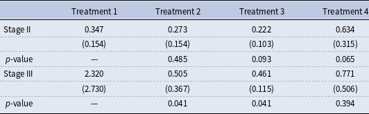
We study the role of central bank projections as coordination device for private-sector expectations by looking at the cross-sectional dispersion of individual expectations to proxy the disagreement among professional forecasters. Following Ehrmann et al. (Reference Ehrmann, Eijffinger and Fratzscher2012) and Hubert (Reference Hubert2014), we measure cross-sectional dispersion by the inter-quartile range of professional forecasts in any given period. Table 2 presents the average median dispersion of professional forecasts per treatment.Footnote 25 The p-values are derived from a series of non-parametric two-sided Wilcoxon rank sum tests. The table shows that although strategic projections (Treatments 2 and 3) reduce the average dispersion roughly by one-third the differences are not statistically significant. Random projections (Treatment 4), by contrast, significantly increase average dispersion, almost doubling it.
Table 2. Average median dispersion of professional forecasts in economies of treatment j (standard deviation in parentheses) for
 $j=1,...,4$
. The p-values result from two-sided Wilcoxon rank sum tests for pairwise comparisons with
$j=1,...,4$
. The p-values result from two-sided Wilcoxon rank sum tests for pairwise comparisons with
 $N=6$
observation of treatment 1 with Treatments 2, 3, and 4.
$N=6$
observation of treatment 1 with Treatments 2, 3, and 4.
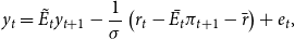
Next, we consider kernel density estimates of per-period dispersion in each economy for each treatment. The more right-skewed a kernel density estimate is, the less dispersed are the elicited individual professional forecasts. The kernel density estimates for each of the four treatments are depicted in Figure 3 in the appendix. To test for significance of statistical differences, a permutation test is applied. Relative to Treatment 1, density estimates are significantly more right-skewed under strategic projections (
 $p<0.05$
) and significantly less right-skewed under random projections (
$p<0.05$
) and significantly less right-skewed under random projections (
 $p<0.01$
). Taken together, these results hint toward an important role of central bank projections for the coordination of private-sector expectations.Footnote 26
$p<0.01$
). Taken together, these results hint toward an important role of central bank projections for the coordination of private-sector expectations.Footnote 26

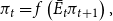
Figure 1. Median responses of inflation (upper panel), the output gap (middle panel), and the interest rate (lower panel) for all four treatments. For each treatment, median responses are generated by taking the median of each inflation, the output gap, and the interest rate from all six economies at each period
 $t=1,...,37$
. Note that for Treatment 1 the median interest rate leaves the zero lower bound despite a deflationary recession. This abnormal artifact is a result from the aggregation procedure (median) as three economies of Treatment 1 remain at the zero lower bound, while three economies leave the zero lower bound (see Figure 5 in the appendix.)
$t=1,...,37$
. Note that for Treatment 1 the median interest rate leaves the zero lower bound despite a deflationary recession. This abnormal artifact is a result from the aggregation procedure (median) as three economies of Treatment 1 remain at the zero lower bound, while three economies leave the zero lower bound (see Figure 5 in the appendix.)
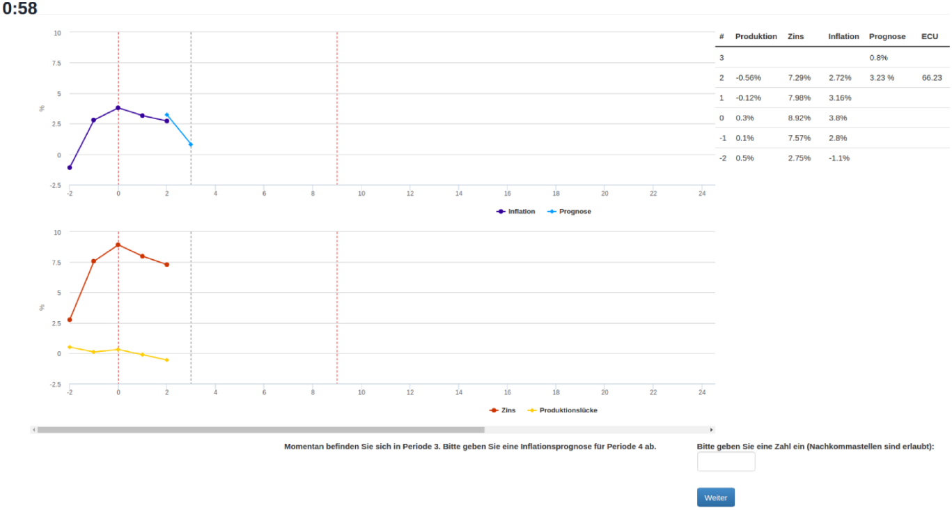
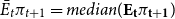
Figure 2. Computer interface as seen by the subjects. The figure shows the graphical and tabular representation of the complete history of the economy as well as the timer and the input box. The exemplary subject is currently in period 3 and she is asked to provide a forecast for period 4.
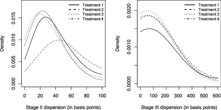
Figure 3. Kernel density estimates of per period dispersion in Stage II (left panel) and Stage III (right panel) per treatment.
To quantify the coordinating effect of public inflation projections, in the spirit of Ehrmann et al. (Reference Ehrmann, Eijffinger and Fratzscher2012) and Hubert (Reference Hubert2014), we estimate a panel model of the form
 \begin{equation} \sigma_{i,t} = constant + \beta_1 PP_{i,t}+ \beta_2 \sigma_{i,t-1} + \beta_3 X_{i,t-1} + \varepsilon_{i,t},\end{equation}
where
 $\sigma_{i,t}$
is the cross-sectional dispersion of the professional forecasters from economy i in period t,
$\sigma_{i,t}$
is the cross-sectional dispersion of the professional forecasters from economy i in period t,
 $PP_{i,t}$
is a dummy variable which takes value 1 when a public inflation projection is present in economy i, and
$PP_{i,t}$
is a dummy variable which takes value 1 when a public inflation projection is present in economy i, and
 $X_{i,t-1}$
is a vector of macroeconomic controls in economy i. The macroeconomic controls
$X_{i,t-1}$
is a vector of macroeconomic controls in economy i. The macroeconomic controls
 $X_{i,t-1}$
comprise the lagged inflation rate, the lagged output gap, and lagged inflation uncertainty defined by
$X_{i,t-1}$
comprise the lagged inflation rate, the lagged output gap, and lagged inflation uncertainty defined by
 $IU_{i,t-1}=|\pi_{i,t-1}-\pi_{i,t-2}|$
, which is the absolute error of a random walk forecast (Ahrens and Hartmann (Reference Ahrens and Hartmann2015)). We expect a positive relationship between lagged inflation uncertainty and the dispersion across individuals. The higher the lagged inflation uncertainty, the harder the prediction of inflation and thereby the greater the dispersion across individuals (Capistrán and Timmermann (Reference Capistrán and Timmermann2009); Dovern and Hartmann (Reference Dovern and Hartmann2017)). Concerning the remaining control variables, first, we expect dispersion to be positively influenced by lagged inflation. Mankiw et al. (Reference Mankiw, Reis and Wolfers2004) show that a higher level of inflation yields more disagreement in inflation expectations. For the lagged output gap, we expect a negative relationship, since Dovern et al. (Reference Dovern, Fritsche and Slacalek2012) and Hubert (Reference Hubert2014) document a higher disagreement in recessions. We estimate equation (13) with random effects and heteroskedasticity-robust standard errors.Footnote 27
$IU_{i,t-1}=|\pi_{i,t-1}-\pi_{i,t-2}|$
, which is the absolute error of a random walk forecast (Ahrens and Hartmann (Reference Ahrens and Hartmann2015)). We expect a positive relationship between lagged inflation uncertainty and the dispersion across individuals. The higher the lagged inflation uncertainty, the harder the prediction of inflation and thereby the greater the dispersion across individuals (Capistrán and Timmermann (Reference Capistrán and Timmermann2009); Dovern and Hartmann (Reference Dovern and Hartmann2017)). Concerning the remaining control variables, first, we expect dispersion to be positively influenced by lagged inflation. Mankiw et al. (Reference Mankiw, Reis and Wolfers2004) show that a higher level of inflation yields more disagreement in inflation expectations. For the lagged output gap, we expect a negative relationship, since Dovern et al. (Reference Dovern, Fritsche and Slacalek2012) and Hubert (Reference Hubert2014) document a higher disagreement in recessions. We estimate equation (13) with random effects and heteroskedasticity-robust standard errors.Footnote 27
The estimation results are summarized in Table 3. Column [1] in Table 3 shows the results when all four treatments are considered. In this case, the publication of inflation projections per se does not affect coordination, that is,
 $PP_{i,t}$
is close to zero and statistically insignificant. A similar result holds for the output gap coefficient. For the complete set of data, cross-sectional dispersion is a persistent phenomenon which is mainly driven by inflation uncertainty. In Columns [2]–[4], we distinguish between strategic and random projections. While Columns [2] and [3] show variants which abstract from random projections (Treatment 4), Column [4] abstracts from strategic projections. Consider Columns [2] and [3] first. Column [2] shows the parameter estimates of (13) using data from Treatments 1 and 2, and Column [3] using data from Treatments 1 and 3. First, the table shows that parameter values generally have the expected sign. Strategic projections unambiguously reduce the dispersion of individual expectations. The reduction is statistically significant. The influence of inflation uncertainty on the dispersion remains statistically significant. The output gap coefficient again is negligible and statistically insignificant. Finally, Column [4] shows the parameter estimates of (13) using data from Treatments 1 and 4 only. Now, the effect of publishing inflation projections is positive and statistically significant. Random projections increase the cross-sectional dispersion by approximately 27%. The results are similar if we consider contemporaneous macroeconomic controls
$PP_{i,t}$
is close to zero and statistically insignificant. A similar result holds for the output gap coefficient. For the complete set of data, cross-sectional dispersion is a persistent phenomenon which is mainly driven by inflation uncertainty. In Columns [2]–[4], we distinguish between strategic and random projections. While Columns [2] and [3] show variants which abstract from random projections (Treatment 4), Column [4] abstracts from strategic projections. Consider Columns [2] and [3] first. Column [2] shows the parameter estimates of (13) using data from Treatments 1 and 2, and Column [3] using data from Treatments 1 and 3. First, the table shows that parameter values generally have the expected sign. Strategic projections unambiguously reduce the dispersion of individual expectations. The reduction is statistically significant. The influence of inflation uncertainty on the dispersion remains statistically significant. The output gap coefficient again is negligible and statistically insignificant. Finally, Column [4] shows the parameter estimates of (13) using data from Treatments 1 and 4 only. Now, the effect of publishing inflation projections is positive and statistically significant. Random projections increase the cross-sectional dispersion by approximately 27%. The results are similar if we consider contemporaneous macroeconomic controls
 $X_{i,t}$
, as applied in the original studies by Ehrmann et al. (Reference Ehrmann, Eijffinger and Fratzscher2012) and Hubert (Reference Hubert2014).
$X_{i,t}$
, as applied in the original studies by Ehrmann et al. (Reference Ehrmann, Eijffinger and Fratzscher2012) and Hubert (Reference Hubert2014).
Table 3. Coordination effect of published projections. The table shows the results from estimating equation (13) with random effects and heteroskedasticity-robust standard errors in parentheses for different subsamples of the experimental data. The respective samples are: [1] T1-T4; [2] T1 vs T2; [3] T1 vs T3; [4] T1 vs T4.
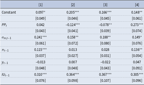
*
 $\ p<0.10$
, **
$\ p<0.10$
, **
 $\ p<0.05$
, ***
$\ p<0.05$
, ***
 $\ p<0.01$
.
$\ p<0.01$
.
Taken together, the above results give rise to the notion that strategic projections act as a coordination device for private-sector inflation expectations, while random projections unleash disturbing forces driving private-sector expectations apart. Therefore, the evidence supports Hypothesis 1.
From a policy maker’s point of view, this coordinating effect can be a useful monetary policy instrument. Eusepi and Preston (Reference Eusepi and Preston2010) point out that in economies with potentially self-fulfilling expectations and learning, expectation may be inconsistent with monetary policy. Therefore, unlike under rational expectations, the Taylor principle alone does not guarantee macroeconomic stability. Central bank projections, by contrast, can generate macroeconomic stabilization through coordination of private-sector expectations on a path consistent with monetary policy. In the following section, we have a closer look at the role of central bank projections for macroeconomic stability.
5.2 Macroeconomic Stability
In this section, we analyze to what extent strategic projections stabilize the economy. To fix ideas, first we juxtapose the median economic dynamics arising from the actual experiment in each of the four treatments and their statistical properties.
Figure 1 shows the median evolution of inflation, the output gap, and the interest rate for all four treatments; Treatment 1 is depicted by the solid lines, Treatment 2 by the dashed lines, Treatment 3 by the dotted lines, and Treatment 4 by the dashed-dotted lines.Footnote 28 The figure shows that all four treatments share a common pattern for the evolution of the macroeconomy over much of the 37 rounds of the experiment. First, there is convergence toward the central bank’s target levels (horizontal gray line). Second, starting in period 29 (the second vertical, gray line), a deep recession takes place which drives the economy toward the zero lower bound. While median economies recover from the recession under strategic projections (Treatments 2–4 in Stage III), the median economy falls into a deflationary spiral in the absence of published projections (Treatment 1).
In Figure 9 in the appendix we plot, for each treatment, the median evolution of inflation against the (median) published projection. Here it can be seen that the small rise in inflation in Treatment 2 in periods 15 and 16 occurs exactly in the periods where the human central bankers publish higher inflation projections. In Treatment 3, no such periods of higher projections arise and inflation dynamics remain close to the target throughout Stage II. Even though inflation dynamics are much more volatile in Treatment 4, no clear relation can be detected between the random published projections in Stage II and the direction of inflation dynamics. This indicates that, at the aggregate level, random projections are largely ignored.
All in all, there are considerable quantitative effects of strategic published projections on macroeconomic stability. In the following, we analyze these effects separately for normal times and for times of severe economic stress.
5.2.1 Macroeconomic stability in normal times
First we analyze the stabilizing role of published central bank inflation projections for the economy in normal times, that is, we focus entirely on Stage II. We evaluate macroeconomic stability by the mean-squared deviations of inflation and the output gap from their respective target values.
 \begin{eqnarray} MSD_ {i,j}^{\pi} &= & \frac{1}{20}\sum_{t=9}^{28}\left(\pi_{t}-\pi^T\right)^2,\end{eqnarray}
 \begin{eqnarray} MSD_ {i,j}^{y} &= & \frac{1}{20}\sum_{t=9}^{28}y_{t}^2.\end{eqnarray}
The lower
 $MSD_ {i,j}^{\pi}$
and
$MSD_ {i,j}^{\pi}$
and
 $MSD_ {i,j}^{y}$
, the more stable the economy. Columns [1]–[4] of Table 4 summarize the treatment-average mean-squared deviation from target for inflation
$MSD_ {i,j}^{y}$
, the more stable the economy. Columns [1]–[4] of Table 4 summarize the treatment-average mean-squared deviation from target for inflation
 $(\bar{MSD}_j^{\pi}=\frac{1}{6}\sum_{i=1}^6 MSD_ {i,j}^{\pi})$
and the output gap
$(\bar{MSD}_j^{\pi}=\frac{1}{6}\sum_{i=1}^6 MSD_ {i,j}^{\pi})$
and the output gap
 $(\bar{MSD}_j^{y}=\frac{1}{6}\sum_{i=1}^6 MSD_ {i,j}^{y})$
. The p-values in Table 4 are derived from a series of non-parametric two-sided Wilcoxon rank sum tests with respect to Treatment 1. Strategic projections (Treatments 2 and 3) reduce
$(\bar{MSD}_j^{y}=\frac{1}{6}\sum_{i=1}^6 MSD_ {i,j}^{y})$
. The p-values in Table 4 are derived from a series of non-parametric two-sided Wilcoxon rank sum tests with respect to Treatment 1. Strategic projections (Treatments 2 and 3) reduce
 $\bar{MSD}_j^{\pi}$
by approximately two-thirds and
$\bar{MSD}_j^{\pi}$
by approximately two-thirds and
 $\bar{MSD}_j^{y}$
by approximately one-third. These differences are statistically significant. Random projections, by contrast, have no statistically significant effect on macroeconomic stability.
$\bar{MSD}_j^{y}$
by approximately one-third. These differences are statistically significant. Random projections, by contrast, have no statistically significant effect on macroeconomic stability.
Table 4. Average mean-squared-deviation of Stage II inflation and the output gap from their respective targets in economies of treatment j (standard deviation in parentheses) for
 $j=1,...,4$
, and of the counterfactual simulations. The p-values in column [2]–[6] result from two-sided Wilcoxon rank sum tests for pairwise comparisons to Treatment 1 with
$j=1,...,4$
, and of the counterfactual simulations. The p-values in column [2]–[6] result from two-sided Wilcoxon rank sum tests for pairwise comparisons to Treatment 1 with
 $N=6$
observation.
$N=6$
observation.

To asses distributional differences in economic stability, we turn to kernel density estimates. Kernel density estimates for
 $MSD_ {i,j}^{\pi}$
and
$MSD_ {i,j}^{\pi}$
and
 $MSD_ {i,j}^{y}$
per treatment are presented in Figure 4 in the appendix. Significance is again tested, by applying a permutation test. Compared to Treatment 1, inflation and output gap are considerably right-skewed (i.e. more stable) in Treatments 2 and 3. These distributional differences are statistically significant for Treatment 2 and 3 inflation (
$MSD_ {i,j}^{y}$
per treatment are presented in Figure 4 in the appendix. Significance is again tested, by applying a permutation test. Compared to Treatment 1, inflation and output gap are considerably right-skewed (i.e. more stable) in Treatments 2 and 3. These distributional differences are statistically significant for Treatment 2 and 3 inflation (
 $p<0.05$
) and for the Treatment 2 output gap (
$p<0.05$
) and for the Treatment 2 output gap (
 $p<0.1$
). Distributional differences between Treatments 1 and 4 are never statistically significant.
$p<0.1$
). Distributional differences between Treatments 1 and 4 are never statistically significant.

Figure 4. Kernel density estimates of economy-average mean-squared deviations of inflation (left panel) and output gap (right panel) from their respective targets per treatment.
The stabilizing role of strategic projections manifests through a much faster convergence of inflation toward its target. In Treatments 2 and 3, inflation reaches the close neighborhood of the inflation target, say an interval of
 $\pm 25$
basis points around the target, on average within 5 periods. In Treatments 1 and 4, time to convergence triples, with a third of the economies not reaching convergence at all during Stage II.
$\pm 25$
basis points around the target, on average within 5 periods. In Treatments 1 and 4, time to convergence triples, with a third of the economies not reaching convergence at all during Stage II.
Since, the mean-squared deviations for inflation and output gap are the main determinants of welfare in the economy, the above analysis implies that strategic projections are an effective instrument to increase welfare through their stabilizing role in the economy.Footnote 29 Random projections, by contrast, remain without statistically significant effects on stabilization. As a result, the above analysis supports Hypothesis 2(a).
5.2.2 Published Central bank projections at the zero lower bound
Next we analyze the impact of strategic inflation projections in times of severe economic stress. To do so, we look at Stage III (periods 29–37) of the experiment. Between periods 29 and 32, a series of four consecutive negative demand shocks of
 $-2.5\%$
annually in periods
$-2.5\%$
annually in periods
 $t=29,...,32$
hits all 24 economies alike. Figure 1 and Figures 5–8 in the appendix show the reaction of the macroeconomies to these shocks. In each case, a deflationary recession takes place, which drives the economy to the zero lower bound on the nominal interest rate. The severity of the economic downturn, however, can be mitigated when the central bank publishes strategic inflation projections. This can be seen from Table 5 where we summarize important key indicators describing the median severity of the economic downturn in each of the four treatments. In the results description below, p-values of the two-sided Wilcoxon rank sum tests are reported only if differences in medians are statistically significant.
$t=29,...,32$
hits all 24 economies alike. Figure 1 and Figures 5–8 in the appendix show the reaction of the macroeconomies to these shocks. In each case, a deflationary recession takes place, which drives the economy to the zero lower bound on the nominal interest rate. The severity of the economic downturn, however, can be mitigated when the central bank publishes strategic inflation projections. This can be seen from Table 5 where we summarize important key indicators describing the median severity of the economic downturn in each of the four treatments. In the results description below, p-values of the two-sided Wilcoxon rank sum tests are reported only if differences in medians are statistically significant.
Table 5. Important key indicators for Stage III. The table shows treatment medians of key indicators describing the severity of the recession and the accompanying liquidity trap in Stage III. The markets where deflationary spirals arise are: T1-4, T1-5, T1-6, T2-5, T4-3.

Figure 5. Resulting aggregate time series for inflation (solid line), the output gap (dashed line), and the interest rate (dotted line) for all six experimental economies of Treatment 1 (control treatment).

Figure 6. Resulting aggregate time series for inflation (solid line), the output gap (dashed line), and the interest rate (dotted line) for all six experimental economies of Treatment 2.

Figure 7. Resulting aggregate time series for inflation (solid line), the output gap (dashed line), and the interest rate (dotted line) for all six experimental economies of Treatment 3.

Figure 8. Resulting aggregate time series for inflation (solid line), the output gap (dashed line), and the interest rate (dotted line) for all six experimental economies of Treatment 4.
Figure 9. Aggregate time series for inflation (solid line) and period t central bank projection for inflation in period
 $t+1$
.
$t+1$
.

Figure 10. Stage III time series for the public central bank inflation projection (solid line), the data-driven forecast (dashed line), the “required for target” (dotted line), and the individual private-sector forecasts (x) for all six experimental economies of Treatment 2. Vertical gray lines denote the four-period fundamental shock sequence.
At this point, it is important to remember that in Treatment 4, random projections are only published in Stage II of the experiment. In Stage III, on the other hand, Treatment 4 features the same algorithmic projections as in Treatment 3. In the current analysis, Treatments 2, 3, and 4 hence all have strategic projections, whereas only Treatment 1 does not.
Table 5 shows that strategic projections on average halve the median time spent at the zero lower bound, from 5 periods in Treatment 1 to less than 2.5 periods on average in Treatments 2–4. Secondly, the length of the recessionFootnote 30 is significantly
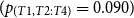 $(p_{(T1,T2:T4)}=0.090)$
reduced from 8 periods in Treatment 1 to less than 4 periods on average in Treatments 2–4. Also, the depth of the recession radically reduces in the presence of strategic projections. We measure the depth of the recession by comparing the latest pre-crisis output gap with the largest negative output gap during the crisis. In Treatment 1, the median depth is a loss in output gap of approximately -240%, whereas this loss is around –4% on average for Treatments 2–4. Prices, in all economies, fall, that is, there is deflation. However, with 6.5 periods on average in Treatments 2–4 median deflation episodes are reduced by 1.5 periods relative to Treatment 1. All qualitative results carry over for pairwise comparisons of Treatment 1 to Treatments 2, 3, and 4.
$(p_{(T1,T2:T4)}=0.090)$
reduced from 8 periods in Treatment 1 to less than 4 periods on average in Treatments 2–4. Also, the depth of the recession radically reduces in the presence of strategic projections. We measure the depth of the recession by comparing the latest pre-crisis output gap with the largest negative output gap during the crisis. In Treatment 1, the median depth is a loss in output gap of approximately -240%, whereas this loss is around –4% on average for Treatments 2–4. Prices, in all economies, fall, that is, there is deflation. However, with 6.5 periods on average in Treatments 2–4 median deflation episodes are reduced by 1.5 periods relative to Treatment 1. All qualitative results carry over for pairwise comparisons of Treatment 1 to Treatments 2, 3, and 4.
Despite binding zero lower bounds and prolonged deflationary episodes, deflationary spirals are rare. However, they occur much more often in the absence of strategic projections than in the presence of strategic projections. In Treatment 1, three out of six economies result in a deflationary spiral after a series of severe fundamental shocks. While deflationary spirals can be avoided successfully in all six economies of Treatment 3, in both Treatments 2 and 4 one out of six economies result in a deflationary spiral. Therefore, published inflation projections significantly
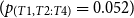 $(p_{(T1,T2:T4)}=0.052)$
reduce the occurrence of deflationary spirals.
$(p_{(T1,T2:T4)}=0.052)$
reduce the occurrence of deflationary spirals.
The stabilizing role of published central bank inflation projections at the zero lower bound is particularly surprising, since at the zero lower bound an overoptimistic (or strategic) inflation projection can by no means be supported with movements of the interest rate. We believe that the evidence presented in this section supports Hypothesis 2(b).
6 Credibility, Strategic-Ness, and Stabilization
In this section, we analyze the relationship between credibility and strategic-ness and its implications for the stabilizing role of published central bank inflation projections. This way, we shed light on the transmission channel through which published inflation projections affect the economy. We argue that the stabilizing effect of published projections functions through the coordination of expectations on the public projection, that is, credibility. A high degree of strategic-ness helps to stabilize the economy only if the projections are credible. In case projections are not credible at all, they are without any effect on the macroeconomy.
As the influences of credibility and strategic-ness are generally interdependent in our experimental setup, we make use of two counterfactual simulations, which allow us to study each channel separately. In these counterfactuals, we assume that central bank projections are fully credible. Under this assumption, all professional forecasters strictly adopt the central bank projection in each period. In the first counterfactual (henceforth: CF1), the central bank publishes the non-strategic data-driven forecast as projection. This counterfactual allows us to isolate the role of credibility. By contrast, in the second counterfactual (henceforth: CF2), the projections are generated by the computer algorithm from Treatment 3. This counterfactual highlights the power of strategic-ness of a credible central bank.
6.1 The Effect of Credibility on Economic Stability
Now, we study in isolation the influence of credibility for the stabilizing role of published central bank inflation projections, that is, we abstract from strategic behavior of the central bank. To do so, we compare CF1 to Treatment 1, that is, Columns [1] and [5] of Table 4. Column [5] of Table 4 shows the average stability measures for inflation and output gap of the six counterfactual economies of CF1, where a fully credible non-strategic projection was available. The average stability measures from CF1 is significantly lower
 $(p<0.05)$
than the stability measures of Treatment 1, where no projection was available.Footnote 31 Thus, coordination of expectations on the path implied by the data-driven forecast increases economic stability, even though these forecasts are non-strategic.
$(p<0.05)$
than the stability measures of Treatment 1, where no projection was available.Footnote 31 Thus, coordination of expectations on the path implied by the data-driven forecast increases economic stability, even though these forecasts are non-strategic.
6.2 The Effect of Strategic-ness on Economic Stability
Next, we study the influence of strategic-ness for the stabilizing role of published central bank inflation projections. We measure the degree of strategic-ness in any period t by the deviation of the published inflation projection from the data-driven forecast, normalized by the necessary deviation from the data-driven forecast to reach the central bank’s target values. This measure is given by
 \begin{equation}SP_t = \frac{E_t^{pub}\pi_{t+1}-E_t^{ddf}\pi_{t+1}}{E_t^{rft}\pi_{t+1}-E_t^{ddf}\pi_{t+1}}.\end{equation}
If
 $SP_t = 0$
, the published projection coincides with the data-driven forecast. This is the case of purely informational behavior. A value
$SP_t = 0$
, the published projection coincides with the data-driven forecast. This is the case of purely informational behavior. A value
 $0 < SP_t < 1$
implies a positive degree of strategic behavior. If
$0 < SP_t < 1$
implies a positive degree of strategic behavior. If
 $SP_t = 1$
, the published projection coincides with the “required for target.” This is the case of perfectly strategic behavior.Footnote 32
$SP_t = 1$
, the published projection coincides with the “required for target.” This is the case of perfectly strategic behavior.Footnote 32
Table 6 summarizes the average session-median strategic-ness for Treatments 2–4 and the two counterfactuals. One-sample Wilcoxon tests show that in Treatments 2 and 3 the average session-median “strategic-ness” measures significantly exceed zero in all of the cases, indicating an overall strategic behavior of the central bank forecaster. Second, the two-sided Wilcoxon signed ranked test finds that the median strategic-ness in Treatment 3 is significantly higher than in Treatment 2 (
 $ p < 0.004 $
). This implies that, although the human central bankers behaved in a strategic manner and actively tried to steer the economy toward the target, they did so to a lesser extent than our computer algorithm.
$ p < 0.004 $
). This implies that, although the human central bankers behaved in a strategic manner and actively tried to steer the economy toward the target, they did so to a lesser extent than our computer algorithm.
Table 6. Average session-median strategic-ness for Treatments 2–4 and the two counterfactuals. Standard deviations in parentheses.
In order to study in isolation (i.e. keeping credibility fixed) the influence of strategic-ness for the stabilizing role of published central bank inflation projections, we compare CF1, where the published projection equals the non-strategic data-driven forecast to CF2, where the published projection follows the strategic algorithm of Treatment 3. In particular, we compare Columns [5] and [6] of Table 4. Column [6] of Table 4 shows the average stability measures for inflation and output gap from the 6 counterfactual economies of CF2. The results show that inflation in CF2 is significantly more stable
 $(p<0.01)$
compared to inflation in CF1. By contrast, for the output gap this difference is only marginally significant
$(p<0.01)$
compared to inflation in CF1. By contrast, for the output gap this difference is only marginally significant
 $(p<0.1)$
. Thus, coordination of expectations on a strategic path implied by the algorithm of Treatment 3, under full credibility, increases further economic stability.
$(p<0.1)$
. Thus, coordination of expectations on a strategic path implied by the algorithm of Treatment 3, under full credibility, increases further economic stability.
CF1 and CF2 also provide insights into the role of strategic-ness at the zero lower bound (i.e. Stage III). In particular, we find that when the central bank publishes the data-driven forecast (CF1) all forced recessions result in a deflationary spiral. By contrast, when the central bank acts strategically (CF2), none of the forced recessions results in a deflationary spiral.
Another particularly illustrative example for the importance of strategic-ness to prevent deflationary spirals can be found when looking at the single economies from Treatment 2. Table 7 summarizes the median strategic-ness measures for the single economies in Stage III. First note the central bank forecaster in economy T2-5. The median “strategic-ness” measure (
 $-0.0050$
) implies that this central bank forecaster does not act strategically at the zero lower bound, but instead resorts fully to the data-driven forecast, which predicts a deflationary spiral. Since projections act as a focal point for private-sector expectations, the economy falls into an expectation-driven deflationary spiral. The central bank forecasters of the other five economies, by contrast, do not publicly predict a deflationary spiral but resort to strategic (in this case overoptimistic) inflation projections. None of their economies experiences a deflationary spiral.Footnote 33
$-0.0050$
) implies that this central bank forecaster does not act strategically at the zero lower bound, but instead resorts fully to the data-driven forecast, which predicts a deflationary spiral. Since projections act as a focal point for private-sector expectations, the economy falls into an expectation-driven deflationary spiral. The central bank forecasters of the other five economies, by contrast, do not publicly predict a deflationary spiral but resort to strategic (in this case overoptimistic) inflation projections. None of their economies experiences a deflationary spiral.Footnote 33
Table 7. Median “strategic-ness” measures (equation (16)) for the human central bank forecasters of Treatment 2.

From the above analysis, we conclude that credibility is the catalyst by which strategic projections translate into the economy, that is, credibility is necessary for strategic projections to work. However, excessive strategic-ness of published projections may hamper credibility through systematic positive or negative forecast errors. The relationship between forecast performance and credibility is subject of the next section.
6.3 The Determinants of Credibility
To analyze the determinants of credibility, we follow Mokhtarzadeh and Petersen (Reference Mokhtarzadeh and Petersen2021) and estimate a series of probit models, where the dependent variable
 $U_t$
is binary taking value 1 if individual professional forecasters utilized the central bank projection and 0 if not. A central bank projection is said to be utilized if an individual professional forecasters forecast is within 5 basis points of the respective central bank projection.Footnote 34 This measure acts as a proxy for our credibility measure from above, as it gives us the increase in the likelihood that a projection is closely followed. In accordance with Mokhtarzadeh and Petersen (Reference Mokhtarzadeh and Petersen2021), our explanatory variable is past forecasting performance of the central bank projections, measured by the absoluteFootnote 35 forecast error from the previous period. As controls, we employ the absolute deviation of previous inflation from the central bank’s inflation target, the professional forecasters previous absolute forecast error, period
$U_t$
is binary taking value 1 if individual professional forecasters utilized the central bank projection and 0 if not. A central bank projection is said to be utilized if an individual professional forecasters forecast is within 5 basis points of the respective central bank projection.Footnote 34 This measure acts as a proxy for our credibility measure from above, as it gives us the increase in the likelihood that a projection is closely followed. In accordance with Mokhtarzadeh and Petersen (Reference Mokhtarzadeh and Petersen2021), our explanatory variable is past forecasting performance of the central bank projections, measured by the absoluteFootnote 35 forecast error from the previous period. As controls, we employ the absolute deviation of previous inflation from the central bank’s inflation target, the professional forecasters previous absolute forecast error, period
 $t-2$
utilization of the central bank projection, and the interaction of the latter two. The interaction term measures the degree to which past shaken confidence in the central bank projection influences the willingness to utilize the central bank projection in the future. Additionally, we control for past aggregate credibility of the central bank projection measured by the period
$t-2$
utilization of the central bank projection, and the interaction of the latter two. The interaction term measures the degree to which past shaken confidence in the central bank projection influences the willingness to utilize the central bank projection in the future. Additionally, we control for past aggregate credibility of the central bank projection measured by the period
 $t-1$
credibility indexFootnote 36, and the subjects cognitive ability measured by the three-item “cognitive reflection test” of Frederick (Reference Frederick2005). The estimation results for Stage II from Treatments 2, 3, and 4 are presented in Table 8.Footnote 37
$t-1$
credibility indexFootnote 36, and the subjects cognitive ability measured by the three-item “cognitive reflection test” of Frederick (Reference Frederick2005). The estimation results for Stage II from Treatments 2, 3, and 4 are presented in Table 8.Footnote 37
Table 8. Determinants of the utilization of central bank projections in Stage II. This table summarizes the results of a series of probit models from Section 6.3, where the dependent variable
 $U_t$
is binary taking value 1 if individual professional forecasters utilized the central bank projection and 0 if not. A central bank projection is said to be utilized if an individual professional forecasters forecast is within 5 basis points of the respective central bank projection. The data used for estimation of the series of probit models stem from Stage II of Treatments 2, 3, and 4. For robustness checks which employ alternative measures of credibility, see Table 14 in the appendix.
$U_t$
is binary taking value 1 if individual professional forecasters utilized the central bank projection and 0 if not. A central bank projection is said to be utilized if an individual professional forecasters forecast is within 5 basis points of the respective central bank projection. The data used for estimation of the series of probit models stem from Stage II of Treatments 2, 3, and 4. For robustness checks which employ alternative measures of credibility, see Table 14 in the appendix.
*
 $\ p<0.10$
, **
$\ p<0.10$
, **
 $\ p<0.05$
, ***
$\ p<0.05$
, ***
 $\ p<0.01$
.
$\ p<0.01$
.
The tables show that central bank projections are more likely to be adopted in the future, if they were accurate in the past, independent of whether the economy functions in normal times or in times of severe economic stress. Consequently, credibility increases in past forecasting performance, confirming Hypothesis 1. Additionally, credibility is a persistent phenomenon. If a professional forecaster adopted the central bank projection in the past or if it was credible in the past, the professional forecasters are more likely to adopt the central bank projection in the future. Even if the adoption of a past projection ex-post turns out to be a disappointment, that is, it resulted in an own large forecast error, the willingness of the professional forecaster to adopt future central bank projections remains unchanged, which can be read from the insignificance of the interaction term in Tables 8 and 13. Subjects seem to pay more attention to the performance of the central bank projections than to reflect on their past behavior and its outcomes. Finally, the probit regressions shows that cognitive ability increases the likelihood to adopt central bank projection.
Finally, we would like to raise a note of caution; although credibility, be it high or low, is a very persistent phenomenon, it can change quickly in response to extreme changes in the economic environment. An illustrative example can be found comparing the severe recessions of Treatments 3 and 4. Whereas the central bank’s average Treatment 3 credibility reduces dramatically when entering the recession in Stage III (from 0.9 in Stage II to 0.5 in Stage III), the average Treatment 4 credibility increases massively (from 0.0 to 0.4) by switching from the random projections in Stage II to the algorithmic projection in Stage III, despite the challenges put forth to the algorithm by the recession.Footnote 38
7 Conclusion
In this paper, we study the stabilizing role of published central bank inflation projections in a standard New Keynesian learning-to-forecast laboratory experiment. Subjects take the role of “professional forecasters” in the private sector who form one-period ahead inflation forecasts. Subjects are provided with a limited understanding of the true data generating process and a public central bank inflation projection. We show that central banks can manage private-sector expectations via the publication of strategic central bank inflation projections and that such expectations management can successfully be applied as an additional monetary policy instrument to stabilize the economy.
In particular, we show that published central bank inflation projections considerably influence the subjects’ expectations formation process. In the absence of published inflation projections, subjects expectation formation process is well characterized as mostly backward-looking with simple trend following. In the presence of published central bank projections, by contrast, the public inflation projection becomes an influential piece of information which starkly diminishes the prevalence of backward-looking expectation formation. Consequently, strategic inflation projections act as a focal point, coordinating expectations by decreasing the dispersion among individual forecasts.
This influence on expectations allows the central bank to stabilize the economy; that is, to bring inflation and output faster and closer toward their respective target values and reduce their volatility over the business cycle. At the zero lower bound, the publication of overly optimistic (i.e. strategic) projections greatly reduces the risk of deflationary spirals. Random inflation projections, by contrast, are generally harmful to the economy as they unleash disturbing forces which give rise to large fluctuations of the economy. Finally, we show that credibility is an important precondition for the stabilizing role of published central bank inflation projections, but that achieving full credibility on the expense of all strategic behavior is not optimal either.
Our results have important implications for central bank practice. We show that published central bank inflation projections are a powerful tool for expectations management and for stabilization policy in normal times and at the zero lower bound. However, while a good track record of accurate forecasts is important for credibility, we find that some strategic-ness in the published projection greatly enhances the stabilizing power of central bank inflation projections. Especially in times of severe economic stress, fully truthful projections may be harmful rather than beneficial.
Acknowledgements
We thank Tiziana Assenza, Frank Heinemann, Cars Hommes, Paul Hubert, Domenico Massaro, Cathrin Mohr, Julián A. Parra-Polanía, and seminar participants of the CREED Seminar at Universiteit van Amsterdam, the DEFAP PhD Seminar at Univeristà Cattolica di Milano, the Macroeconomics Seminar at University of Illinois at Urbana-Champaign, and the Nuremberg Reserach Seminar in Economics at Friedrich-Alexander-Universität Erlangen-Nürnberg for valuable comments. We also thank participants of the 2015 Barcelona LeeX Experimental Economics Summer School in Macroeconomics at Universitat Pompeu Fabra, the 21st WEHIA Annual Workshop in Castellón de la Plana, the EU FP7 project “Integrated Macro-Financial Modeling for Robust Policy Design” (MACFINROBODS), the 8th BES-LAB International Workshop on Theoretical and Experimental Macroeconomics in Stony Brook, and the 9th Conference on Growth and Business Cycles in Theory and Practice in Manchester for fruitful discussions. Finally, we thank two anonymous referees whose comments have greatly improved this paper. All remaining errors are ours.
Financial Support
The authors gratefully acknowledge the financial support of NWO (Dutch Science Foundation) Project No. 40614011 “Monetary and Fiscal Policy under Bounded Rationality and Heterogeneous Expectations” and the DFG (German Research Foundation) through CRC 649 “Economic Risk” and CRC TRR 190 “Rationality and Competition.”
A. Estimation Procedure for Equation (12)
First Formula (12) is estimated with OLS. Then the joint significance of all the coefficients that were found to be individually insignificant in the above regression is tested. If these coefficients are jointly insignificant, all of them are removed. If they are jointly significant, exactly 1 coefficient is removed. The coefficient that is removed is then the individually insignificant coefficient that ranks first in the following order of removal list:
 $\alpha_2, \gamma_1, \beta_2, \delta, \beta_1, \alpha_1, c$
.
$\alpha_2, \gamma_1, \beta_2, \delta, \beta_1, \alpha_1, c$
.
After one or more coefficients are removed, Equation (12) is re-estimated without this (these) coefficient(s). Then the joint significance of the coefficients found to be individually insignificant in the new regression is tested and coefficient(s) are removed according to the same procedure as above. This process is repeated until either a regression is performed where all remaining coefficients are individually significant, or until all coefficients are removed.
B. Proof of “Strategic-ness” Index
Below we prove the following three claims about the “strategic-ness” index,
 $SP_t$
,
of equation (16):
$SP_t$
,
of equation (16):
(a)
 $0<SP_t<1$
implies that the published projection lies in the band between the data-driven forecast and the “required for target” information:
$0<SP_t<1$
implies that the published projection lies in the band between the data-driven forecast and the “required for target” information:
 $E_{t}^{rft}\pi_{t+1}<E_t^{pub}\pi_{t+1}<E_{t}^{ddf}\pi_{t+1}\text{ or } E_t^{ddf}\pi_{t+1}<E_t^{pub}\pi_{t+1}<E_t^{rft}\pi_{t+1}$
(b)
 $SP_t>1$
implies that the published projection lies outside the band of the data-driven forecast and the “required for target” information, on the side of the “required for target”:
$SP_t>1$
implies that the published projection lies outside the band of the data-driven forecast and the “required for target” information, on the side of the “required for target”:
 $E_t^{pub}\pi_{t+1}<E_t^{rft}\pi_{t+1}<E_t^{ddf}\pi_{t+1}\text{ or } E_t^{ddf}\pi_{t+1}<E_t^{rft}\pi_{t+1}<E_t^{pub}\pi_{t+1}$
(c)
 $SP_t<0$
implies that the published projection lies outside the band of the data-driven forecast and the “required for target” information, on the side of the data-driven forecast:
$SP_t<0$
implies that the published projection lies outside the band of the data-driven forecast and the “required for target” information, on the side of the data-driven forecast:
 $E_t^{pub}\pi_{t+1}<E_t^{ddf}\pi_{t+1}<E_t^{rft}\pi_{t+1}\text{ or } E_t^{rft}\pi_{t+1}<E_t^{ddf}\pi_{t+1}<E_t^{pub}\pi_{t+1}$
Proof
: (1) When
 $0<SP_t$
either both numerator and denominator in equation (16) are negative or both are positive:
$0<SP_t$
either both numerator and denominator in equation (16) are negative or both are positive:
(i) Consider that both numerator and denominator are negative. It must be that
 $E_t^{pub}\pi_{t+1}<E_t^{ddf}\pi_{t+1}$
and
$E_t^{pub}\pi_{t+1}<E_t^{ddf}\pi_{t+1}$
and
 $E_t^{rft}\pi_{t+1}<E_t^{ddf}\pi_{t+1}$
. Since the denominator is negative
$E_t^{rft}\pi_{t+1}<E_t^{ddf}\pi_{t+1}$
. Since the denominator is negative
 $SP_t<1$
further implies that
$SP_t<1$
further implies that
 $E_t^{pub}\pi_{t+1}-E_t^{ddf}\pi_{t+1}>E_t^{rft}\pi_{t+1}- E_t^{ddf}\pi_{t+1}$
so that
$E_t^{pub}\pi_{t+1}-E_t^{ddf}\pi_{t+1}>E_t^{rft}\pi_{t+1}- E_t^{ddf}\pi_{t+1}$
so that
 $E_t^{rft}\pi_{t+1}<E_t^{pub}\pi_{t+1}$
and hence
$E_t^{rft}\pi_{t+1}<E_t^{pub}\pi_{t+1}$
and hence
 $E_{t}^{rft}\pi_{t+1}<E_t^{pub}\pi_{t+1}<E_{t}^{ddf}\pi_{t+1}$
.
$E_{t}^{rft}\pi_{t+1}<E_t^{pub}\pi_{t+1}<E_{t}^{ddf}\pi_{t+1}$
.
 $SP_t>1$
, on the other hand, implies that
$SP_t>1$
, on the other hand, implies that
 $E_t^{rft}\pi_{t+1}>E_t^{pub}\pi_{t+1}$
and hence
$E_t^{rft}\pi_{t+1}>E_t^{pub}\pi_{t+1}$
and hence
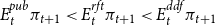 $E_t^{pub}\pi_{t+1}<E_t^{rft}\pi_{t+1}<E_t^{ddf}\pi_{t+1}$
.
$E_t^{pub}\pi_{t+1}<E_t^{rft}\pi_{t+1}<E_t^{ddf}\pi_{t+1}$
.
(ii) Consider that both numerator and denominator are positive.
 $0<SP_t$
implies
$0<SP_t$
implies
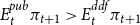 $E_t^{pub}\pi_{t+1}>E_t^{ddf}\pi_{t+1}$
and
$E_t^{pub}\pi_{t+1}>E_t^{ddf}\pi_{t+1}$
and
 $E_t^{rft}\pi_{t+1}>E_t^{ddf}\pi_{t+1}$
.
$E_t^{rft}\pi_{t+1}>E_t^{ddf}\pi_{t+1}$
.
 $SP_t<1$
then implies
$SP_t<1$
then implies
 $E_t^{pub}\pi_{t+1}-E_t^{ddf}\pi_{t+1}<E_t^{rft}\pi_{t+1}- E_t^{ddf}\pi_{t+1}$
so that
$E_t^{pub}\pi_{t+1}-E_t^{ddf}\pi_{t+1}<E_t^{rft}\pi_{t+1}- E_t^{ddf}\pi_{t+1}$
so that
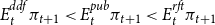 $E_t^{ddf}\pi_{t+1}<E_t^{pub}\pi_{t+1}<E_t^{rft}\pi_{t+1}$
, while
$E_t^{ddf}\pi_{t+1}<E_t^{pub}\pi_{t+1}<E_t^{rft}\pi_{t+1}$
, while
 $SP_t>1$
implies
$SP_t>1$
implies
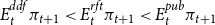 $E_t^{ddf}\pi_{t+1}<E_t^{rft}\pi_{t+1}<E_t^{pub}\pi_{t+1}$
. This completes the proof of (a) and (b).
$E_t^{ddf}\pi_{t+1}<E_t^{rft}\pi_{t+1}<E_t^{pub}\pi_{t+1}$
. This completes the proof of (a) and (b).
(2) When
 $SP_t<0$
, either the numerator of equation (16) is negative while the denominator is positive, or the numerator is positive while the denominator is negative: In the first case, it must hold that
$SP_t<0$
, either the numerator of equation (16) is negative while the denominator is positive, or the numerator is positive while the denominator is negative: In the first case, it must hold that
 $E_t^{pub}\pi_{t+1}<E_t^{ddf}\pi_{t+1}$
while
$E_t^{pub}\pi_{t+1}<E_t^{ddf}\pi_{t+1}$
while
 $E_t^{rft}\pi_{t+1}>E_t^{ddf}\pi_{t+1}$
. In the second case, it must hold that
$E_t^{rft}\pi_{t+1}>E_t^{ddf}\pi_{t+1}$
. In the second case, it must hold that
 $E_t^{pub}\pi_{t+1}>E_t^{ddf}\pi_{t+1}$
while
$E_t^{pub}\pi_{t+1}>E_t^{ddf}\pi_{t+1}$
while
 $E_t^{rft}\pi_{t+1}<E_t^{ddf}\pi_{t+1}$
. This proves (c).
$E_t^{rft}\pi_{t+1}<E_t^{ddf}\pi_{t+1}$
. This proves (c).
C. Additional Tables and Figures
Table 9. Descriptive Statistics of Treatment 1 (Control). The table summarizes mean, median, and variance in each of the three stages for each of the six economies of Treatment 1 as well as their corresponding averages over all six economies of Treatment 1.
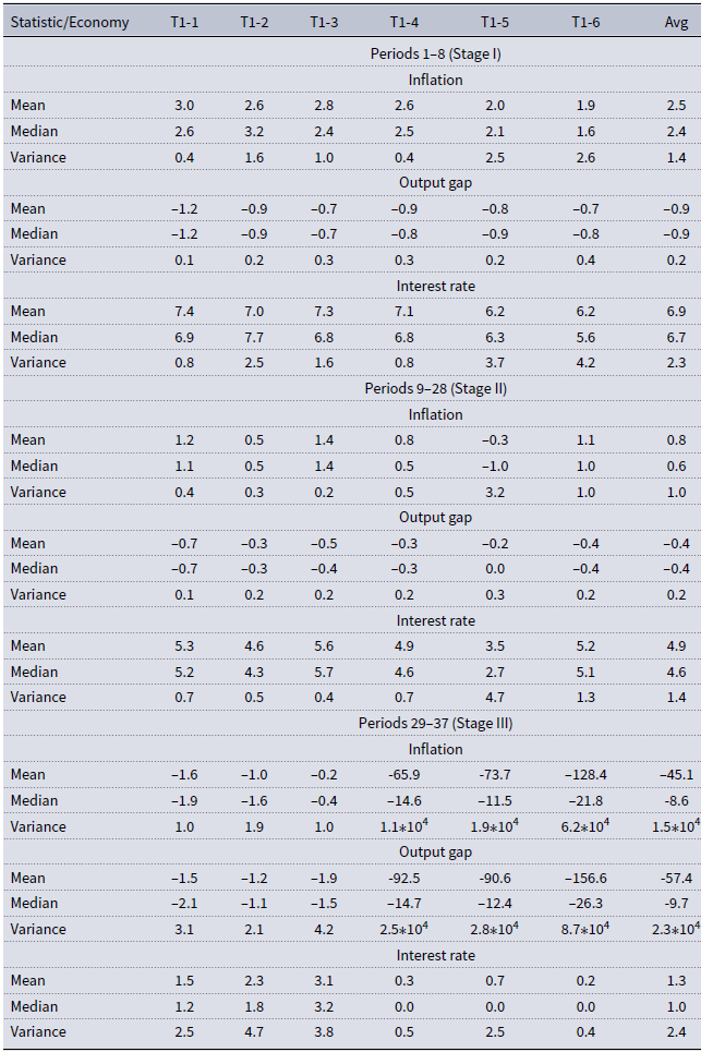
Table 10. Descriptive Statistics of Treatment 2. The table summarizes mean, median, and variance in each of the three stages for each of the six economies of Treatment 2 as well as their corresponding averages over all six economies of Treatment 2.

Table 11. Descriptive Statistics of Treatment 3. The table summarizes mean, median, and variance in each of the three stages for each of the six economies of Treatment 3 as well as their corresponding averages over all six economies of Treatment 3.
Table 12. Descriptive statistics of Treatment 4. The table summarizes mean, median, and variance in each of the three stages for each of the six economies of Treatment 4 as well as their corresponding averages over all six economies of Treatment 4.

Table 13. Determinants of the utilization of central bank projections in Stage III. This table summarizes the results of a series of probit models from Section 6.3, where the dependent variable
 $U_t$
is binary taking value 1 if individual professional forecasters utilized the central bank projection and 0 if not. A central bank projection is said to be utilized if an individual professional forecasters forecast is within 5 basis points of the respective central bank projection. The data used for estimation of the series of probit models stem from Stage II of Treatments 2, 3, and 4.
$U_t$
is binary taking value 1 if individual professional forecasters utilized the central bank projection and 0 if not. A central bank projection is said to be utilized if an individual professional forecasters forecast is within 5 basis points of the respective central bank projection. The data used for estimation of the series of probit models stem from Stage II of Treatments 2, 3, and 4.
*
 $\ p<0.10$
, **
$\ p<0.10$
, **
 $\ p<0.05$
, ***
$\ p<0.05$
, ***
 $\ p<0.01$
.
$\ p<0.01$
.
Table 14. The table presents several robustness checks with respect to the credibility measures for a series of probit models from Section 6.3 (i.e. Table 8). The dependent variable
 $U_t$
is binary, taking value 1 if individual professional forecasters utilized the central bank projection and 0 if not. A central bank projection is said to be utilized if an individual professional forecasters forecast is within 5 basis points of the respective central bank projection. The data used for estimation of the series of probit models stem from Stage II of Treatments 2, 3, and 4. The alternative credibility measures include: [1] a normalized credibility index analogous to equation (10) but with the squared deviation divided by the average stability of the economy given by equation (14); [2] a normalized credibility index similar to the previous case but with a scaling coefficient of
$U_t$
is binary, taking value 1 if individual professional forecasters utilized the central bank projection and 0 if not. A central bank projection is said to be utilized if an individual professional forecasters forecast is within 5 basis points of the respective central bank projection. The data used for estimation of the series of probit models stem from Stage II of Treatments 2, 3, and 4. The alternative credibility measures include: [1] a normalized credibility index analogous to equation (10) but with the squared deviation divided by the average stability of the economy given by equation (14); [2] a normalized credibility index similar to the previous case but with a scaling coefficient of
 $1.4$
instead of 3 to make the normalized measure comparable in terms of average magnitude to the non-normalized measure; [3] an average of two surveyed credibility measures from periods 18 and 28; [4]+[5] a surveyed credibility measures from period 9 to elicit a prior belief about central bank credibility credibility. For more detailed information about the surveyed measures, refer to footnote 8. Note that the results of models [4] and [5] present a particularly interesting insight, since it implies that it is not credibility per se that increases the likelihood of adoption of the central bank projection, but the experience with the projections as implied by the previous results.
$1.4$
instead of 3 to make the normalized measure comparable in terms of average magnitude to the non-normalized measure; [3] an average of two surveyed credibility measures from periods 18 and 28; [4]+[5] a surveyed credibility measures from period 9 to elicit a prior belief about central bank credibility credibility. For more detailed information about the surveyed measures, refer to footnote 8. Note that the results of models [4] and [5] present a particularly interesting insight, since it implies that it is not credibility per se that increases the likelihood of adoption of the central bank projection, but the experience with the projections as implied by the previous results.
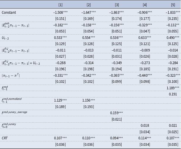
*
 $\ p<0.10$
, **
$\ p<0.10$
, **
 $\ p<0.05$
, ***
$\ p<0.05$
, ***
 $\ p<0.01$
.
$\ p<0.01$
.


 Open access