


1 Introduction
Symmetry transformations – changes in the dependent and independent variables of a physical model that leave the model equations unchanged – are revealing and useful throughout theoretical physics. The most general scheme for uncovering point symmetries of a system of equations is Lie-group analysis (see, e.g. Olver Reference Olver1993; Cantwell Reference Cantwell2002). This scheme has been used extensively in plasma physics, including studies of the Vlasov–Maxwell model for an unmagnetized plasma (see Roberts Reference Roberts1985; Kovalev, Krivenko & Pustovalev Reference Kovalev, Krivenko and Pustovalev1996), charged particle motion in electromagnetic fields (Qin & Davidson Reference Qin and Davidson2006) and the Grad–Shafranov equation (White & Hazeltine Reference White and Hazeltine2009). A special case of Lie symmetry, scaling symmetry, was fruitfully employed by Connor & Taylor (Reference Connor and Taylor1977). In this work we apply the Lie procedure to a particular nonlinear gyrokinetic fluid model used in magnetized plasma turbulence and magnetic reconnection studies.
The symmetries of any physical model have intrinsic interest, especially because one often uncovers unexpected symmetries – beyond the usual rotations, translations and so on which are obvious from physical considerations. Knowledge of the symmetries can simplify numerical calculations, while providing useful tests on their accuracy. When a variational principle is available, the symmetries can be used to identify dynamical constants. They can also be used to generate new solutions from old ones – in particular, physically interesting solutions can be constructed by applying the group operator to a trivial, less interesting solution. Finally, in many cases symmetries can be used to reduce the order of a differential equation system, in some cases leading to exact solutions.
1.1 Fluid-gyrokinetic model
A magnetized plasma is one in which the ion gyroradius, $\unicode[STIX]{x1D70C}_{i}$
, is small compared to all equilibrium gradient scale lengths. However, scale lengths of perturbed quantities in a magnetized plasma, measured by the perpendicular wavelength
$\unicode[STIX]{x1D70C}_{i}$
, is small compared to all equilibrium gradient scale lengths. However, scale lengths of perturbed quantities in a magnetized plasma, measured by the perpendicular wavelength $k_{\bot }^{-1}$
, can break this ordering:
$k_{\bot }^{-1}$
, can break this ordering: $k_{\bot }\unicode[STIX]{x1D70C}_{i}\sim 1$
. Theories allowing for such finite-Larmor-radius (FLR) effects increasingly dominate plasma physics research, entering both kinetic and fluid models of plasma dynamics.
$k_{\bot }\unicode[STIX]{x1D70C}_{i}\sim 1$
. Theories allowing for such finite-Larmor-radius (FLR) effects increasingly dominate plasma physics research, entering both kinetic and fluid models of plasma dynamics.
There are two ways in which conventional fluid equations fall short in their description of magnetized plasma dynamics. First, they represent FLR effects crudely, retaining at most terms of second order in $k_{\bot }\unicode[STIX]{x1D70C}_{i}$
. Second, they entirely omit Landau resonances, which, in the magnetized context, enter through wave–particle interactions parallel to the field – effects conventionally treated by the drift-kinetic equation. Gyrokinetics (Rutherford & Frieman Reference Rutherford and Frieman1968; Taylor & Hastie Reference Taylor and Hastie1968; Catto Reference Catto1978; Catto, Tang & Baldwin Reference Catto, Tang and Baldwin1981; Frieman & Chen Reference Frieman and Chen1982; Dubin et al.
Reference Dubin, Krommes, Oberman and Lee1983; Lee Reference Lee1983, Reference Lee1987; Hahm, Lee & Brizard Reference Hahm, Lee and Brizard1988; Brizard Reference Brizard1992) addresses both shortcomings, providing in particular a full FLR treatment of the perturbed fields, with however the expense and complexity of computation (analytical and numerical) in five dimensions of phase space. Gyrofluid models reduce this overhead by restricting the FLR physics to coordinate space (see, for example, Hammett & Perkins Reference Hammett and Perkins1990; Hammett, Dorland & Perkins Reference Hammett, Dorland and Perkins1992; Dorland & Hammett Reference Dorland and Hammett1993; Hammett et al.
Reference Hammett, Beer, Dorland, Cowley and Smith1993; Beer & Hammett Reference Beer and Hammett1996; Snyder & Hammett Reference Snyder and Hammett2001; Waelbroeck, Hazeltine & Morrison Reference Waelbroeck, Hazeltine and Morrison2009; Bian & Kontar Reference Bian and Kontar2010). However, the validity of the approximations made in their derivation can be hard to ascertain, especially in nonlinear contexts (Dimits et al.
Reference Dimits, Bateman, Beer, Cohen, Dorland, Hammett, Kim, Kinsey, Kotschenreuther and Kritz2000).
$k_{\bot }\unicode[STIX]{x1D70C}_{i}$
. Second, they entirely omit Landau resonances, which, in the magnetized context, enter through wave–particle interactions parallel to the field – effects conventionally treated by the drift-kinetic equation. Gyrokinetics (Rutherford & Frieman Reference Rutherford and Frieman1968; Taylor & Hastie Reference Taylor and Hastie1968; Catto Reference Catto1978; Catto, Tang & Baldwin Reference Catto, Tang and Baldwin1981; Frieman & Chen Reference Frieman and Chen1982; Dubin et al.
Reference Dubin, Krommes, Oberman and Lee1983; Lee Reference Lee1983, Reference Lee1987; Hahm, Lee & Brizard Reference Hahm, Lee and Brizard1988; Brizard Reference Brizard1992) addresses both shortcomings, providing in particular a full FLR treatment of the perturbed fields, with however the expense and complexity of computation (analytical and numerical) in five dimensions of phase space. Gyrofluid models reduce this overhead by restricting the FLR physics to coordinate space (see, for example, Hammett & Perkins Reference Hammett and Perkins1990; Hammett, Dorland & Perkins Reference Hammett, Dorland and Perkins1992; Dorland & Hammett Reference Dorland and Hammett1993; Hammett et al.
Reference Hammett, Beer, Dorland, Cowley and Smith1993; Beer & Hammett Reference Beer and Hammett1996; Snyder & Hammett Reference Snyder and Hammett2001; Waelbroeck, Hazeltine & Morrison Reference Waelbroeck, Hazeltine and Morrison2009; Bian & Kontar Reference Bian and Kontar2010). However, the validity of the approximations made in their derivation can be hard to ascertain, especially in nonlinear contexts (Dimits et al.
Reference Dimits, Bateman, Beer, Cohen, Dorland, Hammett, Kim, Kinsey, Kotschenreuther and Kritz2000).
An alternative and conceptually straightforward approach combines a fluid treatment of the perpendicular physics with a drift-kinetic description, including resonances and collisions, of the parallel dynamics (Ramos Reference Ramos2010, Reference Ramos2011). Such a hybrid approach was proposed and applied as early as 1956 (Chew, Goldberger & Low Reference Chew, Goldberger and Low1956; Grad Reference Grad1956; Kruskal & Oberman Reference Kruskal and Oberman1958; Rosenbluth & Rostoker Reference Rosenbluth and Rostoker1959). Called ‘kinetic magnetohydrodynamics (MHD)’, the early approach neglected most FLR effects, combining MHD with the drift-kinetic equation. However in other respects it resembles the gyrokinetic fluid hybrid considered here.
We study a particular representative of the fluid-kinetic approach: the reduced gyrokinetic model derived in Zocco & Schekochihin (Reference Zocco and Schekochihin2011), referred to below as ZS. The model uses five fields – five functions of five independent variables (including time). To make this work self-contained, and establish notation, we start by reviewing the physical assumptions built into the ZS model in § 2.1, and then express the model equations in normalized variables in § 2.2. The remainder of the paper exclusively uses normalized variables, so the reader who is already familiar with the model can skip § 2.1. The symmetries obtained from our analysis are shown in § 3. Section 4 presents new exact solutions of the reduced MHD (RMHD) equations – a limit of the ZS model – obtained using symmetry transformations. In § 5 we display the Lie-group generator and present the procedure used to derive the symmetries for the (integro-differential) ZS model. We do not attempt any full exegesis of the Lie procedure; readers unfamiliar with it may consult such texts as Olver (Reference Olver1993) or Cantwell (Reference Cantwell2002). Our conclusions are summarized and discussed in § 6.
2 Model equations
2.1 Introduction
The detailed derivation of the ZS model from the gyrokinetic equations is given in Zocco & Schekochihin (Reference Zocco and Schekochihin2011). Here, we briefly survey the physical assumptions, summarize the resulting equations and indicate the physical meaning of each of the fields.
The plasma, composed of electrons with charge $-e$
and ions with charge
$-e$
and ions with charge $Ze$
, is assumed to have a uniform background magnetic field
$Ze$
, is assumed to have a uniform background magnetic field $B_{0}\,\hat{\boldsymbol{z}}$
, and the equilibrium electrons and ions are Maxwellian:
$B_{0}\,\hat{\boldsymbol{z}}$
, and the equilibrium electrons and ions are Maxwellian:
 $$\begin{eqnarray}\displaystyle & \displaystyle F_{0s}={\displaystyle \frac{n_{0s}}{(2\unicode[STIX]{x03C0})^{3/2}v_{Ts}^{3}}}\text{exp}\left(-{\displaystyle \frac{v^{2}}{2v_{Ts}^{2}}}\right), & \displaystyle\end{eqnarray}$$
with $v_{Ts}=(T_{0s}/m_{s})^{1/2}$
. Here we deviate from the convention of Zocco & Schekochihin (Reference Zocco and Schekochihin2011), where the Maxwellian is characterized by its most probable speed
$v_{Ts}=(T_{0s}/m_{s})^{1/2}$
. Here we deviate from the convention of Zocco & Schekochihin (Reference Zocco and Schekochihin2011), where the Maxwellian is characterized by its most probable speed $v_{\text{th},s}=\sqrt{2}v_{Ts}$
. This translates to a slightly different definition of the Larmor radius, which for us is defined by
$v_{\text{th},s}=\sqrt{2}v_{Ts}$
. This translates to a slightly different definition of the Larmor radius, which for us is defined by $\unicode[STIX]{x1D70C}_{s}=v_{Ts}/|\unicode[STIX]{x1D6FA}_{s}|$
, with
$\unicode[STIX]{x1D70C}_{s}=v_{Ts}/|\unicode[STIX]{x1D6FA}_{s}|$
, with $\unicode[STIX]{x1D6FA}_{s}=q_{s}B_{0}/(m_{s}c)$
. This modification eliminates many factors of
$\unicode[STIX]{x1D6FA}_{s}=q_{s}B_{0}/(m_{s}c)$
. This modification eliminates many factors of $\sqrt{2}$
in the final equations.
$\sqrt{2}$
in the final equations.
In accordance with the standard $\unicode[STIX]{x1D6FF}f$
gyrokinetic ansatz, each field is split into its background value plus a small perturbation, with
$\unicode[STIX]{x1D6FF}f$
gyrokinetic ansatz, each field is split into its background value plus a small perturbation, with $\unicode[STIX]{x1D6FF}f_{s}/F_{0s}\sim \unicode[STIX]{x1D6FF}\boldsymbol{B}/\boldsymbol{B}_{0}\sim \boldsymbol{k}_{\Vert }/k_{\bot }\sim \unicode[STIX]{x1D714}/\unicode[STIX]{x1D6FA}_{s}\sim \unicode[STIX]{x1D716}\ll 1$
. Additionally,
$\unicode[STIX]{x1D6FF}f_{s}/F_{0s}\sim \unicode[STIX]{x1D6FF}\boldsymbol{B}/\boldsymbol{B}_{0}\sim \boldsymbol{k}_{\Vert }/k_{\bot }\sim \unicode[STIX]{x1D714}/\unicode[STIX]{x1D6FA}_{s}\sim \unicode[STIX]{x1D716}\ll 1$
. Additionally, $\unicode[STIX]{x1D6FD}_{s}=8\unicode[STIX]{x03C0}n_{0s}T_{0s}/B_{0}^{2}$
is ordered via
$\unicode[STIX]{x1D6FD}_{s}=8\unicode[STIX]{x03C0}n_{0s}T_{0s}/B_{0}^{2}$
is ordered via $\unicode[STIX]{x1D6FD}_{s}\sim Zm_{e}/m_{i}$
, with the mass ratio being treated as a second formal small parameter.
$\unicode[STIX]{x1D6FD}_{s}\sim Zm_{e}/m_{i}$
, with the mass ratio being treated as a second formal small parameter.
2.1.1 Electrostatic ions
After ordering out electromagnetic effects and parallel streaming in the ion gyrokinetic equation, the leading-order ion distribution function is given by
 $$\begin{eqnarray}\displaystyle & \displaystyle \unicode[STIX]{x1D6FF}f_{i}={\displaystyle \frac{ZeF_{0i}}{\unicode[STIX]{x1D70F}T_{0e}}}(\langle \unicode[STIX]{x1D711}\rangle _{\boldsymbol{R}_{i}}-\unicode[STIX]{x1D711}), & \displaystyle\end{eqnarray}$$
where $\boldsymbol{R}_{i}(\boldsymbol{r},\boldsymbol{v})=\boldsymbol{r}-\unicode[STIX]{x1D6FA}_{i}^{-1}\boldsymbol{v}\times \hat{\boldsymbol{z}}$
,
$\boldsymbol{R}_{i}(\boldsymbol{r},\boldsymbol{v})=\boldsymbol{r}-\unicode[STIX]{x1D6FA}_{i}^{-1}\boldsymbol{v}\times \hat{\boldsymbol{z}}$
, $\unicode[STIX]{x1D6FA}_{i}=Ze\boldsymbol{B}_{0}/(m_{i}c)$
,
$\unicode[STIX]{x1D6FA}_{i}=Ze\boldsymbol{B}_{0}/(m_{i}c)$
, $\unicode[STIX]{x1D70F}=T_{0i}/T_{0e}$
and
$\unicode[STIX]{x1D70F}=T_{0i}/T_{0e}$
and $\langle \cdots \,\rangle _{\boldsymbol{R}_{i}}$
denotes the gyroaverage at fixed
$\langle \cdots \,\rangle _{\boldsymbol{R}_{i}}$
denotes the gyroaverage at fixed $\boldsymbol{R}_{i}$
.
$\boldsymbol{R}_{i}$
.
It follows that the ion density perturbation $\unicode[STIX]{x1D6FF}n_{i}$
and mean parallel flow
$\unicode[STIX]{x1D6FF}n_{i}$
and mean parallel flow $u_{\Vert ,i}$
are given by
$u_{\Vert ,i}$
are given by
 $$\begin{eqnarray}\displaystyle & \displaystyle {\displaystyle \frac{\unicode[STIX]{x1D6FF}n_{i}}{n_{0i}}}=-{\displaystyle \frac{Z}{\unicode[STIX]{x1D70F}}}(1-\hat{\unicode[STIX]{x1D6E4}}_{0}){\displaystyle \frac{e\unicode[STIX]{x1D711}}{T_{0e}}}, & \displaystyle\end{eqnarray}$$
 $$\begin{eqnarray}\displaystyle & \displaystyle u_{\Vert ,i}=0, & \displaystyle\end{eqnarray}$$
where $\hat{\unicode[STIX]{x1D6E4}}_{0}$
is an ion gyroaveraging operator:
$\hat{\unicode[STIX]{x1D6E4}}_{0}$
is an ion gyroaveraging operator:
 $$\begin{eqnarray}\displaystyle & \displaystyle \hat{\unicode[STIX]{x1D6E4}}_{0}[\cdots \,]\equiv {\displaystyle \frac{1}{n_{0i}}}\int \text{d}^{3}\boldsymbol{v}\langle \langle \cdots \rangle _{\boldsymbol{R}_{i}}\rangle _{\boldsymbol{r}}F_{0i}(\boldsymbol{v}). & \displaystyle\end{eqnarray}$$
In Fourier space, $\unicode[STIX]{x1D6E4}_{0}$
has the closed-form expression
$\unicode[STIX]{x1D6E4}_{0}$
has the closed-form expression
 $$\begin{eqnarray}\displaystyle & \displaystyle \unicode[STIX]{x1D6E4}_{0}=\text{I}_{0}(\unicode[STIX]{x1D6FC}_{i})\text{e}^{-\unicode[STIX]{x1D6FC}_{i}}, & \displaystyle\end{eqnarray}$$
where $\text{I}_{0}$
is the zeroth-order modified Bessel function and
$\text{I}_{0}$
is the zeroth-order modified Bessel function and $\unicode[STIX]{x1D6FC}_{i}=k_{\bot }^{2}\unicode[STIX]{x1D70C}_{i}^{2}$
.
$\unicode[STIX]{x1D6FC}_{i}=k_{\bot }^{2}\unicode[STIX]{x1D70C}_{i}^{2}$
.
2.1.2 Quasineutrality and Ampère’s law
Since $u_{\Vert ,i}=0$
, we have
$u_{\Vert ,i}=0$
, we have $J_{\Vert }=-en_{0e}u_{\Vert e}$
, and thus the parallel component of Ampère’s law becomes
$J_{\Vert }=-en_{0e}u_{\Vert e}$
, and thus the parallel component of Ampère’s law becomes
 $$\begin{eqnarray}\displaystyle & \displaystyle u_{\Vert ,e}={\displaystyle \frac{e}{m_{e}c}}d_{e}^{2}\unicode[STIX]{x1D6FB}_{\bot }^{2}A_{\Vert }, & \displaystyle\end{eqnarray}$$
where $d_{e}=c/\unicode[STIX]{x1D714}_{pe}$
and
$d_{e}=c/\unicode[STIX]{x1D714}_{pe}$
and $\unicode[STIX]{x1D714}_{pe}=(4\unicode[STIX]{x03C0}n_{e}e^{2}/m_{e})^{1/2}$
.
$\unicode[STIX]{x1D714}_{pe}=(4\unicode[STIX]{x03C0}n_{e}e^{2}/m_{e})^{1/2}$
.
According to equation (2.3), quasineutrality is expressed by
 $$\begin{eqnarray}\displaystyle & \displaystyle {\displaystyle \frac{\unicode[STIX]{x1D6FF}n_{e}}{n_{0e}}}=-{\displaystyle \frac{Z}{\unicode[STIX]{x1D70F}}}(1-\hat{\unicode[STIX]{x1D6E4}}_{0}){\displaystyle \frac{e\unicode[STIX]{x1D711}}{T_{0e}}}. & \displaystyle\end{eqnarray}$$
2.1.3 Drift-kinetic electrons
The electrons are described by a distribution function $g_{e}$
from which the density and parallel flow terms have been extracted:
$g_{e}$
from which the density and parallel flow terms have been extracted:
 $$\begin{eqnarray}\displaystyle & \displaystyle g_{e}=\unicode[STIX]{x1D6FF}f_{e}-\left({\displaystyle \frac{\unicode[STIX]{x1D6FF}n_{e}}{n_{0e}}}-v_{\Vert }{\displaystyle \frac{u_{\Vert ,e}}{v_{Te}^{2}}}\right)F_{0e}. & \displaystyle\end{eqnarray}$$
The electron dynamics is described by fluid equations for the explicit moments, together with a simplified drift-kinetic equation:
 $$\begin{eqnarray}\displaystyle & \displaystyle {\displaystyle \frac{\text{d}}{\text{d}t}}{\displaystyle \frac{\unicode[STIX]{x1D6FF}n_{e}}{n_{0e}}}=-\hat{\boldsymbol{b}}\boldsymbol{\cdot }\unicode[STIX]{x1D735}u_{\Vert e}, & \displaystyle\end{eqnarray}$$
 $$\begin{eqnarray}\displaystyle & \displaystyle m_{e}{\displaystyle \frac{\text{d}}{\text{d}t}}u_{\Vert e}=-\unicode[STIX]{x1D708}_{ei}m_{e}u_{\Vert e}+e\left({\displaystyle \frac{\unicode[STIX]{x2202}\unicode[STIX]{x1D711}}{\unicode[STIX]{x2202}z}}+{\displaystyle \frac{1}{c}}{\displaystyle \frac{\text{d}}{\text{d}t}}A_{\Vert }\right)-T_{0e}\hat{\boldsymbol{b}}\boldsymbol{\cdot }\unicode[STIX]{x1D735}\left({\displaystyle \frac{\unicode[STIX]{x1D6FF}n_{e}}{n_{0e}}}+{\displaystyle \frac{\unicode[STIX]{x1D6FF}T_{\Vert ,e}}{T_{0e}}}\right)\!, & \displaystyle\end{eqnarray}$$
where
 $$\begin{eqnarray}\displaystyle & \displaystyle {\displaystyle \frac{\unicode[STIX]{x1D6FF}T_{\Vert ,e}}{T_{0e}}}={\displaystyle \frac{1}{n_{0e}}}\int \text{d}^{3}\boldsymbol{v}{\displaystyle \frac{v_{\Vert }^{2}}{v_{Te}^{2}}}g_{e}, & \displaystyle\end{eqnarray}$$
is the electron temperature perturbation. We have also introduced the convective time derivative
 $$\begin{eqnarray}\displaystyle & \displaystyle {\displaystyle \frac{\text{d}f}{\text{d}t}}\equiv {\displaystyle \frac{\unicode[STIX]{x2202}f}{\unicode[STIX]{x2202}t}}+{\displaystyle \frac{c}{B_{0}}}\{\unicode[STIX]{x1D711},f\}, & \displaystyle\end{eqnarray}$$
with the Poisson bracket defined by
 $$\begin{eqnarray}\displaystyle & \displaystyle \{\,f,g\}\equiv {\displaystyle \frac{\unicode[STIX]{x2202}f}{\unicode[STIX]{x2202}x}}{\displaystyle \frac{\unicode[STIX]{x2202}g}{\unicode[STIX]{x2202}y}}-{\displaystyle \frac{\unicode[STIX]{x2202}f}{\unicode[STIX]{x2202}y}}{\displaystyle \frac{\unicode[STIX]{x2202}g}{\unicode[STIX]{x2202}x}}, & \displaystyle\end{eqnarray}$$
and the parallel gradient operator
 $$\begin{eqnarray}\displaystyle & \displaystyle \hat{\boldsymbol{b}}\boldsymbol{\cdot }\unicode[STIX]{x1D735}f\equiv {\displaystyle \frac{\unicode[STIX]{x2202}f}{\unicode[STIX]{x2202}z}}-{\displaystyle \frac{1}{B_{0}}}\{A_{\Vert },f\}. & \displaystyle\end{eqnarray}$$
The remaining distribution function $g_{e}$
is determined by a simplified drift-kinetic equation:
$g_{e}$
is determined by a simplified drift-kinetic equation:
 $$\begin{eqnarray}\displaystyle & \displaystyle {\displaystyle \frac{\text{d}g_{e}}{\text{d}t}}+v_{\Vert }\hat{\boldsymbol{b}}\boldsymbol{\cdot }\unicode[STIX]{x1D735}\left(g_{e}-{\displaystyle \frac{\unicode[STIX]{x1D6FF}T_{\Vert ,e}}{T_{0e}}}F_{0e}\right)-C[g_{e}]=\left(1-{\displaystyle \frac{v_{\Vert }^{2}}{v_{Te}^{2}}}\right)F_{0e}\hat{\boldsymbol{b}}\boldsymbol{\cdot }\unicode[STIX]{x1D735}u_{\Vert ,e}, & \displaystyle\end{eqnarray}$$
in which electron FLR terms, as well as curvature drifts, are ordered out by the strong guide field. Finally,
 $$\begin{eqnarray}\displaystyle & \displaystyle C[g_{e}]=\unicode[STIX]{x1D708}_{ei}\Bigg[v_{Te}^{2}{\displaystyle \frac{\unicode[STIX]{x2202}}{\unicode[STIX]{x2202}v_{\Vert }}}\left({\displaystyle \frac{\unicode[STIX]{x2202}}{\unicode[STIX]{x2202}v_{\Vert }}}+{\displaystyle \frac{v_{\Vert }}{v_{Te}^{2}}}\right)g_{e}-\left(1-{\displaystyle \frac{v_{\Vert }^{2}}{v_{Te}^{2}}}\right){\displaystyle \frac{\unicode[STIX]{x1D6FF}T_{\Vert e}}{T_{0e}}}F_{0e}\Bigg] & \displaystyle\end{eqnarray}$$
is a model collision operator that conserves particles, parallel momentum and parallel kinetic energy, and further gives a Spitzer-like electron–ion friction term in the electron momentum equation (Zocco & Schekochihin Reference Zocco and Schekochihin2011). This model operator – a generalization of the so-called Lenard–Bernstein operator introduced by Rayleigh (Reference Rayleigh1891) – also satisfies an $H$
theorem.
$H$
theorem.
Note that (2.9) requires the integral constraints
 $$\begin{eqnarray}\displaystyle & \displaystyle \int \text{d}^{3}\boldsymbol{v}\left(\begin{array}{@{}c@{}}1\\ v_{\Vert }\end{array}\right)g_{e}(\boldsymbol{r},v_{\Vert },v_{\bot },t)=0, & \displaystyle\end{eqnarray}$$
which, if satisfied at any particular $t=t_{0}$
, will be satisfied for all
$t=t_{0}$
, will be satisfied for all $t$
.
$t$
.
2.1.4 Summary
Given a background characterized by $B_{0}$
and
$B_{0}$
and $v_{Ts}$
, equations (2.7), (2.8), (2.10), (2.11) and (2.16), are a closed system of equations governing small nonlinear perturbations of the fields
$v_{Ts}$
, equations (2.7), (2.8), (2.10), (2.11) and (2.16), are a closed system of equations governing small nonlinear perturbations of the fields $\unicode[STIX]{x1D711}$
,
$\unicode[STIX]{x1D711}$
, $A_{\Vert }$
,
$A_{\Vert }$
, $u_{\Vert e}$
,
$u_{\Vert e}$
, $\unicode[STIX]{x1D6FF}n_{e}/n_{0e}$
and
$\unicode[STIX]{x1D6FF}n_{e}/n_{0e}$
and $g_{e}$
. In the final formulation of the model presented in equations (62)–(64) of Zocco & Schekochihin (Reference Zocco and Schekochihin2011),
$g_{e}$
. In the final formulation of the model presented in equations (62)–(64) of Zocco & Schekochihin (Reference Zocco and Schekochihin2011), $u_{\Vert e}$
has been eliminated using (2.7). We will do the same in the remainder of the paper.
$u_{\Vert e}$
has been eliminated using (2.7). We will do the same in the remainder of the paper.
2.2 Normalization
For the purposes of obtaining symmetries, it is convenient to reduce the number of constants in the ZS model by normalizing all quantities. It turns out that the fields can be normalized in such a way that there are only two dimensionless constants: $Z/\unicode[STIX]{x1D70F}$
and
$Z/\unicode[STIX]{x1D70F}$
and $\unicode[STIX]{x1D6FC}\equiv \unicode[STIX]{x1D70C}_{i}^{2}/d_{e}^{2}$
, and these only appear in the integral closure relation relating the electrostatic potential to the density perturbation.
$\unicode[STIX]{x1D6FC}\equiv \unicode[STIX]{x1D70C}_{i}^{2}/d_{e}^{2}$
, and these only appear in the integral closure relation relating the electrostatic potential to the density perturbation.
The dependent variables are normalized via
 $$\begin{eqnarray}\displaystyle \left.\begin{array}{@{}l@{}}\unicode[STIX]{x1D6FF}n={\displaystyle \frac{\unicode[STIX]{x1D6FF}n_{e}/n_{0e}}{\langle \unicode[STIX]{x1D6FF}n_{e}/n_{0e}\rangle }},\quad \unicode[STIX]{x1D713}={\displaystyle \frac{A_{\Vert }}{\langle A_{\Vert }\rangle }},\quad \unicode[STIX]{x1D719}={\displaystyle \frac{\unicode[STIX]{x1D711}}{\langle \unicode[STIX]{x1D711}\rangle }},\\[13.0pt] \unicode[STIX]{x1D6FF}T={\displaystyle \frac{\unicode[STIX]{x1D6FF}T_{\Vert e}/T_{0e}}{\langle \unicode[STIX]{x1D6FF}T_{\Vert e}/T_{0e}\rangle }},\quad g={\displaystyle \frac{g_{e}}{F_{0e}\langle g_{e}\rangle }},\end{array}\right\} & & \displaystyle\end{eqnarray}$$
with
 $$\begin{eqnarray}\displaystyle & \displaystyle \left\langle A_{\Vert }\right\rangle =B_{0}\unicode[STIX]{x1D708}_{ei}d_{e}^{2}/v_{Te}, & \displaystyle\end{eqnarray}$$
 $$\begin{eqnarray}\displaystyle & \displaystyle \langle \unicode[STIX]{x1D711}\rangle =B_{0}\unicode[STIX]{x1D708}_{ei}d_{e}^{2}/c, & \displaystyle\end{eqnarray}$$
 $$\begin{eqnarray}\displaystyle & \displaystyle \left\langle \unicode[STIX]{x1D6FF}n_{e}/n_{0e}\right\rangle =\left\langle \unicode[STIX]{x1D6FF}T_{\Vert e}/T_{0e}\right\rangle =\langle g_{e}\rangle =\langle \unicode[STIX]{x1D6FF}\rangle , & \displaystyle\end{eqnarray}$$
where
 $$\begin{eqnarray}\displaystyle & \displaystyle \langle \unicode[STIX]{x1D6FF}\rangle \equiv {\displaystyle \frac{eB_{0}\unicode[STIX]{x1D708}_{ei}d_{e}^{2}}{cT_{0e}}}={\displaystyle \frac{\unicode[STIX]{x1D708}_{ei}}{\unicode[STIX]{x1D6FA}_{e}}}\sqrt{\unicode[STIX]{x1D6FD}_{e}}. & \displaystyle\end{eqnarray}$$
The independent variables are similarly normalized, with the following normalization scales:
 $$\begin{eqnarray}\displaystyle & \displaystyle \langle v_{\Vert }\rangle =v_{Te},\quad \langle x_{\bot }\rangle =d_{e},\quad \langle z\rangle =v_{Te}/\unicode[STIX]{x1D708}_{ei},\quad \langle t\rangle =1/\unicode[STIX]{x1D708}_{ei}. & \displaystyle\end{eqnarray}$$
Defining the normalized convective time derivative, parallel gradient and perpendicular Laplacian by
 $$\begin{eqnarray}\displaystyle & \displaystyle \text{d}_{t}f\equiv \unicode[STIX]{x2202}_{t}f+\{\unicode[STIX]{x1D719},f\},\quad \unicode[STIX]{x1D735}_{\Vert }\,f\equiv \unicode[STIX]{x2202}_{z}\,f-\{\unicode[STIX]{x1D713},f\},\quad \unicode[STIX]{x1D6E5}\equiv \unicode[STIX]{x2202}_{x}^{2}+\unicode[STIX]{x2202}_{y}^{2}, & \displaystyle\end{eqnarray}$$
and the normalized gyrokinetic and collision operators by
 $$\begin{eqnarray}\displaystyle & \displaystyle \hat{{\mathcal{G}}}\equiv -{\displaystyle \frac{Z}{\unicode[STIX]{x1D70F}}}{\displaystyle \frac{e\langle \unicode[STIX]{x1D711}\rangle }{\langle \unicode[STIX]{x1D6FF}\rangle }}{\mathcal{G}}, & \displaystyle\end{eqnarray}$$
 $$\begin{eqnarray}\displaystyle & \displaystyle {\hat{C}}\equiv g_{vv}-vg_{v}-(1-v^{2})\unicode[STIX]{x1D6FF}T, & \displaystyle\end{eqnarray}$$
respectively, the normalized reduced fluid-kinetic model takes the form
 $$\begin{eqnarray}\displaystyle & \displaystyle \text{d}_{t}\unicode[STIX]{x1D6FF}n=-\unicode[STIX]{x1D735}_{\Vert }\unicode[STIX]{x0394}\unicode[STIX]{x1D713}, & \displaystyle\end{eqnarray}$$
 $$\begin{eqnarray}\displaystyle & \displaystyle \text{d}_{t}\unicode[STIX]{x1D713}+\unicode[STIX]{x1D719}_{z}=\unicode[STIX]{x1D706}[\unicode[STIX]{x0394}(\unicode[STIX]{x1D713}+\text{d}_{t}\unicode[STIX]{x1D713})+\unicode[STIX]{x1D735}_{\Vert }(\unicode[STIX]{x1D6FF}n+\unicode[STIX]{x1D6FF}T)], & \displaystyle\end{eqnarray}$$
 $$\begin{eqnarray}\displaystyle & \displaystyle \text{d}_{t}g+v\unicode[STIX]{x1D735}_{\Vert }(g-\unicode[STIX]{x1D6FF}T)={\hat{C}}+(1-v^{2})\unicode[STIX]{x1D735}_{\Vert }\unicode[STIX]{x0394}\unicode[STIX]{x1D713}, & \displaystyle\end{eqnarray}$$
 $$\begin{eqnarray}\displaystyle & \displaystyle \unicode[STIX]{x1D6FF}T={\displaystyle \frac{1}{\sqrt{2\unicode[STIX]{x03C0}}}}\int \text{d}v^{\prime }\,{v^{\prime }}^{2}\text{e}^{-{v^{\prime }}^{2}/2}g(v^{\prime }). & \displaystyle\end{eqnarray}$$
Here, the brackets are the same as (2.14) except the perpendicular coordinates are now normalized, and $\unicode[STIX]{x1D706}(=1)$
is a tag for the terms that are dropped in the ideal RMHD limit. These differential equations are to be solved subject to the integral constraints
$\unicode[STIX]{x1D706}(=1)$
is a tag for the terms that are dropped in the ideal RMHD limit. These differential equations are to be solved subject to the integral constraints
 $$\begin{eqnarray}\displaystyle & \displaystyle \left(\begin{array}{@{}c@{}}0\\ 0\end{array}\right)={\displaystyle \frac{1}{\sqrt{2\unicode[STIX]{x03C0}}}}\int \text{d}v^{\prime }\left(\begin{array}{@{}c@{}}1\\ v^{\prime }\end{array}\right)\text{e}^{-{v^{\prime }}^{2}/2}g(v^{\prime }), & \displaystyle\end{eqnarray}$$
together with
 $$\begin{eqnarray}\displaystyle & \displaystyle \unicode[STIX]{x1D6FF}n=\hat{{\mathcal{G}}}_{\unicode[STIX]{x1D706}}\unicode[STIX]{x1D719}. & \displaystyle\end{eqnarray}$$
We introduce a normalized Alfvén velocity,
 $$\begin{eqnarray}\displaystyle & \displaystyle v_{A}={\displaystyle \frac{1}{v_{Te}}}{\displaystyle \frac{B_{0}}{\sqrt{4\unicode[STIX]{x03C0}n_{0i}m_{i}}}} & \displaystyle\end{eqnarray}$$
 $$\begin{eqnarray}\displaystyle & \displaystyle (=\sqrt{\unicode[STIX]{x1D70F}\unicode[STIX]{x1D6FC}/Z}), & \displaystyle\end{eqnarray}$$
and the normalized kernel,
 $$\begin{eqnarray}\displaystyle & \displaystyle \hat{K}(x)={\displaystyle \frac{-Z/\unicode[STIX]{x1D70F}}{2\unicode[STIX]{x03C0}}}\int \text{d}k_{\bot }\,k_{\bot }J_{0}(k_{\bot }x)[1-\text{I}_{0}(\unicode[STIX]{x1D6FC}k_{\bot }^{2})\text{e}^{-\unicode[STIX]{x1D6FC}k_{\bot }^{2}}] & \displaystyle\end{eqnarray}$$
obtained from (2.6). Then the operator $\hat{{\mathcal{G}}}$
becomes
$\hat{{\mathcal{G}}}$
becomes
 $$\begin{eqnarray}\displaystyle \displaystyle \hat{{\mathcal{G}}}u & = & \displaystyle \int \text{d}^{2}x_{\bot }^{\prime }\hat{K}(|\boldsymbol{x}_{\bot }-\boldsymbol{x}_{\bot }^{\prime }|)u(\boldsymbol{x}_{\bot }^{\prime }),\end{eqnarray}$$
 $$\begin{eqnarray}\displaystyle & = & \displaystyle v_{A}^{-2}\unicode[STIX]{x1D6E5}+\mathit{O}(\unicode[STIX]{x1D6FC}^{2}\unicode[STIX]{x1D6E5}^{2}).\end{eqnarray}$$
The operator
 $$\begin{eqnarray}\displaystyle & \displaystyle \hat{{\mathcal{G}}}_{\unicode[STIX]{x1D706}}=v_{A}^{-2}\unicode[STIX]{x1D6E5}+\unicode[STIX]{x1D706}(\hat{{\mathcal{G}}}-v_{A}^{-2}\unicode[STIX]{x1D6E5}) & \displaystyle\end{eqnarray}$$
reduces to the small $k_{\bot }\unicode[STIX]{x1D70C}_{i}$
limit of the operator
$k_{\bot }\unicode[STIX]{x1D70C}_{i}$
limit of the operator $\hat{{\mathcal{G}}}$
as
$\hat{{\mathcal{G}}}$
as $\unicode[STIX]{x1D706}\rightarrow 0$
.
$\unicode[STIX]{x1D706}\rightarrow 0$
.
Finally, to determine the symmetries of these equations, we must explicitly include the trivial relations
 $$\begin{eqnarray}\displaystyle & \displaystyle \unicode[STIX]{x2202}_{v}\unicode[STIX]{x1D6FF}n=\unicode[STIX]{x2202}_{v}\unicode[STIX]{x1D719}=\unicode[STIX]{x2202}_{v}\unicode[STIX]{x1D713}=\unicode[STIX]{x2202}_{v}\unicode[STIX]{x1D6FF}T=0. & \displaystyle\end{eqnarray}$$
2.3 RMHD limit
If we set $\unicode[STIX]{x1D706}=0$
in (2.29) and (2.38), the equations (2.28)–(2.29) become an autonomous subsystem for
$\unicode[STIX]{x1D706}=0$
in (2.29) and (2.38), the equations (2.28)–(2.29) become an autonomous subsystem for $\unicode[STIX]{x1D719}$
and
$\unicode[STIX]{x1D719}$
and $\unicode[STIX]{x1D713}$
:
$\unicode[STIX]{x1D713}$
:
 $$\begin{eqnarray}\displaystyle & \displaystyle \text{d}_{t}\unicode[STIX]{x0394}\unicode[STIX]{x1D719}=-v_{A}^{2}\unicode[STIX]{x1D735}_{\Vert }\unicode[STIX]{x0394}\unicode[STIX]{x1D713}, & \displaystyle\end{eqnarray}$$
 $$\begin{eqnarray}\displaystyle & \displaystyle \text{d}_{t}\unicode[STIX]{x1D713}+\unicode[STIX]{x1D719}_{z}=0, & \displaystyle\end{eqnarray}$$
while $g$
becomes a decoupled scalar field, constrained to satisfy the driven integro-differential equation
$g$
becomes a decoupled scalar field, constrained to satisfy the driven integro-differential equation
 $$\begin{eqnarray}\displaystyle & \displaystyle \text{d}_{t}g+v\unicode[STIX]{x1D735}_{\Vert }(g-\unicode[STIX]{x1D6FF}T[g])=g_{vv}-vg_{v}+(1-v^{2})(\unicode[STIX]{x1D735}_{\Vert }\unicode[STIX]{x0394}\unicode[STIX]{x1D713}-\unicode[STIX]{x1D6FF}T[g]). & \displaystyle\end{eqnarray}$$
Equations (2.41) and (2.42) define ideal RMHD (Kadomtsev & Pogutse Reference Kadomtsev and Pogutse1974; Strauss Reference Strauss1976). There is no coupling to the kinetic equation.
3 Symmetries
Here, we present the symmetries of the system (2.28)–(2.33) in the form of transformations of known solutions, rather than in terms of the infinitesimal generators of the symmetries. The latter are obtained directly from the invariance criterion in § 5.
3.1 Gauge transformation
Given a solution $(\unicode[STIX]{x1D719},\unicode[STIX]{x1D713},\unicode[STIX]{x1D6FF}n,\unicode[STIX]{x1D6FF}T,g)(v,\boldsymbol{x}_{\bot },z,t)$
, and an arbitrary function
$(\unicode[STIX]{x1D719},\unicode[STIX]{x1D713},\unicode[STIX]{x1D6FF}n,\unicode[STIX]{x1D6FF}T,g)(v,\boldsymbol{x}_{\bot },z,t)$
, and an arbitrary function $H(z,t)$
, one can generate a new solution
$H(z,t)$
, one can generate a new solution $(\tilde{\unicode[STIX]{x1D719}},\tilde{\unicode[STIX]{x1D713}},\tilde{\unicode[STIX]{x1D6FF}n},\tilde{\unicode[STIX]{x1D6FF}T},\tilde{g})(v,\boldsymbol{x}_{\bot },z,t)$
via
$(\tilde{\unicode[STIX]{x1D719}},\tilde{\unicode[STIX]{x1D713}},\tilde{\unicode[STIX]{x1D6FF}n},\tilde{\unicode[STIX]{x1D6FF}T},\tilde{g})(v,\boldsymbol{x}_{\bot },z,t)$
via
 $$\begin{eqnarray}\displaystyle & \displaystyle \left(\begin{array}{@{}c@{}}\tilde{\unicode[STIX]{x1D719}}\\ \tilde{\unicode[STIX]{x1D713}}\\ \tilde{\unicode[STIX]{x1D6FF}n}\\ \tilde{\unicode[STIX]{x1D6FF}T}\\ \tilde{g}\end{array}\right)(v,\boldsymbol{x}_{\bot },z,t)=\left(\begin{array}{@{}c@{}}\unicode[STIX]{x1D719}\\ \unicode[STIX]{x1D713}\\ \unicode[STIX]{x1D6FF}n\\ \unicode[STIX]{x1D6FF}T\\ g\end{array}\right)(v,\boldsymbol{x}_{\bot },z,t)+\left(\begin{array}{@{}c@{}}-\unicode[STIX]{x2202}_{t}H\\ \unicode[STIX]{x2202}_{z}H\\ 0\\ 0\\ 0\end{array}\right). & \displaystyle\end{eqnarray}$$
It is not hard to see that this symmetry is expressing gauge invariance. After undoing the normalizations, equation (3.1) becomes
 $$\begin{eqnarray}\displaystyle & \displaystyle \left(\begin{array}{@{}c@{}}\tilde{\unicode[STIX]{x1D711}}\\ \tilde{\boldsymbol{A}}\end{array}\right)=\left(\begin{array}{@{}c@{}}\unicode[STIX]{x1D711}\\ \boldsymbol{A}\end{array}\right)+\left(\begin{array}{@{}c@{}}-{\displaystyle \frac{1}{c}}{\displaystyle \frac{\unicode[STIX]{x2202}\unicode[STIX]{x1D6EC}}{\unicode[STIX]{x2202}t}}\\[8.0pt] \unicode[STIX]{x1D735}\unicode[STIX]{x1D6EC}\end{array}\right)\!, & \displaystyle\end{eqnarray}$$
where $\unicode[STIX]{x1D6EC}=c\langle \unicode[STIX]{x1D711}\rangle \langle t\rangle H$
, and
$\unicode[STIX]{x1D6EC}=c\langle \unicode[STIX]{x1D711}\rangle \langle t\rangle H$
, and $\boldsymbol{A}=\hat{\boldsymbol{z}}A_{\Vert }+\mathit{O}(\sqrt{\unicode[STIX]{x1D6FD}_{s}})$
. Note that if
$\boldsymbol{A}=\hat{\boldsymbol{z}}A_{\Vert }+\mathit{O}(\sqrt{\unicode[STIX]{x1D6FD}_{s}})$
. Note that if $H$
had
$H$
had $\boldsymbol{x}_{\bot }$
dependence, then this gauge transformation would change
$\boldsymbol{x}_{\bot }$
dependence, then this gauge transformation would change $\boldsymbol{A}_{\bot }$
as well. However, in the low-
$\boldsymbol{A}_{\bot }$
as well. However, in the low- $\unicode[STIX]{x1D6FD}$
limit,
$\unicode[STIX]{x1D6FD}$
limit, $\boldsymbol{A}_{\bot }$
is ordered out of the model, so the gauge must be independent of
$\boldsymbol{A}_{\bot }$
is ordered out of the model, so the gauge must be independent of $\boldsymbol{x}_{\bot }$
.
$\boldsymbol{x}_{\bot }$
.
Of course this symmetry also holds in the RMHD model – explaining the absence of $\unicode[STIX]{x1D706}$
in the transformation (3.1).
$\unicode[STIX]{x1D706}$
in the transformation (3.1).
The appearance of gauge symmetry in the ZS model is not surprising, but also not without significance. The ZS model is based on a carefully constructed asymptotic expansion. In particular, it extracts (the asymptotic behaviour of the) particular solutions of the full gyrokinetic model which, in the subsidiary limit $Zm_{e}/m_{i}\rightarrow 0+$
, with
$Zm_{e}/m_{i}\rightarrow 0+$
, with $\unicode[STIX]{x1D6FD}_{s}\sim Zm_{e}/m_{i}$
, behave according to the many ordering assumptions employed in the derivation. Since the full gyrokinetic model is gauge invariant, any particular solution extracted by specifying its behaviour in an asymptotic limit must also obey gauge invariance. More generally, any symmetry of the full model should be preserved in an asymptotic reduction. In view of the complex ordering scheme used in the ZS construction, the emergence of gauge invariance here provides a consistency check on the model equations.
$\unicode[STIX]{x1D6FD}_{s}\sim Zm_{e}/m_{i}$
, behave according to the many ordering assumptions employed in the derivation. Since the full gyrokinetic model is gauge invariant, any particular solution extracted by specifying its behaviour in an asymptotic limit must also obey gauge invariance. More generally, any symmetry of the full model should be preserved in an asymptotic reduction. In view of the complex ordering scheme used in the ZS construction, the emergence of gauge invariance here provides a consistency check on the model equations.
3.2 Translations
Let $\unicode[STIX]{x1D743}^{(\bot )}(z,t)$
be an arbitrary displacement in the
$\unicode[STIX]{x1D743}^{(\bot )}(z,t)$
be an arbitrary displacement in the $x$
–
$x$
– $y$
plane, and
$y$
plane, and $\unicode[STIX]{x1D709}^{(z)}$
,
$\unicode[STIX]{x1D709}^{(z)}$
, $\unicode[STIX]{x1D709}^{(t)}$
be arbitrary constants. Then
$\unicode[STIX]{x1D709}^{(t)}$
be arbitrary constants. Then $\unicode[STIX]{x1D743}(z,t)=(\unicode[STIX]{x1D743}^{(\bot )}(z,t),\unicode[STIX]{x1D709}^{(z)},\unicode[STIX]{x1D709}^{(t)})$
produces the symmetry transformation
$\unicode[STIX]{x1D743}(z,t)=(\unicode[STIX]{x1D743}^{(\bot )}(z,t),\unicode[STIX]{x1D709}^{(z)},\unicode[STIX]{x1D709}^{(t)})$
produces the symmetry transformation
 $$\begin{eqnarray}\displaystyle \displaystyle \left(\begin{array}{@{}c@{}}\tilde{\unicode[STIX]{x1D719}}\\ \tilde{\unicode[STIX]{x1D713}}\\ \tilde{\unicode[STIX]{x1D6FF}n}\\ \tilde{\unicode[STIX]{x1D6FF}T}\\ \tilde{g}\end{array}\right)(v,x,y,z,t) & = & \displaystyle \left(\begin{array}{@{}c@{}}\unicode[STIX]{x1D719}\\ \unicode[STIX]{x1D713}\\ \unicode[STIX]{x1D6FF}n\\ \unicode[STIX]{x1D6FF}T\\ g\end{array}\right)(v,\boldsymbol{ x}_{\bot }+\unicode[STIX]{x1D743}^{(\bot )}(z,t),z+\unicode[STIX]{x1D709}^{(z)},t+\unicode[STIX]{x1D709}^{(t)})\nonumber\\ \displaystyle & & \displaystyle +\,\left(\begin{array}{@{}c@{}}-\unicode[STIX]{x2202}_{t}\left(\hat{\boldsymbol{z}}\boldsymbol{\cdot }\unicode[STIX]{x1D743}\times \boldsymbol{x}_{\bot }\right)\\ \unicode[STIX]{x2202}_{z}(\hat{\boldsymbol{z}}\boldsymbol{\cdot }\unicode[STIX]{x1D743}\times \boldsymbol{x}_{\bot })\\ 0\\ 0\\ 0\end{array}\right).\end{eqnarray}$$
In the case where $\unicode[STIX]{x1D743}^{(\bot )}$
is a constant, we recover the obvious result that the model is translation invariant in the
$\unicode[STIX]{x1D743}^{(\bot )}$
is a constant, we recover the obvious result that the model is translation invariant in the $\boldsymbol{x}_{\bot }$
plane. In the more general case, the transformations of
$\boldsymbol{x}_{\bot }$
plane. In the more general case, the transformations of $\unicode[STIX]{x1D719}$
and
$\unicode[STIX]{x1D719}$
and $\unicode[STIX]{x1D713}$
follow the same pattern as the gauge symmetry, but the overall transformation of these fields is not a gauge transformation: note the additional
$\unicode[STIX]{x1D713}$
follow the same pattern as the gauge symmetry, but the overall transformation of these fields is not a gauge transformation: note the additional $(z,t)$
-dependent translation of the initial fields, as well as the fact that the gradient of
$(z,t)$
-dependent translation of the initial fields, as well as the fact that the gradient of $\hat{\boldsymbol{z}}\boldsymbol{\cdot }\unicode[STIX]{x1D743}\times \boldsymbol{x}_{\bot }$
has non-zero
$\hat{\boldsymbol{z}}\boldsymbol{\cdot }\unicode[STIX]{x1D743}\times \boldsymbol{x}_{\bot }$
has non-zero $\hat{\boldsymbol{x}}_{\bot }$
components.
$\hat{\boldsymbol{x}}_{\bot }$
components.
3.3 Alfvénic rotations
Let $\unicode[STIX]{x1D6E9}(z,t)$
be a solution to the one-dimensional (Alfvén) wave equation
$\unicode[STIX]{x1D6E9}(z,t)$
be a solution to the one-dimensional (Alfvén) wave equation
 $$\begin{eqnarray}\displaystyle & \displaystyle v_{A}^{-2}\unicode[STIX]{x1D6E9}_{tt}=\unicode[STIX]{x1D6E9}_{zz}. & \displaystyle\end{eqnarray}$$
This function will determine the $z$
–
$z$
– $t$
-dependent rotation of the original solution about the
$t$
-dependent rotation of the original solution about the $z$
axis. After transforming to polar coordinates in the
$z$
axis. After transforming to polar coordinates in the $x$
–
$x$
– $y$
plane,
$y$
plane, $\boldsymbol{x}_{\bot }=r\hat{\boldsymbol{r}}(\unicode[STIX]{x1D703})$
, the symmetry transformation takes the form
$\boldsymbol{x}_{\bot }=r\hat{\boldsymbol{r}}(\unicode[STIX]{x1D703})$
, the symmetry transformation takes the form
 $$\begin{eqnarray}\displaystyle & \displaystyle \left(\begin{array}{@{}c@{}}\tilde{\unicode[STIX]{x1D719}}\\ \tilde{\unicode[STIX]{x1D713}}\\ \tilde{\unicode[STIX]{x1D6FF}n}\\ \tilde{\unicode[STIX]{x1D6FF}T}\\ \tilde{g}\end{array}\right)(v,r,\unicode[STIX]{x1D703},z,t)=\left(\begin{array}{@{}c@{}}\unicode[STIX]{x1D719}\\ \unicode[STIX]{x1D713}\\ \unicode[STIX]{x1D6FF}n\\ \unicode[STIX]{x1D6FF}T\\ g\end{array}\right)(v,r,\unicode[STIX]{x1D703}+\unicode[STIX]{x1D6E9},z,t)+\left(\begin{array}{@{}c@{}}-\unicode[STIX]{x2202}_{t}(r^{2}\unicode[STIX]{x1D6E9}/2)\\ \unicode[STIX]{x2202}_{z}(r^{2}\unicode[STIX]{x1D6E9}/2)\\ -2\unicode[STIX]{x2202}_{t}\unicode[STIX]{x1D6E9}/v_{A}^{2}\\ 0\\ G\end{array}\right)+\unicode[STIX]{x1D706}\left(\begin{array}{@{}c@{}}{\mathcal{F}}\\ 0\\ 0\\ {\mathcal{T}}\\ 0\end{array}\right)\!. & \displaystyle\end{eqnarray}$$
Here the function $G(v,z,t)$
appears as a displacement for the distribution function
$G(v,z,t)$
appears as a displacement for the distribution function $g$
:
$g$
:
 $$\begin{eqnarray}\displaystyle & \displaystyle g\rightarrow g+G. & \displaystyle\end{eqnarray}$$
A detailed discussion of $G$
appears in the following subsection. We have also introduced
$G$
appears in the following subsection. We have also introduced
 $$\begin{eqnarray}\displaystyle & \displaystyle {\mathcal{F}}=2(\unicode[STIX]{x1D6E9}+\unicode[STIX]{x2202}_{t}\unicode[STIX]{x1D6E9})-2\unicode[STIX]{x2202}_{t}\unicode[STIX]{x1D6E9}/v_{A}^{2}+{\mathcal{T}}, & \displaystyle\end{eqnarray}$$
and
 $$\begin{eqnarray}\displaystyle & \displaystyle {\mathcal{T}}={\displaystyle \frac{1}{\sqrt{2\unicode[STIX]{x03C0}}}}\int \text{d}v^{\prime }\,{v^{\prime }}^{2}\text{e}^{-{v^{\prime }}^{2}/2}G(v^{\prime }). & \displaystyle\end{eqnarray}$$
The first term on the right-hand side of (3.7) is due to the combination of resistivity and electron inertia; the second term arises from the density contribution to the perturbed electron pressure; and the last term is due to the electron temperature perturbation.
Note that our symmetries apply to the limiting case of RMHD, where the functions $G$
and
$G$
and ${\mathcal{T}}$
can be ignored.
${\mathcal{T}}$
can be ignored.
This subgroup is reminiscent of the residual gauge freedom in the Maxwell equations $\unicode[STIX]{x2202}_{\unicode[STIX]{x1D707}}\unicode[STIX]{x2202}^{\unicode[STIX]{x1D707}}A^{\unicode[STIX]{x1D708}}=(4\unicode[STIX]{x03C0}/c)j^{\unicode[STIX]{x1D708}}$
when the Lorentz gauge condition
$\unicode[STIX]{x2202}_{\unicode[STIX]{x1D707}}\unicode[STIX]{x2202}^{\unicode[STIX]{x1D707}}A^{\unicode[STIX]{x1D708}}=(4\unicode[STIX]{x03C0}/c)j^{\unicode[STIX]{x1D708}}$
when the Lorentz gauge condition
 $$\begin{eqnarray}\displaystyle & \displaystyle \unicode[STIX]{x2202}_{\unicode[STIX]{x1D707}}A^{\unicode[STIX]{x1D707}}=\unicode[STIX]{x1D735}\boldsymbol{\cdot }\boldsymbol{A}+{\displaystyle \frac{1}{c}}{\displaystyle \frac{\unicode[STIX]{x2202}\unicode[STIX]{x1D719}}{\unicode[STIX]{x2202}t}}=0 & \displaystyle\end{eqnarray}$$
is imposed. Even with the (covariant) gauge condition (3.9), the system still has the restricted gauge symmetry
 $$\begin{eqnarray}\displaystyle \boldsymbol{A}\rightarrow \boldsymbol{A}+\unicode[STIX]{x1D735}\unicode[STIX]{x1D6EC},\quad \unicode[STIX]{x1D719}\rightarrow \unicode[STIX]{x1D719}-{\displaystyle \frac{1}{c}}{\displaystyle \frac{\unicode[STIX]{x2202}\unicode[STIX]{x1D6EC}}{\unicode[STIX]{x2202}t}}, & & \displaystyle\end{eqnarray}$$
where
 $$\begin{eqnarray}\displaystyle & \displaystyle \unicode[STIX]{x1D6FB}^{2}\unicode[STIX]{x1D6EC}-{\displaystyle \frac{1}{c^{2}}}{\displaystyle \frac{\unicode[STIX]{x2202}^{2}\unicode[STIX]{x1D6EC}}{\unicode[STIX]{x2202}t^{2}}}=0. & \displaystyle\end{eqnarray}$$
Here, the constraint equation (3.11) for $\unicode[STIX]{x1D6EC}$
is similar to the condition (3.4) for
$\unicode[STIX]{x1D6EC}$
is similar to the condition (3.4) for $\unicode[STIX]{x1D6E9}$
.
$\unicode[STIX]{x1D6E9}$
.
3.4 The function $G$
$G$

3.4.1 Linear drift-kinetic equation
The function $\unicode[STIX]{x1D6E9}$
determines
$\unicode[STIX]{x1D6E9}$
determines $G$
implicitly, through the kinetic equation
$G$
implicitly, through the kinetic equation
 $$\begin{eqnarray}\displaystyle & \displaystyle {\hat{C}}[G]-vG_{z}-G_{t}=\text{He}_{2}(v)2\unicode[STIX]{x1D6E9}_{tt}/v_{A}^{2}-\text{He}_{1}(v){\mathcal{T}}_{z}, & \displaystyle\end{eqnarray}$$
with the constraints
 $$\begin{eqnarray}\displaystyle & \displaystyle \left(\begin{array}{@{}c@{}}0\\ 0\end{array}\right)={\displaystyle \frac{1}{\sqrt{2\unicode[STIX]{x03C0}}}}\int \text{d}v^{\prime }\left(\begin{array}{@{}c@{}}1\\ v^{\prime }\end{array}\right)\text{e}^{-{v^{\prime }}^{2}/2}G(v^{\prime }). & \displaystyle\end{eqnarray}$$
In (3.12), the $\text{He}_{n}$
are the ‘probabilist’s’ Hermite polynomials.
$\text{He}_{n}$
are the ‘probabilist’s’ Hermite polynomials.
Aside from the coefficients on its right-hand side, equation (3.12) is identical to the linearized version of the drift-kinetic equation (2.16), which has been previously studied in detail (see, for example, Zocco & Schekochihin Reference Zocco and Schekochihin2011; Hatch et al. Reference Hatch, Jenko, Bratanov and Banon Navarro2014; Schekochihin et al. Reference Schekochihin, Parker, Highcock, Dellar, Dorland and Hammett2016; White & Hazeltine Reference White and Hazeltine2017). In the symmetry context, the linearity of (3.12) does not result from approximation; the linearity follows from the general structure of Lie groups. In particular, the infinitesimal generators of any Lie group form a vector space, so the determining equations for symmetry transformations are always linear. Similarly, the absence of the electrostatic potential in (3.12) is not an approximation; it reflects exact Lie symmetries, such as (5.11), (5.12) and (5.17).
3.4.2 Closed-form solution for
$G(v,z,t)$

Using special choices for such functions as
 $$\begin{eqnarray}\displaystyle & \displaystyle \unicode[STIX]{x1D6E9}(z,t)=\unicode[STIX]{x1D6E9}_{+}(z+v_{A}t)+\unicode[STIX]{x1D6E9}_{-}(z-v_{A}t), & \displaystyle\end{eqnarray}$$
it is not hard to find a closed-form solution for $G$
. Here we are content to display a single example: the choice
$G$
. Here we are content to display a single example: the choice
 $$\begin{eqnarray}\displaystyle & \displaystyle \unicode[STIX]{x1D6E9}=-{\displaystyle \frac{T_{0}}{48}}[(z+v_{A}t)^{3}+(z-v_{A}t)^{3}], & \displaystyle\end{eqnarray}$$
where $T_{0}$
is a constant, together with
$T_{0}$
is a constant, together with
 $$\begin{eqnarray}\displaystyle & \displaystyle {\mathcal{T}}={\displaystyle \frac{T_{0}}{4v_{A}}}\left[(z+v_{A}t)^{2}-(z-v_{A}t)^{2}\right]=T_{0}zt & \displaystyle\end{eqnarray}$$
allows an exact solution with
 $$\begin{eqnarray}\displaystyle & \displaystyle G(v,z,t)={\displaystyle \frac{T_{0}}{2}}\left[tz\text{He}_{2}(v)-{\displaystyle \frac{1}{3}}\left(t-{\displaystyle \frac{1}{3}}+c\,\text{e}^{-3t}\right)\text{He}_{3}(v)\right], & \displaystyle\end{eqnarray}$$
where $c$
is an arbitrary constant. It is easily verified that this function satisfies the differential equation as well as the integral constraints. In addition to furnishing an explicit symmetry, this relatively simple function is in fact an exact solution to the full nonlinear integro-differential model, and thus can be used for benchmarking codes.
$c$
is an arbitrary constant. It is easily verified that this function satisfies the differential equation as well as the integral constraints. In addition to furnishing an explicit symmetry, this relatively simple function is in fact an exact solution to the full nonlinear integro-differential model, and thus can be used for benchmarking codes.
3.4.3 Fourier–Hermite expansion of
$G$

A conventional approach to the drift-kinetic equation (Watanabe & Sugama Reference Watanabe and Sugama2004; Zocco & Schekochihin Reference Zocco and Schekochihin2011; Hatch et al.
Reference Hatch, Jenko, Bratanov and Banon Navarro2014; Kanekar et al.
Reference Kanekar, Schekochihin, Dorland and Loureiro2014) expands the distribution function, in this case $G(v,z,t)$
, as a series in Hermite polynomials. Here it is convenient to use ‘probabilist’s’ Hermite polynomials, and to Fourier analyse the
$G(v,z,t)$
, as a series in Hermite polynomials. Here it is convenient to use ‘probabilist’s’ Hermite polynomials, and to Fourier analyse the $z$
- and
$z$
- and $t$
-dependent Hermite coefficient, thus expressing
$t$
-dependent Hermite coefficient, thus expressing $G$
as
$G$
as
 $$\begin{eqnarray}\displaystyle & \displaystyle G(v,z,t)=\mathop{\sum }_{0}^{\infty }{\displaystyle \frac{\text{He}_{n}(v)}{\sqrt{n!}}}\int {\displaystyle \frac{\text{d}\unicode[STIX]{x1D714}\,\text{d}k}{(2\unicode[STIX]{x03C0})^{2}}}G_{n}(\unicode[STIX]{x1D714},k)\text{e}^{\text{i}(kz-\unicode[STIX]{x1D714}t)}. & \displaystyle\end{eqnarray}$$
We note that this expansion restricts our consideration to solutions which have a Fourier transform; it would exclude, for example, equation (3.17).
The constraints (3.13) become
 $$\begin{eqnarray}\displaystyle & \displaystyle G_{0}=G_{1}=0, & \displaystyle\end{eqnarray}$$
while (3.8) gives
 $$\begin{eqnarray}\displaystyle & \displaystyle G_{2}={\displaystyle \frac{1}{\sqrt{2}}}{\mathcal{T}}. & \displaystyle\end{eqnarray}$$
The remaining $G_{n}$
are determined by the recursion relation
$G_{n}$
are determined by the recursion relation
 $$\begin{eqnarray}\displaystyle & \displaystyle k\left(\sqrt{n+1}G_{n+1}+\sqrt{n}G_{n-1}\right)-\text{i}nG_{n}-\unicode[STIX]{x1D714}G_{n}=0,\quad n>2. & \displaystyle\end{eqnarray}$$
Although (3.21) is a simple, linear recursion relation, solving it requires some care: there is a spurious divergent ‘solution’ (White & Hazeltine Reference White and Hazeltine2017) that must be avoided by appropriate determination of initial data – in this case the ratio $\unicode[STIX]{x1D6E5}\equiv G_{3}/G_{2}$
. In numerical applications, one is only interested in calculating a finite subset
$\unicode[STIX]{x1D6E5}\equiv G_{3}/G_{2}$
. In numerical applications, one is only interested in calculating a finite subset $\{G_{n}\}_{n\leqslant N}$
because
$\{G_{n}\}_{n\leqslant N}$
because $g$
is represented by a finite sum of Hermite polynomials. In this case,
$g$
is represented by a finite sum of Hermite polynomials. In this case, $\unicode[STIX]{x1D6E5}(N)$
can be determined by the same closure scheme adopted by the numerical method to solve the full nonlinear model. For example, if one simply truncates by setting
$\unicode[STIX]{x1D6E5}(N)$
can be determined by the same closure scheme adopted by the numerical method to solve the full nonlinear model. For example, if one simply truncates by setting $G_{N+1}=0$
, then (3.21) can be iterated backward to determine
$G_{N+1}=0$
, then (3.21) can be iterated backward to determine $\{G_{N}/G_{N-1},G_{N-1}/G_{N-2},\ldots ,\unicode[STIX]{x1D6E5}(N)\}$
. See Zocco et al. (Reference Zocco, Loureiro, Dickinson, Numata and Roach2015), Loureiro et al. (Reference Loureiro, Dorland, Fazendeiro, Kanekar, Mallet, Vilelas and Zocco2016) for alternate closure schemes. The choice of
$\{G_{N}/G_{N-1},G_{N-1}/G_{N-2},\ldots ,\unicode[STIX]{x1D6E5}(N)\}$
. See Zocco et al. (Reference Zocco, Loureiro, Dickinson, Numata and Roach2015), Loureiro et al. (Reference Loureiro, Dorland, Fazendeiro, Kanekar, Mallet, Vilelas and Zocco2016) for alternate closure schemes. The choice of $\unicode[STIX]{x1D6E5}$
, as well as other approaches to solving the recursion relation, will be considered in a future publication.
$\unicode[STIX]{x1D6E5}$
, as well as other approaches to solving the recursion relation, will be considered in a future publication.
Finally, ${\mathcal{T}}$
is expressed in terms of the functions
${\mathcal{T}}$
is expressed in terms of the functions $\unicode[STIX]{x1D6E9}$
and
$\unicode[STIX]{x1D6E9}$
and $\unicode[STIX]{x1D6E5}$
via
$\unicode[STIX]{x1D6E5}$
via
 $$\begin{eqnarray}\displaystyle & \displaystyle {\mathcal{T}}(z,t)=\int \left({\displaystyle \frac{2\text{i}k}{{\displaystyle \frac{\unicode[STIX]{x1D714}/k}{2}}-\sqrt{3}\unicode[STIX]{x1D6E5}(\unicode[STIX]{x1D714},k)}}\right)\unicode[STIX]{x1D6E9}(\unicode[STIX]{x1D714},k)\text{e}^{-\text{i}kz+\text{i}\unicode[STIX]{x1D714}t}{\displaystyle \frac{\text{d}\unicode[STIX]{x1D714}\,\text{d}k}{(2\unicode[STIX]{x03C0})^{2}}}. & \displaystyle\end{eqnarray}$$
This expression, like (3.21), is obtained by direct Fourier–Hermite transformation of (3.18).
4 Sample applications
The value of knowing the symmetries of a some mathematical description is appreciated in nearly all areas of physics. In addition to their relation to conservation laws (discussed below), symmetries can be used to test numerical solution schemes, to motivate approximation hypotheses and to generate novel exact solutions. In an important sense, the symmetries of a system carry information about its deep structure. The following discussion, touching upon a few examples of potential application, is merely intended to be suggestive.
4.1 Transforming the trivial solution
The most straightforward way to use symmetry transformations is to generate new solutions from known solutions. One obvious exact solution is the trivial solution, with all of the fields identically zero. In this case, by specifying the functions $H$
,
$H$
, $\unicode[STIX]{x1D743}$
and
$\unicode[STIX]{x1D743}$
and $\unicode[STIX]{x1D6E9}$
, one can generate non-trivial exact solutions by transforming the trivial solution using the symmetries presented in § 3. In fact, one can directly verify that all of the nonlinear terms in the set of solutions obtained this way are exactly zero. In other words, by transforming the trivial solution, one obtains solutions to the linearized version of the model which happen to be exact solutions to the full nonlinear system.
$\unicode[STIX]{x1D6E9}$
, one can generate non-trivial exact solutions by transforming the trivial solution using the symmetries presented in § 3. In fact, one can directly verify that all of the nonlinear terms in the set of solutions obtained this way are exactly zero. In other words, by transforming the trivial solution, one obtains solutions to the linearized version of the model which happen to be exact solutions to the full nonlinear system.
4.2 Transformed Chapman–Kendall solution
As a second illustration of the use of the transformations presented in § 3, we consider the exact solution
 $$\begin{eqnarray}\displaystyle \unicode[STIX]{x1D719}=\unicode[STIX]{x1D6E4}xy,\quad \unicode[STIX]{x1D713}={\displaystyle \frac{x^{2}}{a_{0}\text{e}^{-2\unicode[STIX]{x1D6E4}t}}}-{\displaystyle \frac{y^{2}}{b_{0}\text{e}^{2\unicode[STIX]{x1D6E4}t}}} & & \displaystyle\end{eqnarray}$$
of the RMHD equations (2.41) and (2.42) derived in Chapman & Kendall (Reference Chapman and Kendall1963). Here the arbitrary rate parameter $\unicode[STIX]{x1D6E4}$
, which is set by boundary conditions, is assumed to be fast compared to any diffusion time scale. This solution corresponds to a thinning and elongating magnetic neutral line at
$\unicode[STIX]{x1D6E4}$
, which is set by boundary conditions, is assumed to be fast compared to any diffusion time scale. This solution corresponds to a thinning and elongating magnetic neutral line at $x=0$
, as would be found at the centre of a localized collapsing current sheet (Waelbroeck Reference Waelbroeck1989, Reference Waelbroeck1993; Loureiro et al.
Reference Loureiro, Cowley, Dorland, Haines and Schekochihin2005).
$x=0$
, as would be found at the centre of a localized collapsing current sheet (Waelbroeck Reference Waelbroeck1989, Reference Waelbroeck1993; Loureiro et al.
Reference Loureiro, Cowley, Dorland, Haines and Schekochihin2005).
This is a particularly relevant solution for the ZS model, as the orderings were constructed with magnetic reconnection studies in mind. For example, a prototypical model problem would be a localized thinning current sheet whose evolution is eventually disrupted by a reconnecting instability (Uzdensky & Loureiro Reference Uzdensky and Loureiro2016). Typically, in a high temperature plasma, the length scales associated with the reconnecting instability are much smaller than the width of the current sheet itself. In this circumstance, a localized model of the current sheet such as (4.1) can capture the salient features of the background which play a role in the physics of the instability, and subsequent nonlinear evolution.
Using very simple solutions of (3.4), one can generate more exotic versions of the Chapman–Kendall solution. For example, by choosing $\unicode[STIX]{x1D6E9}=z/z_{0}$
, the initial solution (4.1) transforms to
$\unicode[STIX]{x1D6E9}=z/z_{0}$
, the initial solution (4.1) transforms to
 $$\begin{eqnarray}\displaystyle \tilde{\unicode[STIX]{x1D719}}=\unicode[STIX]{x1D6E4}\bar{x}\bar{y},\quad \tilde{\unicode[STIX]{x1D713}}=\bar{x}^{2}\left({\displaystyle \frac{1}{a_{0}\text{e}^{-2\unicode[STIX]{x1D6E4}t}}}+{\displaystyle \frac{1}{2z_{0}}}\right)-\bar{y}^{2}\left({\displaystyle \frac{1}{b_{0}\text{e}^{2\unicode[STIX]{x1D6E4}t}}}-{\displaystyle \frac{1}{2z_{0}}}\right), & & \displaystyle\end{eqnarray}$$
where
 $$\begin{eqnarray}\displaystyle \bar{x}=x\,\text{cos}(z/z_{0})+y\,\text{sin}(z/z_{0}),\quad \bar{y}=y\,\text{cos}(z/z_{0})-x\,\text{sin}(z/z_{0}) & & \displaystyle\end{eqnarray}$$
are the helically rotated coordinates. Physically, this transformation corresponds to a linear helical twisting of the original current sheet with a uniform current (amplitude proportional to the helical pitch) added. Note that if $b_{0}<2z_{0}$
, then the flux surfaces will initially be hyperbolic, but at a later time
$b_{0}<2z_{0}$
, then the flux surfaces will initially be hyperbolic, but at a later time $t_{\text{c}}$
when
$t_{\text{c}}$
when $b_{0}\,\text{exp}(\unicode[STIX]{x1D6E4}t_{\text{c}})=2z_{0}$
, they topologically transform to elliptic surfaces. This behaviour is shown in figures 1 and 2.
$b_{0}\,\text{exp}(\unicode[STIX]{x1D6E4}t_{\text{c}})=2z_{0}$
, they topologically transform to elliptic surfaces. This behaviour is shown in figures 1 and 2.
This three-dimensional magnetic structure is a simple, analytically tractable model configuration of an evolving three-dimensional magnetic structure that will eventually become unstable to reconnection-driven instabilities. The formation of helical three-dimensional magnetic fields – and the potential subsequent magnetic reconnection thought to occur in such structures – is highly relevant for solar flares (Janvier, Aulanier, Pariat & Démoulin Reference Janvier, Aulanier, Pariat and Démoulin2013).

Figure 1. Flux surfaces near magnetic null for (4.2) at a fixed time $t=0$
, with parameters
$t=0$
, with parameters $a=1$
,
$a=1$
, $b=0.5$
and
$b=0.5$
and $z_{0}=1$
.
$z_{0}=1$
.
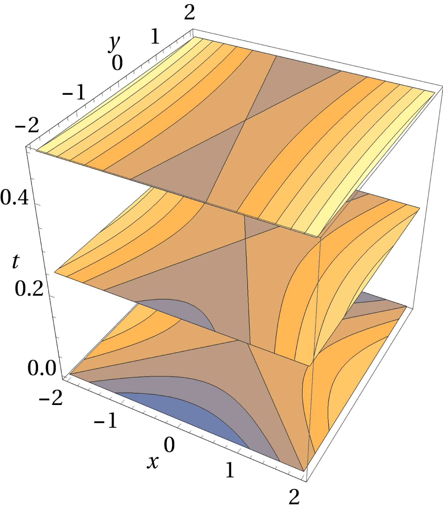
Figure 2. Flux surfaces near magnetic null for (4.2) at a fixed longitudinal coordinate $z=0$
, with
$z=0$
, with $a=1$
,
$a=1$
, $b=0.5$
,
$b=0.5$
, $\unicode[STIX]{x1D6E4}=1$
and
$\unicode[STIX]{x1D6E4}=1$
and $z_{0}=1$
.
$z_{0}=1$
.
As a second example, by choosing $\unicode[STIX]{x1D6E9}=(z-v_{A}t)/z_{0}$
, we find a solution which, at time
$\unicode[STIX]{x1D6E9}=(z-v_{A}t)/z_{0}$
, we find a solution which, at time $t=0$
, is in the same helical configuration as (4.2), but now moves along the guide field at the Alfvén speed.
$t=0$
, is in the same helical configuration as (4.2), but now moves along the guide field at the Alfvén speed.
5 Symmetry analysis
5.1 Infinitesimal generators
The maps given in § 3 can be viewed geometrically as a continuous family of transformations of the graph of the solution, which is a set of points in the (ten-dimensional) space labelled by $(v,x,y,z,t;\unicode[STIX]{x1D719},\unicode[STIX]{x1D713},\unicode[STIX]{x1D6FF}n,\unicode[STIX]{x1D6FF}T,g)$
. These subgroups of transformations can be characterized by their infinitesimal generators
$(v,x,y,z,t;\unicode[STIX]{x1D719},\unicode[STIX]{x1D713},\unicode[STIX]{x1D6FF}n,\unicode[STIX]{x1D6FF}T,g)$
. These subgroups of transformations can be characterized by their infinitesimal generators $\unicode[STIX]{x1D729}$
.
$\unicode[STIX]{x1D729}$
.
For example, consider the action of an infinitesimal gauge transformation $\unicode[STIX]{x1D6FF}H(z,t)$
on the graph of a solution
$\unicode[STIX]{x1D6FF}H(z,t)$
on the graph of a solution $(\unicode[STIX]{x1D719},\unicode[STIX]{x1D713},\unicode[STIX]{x1D6FF}n,\unicode[STIX]{x1D6FF}T,g)$
:
$(\unicode[STIX]{x1D719},\unicode[STIX]{x1D713},\unicode[STIX]{x1D6FF}n,\unicode[STIX]{x1D6FF}T,g)$
:
 $$\begin{eqnarray}\displaystyle \displaystyle (\tilde{v},\tilde{\boldsymbol{x}}_{\bot },\tilde{z},\tilde{t},\tilde{\unicode[STIX]{x1D719}},\tilde{\unicode[STIX]{x1D713}},\tilde{\unicode[STIX]{x1D6FF}n},\tilde{\unicode[STIX]{x1D6FF}T},\tilde{g}) & = & \displaystyle [1-\unicode[STIX]{x1D6FF}H_{t}\unicode[STIX]{x2202}_{\unicode[STIX]{x1D719}}+\unicode[STIX]{x1D6FF}H_{z}\unicode[STIX]{x2202}_{\unicode[STIX]{x1D713}}+\mathit{O}(\unicode[STIX]{x1D6FF}^{2})]\nonumber\\ \displaystyle \displaystyle & & \displaystyle \times \,(v,\boldsymbol{x},z,t;\unicode[STIX]{x1D719},\unicode[STIX]{x1D713},\unicode[STIX]{x1D6FF}n,\unicode[STIX]{x1D6FF}T,g).\end{eqnarray}$$
Here, the infinitesimal generator is seen to be
 $$\begin{eqnarray}\displaystyle & \displaystyle \unicode[STIX]{x1D729}_{H}=-H_{t}\unicode[STIX]{x2202}_{\unicode[STIX]{x1D719}}+H_{z}\unicode[STIX]{x2202}_{\unicode[STIX]{x1D713}}. & \displaystyle\end{eqnarray}$$
Similarly, the infinitesimal generators for (3.3) and (3.5) are
 $$\begin{eqnarray}\displaystyle & \displaystyle \unicode[STIX]{x1D729}_{\unicode[STIX]{x1D743}}=-\unicode[STIX]{x1D743}\boldsymbol{\cdot }\unicode[STIX]{x2202}_{\boldsymbol{x}_{\bot }}+\unicode[STIX]{x2202}_{z}\hat{\boldsymbol{z}}\boldsymbol{\cdot }\unicode[STIX]{x1D743}\times \boldsymbol{x}_{\bot }\unicode[STIX]{x2202}_{\unicode[STIX]{x1D713}}-\unicode[STIX]{x2202}_{t}\hat{\boldsymbol{z}}\boldsymbol{\cdot }\unicode[STIX]{x1D743}\times \boldsymbol{x}_{\bot }\unicode[STIX]{x2202}_{\unicode[STIX]{x1D719}}, & \displaystyle\end{eqnarray}$$
and
 $$\begin{eqnarray}\displaystyle \displaystyle \unicode[STIX]{x1D729}_{\unicode[STIX]{x1D6E9}} & = & \displaystyle \unicode[STIX]{x1D6E9}\unicode[STIX]{x2202}_{\unicode[STIX]{x1D703}}+\unicode[STIX]{x2202}_{z}\left({\displaystyle \frac{r^{2}}{2}}\unicode[STIX]{x1D6E9}\right)\unicode[STIX]{x2202}_{\unicode[STIX]{x1D713}}+\left[-\unicode[STIX]{x2202}_{t}\left({\displaystyle \frac{r^{2}}{2}}\unicode[STIX]{x1D6E9}\right)+{\mathcal{F}}\right]\unicode[STIX]{x2202}_{\unicode[STIX]{x1D719}}\nonumber\\ \displaystyle & & \displaystyle +\,\left[-v_{A}^{-2}\unicode[STIX]{x0394}\unicode[STIX]{x2202}_{t}\left({\displaystyle \frac{r^{2}}{2}}\unicode[STIX]{x1D6E9}\right)\right]\unicode[STIX]{x2202}_{\unicode[STIX]{x1D6FF}n}+{\mathcal{T}}\unicode[STIX]{x2202}_{\unicode[STIX]{x1D6FF}T}+G\unicode[STIX]{x2202}_{g},\end{eqnarray}$$
respectively.
There is a one-to-one correspondence between Lie-group transformations and their infinitesimal generators. For a rigorous but readable introduction to this formalism, see Olver (Reference Olver1993, chapter 1).
5.2 Generators acting on differential equations
As an extension to a standard graph, one can take a solution of the ZS model and produce a graph in the higher-dimensional space consisting of the independent and dependent variables, as well as all higher derivatives up to second order (the highest order that appears in the model equations). In this higher-dimensional jet space, labelled $(v,x,y,z,t;\unicode[STIX]{x1D719},\unicode[STIX]{x1D713},\unicode[STIX]{x1D6FF}n,\unicode[STIX]{x1D6FF}T,g;\unicode[STIX]{x1D719}_{v},\ldots ,\unicode[STIX]{x1D719}_{t},\ldots )\equiv (x^{i},u^{\unicode[STIX]{x1D6FC}},u_{i}^{\unicode[STIX]{x1D6FC}},u_{i,j}^{\unicode[STIX]{x1D6FC}})$
, the action of a symmetry transformation will also involve the coordinates associated with the derivatives:
$(v,x,y,z,t;\unicode[STIX]{x1D719},\unicode[STIX]{x1D713},\unicode[STIX]{x1D6FF}n,\unicode[STIX]{x1D6FF}T,g;\unicode[STIX]{x1D719}_{v},\ldots ,\unicode[STIX]{x1D719}_{t},\ldots )\equiv (x^{i},u^{\unicode[STIX]{x1D6FC}},u_{i}^{\unicode[STIX]{x1D6FC}},u_{i,j}^{\unicode[STIX]{x1D6FC}})$
, the action of a symmetry transformation will also involve the coordinates associated with the derivatives:
 $$\begin{eqnarray}\displaystyle & \displaystyle \unicode[STIX]{x1D729}_{\ast }=\underbrace{\unicode[STIX]{x1D709}^{i}(x,u)\unicode[STIX]{x2202}_{x^{i}}+U^{\unicode[STIX]{x1D6FC}}(x,u)\unicode[STIX]{x2202}_{u^{\unicode[STIX]{x1D6FC}}}}_{=\unicode[STIX]{x1D729}}+\mathop{\sum }_{i,j}U^{\unicode[STIX]{x1D6FC};i,j}(x,u)\unicode[STIX]{x2202}_{u_{ij}^{\unicode[STIX]{x1D6FC}}}. & \displaystyle\end{eqnarray}$$
In this higher-dimensional space, the model equations, generically expressed in the form
 $$\begin{eqnarray}\displaystyle & \displaystyle F(x^{i},u^{\unicode[STIX]{x1D6FC}},u_{i}^{\unicode[STIX]{x1D6FC}},u_{i,j}^{\unicode[STIX]{x1D6FC}})=0\quad \text{for all }x^{i}, & \displaystyle\end{eqnarray}$$
are formally algebraic equations.
A transformation generated by (5.2) is a symmetry of the model if the model equations themselves are invariant under the transformation while transforming a solution. That is
 $$\begin{eqnarray}\displaystyle & \displaystyle \unicode[STIX]{x1D729}_{\ast }F=0\text{ whenever }F=0\Leftrightarrow \unicode[STIX]{x1D729}\text{is a symmetry of }F. & \displaystyle\end{eqnarray}$$
This invariance criterion is a fundamental theorem in symmetry analysis of differential equations.
The second key result is the prolongation formula, which expresses the functions $U^{\unicode[STIX]{x1D6FC};i,j}$
in terms of the
$U^{\unicode[STIX]{x1D6FC};i,j}$
in terms of the $U^{\unicode[STIX]{x1D6FC}}$
and
$U^{\unicode[STIX]{x1D6FC}}$
and $\unicode[STIX]{x1D709}^{i}$
. In other words, given an infinitesimal generator
$\unicode[STIX]{x1D709}^{i}$
. In other words, given an infinitesimal generator $\unicode[STIX]{x1D729}$
in the space
$\unicode[STIX]{x1D729}$
in the space $(x^{i},u^{\unicode[STIX]{x1D6FC}})$
, the prolongation formula provides an explicit expression of the form of the generator
$(x^{i},u^{\unicode[STIX]{x1D6FC}})$
, the prolongation formula provides an explicit expression of the form of the generator $\unicode[STIX]{x1D729}_{\ast }$
in the jet space
$\unicode[STIX]{x1D729}_{\ast }$
in the jet space $(x^{i},u^{\unicode[STIX]{x1D6FC}},u_{i}^{\unicode[STIX]{x1D6FC}},u_{ij}^{\unicode[STIX]{x1D6FC}})$
.
$(x^{i},u^{\unicode[STIX]{x1D6FC}},u_{i}^{\unicode[STIX]{x1D6FC}},u_{ij}^{\unicode[STIX]{x1D6FC}})$
.
Using the prolongation formula, the invariance criterion (5.7) becomes a working procedure to obtain symmetries. Starting from the general symmetry generator
 $$\begin{eqnarray}\displaystyle & \displaystyle \unicode[STIX]{x1D729}=\unicode[STIX]{x1D709}^{i}(x,u)\unicode[STIX]{x2202}_{x^{i}}+U^{\unicode[STIX]{x1D6FC}}(x,u)\unicode[STIX]{x2202}_{u^{\unicode[STIX]{x1D6FC}}}, & \displaystyle\end{eqnarray}$$
with unknown coefficients $\unicode[STIX]{x1D709}^{i}$
and
$\unicode[STIX]{x1D709}^{i}$
and $U^{\unicode[STIX]{x1D6FC}}$
, one uses the prolongation formula to compute the form of this symmetry generator (denoted here as
$U^{\unicode[STIX]{x1D6FC}}$
, one uses the prolongation formula to compute the form of this symmetry generator (denoted here as $\unicode[STIX]{x1D729}_{\ast }$
) in jet space. Once this is computed, the invariance criterion imposes conditions on the coefficients of
$\unicode[STIX]{x1D729}_{\ast }$
) in jet space. Once this is computed, the invariance criterion imposes conditions on the coefficients of $\unicode[STIX]{x1D729}_{\ast }$
which must be satisfied in order for (5.8) to correspond to a symmetry of the system. By solving these determining equations, the most general symmetry of the form (5.8) is obtained.
$\unicode[STIX]{x1D729}_{\ast }$
which must be satisfied in order for (5.8) to correspond to a symmetry of the system. By solving these determining equations, the most general symmetry of the form (5.8) is obtained.
There are two characteristics of this procedure that will be leveraged to extend the procedure to the ZS model, which also has integral relations. First, in a model consisting of more than one equation, the invariance criterion can be applied to one equation at a time. After all, any symmetry of the full model must leave each of its equations unchanged (on the space of solutions of the model). Thus we can find the symmetries of the under-determined system (2.28)–(2.30) before considering the integral relations (2.31) and (2.33).
The second noteworthy point is that determining equations are usually straightforward to solve, even for highly complicated nonlinear models, provided there are no integral terms. This justifies the operation of deriving the (generally more complicated) symmetry group of the under-determined model first. Once the symmetry group of the under-determined model is obtained, this class of transformations is used to simplify application of the integral constraints.
5.3 Determining equations
We begin our analysis with a generator of the form
 $$\begin{eqnarray}\displaystyle & \displaystyle \unicode[STIX]{x1D729}=\unicode[STIX]{x1D709}^{(t)}\unicode[STIX]{x2202}_{t}+\unicode[STIX]{x1D709}^{(z)}\unicode[STIX]{x2202}_{z}+X\unicode[STIX]{x2202}_{x}+Y\unicode[STIX]{x2202}_{y}+\unicode[STIX]{x1D6F7}\unicode[STIX]{x2202}_{\unicode[STIX]{x1D719}}+\unicode[STIX]{x1D6F9}\unicode[STIX]{x2202}_{\unicode[STIX]{x1D713}}+G\unicode[STIX]{x2202}_{g}+{\mathcal{T}}\unicode[STIX]{x2202}_{\unicode[STIX]{x1D6FF}T}+N\unicode[STIX]{x2202}_{\unicode[STIX]{x1D6FF}n}, & \displaystyle\end{eqnarray}$$
where $\unicode[STIX]{x1D709}^{(a)}$
are constants, and the remaining unknown functions depend only on the independent variables. This is not the most general form. Our motivation for choosing this simpler but less general form is based on exploratory computational analysis, using software provided by Cantwell (Reference Cantwell2002). This exploration suggests that all of the symmetries are of the form (5.9).
$\unicode[STIX]{x1D709}^{(a)}$
are constants, and the remaining unknown functions depend only on the independent variables. This is not the most general form. Our motivation for choosing this simpler but less general form is based on exploratory computational analysis, using software provided by Cantwell (Reference Cantwell2002). This exploration suggests that all of the symmetries are of the form (5.9).
5.3.1 Local determining equations
Following the procedure sketched in the preceding subsection, we obtain from (2.28) and (2.30) the following determining equations:
 $$\begin{eqnarray}\displaystyle & \displaystyle X_{v}=Y_{v}=\unicode[STIX]{x1D6F7}_{v}=\unicode[STIX]{x1D6F9}_{v}=T_{v}=N_{v}=0, & \displaystyle\end{eqnarray}$$
 $$\begin{eqnarray}\displaystyle & \displaystyle X_{x}+Y_{y}=0, & \displaystyle\end{eqnarray}$$
 $$\begin{eqnarray}\displaystyle & \displaystyle X_{x}=Y_{y}=0, & \displaystyle\end{eqnarray}$$
 $$\begin{eqnarray}\displaystyle & \displaystyle \unicode[STIX]{x1D6F9}_{x}-Y_{z}=\unicode[STIX]{x1D6F9}_{y}-X_{z}=0, & \displaystyle\end{eqnarray}$$
 $$\begin{eqnarray}\displaystyle & \displaystyle \unicode[STIX]{x1D6F7}_{y}+X_{t}=\unicode[STIX]{x1D6F7}_{x}-Y_{t}=0, & \displaystyle\end{eqnarray}$$
 $$\begin{eqnarray}\displaystyle & \displaystyle N_{x}=N_{y}=0, & \displaystyle\end{eqnarray}$$
 $$\begin{eqnarray}\displaystyle & \displaystyle {\mathcal{T}}_{x}={\mathcal{T}}_{y}=0, & \displaystyle\end{eqnarray}$$
 $$\begin{eqnarray}\displaystyle & \displaystyle G_{x}=G_{y}=0, & \displaystyle\end{eqnarray}$$
 $$\begin{eqnarray}\displaystyle & \displaystyle N_{t}=\unicode[STIX]{x0394}\unicode[STIX]{x1D6F9}_{z}, & \displaystyle\end{eqnarray}$$
 $$\begin{eqnarray}\displaystyle & \displaystyle \unicode[STIX]{x1D6F9}_{t}-\unicode[STIX]{x0394}\unicode[STIX]{x1D6F9}_{t}=\unicode[STIX]{x0394}\unicode[STIX]{x1D6F9}-\unicode[STIX]{x1D6F7}_{z}-N_{z}-{\mathcal{T}}_{z}, & \displaystyle\end{eqnarray}$$
 $$\begin{eqnarray}\displaystyle & \displaystyle G_{t}+v(G_{z}+{\mathcal{T}})=G_{vv}-vG_{v}+(1-v^{2})(N_{t}+{\mathcal{T}}). & \displaystyle\end{eqnarray}$$
These linear differential equations are sometimes called the ‘local’ determining equations; symmetries of the non-local, integral relations (2.31)–(2.33) remain to be considered.
5.3.2 Integral determining equations
For integro-differential equations, the notion of the jet space (itself a generalization of the graph space) can be extended to include the moments of independent variables which appear in the model. We denote the variables in this space generically as $(x^{i},u^{\unicode[STIX]{x1D6FC}},u_{i}^{\unicode[STIX]{x1D6FC}},u_{i,j}^{\unicode[STIX]{x1D6FC}},m^{\unicode[STIX]{x1D707}}\equiv \int \!K_{\unicode[STIX]{x1D6FC}}^{\unicode[STIX]{x1D707}}(x,x^{\prime })u^{\unicode[STIX]{x1D6FC}}(x^{\prime }))$
. For the ZS model, the two moment variables are
$(x^{i},u^{\unicode[STIX]{x1D6FC}},u_{i}^{\unicode[STIX]{x1D6FC}},u_{i,j}^{\unicode[STIX]{x1D6FC}},m^{\unicode[STIX]{x1D707}}\equiv \int \!K_{\unicode[STIX]{x1D6FC}}^{\unicode[STIX]{x1D707}}(x,x^{\prime })u^{\unicode[STIX]{x1D6FC}}(x^{\prime }))$
. For the ZS model, the two moment variables are $\unicode[STIX]{x1D6FF}n$
and
$\unicode[STIX]{x1D6FF}n$
and $\unicode[STIX]{x1D6FF}T$
. What is needed for the invariance criterion (5.7) is the expression for
$\unicode[STIX]{x1D6FF}T$
. What is needed for the invariance criterion (5.7) is the expression for $\unicode[STIX]{x1D729}m^{\unicode[STIX]{x1D707}}$
in terms of the generator coefficients
$\unicode[STIX]{x1D729}m^{\unicode[STIX]{x1D707}}$
in terms of the generator coefficients $U^{\unicode[STIX]{x1D6FC}}$
and
$U^{\unicode[STIX]{x1D6FC}}$
and $X^{i}$
.
$X^{i}$
.
For this purpose, there is a very useful fact: one can re-express $\unicode[STIX]{x1D729}$
in canonical form, where it acts only on the dependent variables:
$\unicode[STIX]{x1D729}$
in canonical form, where it acts only on the dependent variables:
 $$\begin{eqnarray}\displaystyle & \displaystyle \unicode[STIX]{x1D729}=\mathop{\sum }_{\unicode[STIX]{x1D6FC}}Q^{\unicode[STIX]{x1D6FC}}\unicode[STIX]{x2202}_{u^{\unicode[STIX]{x1D6FC}}}, & \displaystyle\end{eqnarray}$$
with
 $$\begin{eqnarray}\displaystyle & \displaystyle Q^{\unicode[STIX]{x1D6FC}}=U^{\unicode[STIX]{x1D6FC}}-\mathop{\sum }_{i}X^{i}u_{i}^{\unicode[STIX]{x1D6FC}}. & \displaystyle\end{eqnarray}$$
It turns out (see e.g. Kovalev et al.
Reference Kovalev, Krivenko and Pustovalev1996) that the action of the canonical generator (5.21) on an integral – a functional of the $u^{\unicode[STIX]{x1D6FC}}$
– is obtained by replacing ordinary derivatives by functional derivatives in the canonical expression
$u^{\unicode[STIX]{x1D6FC}}$
– is obtained by replacing ordinary derivatives by functional derivatives in the canonical expression
 $$\begin{eqnarray}\displaystyle & \displaystyle \unicode[STIX]{x1D729}m^{\unicode[STIX]{x1D707}}=\mathop{\sum }_{\unicode[STIX]{x1D6FC}}Q^{\unicode[STIX]{x1D6FC}}\int \text{d}x^{\prime }{\displaystyle \frac{\unicode[STIX]{x1D6FF}m^{\unicode[STIX]{x1D707}}}{\unicode[STIX]{x1D6FF}u^{\unicode[STIX]{x1D6FC}}(x^{\prime })}}. & \displaystyle\end{eqnarray}$$
Using (5.23), the invariance criteria $\unicode[STIX]{x1D729}$
(2.31)
$\unicode[STIX]{x1D729}$
(2.31) $=0$
and
$=0$
and $\unicode[STIX]{x1D729}$
(2.33)
$\unicode[STIX]{x1D729}$
(2.33) $=0$
give the integral determining equations
$=0$
give the integral determining equations
 $$\begin{eqnarray}\displaystyle & \displaystyle {\mathcal{T}}={\displaystyle \frac{1}{\sqrt{2\unicode[STIX]{x03C0}}}}\int \text{d}v^{\prime }{v^{\prime }}^{2}\text{e}^{-{v^{\prime }}^{2}/2}G(v^{\prime }), & \displaystyle\end{eqnarray}$$
and
 $$\begin{eqnarray}\displaystyle & \displaystyle N=\hat{{\mathcal{G}}}\unicode[STIX]{x1D6F7}, & \displaystyle\end{eqnarray}$$
respectively. Similarly, the integral constraints (2.32) lead to the determining equations
 $$\begin{eqnarray}\displaystyle & \displaystyle \left(\begin{array}{@{}c@{}}0\\ 0\end{array}\right)={\displaystyle \frac{1}{\sqrt{2\unicode[STIX]{x03C0}}}}\int \text{d}v^{\prime }\left(\begin{array}{@{}c@{}}1\\ v^{\prime }\end{array}\right)\text{e}^{-{v^{\prime }}^{2}/2}G(v^{\prime }). & \displaystyle\end{eqnarray}$$
Thus our full system of equations for the generator coefficients consists of the local equations (5.11)–(5.20) together with the integral relations (5.24)–(5.26). Note in particular that this system of equations also involves a gyroaveraging operator, as well as other integral relations which usually lead to analytical intractability. However, in this case, the local determining equations form an autonomous subsystem; we are able to obtain their general solution before even deriving the remaining (integral) determining equations.
5.4 Solution of determining equations
The general solution of the local determining equations (5.10)–(5.20) is
 $$\begin{eqnarray}\displaystyle & \displaystyle X=\unicode[STIX]{x1D6E9}y+\hat{\boldsymbol{x}}\boldsymbol{\cdot }\unicode[STIX]{x1D743}, & \displaystyle\end{eqnarray}$$
 $$\begin{eqnarray}\displaystyle & \displaystyle Y=-\unicode[STIX]{x1D6E9}x+\hat{\boldsymbol{y}}\boldsymbol{\cdot }\unicode[STIX]{x1D743}, & \displaystyle\end{eqnarray}$$
 $$\begin{eqnarray}\displaystyle & \displaystyle \unicode[STIX]{x1D6F9}=\unicode[STIX]{x2202}_{z}\left(\unicode[STIX]{x1D6E9}{\displaystyle \frac{x^{2}+y^{2}}{2}}+\hat{\boldsymbol{z}}\boldsymbol{\cdot }\unicode[STIX]{x1D743}\times \boldsymbol{x}_{\bot }+H\right), & \displaystyle\end{eqnarray}$$
 $$\begin{eqnarray}\displaystyle & \displaystyle \unicode[STIX]{x1D6F7}=-\unicode[STIX]{x2202}_{t}\left(\unicode[STIX]{x1D6E9}{\displaystyle \frac{x^{2}+y^{2}}{2}}+\hat{\boldsymbol{z}}\boldsymbol{\cdot }\unicode[STIX]{x1D743}\times \boldsymbol{x}_{\bot }+H\right)+[2(\unicode[STIX]{x1D6E9}_{t}+\unicode[STIX]{x1D6E9})+{\mathcal{T}}+N], & \displaystyle\end{eqnarray}$$
 $$\begin{eqnarray}\displaystyle & \displaystyle N=-2v_{A}^{-2}\unicode[STIX]{x1D6E9}_{t} & \displaystyle\end{eqnarray}$$
 $$\begin{eqnarray}\displaystyle & \displaystyle {\mathcal{T}}={\mathcal{T}}(z,t), & \displaystyle\end{eqnarray}$$
 $$\begin{eqnarray}\displaystyle & \displaystyle G_{t}+vG_{z}=-G_{vv}+vG_{v}-(1-v^{2})(N_{t}+{\mathcal{T}})-vT_{z}. & \displaystyle\end{eqnarray}$$
Here $\hat{\boldsymbol{x}}\boldsymbol{\cdot }\unicode[STIX]{x1D743}(z,t)$
,
$\hat{\boldsymbol{x}}\boldsymbol{\cdot }\unicode[STIX]{x1D743}(z,t)$
, $\hat{\boldsymbol{y}}\boldsymbol{\cdot }\unicode[STIX]{x1D743}(z,t)$
and
$\hat{\boldsymbol{y}}\boldsymbol{\cdot }\unicode[STIX]{x1D743}(z,t)$
and $H(z,t)$
are arbitrary functions, while
$H(z,t)$
are arbitrary functions, while $\unicode[STIX]{x1D6E9}(z,t)$
is an arbitrary solution to the wave equation (3.4).
$\unicode[STIX]{x1D6E9}(z,t)$
is an arbitrary solution to the wave equation (3.4).
In obtaining this result, we have used
 $$\begin{eqnarray}\displaystyle \displaystyle \hat{{\mathcal{G}}}\unicode[STIX]{x1D6F7} & = & \displaystyle {\displaystyle \frac{1}{v_{A}^{2}}}\unicode[STIX]{x0394}\unicode[STIX]{x1D6F7},\end{eqnarray}$$
 $$\begin{eqnarray}\displaystyle & = & \displaystyle -{\displaystyle \frac{2}{v_{A}^{2}}}\unicode[STIX]{x1D6E9}_{t}.\end{eqnarray}$$
In other words, the leading FLR approximation to $\hat{{\mathcal{G}}}$
, shown in (2.38), here becomes exact, since the
$\hat{{\mathcal{G}}}$
, shown in (2.38), here becomes exact, since the $\unicode[STIX]{x1D6F7}$
given in (5.30) is quadratic in the perpendicular coordinates.
$\unicode[STIX]{x1D6F7}$
given in (5.30) is quadratic in the perpendicular coordinates.
The function $G$
is determined implicitly by (5.33) and constrained to satisfy
$G$
is determined implicitly by (5.33) and constrained to satisfy
 $$\begin{eqnarray}\displaystyle & \displaystyle 0=\int \text{d}v^{\prime }\,G(v^{\prime })\text{e}^{-{v^{\prime }}^{2}/2}, & \displaystyle\end{eqnarray}$$
 $$\begin{eqnarray}\displaystyle & \displaystyle 0=\int \text{d}v^{\prime }\,v^{\prime }G(v^{\prime })\text{e}^{-{v^{\prime }}^{2}/2}. & \displaystyle\end{eqnarray}$$
The symmetries discussed in § 3 follow from equations (5.27)–(5.37).
6 Conclusion
We have found that the fluid-gyrokinetic ZS model has a rich symmetry group, with the full set of symmetries spanned by five arbitrary functions $H(z,t)$
,
$H(z,t)$
, $\hat{\boldsymbol{x}}\boldsymbol{\cdot }\unicode[STIX]{x1D743}(z,t)$
,
$\hat{\boldsymbol{x}}\boldsymbol{\cdot }\unicode[STIX]{x1D743}(z,t)$
, $\hat{\boldsymbol{y}}\boldsymbol{\cdot }\unicode[STIX]{x1D743}(z,t)$
and
$\hat{\boldsymbol{y}}\boldsymbol{\cdot }\unicode[STIX]{x1D743}(z,t)$
and $\unicode[STIX]{x1D6E9}^{\pm }(z\pm v_{A}t)$
, and the two constants
$\unicode[STIX]{x1D6E9}^{\pm }(z\pm v_{A}t)$
, and the two constants $\unicode[STIX]{x1D709}^{(z)}$
and
$\unicode[STIX]{x1D709}^{(z)}$
and $\unicode[STIX]{x1D709}^{(t)}$
, corresponding to translations in
$\unicode[STIX]{x1D709}^{(t)}$
, corresponding to translations in $z$
and
$z$
and $t$
. These symmetries are discussed in § 3, and summarized by (5.9), with (5.27)–(5.37).
$t$
. These symmetries are discussed in § 3, and summarized by (5.9), with (5.27)–(5.37).
To our knowledge, this is the first time symmetry analysis has been applied to a model with a gyroaveraging operator. Gyroaveraging, viewed as a constitutive relation linking $\unicode[STIX]{x1D719}$
to
$\unicode[STIX]{x1D719}$
to $\unicode[STIX]{x1D6FF}n$
, turns out to not pose a serious obstacle in our analysis, largely because the
$\unicode[STIX]{x1D6FF}n$
, turns out to not pose a serious obstacle in our analysis, largely because the $x_{\bot }$
dependence of the infinitesimal generator for
$x_{\bot }$
dependence of the infinitesimal generator for $\unicode[STIX]{x1D719}$
allowed the exact gyroaverage to be expressed in closed form. Similarly, the generator
$\unicode[STIX]{x1D719}$
allowed the exact gyroaverage to be expressed in closed form. Similarly, the generator $G$
for displacement symmetry of the distribution function is found to satisfy exactly a linear drift-kinetic equation. The success of symmetry analysis for the ZS model suggests that a similar study for the full gyrokinetic equations might also be possible.
$G$
for displacement symmetry of the distribution function is found to satisfy exactly a linear drift-kinetic equation. The success of symmetry analysis for the ZS model suggests that a similar study for the full gyrokinetic equations might also be possible.
Our analysis assumes, based on computational exploration, a special form for the symmetries, so it is possible that additional symmetries remain undiscovered. In fact, even if we did begin our analysis with the most general possible transformation, the integral terms in ZS place it beyond the scope of the theorems that would prove completeness. Our analysis also excludes consideration of the discrete symmetries, such as transforming to a left-handed coordinate system: $x\rightarrow y,y\rightarrow -x$
. The most general symmetry group of the model is obtained by composing the connected Lie subgroup, which is obtained by exponentiating the infinitesimal generators, with the discrete subgroup of symmetry transformations admitted by the model. Rigorous methods exist for finding the discrete symmetries of differential equations, but they are generally limited in scope and can require the solution of complicated determining equations (Gaeta & Rodríguez Reference Gaeta and Rodríguez1996). We save this complementary analysis for future work.
$x\rightarrow y,y\rightarrow -x$
. The most general symmetry group of the model is obtained by composing the connected Lie subgroup, which is obtained by exponentiating the infinitesimal generators, with the discrete subgroup of symmetry transformations admitted by the model. Rigorous methods exist for finding the discrete symmetries of differential equations, but they are generally limited in scope and can require the solution of complicated determining equations (Gaeta & Rodríguez Reference Gaeta and Rodríguez1996). We save this complementary analysis for future work.
Because RMHD is a limit of the ZS model, our analysis also provides a large family of symmetries of RMHD. RMHD is a simpler and better studied model, so there are more exact solutions available to transform by our methods. In particular, the results obtained here can be used to generate new exact solutions to RMHD by transforming the Elsasser solutions (Elsasser Reference Elsasser1950), which play an important role in MHD theories of turbulence (for a review, see, e.g. Biskamp Reference Biskamp2003).
For illustrative purposes, the modified Chapman–Kendall solution obtained in § 4.2 employed a very simple particular symmetry transformation. More generally, using the full set of transformations obtained here, the original two parameter Chapman–Kendall solution becomes a large family of solutions, spanned by the arbitrary functions $H$
,
$H$
, $\unicode[STIX]{x1D743}$
and
$\unicode[STIX]{x1D743}$
and $\unicode[STIX]{x1D6E9}$
.
$\unicode[STIX]{x1D6E9}$
.
In the context of the full kinetic model, one can, for example, leverage simulation results that start from a Chapman–Kendall-like two-dimensional current configuration to infer the behaviour of a whole family of (generally three-dimensional) initial current profiles, such as the helical collapsing current sheet given in (4.2).
Noether’s theorem applies to all of the symmetry transformations obtained here. If one is able to construct an action for this model (see Charidakos et al. Reference Charidakos, Lingam, Morrison, White and Wurm2014; Morrison, Lingam & Acevedo Reference Morrison, Lingam and Acevedo2014; Burby Reference Burby2017, for manifestly action-preserving derivations of reduced models), and if the action is invariant under any of these transformations, then one can use Noether’s theorem to derive conserved quantities which, like the symmetries themselves, may not be obvious from physical considerations. Symmetry analysis can thus enhance the value of a reduced model by uncovering quantities which, while perhaps not exactly conserved in the full Maxwell–Boltzmann description, are approximately constant in particular regimes of interest. For the ZS model, this context would be nonlinear fluctuations in a high temperature strongly magnetized plasma.
Acknowledgements
R.L.W. was supported by the U.S. Department of Energy Fusion Energy Sciences Postdoctoral Research Program administered by the Oak Ridge Institute for Science and Education (ORISE) for the DOE. ORISE is managed by Oak Ridge Associated Universities (ORAU) under DOE contract number DE-SC0014664. All opinions expressed in this paper are the author’s and do not necessarily reflect the policies and views of DOE, ORAU, or ORISE. The work of R.D.H. was funded by the U.S. Department of Energy under contract no. DE-FG02-04ER-54742 and by The University of Texas at Austin. N.F.L. was partially funded by US Department of Energy grant no. DE-FG02-91ER54109. We also acknowledge the use of Brian Cantwell’s Lie-group software, implemented on Mathematica®.


