


1 Introduction
The Crab Nebula is an iconic astronomical object with an exceptionally long research history going back to the observations of a ‘guest star’ by Chinese astronomers in 1054. Astronomical studies of the nebula have proved to be an exceptionally fruitful both for discovering new space phenomena and for developing of their physical models. As we now know, the nebula has a lot in common with many other cosmic objects, such as AGN jets, gamma-ray bursts, gamma-ray binaries etc. and the knowledge gained from its study has found numerous applications in many other areas of astrophysics.
It is now well established that the nebula is a result of the interaction between the magnetised ultra-relativistic wind from the Crab pulsar and the supernova shell ejected during the 1054 explosion. The physical models of this interaction have evolved from simplified spherically symmetric one-dimensional (1-D) analytic models (Rees & Gunn Reference Rees and Gunn1974; Kennel & Coroniti Reference Kennel and Coroniti1984a ) through early axisymmetric numerical models (Del Zanna, Amato & Bucciantini Reference Del Zanna, Amato and Bucciantini2004; Komissarov & Lyubarsky Reference Komissarov and Lyubarsky2004; Lyutikov, Komissarov & Porth Reference Lyutikov, Komissarov and Porth2016) to fully 3-D sophisticated numerical simulations (Porth, Komissarov & Keppens Reference Porth, Komissarov and Keppens2013; Olmi et al. Reference Olmi, Del Zanna, Amato, Bucciantini and Mignone2016). The current fluid models seem to explain many of both the large scale and fine features of the nebula quite convincingly but there are still many uncertainties. The most important of these concerns the origin of the high-energy leptons producing the observed non-thermal emission of the nebula.
Following the pioneering work by Rees & Gunn (Reference Rees and Gunn1974) and Kennel & Coroniti (Reference Kennel and Coroniti1984b
), it is usually assumed that these particles are accelerated at the termination shock of the pulsar wind. This assumption seems rather natural given the success of the particle acceleration theory for non-relativistic shocks (e.g., Riquelme & Spitkovsky Reference Riquelme and Spitkovsky2011). However, in the case of pulsar winds we are dealing with relativistic shocks, which are much less promising as particle accelerators in the presence of a large-scale magnetic field. According to the recent particle-in-cell (PIC) simulations (Sironi & Spitkovsky Reference Sironi and Spitkovsky2009) this acceleration mechanism operates only for very low magnetisation of the upstream plasma (
 $\unicode[STIX]{x1D70E}<10^{-3}$
, where
$\unicode[STIX]{x1D70E}<10^{-3}$
, where
 $\unicode[STIX]{x1D70E}$
is the plasma magnetization parameter (Kennel & Coroniti Reference Kennel and Coroniti1984a
; Spitkovsky Reference Spitkovsky, Bulik, Rudak and Madejski2005; Sironi & Spitkovsky Reference Sironi and Spitkovsky2009)).
$\unicode[STIX]{x1D70E}$
is the plasma magnetization parameter (Kennel & Coroniti Reference Kennel and Coroniti1984a
; Spitkovsky Reference Spitkovsky, Bulik, Rudak and Madejski2005; Sironi & Spitkovsky Reference Sironi and Spitkovsky2009)).
Unfortunately, the magnetisation of pulsar winds cannot be measured directly and we have to deal with indirect estimates and theoretical predictions only. These do not always go hand in hand. Thus the theory of pulsar magnetospheres and ideal MHD winds predict very high magnetisation of pulsar winds whereas the original spherically symmetric model of the Crab Nebula fits the data only if the magnetisation is very low. This controversy is known as the
 $\unicode[STIX]{x1D70E}$
-problem. Interestingly, the magnetisation deduced by Kennel & Coroniti (Reference Kennel and Coroniti1984a
) marginally satisfies the above condition of the shock acceleration mechanism.
$\unicode[STIX]{x1D70E}$
-problem. Interestingly, the magnetisation deduced by Kennel & Coroniti (Reference Kennel and Coroniti1984a
) marginally satisfies the above condition of the shock acceleration mechanism.
The brightest and the most compact resolved feature of the Crab Nebula is the so-called inner knot located within one arcsec from the Crab pulsar. A similar knot was found in the synthetic images of the Crab Nebula based on the low-
 $\unicode[STIX]{x1D70E}$
wind models (Komissarov & Lyubarsky Reference Komissarov and Lyubarsky2004), where it was identified with Doppler-boosted emission of the termination shock. Yuan & Blandford (Reference Yuan and Blandford2015) and Lyutikov et al. (Reference Lyutikov, Komissarov and Porth2016) explored the shock model of the knot in detail and concluded that it is consistent with the observations only if the downstream plasma magnetisation is low. For an ideal fast magnetosonic shock, this also means low upstream magnetisation. If however the upstream magnetic field is highly inhomogeneous things can be rather different. In this case, the shock can trigger rapid magnetic dissipation immediately downstream of the ideal shock and the ‘duet’ of this shock and the post-shock dissipation layer emulates an ideal shock in a weakly magnetised plasma (Lyubarsky & Kirk Reference Lyubarsky and Kirk2001; Sironi & Spitkovsky Reference Sironi and Spitkovsky2011). The dissipation layer could be the site of not only plasma heating but also acceleration of non-thermal particles. However, the recent PIC simulations of termination shocks find that broad non-thermal tails of are produced (via the standard Fermi mechanism) only in a very narrow equatorial section of the termination shock where the wind-averaged magnetic field is below approximately one hundredth of its typical stripe value. Elsewhere, a relativistic Maxwellian spectrum is expected instead (Sironi & Spitkovsky Reference Sironi and Spitkovsky2011). This may explain why inner knot is not visible both in the radio and X-ray bands (Weisskopf et al.
Reference Weisskopf, Tennant, Arons, Blandford, Buehler, Caraveo, Cheung, Costa, de Luca and Ferrigno2013; Rudy et al.
Reference Rudy, Horns, DeLuca, Kolodziejczak, Tennant, Yuan, Buehler, Arons, Blandford and Caraveo2015).
$\unicode[STIX]{x1D70E}$
wind models (Komissarov & Lyubarsky Reference Komissarov and Lyubarsky2004), where it was identified with Doppler-boosted emission of the termination shock. Yuan & Blandford (Reference Yuan and Blandford2015) and Lyutikov et al. (Reference Lyutikov, Komissarov and Porth2016) explored the shock model of the knot in detail and concluded that it is consistent with the observations only if the downstream plasma magnetisation is low. For an ideal fast magnetosonic shock, this also means low upstream magnetisation. If however the upstream magnetic field is highly inhomogeneous things can be rather different. In this case, the shock can trigger rapid magnetic dissipation immediately downstream of the ideal shock and the ‘duet’ of this shock and the post-shock dissipation layer emulates an ideal shock in a weakly magnetised plasma (Lyubarsky & Kirk Reference Lyubarsky and Kirk2001; Sironi & Spitkovsky Reference Sironi and Spitkovsky2011). The dissipation layer could be the site of not only plasma heating but also acceleration of non-thermal particles. However, the recent PIC simulations of termination shocks find that broad non-thermal tails of are produced (via the standard Fermi mechanism) only in a very narrow equatorial section of the termination shock where the wind-averaged magnetic field is below approximately one hundredth of its typical stripe value. Elsewhere, a relativistic Maxwellian spectrum is expected instead (Sironi & Spitkovsky Reference Sironi and Spitkovsky2011). This may explain why inner knot is not visible both in the radio and X-ray bands (Weisskopf et al.
Reference Weisskopf, Tennant, Arons, Blandford, Buehler, Caraveo, Cheung, Costa, de Luca and Ferrigno2013; Rudy et al.
Reference Rudy, Horns, DeLuca, Kolodziejczak, Tennant, Yuan, Buehler, Arons, Blandford and Caraveo2015).
The magnetic dissipation in the striped zone cannot completely solve the
 $\unicode[STIX]{x1D70E}$
-problem unless the zone fills the whole wind (the magnetic inclination angle of the pulsar
$\unicode[STIX]{x1D70E}$
-problem unless the zone fills the whole wind (the magnetic inclination angle of the pulsar
 $\unicode[STIX]{x1D6FC}\approx \unicode[STIX]{x03C0}/2$
; Coroniti Reference Coroniti1990; Komissarov Reference Komissarov2013). If however
$\unicode[STIX]{x1D6FC}\approx \unicode[STIX]{x03C0}/2$
; Coroniti Reference Coroniti1990; Komissarov Reference Komissarov2013). If however
 $\unicode[STIX]{x1D6FC}<\unicode[STIX]{x03C0}/2$
then inside the polar cones of the opening angle
$\unicode[STIX]{x1D6FC}<\unicode[STIX]{x03C0}/2$
then inside the polar cones of the opening angle
 $\unicode[STIX]{x1D703}_{p}\approx \unicode[STIX]{x03C0}/2-\unicode[STIX]{x1D6FC}$
, the wind’s magnetic field is unidirectional and hence it is not dissipated at the termination shock as in the striped wind zone. Instead it is injected into the nebula with a highly relativistic speed where it has to dissipate in some other way in order to accommodate the observed mean value of the magnetic field in the Crab Nebula (Komissarov Reference Komissarov2013). Porth et al. (Reference Porth, Komissarov and Keppens2013) explored this idea using 3-D Relativistic MHD (RMHD) simulations. Their wind model accommodated the existence of both the unidirectional polar and the striped equatorial zones but due to the scheme limitations they could only consider winds with mean magnetisation up to
$\unicode[STIX]{x1D703}_{p}\approx \unicode[STIX]{x03C0}/2-\unicode[STIX]{x1D6FC}$
, the wind’s magnetic field is unidirectional and hence it is not dissipated at the termination shock as in the striped wind zone. Instead it is injected into the nebula with a highly relativistic speed where it has to dissipate in some other way in order to accommodate the observed mean value of the magnetic field in the Crab Nebula (Komissarov Reference Komissarov2013). Porth et al. (Reference Porth, Komissarov and Keppens2013) explored this idea using 3-D Relativistic MHD (RMHD) simulations. Their wind model accommodated the existence of both the unidirectional polar and the striped equatorial zones but due to the scheme limitations they could only consider winds with mean magnetisation up to
 $\unicode[STIX]{x1D70E}\approx 1$
. This value is three orders of magnitude above the one deduced in the 1-D model of Kennel & Coroniti (Reference Kennel and Coroniti1984a
) but this had a little impact on the basic parameters of the produced nebula, all because of the strong magnetic dissipation in its body. Thus magnetic dissipation inside the nebula appears to be the key to the solution of the
$\unicode[STIX]{x1D70E}\approx 1$
. This value is three orders of magnitude above the one deduced in the 1-D model of Kennel & Coroniti (Reference Kennel and Coroniti1984a
) but this had a little impact on the basic parameters of the produced nebula, all because of the strong magnetic dissipation in its body. Thus magnetic dissipation inside the nebula appears to be the key to the solution of the
 $\unicode[STIX]{x1D70E}$
-problem.
$\unicode[STIX]{x1D70E}$
-problem.
The impact of magnetic dissipation on the mean spectrum of the Crab Nebula remains to be identified. At present, the most popular model of the nebula radiation is based on the shock model by Kennel & Coroniti (Reference Kennel and Coroniti1984a
). As we have just discussed, it may be completely wrong but it describes rather well the broadband synchrotron spectrum of the nebula (except the radio emission). However the observed cutoff of the spectrum at
 ${\sim}100~\text{MeV}$
is very close to the upper limit imposed by the balance of lepton acceleration and synchrotron losses (see below). Lyutikov (Reference Lyutikov2010) argued that this is inconsistent with any stochastic acceleration mechanism, including the shock acceleration, a conclusion confirmed by the self-consistent PIC simulations of unmagnetised shocks (Sironi, Spitkovsky & Arons Reference Sironi, Spitkovsky and Arons2013). This is another factor that undermines the Kennel–Coroniti model of the Crab radiation.
${\sim}100~\text{MeV}$
is very close to the upper limit imposed by the balance of lepton acceleration and synchrotron losses (see below). Lyutikov (Reference Lyutikov2010) argued that this is inconsistent with any stochastic acceleration mechanism, including the shock acceleration, a conclusion confirmed by the self-consistent PIC simulations of unmagnetised shocks (Sironi, Spitkovsky & Arons Reference Sironi, Spitkovsky and Arons2013). This is another factor that undermines the Kennel–Coroniti model of the Crab radiation.
The recent discovery of gamma-ray flares (Abdo et al.
Reference Abdo, Ackermann, Ajello, Allafort, Baldini, Ballet, Barbiellini and Bastieri2011; Tavani et al.
Reference Tavani, Bulgarelli, Vittorini, Pellizzoni, Striani, Caraveo, Weisskopf and Tennant2011; Buehler et al.
Reference Buehler, Scargle, Blandford, Baldini, Baring, Belfiore, Charles, Chiang, D’Ammando and Dermer2012) adds another twist to the story of particle acceleration in the nebula. These flares last for a very short time, from a few days to a couple of weeks. Moreover, the flux is seen to vary on the time scale down to a few hours. When flaring, the gamma-ray flux may increase by up to two orders of magnitude above the normal level. For the most powerful event to date, the April 2011 flare, the isotropic luminosity reached
 $L_{\max }=4\times 10^{36}~\text{erg}~\text{s}^{-1}$
at its peak. The flux variations are detectable in a rather short range of photon energy, from 70 MeV to 2 GeV, which is at the junction of the synchrotron and inverse-Compton ‘humps’ of the nebula spectrum. The flaring component can be modelled as a power law with an exponential cutoff at the high-energy end
$L_{\max }=4\times 10^{36}~\text{erg}~\text{s}^{-1}$
at its peak. The flux variations are detectable in a rather short range of photon energy, from 70 MeV to 2 GeV, which is at the junction of the synchrotron and inverse-Compton ‘humps’ of the nebula spectrum. The flaring component can be modelled as a power law with an exponential cutoff at the high-energy end
 $$\begin{eqnarray}\text{d}n_{\unicode[STIX]{x1D708}}/\text{d}{\mathcal{E}}\propto {\mathcal{E}}^{-a}\exp (-({\mathcal{E}}/{\mathcal{E}}_{c})^{\unicode[STIX]{x1D705}}),\end{eqnarray}$$
(
 $n_{\unicode[STIX]{x1D708}}$
is the photon flux) with
$n_{\unicode[STIX]{x1D708}}$
is the photon flux) with
 $a=1.27\pm 0.12$
and the cutoff energy reaching
$a=1.27\pm 0.12$
and the cutoff energy reaching
 ${\mathcal{E}}_{c,\text{max}}\approx 500~\text{MeV}$
at the peak of the April 2011 flare (Buehler et al.
Reference Buehler, Scargle, Blandford, Baldini, Baring, Belfiore, Charles, Chiang, D’Ammando and Dermer2012). Provided the radiation is produced via the synchrotron mechanism, which is not in doubt, the exceptionally high value of
${\mathcal{E}}_{c,\text{max}}\approx 500~\text{MeV}$
at the peak of the April 2011 flare (Buehler et al.
Reference Buehler, Scargle, Blandford, Baldini, Baring, Belfiore, Charles, Chiang, D’Ammando and Dermer2012). Provided the radiation is produced via the synchrotron mechanism, which is not in doubt, the exceptionally high value of
 ${\mathcal{E}}_{c,\max }$
presents a clear challenge to any particle acceleration mechanism (Lyutikov Reference Lyutikov2010). The resolution of the gamma-ray telescopes is too low to pinpoint the location of the flares in the nebula. In spite of substantial efforts to identify the flares with events in other energy bands, where the resolution is much higher, no progress has been made so far in this direction (Weisskopf et al.
Reference Weisskopf, Tennant, Arons, Blandford, Buehler, Caraveo, Cheung, Costa, de Luca and Ferrigno2013).
${\mathcal{E}}_{c,\max }$
presents a clear challenge to any particle acceleration mechanism (Lyutikov Reference Lyutikov2010). The resolution of the gamma-ray telescopes is too low to pinpoint the location of the flares in the nebula. In spite of substantial efforts to identify the flares with events in other energy bands, where the resolution is much higher, no progress has been made so far in this direction (Weisskopf et al.
Reference Weisskopf, Tennant, Arons, Blandford, Buehler, Caraveo, Cheung, Costa, de Luca and Ferrigno2013).
If we leave aside the difficulties of particle acceleration at relativistic shocks and stick to the Kennel–Coroniti model, then given the short synchrotron cooling time we would expect the gamma-ray emission to be generated only in the very vicinity of the termination shock where the flow is still highly relativistic and hence we would expect it to be strongly Doppler beamed. In fact, the observed synchrotron gamma-ray would be dominated by the contribution of the inner knot (Komissarov & Lyutikov Reference Komissarov and Lyutikov2011) and this would be a natural cite for the gamma-rays flares. Indeed, its linear size is only a few light days, which is comparable to the duration of the flares, and its emission is blue shifted, which helps to alleviate the problem with the peak photon energy. The variability could be driven by the violent dynamics of the inner nebula resulting in rapid changes of the shock geometry (Komissarov & Lyutikov Reference Komissarov and Lyutikov2011; Lyutikov, Balsara & Matthews Reference Lyutikov, Balsara and Matthews2012). However, such a mechanism predicts a correlated variability in all energy bands which is not observed (Rudy et al. Reference Rudy, Horns, DeLuca, Kolodziejczak, Tennant, Yuan, Buehler, Arons, Blandford and Caraveo2015).
Alternatively, the flares could be associated with magnetic reconnection events in the highly magnetised relativistic plasma of the nebula (Lyutikov Reference Lyutikov2010; Cerutti et al.
Reference Cerutti, Werner, Uzdensky and Begelman2013, Reference Cerutti, Werner, Uzdensky and Begelman2014; Yuan et al.
Reference Yuan, Nalewajko, Zrake, East and Blandford2016; Zrake & Arons Reference Zrake and Arons2017). The particle acceleration during relativistic magnetic reconnection in a pair plasma has been addressed in a number of studies, both in general (e.g., Bessho & Bhattacharjee Reference Bessho and Bhattacharjee2012; Sironi & Spitkovsky Reference Sironi and Spitkovsky2014; Guo et al.
Reference Guo, Liu, Daughton and Li2015, and others) and with a particular focus on the Crab Nebula (Cerutti, Uzdensky & Begelman Reference Cerutti, Uzdensky and Begelman2012a
; Cerutti et al.
Reference Cerutti, Werner, Uzdensky and Begelman2012b
, Reference Cerutti, Werner, Uzdensky and Begelman2013, Reference Cerutti, Werner, Uzdensky and Begelman2014, papers I and II). These have demonstrated that relativistic magnetic reconnection is a promising model for the Crab flares. In particular, (i) the emerging particle spectrum is a hard power law with the spectral index
 $a_{e}<2.0$
for
$a_{e}<2.0$
for
 $\unicode[STIX]{x1D70E}>10$
; (ii) the top energy of the photons can somewhat exceed the classical radiation-reaction limit of
$\unicode[STIX]{x1D70E}>10$
; (ii) the top energy of the photons can somewhat exceed the classical radiation-reaction limit of
 $150~\text{MeV}$
without employing Doppler beaming and (iii) the accelerated particles form wandering narrow beams which helps to explain the observed short time scales of flare variability.
$150~\text{MeV}$
without employing Doppler beaming and (iii) the accelerated particles form wandering narrow beams which helps to explain the observed short time scales of flare variability.
The typical initial configuration adopted in many reconnection studies, including those directly addressing the nature of the gamma-gay flares, is a plane Harris current layer of microscopic thickness (e.g. the electron skin-depth scale). Such a set-up does not allow one to tackle a number of important questions concerning the flares. How do such current sheets form in the first place? What are the explosive dynamic processes which result in the flares? What determines the duration of these flares? Here we attempt to combine the conclusions made in these studies with the those accumulated over the years of studying pulsars and their nebulae into the theory of the Crab’s flares. We also discuss their implications for the theory magnetic reconnection in highly magnetised plasma in general.
2 Crab pulsar, its wind and nebula
In order to evaluate the potential of the magnetic reconnection model of the Crab flares and determine the possible location of these events we start by reviewing the parameters of the Crab’s pulsar wind and its nebula.
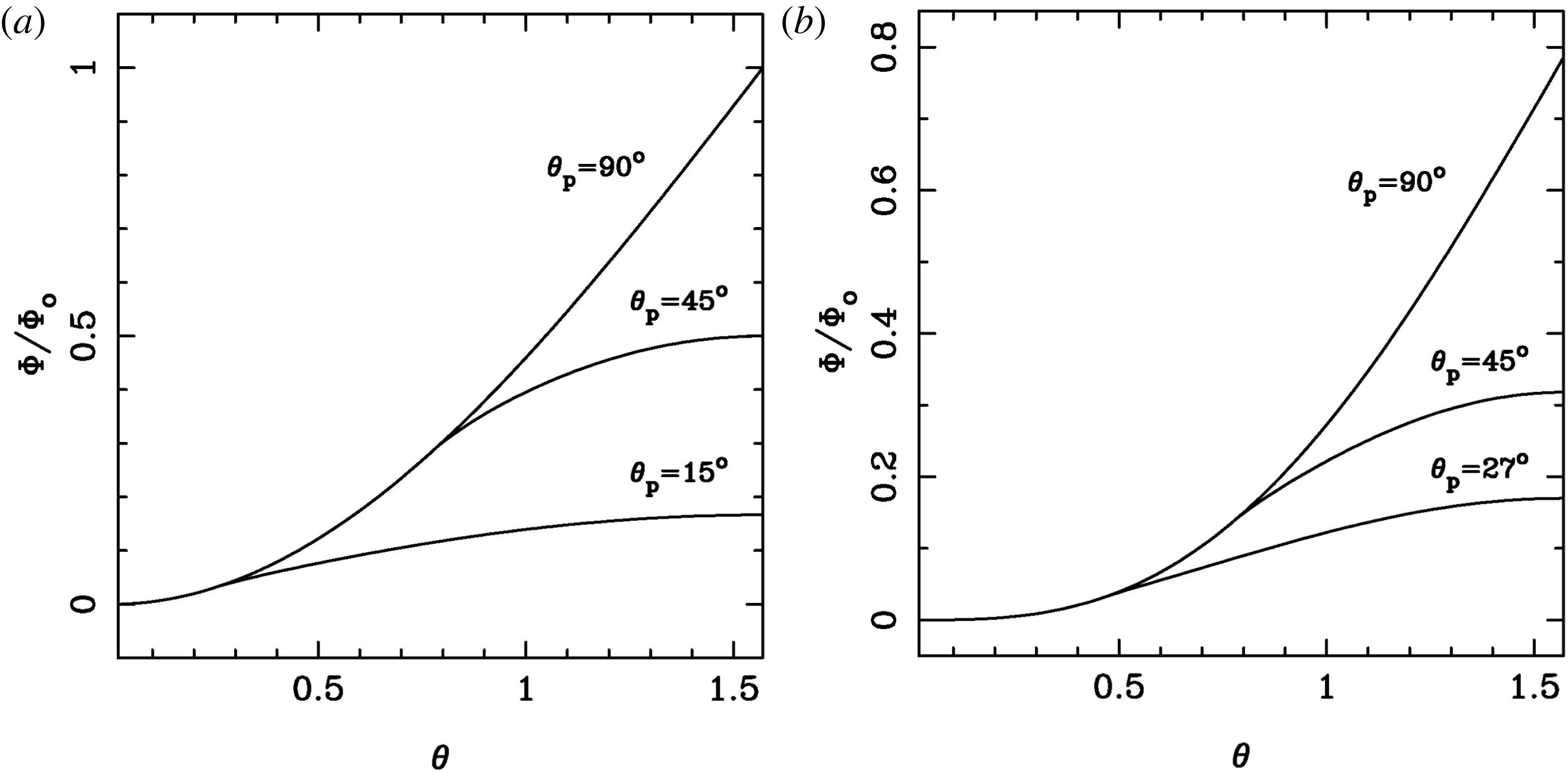
Figure 1. Available potential across the winds depending on the size of the polar zone. (a) Shows the results for
 $n=1$
and (b) for
$n=1$
and (b) for
 $n=2$
.
$n=2$
.
2.1 The wind
In the wind, the magnetic field is dominated by the azimuthal component, whose magnitude varies as
 $$\begin{eqnarray}B_{\unicode[STIX]{x1D719}}(r,\unicode[STIX]{x1D703})=B_{\text{lc}}\left(\frac{r_{\text{lc}}}{r}\right)\sin ^{n}\unicode[STIX]{x1D703},\end{eqnarray}$$
where
 $r_{\text{lc}}=c/\unicode[STIX]{x1D6FA}$
is the radius of light cylinder,
$r_{\text{lc}}=c/\unicode[STIX]{x1D6FA}$
is the radius of light cylinder,
 $B_{\text{lc}}$
is the typical value of
$B_{\text{lc}}$
is the typical value of
 $B$
at the light cylinder and
$B$
at the light cylinder and
 $\unicode[STIX]{x1D6FA}$
is the angular velocity of the pulsar. In the monopole model of the pulsar magnetic field
$\unicode[STIX]{x1D6FA}$
is the angular velocity of the pulsar. In the monopole model of the pulsar magnetic field
 $n=1$
but there is no easy way of finding its value in the more realistic dipolar model. Recent numerical simulations suggest that it could be
$n=1$
but there is no easy way of finding its value in the more realistic dipolar model. Recent numerical simulations suggest that it could be
 $n=2$
(Tchekhovskoy, Philippov & Spitkovsky Reference Tchekhovskoy, Philippov and Spitkovsky2016). This magnetic field is unidirectional in the polar region
$n=2$
(Tchekhovskoy, Philippov & Spitkovsky Reference Tchekhovskoy, Philippov and Spitkovsky2016). This magnetic field is unidirectional in the polar region
 $\unicode[STIX]{x1D703}<\unicode[STIX]{x1D703}_{p}$
but in the equatorial region it comes in the form of stripes with opposite magnetic directions. In the monopole model,
$\unicode[STIX]{x1D703}<\unicode[STIX]{x1D703}_{p}$
but in the equatorial region it comes in the form of stripes with opposite magnetic directions. In the monopole model,
 $\unicode[STIX]{x1D703}_{p}=\unicode[STIX]{x03C0}/2-\unicode[STIX]{x1D6FC}$
, where
$\unicode[STIX]{x1D703}_{p}=\unicode[STIX]{x03C0}/2-\unicode[STIX]{x1D6FC}$
, where
 $\unicode[STIX]{x1D6FC}$
is the angle between the magnetic and rotational axes of the pulsar but in the dipolar model the poloidal field lines are not straight and this relation may no longer hold.
$\unicode[STIX]{x1D6FC}$
is the angle between the magnetic and rotational axes of the pulsar but in the dipolar model the poloidal field lines are not straight and this relation may no longer hold.
For
 $r\gg r_{\text{lc}}$
the wind becomes relativistic and radial and its electric field is dominated by the polar component
$r\gg r_{\text{lc}}$
the wind becomes relativistic and radial and its electric field is dominated by the polar component
 $$\begin{eqnarray}E_{\unicode[STIX]{x1D703}}=(v/c)B_{\unicode[STIX]{x1D719}}=B_{\unicode[STIX]{x1D719}}.\end{eqnarray}$$
The corresponding potential drop across the flow in the polar zone is
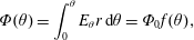 $$\begin{eqnarray}\unicode[STIX]{x1D6F7}(\unicode[STIX]{x1D703})=\int _{0}^{\unicode[STIX]{x1D703}}E_{\unicode[STIX]{x1D703}}r\,\text{d}\unicode[STIX]{x1D703}=\unicode[STIX]{x1D6F7}_{0}f(\unicode[STIX]{x1D703}),\end{eqnarray}$$
where
 $$\begin{eqnarray}\unicode[STIX]{x1D6F7}_{0}=B_{\text{lc}}r_{\text{lc}}\end{eqnarray}$$
and
 $$\begin{eqnarray}f(\unicode[STIX]{x1D703})=\left\{\begin{array}{@{}ll@{}}1-\cos (\unicode[STIX]{x1D703}) & \text{for }n=1\\ 0.5(\unicode[STIX]{x1D703}-0.5\sin 2\unicode[STIX]{x1D703}) & \text{for }n=2.\end{array}\right.\end{eqnarray}$$
In the striped wind zone one has to take into account the alternation of magnetic field direction and use the stripe-averaged magnetic field, which is smaller than that in (2.1) (see Komissarov Reference Komissarov2013). As a result, inside the striped wind zone the potential grows much slower (see figure 1).
The corresponding Poynting vector in the wind is
 $$\begin{eqnarray}\boldsymbol{S}_{P}=\frac{1}{4\unicode[STIX]{x03C0}}E_{\unicode[STIX]{x1D703}}B_{\unicode[STIX]{x1D719}}c=\frac{c}{4\unicode[STIX]{x03C0}}\left(\frac{\unicode[STIX]{x1D6F7}_{0}}{r}\right)^{2}\sin ^{2n}\unicode[STIX]{x1D703},\end{eqnarray}$$
which leads to the total wind power
 $$\begin{eqnarray}L_{w}=a_{n}c\,\unicode[STIX]{x1D6F7}_{0}^{2},\end{eqnarray}$$
where
 $a_{1}=2/3$
and
$a_{1}=2/3$
and
 $a_{2}=8/15$
. Thus one can find
$a_{2}=8/15$
. Thus one can find
 $\unicode[STIX]{x1D6F7}_{0}$
given the measurement of
$\unicode[STIX]{x1D6F7}_{0}$
given the measurement of
 $L_{w}$
as the spindown power of the pulsar. For the Crab pulsar
$L_{w}$
as the spindown power of the pulsar. For the Crab pulsar
 $L_{w}\approx 4\times 10^{38}~\text{erg}~\text{s}^{-1}$
which leads to
$L_{w}\approx 4\times 10^{38}~\text{erg}~\text{s}^{-1}$
which leads to
 $\unicode[STIX]{x1D6F7}_{0}\approx 42~\text{PeV}$
, the corresponding electron Lorentz factor
$\unicode[STIX]{x1D6F7}_{0}\approx 42~\text{PeV}$
, the corresponding electron Lorentz factor
 $$\begin{eqnarray}\unicode[STIX]{x1D6FE}_{\text{max}}\approx 8.2\times 10^{10}\end{eqnarray}$$
and the wind magnetic field
 $$\begin{eqnarray}B_{\unicode[STIX]{x1D719}}\approx 5\times 10^{-2}r_{,\text{ld}}^{-1}\sin ^{n}\unicode[STIX]{x1D703}\,\text{G},\end{eqnarray}$$
where
 $r_{,\text{ld}}$
is the distance measured in light days.
$r_{,\text{ld}}$
is the distance measured in light days.
At the light cylinder, the Goldreich–Julian number density of charged particles
 $$\begin{eqnarray}n_{GJ}=\frac{1}{4\unicode[STIX]{x03C0}e}\,\text{div}\,E\approx \frac{1}{4\unicode[STIX]{x03C0}e}\frac{B_{\text{lc}}}{r_{\text{lc}}}=\frac{1}{4\unicode[STIX]{x03C0}e}\frac{\unicode[STIX]{x1D6F7}_{0}}{r_{\text{lc}}^{2}},\end{eqnarray}$$
whereas the actual density is governed by the pair-production rate
 $n=\unicode[STIX]{x1D706}n_{GJ}$
, where
$n=\unicode[STIX]{x1D706}n_{GJ}$
, where
 $\unicode[STIX]{x1D706}$
is called the multiplicity factor. The corresponding total
$\unicode[STIX]{x1D706}$
is called the multiplicity factor. The corresponding total
 $e_{\pm }$
-particle flux of the wind
$e_{\pm }$
-particle flux of the wind
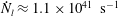
 $$\begin{eqnarray}{\dot{N}}\approx 4\unicode[STIX]{x03C0}r_{\text{lc}}^{2}nc=\frac{\unicode[STIX]{x1D6F7}_{0}c}{e}\approx 8.7\times 10^{37}\unicode[STIX]{x1D706}_{4}~\text{s}^{-1},\end{eqnarray}$$
where
 $\unicode[STIX]{x1D706}_{4}=10^{-4}\unicode[STIX]{x1D706}$
. This corresponds to the particle density in the wind
$\unicode[STIX]{x1D706}_{4}=10^{-4}\unicode[STIX]{x1D706}$
. This corresponds to the particle density in the wind
 $$\begin{eqnarray}n\approx 3.4\times 10^{-5}\unicode[STIX]{x1D706}_{4}r_{,\text{ld}}^{-2}~\text{cm}^{-3}.\end{eqnarray}$$
Along the particle flux tube of a steady-state wind, the particle flux
 $S_{\pm }$
and the total energy flux
$S_{\pm }$
and the total energy flux
 $S_{\text{tot}}=S_{P}+m_{e}c^{2}\unicode[STIX]{x1D6FE}_{w}hS_{\pm }$
, where
$S_{\text{tot}}=S_{P}+m_{e}c^{2}\unicode[STIX]{x1D6FE}_{w}hS_{\pm }$
, where
 $\unicode[STIX]{x1D6FE}_{w}$
is the wind Lorentz factor and
$\unicode[STIX]{x1D6FE}_{w}$
is the wind Lorentz factor and
 $h=w/{\tilde{n}}m_{e}c^{2}$
is the relativistic enthalpy per unit particle rest mass, are conserved. This leads to the integration constant along streamlines
$h=w/{\tilde{n}}m_{e}c^{2}$
is the relativistic enthalpy per unit particle rest mass, are conserved. This leads to the integration constant along streamlines
 $$\begin{eqnarray}\unicode[STIX]{x1D70E}_{M}=\frac{S_{\text{tot}}}{S_{\pm }m_{e}c^{2}}=\unicode[STIX]{x1D6FE}_{w}h(1+\unicode[STIX]{x1D70E}),\end{eqnarray}$$
where
 $\unicode[STIX]{x1D70E}=S_{P}/S_{p}$
is the ratio of the Poynting flux and the particle energy flux
$\unicode[STIX]{x1D70E}=S_{P}/S_{p}$
is the ratio of the Poynting flux and the particle energy flux
 $S_{p}=S_{\pm }m_{e}c^{2}h\unicode[STIX]{x1D6FE}_{w}$
. In the theory of pulsar winds,
$S_{p}=S_{\pm }m_{e}c^{2}h\unicode[STIX]{x1D6FE}_{w}$
. In the theory of pulsar winds,
 $\unicode[STIX]{x1D70E}_{M}$
is known as Michel’s
$\unicode[STIX]{x1D70E}_{M}$
is known as Michel’s
 $\unicode[STIX]{x1D70E}$
(Michel Reference Michel1969) but in the theory of magnetically dominated jets it is simply denoted as
$\unicode[STIX]{x1D70E}$
(Michel Reference Michel1969) but in the theory of magnetically dominated jets it is simply denoted as
 $\unicode[STIX]{x1D707}$
(e.g. Komissarov et al.
Reference Komissarov, Barkov, Vlahakis and Königl2007). Replacing
$\unicode[STIX]{x1D707}$
(e.g. Komissarov et al.
Reference Komissarov, Barkov, Vlahakis and Königl2007). Replacing
 $S_{P}$
and
$S_{P}$
and
 $S_{\pm }$
with their densities,
$S_{\pm }$
with their densities,
 $B_{\unicode[STIX]{x1D719}}^{2}c/4\unicode[STIX]{x03C0}$
and
$B_{\unicode[STIX]{x1D719}}^{2}c/4\unicode[STIX]{x03C0}$
and
 $nc$
respectively, we obtain
$nc$
respectively, we obtain
 $$\begin{eqnarray}\unicode[STIX]{x1D70E}=\frac{B_{\unicode[STIX]{x1D719}}^{2}}{4\unicode[STIX]{x03C0}m_{e}c^{2}hn\unicode[STIX]{x1D6FE}_{w}}=\frac{\tilde{B}_{\unicode[STIX]{x1D719}}^{2}}{4\unicode[STIX]{x03C0}m_{e}c^{2}h{\tilde{n}}},\end{eqnarray}$$
where
 $\tilde{B}$
and
$\tilde{B}$
and
 ${\tilde{n}}$
are measured in the wind frame. Using the parameters at the light cylinder to estimate
${\tilde{n}}$
are measured in the wind frame. Using the parameters at the light cylinder to estimate
 $\unicode[STIX]{x1D70E}_{M}$
, we find
$\unicode[STIX]{x1D70E}_{M}$
, we find
 $$\begin{eqnarray}\unicode[STIX]{x1D70E}_{M}=\frac{\unicode[STIX]{x1D6F7}_{0}e}{m_{e}c^{2}\unicode[STIX]{x1D706}}\approx 8.2\times 10^{6}\unicode[STIX]{x1D706}_{4}^{-1}.\end{eqnarray}$$
For a cold wind
 $h=1$
and hence
$h=1$
and hence
 $$\begin{eqnarray}\unicode[STIX]{x1D6FE}_{w}=\frac{\unicode[STIX]{x1D70E}_{M}}{1+\unicode[STIX]{x1D70E}}.\end{eqnarray}$$
Thus the total conversion of the Poynting flux into the kinetic energy of the bulk motion yields the wind speed
 $$\begin{eqnarray}\unicode[STIX]{x1D6FE}_{w}^{\text{max}}=\unicode[STIX]{x1D70E}_{M}.\end{eqnarray}$$
However in the limit of ideal MHD, reaching this asymptotic value is quite problematic. Indeed, the wind must first become super-fast magnetosonic. At the transonic point
 $$\begin{eqnarray}\unicode[STIX]{x1D6FE}_{w}=\sqrt{\unicode[STIX]{x1D70E}}\end{eqnarray}$$
(e.g. Komissarov Reference Komissarov2012). Combining this result with (2.16) we find that at the fast magnetosonic point
 $$\begin{eqnarray}\unicode[STIX]{x1D6FE}_{w,f}=\unicode[STIX]{x1D70E}_{M}^{1/3}=200\,\unicode[STIX]{x1D706}_{4}^{-1/3}\quad \text{and}\quad \unicode[STIX]{x1D70E}_{f}=4\times 10^{4}\unicode[STIX]{x1D706}_{4}^{-2/3}.\end{eqnarray}$$
Beyond this point the wind becomes causally disconnected, which strongly reduces the efficiency of the ideal collimation–acceleration mechanism (e.g. Beskin, Kuznetsova & Rafikov Reference Beskin, Kuznetsova and Rafikov1998; Komissarov et al.
Reference Komissarov, Vlahakis, Königl and Barkov2009). Thus we do not expect the wind’s Lorentz factor to exceed the value given in (2.20a,b
) by more than a factor of ten. Using the fast magnetosonic Mach number
 $M\approx \unicode[STIX]{x1D6E4}_{w}/\sqrt{\unicode[STIX]{x1D70E}}$
, the wind parameters at the termination shock can be estimated as
$M\approx \unicode[STIX]{x1D6E4}_{w}/\sqrt{\unicode[STIX]{x1D70E}}$
, the wind parameters at the termination shock can be estimated as
 $$\begin{eqnarray}\displaystyle \unicode[STIX]{x1D6FE}_{w,u}=M^{2/3}\unicode[STIX]{x1D70E}_{M}^{1/3}=200\,M^{2/3}\unicode[STIX]{x1D706}_{4}^{-1/3}\quad \text{and}\quad \unicode[STIX]{x1D70E}_{u}=(\unicode[STIX]{x1D70E}_{M}/M)^{2/3}=4\times 10^{4}M^{-2/3}\unicode[STIX]{x1D706}_{4}^{-2/3}. & & \displaystyle \nonumber\\ \displaystyle & & \displaystyle\end{eqnarray}$$
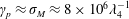
Strictly speaking, these results do not apply to the striped wind zone where the magnetic dissipation of the stripes may come into play and allow some additional acceleration of the flow. Even in the polar zone things can be more complicated if a substantial fraction of the energy is carried away by fast magnetosonic waves emitted into the zone because of the misalignment of the magnetic and rotational axes of the Crab pulsar. Lyubarsky (Reference Lyubarsky2003a
) argues that for
 $\unicode[STIX]{x1D706}\gtrsim 10^{7}$
these waves steepen into shocks and dissipate before reaching the termination shock and the generated heat is quickly converted into the bulk kinetic energy of the wind particles. This process would set an upper limit on the wind magnetisation
$\unicode[STIX]{x1D706}\gtrsim 10^{7}$
these waves steepen into shocks and dissipate before reaching the termination shock and the generated heat is quickly converted into the bulk kinetic energy of the wind particles. This process would set an upper limit on the wind magnetisation
 $\unicode[STIX]{x1D70E}$
at the termination shock equal to the inverse fraction of the energy flux carried by the waves and the Poynting flux of the wind. For example, if the waves contribute only one per cent to the wind energy budget then
$\unicode[STIX]{x1D70E}$
at the termination shock equal to the inverse fraction of the energy flux carried by the waves and the Poynting flux of the wind. For example, if the waves contribute only one per cent to the wind energy budget then
 $\unicode[STIX]{x1D70E}_{u}<100$
. For smaller multiplicity, the waves would dissipate only after crossing the termination shock and the dissipation rate increases sharply in the sub-fast magnetosonic regime (Lyubarsky Reference Lyubarsky2003a
).
$\unicode[STIX]{x1D70E}_{u}<100$
. For smaller multiplicity, the waves would dissipate only after crossing the termination shock and the dissipation rate increases sharply in the sub-fast magnetosonic regime (Lyubarsky Reference Lyubarsky2003a
).
As to the magnetic dissipation in the striped wind zone, its rate can be estimated as follows (Arons Reference Arons2012). In the frame of Earth, the typical thickness of the stripes is
 $l_{s}=cP/2$
, where
$l_{s}=cP/2$
, where
 $P$
is the pulsar period. In the wind frame, it is
$P$
is the pulsar period. In the wind frame, it is
 $l_{s}^{\prime }=\unicode[STIX]{x1D6FE}_{w}cP/2$
and hence the shortest time of stripe dissipation is
$l_{s}^{\prime }=\unicode[STIX]{x1D6FE}_{w}cP/2$
and hence the shortest time of stripe dissipation is
 $t_{s}^{\prime }=\unicode[STIX]{x1D6FE}_{w}P/2$
. In the Earth frame, the time dilation yields
$t_{s}^{\prime }=\unicode[STIX]{x1D6FE}_{w}P/2$
. In the Earth frame, the time dilation yields
 $t_{s}=\unicode[STIX]{x1D6FE}_{w}^{2}P/2$
. Once the dissipation is completed
$t_{s}=\unicode[STIX]{x1D6FE}_{w}^{2}P/2$
. Once the dissipation is completed
 $\unicode[STIX]{x1D6FE}_{w}=\unicode[STIX]{x1D6FE}_{w}^{\text{max}}$
, which yields the distance to this point as
$\unicode[STIX]{x1D6FE}_{w}=\unicode[STIX]{x1D6FE}_{w}^{\text{max}}$
, which yields the distance to this point as
 $$\begin{eqnarray}r_{d}={\textstyle \frac{1}{2}}\unicode[STIX]{x1D70E}_{M}^{2}Pc\approx 1.3\times 10^{7}\unicode[STIX]{x1D706}_{4}^{-2}~\text{light days}.\end{eqnarray}$$
Unless
 $\unicode[STIX]{x1D706}_{4}>300$
this is above the radius of the wind termination shock
$\unicode[STIX]{x1D706}_{4}>300$
this is above the radius of the wind termination shock
 $r_{\text{ts}}\approx 170$
light days (if we identify it with the inner X-ray ring of the Crab Nebula) and the stripes survive all the way up to the termination shock, where
$r_{\text{ts}}\approx 170$
light days (if we identify it with the inner X-ray ring of the Crab Nebula) and the stripes survive all the way up to the termination shock, where
 $\unicode[STIX]{x1D6FE}_{w}\ll \unicode[STIX]{x1D70E}_{M}$
. However, Lyubarsky (Reference Lyubarsky2003b
) has shown that in this case the stripes will dissipate at the termination shock and the post-shock state will be the same as in the case where the stripe dissipation is completed in the wind (see also Sironi & Spitkovsky Reference Sironi and Spitkovsky2012). In both these cases, the magnetisation of the post-shock state is determined by the stripe-averaged magnetic field, which vanishes only in the equatorial plane but is the same as the wind field at the boundary with the polar zone. In the transition between the polar and striped zones the magnetisation parameter drops rapidly from the high value of the polar zone (see (2.20)) to
$\unicode[STIX]{x1D6FE}_{w}\ll \unicode[STIX]{x1D70E}_{M}$
. However, Lyubarsky (Reference Lyubarsky2003b
) has shown that in this case the stripes will dissipate at the termination shock and the post-shock state will be the same as in the case where the stripe dissipation is completed in the wind (see also Sironi & Spitkovsky Reference Sironi and Spitkovsky2012). In both these cases, the magnetisation of the post-shock state is determined by the stripe-averaged magnetic field, which vanishes only in the equatorial plane but is the same as the wind field at the boundary with the polar zone. In the transition between the polar and striped zones the magnetisation parameter drops rapidly from the high value of the polar zone (see (2.20)) to
 $\unicode[STIX]{x1D70E}\approx 1$
and then keeps decreasing with the polar angle, but at a lower rate (Komissarov Reference Komissarov2013).
$\unicode[STIX]{x1D70E}\approx 1$
and then keeps decreasing with the polar angle, but at a lower rate (Komissarov Reference Komissarov2013).
2.2 The nebula
The nebula can be described as a prolate spheroid with the minor axis
 $a\approx 9.5\,\text{ly}$
and the major axis
$a\approx 9.5\,\text{ly}$
and the major axis
 $b\approx 14\,\text{ly}$
(Hester Reference Hester2008). The most spectacular structure of the nebula is its network of thermal filaments. These are associated with the stellar material ejected during the supernova explosion which left behind the Crab pulsar. The non-thermal emission is more diffusive but it also exhibits many features on different length scales. In particular, the radio maps of the nebula show a filamentary structure which is almost identical to network of optical thermal filaments.
$b\approx 14\,\text{ly}$
(Hester Reference Hester2008). The most spectacular structure of the nebula is its network of thermal filaments. These are associated with the stellar material ejected during the supernova explosion which left behind the Crab pulsar. The non-thermal emission is more diffusive but it also exhibits many features on different length scales. In particular, the radio maps of the nebula show a filamentary structure which is almost identical to network of optical thermal filaments.
The X-ray images of the inner nebula reveal an equatorial torus-like structure of the radius of approximately 500 light days and a polar jet of a similar size. Inside the torus, there is an oval structure which looks like a beaded neckless around the pulsar, which is called the ‘X-ray inner ring’. Its radius is
 $r_{ir}\approx 170$
light days. The ring is often interpreted as the termination shock of the pulsar wind. Since the pulsar wind is anisotropic, its termination shock is not spherical and it is most extended in the equatorial plane, where it become transverse and forms the so-called Mach belt (Komissarov & Lyubarsky Reference Komissarov and Lyubarsky2004). On purely geometrical grounds, one is tempted to identify the ring with the Mach belt, but the nature of its emission is not clear. Hester et al. (Reference Hester, Mori, Burrows, Gallagher, Graham, Halverson, Kader, Michel and Scowen2002) state that the beads (knots) of the ring ‘form, brighten, fade, dissipate, move about, and occasionally undergo outbursts, giving rise to expanding clouds of nebulosity’, though no quantitative parameters of this variability are given. Just the naked eye inspection of the Chandra images indicates that their size is approximately one arcsec, which is about the angular resolution of Chandra, corresponding to the linear scale
$r_{ir}\approx 170$
light days. The ring is often interpreted as the termination shock of the pulsar wind. Since the pulsar wind is anisotropic, its termination shock is not spherical and it is most extended in the equatorial plane, where it become transverse and forms the so-called Mach belt (Komissarov & Lyubarsky Reference Komissarov and Lyubarsky2004). On purely geometrical grounds, one is tempted to identify the ring with the Mach belt, but the nature of its emission is not clear. Hester et al. (Reference Hester, Mori, Burrows, Gallagher, Graham, Halverson, Kader, Michel and Scowen2002) state that the beads (knots) of the ring ‘form, brighten, fade, dissipate, move about, and occasionally undergo outbursts, giving rise to expanding clouds of nebulosity’, though no quantitative parameters of this variability are given. Just the naked eye inspection of the Chandra images indicates that their size is approximately one arcsec, which is about the angular resolution of Chandra, corresponding to the linear scale
 ${\approx}10~\text{ld}$
. One cannot exclude that some knots of the ring are even smaller. The ring has no clear identification with features observed in the optical band with HST. However, the HST images reveal a bright compact knot at approximately 0.65 arcsec from the pulsar. This knot is resolved and has the size similar to that of the X-ray knots. The knot is not seen in the radio and X-ray bands (Rudy et al.
Reference Rudy, Horns, DeLuca, Kolodziejczak, Tennant, Yuan, Buehler, Arons, Blandford and Caraveo2015). In addition to these features, there are also fine bright arc-like filaments (‘wisps’) originating in the vicinity of the inner ring and moving away from it with speeds up to
${\approx}10~\text{ld}$
. One cannot exclude that some knots of the ring are even smaller. The ring has no clear identification with features observed in the optical band with HST. However, the HST images reveal a bright compact knot at approximately 0.65 arcsec from the pulsar. This knot is resolved and has the size similar to that of the X-ray knots. The knot is not seen in the radio and X-ray bands (Rudy et al.
Reference Rudy, Horns, DeLuca, Kolodziejczak, Tennant, Yuan, Buehler, Arons, Blandford and Caraveo2015). In addition to these features, there are also fine bright arc-like filaments (‘wisps’) originating in the vicinity of the inner ring and moving away from it with speeds up to
 $0.7\,c.$
These are seen in the radio, optical and X-ray bands, though the wisps seen in different bands are sometimes displaced relative to each other or do not even have a counterpart in the other band (Bietenholz et al.
Reference Bietenholz, Hester, Frail and Bartel2004; Hester Reference Hester2008).
$0.7\,c.$
These are seen in the radio, optical and X-ray bands, though the wisps seen in different bands are sometimes displaced relative to each other or do not even have a counterpart in the other band (Bietenholz et al.
Reference Bietenholz, Hester, Frail and Bartel2004; Hester Reference Hester2008).
The observations of both the synchrotron and inverse-Compton emission of the same population of relativistic leptons allows a more-or-less reliable measurement of the nebula energetics. Using a one-zone model of the nebula, Meyer, Horns & Zechlin (Reference Meyer, Horns and Zechlin2010) arrive at a mean magnetic field strength of
 $B\approx 0.12~\text{mG}$
, with the corresponding magnetic energy density
$B\approx 0.12~\text{mG}$
, with the corresponding magnetic energy density
 $e_{m}\approx 6\times 10^{-10}~\text{erg}~\text{cm}^{-3}$
. The lepton population is split into the low-energy sub-population responsible for the radio synchrotron emission and the high-energy population responsible for the optical through the X-ray to the gamma-ray synchrotron emission. The radio leptons have a hard spectrum,
$e_{m}\approx 6\times 10^{-10}~\text{erg}~\text{cm}^{-3}$
. The lepton population is split into the low-energy sub-population responsible for the radio synchrotron emission and the high-energy population responsible for the optical through the X-ray to the gamma-ray synchrotron emission. The radio leptons have a hard spectrum,
 $$\begin{eqnarray}\text{d}n/\text{d}\unicode[STIX]{x1D6FE}\propto \unicode[STIX]{x1D6FE}^{-p_{r}},\quad p_{r}=1.6,~20<\unicode[STIX]{x1D6FE}<2\times 10^{5}\end{eqnarray}$$
and the optical-X-ray leptons have a soft spectrum,
 $$\begin{eqnarray}\text{d}n/\text{d}\unicode[STIX]{x1D6FE}\propto \unicode[STIX]{x1D6FE}^{-p_{o}},\quad p_{o}=3.2,~4.4\times 10^{5}<\unicode[STIX]{x1D6FE}<3\times 10^{8}.\end{eqnarray}$$
The total energies of the low- and high-energy populations are comparable,
 $E_{l}\approx 3.1\times 10^{48}~\text{erg}$
and
$E_{l}\approx 3.1\times 10^{48}~\text{erg}$
and
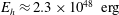 $E_{h}\approx 2.3\times 10^{48}~\text{erg}$
respectively. Given the total volume of the nebula,
$E_{h}\approx 2.3\times 10^{48}~\text{erg}$
respectively. Given the total volume of the nebula,
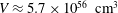 $V\approx 5.7\times 10^{56}~\text{cm}^{3}$
, the corresponding total energy density of the leptons is
$V\approx 5.7\times 10^{56}~\text{cm}^{3}$
, the corresponding total energy density of the leptons is
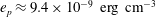 $e_{p}\approx 9.4\times 10^{-9}~\text{erg}~\text{cm}^{-3}$
and the total pressure (leptons
$e_{p}\approx 9.4\times 10^{-9}~\text{erg}~\text{cm}^{-3}$
and the total pressure (leptons
 $+$
magnetic field) is
$+$
magnetic field) is
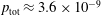 $p_{\text{tot}}\approx 3.6\times 10^{-9}$
. This total pressure can be balanced by the pressure of magnetic field
$p_{\text{tot}}\approx 3.6\times 10^{-9}$
. This total pressure can be balanced by the pressure of magnetic field
 $B=0.3~\text{mG}$
, which is close to the standard equipartition value obtained for the Crab Nebula (Hillas et al.
Reference Hillas, Akerlof, Biller, Buckley, Carter-Lewis, Catanese, Cawley, Fegan, Finley and Gaidos1998).
$B=0.3~\text{mG}$
, which is close to the standard equipartition value obtained for the Crab Nebula (Hillas et al.
Reference Hillas, Akerlof, Biller, Buckley, Carter-Lewis, Catanese, Cawley, Fegan, Finley and Gaidos1998).
The synchrotron cooling of relativistic electrons leads to a break in the particle spectrum at
 $$\begin{eqnarray}\unicode[STIX]{x1D6FE}_{b}=(c_{2}m_{e}c^{2}B_{\bot }^{2}t_{n})^{-1}=1.6\times 10^{6}B_{-4}^{-2}t_{n,3}^{-1},\end{eqnarray}$$
where
 $t_{n,3}$
is the nebula age in units of
$t_{n,3}$
is the nebula age in units of
 $10^{3}\,$
years and
$10^{3}\,$
years and
 $c_{2}=2e^{4}/3m_{e}^{4}c^{7}=0.00237$
in cgs units (Pacholczyk Reference Pacholczyk1970). The corresponding energy of synchrotron photons is
$c_{2}=2e^{4}/3m_{e}^{4}c^{7}=0.00237$
in cgs units (Pacholczyk Reference Pacholczyk1970). The corresponding energy of synchrotron photons is
 $$\begin{eqnarray}{\mathcal{E}}_{\unicode[STIX]{x1D708}}=c_{1}B_{\bot }{\mathcal{E}}^{2}=4.4B_{-4}^{-3}t_{n,3}^{-2}~\text{eV},\end{eqnarray}$$
where
 $c_{1}=3eh/4\unicode[STIX]{x03C0}m_{e}^{3}c^{5}=4.14\times 10^{-8}$
cgs units (Pacholczyk Reference Pacholczyk1970). Thus the spectrum of the optical-X-ray leptons is subject to steepening with the spectral index increasing by unity compared to that of the injection spectrum (Kardashev Reference Kardashev1962), which has to be
$c_{1}=3eh/4\unicode[STIX]{x03C0}m_{e}^{3}c^{5}=4.14\times 10^{-8}$
cgs units (Pacholczyk Reference Pacholczyk1970). Thus the spectrum of the optical-X-ray leptons is subject to steepening with the spectral index increasing by unity compared to that of the injection spectrum (Kardashev Reference Kardashev1962), which has to be
 $a_{i}=2.2$
.
$a_{i}=2.2$
.
Since the nebula has a rich structure on different scales, it is natural to expect strong variations of these parameters from feature to feature. Such variations are observed in the MHD simulations of pulsar wind nebulae (PWN) (Porth et al. Reference Porth, Komissarov and Keppens2013; Olmi et al. Reference Olmi, Del Zanna, Amato, Bucciantini and Mignone2016), with the total pressure exceeding the mean value by up to 5 times at the base of its polar jet and the magnetic field near the termination shock exceeding its mean value by an order of magnitude. Based on these results one may expect the magnetic field in the very inner parts of the Crab Nebula to be as high as one mG.
While it is widely accepted that the high-energy electrons are constantly supplied into the nebula by the pulsar wind, the nature of its radio electrons is still debated. The observed continuity of the synchrotron spectrum at the transition between the populations has been used to argue that the radio electrons are also supplied by the wind (Bucciantini, Arons & Amato Reference Bucciantini, Arons and Amato2011; Arons Reference Arons2012). However, this requires a much more prolific particle-production process in pulsar magnetospheres than the one currently accepted. Given the results by Meyer et al. (Reference Meyer, Horns and Zechlin2010), the high- and low-energy populations contain
 $N_{h}\approx 3.8\times 10^{48}$
and
$N_{h}\approx 3.8\times 10^{48}$
and
 $N_{l}\approx 3.4\times 10^{51}$
leptons respectively. The corresponding number densities are
$N_{l}\approx 3.4\times 10^{51}$
leptons respectively. The corresponding number densities are
 $n_{h}\approx 6.7\times 10^{-9}~\text{cm}^{-3}$
and
$n_{h}\approx 6.7\times 10^{-9}~\text{cm}^{-3}$
and
 $n_{l}\approx 6\times 10^{-6}~\text{cm}^{-3}$
. Given the known age of the nebula
$n_{l}\approx 6\times 10^{-6}~\text{cm}^{-3}$
. Given the known age of the nebula
 $t_{n}=963~\text{yr}$
, the corresponding mean injection rates are
$t_{n}=963~\text{yr}$
, the corresponding mean injection rates are
 ${\dot{N}}_{h}\approx 1.2\times 10^{38}~\text{s}^{-1}$
and
${\dot{N}}_{h}\approx 1.2\times 10^{38}~\text{s}^{-1}$
and
 ${\dot{N}}_{l}\approx 1.1\times 10^{41}~\text{s}^{-1}$
respectively. Comparing these data with (2.11) one finds that if only the high-energy population leptons are injected by the wind then the required multiplicity parameter
${\dot{N}}_{l}\approx 1.1\times 10^{41}~\text{s}^{-1}$
respectively. Comparing these data with (2.11) one finds that if only the high-energy population leptons are injected by the wind then the required multiplicity parameter
 $\unicode[STIX]{x1D706}\approx 10^{4}$
which is consistent with the theory of pair production in pulsar magnetospheres, whereas if the radio leptons are injected as well then
$\unicode[STIX]{x1D706}\approx 10^{4}$
which is consistent with the theory of pair production in pulsar magnetospheres, whereas if the radio leptons are injected as well then
 $\unicode[STIX]{x1D706}\approx 10^{7}$
(Shklovsky Reference Shklovsky1970), which requires a grand revision of this theory (Arons Reference Arons2012). Using (2.12) for the mean number density of particles in the wind one can check the consistency of these estimates of
$\unicode[STIX]{x1D706}\approx 10^{7}$
(Shklovsky Reference Shklovsky1970), which requires a grand revision of this theory (Arons Reference Arons2012). Using (2.12) for the mean number density of particles in the wind one can check the consistency of these estimates of
 $\unicode[STIX]{x1D706}$
with the size of the termination shock. Indeed, at the termination shock the number density of wind particles as measured in the laboratory (Earth’s) frame does not change significantly and should match the observed densities in the nebula. Matching it with
$\unicode[STIX]{x1D706}$
with the size of the termination shock. Indeed, at the termination shock the number density of wind particles as measured in the laboratory (Earth’s) frame does not change significantly and should match the observed densities in the nebula. Matching it with
 $n_{l}$
gives the distance
$n_{l}$
gives the distance
 $$\begin{eqnarray}r\approx 70\,\unicode[STIX]{x1D706}_{7}^{1/2}~\text{ld},\end{eqnarray}$$
whereas matching with
 $n_{h}$
gives
$n_{h}$
gives
 $$\begin{eqnarray}r\approx 70\,\unicode[STIX]{x1D706}_{4}^{1/2}~\text{ld}.\end{eqnarray}$$
These results are consistent with the observations, which give the equatorial radius of the termination shock
 $r_{\text{ts}}\approx 170~\text{ld}$
.
$r_{\text{ts}}\approx 170~\text{ld}$
.
Using
 $\unicode[STIX]{x1D706}=10^{7}$
, we find that upstream of the polar zone of the termination shock
$\unicode[STIX]{x1D706}=10^{7}$
, we find that upstream of the polar zone of the termination shock
 $\unicode[STIX]{x1D6FE}_{u}\approx 20$
and
$\unicode[STIX]{x1D6FE}_{u}\approx 20$
and
 $\unicode[STIX]{x1D70E}_{u}\approx 400$
. This value of
$\unicode[STIX]{x1D70E}_{u}\approx 400$
. This value of
 $\unicode[STIX]{x1D6FE}_{u}$
is approximately the same as the minimum value
$\unicode[STIX]{x1D6FE}_{u}$
is approximately the same as the minimum value
 $\unicode[STIX]{x1D6FE}_{r,\text{min}}$
of Crab’s radio leptons (Meyer et al.
Reference Meyer, Horns and Zechlin2010), which provides some supports the hypothesis that the radio electrons are supplied by the wind. In the absence of stripes one can rule out the shock acceleration mechanism and hence some other acceleration process has to operate downstream of the shock. According to the results derived in Komissarov & Lyutikov (Reference Komissarov and Lyutikov2011), downstream of a highly magnetised shock
$\unicode[STIX]{x1D6FE}_{r,\text{min}}$
of Crab’s radio leptons (Meyer et al.
Reference Meyer, Horns and Zechlin2010), which provides some supports the hypothesis that the radio electrons are supplied by the wind. In the absence of stripes one can rule out the shock acceleration mechanism and hence some other acceleration process has to operate downstream of the shock. According to the results derived in Komissarov & Lyutikov (Reference Komissarov and Lyutikov2011), downstream of a highly magnetised shock
 $$\begin{eqnarray}\unicode[STIX]{x1D6FE}_{d}\approx \sqrt{\unicode[STIX]{x1D70E}_{u}}/\sin \unicode[STIX]{x1D6FF}\quad \text{and}\quad \unicode[STIX]{x1D70E}_{d}\approx \sqrt{\unicode[STIX]{x1D70E}_{u}}\unicode[STIX]{x1D6FE}_{u}\sin \unicode[STIX]{x1D6FF},\end{eqnarray}$$
where
 $\unicode[STIX]{x1D6FF}$
is the angle between the upstream velocity and the shock plane. If the effect of magnetosonic waves is ignored then the upstream parameters can be estimated using (2.20), which yields
$\unicode[STIX]{x1D6FF}$
is the angle between the upstream velocity and the shock plane. If the effect of magnetosonic waves is ignored then the upstream parameters can be estimated using (2.20), which yields
 $\unicode[STIX]{x1D70E}_{u}\approx 400M^{-2/3}\text{ and }\unicode[STIX]{x1D6FE}_{u}\approx 20M^{2/3}$
and hence
$\unicode[STIX]{x1D70E}_{u}\approx 400M^{-2/3}\text{ and }\unicode[STIX]{x1D6FE}_{u}\approx 20M^{2/3}$
and hence
 $$\begin{eqnarray}\unicode[STIX]{x1D6FE}_{d}=20M^{-1/3}/\sin \,\unicode[STIX]{x1D6FF}\quad \text{and}\quad \unicode[STIX]{x1D70E}_{d}=400M^{1/3}\sin \unicode[STIX]{x1D6FF}.\end{eqnarray}$$
We note that
 $\unicode[STIX]{x1D6FE}_{d}$
and
$\unicode[STIX]{x1D6FE}_{d}$
and
 $\unicode[STIX]{x1D70E}_{d}$
depend rather weakly on the wind Mach number, a parameter which we do not know well but do not expect to exceed
$\unicode[STIX]{x1D70E}_{d}$
depend rather weakly on the wind Mach number, a parameter which we do not know well but do not expect to exceed
 $M\approx 10$
by much. The low wind Lorentz factor obtained in this model is consistent with the radio electrons, which also have low Lorentz factors, being supplied by the wind. The high upstream magnetisation rules out particle acceleration at the termination shock and shifts the focus to the processes occurring downstream of the shock instead. The hard spectrum of radio electrons hints at the magnetic reconnection mechanism instead but for
$M\approx 10$
by much. The low wind Lorentz factor obtained in this model is consistent with the radio electrons, which also have low Lorentz factors, being supplied by the wind. The high upstream magnetisation rules out particle acceleration at the termination shock and shifts the focus to the processes occurring downstream of the shock instead. The hard spectrum of radio electrons hints at the magnetic reconnection mechanism instead but for
 $\unicode[STIX]{x1D70E}_{d}>100$
this mechanism yields spectra (Sironi & Spitkovsky Reference Sironi and Spitkovsky2014; Guo et al.
Reference Guo, Liu, Daughton and Li2015) which are even harder, with
$\unicode[STIX]{x1D70E}_{d}>100$
this mechanism yields spectra (Sironi & Spitkovsky Reference Sironi and Spitkovsky2014; Guo et al.
Reference Guo, Liu, Daughton and Li2015) which are even harder, with
 $p\approx 1$
, than that of the radio electronsFootnote
1
. As we have discussed earlier, for this value of the multiplicity parameter the fast magnetosonic waves produced by the pulsar rotation are expected to dissipate upstream of the termination shock (Lyubarsky Reference Lyubarsky2003a
) and hence to reduce
$p\approx 1$
, than that of the radio electronsFootnote
1
. As we have discussed earlier, for this value of the multiplicity parameter the fast magnetosonic waves produced by the pulsar rotation are expected to dissipate upstream of the termination shock (Lyubarsky Reference Lyubarsky2003a
) and hence to reduce
 $\unicode[STIX]{x1D70E}_{u}$
and hence
$\unicode[STIX]{x1D70E}_{u}$
and hence
 $\unicode[STIX]{x1D70E}_{d}$
, provided they carry a fraction of the total energy flux that exceeds
$\unicode[STIX]{x1D70E}_{d}$
, provided they carry a fraction of the total energy flux that exceeds
 $1/\unicode[STIX]{x1D70E}_{u}$
.
$1/\unicode[STIX]{x1D70E}_{u}$
.
For
 $\unicode[STIX]{x1D706}=10^{7}$
the stripes of the pulsar wind get erased before the termination shock, see (2.21), and hence in the equatorial zone the wind entering the shock should have a unidirectional magnetic field, with the magnetisation
$\unicode[STIX]{x1D706}=10^{7}$
the stripes of the pulsar wind get erased before the termination shock, see (2.21), and hence in the equatorial zone the wind entering the shock should have a unidirectional magnetic field, with the magnetisation
 $\unicode[STIX]{x1D70E}<1$
(Komissarov Reference Komissarov2013) and the Lorentz factor
$\unicode[STIX]{x1D70E}<1$
(Komissarov Reference Komissarov2013) and the Lorentz factor
 $\unicode[STIX]{x1D6FE}_{w}=\unicode[STIX]{x1D70E}_{M}\approx 8\times 10^{3}$
. Because these parameters are very different from those of the polar zone one would expect a different particle acceleration regime (or mechanism) as well, leading to different spectral properties of the accelerated particles. This hints a possibility of explaining the existence of two different non-thermal populations of the Crab Nebula – the radio electrons are supplied via the polar zone whereas the high-energy electrons via the equatorial striped zone (cf. Porth et al.
Reference Porth, Komissarov and Keppens2013; Olmi et al.
Reference Olmi, Del Zanna, Amato and Bucciantini2015). However the details are not clear. For example, according to the PIC simulations of relativistic shocks in a pair plasma, the magnetisation has to be as low as
$\unicode[STIX]{x1D6FE}_{w}=\unicode[STIX]{x1D70E}_{M}\approx 8\times 10^{3}$
. Because these parameters are very different from those of the polar zone one would expect a different particle acceleration regime (or mechanism) as well, leading to different spectral properties of the accelerated particles. This hints a possibility of explaining the existence of two different non-thermal populations of the Crab Nebula – the radio electrons are supplied via the polar zone whereas the high-energy electrons via the equatorial striped zone (cf. Porth et al.
Reference Porth, Komissarov and Keppens2013; Olmi et al.
Reference Olmi, Del Zanna, Amato and Bucciantini2015). However the details are not clear. For example, according to the PIC simulations of relativistic shocks in a pair plasma, the magnetisation has to be as low as
 $\unicode[STIX]{x1D70E}=10^{-3}$
for the traditional Fermi mechanism to operate. Such a low magnetisation is expected only in a very narrow equatorial part of the equatorial zone, with the half-opening angle approximately one degree for the magnetic inclination angle
$\unicode[STIX]{x1D70E}=10^{-3}$
for the traditional Fermi mechanism to operate. Such a low magnetisation is expected only in a very narrow equatorial part of the equatorial zone, with the half-opening angle approximately one degree for the magnetic inclination angle
 $\unicode[STIX]{x1D6FC}=45^{\circ }$
(Komissarov Reference Komissarov2013). For the rest of it, the shock is expected only to thermalise the wind particles leading to a Maxwellian-like spectrum with
$\unicode[STIX]{x1D6FC}=45^{\circ }$
(Komissarov Reference Komissarov2013). For the rest of it, the shock is expected only to thermalise the wind particles leading to a Maxwellian-like spectrum with
 $\unicode[STIX]{x1D6FE}_{t}\approx \unicode[STIX]{x1D6FE}_{w}\approx 8\times 10^{3}$
. This would imply strong emission at wavelengths of 1–10 mm associated with the termination shock, which is not seen (Gomez et al.
Reference Gomez, Krause, Barlow, Swinyard, Owen, Clark, Matsuura, Gomez, Rho and Besel2012). Finally, the very idea that the two non-thermal populations could be supplied via different sections of the pulsar wind with very different physical parameters, and presumably shaped via different acceleration mechanisms, reintroduces the difficulty of explaining the continuity of the spectrum of the nebula emission. Moreover, if the radio electrons are supplied via the polar zone then the polar zone should carry about a thousand times more particles than the striped wind zone, which is very hard to explain.
$\unicode[STIX]{x1D6FE}_{t}\approx \unicode[STIX]{x1D6FE}_{w}\approx 8\times 10^{3}$
. This would imply strong emission at wavelengths of 1–10 mm associated with the termination shock, which is not seen (Gomez et al.
Reference Gomez, Krause, Barlow, Swinyard, Owen, Clark, Matsuura, Gomez, Rho and Besel2012). Finally, the very idea that the two non-thermal populations could be supplied via different sections of the pulsar wind with very different physical parameters, and presumably shaped via different acceleration mechanisms, reintroduces the difficulty of explaining the continuity of the spectrum of the nebula emission. Moreover, if the radio electrons are supplied via the polar zone then the polar zone should carry about a thousand times more particles than the striped wind zone, which is very hard to explain.
For the more traditional multiplicity
 $\unicode[STIX]{x1D706}=10^{4}$
the radio electrons cannot be supplied by the wind and must have a different origin. For example, the observed filamentary structure of the synchrotron radio emission suggests that it may be closely related to the supernova ejecta shocked by the pulsar wind (Komissarov Reference Komissarov2013). However the hard spectral index of the radio emission disfavours the diffusive shock acceleration mechanism. As to the termination shock, (2.20) shows that in the polar zone the wind parameters upstream of the shock are
$\unicode[STIX]{x1D706}=10^{4}$
the radio electrons cannot be supplied by the wind and must have a different origin. For example, the observed filamentary structure of the synchrotron radio emission suggests that it may be closely related to the supernova ejecta shocked by the pulsar wind (Komissarov Reference Komissarov2013). However the hard spectral index of the radio emission disfavours the diffusive shock acceleration mechanism. As to the termination shock, (2.20) shows that in the polar zone the wind parameters upstream of the shock are
 $\unicode[STIX]{x1D6FE}_{u}\approx 10^{3}M^{2/3}$
and
$\unicode[STIX]{x1D6FE}_{u}\approx 10^{3}M^{2/3}$
and
 $\unicode[STIX]{x1D70E}_{u}\approx 10^{4}M^{-2/3}$
whereas (2.28) shows that downstream of it
$\unicode[STIX]{x1D70E}_{u}\approx 10^{4}M^{-2/3}$
whereas (2.28) shows that downstream of it
 $$\begin{eqnarray}\unicode[STIX]{x1D6FE}_{d}\approx 10^{3}M^{-1/3}/\sin \unicode[STIX]{x1D6FF}\quad \text{and}\quad \unicode[STIX]{x1D70E}_{d}\approx 10^{4}M^{1/3}\sin \unicode[STIX]{x1D6FF}.\end{eqnarray}$$
These parameters are even more extreme that for
 $\unicode[STIX]{x1D706}=10^{7}$
. Moreover, in this case the fast magnetosonic waves cannot dissipate upstream of the termination shock and hence cannot significantly reduce the wind’s
$\unicode[STIX]{x1D706}=10^{7}$
. Moreover, in this case the fast magnetosonic waves cannot dissipate upstream of the termination shock and hence cannot significantly reduce the wind’s
 $\unicode[STIX]{x1D70E}$
.
$\unicode[STIX]{x1D70E}$
.
As to the striped wind zone, (2.21) tells us that in this case the stripes survive all the way to the termination shock. As they dissipate at the shock, the spectrum of energised particles depends on the value of the parameter
 $$\begin{eqnarray}\unicode[STIX]{x1D701}=4\unicode[STIX]{x03C0}\unicode[STIX]{x1D706}\frac{r_{\text{lc}}}{r_{\text{ts}}}\end{eqnarray}$$
(Sironi & Spitkovsky Reference Sironi and Spitkovsky2011). For
 $\unicode[STIX]{x1D701}<10$
it is a relativistic Maxwellian-like spectrum whereas a broad power-law spectrum is produced only for
$\unicode[STIX]{x1D701}<10$
it is a relativistic Maxwellian-like spectrum whereas a broad power-law spectrum is produced only for
 $\unicode[STIX]{x1D701}>100$
. For the Crab pulsar
$\unicode[STIX]{x1D701}>100$
. For the Crab pulsar
 $r_{\text{lc}}\approx 6\times 10^{-8}\,$
ld and
$r_{\text{lc}}\approx 6\times 10^{-8}\,$
ld and
 $r_{\text{ts}}\approx 170\,$
ld so
$r_{\text{ts}}\approx 170\,$
ld so
 $$\begin{eqnarray}\unicode[STIX]{x1D701}\approx 4\times 10^{-4}\unicode[STIX]{x1D706}_{4}.\end{eqnarray}$$
Thus we expect a Maxwellian-like spectrum peaking at
 $\unicode[STIX]{x1D6FE}_{p}\approx \unicode[STIX]{x1D70E}_{M}\approx 8\times 10^{6}\unicode[STIX]{x1D706}_{4}^{-1}$
. The corresponding synchrotron frequency
$\unicode[STIX]{x1D6FE}_{p}\approx \unicode[STIX]{x1D70E}_{M}\approx 8\times 10^{6}\unicode[STIX]{x1D706}_{4}^{-1}$
. The corresponding synchrotron frequency
 $$\begin{eqnarray}\unicode[STIX]{x1D708}=5\times 10^{16}B_{-3}\unicode[STIX]{x1D706}_{4}^{-2}~\text{Hz}.\end{eqnarray}$$
The inner knot of the Crab Nebula is currently associated with the emission of shocked striped wind (Lyutikov et al.
Reference Lyutikov, Komissarov and Porth2016). The knot is seen only in the optical and near IR bands. Given that the theory predicts a Doppler shift of the knot emission by a factor of a few towards higher energies, this requires
 $\unicode[STIX]{x1D706}\approx 10^{5}$
, which seems quite realistic. More observational data on the knot emission are required to clarify the nature of its emission.
$\unicode[STIX]{x1D706}\approx 10^{5}$
, which seems quite realistic. More observational data on the knot emission are required to clarify the nature of its emission.
The above analysis shows a glaring conflict between the observations and the current understanding of relativistic magnetised shocks as particle accelerators. Either the current shock theory based on PIC simulations is completely wrong or the observed spectrum is shaped by other processes. These could be a second-order Fermi mechanism of particle acceleration by plasma turbulence or magnetic reconnection, both occurring inside the nebula.
3 Papers I and II: particle acceleration in explosive reconnection events
In papers I and II we have discussed intensively the properties of particle acceleration during the X-point collapse (paper I), during the development of the 2-D ABC instability and during the merger of flux tube with zero total current (paper II). Here we briefly summarise the main results. Overall, the papers investigate particle acceleration during flux merger events in a relativistic highly magnetised plasma.
In paper I we studied the initial stages of the current sheet formation – the X-point collapse, and generalised a classic plasma physics work by Syrovatskii (Reference Syrovatskii1981) to the highly magnetised regime. Starting from a slightly unbalanced X-point configuration, large-scale magnetic stresses lead to explosive formation of a current sheet. During the X-point collapse particles are accelerated by charge-starved electric fields, which can reach (and even exceed) values of the local magnetic field. The explosive stage of reconnection produces non-thermal power-law tails with slopes that depend on the average magnetisation
 $\unicode[STIX]{x1D70E}$
. The X-point collapse stage is followed by magnetic island merger that dissipates a large fraction of the initial magnetic energy in a regime of forced magnetic reconnection, further accelerating the particles, but proceeds at a slower reconnection rate.
$\unicode[STIX]{x1D70E}$
. The X-point collapse stage is followed by magnetic island merger that dissipates a large fraction of the initial magnetic energy in a regime of forced magnetic reconnection, further accelerating the particles, but proceeds at a slower reconnection rate.
In paper II we addressed evolution on somewhat larger scales, conducting a number of numerical simulations of merging flux tubes with zero poloidal current. The key difference between this case and the X-point collapse is that two zero current flux tubes immersed either in external magnetic field or external plasma represent a stable configuration – two barely touching flux tubes, basically, do not evolve – there are no large-scale stresses that force the islands to merge. When the two flux tubes are pushed together, the initial evolution depends on the transient character of the initial conditions.
In all the different configurations that we investigated the evolution proceeded according to a similar scenario: initially, perturbation lead to the reconnection of outer field lines and the formation of a common envelope. This initial stage of the merger proceeds very slowly, driven by resistive effects. With time the envelope grew in size and a common magnetic envelope develops around the cores. The dynamics changes when the two cores of the flux tube (which carry parallel currents) come into contact. Starting at this moment, the evolution of the two merging cores resembles the X-point collapse: the cores start to merge explosively and, similarly, are later balanced by the forming current sheet. Particle acceleration proceeds here in a qualitatively similar way as in the case of pure X-point collapse.
The different set-ups allow us to concentrate on somewhat different aspects of particle acceleration. In all the cases that we investigated the efficient particle acceleration always occurs in the region with
 $E\geqslant B$
– by the charge-starved electric fields. This stage is best probed with the X-point collapse simulations, paper I. In the case of ABC structures and flux tube mergers particles are accelerated most efficiently during the initial explosive stage; during that stage not much of magnetic energy is dissipated. In the case of a 2-D ABC system, this initial stage of rapid acceleration is followed by a forced reconnection stage; at this stage particles are further accelerated to higher energies, but the rate of acceleration is low. In the case of the colliding/merging zero current flux tubes, the fast dynamic stage is preceded by the slow resistive stage, when the outer field lines form an overlaying shroud that pushes the parallel current-carrying cores together. When these parallel current-carrying cores come in contact the evolution proceeds similarly to the unstable ABC case. We stress that the fastest particle acceleration occurs at the beginning of the dynamical stage of the merger (right away in the X-point collapse simulations, in the initial stage of the instability of the ABC configuration, after the slow resistive evolution in case of colliding/merging flux tubes).
$E\geqslant B$
– by the charge-starved electric fields. This stage is best probed with the X-point collapse simulations, paper I. In the case of ABC structures and flux tube mergers particles are accelerated most efficiently during the initial explosive stage; during that stage not much of magnetic energy is dissipated. In the case of a 2-D ABC system, this initial stage of rapid acceleration is followed by a forced reconnection stage; at this stage particles are further accelerated to higher energies, but the rate of acceleration is low. In the case of the colliding/merging zero current flux tubes, the fast dynamic stage is preceded by the slow resistive stage, when the outer field lines form an overlaying shroud that pushes the parallel current-carrying cores together. When these parallel current-carrying cores come in contact the evolution proceeds similarly to the unstable ABC case. We stress that the fastest particle acceleration occurs at the beginning of the dynamical stage of the merger (right away in the X-point collapse simulations, in the initial stage of the instability of the ABC configuration, after the slow resistive evolution in case of colliding/merging flux tubes).
4 Gamma-ray flares as reconnection events
4.1 Peak energy
The fact that the peak energy of the Crab flares is located about the radiation-reaction limit for the synchrotron mechanism suggests that the observed radiation is produced in this regime, whereby the energy gains due to the acceleration mechanism are balanced by the energy losses via the synchrotron radiation. Accelerated particles are confined to the current sheet where the magnetic field is weaker compared to the reconnecting magnetic field
 $B$
outside. Moreover only the component of magnetic field perpendicular to the particle momentum contributes to the synchrotron energy loss. Denoting this component as
$B$
outside. Moreover only the component of magnetic field perpendicular to the particle momentum contributes to the synchrotron energy loss. Denoting this component as
 $B_{a,\bot }=\unicode[STIX]{x1D705}B$
, where
$B_{a,\bot }=\unicode[STIX]{x1D705}B$
, where
 $0<\unicode[STIX]{x1D705}<1$
, we can write the energy loss rate by a particle of energy
$0<\unicode[STIX]{x1D705}<1$
, we can write the energy loss rate by a particle of energy
 ${\mathcal{E}}$
as
${\mathcal{E}}$
as
 $$\begin{eqnarray}\frac{\text{d}{\mathcal{E}}}{\text{d}t}=-c_{2}B_{a,\bot }^{2}{\mathcal{E}}^{2},\end{eqnarray}$$
where
 $c_{2}=2e^{4}/3m_{e}^{4}c^{7}=0.00237$
in cgs units. The energy gain is via the electrostatic acceleration by the reconnection electric field
$c_{2}=2e^{4}/3m_{e}^{4}c^{7}=0.00237$
in cgs units. The energy gain is via the electrostatic acceleration by the reconnection electric field
 $$\begin{eqnarray}\frac{\text{d}{\mathcal{E}}}{\text{d}t}=eE_{a}c,\end{eqnarray}$$
where
 $E_{a}=\unicode[STIX]{x1D702}B$
is the electric field and
$E_{a}=\unicode[STIX]{x1D702}B$
is the electric field and
 $0<\unicode[STIX]{x1D702}<1$
is the reconnection rate. The balance between the two yields the electron energy
$0<\unicode[STIX]{x1D702}<1$
is the reconnection rate. The balance between the two yields the electron energy
 $$\begin{eqnarray}{\mathcal{E}}_{\text{max}}=\frac{1}{\unicode[STIX]{x1D705}}\left(\frac{\unicode[STIX]{x1D702}ec}{c_{2}B}\right)=1.53\frac{\unicode[STIX]{x1D702}^{1/2}}{\unicode[STIX]{x1D705}}B_{-3}^{-1/2}~\text{PeV},\end{eqnarray}$$
where
 $B_{-3}$
is the magnetic field in mG. The corresponding Lorentz factor of flare-producing leptons is
$B_{-3}$
is the magnetic field in mG. The corresponding Lorentz factor of flare-producing leptons is
 $$\begin{eqnarray}\unicode[STIX]{x1D6FE}=3\times 10^{9}\frac{\unicode[STIX]{x1D702}^{1/2}}{\unicode[STIX]{x1D705}}B_{-3}^{-1/2}.\end{eqnarray}$$
This is approximately 30 times smaller than the maximal possible Lorentz factor based on the electric potential drop across the pulsar wind given by (2.8), thus supporting the possibility of electrostatic acceleration. Using (2.3)–(2.5) one can estimate the minimum size of the polar wind zone delivering the required potential drop. For
 $\unicode[STIX]{x1D6FE}=3\times 10^{9}$
this is
$\unicode[STIX]{x1D6FE}=3\times 10^{9}$
this is
 $$\begin{eqnarray}\unicode[STIX]{x1D703}_{p}^{\text{min}}=\left\{\begin{array}{@{}ll@{}}15^{\circ } & \text{for }n=1;\\ 27^{\circ } & \text{for }n=2.\end{array}\right.\end{eqnarray}$$
These are reasonably small compared to
 $\unicode[STIX]{x1D703}_{p}\approx 45^{\circ }$
estimated for the Crab pulsar (Harding et al.
Reference Harding, Stern, Dyks and Frackowiak2008; Lyutikov et al.
Reference Lyutikov, Komissarov and Porth2016).
$\unicode[STIX]{x1D703}_{p}\approx 45^{\circ }$
estimated for the Crab pulsar (Harding et al.
Reference Harding, Stern, Dyks and Frackowiak2008; Lyutikov et al.
Reference Lyutikov, Komissarov and Porth2016).
The energy of synchrotron photons emitted by the particle of energy
 ${\mathcal{E}}$
in the magnetic field
${\mathcal{E}}$
in the magnetic field
 $B$
is
$B$
is
 $$\begin{eqnarray}{\mathcal{E}}_{\unicode[STIX]{x1D708}}=c_{1}B_{\bot }{\mathcal{E}}^{2},\end{eqnarray}$$
where
 $c_{1}=3eh/4\unicode[STIX]{x03C0}m_{e}^{3}c^{5}=4.14\times 10^{-8}$
cgs units (Pacholczyk Reference Pacholczyk1970). It is observed in the simulations (Cerutti et al.
Reference Cerutti, Werner, Uzdensky and Begelman2013) that the highest-energy photons are emitted when the accelerated particle is ejected from the current layer into the reconnecting magnetic field. With this understanding of
$c_{1}=3eh/4\unicode[STIX]{x03C0}m_{e}^{3}c^{5}=4.14\times 10^{-8}$
cgs units (Pacholczyk Reference Pacholczyk1970). It is observed in the simulations (Cerutti et al.
Reference Cerutti, Werner, Uzdensky and Begelman2013) that the highest-energy photons are emitted when the accelerated particle is ejected from the current layer into the reconnecting magnetic field. With this understanding of
 $B$
in (4.6) we find the maximum energy of photons emitted from the reconnection region as
$B$
in (4.6) we find the maximum energy of photons emitted from the reconnection region as
 $$\begin{eqnarray}{\mathcal{E}}_{\unicode[STIX]{x1D708},\text{max}}=\frac{c_{1}}{c_{2}}\frac{\unicode[STIX]{x1D702}}{\unicode[STIX]{x1D705}^{2}}ec=158\left(\frac{\unicode[STIX]{x1D702}}{\unicode[STIX]{x1D705}^{2}}\right)~\text{MeV}.\end{eqnarray}$$
In papers I and II we show that for the reconnection driven by macroscopic stresses in a highly magnetised plasma, the reconnection speed approaches the speed of light and hence
 $\unicode[STIX]{x1D702}\rightarrow 1$
(papers I and II). Thus
$\unicode[STIX]{x1D702}\rightarrow 1$
(papers I and II). Thus
 $\unicode[STIX]{x1D705}\simeq 0.5$
is sufficient to explain the peak photon energy of Crab flares.
$\unicode[STIX]{x1D705}\simeq 0.5$
is sufficient to explain the peak photon energy of Crab flares.
The acceleration time required to reach
 ${\mathcal{E}}_{\text{max}}$
is
${\mathcal{E}}_{\text{max}}$
is
 $$\begin{eqnarray}t_{\text{acc}}=\frac{{\mathcal{E}}_{\text{max}}}{\unicode[STIX]{x1D702}eBc}=2\frac{1}{\unicode[STIX]{x1D705}\unicode[STIX]{x1D702}^{1/2}}B_{-3}^{-3/2}~\text{days},\end{eqnarray}$$
whereas the gyration period of an electron with this energy in the reconnecting magnetic field is
 $$\begin{eqnarray}t_{g}=2\unicode[STIX]{x03C0}\unicode[STIX]{x1D702}t_{\text{acc}}.\end{eqnarray}$$
The corresponding gyration radius is
 $$\begin{eqnarray}r_{g}=\unicode[STIX]{x1D702}ct_{\text{acc}}.\end{eqnarray}$$
4.2 Size and energetics of the flaring site
The acceleration time sets the lower limit on the size of the ‘accelerator’ (the current layer)
 $$\begin{eqnarray}l_{\text{min}}=ct_{\text{acc}}=2\frac{1}{\unicode[STIX]{x1D705}\unicode[STIX]{x1D702}^{1/2}}B_{-3}^{-3/2}~\text{light days}.\end{eqnarray}$$
Interestingly, this differs from the gyration radius of the electrons with energy
 ${\mathcal{E}}_{\text{max}}$
only by the factor
${\mathcal{E}}_{\text{max}}$
only by the factor
 $1/\unicode[STIX]{x1D702}$
. Assuming that the reconnection region is not moving with relativistic speed, the actual size of the active region should fall within the bounds
$1/\unicode[STIX]{x1D702}$
. Assuming that the reconnection region is not moving with relativistic speed, the actual size of the active region should fall within the bounds
 $$\begin{eqnarray}l_{\text{min}}<l<ct_{f},\end{eqnarray}$$
where
 $t_{f}$
is the flare duration. Because
$t_{f}$
is the flare duration. Because
 $t_{f}$
is of the order of a few days, the last two equations imply that the reconnecting magnetic field cannot be significantly below
$t_{f}$
is of the order of a few days, the last two equations imply that the reconnecting magnetic field cannot be significantly below
 $1\,$
mG. As we discussed in § 2.2,
$1\,$
mG. As we discussed in § 2.2,
 $B\approx 1~\text{mG}$
is too high for most of the nebula but it is not unreasonable for the very inner part of the Crab Nebula. In fact, direct application of (2.9) shows that the wind magnetic field has such a strength at the distance
$B\approx 1~\text{mG}$
is too high for most of the nebula but it is not unreasonable for the very inner part of the Crab Nebula. In fact, direct application of (2.9) shows that the wind magnetic field has such a strength at the distance
 $r=50\sin ^{n}\unicode[STIX]{x1D703}$
light days, which is significantly smaller compared to the equatorial radius of the termination shock. For
$r=50\sin ^{n}\unicode[STIX]{x1D703}$
light days, which is significantly smaller compared to the equatorial radius of the termination shock. For
 $B=1~\text{mG}$
the gyration of electrons with energy
$B=1~\text{mG}$
the gyration of electrons with energy
 ${\mathcal{E}}_{\text{max}}$
is of the order of the size of the active region. This implies that they cannot be trapped by the magnetic islands (ropes) as their size is much smaller compared to the length of the current sheet.
${\mathcal{E}}_{\text{max}}$
is of the order of the size of the active region. This implies that they cannot be trapped by the magnetic islands (ropes) as their size is much smaller compared to the length of the current sheet.
The total magnetic energy of the flare region is
 $$\begin{eqnarray}E_{m}=7\times 10^{38}B_{-3}^{2}l_{\text{ld}}^{3}~\text{erg},\end{eqnarray}$$
where
 $l_{\text{ld}}$
is the size of the region in light days. If a fraction
$l_{\text{ld}}$
is the size of the region in light days. If a fraction
 $\unicode[STIX]{x1D716}_{m}$
of this energy is converted into emission with
$\unicode[STIX]{x1D716}_{m}$
of this energy is converted into emission with
 ${\mathcal{E}}_{\unicode[STIX]{x1D708}}>100~\text{MeV}$
then the corresponding mean luminosity of the flare is
${\mathcal{E}}_{\unicode[STIX]{x1D708}}>100~\text{MeV}$
then the corresponding mean luminosity of the flare is
 $$\begin{eqnarray}L=8\times 10^{33}\unicode[STIX]{x1D716}_{m}B_{-3}^{2}\,l_{\text{ld}}^{3}\,t_{f,d}^{-1}~\text{erg}~\text{s}^{-1},\end{eqnarray}$$
where
 $t_{f,d}$
is the flare duration in days. Since
$t_{f,d}$
is the flare duration in days. Since
 $l$
cannot exceed
$l$
cannot exceed
 $ct_{f}$
, the highest possible luminosity is
$ct_{f}$
, the highest possible luminosity is
 $$\begin{eqnarray}L_{\text{max}}=8\times 10^{33}\unicode[STIX]{x1D716}_{m}B_{-3}^{2}\,t_{f,d}^{2}~\text{erg}~\text{s}^{-1}.\end{eqnarray}$$
For the April 2011 flare
 $t_{f,d}=4$
and hence
$t_{f,d}=4$
and hence
 $L_{\text{max}}=1.5\times 10^{35}\unicode[STIX]{x1D716}_{m}B_{-3}^{2}~\text{erg}~\text{s}^{-1}$
whereas the observed isotropic luminosity above 100 MeV is
$L_{\text{max}}=1.5\times 10^{35}\unicode[STIX]{x1D716}_{m}B_{-3}^{2}~\text{erg}~\text{s}^{-1}$
whereas the observed isotropic luminosity above 100 MeV is
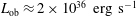 $L_{\text{ob}}\approx 2\times 10^{36}~\text{erg}~\text{s}^{-1}$
. This suggests that either the magnetic field is a few times over 1 mG or the flare emission is beamed with the beaming factor
$L_{\text{ob}}\approx 2\times 10^{36}~\text{erg}~\text{s}^{-1}$
. This suggests that either the magnetic field is a few times over 1 mG or the flare emission is beamed with the beaming factor
 $f_{b}=\unicode[STIX]{x0394}\unicode[STIX]{x1D6FA}/4\unicode[STIX]{x03C0}\approx L_{\text{max}}/L_{\text{ob}}\lesssim 0.08\unicode[STIX]{x1D716}_{m}B_{-3}^{2}$
, where
$f_{b}=\unicode[STIX]{x0394}\unicode[STIX]{x1D6FA}/4\unicode[STIX]{x03C0}\approx L_{\text{max}}/L_{\text{ob}}\lesssim 0.08\unicode[STIX]{x1D716}_{m}B_{-3}^{2}$
, where
 $\unicode[STIX]{x0394}\unicode[STIX]{x1D6FA}$
is the beam solid angle. The angular distribution of particles accelerated in the current layers is not isotropic and the degree of anisotropy increases with the particle energy (Cerutti et al.
Reference Cerutti, Werner, Uzdensky and Begelman2012b
, Paper I). This kinetic beaming of accelerated particles is reflected in the anisotropy of their synchrotron emission with the beaming factor near the peak of the emission spectrum
$\unicode[STIX]{x0394}\unicode[STIX]{x1D6FA}$
is the beam solid angle. The angular distribution of particles accelerated in the current layers is not isotropic and the degree of anisotropy increases with the particle energy (Cerutti et al.
Reference Cerutti, Werner, Uzdensky and Begelman2012b
, Paper I). This kinetic beaming of accelerated particles is reflected in the anisotropy of their synchrotron emission with the beaming factor near the peak of the emission spectrum
 $f_{b}\approx 0.1$
, which is consistent with our estimate for the April 2011 flare.
$f_{b}\approx 0.1$
, which is consistent with our estimate for the April 2011 flare.
If the reconnecting region is moving relative to the Earth with a relativistic speed then its observed emission can also be beamed due to the Doppler effect. The half-opening angle of the Doppler beam corresponding to the solid angle
 $\unicode[STIX]{x0394}\unicode[STIX]{x1D6FA}/4\unicode[STIX]{x03C0}\approx 0.08$
is
$\unicode[STIX]{x0394}\unicode[STIX]{x1D6FA}/4\unicode[STIX]{x03C0}\approx 0.08$
is
 $\unicode[STIX]{x1D703}_{d}\approx 35^{\circ }$
, which corresponds to the bulk speed
$\unicode[STIX]{x1D703}_{d}\approx 35^{\circ }$
, which corresponds to the bulk speed
 $v\approx 0.5c$
. Such speeds are typical for the inner Crab Nebula. Even higher speeds are expected in the polar region at the base of the Crab’s jet on theoretical grounds (see § 2.2).
$v\approx 0.5c$
. Such speeds are typical for the inner Crab Nebula. Even higher speeds are expected in the polar region at the base of the Crab’s jet on theoretical grounds (see § 2.2).
4.3 Spectrum of emitting particles
One can estimate the number of gamma-ray-emitting leptons in the flaring region as
 $N_{\unicode[STIX]{x1D6FE}}\approx Lt_{\text{cool}}/{\mathcal{E}}_{\text{max}}$
. Assuming that the cooling time
$N_{\unicode[STIX]{x1D6FE}}\approx Lt_{\text{cool}}/{\mathcal{E}}_{\text{max}}$
. Assuming that the cooling time
 $t_{\text{cool}}=t_{\text{acc}}$
and using (4.8) and (4.15), we find
$t_{\text{cool}}=t_{\text{acc}}$
and using (4.8) and (4.15), we find
 $$\begin{eqnarray}N_{\unicode[STIX]{x1D6FE}}\approx 5.6\times 10^{35}\frac{\unicode[STIX]{x1D716}_{m}}{\unicode[STIX]{x1D702}}B_{-3}t_{f,d}^{2}.\end{eqnarray}$$
(Comparing this with the pair-production rate of the pulsar, equation (2.11), one can see that it takes a fraction of a second to generate the particles producing the flares.) The corresponding volume density
 $$\begin{eqnarray}n_{\unicode[STIX]{x1D6FE}}\approx 3\times 10^{-11}B_{-3}t_{f,d}^{-1}~\text{cm}^{-3}\end{eqnarray}$$
is significantly smaller than the number densities of both the high-energy and low-energy lepton populations in the nebula. This shows that only a tiny fraction of particles in the flaring region are accelerated to the energies required to produce its gamma-ray emission.
Most studies of particle acceleration in magnetic reconnection come up with a single power law for the non-thermal particles. Our study also indicates a clear possibility of two populations of accelerated particles: a less energetic population with a softer spectrum which is made out of particles trapped inside the magnetic islands (ropes) and a more energetic population with a very hard spectrum made out of particles which are free inside the current sheet (paper I). Only the latter one would produce the flare emission. When the synchrotron radiation losses are taken into account one can also expect a pile up of particles near the radiation-reaction limit (Clausen-Brown & Lyutikov Reference Clausen-Brown and Lyutikov2012). Keeping these caveats in mind we will use here a simple model which involves a single power-law spectrum truncated at both ends of the energy domain
 $$\begin{eqnarray}\frac{\text{d}n}{\text{d}\unicode[STIX]{x1D6FE}}=A\unicode[STIX]{x1D6FE}^{-p},\quad \unicode[STIX]{x1D6FE}_{\text{min}}\leqslant \unicode[STIX]{x1D6FE}\leqslant \unicode[STIX]{x1D6FE}_{\text{max}}.\end{eqnarray}$$
The corresponding spectrum of the synchrotron photons is also a power law
 $\text{d}n_{\unicode[STIX]{x1D708}}/\text{d}{\mathcal{E}}\propto {\mathcal{E}}^{-a}$
, where
$\text{d}n_{\unicode[STIX]{x1D708}}/\text{d}{\mathcal{E}}\propto {\mathcal{E}}^{-a}$
, where
 $$\begin{eqnarray}p=1+2(a-1).\end{eqnarray}$$
For the April 2011 flare this gives
 $p=1.54\pm 0.24$
. Since
$p=1.54\pm 0.24$
. Since
 $1<p<2$
one can estimate the total number density as
$1<p<2$
one can estimate the total number density as
 $$\begin{eqnarray}n_{\text{tot}}=A\unicode[STIX]{x1D6FE}_{\text{min}}^{1-p}/(p-1)\end{eqnarray}$$
and the density of gamma-ray-emitting leptons as
 $$\begin{eqnarray}n_{\unicode[STIX]{x1D6FE}}=A\unicode[STIX]{x1D6FE}_{\text{max}}^{1-p}.\end{eqnarray}$$
Combining the two, we find
 $$\begin{eqnarray}\frac{n_{\text{tot}}}{n_{\unicode[STIX]{x1D6FE}}}=\frac{1}{p-1}\left(\frac{\unicode[STIX]{x1D6FE}_{\text{max}}}{\unicode[STIX]{x1D6FE}_{\text{min}}}\right)^{p-1}.\end{eqnarray}$$
The corresponding mean Lorentz factor
 $$\begin{eqnarray}\langle \unicode[STIX]{x1D6FE}\rangle =\unicode[STIX]{x1D6FE}_{\text{max}}\frac{p-1}{2-p}\left(\frac{\unicode[STIX]{x1D6FE}_{\text{max}}}{\unicode[STIX]{x1D6FE}_{\text{min}}}\right)^{1-p},\end{eqnarray}$$
has to be equal to
 $\unicode[STIX]{x1D70E}_{M}$
. From the last two equations we find the simple equation
$\unicode[STIX]{x1D70E}_{M}$
. From the last two equations we find the simple equation
 $$\begin{eqnarray}\unicode[STIX]{x1D6FE}_{\text{max}}=(2-p)\unicode[STIX]{x1D70E}_{M}\left(\frac{n_{\text{tot}}}{n_{\unicode[STIX]{x1D6FE}}}\right),\end{eqnarray}$$
which allows us to check the self-consistency of the model. Substituting the expressions for
 $\unicode[STIX]{x1D70E}_{M}$
from (2.15),
$\unicode[STIX]{x1D70E}_{M}$
from (2.15),
 $n_{\unicode[STIX]{x1D6FE}}$
from (4.17), using
$n_{\unicode[STIX]{x1D6FE}}$
from (4.17), using
 $t_{d}=4$
and assuming that the wind supplies only the high-energy leptons (
$t_{d}=4$
and assuming that the wind supplies only the high-energy leptons (
 $n_{\text{tot}}\approx n_{h}$
), we obtain
$n_{\text{tot}}\approx n_{h}$
), we obtain
 $$\begin{eqnarray}\unicode[STIX]{x1D6FE}_{\text{max}}\approx 3.4\times 10^{9}\unicode[STIX]{x1D706}_{4}^{-1}B_{-3}^{-1},\end{eqnarray}$$
which is very close to the estimate (4.4). If the wind supplies the radio electrons as well then
 $n_{\text{tot}}\approx n_{l}$
and
$n_{\text{tot}}\approx n_{l}$
and
 $$\begin{eqnarray}\unicode[STIX]{x1D6FE}_{\text{max}}\approx 3\times 10^{9}\unicode[STIX]{x1D706}_{7}^{-1}B_{-3}^{-1},\end{eqnarray}$$
which is an equally good result. Next we can use (4.22) to find
 $$\begin{eqnarray}\unicode[STIX]{x1D6FE}_{\text{min}}=\unicode[STIX]{x1D6FE}_{\text{max}}\left(\frac{n_{\unicode[STIX]{x1D6FE}}}{n_{\text{tot}}}\frac{1}{p-1}\right)^{1/(p-1)}.\end{eqnarray}$$
In this equation
 $\unicode[STIX]{x1D6FE}_{\text{min}}$
is very sensitive to the power index. In the model where the wind supplies only the high-energy population, we find that for
$\unicode[STIX]{x1D6FE}_{\text{min}}$
is very sensitive to the power index. In the model where the wind supplies only the high-energy population, we find that for
 $p=1.54\pm 0.24$
 $\unicode[STIX]{x1D6FE}_{\text{min}}$
varies in the range
$\unicode[STIX]{x1D6FE}_{\text{min}}$
varies in the range
 $\unicode[STIX]{x1D6FE}_{\text{min}}\in (3\times 10^{3},5\times 10^{6})$
with the median value of
$\unicode[STIX]{x1D6FE}_{\text{min}}\in (3\times 10^{3},5\times 10^{6})$
with the median value of
 $5\times 10^{5}$
, corresponding to the optical electrons. If the wind supplies the radio electrons as well then
$5\times 10^{5}$
, corresponding to the optical electrons. If the wind supplies the radio electrons as well then
 $\unicode[STIX]{x1D6FE}_{\text{min}}\in (4\times 10^{-7},750)$
with a median value of
$\unicode[STIX]{x1D6FE}_{\text{min}}\in (4\times 10^{-7},750)$
with a median value of
 $1.6$
, showing that only
$1.6$
, showing that only
 $p\leqslant 1.54$
are acceptable. Interestingly, the observed spectral index of the radio electrons
$p\leqslant 1.54$
are acceptable. Interestingly, the observed spectral index of the radio electrons
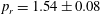 $p_{r}=1.54\pm 0.08$
(Kovalenko, Pynzar’ & Udal’Tsov Reference Kovalenko, Pynzar’ and Udal’Tsov1994; Bietenholz et al.
Reference Bietenholz, Kassim, Frail, Perley, Erickson and Hajian1997) is very close to that of the gamma-ray flare electrons.
$p_{r}=1.54\pm 0.08$
(Kovalenko, Pynzar’ & Udal’Tsov Reference Kovalenko, Pynzar’ and Udal’Tsov1994; Bietenholz et al.
Reference Bietenholz, Kassim, Frail, Perley, Erickson and Hajian1997) is very close to that of the gamma-ray flare electrons.
4.4 Plasma parameters
The observed spectra of flares provide some information on the plasma magnetisation of the flaring region. According to the PIC simulations (Sironi & Spitkovsky Reference Sironi and Spitkovsky2014; Guo et al.
Reference Guo, Liu, Daughton and Li2015, Papers I and II,),
 $p\approx 1.5$
requires the plasma magnetisation
$p\approx 1.5$
requires the plasma magnetisation
 $\unicode[STIX]{x1D70E}$
to be of the order of a few tens, with
$\unicode[STIX]{x1D70E}$
to be of the order of a few tens, with
 $\unicode[STIX]{x1D70E}>100$
leading to very hard spectra with
$\unicode[STIX]{x1D70E}>100$
leading to very hard spectra with
 $p\rightarrow 1$
and
$p\rightarrow 1$
and
 $\unicode[STIX]{x1D70E}<10$
to soft spectra
$\unicode[STIX]{x1D70E}<10$
to soft spectra
 $p>2$
.
$p>2$
.
Another important parameter is the electron skin depth
 $\unicode[STIX]{x1D6FF}_{s}=c/\unicode[STIX]{x1D714}_{p}$
, where
$\unicode[STIX]{x1D6FF}_{s}=c/\unicode[STIX]{x1D714}_{p}$
, where
 $\unicode[STIX]{x1D714}_{p}^{2}=4\unicode[STIX]{x03C0}e^{2}n/(m_{e}\unicode[STIX]{x1D6FE}_{t})$
is the plasma frequency and
$\unicode[STIX]{x1D714}_{p}^{2}=4\unicode[STIX]{x03C0}e^{2}n/(m_{e}\unicode[STIX]{x1D6FE}_{t})$
is the plasma frequency and
 $\unicode[STIX]{x1D6FE}_{t}$
is the mean Lorentz factor of particles in the reconnection inflow. Assuming that the flare occurs in a plasma whose bulk motion Lorentz factor is of the order of unity but
$\unicode[STIX]{x1D6FE}_{t}$
is the mean Lorentz factor of particles in the reconnection inflow. Assuming that the flare occurs in a plasma whose bulk motion Lorentz factor is of the order of unity but
 $\unicode[STIX]{x1D70E}\gg 1$
, one can estimate
$\unicode[STIX]{x1D70E}\gg 1$
, one can estimate
 $\unicode[STIX]{x1D6FE}_{t}\approx \unicode[STIX]{x1D70E}_{M}/\unicode[STIX]{x1D70E}$
and hence
$\unicode[STIX]{x1D6FE}_{t}\approx \unicode[STIX]{x1D70E}_{M}/\unicode[STIX]{x1D70E}$
and hence
 $$\begin{eqnarray}\unicode[STIX]{x1D714}_{p}^{2}\approx \frac{4\unicode[STIX]{x03C0}e^{2}}{m_{e}}\frac{n}{\unicode[STIX]{x1D70E}_{M}}\unicode[STIX]{x1D70E},\end{eqnarray}$$
which is sensitive to what we assume about the origin of radio electrons. If they are not supplied by the wind then
 $n\approx n_{h}$
and
$n\approx n_{h}$
and
 $$\begin{eqnarray}\unicode[STIX]{x1D6FF}_{s}\approx \frac{7\times 10^{-3}}{\sqrt{\unicode[STIX]{x1D706}_{4}\unicode[STIX]{x1D70E}}}~\text{ld}\end{eqnarray}$$
and if they are then
 $n\approx n_{l}$
and
$n\approx n_{l}$
and
 $$\begin{eqnarray}\unicode[STIX]{x1D6FF}_{s}\approx \frac{8\times 10^{-6}}{\sqrt{\unicode[STIX]{x1D706}_{7}\unicode[STIX]{x1D70E}}}~\text{ld}.\end{eqnarray}$$
Thus, the size of the flaring region
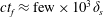 $ct_{f}\approx \text{few}\times 10^{3}\unicode[STIX]{x1D6FF}_{s}$
and
$ct_{f}\approx \text{few}\times 10^{3}\unicode[STIX]{x1D6FF}_{s}$
and
 $\text{few}\times 10^{6}\unicode[STIX]{x1D6FF}_{s}$
respectively. The corresponding plasma gyration radius
$\text{few}\times 10^{6}\unicode[STIX]{x1D6FF}_{s}$
respectively. The corresponding plasma gyration radius
 $$\begin{eqnarray}r_{g}=\frac{m_{e}c^{2}\unicode[STIX]{x1D6FE}_{t}}{eB}=\unicode[STIX]{x1D6FF}_{s}/\unicode[STIX]{x1D70E}\end{eqnarray}$$
is even smaller than
 $\unicode[STIX]{x1D6FF}_{s}$
. Thus, the Crab flares undoubtedly involve macroscopic scales.
$\unicode[STIX]{x1D6FF}_{s}$
. Thus, the Crab flares undoubtedly involve macroscopic scales.
As the wind flow is brought to a virtual halt in the flaring site,
 $\unicode[STIX]{x1D6FE}_{w}\approx 1$
and
$\unicode[STIX]{x1D6FE}_{w}\approx 1$
and
 $$\begin{eqnarray}\unicode[STIX]{x1D70E}_{M}=h\unicode[STIX]{x1D70E}=\frac{B^{2}}{4\unicode[STIX]{x03C0}m_{e}c^{2}n}.\end{eqnarray}$$
This yields an independent estimate of the reconnecting magnetic field strength, namely
 $$\begin{eqnarray}B=(4\unicode[STIX]{x03C0}m_{e}c^{2}n\unicode[STIX]{x1D70E}_{M})^{1/2}\approx 0.7~\text{mG}.\end{eqnarray}$$
The result is not sensitive to the assumption on the origin of the radio electrons (If the radio electrons are supplied by the wind then we should use
 $n=n_{l}$
and
$n=n_{l}$
and
 $\unicode[STIX]{x1D706}=10^{7}$
and if they are not then
$\unicode[STIX]{x1D706}=10^{7}$
and if they are not then
 $n=n_{h}$
and
$n=n_{h}$
and
 $\unicode[STIX]{x1D706}=10^{7}$
, which leaves
$\unicode[STIX]{x1D706}=10^{7}$
, which leaves
 $n\unicode[STIX]{x1D70E}_{M}$
unchanged.). This is quite close to the lower limit on the magnetic field strength obtained in § 4.2.
$n\unicode[STIX]{x1D70E}_{M}$
unchanged.). This is quite close to the lower limit on the magnetic field strength obtained in § 4.2.
4.5 Potential–luminosity relationship and the Alfvén current
There is an important, yet somewhat subtle, relationship between the parameters of the flares that serve as a confirmation of the basic principles of our approach, as we discuss next. In addition to particle acceleration, the reconnecting electric field also drives (a charge-separated) current. This induced current creates its own magnetic field; particle gyration in the induced magnetic field can inhibit the beam propagation. These considerations place an upper limit on the total charger-separated current, known as the Alfvén current. The relativistic Alfvén current (Alfvén Reference Alfvén1939; Lawson Reference Lawson1973) is
 $$\begin{eqnarray}I_{A}=\unicode[STIX]{x1D6FE}\frac{m_{e}c^{3}}{e}.\end{eqnarray}$$
In the present model of Crab flares, the reconnection events result in a population of gamma-ray-emitting particles. Those particles create electric current, which in turn creates its own magnetic field. For the consistency of the model it is required that the Larmor radius of the particles in their own magnetic field is sufficiently large. Next, using the total flare luminosity and the estimates of the energy of emitting particles we can verify that the current carried by the flare-emitting particles does not violate the Alfvén limit.
Qualitatively, the electromagnetic power of relativistic outflows can be estimated as (Blandford & Znajek Reference Blandford and Znajek1977; Blandford Reference Blandford, Gilfanov, Sunyeav and Churazov2002)
 $$\begin{eqnarray}L_{EM}\approx V^{2}/{\mathcal{R}},\end{eqnarray}$$
where
 $V$
is a typical values of the electric potential produced by the central engine and
$V$
is a typical values of the electric potential produced by the central engine and
 ${\mathcal{R}}\approx 1/c$
is the impedance of free space. In case of Crab flares, the available potential,
${\mathcal{R}}\approx 1/c$
is the impedance of free space. In case of Crab flares, the available potential,
 $$\begin{eqnarray}V\sim \sqrt{L/c}\approx 1.7\times 10^{15}~\text{V},\end{eqnarray}$$
corresponds to
 $\unicode[STIX]{x1D6FE}\approx 3.4\times 10^{9}$
– very close to the estimate (4.4).
$\unicode[STIX]{x1D6FE}\approx 3.4\times 10^{9}$
– very close to the estimate (4.4).
Similarly, the electric current associated with flares
 $$\begin{eqnarray}I\approx \sqrt{Lc}\approx 5\times 10^{22}~\text{cgs units}=1.7\times 10^{13}~\text{A}\end{eqnarray}$$
is similar to the Alfvén current (4.34) for the required Lorentz factor (4.4):
 $$\begin{eqnarray}I_{A}=1.7\times 10^{23},~\text{cgs units}=6\times 10^{13}~\text{A}.\end{eqnarray}$$
This is important: the Lorentz factor that we derived from radiation modelling (from the peak energy and duration of flares) nearly coincides with the expected Lorentz factor of particles derived from the assumption that the radiated power is similar to the intrinsic electromagnetic power of the flares. In a related ‘coincidence’, the current required to produce a given luminosity nearly coincides with the corresponding Alfvén current, calculated using the Lorentz factor of the emitting particles.
These coincidences, in our view, are not accidental: they imply that flares are produced by charge-separated flow. This is indeed expected in the acceleration models based on DC-type acceleration. This is also consistent with our PIC simulation that shows the effects of kinetic beaming – a highly anisotropic distribution of the highest-energy particles.
5 The likely site
5.1 Magnetisation in different parts of the nebula
After reviewing the theory and observations of the Crab Nebula and the analysis of its gamma-ray flares as magnetic reconnection events, we are now ready to identify the locations in the nebula where this flaring emission may be coming from. In fact, it is quite clear that for most of the Crab Nebula the physical conditions are not favourable for the flares. Firstly, the mean magnetic field of the nebula is approximately an order of magnitude below the minimum strength of one mG required for the accelerated particles to reach the radiation-reaction limit on the typical time scale of the flares (see § 4.2). Secondly, the mean magnetic energy density is approximately an order of magnitude below that of the synchrotron electrons, which implies that the mean magnetisation parameter can be at most
 $\unicode[STIX]{x1D70E}\approx 0.1$
. For such a low magnetisation, the reconnection rate can be at most
$\unicode[STIX]{x1D70E}\approx 0.1$
. For such a low magnetisation, the reconnection rate can be at most
 $\unicode[STIX]{x1D702}\approx 0.1$
. This not only increases the required acceleration time even further, see (4.11), but also reduces the photon energy in radiation-reaction limit by an order of magnitude (see (4.7)). Finally, for
$\unicode[STIX]{x1D702}\approx 0.1$
. This not only increases the required acceleration time even further, see (4.11), but also reduces the photon energy in radiation-reaction limit by an order of magnitude (see (4.7)). Finally, for
 $\unicode[STIX]{x1D70E}<1$
the spectrum of accelerated particles becomes too soft, with the power index
$\unicode[STIX]{x1D70E}<1$
the spectrum of accelerated particles becomes too soft, with the power index
 $p>4$
(Sironi & Spitkovsky Reference Sironi and Spitkovsky2014; Guo et al.
Reference Guo, Liu, Daughton and Li2015), whereas the observations suggest a hard power-law spectrum with
$p>4$
(Sironi & Spitkovsky Reference Sironi and Spitkovsky2014; Guo et al.
Reference Guo, Liu, Daughton and Li2015), whereas the observations suggest a hard power-law spectrum with
 $p\approx 1.5$
(Buehler et al.
Reference Buehler, Scargle, Blandford, Baldini, Baring, Belfiore, Charles, Chiang, D’Ammando and Dermer2012) or even a monoenergetic spectrum (Striani et al.
Reference Striani, Tavani, Vittorini, Donnarumma, Giuliani, Pucella, Argan, Bulgarelli, Colafrancesco and Cardillo2013). If the flares do occur inside the nebula then these must be rather special cites with much stronger magnetic field and much higher magnetisation. In principle, strong shocks may amplify the magnetic field. The RMHD computer simulations of PWN show that secondary shocks are indeed emitted by the highly variable termination shock of the pulsar wind but they are rather weak (Camus et al.
Reference Camus, Komissarov, Bucciantini and Hughes2009; Porth et al.
Reference Porth, Komissarov and Keppens2013). Moreover, RMHD shocks cannot change the plasma magnetisation from
$p\approx 1.5$
(Buehler et al.
Reference Buehler, Scargle, Blandford, Baldini, Baring, Belfiore, Charles, Chiang, D’Ammando and Dermer2012) or even a monoenergetic spectrum (Striani et al.
Reference Striani, Tavani, Vittorini, Donnarumma, Giuliani, Pucella, Argan, Bulgarelli, Colafrancesco and Cardillo2013). If the flares do occur inside the nebula then these must be rather special cites with much stronger magnetic field and much higher magnetisation. In principle, strong shocks may amplify the magnetic field. The RMHD computer simulations of PWN show that secondary shocks are indeed emitted by the highly variable termination shock of the pulsar wind but they are rather weak (Camus et al.
Reference Camus, Komissarov, Bucciantini and Hughes2009; Porth et al.
Reference Porth, Komissarov and Keppens2013). Moreover, RMHD shocks cannot change the plasma magnetisation from
 $\unicode[STIX]{x1D70E}\ll 1$
to
$\unicode[STIX]{x1D70E}\ll 1$
to
 $\unicode[STIX]{x1D70E}\gg 1$
. The simulations also indicate that near the termination shock the physical conditions can be more extreme so we now turn our attention to the very vicinity of the shock.
$\unicode[STIX]{x1D70E}\gg 1$
. The simulations also indicate that near the termination shock the physical conditions can be more extreme so we now turn our attention to the very vicinity of the shock.
In the analysis of the termination shock and physical parameters of the plasma injected by the pulsar wind into the nebula one should differentiate between its polar section, terminating the unstriped polar part of the wind, and its equatorial section, terminating the striped equatorial part of the wind. As Lyutikov et al. (Reference Lyutikov, Komissarov and Porth2016) discuss, the modelling of the inner knot of the Crab Nebula requires that the equatorial flow is weakly magnetised. Thus, the physical conditions downstream of the striped section are still not quite suitable for a flaring site. Indeed, whether the radio electrons are supplied by the wind or not, the downstream magnetisation is very low, with
 $\unicode[STIX]{x1D70E}\ll 1$
. If the radio electrons are supplied by the wind, then its stripes dissipate and its magnetisation drops to very low levels before the termination shock. If the radio electrons are not supplied by the wind then the stripes dissipate at the termination shock. As we have discussed, for the parameters of the Crab wind this dissipation leads only to plasma heating (§ 2.2) and the downstream magnetisation is too low to make gamma-ray flares via reconnection of the residual magnetic field. The observations of the inner knot of the Crab Nebula, which is best explained as a Doppler-boosted emission of the shocked striped wind (Lyutikov et al.
Reference Lyutikov, Komissarov and Porth2016), agree with this verdict – its optical and IR emission does not correlate with the gamma-ray flares (Rudy et al.
Reference Rudy, Horns, DeLuca, Kolodziejczak, Tennant, Yuan, Buehler, Arons, Blandford and Caraveo2015).
$\unicode[STIX]{x1D70E}\ll 1$
. If the radio electrons are supplied by the wind, then its stripes dissipate and its magnetisation drops to very low levels before the termination shock. If the radio electrons are not supplied by the wind then the stripes dissipate at the termination shock. As we have discussed, for the parameters of the Crab wind this dissipation leads only to plasma heating (§ 2.2) and the downstream magnetisation is too low to make gamma-ray flares via reconnection of the residual magnetic field. The observations of the inner knot of the Crab Nebula, which is best explained as a Doppler-boosted emission of the shocked striped wind (Lyutikov et al.
Reference Lyutikov, Komissarov and Porth2016), agree with this verdict – its optical and IR emission does not correlate with the gamma-ray flares (Rudy et al.
Reference Rudy, Horns, DeLuca, Kolodziejczak, Tennant, Yuan, Buehler, Arons, Blandford and Caraveo2015).
What remains is the poleward zone of the nebula which is filled with the plasma supplied by the unstriped polar section of the pulsar wind. As we discussed in § 2.2, here the magnetisation can be very high
 $\unicode[STIX]{x1D70E}\gg 1$
leading to the reconnection rate
$\unicode[STIX]{x1D70E}\gg 1$
leading to the reconnection rate
 $\unicode[STIX]{x1D702}\approx 1$
and very hard spectra of accelerated particles. Moreover, the polar region is over-pressured compared to the rest of the nebula due the hoop stress of the azimuthal magnetic field freshly supplied by the pulsar wind and hence its total pressure and the magnetic field strength can be much higher. Early axisymmetric numerical solutions, based on models of weakly magnetised pulsar winds, exhibited such magnetic pinch all the way to the outer edge of the nebula (e.g. Camus et al.
Reference Camus, Komissarov, Bucciantini and Hughes2009). However in the recent 3-D RMHD simulations of PWN (Porth et al.
Reference Porth, Komissarov and Keppens2013; Olmi et al.
Reference Olmi, Del Zanna, Amato, Bucciantini and Mignone2016) such a strong compression is found only at the base of the polar jet, on a scale not exceeding the equatorial size of the termination shock. Further out the z-pinch appears to be destroyed by instabilities.
$\unicode[STIX]{x1D702}\approx 1$
and very hard spectra of accelerated particles. Moreover, the polar region is over-pressured compared to the rest of the nebula due the hoop stress of the azimuthal magnetic field freshly supplied by the pulsar wind and hence its total pressure and the magnetic field strength can be much higher. Early axisymmetric numerical solutions, based on models of weakly magnetised pulsar winds, exhibited such magnetic pinch all the way to the outer edge of the nebula (e.g. Camus et al.
Reference Camus, Komissarov, Bucciantini and Hughes2009). However in the recent 3-D RMHD simulations of PWN (Porth et al.
Reference Porth, Komissarov and Keppens2013; Olmi et al.
Reference Olmi, Del Zanna, Amato, Bucciantini and Mignone2016) such a strong compression is found only at the base of the polar jet, on a scale not exceeding the equatorial size of the termination shock. Further out the z-pinch appears to be destroyed by instabilities.
The total potential drop across the polar zone of the Crab’s pulsar wind is also sufficiently high to accommodate particle acceleration up to
 $\unicode[STIX]{x1D6FE}\approx 3\times 10^{9}$
, required by the observations, unless the opening angle of the polar zone is below
$\unicode[STIX]{x1D6FE}\approx 3\times 10^{9}$
, required by the observations, unless the opening angle of the polar zone is below
 $15^{\circ }$
for
$15^{\circ }$
for
 $n=1$
and
$n=1$
and
 $27^{\circ }$
for
$27^{\circ }$
for
 $n=2$
.
$n=2$
.
As the polar angle decreases below the value of
 $\unicode[STIX]{x1D703}_{p}$
separating the striped and polar wind zones, the termination shock shrinks dramatically in reaction to the much higher magnetisation of the polar zone (Lyubarsky Reference Lyubarsky2012; Lyutikov et al.
Reference Lyutikov, Komissarov and Porth2016). Using the asymptotic solution given in Lyutikov et al. (Reference Lyutikov, Komissarov and Porth2016), we find that in the polar zone the shock’s spherical radius
$\unicode[STIX]{x1D703}_{p}$
separating the striped and polar wind zones, the termination shock shrinks dramatically in reaction to the much higher magnetisation of the polar zone (Lyubarsky Reference Lyubarsky2012; Lyutikov et al.
Reference Lyutikov, Komissarov and Porth2016). Using the asymptotic solution given in Lyutikov et al. (Reference Lyutikov, Komissarov and Porth2016), we find that in the polar zone the shock’s spherical radius
 $$\begin{eqnarray}R(\unicode[STIX]{x1D703})\simeq \frac{R_{o}}{\sqrt{2\unicode[STIX]{x1D70E}_{u}}}\left\{\begin{array}{@{}ll@{}}\unicode[STIX]{x1D703}^{2}/2 & \text{for }n=1\\ \unicode[STIX]{x1D703}^{3}/3 & \text{for }n=2,\end{array}\right.\end{eqnarray}$$
where
 $R_{o}=(S_{p}/4\unicode[STIX]{x03C0}cp_{p})^{1/2}$
and
$R_{o}=(S_{p}/4\unicode[STIX]{x03C0}cp_{p})^{1/2}$
and
 $p_{p}$
is the total pressure of the polar region. The equatorial radius of the termination shock can be estimated as
$p_{p}$
is the total pressure of the polar region. The equatorial radius of the termination shock can be estimated as
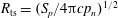 $R_{\text{ts}}=(S_{p}/4\unicode[STIX]{x03C0}cp_{n})^{1/2}$
, where
$R_{\text{ts}}=(S_{p}/4\unicode[STIX]{x03C0}cp_{n})^{1/2}$
, where
 $p_{n}$
is the mean total pressure of the nebula. Given
$p_{n}$
is the mean total pressure of the nebula. Given
 $p_{p}\approx 10p_{n}$
and
$p_{p}\approx 10p_{n}$
and
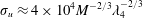 $\unicode[STIX]{x1D70E}_{u}\approx 4\times 10^{4}M^{-2/3}\unicode[STIX]{x1D706}_{4}^{-2/3}$
predicted by the ideal MHD model of the pulsar wing, the maximum distance of the termination shock from the pulsar can be well below one light day. Even if fast magnetosonic waves are responsible for a non-negligible fraction of the initial energy transport in the polar zone and dissipate before reaching the termination shock, the distance is still rather short. A two per cent fraction leads to
$\unicode[STIX]{x1D70E}_{u}\approx 4\times 10^{4}M^{-2/3}\unicode[STIX]{x1D706}_{4}^{-2/3}$
predicted by the ideal MHD model of the pulsar wing, the maximum distance of the termination shock from the pulsar can be well below one light day. Even if fast magnetosonic waves are responsible for a non-negligible fraction of the initial energy transport in the polar zone and dissipate before reaching the termination shock, the distance is still rather short. A two per cent fraction leads to
 $\unicode[STIX]{x1D70E}_{u}=50$
and
$\unicode[STIX]{x1D70E}_{u}=50$
and
 $R<3~\text{ld}$
. So we may be dealing with a rather compact region here.
$R<3~\text{ld}$
. So we may be dealing with a rather compact region here.
For
 $\unicode[STIX]{x1D70E}_{u}\gg 1$
the shock is weak, the speed of the downstream flow is very close to the speed of light and it is highly magnetised. It has to somehow decelerate further in order to match the slow expansion rate of the nebula. Lyubarsky (Reference Lyubarsky2012) analysed a steady-state axisymmetric model of this polar flow assuming that it is confined by the mean pressure of the nebula, using the approximation of
$\unicode[STIX]{x1D70E}_{u}\gg 1$
the shock is weak, the speed of the downstream flow is very close to the speed of light and it is highly magnetised. It has to somehow decelerate further in order to match the slow expansion rate of the nebula. Lyubarsky (Reference Lyubarsky2012) analysed a steady-state axisymmetric model of this polar flow assuming that it is confined by the mean pressure of the nebula, using the approximation of
 $\unicode[STIX]{x1D703}_{p}\ll 1$
and assuming
$\unicode[STIX]{x1D703}_{p}\ll 1$
and assuming
 $n=1$
. He concluded that the flow converges on the scale
$n=1$
. He concluded that the flow converges on the scale
 $$\begin{eqnarray}R_{c}=\frac{\unicode[STIX]{x03C0}}{\sqrt{6}}\unicode[STIX]{x1D703}_{p}^{2}R_{\text{ts}}\end{eqnarray}$$
and argued that at this point it will be destroyed by instabilities. For
 $\unicode[STIX]{x1D703}_{p}=30^{\circ }$
, equation (5.2) yields
$\unicode[STIX]{x1D703}_{p}=30^{\circ }$
, equation (5.2) yields
 $R_{c}\approx 0.35R_{\text{ts}}$
. Given that the external pressure in the polar region can exceed the mean pressure of the nebula by an order of magnitude,
$R_{c}\approx 0.35R_{\text{ts}}$
. Given that the external pressure in the polar region can exceed the mean pressure of the nebula by an order of magnitude,
 $R_{c}$
can be reduced by a factor of three, leading to
$R_{c}$
can be reduced by a factor of three, leading to
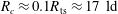 $R_{c}\approx 0.1R_{\text{ts}}\approx 17~\text{ld}$
in the case of the Crab.
$R_{c}\approx 0.1R_{\text{ts}}\approx 17~\text{ld}$
in the case of the Crab.
5.2 Current filamentation
Recent 3-D RMHD simulations of PWN produced by winds with distinctly different polar and equatorial zones (Porth, Komissarov & Keppens Reference Porth, Komissarov and Keppens2014) offer further insight into the dynamics of the polar region. As the mildly relativistic post-shock flow decelerates, it comes into a global causal contact. Once causally connected, the almost purely toroidal magnetic configuration of the nebula flow is liable to current-driven instabilities Begelman (Reference Begelman1998), Mizuno et al. (Reference Mizuno, Lyubarsky, Nishikawa and Hardee2011). As pointed out by Lyubarsky (Reference Lyubarsky2012), in a highly magnetised expanding post-shock flow, the flow lines are in fact focussed to the axis via the magnetic hoop stress which can act as an additional trigger for instability. Thereby the innermost flow reaches the recollimation point first and is expected to experience violent instability and magnetic dissipation. Lyubarsky (Reference Lyubarsky2012) hence argues that the gamma-ray flares originate in the polar region at the base of the observed jet/plume. On the one hand, the simulations of Porth et al. (Reference Porth, Komissarov and Keppens2014) are in agreement with this dynamical picture and show development of modes with azimuthal number
 $m\sim \text{few}$
, that lead to the formation of current filaments at the jet base. On the other hand, for numerical stability, Porth et al. (Reference Porth, Komissarov and Keppens2014) could only study moderate polar magnetisations of
$m\sim \text{few}$
, that lead to the formation of current filaments at the jet base. On the other hand, for numerical stability, Porth et al. (Reference Porth, Komissarov and Keppens2014) could only study moderate polar magnetisations of
 $\unicode[STIX]{x1D70E}\leqslant 3$
which disfavour rapid particle acceleration. Even without this technical limitation, for non-vanishing wind power, the axis itself cannot carry a DC Poynting flux. Because of this, we are interested in flow lines from intermediate latitudes that acquire high
$\unicode[STIX]{x1D70E}\leqslant 3$
which disfavour rapid particle acceleration. Even without this technical limitation, for non-vanishing wind power, the axis itself cannot carry a DC Poynting flux. Because of this, we are interested in flow lines from intermediate latitudes that acquire high
 $\unicode[STIX]{x1D70E}$
due to flow expansion.
$\unicode[STIX]{x1D70E}$
due to flow expansion.
To visualise the current in the simulations, we now cut the domain by spherical surfaces and investigate current magnitude and magnetisation in the
 $\unicode[STIX]{x1D719}\unicode[STIX]{x1D703}$
-plane. In general, the current exhibits a quadrupolar morphology, it is distributed smoothly over the polar regions and returns near the equator. When the test surface crosses over the termination shock, we observe an increased return current due to the shock jump of
$\unicode[STIX]{x1D719}\unicode[STIX]{x1D703}$
-plane. In general, the current exhibits a quadrupolar morphology, it is distributed smoothly over the polar regions and returns near the equator. When the test surface crosses over the termination shock, we observe an increased return current due to the shock jump of
 $B_{\unicode[STIX]{x1D719}}$
. Although the field is predominantly toroidal in the high
$B_{\unicode[STIX]{x1D719}}$
. Although the field is predominantly toroidal in the high
 $\unicode[STIX]{x1D70E}$
downstream region, perturbations from the unstable jet occasionally lead to current filaments and even reversals just downstream of the termination shock.
$\unicode[STIX]{x1D70E}$
downstream region, perturbations from the unstable jet occasionally lead to current filaments and even reversals just downstream of the termination shock.
With increasing distance from the termination shock, the flow becomes more and more turbulent which leads to increased filamentation and copious sign changes of the radial current. In the underlying simulations, the magnetisation in the turbulent regions has dropped already below unity which disfavours rapid particle acceleration at distances larger than a few termination shock radii. It is interesting to point out that although the magnetic field injected in the model decreases gradually over a large striped region of
 $45^{\circ }$
, an equatorial current sheet develops nonetheless in the nebula. This can be seen in figure 2(c,d) which corresponds to a surface outside of the termination shock at
$45^{\circ }$
, an equatorial current sheet develops nonetheless in the nebula. This can be seen in figure 2(c,d) which corresponds to a surface outside of the termination shock at
 $r=3\times 10^{17}~\text{cm}$
.
$r=3\times 10^{17}~\text{cm}$
.

Figure 2. Distribution of the radial current,
 $j_{r}\sin \unicode[STIX]{x1D703}$
(a,c) and magnetisation
$j_{r}\sin \unicode[STIX]{x1D703}$
(a,c) and magnetisation
 $\unicode[STIX]{x1D70E}$
(b,d). Dashed contours indicate the sign changes of the current and solid contours indicate levels of
$\unicode[STIX]{x1D70E}$
(b,d). Dashed contours indicate the sign changes of the current and solid contours indicate levels of
 $\unicode[STIX]{x1D70E}=4$
. (a,b) Sphere with
$\unicode[STIX]{x1D70E}=4$
. (a,b) Sphere with
 $r=10^{17}~\text{cm}$
, one can see formation of current filaments (e.g., regions
$r=10^{17}~\text{cm}$
, one can see formation of current filaments (e.g., regions
 $\unicode[STIX]{x1D703}\approx 2.5$
and
$\unicode[STIX]{x1D703}\approx 2.5$
and
 $\unicode[STIX]{x1D719}\approx -1.5,-0.5$
). The current direction can even reverse (the region
$\unicode[STIX]{x1D719}\approx -1.5,-0.5$
). The current direction can even reverse (the region
 $\unicode[STIX]{x1D703}\approx 2.7$
,
$\unicode[STIX]{x1D703}\approx 2.7$
,
 $\unicode[STIX]{x1D719}\approx -1$
). (c,d) Sphere with
$\unicode[STIX]{x1D719}\approx -1$
). (c,d) Sphere with
 $r=3\times 10^{17}~\text{cm}$
. Here the current is highly filamentary and an equatorial current sheet has developed. The average magnetisation in the current sheet and in the turbulent flow is
$r=3\times 10^{17}~\text{cm}$
. Here the current is highly filamentary and an equatorial current sheet has developed. The average magnetisation in the current sheet and in the turbulent flow is
 ${<}1$
but magnetically dominated regions can still be obtained (
${<}1$
but magnetically dominated regions can still be obtained (
 $\unicode[STIX]{x1D70E}\approx 6$
at
$\unicode[STIX]{x1D70E}\approx 6$
at
 $\unicode[STIX]{x1D703}\approx 1.75$
,
$\unicode[STIX]{x1D703}\approx 1.75$
,
 $\unicode[STIX]{x1D719}\approx -1.5$
).
$\unicode[STIX]{x1D719}\approx -1.5$
).
Figure 3 shows the results for a wind with
 $\unicode[STIX]{x1D703}_{p}=45^{\circ }$
and
$\unicode[STIX]{x1D703}_{p}=45^{\circ }$
and
 $\unicode[STIX]{x1D70E}_{u}\approx 1$
in the polar zone. As one can see, the polar flow does indeed converge towards the polar axis with
$\unicode[STIX]{x1D70E}_{u}\approx 1$
in the polar zone. As one can see, the polar flow does indeed converge towards the polar axis with
 $R_{c}\approx 0.5R_{\text{ts}}$
. Moreover, a significant fraction of the shocked equatorial part of the wind also converges, in agreement with the earlier 2-D simulations of weakly magnetised pulsar winds. Furthermore, the polar flow does not look at all like a quasi-stationary axisymmetric jet. It is highly disturbed already on the scales
$R_{c}\approx 0.5R_{\text{ts}}$
. Moreover, a significant fraction of the shocked equatorial part of the wind also converges, in agreement with the earlier 2-D simulations of weakly magnetised pulsar winds. Furthermore, the polar flow does not look at all like a quasi-stationary axisymmetric jet. It is highly disturbed already on the scales
 $R\ll R_{c}$
, with even a negative radial velocity in one region.
$R\ll R_{c}$
, with even a negative radial velocity in one region.

Figure 3. Magnetisation
 $\unicode[STIX]{x1D70E}$
and instantaneous streamlines near the termination shock in RMHD simulations of the Crab Nebula (Porth et al.
Reference Porth, Komissarov and Keppens2014). The dot-dashed straight line shows the separation of the polar and striped zones of the pulsar wind. The dashed straight line is the line of sight. The solid red line shows the termination shock and the solid blue loop between the dashed and dot-dashed lines shows the region of Doppler-beamed emission associated with the inner knot of the nebula. The polar beam corresponds to the streamlines originating from the inner part of the termination shock located to the left of the intersection with the dot-dashed line.
$\unicode[STIX]{x1D70E}$
and instantaneous streamlines near the termination shock in RMHD simulations of the Crab Nebula (Porth et al.
Reference Porth, Komissarov and Keppens2014). The dot-dashed straight line shows the separation of the polar and striped zones of the pulsar wind. The dashed straight line is the line of sight. The solid red line shows the termination shock and the solid blue loop between the dashed and dot-dashed lines shows the region of Doppler-beamed emission associated with the inner knot of the nebula. The polar beam corresponds to the streamlines originating from the inner part of the termination shock located to the left of the intersection with the dot-dashed line.
To better understand the geometry of the current and magnetic field, we display a representative volume rendering of the polar region in figure 4, which shows the complicated structure of field lines in the polar zone on the scales of
 $r\in (0.1,0.3)R_{\text{ts}}$
. In the rendering in figure 4 one can see the violently unstable polar beam embedded in the more regular high-
$r\in (0.1,0.3)R_{\text{ts}}$
. In the rendering in figure 4 one can see the violently unstable polar beam embedded in the more regular high-
 $\unicode[STIX]{x1D70E}$
region comprised of toroidal field lines. The plume forms downstream of this structure and is also strongly perturbed. A part of the disrupted plume approaches the termination shock as a flux tube. The presence of such a configuration where two flux tubes can come together very close to the high
$\unicode[STIX]{x1D70E}$
region comprised of toroidal field lines. The plume forms downstream of this structure and is also strongly perturbed. A part of the disrupted plume approaches the termination shock as a flux tube. The presence of such a configuration where two flux tubes can come together very close to the high
 $\unicode[STIX]{x1D70E}$
region lets us speculate that Crab flares might originate when the right geometry (e.g. parallel flux tubes) coincides with high magnetisation as present in the nebula even for moderate wind magnetisation. For higher magnetisations of the polar beam, the mechanism described by Lyubarsky (Reference Lyubarsky2012) could directly act also without first having to rely on enhancement of
$\unicode[STIX]{x1D70E}$
region lets us speculate that Crab flares might originate when the right geometry (e.g. parallel flux tubes) coincides with high magnetisation as present in the nebula even for moderate wind magnetisation. For higher magnetisations of the polar beam, the mechanism described by Lyubarsky (Reference Lyubarsky2012) could directly act also without first having to rely on enhancement of
 $\unicode[STIX]{x1D70E}$
via flow expansion. Extrapolating from the moderate
$\unicode[STIX]{x1D70E}$
via flow expansion. Extrapolating from the moderate
 $\unicode[STIX]{x1D70E}$
simulations where the polar beam is highly unstable and forms a filamented current, this seems feasible at the very least.
$\unicode[STIX]{x1D70E}$
simulations where the polar beam is highly unstable and forms a filamented current, this seems feasible at the very least.
The overall impression is that the converging part of equatorial flow creates a highly dynamic ‘wall’ that almost stops and crushes the polar flow, which loses its regular structure and develops numerous current sheets well before the convergence point. This must be followed by a rapid forced magnetic reconnection akin the one observed in the simulations of shocks in plasma with magnetic stripes (Sironi & Spitkovsky Reference Sironi and Spitkovsky2011) and in our simulations of magnetic reconnection driven by macroscopic stresses (papers I and II). The conversion of magnetic energy into the energy of particles during the magnetic reconnection increases the plasma compressibility and this may be the mechanism ultimately responsible for the observed slowing down of the polar beam.

Figure 4. Three-dimensional volume rendering showing current filamentation of the polar beam just downstream of the termination shock. The shock surface is indicated as the orange plane and we draw field lines shaded from white
 $(\unicode[STIX]{x1D70E}=0)$
to black (
$(\unicode[STIX]{x1D70E}=0)$
to black (
 $\unicode[STIX]{x1D70E}=5$
). One clearly sees two current filaments producing structures similar to magnetic flux tubes. As discussed in Porth et al. (Reference Porth, Komissarov and Keppens2014), streamlines from intermediate latitudes reach the axis behind this inner violently unstable region and form a plume-like outflow of moderate velocity
$\unicode[STIX]{x1D70E}=5$
). One clearly sees two current filaments producing structures similar to magnetic flux tubes. As discussed in Porth et al. (Reference Porth, Komissarov and Keppens2014), streamlines from intermediate latitudes reach the axis behind this inner violently unstable region and form a plume-like outflow of moderate velocity
 $v\approx 0.7c$
.
$v\approx 0.7c$
.
Summarising, the poleward regions downstream of the shock terminating the unstriped section of the pulsar wind seems to be the only promising location for the gamma-ray flares of the Crab Nebula. This is a rather compact central region and in the maps of the Crab Nebula it occupies the area inside the X-ray ring of the Crab Nebula. The flare region should be located at (or extend up to) intermediate polar angles in the range of
 $10^{\circ }{-}30^{\circ }$
. The required acceleration potential within the region is also a substantial fraction (a few per cent) of the total potential of the wind. The flare region has a macroscopic size, orders of magnitude larger than the corresponding skin depth.
$10^{\circ }{-}30^{\circ }$
. The required acceleration potential within the region is also a substantial fraction (a few per cent) of the total potential of the wind. The flare region has a macroscopic size, orders of magnitude larger than the corresponding skin depth.
6 Discussion
6.1 Crab flares: what have we learned?
So far most of the studies of relativistic magnetic reconnection focused on the evolution of a very longFootnote 2 current sheet with thickness of the order of the skin depth of the plasma in this initial configuration. Such a small thickness is required to ensure a rapid development of the collisionless tearing instability and hence a rapid onset of reconnection. In § 4.4 we have shown that in the case of Crab flares the current sheet must be at least a few thousands, and maybe even millions, of skin depths long. At first it looks as this is a very special configuration which can be arranged only in the control environment of physical or numerical laboratory. However, both our fluid and PIC simulations, reported in papers I and II, show that there is no need in arranging such a configuration. The macroscopic stresses in highly magnetised relativistic plasma drive rapid restructuring of current-sheet-free initial configurations and development of thin current sheets on the length scale of the magnetic field variation in these configurations. The thickness of these current sheets is determined by the point at which the particle acceleration turns on, which is the point of electric charge starvation. Initially the current sheets may be rather short or even non-existent, as in the case of the X-point collapse (paper I), but once formed they grow at approximately the speed of light. The reconnection rate is also comparable to the speed of light and hence the whole configuration evolves in a highly unsteady, explosive fashion. This is one property which makes the relativistic magnetic reconnection an attractive model for Crab’s flares.
As the energy of gamma-ray photons peaks near, or even above, the radiation-reaction limit (4.7) the emitting electrons must be accelerated by an electric field of the order of the magnetic field all the way until the reach the energy required to produce this emission. The relativistic magnetic reconnection allows acceleration (electrostatic) of this sort as the strength of the reconnection electric field in the current sheet can be very close to the strength of the reconnecting magnetic field outside. Moreover, our PIC simulations (papers I and II) show that while most involved particles are ‘unlucky’ as they become trapped inside magnetic ‘ropes’ developed via the tearing instability of the current sheet, where their acceleration becomes interrupted, there are ‘lucky’ particles which are not affected by the ropes as their gyration radius exceeds the rope radius. These are continuously accelerated until they fulfil the total electrostatic potential available in the current sheet or reach the radiation-reaction limit. To become lucky, a particle has to enter the current sheet via microscopic X-points.
Reviewing the theoretical models of pulsar winds and both the theory and the observations of the Crab Nebula we have identified the region in the nebula where the gamma-ray flares are likely to originate. This is a compact polar zone at the base of the Crab jet where the plasma magnetisation can be sufficiently high and the magnetic field sufficiently strong. Its size is not expected to exceed the equatorial radius of the termination shock and hence in the plane of sky it should be located within the inner X-ray ring of the nebula.
6.2 Crab flares: open questions
Strong gamma-ray flares of the Crab Nebula do not follow one straight after another but are separated by approximately one year instead. Striani et al. (Reference Striani, Tavani, Vittorini, Donnarumma, Giuliani, Pucella, Argan, Bulgarelli, Colafrancesco and Cardillo2013) identified a similar number of lower amplitude and longer duration events, which they called ‘waves’, but even if we add them to the flares proper, we are still dealing with rather rare events. One can also approach the question of their frequency on the basis of involved energetics. In order to have sufficient potential drop, the polar zone should have
 $\unicode[STIX]{x1D703}_{p}>15^{\circ }$
for the wind model with
$\unicode[STIX]{x1D703}_{p}>15^{\circ }$
for the wind model with
 $n=1$
and
$n=1$
and
 $\unicode[STIX]{x1D703}_{p}>27^{\circ }$
for
$\unicode[STIX]{x1D703}_{p}>27^{\circ }$
for
 $n=2$
. Based on the observed properties of the inner knot of the Crab Nebula, Lyutikov et al. (Reference Lyutikov, Komissarov and Porth2016) give
$n=2$
. Based on the observed properties of the inner knot of the Crab Nebula, Lyutikov et al. (Reference Lyutikov, Komissarov and Porth2016) give
 $\unicode[STIX]{x1D703}_{p}<45^{\circ }$
. We can use these to set the limits of the total energy supplied into the polar zones during one year:
$\unicode[STIX]{x1D703}_{p}<45^{\circ }$
. We can use these to set the limits of the total energy supplied into the polar zones during one year:
 $2\times 10^{43}~\text{erg}<E_{p}<7\times 10^{44}~\text{erg}$
for
$2\times 10^{43}~\text{erg}<E_{p}<7\times 10^{44}~\text{erg}$
for
 $n=1$
and
$n=1$
and
 $2\times 10^{43}~\text{erg}<E_{p}<3\times 10^{44}~\text{erg}$
for
$2\times 10^{43}~\text{erg}<E_{p}<3\times 10^{44}~\text{erg}$
for
 $n=2$
. These can be compared with the total energy
$n=2$
. These can be compared with the total energy
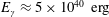 $E_{\unicode[STIX]{x1D6FE}}\approx 5\times 10^{40}~\text{erg}$
radiated during the gamma-ray events for the same period (estimated using (4.13). Thus only a tiny fraction of the magnetic energy dissipated in the polar region results in flares. The kinetic beaming alone cannot explain this disparity as its beaming factor is found to be only approximately
$E_{\unicode[STIX]{x1D6FE}}\approx 5\times 10^{40}~\text{erg}$
radiated during the gamma-ray events for the same period (estimated using (4.13). Thus only a tiny fraction of the magnetic energy dissipated in the polar region results in flares. The kinetic beaming alone cannot explain this disparity as its beaming factor is found to be only approximately
 $f_{b}=0.1$
(see § 4.2). However, there are number of other possible reasons.
$f_{b}=0.1$
(see § 4.2). However, there are number of other possible reasons.
The potential drop across the whole polar zone is only just above that required to explain the peak energy of the flares. If typical current sheets are rather small compared to the size of the polar zone, their potential drops may be significantly lower, resulting in a lower maximum energy of accelerated particles and hence a lower peak energy of the flares. Events with
 ${\mathcal{E}}_{\unicode[STIX]{x1D708}}<100~\text{MeV}$
would be much less prominent due to the much higher mean flux from the nebula at these energies.
${\mathcal{E}}_{\unicode[STIX]{x1D708}}<100~\text{MeV}$
would be much less prominent due to the much higher mean flux from the nebula at these energies.
The typical plasma magnetisation
 $\unicode[STIX]{x1D70E}$
could be too high, leading to very hard spectra. In order to understand why this could be a problem, let us consider a monoenergetic spectrum. In this case, all particles would have the Lorentz factor
$\unicode[STIX]{x1D70E}$
could be too high, leading to very hard spectra. In order to understand why this could be a problem, let us consider a monoenergetic spectrum. In this case, all particles would have the Lorentz factor
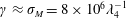 $\unicode[STIX]{x1D6FE}\approx \unicode[STIX]{x1D70E}_{M}=8\times 10^{6}\unicode[STIX]{x1D706}_{4}^{-1}$
, which is well below the
$\unicode[STIX]{x1D6FE}\approx \unicode[STIX]{x1D70E}_{M}=8\times 10^{6}\unicode[STIX]{x1D706}_{4}^{-1}$
, which is well below the
 $\unicode[STIX]{x1D6FE}=\,\text{few}\times 10^{9}$
required for the flare electrons. In order to illustrate this for the case of a power-law spectrum, we can rewrite (4.24) as
$\unicode[STIX]{x1D6FE}=\,\text{few}\times 10^{9}$
required for the flare electrons. In order to illustrate this for the case of a power-law spectrum, we can rewrite (4.24) as
 $$\begin{eqnarray}\unicode[STIX]{x1D6FE}_{\text{max}}^{p}=\unicode[STIX]{x1D70E}_{M}\frac{2-p}{p-1}\unicode[STIX]{x1D6FE}_{\text{min}}^{p-1}\end{eqnarray}$$
and consider
 $p=1.1$
as an example of very hard spectrum corresponding to
$p=1.1$
as an example of very hard spectrum corresponding to
 $\unicode[STIX]{x1D70E}>100$
. Even for
$\unicode[STIX]{x1D70E}>100$
. Even for
 $\unicode[STIX]{x1D706}_{4}=1$
and
$\unicode[STIX]{x1D706}_{4}=1$
and
 $\unicode[STIX]{x1D6FE}_{\text{min}}=10^{5}$
this gives
$\unicode[STIX]{x1D6FE}_{\text{min}}=10^{5}$
this gives
 $\unicode[STIX]{x1D6FE}_{\text{max}}\approx 4\times 10^{7}$
only. In a magnetic field of strength
$\unicode[STIX]{x1D6FE}_{\text{max}}\approx 4\times 10^{7}$
only. In a magnetic field of strength
 $B=1~\text{mG}$
the synchrotron emission of such particles would not extend much above the cutoff energy of
$B=1~\text{mG}$
the synchrotron emission of such particles would not extend much above the cutoff energy of
 ${\mathcal{E}}_{\unicode[STIX]{x1D708}}\approx 30~\text{keV}$
.
${\mathcal{E}}_{\unicode[STIX]{x1D708}}\approx 30~\text{keV}$
.
In the polar zone, the shocked wind plasma flows predominantly along the polar axis, with the initial half-opening angle
 $\unicode[STIX]{x1D703}\approx \unicode[STIX]{x1D703}_{p}$
. The polar axis of the Crab pulsar makes an angle of approximately
$\unicode[STIX]{x1D703}\approx \unicode[STIX]{x1D703}_{p}$
. The polar axis of the Crab pulsar makes an angle of approximately
 $60^{\circ }$
to the line of sight (Ng & Romani Reference Ng and Romani2004). Downstream of the termination shock we expect its speed to be very close to the speed of light, with
$60^{\circ }$
to the line of sight (Ng & Romani Reference Ng and Romani2004). Downstream of the termination shock we expect its speed to be very close to the speed of light, with
 $\unicode[STIX]{x1D6FE}\gg 1$
, and its emission strongly beamed in the direction of motion. As a result, its observed emission is Doppler dimmed. Although, the flow eventually slows down to the characteristic speed
$\unicode[STIX]{x1D6FE}\gg 1$
, and its emission strongly beamed in the direction of motion. As a result, its observed emission is Doppler dimmed. Although, the flow eventually slows down to the characteristic speed
 $v_{j}\approx 0.4c$
of Crab’s polar jet (Hester et al.
Reference Hester, Mori, Burrows, Gallagher, Graham, Halverson, Kader, Michel and Scowen2002), we may still expect that most of the emission associated with magnetic reconnection in the polar zone is beamed away from the Earth.
$v_{j}\approx 0.4c$
of Crab’s polar jet (Hester et al.
Reference Hester, Mori, Burrows, Gallagher, Graham, Halverson, Kader, Michel and Scowen2002), we may still expect that most of the emission associated with magnetic reconnection in the polar zone is beamed away from the Earth.
Thus, the observed gamma-ray flares seem to be associated with rather exceptional circumstances when the reconnection region is rather large in terms of its potential drop, its magnetisation is rather low, presumably due to some previous phases of reconnection, and its velocity is either strongly reduced or directed towards the line of sight, e.g. due to interaction with its highly disturbed low-
 $\unicode[STIX]{x1D70E}$
surrounding. High-resolution RMHD or PIC simulations of the polar region are required to clarify this issue.
$\unicode[STIX]{x1D70E}$
surrounding. High-resolution RMHD or PIC simulations of the polar region are required to clarify this issue.
While the shock model of Kennel & Coroniti (Reference Kennel and Coroniti1984b
) allows a simple prescription for the emission of the Crab Nebula, the magnetic reconnection does not. It remains to be seen what kind of integral particle spectra can be produced in this model. The model will have to incorporate two-component (the polar zone plus the equatorial zone) structure of pulsar winds as they inject plasmas with very different physical parameters. Moreover, due to the anisotropy of the wind power the striped component is expected to carry most energy of the energy and the magnetisation of plasma it injects into the nebula is quite low
 $\unicode[STIX]{x1D70E}<1$
. For such a magnetisation the spectrum of non-thermal electrons accelerated via magnetic reconnection is expected to be very soft
$\unicode[STIX]{x1D70E}<1$
. For such a magnetisation the spectrum of non-thermal electrons accelerated via magnetic reconnection is expected to be very soft
 $p>4$
, in fact too soft to agree with the observations. This suggests that another acceleration mechanism is at work there, presumably the second-order Fermi mechanism involving plasma turbulence.
$p>4$
, in fact too soft to agree with the observations. This suggests that another acceleration mechanism is at work there, presumably the second-order Fermi mechanism involving plasma turbulence.
Based on the results of PIC simulations of shocks in a relativistic magnetised plasma the termination shock of pulsar winds only thermalises the plasma (except the very narrow section near the equator where the first-order Fermi mechanism may operate). This conclusion makes observational identification of the termination shock and studying of its broadband spectrum particularly important. So far we have two candidates: the X-ray ring of the Crab Nebula and its inner knot. In both cases the broadband spectrum is not known. The inner ring may correspond to the narrow equatorial section of the termination shock where the emitting particles are accelerated via the Fermi mechanism, whereas the inner knot corresponds to the high latitude part of the termination shock, terminating the striped section of the pulsar wind, where the theory predicts a relativistic Maxwellian spectrum of the emitting particles.
6.3 Implications for other high-energy sources: acceleration by shocks and/or magnetic reconnection
The Crab Nebula is the paragon of the high-energy astrophysical source. Both the observational and theoretical studies of the Crab Nebula have made a very strong impact on the development of high-energy astrophysics in general. Given the proximity of this object and the unprecedented level of detail it offers, one would expect that it will retain its special place. Many other astrophysical phenomena involve flows of highly magnetised relativistic plasma. Most of all, these are active galactic nuclei and presumably gamma-ray bursts as well (e.g., Blandford & Znajek Reference Blandford and Znajek1977; Usov Reference Usov1992; Thompson, Chang & Quataert Reference Thompson, Chang and Quataert2004; Lyutikov Reference Lyutikov2006b ; Komissarov & Barkov Reference Komissarov and Barkov2007), which involve production of relativistic jets from compact magnetised rotators, black holes and neutron stars.
Most of the emission coming from AGN jets is non-thermal, which makes the issue of non-thermal particle acceleration central to these studies. For a long time it was believed that such particles are accelerated at shocks, which naturally emerge in supersonic flows. However, the recent PIC simulations of a relativistic plasma place severe constrains on the shock acceleration mechanism in a magnetised relativistic plasma – acceleration operates only in the case of weak magnetisation,
 $\unicode[STIX]{x1D70E}<10^{-2}$
. Although these results are often ignored and the shock model is still in use, the high-energy astrophysics is in a mini-crisis. Relativistic magnetic reconnection may be offering a way out this crisis both in the case of AGN (e.g. Blandford Reference Blandford, Gilfanov, Sunyeav and Churazov2002; Lyutikov Reference Lyutikov2003; Uzdensky Reference Uzdensky2011; Sironi, Petropoulou & Giannios Reference Sironi, Petropoulou and Giannios2015) and GRBs (e.g. Lyutikov, Pariev & Blandford Reference Lyutikov, Pariev and Blandford2003; Lyutikov Reference Lyutikov2006b
). It is quite possible that the high-energy flares of AGNs as well as the spikes in the light curves of GRBs are similar in nature to the flares of Crab Nebula (Lyutikov Reference Lyutikov2006a
; Giannios, Uzdensky & Begelman Reference Giannios, Uzdensky and Begelman2010; Clausen-Brown & Lyutikov Reference Clausen-Brown and Lyutikov2012) and hence exploring the magnetic reconnection model for the emission of the Crab Nebula will have important implications in the astrophysics of AGNs and GRBs once again.
$\unicode[STIX]{x1D70E}<10^{-2}$
. Although these results are often ignored and the shock model is still in use, the high-energy astrophysics is in a mini-crisis. Relativistic magnetic reconnection may be offering a way out this crisis both in the case of AGN (e.g. Blandford Reference Blandford, Gilfanov, Sunyeav and Churazov2002; Lyutikov Reference Lyutikov2003; Uzdensky Reference Uzdensky2011; Sironi, Petropoulou & Giannios Reference Sironi, Petropoulou and Giannios2015) and GRBs (e.g. Lyutikov, Pariev & Blandford Reference Lyutikov, Pariev and Blandford2003; Lyutikov Reference Lyutikov2006b
). It is quite possible that the high-energy flares of AGNs as well as the spikes in the light curves of GRBs are similar in nature to the flares of Crab Nebula (Lyutikov Reference Lyutikov2006a
; Giannios, Uzdensky & Begelman Reference Giannios, Uzdensky and Begelman2010; Clausen-Brown & Lyutikov Reference Clausen-Brown and Lyutikov2012) and hence exploring the magnetic reconnection model for the emission of the Crab Nebula will have important implications in the astrophysics of AGNs and GRBs once again.
Acknowledgements
We would like to thank R. Blandford, K. Nalewajko, D. Uzdensky and J. Zrake for stimulating discussions. This research was supported via NASA grant NNX12AF92G, NSF grant AST-1306672 and DoE grant 108483. O.P. is supported by the ERC Synergy Grant ‘BlackHoleCam – Imaging the Event Horizon of Black Holes’ (grant 610058). S.S.K. is supported by the STFC grant ST/N000676/1. The simulations were performed on XSEDE resources under contract no. TG-AST120010, and on NASA High-End Computing (HEC) resources through the NASA Advanced Supercomputing (NAS) Division at Ames Research Center. M.L. would like to thank for hospitality Osservatorio Astrofisico di Arcetri and Institut de Ciencies de l’Espai, where large parts of this work were conducted. S.S.K. thanks Purdue University for hospitality during sabbatical in 2014 when a significant part of this work was carried out.


