


1 Introduction
1.1 Background
Sometimes constraints are maintained effortlessly, an example being the constraint on the magnetic field,  $\unicode[STIX]{x1D735}\boldsymbol{\cdot }\boldsymbol{B}=0$, in electrodynamics which if initially true remains true, while alternatively in most cases dynamical equations must be modified to maintain constraints, an example being $\unicode[STIX]{x1D735}\boldsymbol{\cdot }\boldsymbol{v}=0$ in fluid mechanics. The need to apply constraints arises in a variety of contexts, ranging from gauge field theories (e.g. Sundermeyer Reference Sundermeyer1982) to optimization and control (e.g. Bloch Reference Bloch2002). A very common approach is to use the method of Lagrange multipliers, which is taught in standard physics curricula for imposing holonomic constraints in mechanical systems. Alternatively, Dirac (Reference Dirac1950), in pursuit of his goal of quantizing gauge field theories, introduced a method that uses the Poisson bracket.
The purpose of the present article is to explore different methods for imposing the compressibility constraint in ideal (dissipation-free) fluid mechanics and its extension to magnetohydrodynamics (MHD), classical field theories intended for classical purposes. This endeavour is richer than might be expected because the different methods of constraint can be applied to the fluid in either the Lagrangian (material) description or the Eulerian (spatial) description, and the constraint methods have different manifestations in the Lagrangian (action principle) and Hamiltonian formulations. Although Lagrange’s multiplier is widely appreciated, it is not so well known that he used it long ago for imposing the incompressibility constraint for a fluid in the Lagrangian variable description (Lagrange Reference Lagrange1788). More recently, Dirac’s method was applied for imposing incompressibility within the Eulerian variable description, first in Nguyen & Turski (Reference Nguyen and Turski1999, Reference Nguyen and Turski2001) and followed up in several works (Morrison, Lebovitz & Biello Reference Morrison, Lebovitz and Biello2009; Tassi, Chandre & Morrison Reference Tassi, Chandre and Morrison2009; Chandre, Morrison & Tassi Reference Chandre, Morrison and Tassi2012, Reference Chandre, Morrison and Tassi2014; Chandre et al. Reference Chandre, de Guillebon, Back, Tassi and Morrison2013). Given that a Lagrangian conservation law is not equivalent to an Eulerian conservation law, it remains to elucidate the interplay between the methods of constraint and the variables used for the description of the fluid. Thus we have three dichotomies: the Lagrangian versus Eulerian fluid descriptions, Lagrange multiplier versus Dirac constraint methods and Lagrangian versus Hamiltonian formalisms. It is the elucidation of the interplay between these, along with generalizing previous results, that is the present goal.
It is well known that a free particle with holonomic constraints, imposed by the method of Lagrange multipliers, is a geodesic flow. Indeed, Lagrange essentially observed this in Lagrange (Reference Lagrange1788) for the ideal fluid when he imposed the incompressibility constraint by his method. Lagrange did this in the Lagrangian description by imposing the constraint that the map from the initial positions of fluid elements to their positions at time  $t$ preserves volume, and he did this by the method of Lagrange multipliers. It is worth noting that Lagrange knew the Lagrange multiplier turns out to be the pressure, but he had trouble solving for it. Lagrange’s calculation was placed in a geometrical setting by Arnold (Reference Arnold1966) (see also appendix 2 of Arnold (Reference Arnold1978)), where the constrained maps from the initial conditions were first referred to as volume preserving diffeomorphisms in this context. Given this background, in our investigation of the three dichotomies described above we emphasize geodesic flow.
For later use we record here the incompressible Euler equations for the case with constant density and the case where density is advected. The equations of motion, allowing for density advection, are given by
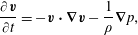 $$\begin{eqnarray}\displaystyle & \displaystyle \frac{\unicode[STIX]{x2202}\boldsymbol{v}}{\unicode[STIX]{x2202}t}=-\boldsymbol{v}\boldsymbol{\cdot }\unicode[STIX]{x1D735}\boldsymbol{v}-\frac{1}{\unicode[STIX]{x1D70C}}\unicode[STIX]{x1D735}p, & \displaystyle\end{eqnarray}$$
 $$\begin{eqnarray}\displaystyle & \displaystyle \unicode[STIX]{x1D735}\boldsymbol{\cdot }\boldsymbol{v}=0, & \displaystyle\end{eqnarray}$$
 $$\begin{eqnarray}\displaystyle & \displaystyle \frac{\unicode[STIX]{x2202}\unicode[STIX]{x1D70C}}{\unicode[STIX]{x2202}t}=-\boldsymbol{v}\boldsymbol{\cdot }\unicode[STIX]{x1D735}\unicode[STIX]{x1D70C}, & \displaystyle\end{eqnarray}$$
 where  $\boldsymbol{v}(\boldsymbol{x},t)$ is the velocity field, $\unicode[STIX]{x1D70C}(\boldsymbol{x},t)$ is the mass density, $p(\boldsymbol{x},t)$ is the pressure and $\boldsymbol{x}\in D$, the region occupied by the fluid. These equations are generally subject to the free-slip boundary condition $\boldsymbol{n}\boldsymbol{\cdot }\boldsymbol{v}|_{\unicode[STIX]{x2202}D}=0$, where $\boldsymbol{n}$ is normal to the boundary of $D$. The pressure field that enforces the constraint (1.2) is obtained by setting $\unicode[STIX]{x2202}(\unicode[STIX]{x1D735}\boldsymbol{\cdot }\boldsymbol{v})\unicode[STIX]{x2202}t=0$, which implies
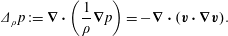 $$\begin{eqnarray}\unicode[STIX]{x1D6E5}_{\unicode[STIX]{x1D70C}}p:=\unicode[STIX]{x1D735}\boldsymbol{\cdot }\left(\frac{1}{\unicode[STIX]{x1D70C}}\unicode[STIX]{x1D735}p\right)=-\unicode[STIX]{x1D735}\boldsymbol{\cdot }(\boldsymbol{v}\boldsymbol{\cdot }\unicode[STIX]{x1D735}\boldsymbol{v}).\end{eqnarray}$$
 For reasonable assumptions on  $\unicode[STIX]{x1D70C}$ and boundary conditions, equation (1.4) is a well-posed elliptic equation (see e.g. Evans (Reference Evans2010)), so we can write
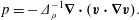 $$\begin{eqnarray}p=-\unicode[STIX]{x1D6E5}_{\unicode[STIX]{x1D70C}}^{-1}\unicode[STIX]{x1D735}\boldsymbol{\cdot }(\boldsymbol{v}\boldsymbol{\cdot }\unicode[STIX]{x1D735}\boldsymbol{v}).\end{eqnarray}$$
 For the case where  $\unicode[STIX]{x1D70C}$ is constant we have the usual Green’s function expression
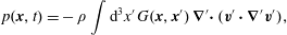 $$\begin{eqnarray}p(\boldsymbol{x},t)=-\,\unicode[STIX]{x1D70C}\int \text{d}^{3}x^{\prime }\,G(\boldsymbol{x},\boldsymbol{x}^{\prime })\,\unicode[STIX]{x1D735}^{\prime }\!\boldsymbol{\cdot }(\boldsymbol{v}^{\prime }\boldsymbol{\cdot }\unicode[STIX]{x1D735}^{\prime }\boldsymbol{v}^{\prime }),\end{eqnarray}$$
 where  $G$ is consistent with Neumann boundary conditions (Orszag, Israeli & Deville Reference Orszag, Israeli and Deville1986) and $\boldsymbol{v}^{\prime }=\boldsymbol{v}(\boldsymbol{x}^{\prime },t)$. Insertion of (1.6) into (1.1) gives
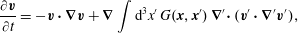 $$\begin{eqnarray}\frac{\unicode[STIX]{x2202}\boldsymbol{v}}{\unicode[STIX]{x2202}t}=-\boldsymbol{v}\boldsymbol{\cdot }\unicode[STIX]{x1D735}\boldsymbol{v}+\unicode[STIX]{x1D735}\int \text{d}^{3}x^{\prime }\,G(\boldsymbol{x},\boldsymbol{x}^{\prime })\,\unicode[STIX]{x1D735}^{\prime }\!\boldsymbol{\cdot }(\boldsymbol{v}^{\prime }\boldsymbol{\cdot }\unicode[STIX]{x1D735}^{\prime }\boldsymbol{v}^{\prime }),\end{eqnarray}$$
 which is a closed system for  $\boldsymbol{v}(\boldsymbol{x},t)$.
For MHD, equation (1.1) has the additional term  $(\unicode[STIX]{x1D735}\times \boldsymbol{B})\times \boldsymbol{B}/\unicode[STIX]{x1D70C}$ added to the right-hand side. Consequently for this model, the source of (1.5) is modified by the addition of this term to $-\boldsymbol{v}\boldsymbol{\cdot }\unicode[STIX]{x1D735}\boldsymbol{v}$.
1.2 Overview
Section 2 contains material that serves as a guide for navigating the more complicated calculations to follow. We first consider the various approaches to constraints in the finite-dimensional context in §§ 2.1 and 2.3. Section 2.1 briefly covers conventional material about holonomic constraints by Lagrange multipliers – here the reader is reminded how the free particle with holonomic constraints amounts to geodesic flow. Section 2.2 begins with the phase space action principle, whence the Dirac bracket for constraints is obtained by Lagrange’s multiplier method, but with phase space constraints as opposed to the usual holonomic configuration space constraints used in conjunction with Hamilton’s principle of mechanics, as described in § 2.1. Next, in § 2.3, we compare the results of §§ 2.1 and 2.3 and show how conventional holonomic constraints can be enforced by Dirac’s method. Contrary to Lagrange’s method, here we obtain explicit expressions, ones that do not appear in conventional treatments, for the Christoffel symbol and the normal force entirely in terms of the original Euclidean coordinates and constraints. Section 2 is completed with § 2.4, where the previous ideas are revisited in the  $d+1$ field theory context in preparation for the fluid and MHD calculations. Holonomic constraints, Dirac brackets, with local or non-local constraints, and geodesic flow are treated.
In § 3 we first consider the compressible (unconstrained) fluid and MHD versions of Hamilton’s variational principle, the principle of least action, with Lagrange’s Lagrangian in the Lagrangian description. From this we obtain in § 3.2 the canonical Hamiltonian field theoretic form in the Lagrangian variable description, which is transformed in § 3.3, via the mapping from Lagrangian to Eulerian variables, to the noncanonical Eulerian form. Section 3 is completed by an in depth comparison of constants of motion in the Eulerian and Lagrangian descriptions, which surprisingly does not seem to appear in fluid mechanics or plasma physics textbooks. The material of this section is necessary for understanding the different manifestations of constraints in our dichotomies.
Section 4 begins with § 4.1 that reviews Lagrange’s original calculations. Because the incompressibility constraint he imposes is holonomic and there are no additional forces, his equations describe infinite-dimensional geodesics flow on volume preserving maps. The remaining portion of this section contains the most substantial calculations of the paper. In § 4.2 for the first time Dirac’s theory is applied to enforce incompressibility in the Lagrangian variable description. This results in a new Dirac bracket that generates volume preserving flows. As in § 2.3.1, which serves as a guide, the equations of motion generated by the bracket are explicit and contain only the constraints and original variables. Next, in § 4.3, a reduction from Lagrangian to Eulerian variables is made, resulting in a new Eulerian variable Poisson bracket that allows for density advection while preserving incompressibility. This was an heretofore unsolved problem. Section 4.4 ties together the results of §§ 4.2, 4.3 and 3.4. Here both the Eulerian and Lagrangian Dirac constraint theories are compared after they are evaluated on their respective constraints, simplifying their equations of motion. Because Lagrangian and Eulerian conservation laws are not identical, we see that there are differences. Section 4 concludes in § 4.5 with a discussion of the full algebra of invariants, that of the ten parameter Galilean group, for both the Lagrangian and Eulerian descriptions. In addition the Casimir invariants of the theories are discussed.
The paper concludes with § 5, where we briefly summarize our results and speculate about future possibilities.
2 Constraint methods
2.1 Holonomic constraints by Lagrange’s multiplier method
Of interest are systems with Lagrangians of the form  $L(\dot{q},q)$ where the overdot denotes time differentiation and $q=(q^{1},q^{2},\ldots ,q^{N})$. Because non-autonomous systems could be included by appending an additional degree of freedom, explicit time dependence is not included in $L$.
$L$.
Given the Lagrangian, the equations of motion are obtained according to Hamilton’s principle by variation of the action
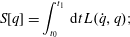 $$\begin{eqnarray}S[q]=\int _{t_{0}}^{t_{1}}\,\text{d}t\,L(\dot{q},q);\end{eqnarray}$$
i.e.
 $$\begin{eqnarray}\unicode[STIX]{x1D6FF}S[q;\unicode[STIX]{x1D6FF}q]:=\frac{\text{d}}{\text{d}\unicode[STIX]{x1D716}}S[q+\unicode[STIX]{x1D716}\unicode[STIX]{x1D6FF}q]\Big|_{\unicode[STIX]{x1D716}=0}=\int _{t_{0}}^{t_{1}}\,\text{d}t\left(\frac{\text{d}}{\,\text{d}t}\frac{\unicode[STIX]{x2202}L}{\unicode[STIX]{x2202}\dot{q}^{i}}-\frac{\unicode[STIX]{x2202}L}{\unicode[STIX]{x2202}q^{i}}\right)\unicode[STIX]{x1D6FF}q^{i}=\int _{t_{0}}^{t_{1}}\,\text{d}t\frac{\unicode[STIX]{x1D6FF}S[q]}{\unicode[STIX]{x1D6FF}q^{i}(t)}\,\unicode[STIX]{x1D6FF}q^{i}=0,\end{eqnarray}$$
 for all variations  $\unicode[STIX]{x1D6FF}q(t)$ satisfying $\unicode[STIX]{x1D6FF}q(t_{0})=\unicode[STIX]{x1D6FF}q(t_{1})=0$, implies Lagrange’s equations of motion, i.e.
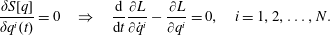 $$\begin{eqnarray}\frac{\unicode[STIX]{x1D6FF}S[q]}{\unicode[STIX]{x1D6FF}q^{i}(t)}=0\quad \Rightarrow \quad \frac{\text{d}}{\text{d}t}\frac{\unicode[STIX]{x2202}L}{\unicode[STIX]{x2202}\dot{q}^{i}}-\frac{\unicode[STIX]{x2202}L}{\unicode[STIX]{x2202}q^{i}}=0,\quad i=1,2,\ldots ,N.\end{eqnarray}$$
 Holonomic constraints are real-valued functions of the form  $C^{A}(q)$, $A=1,2,\ldots ,M$, which are desired to be constant on trajectories. Lagrange’s method for implementing such constraints is to add them to the action and vary as follows:
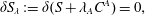 $$\begin{eqnarray}\unicode[STIX]{x1D6FF}S_{\unicode[STIX]{x1D706}}:=\unicode[STIX]{x1D6FF}(S+\unicode[STIX]{x1D706}_{A}C^{A})=0,\end{eqnarray}$$
yielding the equations of motion
 $$\begin{eqnarray}\frac{\unicode[STIX]{x1D6FF}S_{\unicode[STIX]{x1D706}}[q]}{\unicode[STIX]{x1D6FF}q^{i}(t)}=0\quad \Rightarrow \quad \frac{\text{d}}{\,\text{d}t}\frac{\unicode[STIX]{x2202}L}{\unicode[STIX]{x2202}\dot{q}^{i}}-\frac{\unicode[STIX]{x2202}L}{\unicode[STIX]{x2202}q^{i}}=\unicode[STIX]{x1D706}_{A}\frac{\unicode[STIX]{x2202}C^{A}}{\unicode[STIX]{x2202}q^{i}},\quad i=1,2,\ldots ,N,\end{eqnarray}$$
 with the forces of constraint residing on the right-hand side of (2.5). Observe in (2.4) and (2.5) repeated sum notation is implied for the index  $A$. The $N$ equations of (2.5) with the $M$ numerical values of the constraints $C^{A}(q)=C_{0}^{A}$, determine the $N+M$ unknowns $\{q^{i}\}$ and $\{\unicode[STIX]{x1D706}_{A}\}$. In practice, because solving for the Lagrange multipliers can be difficult an alternative procedure, an example of which we describe in § 2.1.1, is used.
We will see in § 4.1 that the field theoretic version of this method is how Lagrange implemented the incompressibility constraint for fluid flow. For the purpose of illustration and in preparation for later development, we consider a finite-dimensional analogue of Lagrange’s treatment.
2.1.1 Holonomic constraints and geodesic flow via Lagrange
Consider  $N$ non-interacting bodies each of mass $m_{i}$ in the Euclidian configuration space $\mathbb{E}^{3N}$ with Cartesian coordinates $\boldsymbol{q}_{i}=(q_{xi},q_{yi},q_{zi})$, where as in § 2.1 $i=1,2,\ldots ,N$, but our configuration space has dimension $3N$. The Lagrangian for this system is given by the usual kinetic energy,
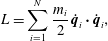 $$\begin{eqnarray}L=\mathop{\sum }_{i=1}^{N}\frac{m_{i}}{2}\,\dot{\boldsymbol{q}}_{i}\boldsymbol{\cdot }\dot{\boldsymbol{q}}_{i},\end{eqnarray}$$
 with the usual ‘dot’ product. The Euler–Lagrange equations for this system, equation (2.3), are the uninteresting system of  $N$ free particles. As in § 2.1 we constrain this system by adding constraints $C^{A}(\boldsymbol{q}_{1},\boldsymbol{q}_{2},\ldots ,\boldsymbol{q}_{N})$, where again $A=1,2,\ldots ,M$, leading to the equations
 $$\begin{eqnarray}m_{i}\ddot{\boldsymbol{q}}_{i}=\unicode[STIX]{x1D706}_{A}\frac{\unicode[STIX]{x2202}C^{A}}{\unicode[STIX]{x2202}\boldsymbol{q}_{i}}.\end{eqnarray}$$
 Instead of solving the  $3N$ equations of (2.7) together with the $M$ numerical values of the constraints, in order to determine the unknowns $\boldsymbol{q}_{i}$ and $\unicode[STIX]{x1D706}_{A}$, we recall the alternative procedure, which dates back to Lagrange (see e.g. § IV of Lagrange (Reference Lagrange1788)) and has been taught to physics students for generations (see e.g. Whittaker (Reference Whittaker1917), Corben & Stehle (Reference Corben and Stehle1960)). With the alternative procedure one introduces generalized coordinates that account for the constraints, yielding a smaller system on the constraint manifold, one with the Lagrangian
 $$\begin{eqnarray}L={\textstyle \frac{1}{2}}g_{\unicode[STIX]{x1D707}\unicode[STIX]{x1D708}}(q)\,\dot{q}^{\unicode[STIX]{x1D707}}\dot{q}^{\unicode[STIX]{x1D708}},\quad \unicode[STIX]{x1D707},\unicode[STIX]{x1D708}=1,2\ldots ,3N-M,\end{eqnarray}$$
where
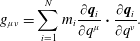 $$\begin{eqnarray}g_{\unicode[STIX]{x1D707}\unicode[STIX]{x1D708}}=\mathop{\sum }_{i=1}^{N}m_{i}\frac{\unicode[STIX]{x2202}\boldsymbol{q}_{i}}{\unicode[STIX]{x2202}q^{\unicode[STIX]{x1D707}}}\boldsymbol{\cdot }\frac{\unicode[STIX]{x2202}\boldsymbol{q}_{i}}{\unicode[STIX]{x2202}q^{\unicode[STIX]{x1D708}}}.\end{eqnarray}$$
Then Lagrange’s equations (2.3) for the Lagrangian (2.13) are the usual equations for geodesic flow
 $$\begin{eqnarray}\ddot{q}^{\unicode[STIX]{x1D707}}+\unicode[STIX]{x1D6E4}_{\unicode[STIX]{x1D6FC}\unicode[STIX]{x1D6FD}}^{\unicode[STIX]{x1D707}}\,\dot{q}^{\unicode[STIX]{x1D6FC}}\dot{q}^{\unicode[STIX]{x1D6FD}}=0,\end{eqnarray}$$
where the Christoffel symbol is as usual
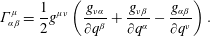 $$\begin{eqnarray}\unicode[STIX]{x1D6E4}_{\unicode[STIX]{x1D6FC}\unicode[STIX]{x1D6FD}}^{\unicode[STIX]{x1D707}}=\frac{1}{2}g^{\unicode[STIX]{x1D707}\unicode[STIX]{x1D708}}\left(\frac{g_{\unicode[STIX]{x1D708}\unicode[STIX]{x1D6FC}}}{\unicode[STIX]{x2202}q^{\unicode[STIX]{x1D6FD}}}+\frac{g_{\unicode[STIX]{x1D708}\unicode[STIX]{x1D6FD}}}{\unicode[STIX]{x2202}q^{\unicode[STIX]{x1D6FC}}}-\frac{g_{\unicode[STIX]{x1D6FC}\unicode[STIX]{x1D6FD}}}{\unicode[STIX]{x2202}q^{\unicode[STIX]{x1D708}}}\right).\end{eqnarray}$$
If the constraints had time dependence, then the procedure would have produced the Coriolis and centripetal forces, as is usually done in textbooks.
Thus, we arrive at the conclusion that free particle dynamics with time-independent holonomic constraints is geodesic flow.
2.2 Dirac’s bracket method
So, a natural question to ask is ‘How does one implement constraints in the Hamiltonian setting, where phase space constraints depend on both the configuration space coordinate  $q$ and the canonical momentum $p$’? (see e.g. Sundermeyer (Reference Sundermeyer1982), Arnold, Kozlov & Neishtadt (Reference Arnold, Kozlov and Neishtadt1980) for a general treatment and Dermaret & Moncrief (Reference Dermaret and Moncrief1980) for a treatment in the context of the ideal fluid and relativity and a selection of earlier references.) To this end we begin with the phase space action principle
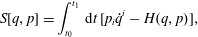 $$\begin{eqnarray}S[q,p]=\int _{t_{0}}^{t_{1}}\,\text{d}t\,[p_{i}\dot{q}^{i}-H(q,p)],\end{eqnarray}$$
 where again repeated sum notation is used for  $i=1,2,\ldots ,N$. Independent variation of $S[q,p]$ with respect to $q$ and $p$, with $\unicode[STIX]{x1D6FF}q(t_{0})=\unicode[STIX]{x1D6FF}q(t_{1})=0$ and no conditions on $\unicode[STIX]{x1D6FF}p$, yields Hamilton’s equations,
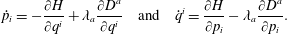
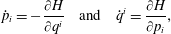 $$\begin{eqnarray}{\dot{p}}_{i}=-\frac{\unicode[STIX]{x2202}H}{\unicode[STIX]{x2202}q^{i}}\quad \text{and}\quad \dot{q}^{i}=\frac{\unicode[STIX]{x2202}H}{\unicode[STIX]{x2202}p_{i}},\end{eqnarray}$$
or equivalently
 $$\begin{eqnarray}{\dot{z}}^{\unicode[STIX]{x1D6FC}}=\{z^{\unicode[STIX]{x1D6FC}},H\},\end{eqnarray}$$
 which is a rewrite of (2.13) in terms of the Poisson bracket on phase space functions  $f$ and $g$,
$g$,
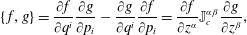 $$\begin{eqnarray}\{\,f,g\}=\frac{\unicode[STIX]{x2202}f}{\unicode[STIX]{x2202}q^{i}}\frac{\unicode[STIX]{x2202}g}{\unicode[STIX]{x2202}p_{i}}-\frac{\unicode[STIX]{x2202}g}{\unicode[STIX]{x2202}q^{i}}\frac{\unicode[STIX]{x2202}f}{\unicode[STIX]{x2202}p_{i}}=\frac{\unicode[STIX]{x2202}f}{\unicode[STIX]{x2202}z^{\unicode[STIX]{x1D6FC}}}\mathbb{J}_{c}^{\unicode[STIX]{x1D6FC}\unicode[STIX]{x1D6FD}}\frac{\unicode[STIX]{x2202}g}{\unicode[STIX]{x2202}z^{\unicode[STIX]{x1D6FD}}},\end{eqnarray}$$
 where in the second equality we have used  $z=(q,p)$, so $\unicode[STIX]{x1D6FC},\unicode[STIX]{x1D6FD}=1,2,\ldots ,2N$ and the cosymplectic form (Poisson matrix) is
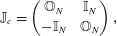 $$\begin{eqnarray}\mathbb{J}_{c}=\left(\begin{array}{@{}cc@{}}\mathbb{O}_{N} & \mathbb{I}_{N}\\ -\mathbb{I}_{N} & \mathbb{O}_{N}\end{array}\right),\end{eqnarray}$$
 with  $\mathbb{O}_{N}$ being an $N\times N$ block of zeros and $\mathbb{I}_{N}$ being the $N\times N$ identity.
Proceeding as in § 2.1, albeit with phase space constraints  $D^{a}(q,p)$, $a=1,2,\ldots ,2M<2N$, we vary
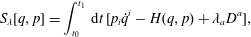 $$\begin{eqnarray}S_{\unicode[STIX]{x1D706}}[q,p]=\int _{t_{0}}^{t_{1}}\,\text{d}t\,[p_{i}\dot{q}^{i}-H(q,p)+\unicode[STIX]{x1D706}_{a}D^{a}],\end{eqnarray}$$
and obtain
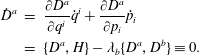
 $$\begin{eqnarray}{\dot{p}}_{i}=-\frac{\unicode[STIX]{x2202}H}{\unicode[STIX]{x2202}q^{i}}+\unicode[STIX]{x1D706}_{a}\frac{\unicode[STIX]{x2202}D^{a}}{\unicode[STIX]{x2202}q^{i}}\quad \text{and}\quad \dot{q}^{i}=\frac{\unicode[STIX]{x2202}H}{\unicode[STIX]{x2202}p_{i}}-\unicode[STIX]{x1D706}_{a}\frac{\unicode[STIX]{x2202}D^{a}}{\unicode[STIX]{x2202}p_{i}}.\end{eqnarray}$$
 Next, enforcing  ${\dot{D}}^{a}=0$ for all $a$, will ensure that the constraints stay put. Whence, differentiating the $D^{a}$ and using (2.18) yields
 $$\begin{eqnarray}\displaystyle {\dot{D}}^{a} & = & \displaystyle \frac{\unicode[STIX]{x2202}D^{a}}{\unicode[STIX]{x2202}q^{i}}\dot{q}^{i}+\frac{\unicode[STIX]{x2202}D^{a}}{\unicode[STIX]{x2202}p_{i}}{\dot{p}}_{i}\nonumber\\ \displaystyle & = & \displaystyle \{D^{a},H\}-\unicode[STIX]{x1D706}_{b}\{D^{a},D^{b}\}\equiv 0.\end{eqnarray}$$
 We assume  $\mathbb{D}^{ab}:=\{D^{a},D^{b}\}$ has an inverse, $\mathbb{D}_{ab}^{-1}$, which requires there be an even number of constraints, $a,b=1,2,\ldots ,2M$, because odd antisymmetric matrices have zero determinant. Then upon solving (2.19) for $\unicode[STIX]{x1D706}_{b}$ and inserting the result into (2.18) gives
 $$\begin{eqnarray}{\dot{z}}^{\unicode[STIX]{x1D6FC}}=\{z^{\unicode[STIX]{x1D6FC}},H\}-\mathbb{D}_{ab}^{-1}\{z^{\unicode[STIX]{x1D6FC}},D^{a}\}\{D^{b},H\}.\end{eqnarray}$$
From (2.20), we obtain a generalization of the Poisson bracket, the Dirac bracket,
 $$\begin{eqnarray}\{\,f,g\}_{\ast }=\{\,f,g\}-\mathbb{D}_{ab}^{-1}\{\,f,D^{a}\}\{D^{b},g\}.\end{eqnarray}$$
which has the degeneracy property
 $$\begin{eqnarray}\{\,f,D^{a}\}_{\ast }\equiv 0.\end{eqnarray}$$
 for all functions  $f$ and indices $a=1,2,\ldots ,2M$.
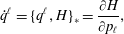
The generation of the equations of motion via a Dirac bracket, i.e.
 $$\begin{eqnarray}{\dot{z}}^{\unicode[STIX]{x1D6FC}}=\{z^{\unicode[STIX]{x1D6FC}},H\}_{\ast },\end{eqnarray}$$
 which is equivalent to (2.20), has the advantage that the Lagrange multipliers  $\unicode[STIX]{x1D706}_{A}$ have been eliminated from the theory.
Note, although the above construction of the Dirac bracket is based on the canonical bracket of (2.15), his construction results in a valid Poisson bracket if one starts from any valid Poisson bracket (cf. (2.76) of §§ 2.4 and 3.3), which need not have a Poisson matrix of the form of (2.16) (see e.g. Morrison et al. (Reference Morrison, Lebovitz and Biello2009)). We will use such a bracket in § 4.3 when we apply constraints by Dirac’s method in the Eulerian variable picture. Also note, for our purposes it is not necessary to describe primary versus secondary constraints (although we use the latter), and the notions of weak versus strong equality. We refer the reader to Dirac (Reference Dirac1950), Sudarshan & Makunda (Reference Sudarshan and Makunda1974), Hanson, Regge & Teitleboim (Reference Hanson, Regge and Teitleboim1976) and Sundermeyer (Reference Sundermeyer1982) for treatment of these concepts.
2.3 Holonomic constraints by Dirac’s bracket method
A connection between the approaches of Lagrange and Dirac can be made. From a set of Lagrangian constraints  $C^{A}(q)$, where $A=1,2,\ldots ,M$, one can construct an additional $M$ constraints by differentiation,
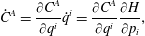 $$\begin{eqnarray}{\dot{C}}^{A}=\frac{\unicode[STIX]{x2202}C^{A}}{\unicode[STIX]{x2202}q^{i}}\dot{q}^{i}=\frac{\unicode[STIX]{x2202}C^{A}}{\unicode[STIX]{x2202}q^{i}}\frac{\unicode[STIX]{x2202}H}{\unicode[STIX]{x2202}p_{i}},\end{eqnarray}$$
where the second equality is possible if (2.3) possesses the Legendre transformation to the Hamiltonian form. In this way we obtain an even number of constraints
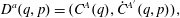 $$\begin{eqnarray}D^{a}(q,p)=(C^{A}(q),{\dot{C}}^{A^{\prime }}(q,p)),\end{eqnarray}$$
 where  $A=1,2,\ldots ,M$, $A^{\prime }=M+1,M+2,\ldots ,2M$ and $a=1,2,\ldots ,2M$.
With the constraints of (2.25) the bracket  $\mathbb{D}^{ab}=\{D^{a},D^{b}\}$ needed to construct (2.21) is easily obtained,
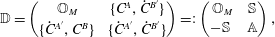 $$\begin{eqnarray}\mathbb{D}=\left(\begin{array}{@{}cc@{}}\mathbb{ O}_{M} & \{C^{A},{\dot{C}}^{B^{\prime }}\}\\ \{{\dot{C}}^{A^{\prime }},C^{B}\} & \{{\dot{C}}^{A^{\prime }},{\dot{C}}^{B^{\prime }}\}\end{array}\right)=:\left(\begin{array}{@{}cc@{}}\,\mathbb{O}_{M} & \mathbb{S}\\ \!-\mathbb{S} & \mathbb{A}\end{array}\right),\end{eqnarray}$$
 where  $\mathbb{O}_{M}$ is an $M\times M$ block of zeros and $\mathbb{S}$ is the following $M\times M$ symmetric matrix with elements
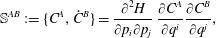 $$\begin{eqnarray}\mathbb{S}^{AB}:=\{C^{A},{\dot{C}}^{B}\}=\frac{\unicode[STIX]{x2202}^{2}H}{\unicode[STIX]{x2202}p_{i}\unicode[STIX]{x2202}p_{j}}\,\frac{\unicode[STIX]{x2202}C^{A}}{\unicode[STIX]{x2202}q^{i}}\frac{\unicode[STIX]{x2202}C^{B}}{\unicode[STIX]{x2202}q^{j}},\end{eqnarray}$$
 and  $\mathbb{A}$ is the following $M\times M$ antisymmetric matrix with elements
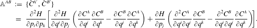 $$\begin{eqnarray}\displaystyle \mathbb{A}^{AB} & := & \displaystyle \{{\dot{C}}^{A^{\prime }},{\dot{C}}^{B^{\prime }}\}\nonumber\\ \displaystyle & = & \displaystyle \frac{\unicode[STIX]{x2202}^{2}H}{\unicode[STIX]{x2202}p_{i}\unicode[STIX]{x2202}p_{k}}\!\left[\frac{\unicode[STIX]{x2202}^{2}H}{\unicode[STIX]{x2202}q^{i}\unicode[STIX]{x2202}p_{j}}\left(\frac{\unicode[STIX]{x2202}C^{A}}{\unicode[STIX]{x2202}q^{j}}\frac{\unicode[STIX]{x2202}C^{B}}{\unicode[STIX]{x2202}q^{k}}-\frac{\unicode[STIX]{x2202}C^{B}}{\unicode[STIX]{x2202}q^{j}}\frac{\unicode[STIX]{x2202}C^{A}}{\unicode[STIX]{x2202}q^{k}}\right)+\frac{\unicode[STIX]{x2202}H}{\unicode[STIX]{x2202}p_{j}}\left(\frac{\unicode[STIX]{x2202}^{2}C^{A}}{\unicode[STIX]{x2202}q^{i}\unicode[STIX]{x2202}q^{j}}\frac{\unicode[STIX]{x2202}C^{B}}{\unicode[STIX]{x2202}q^{k}}-\frac{\unicode[STIX]{x2202}^{2}C^{B}}{\unicode[STIX]{x2202}q^{i}\unicode[STIX]{x2202}q^{j}}\frac{\unicode[STIX]{x2202}C^{A}}{\unicode[STIX]{x2202}q^{k}}\right)\!\right]\!.\nonumber\\ \displaystyle & & \displaystyle\end{eqnarray}$$
 Assuming the existence of  $\mathbb{D}^{-1}$, the $2M\times 2M$ inverse of (2.26), the Dirac bracket of (2.21) can be constructed. A necessary and sufficient condition for the existence of this inverse is that det $\mathbb{S}\neq 0$, and when this is the case the inverse is given by
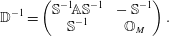 $$\begin{eqnarray}\mathbb{D}^{-1}=\left(\begin{array}{@{}cc@{}}\mathbb{S}^{-1}\!\mathbb{A}\mathbb{S}^{-1} & -\,\mathbb{S}^{-1}\\ \mathbb{S}^{-1} & \mathbb{O}_{M}\end{array}\right).\end{eqnarray}$$
Because of the block diagonal structure of (2.29), the Dirac bracket (2.21) becomes
 $$\begin{eqnarray}\{\,f,g\}_{\ast }=\{\,f,g\}+\mathbb{S}_{AB}^{-1}\left(\{\,f,C^{A}\}\{{\dot{C}}^{B},g\}-\{g,C^{A}\}\{{\dot{C}}^{B},f\}\right)+\mathbb{S}_{AC}^{-1}\,\mathbb{A}^{CD}\,\mathbb{S}_{DB}^{-1}\,\{\,f,C^{A}\}\{C^{B},g\},\end{eqnarray}$$
which has the form
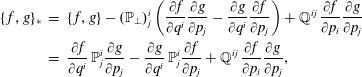 $$\begin{eqnarray}\displaystyle \{\,f,g\}_{\ast } & = & \displaystyle \{\,f,g\}-(\mathbb{P}_{\bot })_{j}^{i}\left(\frac{\unicode[STIX]{x2202}f}{\unicode[STIX]{x2202}q^{i}}\frac{\unicode[STIX]{x2202}g}{\unicode[STIX]{x2202}p_{j}}-\frac{\unicode[STIX]{x2202}g}{\unicode[STIX]{x2202}q^{i}}\frac{\unicode[STIX]{x2202}f}{\unicode[STIX]{x2202}p_{j}}\right)+\mathbb{Q}^{ij}\,\frac{\unicode[STIX]{x2202}f}{\unicode[STIX]{x2202}p_{i}}\frac{\unicode[STIX]{x2202}g}{\unicode[STIX]{x2202}p_{j}}\nonumber\\ \displaystyle & = & \displaystyle \frac{\unicode[STIX]{x2202}f}{\unicode[STIX]{x2202}q^{i}}\,\mathbb{P}_{j}^{i}\frac{\unicode[STIX]{x2202}g}{\unicode[STIX]{x2202}p_{j}}-\frac{\unicode[STIX]{x2202}g}{\unicode[STIX]{x2202}q^{i}}\,\mathbb{P}_{j}^{i}\frac{\unicode[STIX]{x2202}f}{\unicode[STIX]{x2202}p_{j}}+\mathbb{Q}^{ij}\,\frac{\unicode[STIX]{x2202}f}{\unicode[STIX]{x2202}p_{i}}\frac{\unicode[STIX]{x2202}g}{\unicode[STIX]{x2202}p_{j}},\end{eqnarray}$$
 where the matrices  $\mathbb{P}=\unicode[STIX]{x1D644}-\mathbb{P}_{\bot }$, with
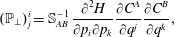 $$\begin{eqnarray}(\mathbb{P}_{\bot })_{j}^{i}=\mathbb{S}_{AB}^{-1}\,\frac{\unicode[STIX]{x2202}^{2}H}{\unicode[STIX]{x2202}p_{i}\unicode[STIX]{x2202}p_{k}}\frac{\unicode[STIX]{x2202}C^{A}}{\unicode[STIX]{x2202}q^{j}}\frac{\unicode[STIX]{x2202}C^{B}}{\unicode[STIX]{x2202}q^{k}},\end{eqnarray}$$
 and  $\mathbb{Q}$, a complicated expression that we will not record, are crafted using the constraints and Hamiltonian so as to make $\{\,f,g\}_{\ast }$ preserve the constraints.
The equations of motion that follow from (2.30) are
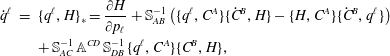 $$\begin{eqnarray}\displaystyle \dot{q}^{\ell } & = & \displaystyle \{q^{\ell },H\}_{\ast }=\frac{\unicode[STIX]{x2202}H}{\unicode[STIX]{x2202}p_{\ell }}+\mathbb{S}_{AB}^{-1}\left(\{q^{\ell },C^{A}\}\{{\dot{C}}^{B},H\}-\{H,C^{A}\}\{{\dot{C}}^{B},q^{\ell }\}\right)\nonumber\\ \displaystyle & & \displaystyle +\,\mathbb{S}_{AC}^{-1}\,\mathbb{A}^{CD}\,\mathbb{S}_{DB}^{-1}\,\{q^{\ell },C^{A}\}\{C^{B},H\},\end{eqnarray}$$
 $$\begin{eqnarray}\displaystyle {\dot{p}}_{\ell } & = & \displaystyle \{p_{\ell },H\}_{\ast }=-\frac{\unicode[STIX]{x2202}H}{\unicode[STIX]{x2202}q^{\ell }}+\mathbb{S}_{AB}^{-1}\left(\{p_{\ell },C^{A}\}\{{\dot{C}}^{B},H\}-\{H,C^{A}\}\{{\dot{C}}^{B},p_{\ell }\}\right)\nonumber\\ \displaystyle & & \displaystyle +\,\mathbb{S}_{AC}^{-1}\,\mathbb{A}^{CD}\,\mathbb{S}_{DB}^{-1}\,\{p_{\ell },C^{A}\}\{C^{B},H\}.\end{eqnarray}$$
 Given the Dirac bracket associated with the  $\mathbb{D}$ of (2.27), dynamics that enforces the constraints takes the form of (2.23). Any system generated by this bracket will enforce Lagrange’s holonomic constraints; however, only initial conditions compatible with
 $$\begin{eqnarray}D^{a}\equiv 0,\quad \forall a=M+1,M+2,\ldots ,2M,\end{eqnarray}$$
or equivalently
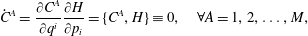 $$\begin{eqnarray}{\dot{C}}^{A}=\frac{\unicode[STIX]{x2202}C^{A}}{\unicode[STIX]{x2202}q^{i}}\frac{\unicode[STIX]{x2202}H}{\unicode[STIX]{x2202}p_{i}}=\{C^{A},H\}\equiv 0,\quad \forall A=1,2,\ldots ,M,\end{eqnarray}$$
 will correspond to the system with holonomic constraints. Using (2.36) and  $\{q^{\ell },C^{A}\}\equiv 0$, equations (2.33) and (2.34) reduce to
 $$\begin{eqnarray}\displaystyle & \displaystyle \dot{q}^{\ell }=\{q^{\ell },H\}_{\ast }=\frac{\unicode[STIX]{x2202}H}{\unicode[STIX]{x2202}p_{\ell }}, & \displaystyle\end{eqnarray}$$
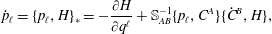 $$\begin{eqnarray}\displaystyle & \displaystyle {\dot{p}}_{\ell }=\{p_{\ell },H\}_{\ast }=-\frac{\unicode[STIX]{x2202}H}{\unicode[STIX]{x2202}q^{\ell }}+\mathbb{S}_{AB}^{-1}\{p_{\ell },C^{A}\}\{{\dot{C}}^{B},H\}, & \displaystyle\end{eqnarray}$$
where
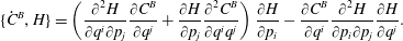 $$\begin{eqnarray}\{{\dot{C}}^{B},H\}=\left(\frac{\unicode[STIX]{x2202}^{2}H}{\unicode[STIX]{x2202}q^{i}\unicode[STIX]{x2202}p_{j}}\frac{\unicode[STIX]{x2202}C^{B}}{\unicode[STIX]{x2202}q^{j}}+\frac{\unicode[STIX]{x2202}H}{\unicode[STIX]{x2202}p_{j}}\frac{\unicode[STIX]{x2202}^{2}C^{B}}{\unicode[STIX]{x2202}q^{i}q^{j}}\right)\frac{\unicode[STIX]{x2202}H}{\unicode[STIX]{x2202}p_{i}}-\frac{\unicode[STIX]{x2202}C^{B}}{\unicode[STIX]{x2202}q^{i}}\frac{\unicode[STIX]{x2202}^{2}H}{\unicode[STIX]{x2202}p_{i}\unicode[STIX]{x2202}p_{j}}\frac{\unicode[STIX]{x2202}H}{\unicode[STIX]{x2202}q^{j}}.\end{eqnarray}$$
 Thus the Dirac bracket approach gives a relatively simple system for enforcing holonomic constraints. It can be shown directly that if initially  ${\dot{C}}^{A}$ vanishes, then the system of (2.37) and (2.38) will keep it so for all time.
2.3.1 Holonomic constraints and geodesic flow via Dirac
Let us now consider again the geodesic flow problem of § 2.1.1: the  $N$ degree-of-freedom free particle system with holonomic constraints, but this time within the framework of Dirac bracket theory. For this problem the unconstrained configuration space is the Euclidean space $\mathbb{E}^{3N}$ and we will denote by ${\mathcal{Q}}$ the constraint manifold within $\mathbb{E}^{3N}$ defined by the constancy of the constraints $C^{A}$.
The Lagrangian of (2.6) is easily Legendre transformed to the free particle Hamiltonian
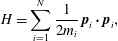 $$\begin{eqnarray}H=\mathop{\sum }_{i=1}^{N}\frac{1}{2m_{i}}\,\boldsymbol{p}_{i}\boldsymbol{\cdot }\boldsymbol{p}_{i},\end{eqnarray}$$
 where  $\boldsymbol{p}_{i}=m_{i}\dot{\boldsymbol{q}}_{i}$. For this example the constraints of (2.25) take the form
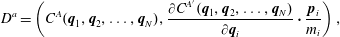 $$\begin{eqnarray}D^{a}=\left(C^{A}(\boldsymbol{q}_{1},\boldsymbol{q}_{2},\ldots ,\boldsymbol{q}_{N}),\frac{\unicode[STIX]{x2202}C^{A^{\prime }}(\boldsymbol{q}_{1},\boldsymbol{q}_{2},\ldots ,\boldsymbol{q}_{N})}{\unicode[STIX]{x2202}\boldsymbol{q}_{i}}\boldsymbol{\cdot }\frac{\boldsymbol{p}_{i}}{m_{i}}\right),\end{eqnarray}$$
 the  $M\times M$ matrix $\mathbb{S}$ has elements
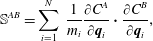 $$\begin{eqnarray}\mathbb{S}^{AB}=\mathop{\sum }_{i=1}^{N}\,\frac{1}{m_{i}}\frac{\unicode[STIX]{x2202}C^{A}}{\unicode[STIX]{x2202}\boldsymbol{q}_{i}}\boldsymbol{\cdot }\frac{\unicode[STIX]{x2202}C^{B}}{\unicode[STIX]{x2202}\boldsymbol{q}_{i}},\end{eqnarray}$$
 and the  $M\times M$ matrix $\mathbb{A}$ is
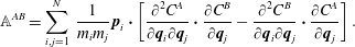 $$\begin{eqnarray}\mathbb{A}^{AB}=\mathop{\sum }_{i,j=1}^{N}\,\frac{1}{m_{i}m_{j}}\,\boldsymbol{p}_{i}\boldsymbol{\cdot }\left[\frac{\unicode[STIX]{x2202}^{2}C^{A}}{\unicode[STIX]{x2202}\boldsymbol{q}_{i}\unicode[STIX]{x2202}\boldsymbol{q}_{j}}\boldsymbol{\cdot }\frac{\unicode[STIX]{x2202}C^{B}}{\unicode[STIX]{x2202}\boldsymbol{q}_{j}}-\frac{\unicode[STIX]{x2202}^{2}C^{B}}{\unicode[STIX]{x2202}\boldsymbol{q}_{i}\unicode[STIX]{x2202}\boldsymbol{q}_{j}}\boldsymbol{\cdot }\frac{\unicode[STIX]{x2202}C^{A}}{\unicode[STIX]{x2202}\boldsymbol{q}_{j}}\right].\end{eqnarray}$$
The Dirac bracket analogous to (2.31) is
 $$\begin{eqnarray}\{\,f,g\}_{\ast }=\mathop{\sum }_{ij=1}^{N}\,\left[\frac{\unicode[STIX]{x2202}f}{\unicode[STIX]{x2202}\boldsymbol{q}_{i}}\boldsymbol{\cdot }\overset{\leftrightarrow }{\mathbb{P}}_{ij}\boldsymbol{\cdot }\frac{\unicode[STIX]{x2202}g}{\unicode[STIX]{x2202}\boldsymbol{p}_{j}}-\frac{\unicode[STIX]{x2202}g}{\unicode[STIX]{x2202}\boldsymbol{q}_{i}}\boldsymbol{\cdot }\overset{\leftrightarrow }{\mathbb{P}}_{ij}\boldsymbol{\cdot }\frac{\unicode[STIX]{x2202}f}{\unicode[STIX]{x2202}\boldsymbol{p}_{j}}+\frac{\unicode[STIX]{x2202}f}{\unicode[STIX]{x2202}\boldsymbol{p}_{i}}\boldsymbol{\cdot }\overset{\leftrightarrow }{\mathbb{Q}}_{ij}\boldsymbol{\cdot }\frac{\unicode[STIX]{x2202}g}{\unicode[STIX]{x2202}\boldsymbol{p}_{j}}\right],\end{eqnarray}$$
 where  $\overset{\leftrightarrow }{\mathbb{P}}_{ij}=\overset{\leftrightarrow }{\mathbb{I}}_{ij}-\overset{\leftrightarrow }{\mathbb{P}}_{\bot \,ij}$ with the tensors
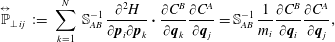 $$\begin{eqnarray}\displaystyle \overset{\leftrightarrow }{\mathbb{P}}_{\bot \,ij} & := & \displaystyle \mathop{\sum }_{k=1}^{N}\,\mathbb{S}_{AB}^{-1}\,\frac{\unicode[STIX]{x2202}^{2}H}{\unicode[STIX]{x2202}\boldsymbol{p}_{i}\unicode[STIX]{x2202}\boldsymbol{p}_{k}}\boldsymbol{\cdot }\frac{\unicode[STIX]{x2202}C^{B}}{\unicode[STIX]{x2202}\boldsymbol{q}_{k}}\frac{\unicode[STIX]{x2202}C^{A}}{\unicode[STIX]{x2202}\boldsymbol{q}_{j}}=\mathbb{S}_{AB}^{-1}\,\frac{1}{m_{i}}\frac{\unicode[STIX]{x2202}C^{B}}{\unicode[STIX]{x2202}\boldsymbol{q}_{i}}\frac{\unicode[STIX]{x2202}C^{A}}{\unicode[STIX]{x2202}\boldsymbol{q}_{j}},\end{eqnarray}$$
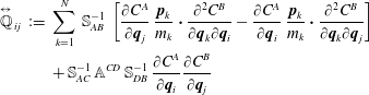 $$\begin{eqnarray}\displaystyle \overset{\leftrightarrow }{\mathbb{Q}}_{\,ij} & := & \displaystyle \mathop{\sum }_{k=1}^{N}\,\mathbb{S}_{AB}^{-1}\,\left[\frac{\unicode[STIX]{x2202}C^{A}}{\unicode[STIX]{x2202}\boldsymbol{q}_{j}}\,\frac{\boldsymbol{p}_{k}}{m_{k}}\boldsymbol{\cdot }\frac{\unicode[STIX]{x2202}^{2}C^{B}}{\unicode[STIX]{x2202}\boldsymbol{q}_{k}\unicode[STIX]{x2202}\boldsymbol{q}_{i}}-\frac{\unicode[STIX]{x2202}C^{A}}{\unicode[STIX]{x2202}\boldsymbol{q}_{i}}\,\frac{\boldsymbol{p}_{k}}{m_{k}}\boldsymbol{\cdot }\frac{\unicode[STIX]{x2202}^{2}C^{B}}{\unicode[STIX]{x2202}\boldsymbol{q}_{k}\unicode[STIX]{x2202}\boldsymbol{q}_{j}}\right]\nonumber\\ \displaystyle & & \displaystyle +\,\mathbb{S}_{AC}^{-1}\,\mathbb{A}^{CD}\,\mathbb{S}_{DB}^{-1}\,\frac{\unicode[STIX]{x2202}C^{A}}{\unicode[STIX]{x2202}\boldsymbol{q}_{i}}\frac{\unicode[STIX]{x2202}C^{B}}{\unicode[STIX]{x2202}\boldsymbol{q}_{j}}\end{eqnarray}$$
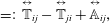 $$\begin{eqnarray}\displaystyle & =: & \displaystyle \overset{\leftrightarrow }{\mathbb{T}}_{ij}-\overset{\leftrightarrow }{\mathbb{T}}_{ji}+\overset{\leftrightarrow }{\mathbb{A}}_{ij},\end{eqnarray}$$
 where  $\overset{\leftrightarrow }{\mathbb{A}}_{ij}$ is the term with $\mathbb{S}_{AC}^{-1}\mathbb{A}^{CD}\mathbb{S}_{DB}^{-1}$. Observe $\overset{\leftrightarrow }{\mathbb{A}}_{ij}=-\overset{\leftrightarrow }{\mathbb{A}}_{ji}$ because $\mathbb{A}^{CD}=-\mathbb{A}^{DC}$ and
 $$\begin{eqnarray}\displaystyle \mathop{\sum }_{k=1}^{N}\,\overset{\leftrightarrow }{\mathbb{P}}_{\bot \,ik}\boldsymbol{\cdot }\overset{\leftrightarrow }{\mathbb{P}}_{\bot \,kj} & = & \displaystyle \mathop{\sum }_{k=1}^{N}\,\left(\mathbb{S}_{AB}^{-1}\,\frac{1}{m_{i}}\frac{\unicode[STIX]{x2202}C^{B}}{\unicode[STIX]{x2202}\boldsymbol{q}_{i}}\frac{\unicode[STIX]{x2202}C^{A}}{\unicode[STIX]{x2202}\boldsymbol{q}_{k}}\right)\boldsymbol{\cdot }\left(\mathbb{S}_{A^{\prime }B^{\prime }}^{-1}\,\frac{1}{m_{k}}\frac{\unicode[STIX]{x2202}C^{B^{\prime }}}{\unicode[STIX]{x2202}\boldsymbol{q}_{k}}\frac{\unicode[STIX]{x2202}C^{A^{\prime }}}{\unicode[STIX]{x2202}\boldsymbol{q}_{j}}\right)\nonumber\\ \displaystyle & = & \displaystyle \left(\mathbb{S}_{AB}^{-1}\,\frac{1}{m_{i}}\frac{\unicode[STIX]{x2202}C^{B}}{\unicode[STIX]{x2202}\boldsymbol{q}_{i}}\right)\mathbb{S}_{A^{\prime }B^{\prime }}^{-1}\,\left(\mathop{\sum }_{k=1}^{N}\,\frac{\unicode[STIX]{x2202}C^{A}}{\unicode[STIX]{x2202}\boldsymbol{q}_{k}}\boldsymbol{\cdot }\frac{1}{m_{k}}\frac{\unicode[STIX]{x2202}C^{B^{\prime }}}{\unicode[STIX]{x2202}\boldsymbol{q}_{k}}\right)\frac{\unicode[STIX]{x2202}C^{A^{\prime }}}{\unicode[STIX]{x2202}\boldsymbol{q}_{j}}\nonumber\\ \displaystyle & = & \displaystyle \left(\mathbb{S}_{AB}^{-1}\,\frac{1}{m_{i}}\frac{\unicode[STIX]{x2202}C^{B}}{\unicode[STIX]{x2202}\boldsymbol{q}_{i}}\right)\mathbb{S}_{A^{\prime }B^{\prime }}^{-1}\,\mathbb{S}^{AB^{\prime }}\frac{\unicode[STIX]{x2202}C^{A^{\prime }}}{\unicode[STIX]{x2202}\boldsymbol{q}_{j}}=\overset{\leftrightarrow }{\mathbb{P}}_{\bot \,ij}.\end{eqnarray}$$
Also observe for the Hamiltonian of (2.40)
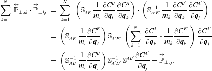
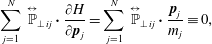 $$\begin{eqnarray}\displaystyle & \displaystyle \mathop{\sum }_{j=1}^{N}\,\overset{\leftrightarrow }{\mathbb{P}}_{\bot \,ij}\boldsymbol{\cdot }\frac{\unicode[STIX]{x2202}H}{\unicode[STIX]{x2202}\boldsymbol{p}_{j}}=\mathop{\sum }_{j=1}^{N}\,\overset{\leftrightarrow }{\mathbb{P}}_{\bot \,ij}\boldsymbol{\cdot }\frac{\boldsymbol{p}_{j}}{m_{j}}\equiv 0, & \displaystyle\end{eqnarray}$$
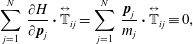 $$\begin{eqnarray}\displaystyle & \displaystyle \mathop{\sum }_{j=1}^{N}\,\frac{\unicode[STIX]{x2202}H}{\unicode[STIX]{x2202}\boldsymbol{p}_{j}}\boldsymbol{\cdot }\overset{\leftrightarrow }{\mathbb{T}}_{ij}=\mathop{\sum }_{j=1}^{N}\,\frac{\boldsymbol{p}_{j}}{m_{j}}\boldsymbol{\cdot }\overset{\leftrightarrow }{\mathbb{T}}_{ij}\equiv 0, & \displaystyle\end{eqnarray}$$
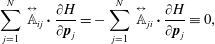 $$\begin{eqnarray}\displaystyle & \displaystyle \mathop{\sum }_{j=1}^{N}\,\overset{\leftrightarrow }{\mathbb{A}}_{ij}\boldsymbol{\cdot }\frac{\unicode[STIX]{x2202}H}{\unicode[STIX]{x2202}\boldsymbol{p}_{j}}=-\mathop{\sum }_{j=1}^{N}\,\overset{\leftrightarrow }{\mathbb{A}}_{ji}\boldsymbol{\cdot }\frac{\unicode[STIX]{x2202}H}{\unicode[STIX]{x2202}\boldsymbol{p}_{j}}\equiv 0, & \displaystyle\end{eqnarray}$$
 when evaluated on the constraint  ${\dot{C}}^{A,B}=0$, while
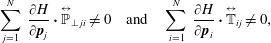 $$\begin{eqnarray}\mathop{\sum }_{j=1}^{N}\,\frac{\unicode[STIX]{x2202}H}{\unicode[STIX]{x2202}\boldsymbol{p}_{j}}\boldsymbol{\cdot }\overset{\leftrightarrow }{\mathbb{P}}_{\bot \,ji}\neq 0\quad \text{and}\quad \mathop{\sum }_{i=1}^{N}\,\frac{\unicode[STIX]{x2202}H}{\unicode[STIX]{x2202}\boldsymbol{p}_{i}}\boldsymbol{\cdot }\overset{\leftrightarrow }{\mathbb{T}}_{ij}\neq 0,\end{eqnarray}$$
 when evaluated on the constraint  ${\dot{C}}^{A,B}=0$. Thus, the bracket of (2.44) yields the equations of motion
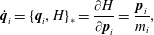 $$\begin{eqnarray}\displaystyle & \displaystyle \dot{\boldsymbol{q}}_{i}=\{\boldsymbol{q}_{i},H\}_{\ast }=\frac{\unicode[STIX]{x2202}H}{\unicode[STIX]{x2202}\boldsymbol{p}_{i}}=\frac{\boldsymbol{p}_{i}}{m_{i}}, & \displaystyle\end{eqnarray}$$
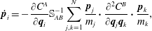 $$\begin{eqnarray}\displaystyle & \displaystyle \dot{\boldsymbol{p}}_{i}=-\frac{\unicode[STIX]{x2202}C^{A}}{\unicode[STIX]{x2202}\boldsymbol{q}_{i}}\mathbb{S}_{AB}^{-1}\mathop{\sum }_{j,k=1}^{N}\frac{\boldsymbol{p}_{j}}{m_{j}}\boldsymbol{\cdot }\frac{\unicode[STIX]{x2202}^{2}C^{B}}{\unicode[STIX]{x2202}\boldsymbol{q}_{j}\boldsymbol{q}_{k}}\boldsymbol{\cdot }\frac{\boldsymbol{p}_{k}}{m_{k}}, & \displaystyle\end{eqnarray}$$
or
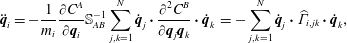 $$\begin{eqnarray}\ddot{\boldsymbol{q}}_{i}=-\frac{1}{m_{i}}\frac{\unicode[STIX]{x2202}C^{A}}{\unicode[STIX]{x2202}\boldsymbol{q}_{i}}\mathbb{S}_{AB}^{-1}\mathop{\sum }_{j,k=1}^{N}\dot{\boldsymbol{q}}_{j}\boldsymbol{\cdot }\frac{\unicode[STIX]{x2202}^{2}C^{B}}{\unicode[STIX]{x2202}\boldsymbol{q}_{j}\boldsymbol{q}_{k}}\boldsymbol{\cdot }\dot{\boldsymbol{q}}_{k}\,=-\mathop{\sum }_{j,k=1}^{N}\dot{\boldsymbol{q}}_{j}\boldsymbol{\cdot }\widehat{\unicode[STIX]{x1D6E4}}_{i,jk}\boldsymbol{\cdot }\dot{\boldsymbol{q}}_{k},\end{eqnarray}$$
where
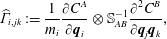 $$\begin{eqnarray}\widehat{\unicode[STIX]{x1D6E4}}_{i,jk}:=\frac{1}{m_{i}}\frac{\unicode[STIX]{x2202}C^{A}}{\unicode[STIX]{x2202}\boldsymbol{q}_{i}}\otimes \mathbb{S}_{AB}^{-1}\frac{\unicode[STIX]{x2202}^{2}C^{B}}{\unicode[STIX]{x2202}\boldsymbol{q}_{j}\boldsymbol{q}_{k}},\end{eqnarray}$$
is used to represent the normal force.
Observe, equation (2.55) has two essential features: as noted, its right-hand side is a normal force that projects to the constraint manifold defined by the constraints  $C^{A}$ and within the constraint manifold it describes a geodesic flow, all done in terms of the original Euclidean space coordinates where the initial conditions place the flow on ${\mathcal{Q}}$ by setting the values $C^{A}$ for all $A=1,2,\ldots ,M$. We will show this explicitly.
First, because the components of vectors normal to  ${\mathcal{Q}}$ are given by $\unicode[STIX]{x2202}C^{A}/\unicode[STIX]{x2202}\boldsymbol{q}_{i}$ for $A=1,2,\ldots ,M$, this prefactor on the righthand side of (2.55) projects as expected. Upon comparing (2.55) with (2.7) we conclude that the coefficient of this prefactor must be the Lagrange multipliers, i.e.
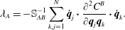 $$\begin{eqnarray}\unicode[STIX]{x1D706}_{A}=-\mathbb{S}_{AB}^{-1}\mathop{\sum }_{k,j=1}^{N}\dot{\boldsymbol{q}}_{j}\boldsymbol{\cdot }\frac{\unicode[STIX]{x2202}^{2}C^{B}}{\unicode[STIX]{x2202}\boldsymbol{q}_{j}\boldsymbol{q}_{k}}\boldsymbol{\cdot }\dot{\boldsymbol{q}}_{k}.\end{eqnarray}$$
Thus, we see that Dirac’s procedure explicitly solves for the Lagrange multiplier.
Second, to uncover the geodesic flow we can proceed as usual by projecting explicitly onto  ${\mathcal{Q}}$. To this end we consider the transformation between the Euclidean configuration space $\mathbb{E}^{3N}$ coordinates
 $$\begin{eqnarray}(\boldsymbol{q}_{1},\boldsymbol{q}_{2},\ldots ,\boldsymbol{q}_{i},\ldots ,\boldsymbol{q}_{N}),\quad \text{where }i=1,2,\ldots ,N\end{eqnarray}$$
and another set of coordinates
 $$\begin{eqnarray}(q^{1},q^{2},\ldots ,q^{a},\ldots ,q^{3N}),\quad \text{where }a=1,2,\ldots ,3N,\end{eqnarray}$$
which we tailor as follows:
 $$\begin{eqnarray}(q^{1},q^{2},\ldots ,q^{\unicode[STIX]{x1D6FC}}\ldots ,q^{n},C^{1},C^{2},\ldots ,C^{A},\ldots ,C^{M}),\end{eqnarray}$$
 where  $\unicode[STIX]{x1D6FC}=1,2,\ldots ,n$, $A=1,2,\ldots ,M$ and $n=3N-M$. Here we have chosen $q^{n+A}=C^{A}$ and $n$ is the actual number of degrees of freedom on the constraint surface ${\mathcal{Q}}$. We can freely transform back and forth between the two coordinates, i.e.
 $$\begin{eqnarray}(\boldsymbol{q}_{1},\boldsymbol{q}_{2},\ldots ,\boldsymbol{q}_{i},\ldots ,\boldsymbol{q}_{N})\longleftrightarrow (q^{1},q^{2},\ldots ,q^{a},\ldots ,q^{3N}).\end{eqnarray}$$
 Note, the choice  $q^{n+A}=C^{A}$ could be replaced by $q^{n+A}=f^{A}(C^{1},C^{2},\ldots ,C^{M})$ for arbitrary independent $f^{A}$, but we assume the original $C^{A}$ are optimal. Because $q^{\unicode[STIX]{x1D6FC}}$ are coordinates within ${\mathcal{Q}}$, tangent vectors to ${\mathcal{Q}}$ have the components $\unicode[STIX]{x2202}\boldsymbol{q}_{i}/\unicode[STIX]{x2202}q^{\unicode[STIX]{x1D6FC}}$, and there is one for each $\unicode[STIX]{x1D6FC}=1,2,\ldots ,n$. The pairing of the normals with tangents is expressed by
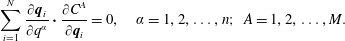 $$\begin{eqnarray}\mathop{\sum }_{i=1}^{N}\frac{\unicode[STIX]{x2202}\boldsymbol{q}_{i}}{\unicode[STIX]{x2202}q^{\unicode[STIX]{x1D6FC}}}\boldsymbol{\cdot }\frac{\unicode[STIX]{x2202}C^{A}}{\unicode[STIX]{x2202}\boldsymbol{q}_{i}}=0,\quad \unicode[STIX]{x1D6FC}=1,2,\ldots ,n;~A=1,2,\ldots ,M.\end{eqnarray}$$
Let us now consider an alternative procedure that the Dirac constraint method provides. Proceeding directly we calculate
 $$\begin{eqnarray}\dot{q}^{a}=\mathop{\sum }_{i=1}^{N}\frac{\unicode[STIX]{x2202}q^{a}}{\unicode[STIX]{x2202}\boldsymbol{q}_{i}}\boldsymbol{\cdot }\dot{\boldsymbol{q}}_{i}.\end{eqnarray}$$
 Observe that on  $\mathbb{E}^{3N}$ the matrix $\unicode[STIX]{x2202}q^{a}/\unicode[STIX]{x2202}\boldsymbol{q}_{i}$ is invertible and the full metric tensor and its inverse in the new coordinates are given as follows:
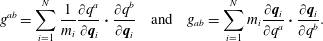 $$\begin{eqnarray}g^{ab}=\mathop{\sum }_{i=1}^{N}\frac{1}{m_{i}}\frac{\unicode[STIX]{x2202}q^{a}}{\unicode[STIX]{x2202}\boldsymbol{q}_{i}}\boldsymbol{\cdot }\frac{\unicode[STIX]{x2202}q^{b}}{\unicode[STIX]{x2202}\boldsymbol{q}_{i}}\quad \text{and}\quad g_{ab}=\mathop{\sum }_{i=1}^{N}m_{i}\frac{\unicode[STIX]{x2202}\boldsymbol{q}_{i}}{\unicode[STIX]{x2202}q^{a}}\boldsymbol{\cdot }\frac{\unicode[STIX]{x2202}\boldsymbol{q}_{i}}{\unicode[STIX]{x2202}q^{b}}.\end{eqnarray}$$
 The metric tensor on  ${\mathcal{Q}}$ of (2.9) is obtained by restricting $g_{ab}$ to $a,b\leqslant n$ and $g^{\unicode[STIX]{x1D6FC}\unicode[STIX]{x1D6FD}}$ is obtained by inverting $g_{\unicode[STIX]{x1D6FC}\unicode[STIX]{x1D6FD}}$ and not by restricting $g_{ab}$. Proceeding by differentiating again we obtain
 $$\begin{eqnarray}\ddot{q}^{a}=\mathop{\sum }_{i=1}^{N}\frac{\unicode[STIX]{x2202}q^{a}}{\unicode[STIX]{x2202}\boldsymbol{q}_{i}}\boldsymbol{\cdot }\ddot{\boldsymbol{q}}_{i}+\mathop{\sum }_{i,j=1}^{N}\dot{\boldsymbol{q}}_{i}\boldsymbol{\cdot }\frac{\unicode[STIX]{x2202}^{2}q^{a}}{\unicode[STIX]{x2202}\boldsymbol{q}_{i}\unicode[STIX]{x2202}\boldsymbol{q}_{j}}\boldsymbol{\cdot }\dot{\boldsymbol{q}}_{j},\quad a=1,2,\ldots ,3N.\end{eqnarray}$$
Now inserting (2.55) into (2.65) gives
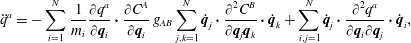 $$\begin{eqnarray}\ddot{q}^{a}=-\mathop{\sum }_{i=1}^{N}\frac{1}{m_{i}}\frac{\unicode[STIX]{x2202}q^{a}}{\unicode[STIX]{x2202}\boldsymbol{q}_{i}}\boldsymbol{\cdot }\frac{\unicode[STIX]{x2202}C^{A}}{\unicode[STIX]{x2202}\boldsymbol{q}_{i}}\,g_{AB}\mathop{\sum }_{j,k=1}^{N}\dot{\boldsymbol{q}}_{j}\boldsymbol{\cdot }\frac{\unicode[STIX]{x2202}^{2}C^{B}}{\unicode[STIX]{x2202}\boldsymbol{q}_{j}\boldsymbol{q}_{k}}\boldsymbol{\cdot }\dot{\boldsymbol{q}}_{k}+\mathop{\sum }_{i,j=1}^{N}\dot{\boldsymbol{q}}_{j}\boldsymbol{\cdot }\frac{\unicode[STIX]{x2202}^{2}q^{a}}{\unicode[STIX]{x2202}\boldsymbol{q}_{i}\unicode[STIX]{x2202}\boldsymbol{q}_{j}}\boldsymbol{\cdot }\dot{\boldsymbol{q}}_{i},\end{eqnarray}$$
where we have recognized that
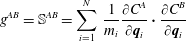 $$\begin{eqnarray}g^{AB}=\mathbb{S}^{AB}=\mathop{\sum }_{i=1}^{N}\,\frac{1}{m_{i}}\frac{\unicode[STIX]{x2202}C^{A}}{\unicode[STIX]{x2202}\boldsymbol{q}_{i}}\boldsymbol{\cdot }\frac{\unicode[STIX]{x2202}C^{B}}{\unicode[STIX]{x2202}\boldsymbol{q}_{i}}\end{eqnarray}$$
 and, as was necessary for the workability of the Dirac bracket constraint theory,  $g_{AB}=\mathbb{S}_{AB}^{-1}$ must exist. This quantity is obtained by inverting $\mathbb{S}^{AB}$ and not by restricting $g^{ab}$.
Equation (2.66) is an expression for the full system on  $\mathbb{E}^{3N}$. However, for $a>n$, we know $\ddot{q}^{a}=\ddot{C}^{A}=0$, so the two terms of (2.66) should cancel. To see this, in the first term of (2.66) we set $q^{a}=C^{C}$ and observe that this first term becomes
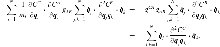 $$\begin{eqnarray}\displaystyle -\mathop{\sum }_{i=1}^{N}\frac{1}{m_{i}}\frac{\unicode[STIX]{x2202}C^{C}}{\unicode[STIX]{x2202}\boldsymbol{q}_{i}}\boldsymbol{\cdot }\frac{\unicode[STIX]{x2202}C^{A}}{\unicode[STIX]{x2202}\boldsymbol{q}_{i}}\,g_{AB}\mathop{\sum }_{j,k=1}^{N}\dot{\boldsymbol{q}}_{j}\boldsymbol{\cdot }\frac{\unicode[STIX]{x2202}^{2}C^{B}}{\unicode[STIX]{x2202}\boldsymbol{q}_{j}\boldsymbol{q}_{k}}\boldsymbol{\cdot }\dot{\boldsymbol{q}}_{k} & = & \displaystyle -g^{CA}\,g_{AB}\mathop{\sum }_{j,k=1}^{N}\dot{\boldsymbol{q}}_{j}\boldsymbol{\cdot }\frac{\unicode[STIX]{x2202}^{2}C^{B}}{\unicode[STIX]{x2202}\boldsymbol{q}_{j}\boldsymbol{q}_{k}}\boldsymbol{\cdot }\dot{\boldsymbol{q}}_{k}\nonumber\\ \displaystyle & = & \displaystyle -\mathop{\sum }_{j,k=1}^{N}\dot{\boldsymbol{q}}_{j}\boldsymbol{\cdot }\frac{\unicode[STIX]{x2202}^{2}C^{C}}{\unicode[STIX]{x2202}\boldsymbol{q}_{j}\boldsymbol{q}_{k}}\boldsymbol{\cdot }\dot{\boldsymbol{q}}_{k}.\end{eqnarray}$$
 Now, for  $a\leqslant n$, say $\unicode[STIX]{x1D6FC}$, the right-hand side gives a Christoffel symbol expression for the geodesic flow; viz.
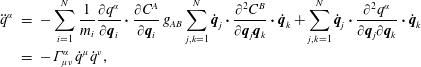 $$\begin{eqnarray}\displaystyle \ddot{q}^{\unicode[STIX]{x1D6FC}} & = & \displaystyle -\mathop{\sum }_{i=1}^{N}\frac{1}{m_{i}}\frac{\unicode[STIX]{x2202}q^{\unicode[STIX]{x1D6FC}}}{\unicode[STIX]{x2202}\boldsymbol{q}_{i}}\boldsymbol{\cdot }\frac{\unicode[STIX]{x2202}C^{A}}{\unicode[STIX]{x2202}\boldsymbol{q}_{i}}\,g_{AB}\mathop{\sum }_{j,k=1}^{N}\dot{\boldsymbol{q}}_{j}\boldsymbol{\cdot }\frac{\unicode[STIX]{x2202}^{2}C^{B}}{\unicode[STIX]{x2202}\boldsymbol{q}_{j}\boldsymbol{q}_{k}}\boldsymbol{\cdot }\dot{\boldsymbol{q}}_{k}+\mathop{\sum }_{j,k=1}^{N}\dot{\boldsymbol{q}}_{j}\boldsymbol{\cdot }\frac{\unicode[STIX]{x2202}^{2}q^{\unicode[STIX]{x1D6FC}}}{\unicode[STIX]{x2202}\boldsymbol{q}_{j}\unicode[STIX]{x2202}\boldsymbol{q}_{k}}\boldsymbol{\cdot }\dot{\boldsymbol{q}}_{k}\nonumber\\ \displaystyle & = & \displaystyle -\unicode[STIX]{x1D6E4}_{\unicode[STIX]{x1D707}\unicode[STIX]{x1D708}}^{\unicode[STIX]{x1D6FC}}\,\dot{q}^{\unicode[STIX]{x1D707}}\dot{q}^{\unicode[STIX]{x1D708}},\end{eqnarray}$$
where
 $$\begin{eqnarray}\unicode[STIX]{x1D6E4}_{\unicode[STIX]{x1D707}\unicode[STIX]{x1D708}}^{\unicode[STIX]{x1D6FC}}=\mathop{\sum }_{i=1}^{N}\frac{1}{m_{i}}\frac{\unicode[STIX]{x2202}q^{\unicode[STIX]{x1D6FC}}}{\unicode[STIX]{x2202}\boldsymbol{q}_{i}}\boldsymbol{\cdot }\frac{\unicode[STIX]{x2202}C^{A}}{\unicode[STIX]{x2202}\boldsymbol{q}_{i}}\,\mathbb{S}_{AB}^{-1}\mathop{\sum }_{j,k=1}^{N}\frac{\unicode[STIX]{x2202}\boldsymbol{q}_{j}}{\unicode[STIX]{x2202}q^{\unicode[STIX]{x1D707}}}\boldsymbol{\cdot }\frac{\unicode[STIX]{x2202}^{2}C^{B}}{\unicode[STIX]{x2202}\boldsymbol{q}_{j}\boldsymbol{q}_{k}}\boldsymbol{\cdot }\frac{\unicode[STIX]{x2202}\boldsymbol{q}_{k}}{\unicode[STIX]{x2202}q^{\unicode[STIX]{x1D708}}}+\mathop{\sum }_{j,k=1}^{N}\frac{\unicode[STIX]{x2202}\boldsymbol{q}_{j}}{\unicode[STIX]{x2202}q^{\unicode[STIX]{x1D707}}}\boldsymbol{\cdot }\frac{\unicode[STIX]{x2202}^{2}q^{\unicode[STIX]{x1D6FC}}}{\unicode[STIX]{x2202}\boldsymbol{q}_{j}\unicode[STIX]{x2202}\boldsymbol{q}_{k}}\boldsymbol{\cdot }\frac{\unicode[STIX]{x2202}\boldsymbol{q}_{k}}{\unicode[STIX]{x2202}q^{\unicode[STIX]{x1D708}}}\end{eqnarray}$$
 is an expression for the Christoffel symbol in terms of the original Euclidean coordinates, the constraints and the choice of coordinates on  ${\mathcal{Q}}$.
Using (2.70) one can calculate an analogous expression for the Riemann curvature tensor on  ${\mathcal{Q}}$ from the usual expression
 $$\begin{eqnarray}R_{\unicode[STIX]{x1D6FD}\unicode[STIX]{x1D6FE}\unicode[STIX]{x1D6FF}}^{\unicode[STIX]{x1D6FC}}=\frac{\unicode[STIX]{x2202}\unicode[STIX]{x1D6E4}_{\unicode[STIX]{x1D6FF}\unicode[STIX]{x1D6FD}}^{\unicode[STIX]{x1D6FC}}}{\unicode[STIX]{x2202}q^{\unicode[STIX]{x1D6FE}}}-\frac{\unicode[STIX]{x2202}\unicode[STIX]{x1D6E4}_{\unicode[STIX]{x1D6FE}\unicode[STIX]{x1D6FD}}^{\unicode[STIX]{x1D6FC}}}{\unicode[STIX]{x2202}q^{\unicode[STIX]{x1D6FF}}}+\unicode[STIX]{x1D6E4}_{\unicode[STIX]{x1D6FE}\unicode[STIX]{x1D706}}^{\unicode[STIX]{x1D6FC}}\unicode[STIX]{x1D6E4}_{\unicode[STIX]{x1D6FF}\unicode[STIX]{x1D6FD}}^{\unicode[STIX]{x1D706}}-\unicode[STIX]{x1D6E4}_{\unicode[STIX]{x1D6FF}\unicode[STIX]{x1D706}}^{\unicode[STIX]{x1D6FC}}\unicode[STIX]{x1D6E4}_{\unicode[STIX]{x1D6FE}\unicode[STIX]{x1D6FD}}^{\unicode[STIX]{x1D706}},\end{eqnarray}$$
 using  $\unicode[STIX]{x2202}/\unicode[STIX]{x2202}q^{\unicode[STIX]{x1D6FE}}=\sum _{i}(\unicode[STIX]{x2202}\boldsymbol{q}_{i}/\unicode[STIX]{x2202}q^{\unicode[STIX]{x1D6FE}})\boldsymbol{\cdot }\unicode[STIX]{x2202}/\unicode[STIX]{x2202}\boldsymbol{q}_{i}$. This gives the curvature written in terms of the original Euclidean coordinates, the constraints, and the chosen coordinates on ${\mathcal{Q}}$.
2.4 The  $d+1$ field theory

The techniques of §§ 2.1–2.3 have natural extensions to field theory.
Given independent field variables  $\unicode[STIX]{x1D6F9}^{{\mathcal{A}}}(\unicode[STIX]{x1D707},t)$, indexed by ${\mathcal{A}}=1,2,\ldots ,\ell$, where the independent variable $\unicode[STIX]{x1D707}=(\unicode[STIX]{x1D707}^{1},\unicode[STIX]{x1D707}^{2},\ldots ,\unicode[STIX]{x1D707}^{d})$. The field theoretic version of Hamilton’s principle of (2.1) is embodied in the action
 $$\begin{eqnarray}S[\unicode[STIX]{x1D6F9}]=\int _{t_{0}}^{t_{1}}\,\text{d}t\,L[\unicode[STIX]{x1D6F9},\dot{\unicode[STIX]{x1D6F9}}],\quad \text{with }L[\unicode[STIX]{x1D6F9},\dot{\unicode[STIX]{x1D6F9}}]=\int \text{d}^{d}\!\unicode[STIX]{x1D707}\,{\mathcal{L}}(\unicode[STIX]{x1D6F9},\dot{\unicode[STIX]{x1D6F9}},\unicode[STIX]{x2202}\unicode[STIX]{x1D6F9}),\end{eqnarray}$$
 where we leave the domain of  $\unicode[STIX]{x1D707}$ and the boundary conditions unspecified, but freely drop surface terms obtained upon integration by parts. The Lagrangian density ${\mathcal{L}}$ is assumed to depend on the field components $\unicode[STIX]{x1D6F9}$ and $\unicode[STIX]{x2202}\unicode[STIX]{x1D6F9}$, which is used to indicate all possible partial derivatives with respect of the components of $\unicode[STIX]{x1D707}$. Hamilton’s principle with (2.72) gives the Euler–Lagrange equations,
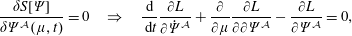 $$\begin{eqnarray}\frac{\unicode[STIX]{x1D6FF}S[\unicode[STIX]{x1D6F9}]}{\unicode[STIX]{x1D6FF}\unicode[STIX]{x1D6F9}^{{\mathcal{A}}}(\unicode[STIX]{x1D707},t)}=0\quad \Rightarrow \quad \frac{\text{d}}{\,\text{d}t}\frac{\unicode[STIX]{x2202}L}{\unicode[STIX]{x2202}\dot{\unicode[STIX]{x1D6F9}}^{{\mathcal{A}}}}+\frac{\unicode[STIX]{x2202}}{\unicode[STIX]{x2202}\unicode[STIX]{x1D707}}\frac{\unicode[STIX]{x2202}L}{\unicode[STIX]{x2202}\unicode[STIX]{x2202}\unicode[STIX]{x1D6F9}^{{\mathcal{A}}}}-\frac{\unicode[STIX]{x2202}L}{\unicode[STIX]{x2202}\unicode[STIX]{x1D6F9}^{{\mathcal{A}}}}=0,\end{eqnarray}$$
 where the overdot implies differentiation at constant  $\unicode[STIX]{x1D707}$. Local holonomic constraints $C^{A}(\unicode[STIX]{x1D6F9},\unicode[STIX]{x2202}\unicode[STIX]{x1D6F9})$ are enforced by Lagrange’s method by amending the Lagrangian
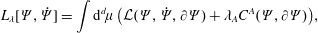 $$\begin{eqnarray}L_{\unicode[STIX]{x1D706}}[\unicode[STIX]{x1D6F9},\dot{\unicode[STIX]{x1D6F9}}]=\int \text{d}^{d}\!\unicode[STIX]{x1D707}\,\big({\mathcal{L}}(\unicode[STIX]{x1D6F9},\dot{\unicode[STIX]{x1D6F9}},\unicode[STIX]{x2202}\unicode[STIX]{x1D6F9})+\unicode[STIX]{x1D706}_{A}C^{A}(\unicode[STIX]{x1D6F9},\unicode[STIX]{x2202}\unicode[STIX]{x1D6F9})\big),\end{eqnarray}$$
 with again  $A=1,2,\ldots ,M$ and proceeding as in the finite-dimensional case.
In the Hamiltonian field theoretic setting, we could introduce the conjugate momentum densities  $\unicode[STIX]{x03C0}_{{\mathcal{A}}}$, ${\mathcal{A}}=1,2,\ldots ,\ell$, with the phase space action
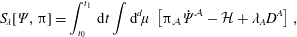 $$\begin{eqnarray}S_{\!\unicode[STIX]{x1D706}}[\unicode[STIX]{x1D6F9},\unicode[STIX]{x03C0}]=\int _{t_{0}}^{t_{1}}\,\text{d}t\int \text{d}^{d}\!\unicode[STIX]{x1D707}\,\left[\unicode[STIX]{x03C0}_{{\mathcal{A}}}\dot{\unicode[STIX]{x1D6F9}}^{{\mathcal{A}}}-{\mathcal{H}}+\unicode[STIX]{x1D706}_{A}D^{A}\right],\end{eqnarray}$$
 with Hamiltonian density  ${\mathcal{H}}$ and local constraints $D^{a}$ depending on the values of the fields and their conjugates. Instead of following this route we will jump directly to a generalization of the field theoretic Dirac bracket formalism that would result.
Consider a Poisson algebra composed of functionals of field variables  $\unicode[STIX]{x1D712}^{{\mathcal{A}}}(\unicode[STIX]{x1D707},t)$ with a Poisson bracket of the form
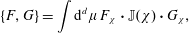 $$\begin{eqnarray}\{F,G\}=\int \text{d}^{d}\unicode[STIX]{x1D707}\,F_{\unicode[STIX]{x1D712}}\boldsymbol{\cdot }\mathbb{J}(\unicode[STIX]{x1D712})\boldsymbol{\cdot }G_{\unicode[STIX]{x1D712}},\end{eqnarray}$$
 where  $F_{\unicode[STIX]{x1D712}}$ is a shorthand for the functional derivative of a functional $F$ with respect to the field $\unicode[STIX]{x1D712}$ (see e.g. Morrison (Reference Morrison1998)) and $F_{\unicode[STIX]{x1D712}}\boldsymbol{\cdot }\mathbb{J}\boldsymbol{\cdot }G_{\unicode[STIX]{x1D712}}=F_{\unicode[STIX]{x1D712}^{{\mathcal{A}}}}\,\mathbb{J}^{{\mathcal{A}}{\mathcal{B}}}\,G_{\unicode[STIX]{x1D712}^{{\mathcal{B}}}}$, again with repeated indices summed. Observe the fields $\unicode[STIX]{x1D712}^{{\mathcal{A}}}(\unicode[STIX]{x1D707},t)$ need not separate into coordinates and momenta, but if they do the Poisson operator $\mathbb{J}$ has a form akin to that of (2.16). By a Poisson algebra we mean a Lie algebra realization on functionals, meaning the Poisson bracket is bilinear, antisymmetric, and satisfies the Jacobi identity and that there is an associative product of functionals that satisfies the Leibniz law. From the Poisson bracket the equations of motion are given by $\dot{\unicode[STIX]{x1D712}}=\{\unicode[STIX]{x1D712},H\}$, for some Hamiltonian functional $H[\unicode[STIX]{x1D712}]$.
Dirac’s constraint theory is generally implemented in terms of canonical Poisson brackets (see e.g. Dirac (Reference Dirac1950), Sudarshan & Makunda (Reference Sudarshan and Makunda1974), Sundermeyer (Reference Sundermeyer1982)), but it is not difficult to show that his procedure also works for noncanonical Poisson brackets (see e.g. an appendix of Morrison et al. Reference Morrison, Lebovitz and Biello2009).
We impose an even number of local constraints which we write as  $D^{a}(\unicode[STIX]{x1D707})=\text{const}.$, a shorthand for $D^{a}[\unicode[STIX]{x1D712}(\unicode[STIX]{x1D707})]$, with the index $a=1,2,\ldots ,2M$, bearing in mind that they depend on the fields $\unicode[STIX]{x1D712}$ and their derivatives. As in the finite-dimensional case, the Dirac bracket is obtained from the matrix $\mathbb{D}$ obtained from the bracket of the constraints,
 $$\begin{eqnarray}\mathbb{D}^{ab}(\unicode[STIX]{x1D707},\unicode[STIX]{x1D707}^{\prime })=\{D^{a}(\unicode[STIX]{x1D707}),D^{b}(\unicode[STIX]{x1D707}^{\prime })\},\end{eqnarray}$$
 where we note that  $\mathbb{D}^{ab}(\unicode[STIX]{x1D707},\unicode[STIX]{x1D707}^{\prime })=-\mathbb{D}^{ba}(\unicode[STIX]{x1D707}^{\prime },\unicode[STIX]{x1D707})$. If $\mathbb{D}$ has an inverse, then the Dirac bracket is defined as follows:
 $$\begin{eqnarray}\{F,G\}_{\ast }=\{F,G\}-\int \!\!\text{d}^{d}\unicode[STIX]{x1D707}\!\!\int \!\!\text{d}^{d}\unicode[STIX]{x1D707}^{\prime }\,\{F,D^{a}(\unicode[STIX]{x1D707})\}\mathbb{D}_{ab}^{-1}(\unicode[STIX]{x1D707},\unicode[STIX]{x1D707}^{\prime })\{D^{b}(\unicode[STIX]{x1D707}^{\prime }),G\},\end{eqnarray}$$
 where the coefficients  $\mathbb{D}_{ab}^{-1}(\unicode[STIX]{x1D707},\unicode[STIX]{x1D707}^{\prime })$ satisfy
 $$\begin{eqnarray}\int \!\!\text{d}^{d}\unicode[STIX]{x1D707}^{\prime }\,\mathbb{D}_{ab}^{-1}(\unicode[STIX]{x1D707},\unicode[STIX]{x1D707}^{\prime })\mathbb{D}^{bc}(\unicode[STIX]{x1D707}^{\prime },\unicode[STIX]{x1D707}^{\prime \prime })=\int \!\!\text{d}^{3}\unicode[STIX]{x1D707}^{\prime }\,\mathbb{D}^{cb}(\unicode[STIX]{x1D707},\unicode[STIX]{x1D707}^{\prime })\mathbb{D}_{ba}^{-1}(\unicode[STIX]{x1D707}^{\prime },\unicode[STIX]{x1D707}^{\prime \prime })=\unicode[STIX]{x1D6FF}_{a}^{c}\unicode[STIX]{x1D6FF}(\unicode[STIX]{x1D707}-\unicode[STIX]{x1D707}^{\prime \prime }),\end{eqnarray}$$
 consistent with  $\mathbb{D}_{ab}^{-1}(\unicode[STIX]{x1D707},\unicode[STIX]{x1D707}^{\prime })=-\mathbb{D}_{ba}^{-1}(\unicode[STIX]{x1D707}^{\prime },\unicode[STIX]{x1D707})$.
We note, the procedure is effective only when the coefficients  $\mathbb{D}_{ab}^{-1}(\unicode[STIX]{x1D707},\unicode[STIX]{x1D707}^{\prime })$ can be found. If $\mathbb{D}$ is not invertible, then one needs, in general, secondary constraints to determine the Dirac bracket.
2.4.1 Field theoretic geodesic flow
In light of § 2.1.1, any field theory with a Lagrangian density of the form
 $$\begin{eqnarray}{\mathcal{L}}={\textstyle \frac{1}{2}}\dot{\unicode[STIX]{x1D6F9}}^{{\mathcal{A}}}(\unicode[STIX]{x1D707},t)\,\unicode[STIX]{x1D702}_{{\mathcal{A}}{\mathcal{B}}}\,\dot{\unicode[STIX]{x1D6F9}}^{{\mathcal{B}}}(\unicode[STIX]{x1D707},t),\end{eqnarray}$$
 with the metric  $\unicode[STIX]{x1D702}_{{\mathcal{A}}{\mathcal{B}}}=\unicode[STIX]{x1D6FF}_{{\mathcal{A}}{\mathcal{B}}}$ being the Kronecker delta, subject to time-independent holonomic constraints can be viewed as geodesic flow on the constraint surface. This is a natural infinite-dimensional generalization of the idea of § 2.1.1.
3 Unconstrained Hamiltonian and action for fluid
3.1 Fluid action in Lagrangian variable description
The Lagrangian variable description of a fluid is described in Lagrange’s famous work (Lagrange Reference Lagrange1788), while historic and additional material can be found in Serrin (Reference Serrin and Flügge1959), Newcomb (Reference Newcomb1962), Van Kampen & Felderhof (Reference Van Kampen and Felderhof1967) and Morrison (Reference Morrison1998). Because the Lagrangian description treats a fluid as a continuum of particles, it naturally is amenable to the Hamiltonian form. The Lagrangian variable is a coordinate that gives the position of a fluid element or parcel, as it is sometimes called, at time  $t$. We denote this variable by $\boldsymbol{q}=\boldsymbol{q}(\boldsymbol{a},t)=(q^{1},q^{2},q^{3})$, which is measured relative to some cartesian coordinate system. Here $\boldsymbol{a}=(a^{1},a^{2},a^{3})$ denotes the fluid element label, which is often defined to be the position of the fluid element at the initial time, $\boldsymbol{a}=\boldsymbol{q}(\boldsymbol{a},0)$, but this need not always be the case. The label $\boldsymbol{a}$ is a continuum analogue of the discrete index that labels a generalized coordinate in a finite degree-of-freedom system. If $D$ is a domain that is fully occupied by the fluid, then at each fixed time $t$,
$t$,  $\boldsymbol{q}:D\rightarrow D$ is assumed to be 1–1 and onto. Not much is really known about the mathematical properties of this function, but we will assume that it is as smooth as it needs to be for the operations performed. Also, we will assume we can freely integrate by parts dropping surface terms and drop reference to $D$ in our integrals.
When discussing the ideal fluid and MHD we will use repeated sum notation with upper and lower indices even though we are working in cartesian coordinates. And, unlike in § 2, Latin indices,  $i,j,k,\ell$ etc. will be summed over 1,2 and 3, the cartesian components, rather than to $N$. This is done to avoid further proliferation of indices and we trust confusion will not arise because of context.
Important quantities are the deformation matrix,  $\unicode[STIX]{x2202}q^{i}/\unicode[STIX]{x2202}a^{j}$ and its Jacobian determinant ${\mathcal{J}}:=\det (\unicode[STIX]{x2202}q^{i}/\unicode[STIX]{x2202}a^{j})$, which is given by
 $$\begin{eqnarray}{\mathcal{J}}=\frac{1}{6}\unicode[STIX]{x1D716}_{kj\ell }\unicode[STIX]{x1D716}^{imn}\frac{\unicode[STIX]{x2202}q^{k}}{\unicode[STIX]{x2202}a^{i}}\frac{\unicode[STIX]{x2202}q^{j}}{\unicode[STIX]{x2202}a^{m}}\frac{\unicode[STIX]{x2202}q^{\ell }}{\unicode[STIX]{x2202}a^{n}},\end{eqnarray}$$
 where  $\unicode[STIX]{x1D716}_{ijk}=\unicode[STIX]{x1D716}^{ijk}$ is the purely antisymmetric (Levi–Civita) tensor density. We assume a fluid element is uniquely determined by its label for all time. Thus, ${\mathcal{J}}\neq 0$ and we can invert $\boldsymbol{q}=\boldsymbol{q}(\boldsymbol{a},t)$ to obtain the label associated with the fluid element at position $\boldsymbol{x}$ at time $t$,
$t$,  $\boldsymbol{a}=\boldsymbol{q}^{-1}(\boldsymbol{x},t)$. For coordinate transformations $\boldsymbol{q}=\boldsymbol{q}(\boldsymbol{a},t)$ we have
 $$\begin{eqnarray}\frac{\unicode[STIX]{x2202}q^{k}}{\unicode[STIX]{x2202}a^{j}}\,\frac{A_{k}^{i}}{{\mathcal{J}}}=\unicode[STIX]{x1D6FF}_{j}^{i},\end{eqnarray}$$
 where  $A_{k}^{i}$ is the cofactor of $\unicode[STIX]{x2202}q^{k}/\unicode[STIX]{x2202}a^{i}$, which can be written as follows:
 $$\begin{eqnarray}A_{k}^{i}=\frac{1}{2}\unicode[STIX]{x1D716}_{kj\ell }\unicode[STIX]{x1D716}^{imn}\frac{\unicode[STIX]{x2202}q^{j}}{\unicode[STIX]{x2202}a^{m}}\frac{\unicode[STIX]{x2202}q^{\ell }}{\unicode[STIX]{x2202}a^{n}}.\end{eqnarray}$$
 Using  $\boldsymbol{q}(\boldsymbol{a},t)$ or its inverse $\boldsymbol{q}^{-1}(\boldsymbol{x},t)$, various quantities can be written either as a function of $\boldsymbol{x}$ or $\boldsymbol{a}$. For convenience we list additional formulas below for latter use:
 $$\begin{eqnarray}\displaystyle & \displaystyle {\mathcal{J}}=\frac{1}{3}A_{\ell }^{k}\frac{\unicode[STIX]{x2202}q^{\ell }}{\unicode[STIX]{x2202}a^{k}}, & \displaystyle\end{eqnarray}$$
 $$\begin{eqnarray}\displaystyle & \displaystyle A_{i}^{j}=\frac{\unicode[STIX]{x2202}{\mathcal{J}}}{\unicode[STIX]{x2202}(\unicode[STIX]{x2202}q^{i}/\unicode[STIX]{x2202}a^{j})}, & \displaystyle\end{eqnarray}$$
 $$\begin{eqnarray}\displaystyle & \displaystyle \frac{\unicode[STIX]{x2202}(A_{i}^{k}f)}{\unicode[STIX]{x2202}a^{k}}=A_{i}^{k}\,\frac{\unicode[STIX]{x2202}f}{\unicode[STIX]{x2202}a^{k}}, & \displaystyle\end{eqnarray}$$
 $$\begin{eqnarray}\unicode[STIX]{x1D6FF}{\mathcal{J}}=A_{i}^{k}\frac{\unicode[STIX]{x2202}\unicode[STIX]{x1D6FF}q^{i}}{\unicode[STIX]{x2202}a^{k}}\quad \text{or}\quad \dot{{\mathcal{J}}}=A_{i}^{k}\frac{\unicode[STIX]{x2202}\dot{q}^{i}}{\unicode[STIX]{x2202}a^{k}},\end{eqnarray}$$
 $$\begin{eqnarray}\unicode[STIX]{x1D6FF}\left(\frac{A_{\ell }^{k}}{{\mathcal{J}}}\right)\frac{\unicode[STIX]{x2202}q^{\ell }}{\unicode[STIX]{x2202}a^{u}}=-\frac{A_{i}^{k}}{{\mathcal{J}}}\frac{\unicode[STIX]{x2202}}{\unicode[STIX]{x2202}a^{u}}\unicode[STIX]{x1D6FF}q^{i}\quad \text{or}\quad \unicode[STIX]{x1D6FF}\left(\frac{A_{\ell }^{k}}{{\mathcal{J}}}\right)=-\frac{A_{i}^{k}A_{\ell }^{u}}{{\mathcal{J}}^{2}}\frac{\unicode[STIX]{x2202}}{\unicode[STIX]{x2202}a^{u}}\unicode[STIX]{x1D6FF}q^{i},\end{eqnarray}$$
 $$\begin{eqnarray}A_{\ell }^{u}\frac{\unicode[STIX]{x2202}}{\unicode[STIX]{x2202}a^{u}}\left[\frac{A_{i}^{k}}{{\mathcal{J}}}\frac{\unicode[STIX]{x2202}f}{\unicode[STIX]{x2202}a^{k}}\right]=A_{i}^{k}\frac{\unicode[STIX]{x2202}}{\unicode[STIX]{x2202}a^{k}}\left[\frac{A_{\ell }^{u}}{{\mathcal{J}}}\frac{\unicode[STIX]{x2202}f}{\unicode[STIX]{x2202}a^{u}}\right],\quad \forall f,\end{eqnarray}$$
which follow from the standard rule for differentiation of determinants and the expression for the cofactor matrix. For example, the commutator expression of (3.9) follows easily from (3.8), which in turn follows upon differentiating (3.2). These formulas are all of classical origin, e.g. the second equation of (3.7) is the Lagrangian variable version of a formula due to Euler (see e.g. Serrin (Reference Serrin and Flügge1959)).
Now we are in a position to recreate and generalize Lagrange’s Lagrangian for the ideal fluid action principle. On physical grounds we expect our fluid to possess kinetic and internal energies, and if magnetized, a magnetic energy. The total kinetic energy functional of the fluid is naturally given by
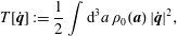 $$\begin{eqnarray}T[\dot{\boldsymbol{q}}]:=\frac{1}{2}\int \text{d}^{3}a\,\unicode[STIX]{x1D70C}_{0}(\boldsymbol{a})\,|\dot{\boldsymbol{q}}|^{2},\end{eqnarray}$$
 where  $\unicode[STIX]{x1D70C}_{0}$ is the mass density attached to the fluid element labelled by $\boldsymbol{a}$ and $\dot{\boldsymbol{q}}$ denotes time differentiation of $\boldsymbol{q}$ at fixed label $\boldsymbol{a}$. Note, in (3.10) $|\dot{\boldsymbol{q}}|^{2}=\dot{q}_{i}\dot{q}^{i}$, where in general $\dot{q}_{i}=g_{ij}\,\dot{q}^{i}$, but we will only consider the cartesian metric where $g_{ij}=\unicode[STIX]{x1D6FF}_{ij}=\unicode[STIX]{x1D702}_{ij}$.
Fluids are assumed to be in local thermodynamic equilibrium and thus can be described by a function  $U(\unicode[STIX]{x1D70C},s)$, an internal energy per unit mass that depends on the specific volume $\unicode[STIX]{x1D70C}^{-1}$ and specific entropy $s$. If a magnetic field $\boldsymbol{B}(\boldsymbol{x},t)$ were present, then we could add dependence on $|\boldsymbol{B}|$ as in Morrison (Reference Morrison1982) to account for pressure anisotropy. (See also Morrison, Lingam & Acevedo (Reference Morrison, Lingam and Acevedo2014), Lingam, Morrison & Wurm (Reference Lingam, Morrison and Wurm2020) where this appears in the context of gyroviscosity.) The internal energy is written in terms of the Eulerian density and entropy (see § 3.3) since we expect the fluid at each Eulerian observation point to be in thermal equilibrium. From $U$ we compute the temperature and pressure according to the usual differentiations, $T=\unicode[STIX]{x2202}U/\unicode[STIX]{x2202}s$ and $p=\unicode[STIX]{x1D70C}^{2}\unicode[STIX]{x2202}U/\unicode[STIX]{x2202}\unicode[STIX]{x1D70C}$. For MHD, the magnetic energy $H_{B}=\int \text{d}^{3}x\,|\boldsymbol{B}|^{2}/2$ in Lagrangian variables would be added. For the ideal fluid, the total internal energy functional is
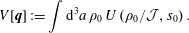 $$\begin{eqnarray}V[\boldsymbol{q}]:=\int \text{d}^{3}a\,\unicode[STIX]{x1D70C}_{0}\,U\left(\unicode[STIX]{x1D70C}_{0}/{\mathcal{J}},s_{0}\right).\end{eqnarray}$$
 Here we have used the fact that a fluid element carries a specific entropy  $s=s_{0}(\boldsymbol{a})$ and a mass determined by $\unicode[STIX]{x1D70C}=\unicode[STIX]{x1D70C}_{0}(\boldsymbol{a})/{\mathcal{J}}$. In § 3.3 we will describe in detail the map from Lagrangian to Eulerian variables.
Thus, the special case of the action principle of (2.72) for the ideal fluid has Lagrange’s Lagrangian  $L[\boldsymbol{q},\dot{\boldsymbol{q}}]=T-V$. Variation of this action gives the Lagrangian equation of motion for the fluid
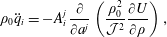 $$\begin{eqnarray}\unicode[STIX]{x1D70C}_{0}\ddot{q}_{i}=-A_{i}^{j}\,\frac{\unicode[STIX]{x2202}}{\unicode[STIX]{x2202}a^{j}}\left(\frac{\unicode[STIX]{x1D70C}_{0}^{2}}{{\mathcal{J}}^{2}}\frac{\unicode[STIX]{x2202}U}{\unicode[STIX]{x2202}\unicode[STIX]{x1D70C}}\right),\end{eqnarray}$$
 with an additional term that describes the  $\boldsymbol{J}\times \boldsymbol{B}$ force in Lagrangian variables for MHD. See, e.g. Newcomb (Reference Newcomb1962) and Morrison (Reference Morrison1998, Reference Morrison2009) for details of this calculation and the MHD extension.
3.2 Hamiltonian formalism in Lagrangian description
Upon defining the momentum density as usual by
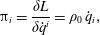 $$\begin{eqnarray}\unicode[STIX]{x03C0}_{i}=\frac{\unicode[STIX]{x1D6FF}L}{\unicode[STIX]{x1D6FF}\dot{q}^{i}}=\unicode[STIX]{x1D70C}_{0}\,\dot{q}_{i},\end{eqnarray}$$
we can obtain the Hamiltonian by Legendre transformation, yielding
 $$\begin{eqnarray}H[\unicode[STIX]{x03C0},\boldsymbol{q}]=T+V=\int \text{d}^{3}a\,\left(\frac{|\unicode[STIX]{x03C0}|^{2}}{2\unicode[STIX]{x1D70C}_{0}}\,+\unicode[STIX]{x1D70C}_{0}U(\unicode[STIX]{x1D70C}_{0}/{\mathcal{J}},s_{0})\right),\end{eqnarray}$$
 where  $|\unicode[STIX]{x03C0}|^{2}=\unicode[STIX]{x03C0}^{i}\unicode[STIX]{x03C0}_{i}=\unicode[STIX]{x03C0}_{i}\unicode[STIX]{x1D702}^{ij}\unicode[STIX]{x03C0}_{j}$. This Hamiltonian with the canonical Poisson bracket,
 $$\begin{eqnarray}\{F,G\}=\int \text{d}^{3}a\,\left(\frac{\unicode[STIX]{x1D6FF}F}{\unicode[STIX]{x1D6FF}q^{i}}\frac{\unicode[STIX]{x1D6FF}G}{\unicode[STIX]{x1D6FF}\unicode[STIX]{x03C0}_{i}}-\frac{\unicode[STIX]{x1D6FF}G}{\unicode[STIX]{x1D6FF}q^{i}}\frac{\unicode[STIX]{x1D6FF}F}{\unicode[STIX]{x1D6FF}\unicode[STIX]{x03C0}_{i}}\right),\end{eqnarray}$$
yields
 $$\begin{eqnarray}\displaystyle & \displaystyle \dot{q}^{i}=\{q^{i},H\}=\unicode[STIX]{x03C0}^{i}\!/\unicode[STIX]{x1D70C}_{0}, & \displaystyle\end{eqnarray}$$
 $$\begin{eqnarray}\displaystyle & \displaystyle \dot{\unicode[STIX]{x03C0}}_{i}=\{\unicode[STIX]{x03C0}_{i},H\}=-A_{i}^{j}\,\frac{\unicode[STIX]{x2202}}{\unicode[STIX]{x2202}a^{j}}\left(\frac{\unicode[STIX]{x1D70C}_{0}^{2}}{{\mathcal{J}}^{2}}\frac{\unicode[STIX]{x2202}U}{\unicode[STIX]{x2202}\unicode[STIX]{x1D70C}}\right). & \displaystyle\end{eqnarray}$$
 Equations (3.16) and (3.17) are equivalent to (3.12). For MHD a term  $H_{B}$ is added to (3.14) (see Newcomb (Reference Newcomb1962), Morrison (Reference Morrison2009)). We will give this explicitly in the constraint context in § 4.2.1 after discussing the Lagrange to Euler map.
3.3 Hamiltonian formalism in Eulerian description via the Lagrange to Euler map
In order to understand how constraints in terms of the Lagrangian variable description relate to those in terms of the Eulerian description, in particular  $\unicode[STIX]{x1D735}\boldsymbol{\cdot }\boldsymbol{v}=0$, it is necessary to understand the mapping from Lagrangian to Eulerian variables. Thus, we record here the relationship between the two unconstrained descriptions, i.e. how the noncanonical Hamiltonian structure of the compressible Euler’s equations relates to the Hamiltonian structure described in § 3.2.
For the ideal fluid, the set of Eulerian variables can be taken to be  $\{\boldsymbol{v},\unicode[STIX]{x1D70C},s\}$, where $\boldsymbol{v}(\boldsymbol{x},t)$ is the velocity field at the Eulerian observation point, $\boldsymbol{x}=(x,y,z)=(x^{1},x^{2},x^{3})$ at time $t$ and, as noted in § 3.1, $\unicode[STIX]{x1D70C}(\boldsymbol{x},t)$ is the mass density and $s(\boldsymbol{x},t)$ is the specific entropy. In order to describe magnetofluids the magnetic field $\boldsymbol{B}(\boldsymbol{x},t)$ would be appended to this set. It is most important to distinguish between the Lagrangian fluid element position and label variables, $\boldsymbol{q}$ and $\boldsymbol{a}$, and the Eulerian observation point $\boldsymbol{x}$, the latter two being independent variables. Confusion exists in the literature because some authors use the same symbol for the Lagrangian coordinate $\boldsymbol{q}$ and the Eulerian observation point $\boldsymbol{x}$.
The Lagrangian and Eulerian descriptions must clearly be related and, indeed, knowing  $\boldsymbol{q}(\boldsymbol{a},t)$ we can obtain $\boldsymbol{v}(\boldsymbol{x},t)$. If one were to insert a velocity probe into a fluid at $(\boldsymbol{x},t)$ then one would measure the velocity of the fluid element that happened to be at that position at that time. Thus it is clear that $\dot{\boldsymbol{q}}(\boldsymbol{a},t)=\boldsymbol{v}(\boldsymbol{x},t)$, where recall the overdot means the time derivative at constant $\boldsymbol{a}$. But, which fluid element will be at $\boldsymbol{x}$ at time $t$? Evidently $\boldsymbol{x}=\boldsymbol{q}(\boldsymbol{a},t)$, which upon inversion yields the label of that element that will be measured, $\boldsymbol{a}=\boldsymbol{q}^{-1}(\boldsymbol{x},t)$. Thus, the Eulerian velocity field is given by
 $$\begin{eqnarray}\boldsymbol{v}(\boldsymbol{x},t)=\left.\dot{\boldsymbol{q}}(\boldsymbol{a},t)\right|_{\boldsymbol{a}=\boldsymbol{q}^{-1}(\boldsymbol{x},t)}=\dot{\boldsymbol{q}}\circ \boldsymbol{q}^{-1}(\boldsymbol{x},t).\end{eqnarray}$$
 Properties can be attached to fluid elements, just as a given mass is identified with a given particle in mechanics. For a continuum system it is natural to attach a mass density,  $\unicode[STIX]{x1D70C}_{0}(\boldsymbol{a})$, to the element labelled by $\boldsymbol{a}$. Whence the element of mass in a given volume is given by $\unicode[STIX]{x1D70C}_{0}\text{d}^{3}a$ and this amount of mass is preserved by the flow, i.e. $\unicode[STIX]{x1D70C}(\boldsymbol{x},t)\text{d}^{3}x=\unicode[STIX]{x1D70C}_{0}(\boldsymbol{a})\text{d}^{3}a$. Because the locus of points of material surfaces move with the fluid are determined by $\boldsymbol{q}$, an initial volume element $\text{d}^{3}a$ maps into a volume element $\text{d}^{3}x$ at time $t$ according to
 $$\begin{eqnarray}\text{d}^{3}x={\mathcal{J}}\text{d}^{3}a.\end{eqnarray}$$
 Thus, using (3.19) we obtain  $\unicode[STIX]{x1D70C}_{0}=\unicode[STIX]{x1D70C}{\mathcal{J}}$ as used in § 3.1.
Other quantities could be attached to a fluid element; for the ideal fluid, entropy per unit mass,  $s(\boldsymbol{x},t)$, is such a quantity. The assumption that each fluid element is isentropic then amounts to $s=s_{0}$. Similarly, for MHD a magnetic field, $B_{0}(\boldsymbol{a})$, can be attached, and then the frozen flux assumption yields $B\boldsymbol{\cdot }\text{d}^{2}x=B_{0}\boldsymbol{\cdot }\text{d}^{2}a$. An initial area element $\text{d}^{2}a$ maps into an area element $\text{d}^{2}x$ at time $t$ according to
 $$\begin{eqnarray}(\text{d}^{2}x)_{i}=A_{i}^{j}\,(\text{d}^{2}a)_{j}.\end{eqnarray}$$
 Using (3.20) we obtain  ${\mathcal{J}}B^{i}=B_{0}^{j}\,\unicode[STIX]{x2202}q^{i}/\unicode[STIX]{x2202}a^{j}$.
Sometimes it is convenient to use another set of Eulerian density variables:  $\{\boldsymbol{M},\unicode[STIX]{x1D70C},\unicode[STIX]{x1D70E},\boldsymbol{B}\}$, where $\unicode[STIX]{x1D70E}=\unicode[STIX]{x1D70C}s$ is the entropy per unit volume, and $\boldsymbol{M}=\unicode[STIX]{x1D70C}\boldsymbol{v}$ is the momentum density. These Eulerian variables can be represented by using the Dirac delta function to ‘pluck out’ the fluid element that happens to be at the Eulerian observation point $\boldsymbol{x}$ at time $t$. For example, the mass density $\unicode[STIX]{x1D70C}(\boldsymbol{x},t)$ is obtained by
 $$\begin{eqnarray}\unicode[STIX]{x1D70C}(\boldsymbol{x},t)=\int \text{d}^{3}a\,\unicode[STIX]{x1D70C}_{0}(\boldsymbol{a})\,\unicode[STIX]{x1D6FF}(\boldsymbol{x}-\boldsymbol{q}(\boldsymbol{a},t))=\left.\frac{\unicode[STIX]{x1D70C}_{0}}{{\mathcal{J}}}\right|_{\boldsymbol{a}=\boldsymbol{q}^{-1}(\boldsymbol{x},t)}\!.\end{eqnarray}$$
 The density one observes at  $\boldsymbol{x}$ at time $t$ will be the one attached to the fluid element that happens to be there then, and this fluid element has a label given by solving $\boldsymbol{x}=\boldsymbol{q}(\boldsymbol{a},t)$. The second equality of (3.21) is obtained by using the three-dimensional version of the delta function identity $\unicode[STIX]{x1D6FF}(f(x))=\sum _{i}\unicode[STIX]{x1D6FF}(x-x_{i})/|\,f^{\prime }(x_{i})|$, where $f(x_{i})=0$. Similarly, the entropy per unit volume is given by
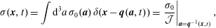 $$\begin{eqnarray}\unicode[STIX]{x1D70E}(\boldsymbol{x},t)=\int \text{d}^{3}a\,\unicode[STIX]{x1D70E}_{0}(\boldsymbol{a})\,\unicode[STIX]{x1D6FF}(\boldsymbol{x}-\boldsymbol{q}(\boldsymbol{a},t))=\left.\frac{\unicode[STIX]{x1D70E}_{0}}{{\mathcal{J}}}\right|_{\boldsymbol{a}=\boldsymbol{q}^{-1}(\boldsymbol{x},t)},\end{eqnarray}$$
 which is consistent with  $\unicode[STIX]{x1D70E}_{0}(\boldsymbol{a})=\unicode[STIX]{x1D70C}_{0}(\boldsymbol{a})s_{0}(\boldsymbol{a})$ and $s(\boldsymbol{x},t)=s_{0}(\boldsymbol{a})|_{\boldsymbol{a}=\boldsymbol{q}^{-1}(\boldsymbol{x},t)}$, where the latter means $s$ is constant along a Lagrangian orbit. Proceeding, the momentum density, $\boldsymbol{M}=(M_{1},M_{2},M_{3})$, is related to the Lagrangian canonical momentum (defined in § 3.2) by
 $$\begin{eqnarray}\boldsymbol{M}(\boldsymbol{x},t)=\int \!\text{d}^{3}a\,\unicode[STIX]{x03C0}(\boldsymbol{a},t)\,\unicode[STIX]{x1D6FF}(\boldsymbol{x}-\boldsymbol{q}(\boldsymbol{a},t))=\left.\frac{\unicode[STIX]{x03C0}(\boldsymbol{a},t)}{{\mathcal{J}}}\right|_{\boldsymbol{a}=\boldsymbol{q}^{-1}(\boldsymbol{x},t)},\end{eqnarray}$$
 where for the ideal fluid and MHD,  $\unicode[STIX]{x03C0}(\boldsymbol{a},t)=(\unicode[STIX]{x03C0}_{1},\unicode[STIX]{x03C0}_{2},\unicode[STIX]{x03C0}_{3})=\unicode[STIX]{x1D70C}_{0}\dot{\boldsymbol{q}}$. Lastly,
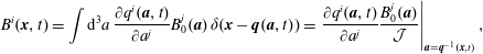 $$\begin{eqnarray}B^{i}(\boldsymbol{x},t)=\int \text{d}^{3}a\,\frac{\unicode[STIX]{x2202}q^{i}(\boldsymbol{a},t)}{\unicode[STIX]{x2202}a^{j}}B_{0}^{j}(\boldsymbol{a})\,\unicode[STIX]{x1D6FF}(\boldsymbol{x}-\boldsymbol{q}(\boldsymbol{a},t))=\left.\frac{\unicode[STIX]{x2202}q^{i}(\boldsymbol{a},t)}{\unicode[STIX]{x2202}a^{j}}\frac{B_{0}^{j}(\boldsymbol{a})}{{\mathcal{J}}}\right|_{\boldsymbol{a}=\boldsymbol{q}^{-1}(\boldsymbol{x},t)},\end{eqnarray}$$
for the components of the magnetic field. It may be unfamiliar to view the magnetic field as density, but in MHD it obeys a conservation law. Geometrically, however, it naturally satisfies the equations of a vector density associated with a differential 2-form as was observed in Morrison (Reference Morrison1982) and Tur & Yanovsky (Reference Tur and Yanovsky1993).
To obtain the noncanonical Eulerian Poisson bracket we consider functionals  $F[\boldsymbol{q},\unicode[STIX]{x03C0}]$ that are restricted so as to obtain their dependence on $\boldsymbol{q}$ and $\unicode[STIX]{x03C0}$ only through the Eulerian variables. Upon setting $F[\boldsymbol{q},\unicode[STIX]{x03C0}]=\bar{F}[\boldsymbol{v},\unicode[STIX]{x1D70C},\unicode[STIX]{x1D70E}]$, equating variations of both sides,
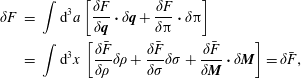 $$\begin{eqnarray}\displaystyle \unicode[STIX]{x1D6FF}F & = & \displaystyle \int \text{d}^{3}a\left[\frac{\unicode[STIX]{x1D6FF}F}{\unicode[STIX]{x1D6FF}\boldsymbol{q}}\boldsymbol{\cdot }\unicode[STIX]{x1D6FF}\boldsymbol{q}+\frac{\unicode[STIX]{x1D6FF}F}{\unicode[STIX]{x1D6FF}\unicode[STIX]{x03C0}}\boldsymbol{\cdot }\unicode[STIX]{x1D6FF}\unicode[STIX]{x03C0}\right]\nonumber\\ \displaystyle & = & \displaystyle \int \text{d}^{3}x\,\left[\frac{\unicode[STIX]{x1D6FF}\bar{F}}{\unicode[STIX]{x1D6FF}\unicode[STIX]{x1D70C}}\unicode[STIX]{x1D6FF}\unicode[STIX]{x1D70C}+\frac{\unicode[STIX]{x1D6FF}\bar{F}}{\unicode[STIX]{x1D6FF}\unicode[STIX]{x1D70E}}\unicode[STIX]{x1D6FF}\unicode[STIX]{x1D70E}+\frac{\unicode[STIX]{x1D6FF}\bar{F}}{\unicode[STIX]{x1D6FF}\boldsymbol{M}}\boldsymbol{\cdot }\unicode[STIX]{x1D6FF}\boldsymbol{M}\right]=\unicode[STIX]{x1D6FF}\bar{F},\end{eqnarray}$$
 varying the expressions (3.21), (3.22) and (3.23), substituting the result into (3.25) and equating the independent coefficients of  $\unicode[STIX]{x1D6FF}\boldsymbol{q}$ and $\unicode[STIX]{x1D6FF}\unicode[STIX]{x03C0}$, we obtain
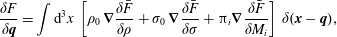 $$\begin{eqnarray}\displaystyle & \displaystyle \frac{\unicode[STIX]{x1D6FF}F}{\unicode[STIX]{x1D6FF}\boldsymbol{q}}=\int \text{d}^{3}x\,\left[\unicode[STIX]{x1D70C}_{0}\,\unicode[STIX]{x1D735}\frac{\unicode[STIX]{x1D6FF}\bar{F}}{\unicode[STIX]{x1D6FF}\unicode[STIX]{x1D70C}}+\unicode[STIX]{x1D70E}_{0}\,\unicode[STIX]{x1D735}\frac{\unicode[STIX]{x1D6FF}\bar{F}}{\unicode[STIX]{x1D6FF}\unicode[STIX]{x1D70E}}+\unicode[STIX]{x03C0}_{i}\unicode[STIX]{x1D735}\frac{\unicode[STIX]{x1D6FF}\bar{F}}{\unicode[STIX]{x1D6FF}M_{i}}\right]\,\unicode[STIX]{x1D6FF}(\boldsymbol{x}-\boldsymbol{q}), & \displaystyle\end{eqnarray}$$
 $$\begin{eqnarray}\displaystyle & \displaystyle \frac{\unicode[STIX]{x1D6FF}F}{\unicode[STIX]{x1D6FF}\unicode[STIX]{x03C0}}=\int \text{d}^{3}x\,\frac{\unicode[STIX]{x1D6FF}\bar{F}}{\unicode[STIX]{x1D6FF}\boldsymbol{M}}\,\unicode[STIX]{x1D6FF}(\boldsymbol{x}-\boldsymbol{q}). & \displaystyle\end{eqnarray}$$
 (See Morrison (Reference Morrison1998) and Morrison & Greene (Reference Morrison and Greene1980) for details.) Upon substitution of (3.26) and (3.27), expressions of the functional chain rule that relate Lagrangian functional derivatives to the Eulerian functional derivates, into (3.15) yields the following bracket expressed entirely in terms of the Eulerian fields  $\{\boldsymbol{M},\unicode[STIX]{x1D70C},\unicode[STIX]{x1D70E}\}$:
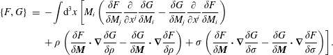 $$\begin{eqnarray}\displaystyle \hspace{-36.0pt}\{F,G\} & = & \displaystyle -\int \text{d}^{3}x\,\Bigg[M_{i}\left(\frac{\unicode[STIX]{x1D6FF}F}{\unicode[STIX]{x1D6FF}M_{j}}\frac{\unicode[STIX]{x2202}}{\unicode[STIX]{x2202}x^{j}}\frac{\unicode[STIX]{x1D6FF}G}{\unicode[STIX]{x1D6FF}M_{i}}-\frac{\unicode[STIX]{x1D6FF}G}{\unicode[STIX]{x1D6FF}M_{j}}\frac{\unicode[STIX]{x2202}}{\unicode[STIX]{x2202}x^{j}}\frac{\unicode[STIX]{x1D6FF}F}{\unicode[STIX]{x1D6FF}M_{i}}\right)\nonumber\\ \displaystyle \hspace{-36.0pt} & & \displaystyle +\,\unicode[STIX]{x1D70C}\,\Bigg(\frac{\unicode[STIX]{x1D6FF}F}{\unicode[STIX]{x1D6FF}\boldsymbol{M}}\boldsymbol{\cdot }\unicode[STIX]{x1D735}\frac{\unicode[STIX]{x1D6FF}G}{\unicode[STIX]{x1D6FF}\unicode[STIX]{x1D70C}}-\frac{\unicode[STIX]{x1D6FF}G}{\unicode[STIX]{x1D6FF}\boldsymbol{M}}\boldsymbol{\cdot }\unicode[STIX]{x1D735}\frac{\unicode[STIX]{x1D6FF}F}{\unicode[STIX]{x1D6FF}\unicode[STIX]{x1D70C}}\Bigg)+\unicode[STIX]{x1D70E}\,\Bigg(\frac{\unicode[STIX]{x1D6FF}F}{\unicode[STIX]{x1D6FF}\boldsymbol{M}}\boldsymbol{\cdot }\unicode[STIX]{x1D735}\frac{\unicode[STIX]{x1D6FF}G}{\unicode[STIX]{x1D6FF}\unicode[STIX]{x1D70E}}-\frac{\unicode[STIX]{x1D6FF}G}{\unicode[STIX]{x1D6FF}\boldsymbol{M}}\boldsymbol{\cdot }\unicode[STIX]{x1D735}\frac{\unicode[STIX]{x1D6FF}F}{\unicode[STIX]{x1D6FF}\unicode[STIX]{x1D70E}}\Bigg)\Bigg].\end{eqnarray}$$
 In (3.28) we have dropped the overbars on the Eulerian functional derivatives. The bracket for MHD is the above with the addition of the following term, which is obtained by adding a  $\boldsymbol{B}$ contribution to (3.25):
 $$\begin{eqnarray}\displaystyle \{F,G\}_{B} & = & \displaystyle -\int \text{d}^{3}x\,\left[\boldsymbol{B}\boldsymbol{\cdot }\left(\frac{\unicode[STIX]{x1D6FF}F}{\unicode[STIX]{x1D6FF}\boldsymbol{M}}\boldsymbol{\cdot }\unicode[STIX]{x1D735}\frac{\unicode[STIX]{x1D6FF}G}{\unicode[STIX]{x1D6FF}\boldsymbol{B}}-\frac{\unicode[STIX]{x1D6FF}G}{\unicode[STIX]{x1D6FF}\boldsymbol{M}}\boldsymbol{\cdot }\unicode[STIX]{x1D735}\frac{\unicode[STIX]{x1D6FF}F}{\unicode[STIX]{x1D6FF}\boldsymbol{B}}\right)\right.\nonumber\\ \displaystyle & & \displaystyle \left.+\,\boldsymbol{B}\boldsymbol{\cdot }\left(\unicode[STIX]{x1D735}\left(\frac{\unicode[STIX]{x1D6FF}F}{\unicode[STIX]{x1D6FF}\boldsymbol{M}}\right)\boldsymbol{\cdot }\frac{\unicode[STIX]{x1D6FF}G}{\unicode[STIX]{x1D6FF}\boldsymbol{B}}-\unicode[STIX]{x1D735}\left(\frac{\unicode[STIX]{x1D6FF}G}{\unicode[STIX]{x1D6FF}\boldsymbol{M}}\right)\boldsymbol{\cdot }\frac{\unicode[STIX]{x1D6FF}F}{\unicode[STIX]{x1D6FF}\boldsymbol{B}}\right)\right],\end{eqnarray}$$
 where dyadic notation is used; for example,  $\boldsymbol{B}\boldsymbol{\cdot }[\unicode[STIX]{x1D735}(\boldsymbol{D})\boldsymbol{\cdot }\boldsymbol{C}]=\sum _{i,j}B_{i}C_{j}\unicode[STIX]{x2202}D_{j}/\unicode[STIX]{x2202}x_{i}$, for vectors $\boldsymbol{B},\boldsymbol{D}$, and $\boldsymbol{C}$. Alternatively, the bracket in terms of $\{\boldsymbol{v},\unicode[STIX]{x1D70C},s,\boldsymbol{B}\}$ is obtained using chain rule expressions, e.g.
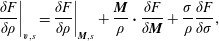 $$\begin{eqnarray}\frac{\unicode[STIX]{x1D6FF}F}{\unicode[STIX]{x1D6FF}\unicode[STIX]{x1D70C}}\Bigg|_{\boldsymbol{v},s}=\frac{\unicode[STIX]{x1D6FF}F}{\unicode[STIX]{x1D6FF}\unicode[STIX]{x1D70C}}\Bigg|_{\boldsymbol{M},s}+\frac{\boldsymbol{M}}{\unicode[STIX]{x1D70C}}\boldsymbol{\cdot }\frac{\unicode[STIX]{x1D6FF}F}{\unicode[STIX]{x1D6FF}\boldsymbol{M}}+\frac{\unicode[STIX]{x1D70E}}{\unicode[STIX]{x1D70C}}\frac{\unicode[STIX]{x1D6FF}F}{\unicode[STIX]{x1D6FF}\unicode[STIX]{x1D70E}},\end{eqnarray}$$
yielding
 $$\begin{eqnarray}\displaystyle \{F,G\} & = & \displaystyle -\int \text{d}^{3}x\,\Bigg[\Bigg(\frac{\unicode[STIX]{x1D6FF}F}{\unicode[STIX]{x1D6FF}\unicode[STIX]{x1D70C}}\unicode[STIX]{x1D735}\boldsymbol{\cdot }\frac{\unicode[STIX]{x1D6FF}G}{\unicode[STIX]{x1D6FF}\boldsymbol{v}}-\frac{\unicode[STIX]{x1D6FF}G}{\unicode[STIX]{x1D6FF}\unicode[STIX]{x1D70C}}\unicode[STIX]{x1D735}\boldsymbol{\cdot }\frac{\unicode[STIX]{x1D6FF}F}{\unicode[STIX]{x1D6FF}\boldsymbol{v}}\Bigg)+\Bigg(\frac{\unicode[STIX]{x1D735}\times \boldsymbol{v}}{\unicode[STIX]{x1D70C}}\boldsymbol{\cdot }\frac{\unicode[STIX]{x1D6FF}G}{\unicode[STIX]{x1D6FF}\boldsymbol{v}}\times \frac{\unicode[STIX]{x1D6FF}F}{\unicode[STIX]{x1D6FF}\boldsymbol{v}}\Bigg)\nonumber\\ \displaystyle & & \displaystyle +\,\frac{\unicode[STIX]{x1D735}s}{\unicode[STIX]{x1D70C}}\boldsymbol{\cdot }\Bigg(\frac{\unicode[STIX]{x1D6FF}F}{\unicode[STIX]{x1D6FF}s}\frac{\unicode[STIX]{x1D6FF}G}{\unicode[STIX]{x1D6FF}\boldsymbol{v}}-\frac{\unicode[STIX]{x1D6FF}G}{\unicode[STIX]{x1D6FF}s}\frac{\unicode[STIX]{x1D6FF}F}{\unicode[STIX]{x1D6FF}\boldsymbol{v}}\Bigg)\Bigg],\end{eqnarray}$$
and
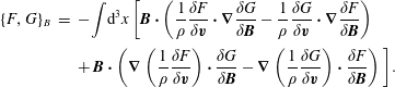 $$\begin{eqnarray}\displaystyle \{F,G\}_{B} & = & \displaystyle -\int \text{d}^{3}x\,\Bigg[\boldsymbol{B}\boldsymbol{\cdot }\left(\frac{1}{\unicode[STIX]{x1D70C}}\frac{\unicode[STIX]{x1D6FF}F}{\unicode[STIX]{x1D6FF}\boldsymbol{v}}\boldsymbol{\cdot }\unicode[STIX]{x1D735}\frac{\unicode[STIX]{x1D6FF}G}{\unicode[STIX]{x1D6FF}\boldsymbol{B}}-\frac{1}{\unicode[STIX]{x1D70C}}\frac{\unicode[STIX]{x1D6FF}G}{\unicode[STIX]{x1D6FF}\boldsymbol{v}}\boldsymbol{\cdot }\unicode[STIX]{x1D735}\frac{\unicode[STIX]{x1D6FF}F}{\unicode[STIX]{x1D6FF}\boldsymbol{B}}\right)\nonumber\\ \displaystyle & & \displaystyle +\,\boldsymbol{B}\boldsymbol{\cdot }\left(\unicode[STIX]{x1D735}\left(\frac{1}{\unicode[STIX]{x1D70C}}\frac{\unicode[STIX]{x1D6FF}F}{\unicode[STIX]{x1D6FF}\boldsymbol{v}}\right)\boldsymbol{\cdot }\frac{\unicode[STIX]{x1D6FF}G}{\unicode[STIX]{x1D6FF}\boldsymbol{B}}-\unicode[STIX]{x1D735}\left(\frac{1}{\unicode[STIX]{x1D70C}}\frac{\unicode[STIX]{x1D6FF}G}{\unicode[STIX]{x1D6FF}\boldsymbol{v}}\right)\boldsymbol{\cdot }\frac{\unicode[STIX]{x1D6FF}F}{\unicode[STIX]{x1D6FF}\boldsymbol{B}}\right)\Bigg].\end{eqnarray}$$
The bracket of (3.31) plus that of (3.32) with the Hamiltonian
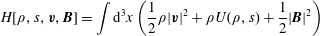 $$\begin{eqnarray}H[\unicode[STIX]{x1D70C},s,\boldsymbol{v},\boldsymbol{B}]=\int \text{d}^{3}x\left(\frac{1}{2}\unicode[STIX]{x1D70C}|\boldsymbol{v}|^{2}+\unicode[STIX]{x1D70C}U(\unicode[STIX]{x1D70C},s)+\frac{1}{2}|\boldsymbol{B}|^{2}\right)\end{eqnarray}$$
 gives the Eulerian version of MHD in Hamiltonian form,  $\unicode[STIX]{x2202}\boldsymbol{v}/\unicode[STIX]{x2202}t=\{\boldsymbol{v},H\}$, etc., and similarly using (3.28) plus (3.29) with the Hamiltonian expressed in terms of $(\boldsymbol{M},\unicode[STIX]{x1D70C},\unicode[STIX]{x1D70E},\boldsymbol{B})$. Ideal fluid follows upon neglecting the $\boldsymbol{B}$ terms.
3.4 Constants of motion: Eulerian versus Lagrangian
In order to compare the imposition of constraints in the Lagrangian and Eulerian descriptions, it is necessary to compare Lagrangian and Eulerian conservations laws. This is because constraints, when enforced, are conserved quantities. The comparison is not trivial because time-independent quantities in the Eulerian description can be time dependent in the Lagrangian description.
Consider a Lagrangian function  $f(\boldsymbol{a},t)$, typical of the Lagrangian variable description, and the relation $\boldsymbol{x}=\boldsymbol{q}(\boldsymbol{a},t)$, which relates an Eulerian observation point $\boldsymbol{x}$ to a corresponding fluid element trajectory value. The function $f$ can be written in either picture by composition, as follows:
 $$\begin{eqnarray}f(\boldsymbol{a},t)=\tilde{f}(\boldsymbol{x},t)=\tilde{f}(\boldsymbol{q}(\boldsymbol{a},t),t),\end{eqnarray}$$
where we will use a tilde to indicated the Eulerian form of a Lagrangian function. Application of the chain rule gives
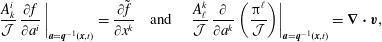 $$\begin{eqnarray}\left.\frac{A_{k}^{i}}{{\mathcal{J}}}\,\frac{\unicode[STIX]{x2202}f}{\unicode[STIX]{x2202}a^{i}}\,\right|_{\boldsymbol{a}=\boldsymbol{q}^{-1}(\boldsymbol{x},t)}=\frac{\unicode[STIX]{x2202}\tilde{f}}{\unicode[STIX]{x2202}x^{k}}\quad \text{and}\quad \left.\frac{A_{\ell }^{k}}{{\mathcal{J}}}\,\frac{\unicode[STIX]{x2202}}{\unicode[STIX]{x2202}a^{k}}\left(\frac{\unicode[STIX]{x03C0}^{\ell }}{{\mathcal{J}}}\right)\right|_{\boldsymbol{a}=\boldsymbol{q}^{-1}(\boldsymbol{x},t)}=\unicode[STIX]{x1D735}\boldsymbol{\cdot }\boldsymbol{v},\end{eqnarray}$$
with the second equality of (3.35) being a special case of the first. Similarly,
 $$\begin{eqnarray}\left.{\dot{f}}\,\right|_{\boldsymbol{a}=\boldsymbol{q}^{-1}(\boldsymbol{x},t)}=\frac{\unicode[STIX]{x2202}\tilde{f}}{\unicode[STIX]{x2202}t}+\left.\dot{q}^{i}(\boldsymbol{a},t)\,\frac{\unicode[STIX]{x2202}\tilde{f}}{\unicode[STIX]{x2202}x^{i}}\,\right|_{\boldsymbol{a}=\boldsymbol{q}^{-1}(\boldsymbol{x},t)}=\frac{\unicode[STIX]{x2202}\tilde{f}}{\unicode[STIX]{x2202}t}+\boldsymbol{v}\boldsymbol{\cdot }\unicode[STIX]{x1D735}\tilde{f}(\boldsymbol{x},t),\end{eqnarray}$$
 where recall an overdot denotes the time derivative at constant  $\boldsymbol{a}$, $\unicode[STIX]{x2202}/\unicode[STIX]{x2202}t$ denotes the time derivative at constant $\boldsymbol{x}$ and $\unicode[STIX]{x1D735}$ is the Eulerian gradient with components $\unicode[STIX]{x2202}/\unicode[STIX]{x2202}x^{i}$ as used in (3.35). Because the Jacobian determinant ${\mathcal{J}}$ is composed of derivatives of $\boldsymbol{q}$, we have ${\mathcal{J}}(\boldsymbol{a},t)|_{\boldsymbol{a}=\boldsymbol{q}^{-1}(\boldsymbol{x},t)}=\tilde{{\mathcal{J}}}(\boldsymbol{x},t)$, whence one obtains a formula due to Euler (see e.g. Serrin Reference Serrin and Flügge1959),
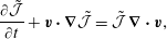 $$\begin{eqnarray}\frac{\unicode[STIX]{x2202}\tilde{{\mathcal{J}}}}{\unicode[STIX]{x2202}t}+\boldsymbol{v}\boldsymbol{\cdot }\unicode[STIX]{x1D735}\tilde{{\mathcal{J}}}=\tilde{{\mathcal{J}}}\,\unicode[STIX]{x1D735}\boldsymbol{\cdot }\boldsymbol{v},\end{eqnarray}$$
which can be compared to its Lagrangian version of (3.7).
Now, consider a conservation law in the Lagrangian variable description,
 $$\begin{eqnarray}\dot{{\mathcal{D}}}_{L}+\frac{\unicode[STIX]{x2202}\unicode[STIX]{x1D6E4}_{{\mathcal{D}}_{L}}^{i}}{\unicode[STIX]{x2202}a^{i}}=0,\end{eqnarray}$$
 where the density  ${\mathcal{D}}_{L}(\boldsymbol{a},t)$ has the associated flux $\unicode[STIX]{x1D6E4}_{{\mathcal{D}}_{L}}$. Then, the associated conserved quantity is
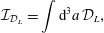 $$\begin{eqnarray}{\mathcal{I}}_{{\mathcal{D}}_{L}}=\int \text{d}^{3}a\,{\mathcal{D}}_{L},\end{eqnarray}$$
 which satisfies  $\text{d}{\mathcal{I}}_{{\mathcal{D}}_{L}}/\text{d}t=0$ provided surface terms vanish. Similarly, an Eulerian conservation law with density ${\mathcal{D}}_{E}$ and flux $\unicode[STIX]{x1D6E4}_{{\mathcal{D}}_{E}}$ is
 $$\begin{eqnarray}\frac{\unicode[STIX]{x2202}{\mathcal{D}}_{E}}{\unicode[STIX]{x2202}t}+\frac{\unicode[STIX]{x2202}\unicode[STIX]{x1D6E4}_{{\mathcal{D}}_{E}}^{i}}{\unicode[STIX]{x2202}x^{i}}=0\end{eqnarray}$$
and the following is similarly constant in time:
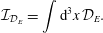 $$\begin{eqnarray}{\mathcal{I}}_{{\mathcal{D}}_{E}}=\int \text{d}^{3}x\,{\mathcal{D}}_{E}.\end{eqnarray}$$
The relationship between the two conservation laws (3.38) and (3.40) can be obtained by defining
 $$\begin{eqnarray}\tilde{{\mathcal{D}}}_{L}={\mathcal{J}}{\mathcal{D}}_{E},\quad \tilde{\unicode[STIX]{x1D6E4}}_{{\mathcal{D}}_{L}}^{i}=A_{k}^{i}\,\bar{\unicode[STIX]{x1D6E4}}_{{\mathcal{D}}_{E}}^{k},\quad \text{and}\quad \unicode[STIX]{x1D6E4}_{{\mathcal{D}}_{E}}=\bar{\unicode[STIX]{x1D6E4}}_{{\mathcal{D}}_{E}}+\boldsymbol{v}\,{\mathcal{D}}_{E},\end{eqnarray}$$
 and their equivalence follows from (3.7), (3.36), and (3.37). Given a Lagrangian conservation law, one can use (3.42) to obtain a corresponding Eulerian conservation law. The density  ${\mathcal{D}}_{E}$ is obtained from the first equation of (3.42), a piece of the Eulerian flux $\bar{\unicode[STIX]{x1D6E4}}_{{\mathcal{D}}_{E}}$ from the second, which then can be substituted into the third equation of (3.42) to obtain the complete Eulerian flux $\unicode[STIX]{x1D6E4}_{{\mathcal{D}}_{E}}$. An Eulerian conservation law is most useful when one can write ${\mathcal{D}}_{E}$ and $\unicode[STIX]{x1D6E4}_{{\mathcal{D}}_{E}}$ entirely in terms of the Eulerian variables of the fluid.
The simplest case occurs when  ${\mathcal{D}}_{L}$ only depends on $\boldsymbol{a}$, in which case the corresponding flux is zero and $\unicode[STIX]{x2202}{\mathcal{D}}_{L}/\unicode[STIX]{x2202}t=0$ and $\text{d}{\mathcal{I}}_{{\mathcal{D}}_{L}}/\text{d}t=0$ follow directly because (3.39) has no time dependence whatsoever. Any attribute attached to a fluid element only depends on the label $\boldsymbol{a}$ and this has a trivial conservation law of this form. However, such trivial Lagrangian conservation laws yield non-trivial Eulerian conservation laws. Observe, even though $\bar{\unicode[STIX]{x1D6E4}}_{{\mathcal{D}}_{E}}\equiv 0$ by (3.42), $\unicode[STIX]{x1D6E4}_{{\mathcal{D}}_{E}}=\boldsymbol{v}{\mathcal{D}}_{E}\neq 0$. Consider the case of the entropy where ${\mathcal{D}}_{L}=s_{0}(\boldsymbol{a})$, whence $s(\boldsymbol{x},t)=s_{0}(\boldsymbol{a}(\boldsymbol{x},t))$ and by (3.36),
 $$\begin{eqnarray}\frac{\unicode[STIX]{x2202}s}{\unicode[STIX]{x2202}t}+\boldsymbol{v}\boldsymbol{\cdot }\unicode[STIX]{x1D735}s=0,\end{eqnarray}$$
 with the quantity  $s=s_{0}/{\mathcal{J}}$ being according to (3.42) the Eulerian conserved density, as can be verified using (3.37). But, as it stands, this density cannot be written in terms of Eulerian fluid variables. However, $\unicode[STIX]{x1D70E}_{0}=\unicode[STIX]{x1D70C}_{0}s_{0}$ is also a trivial Lagrangian conserved density and according to (3.42) we have the Eulerian density $\unicode[STIX]{x1D70C}_{0}s_{0}/{\mathcal{J}}=\unicode[STIX]{x1D70C}s=\unicode[STIX]{x1D70E}$ that satisfies
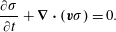 $$\begin{eqnarray}\frac{\unicode[STIX]{x2202}\unicode[STIX]{x1D70E}}{\unicode[STIX]{x2202}t}+\unicode[STIX]{x1D735}\boldsymbol{\cdot }(\boldsymbol{v}\unicode[STIX]{x1D70E})=0.\end{eqnarray}$$
 Thus, it follows that any advected scalar has an associated conserved quantity obtained by multiplication by  $\unicode[STIX]{x1D70C}$.
As another example, consider the quantity  $B_{0}^{i}\unicode[STIX]{x2202}q^{j}/\unicode[STIX]{x2202}a^{i}$. This quantity is the limit displacement between two nearby fluid elements, i.e. $\boldsymbol{q}(\boldsymbol{a},t)-\boldsymbol{q}(\boldsymbol{a}+\unicode[STIX]{x1D6FF}\boldsymbol{a},t)$ along the initial magnetic field as $\unicode[STIX]{x1D6FF}\boldsymbol{a}\rightarrow 0$. Evidently,
 $$\begin{eqnarray}\dot{\left(B_{0}^{i}\frac{\unicode[STIX]{x2202}q^{j}}{\unicode[STIX]{x2202}a^{i}}\right)}=B_{0}^{i}\frac{\unicode[STIX]{x2202}\dot{q}^{j}}{\unicode[STIX]{x2202}a^{i}}=\frac{\unicode[STIX]{x2202}}{\unicode[STIX]{x2202}a^{i}}(B_{0}^{i}\dot{q}^{j}),\end{eqnarray}$$
 where the second equality follows if the initial magnetic field is divergence free. This is of course another trivial conservation law, for the time derivative of a density that is a divergence will always be a divergence. However, let us see what this becomes in the Eulerian description. According to (3.42) the corresponding Eulerian density is  ${\mathcal{D}}_{E}={\mathcal{D}}_{L}/{\mathcal{J}}$; so, the density associated with this trivial conservation law (3.45) is
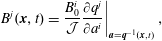 $$\begin{eqnarray}B^{j}(\boldsymbol{x},t)=\left.\frac{B_{0}^{i}}{{\mathcal{J}}}\frac{\unicode[STIX]{x2202}q^{j}}{\unicode[STIX]{x2202}a^{i}}\right|_{\boldsymbol{a}=\boldsymbol{q}^{-1}(\boldsymbol{x},t)},\end{eqnarray}$$
which as we saw in § 3.3 is the expression one gets for the MHD magnetic field because of flux conservation. That the divergence-free magnetic field satisfies a conservation law is clear from
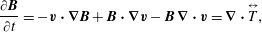 $$\begin{eqnarray}\frac{\unicode[STIX]{x2202}\boldsymbol{B}}{\unicode[STIX]{x2202}t}=-\boldsymbol{v}\boldsymbol{\cdot }\unicode[STIX]{x1D735}\boldsymbol{B}+\boldsymbol{B}\boldsymbol{\cdot }\unicode[STIX]{x1D735}\boldsymbol{v}-\boldsymbol{B}\,\unicode[STIX]{x1D735}\boldsymbol{\cdot }\boldsymbol{v}=\unicode[STIX]{x1D735}\boldsymbol{\cdot }\overset{\leftrightarrow }{T},\end{eqnarray}$$
 where the tensor  $\overset{\leftrightarrow }{T}$ of the last equality is
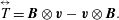 $$\begin{eqnarray}\overset{\leftrightarrow }{T}=\boldsymbol{B}\otimes \boldsymbol{v}-\boldsymbol{v}\otimes \boldsymbol{B}.\end{eqnarray}$$
Thus we have another instance where a trivial Lagrangian conservation law leads to a non-trivial Eulerian one.
Although  $B_{0}^{i}\unicode[STIX]{x2202}q^{j}/\unicode[STIX]{x2202}a^{i}$ does not map into an expression entirely in terms of our set of Eulerian variables, we can divide it by $\unicode[STIX]{x1D70C}_{0}$, a quantity that only depends on the label $\boldsymbol{a}$, and obtain
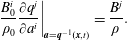 $$\begin{eqnarray}\left.\frac{B_{0}^{i}}{\unicode[STIX]{x1D70C}_{0}}\frac{\unicode[STIX]{x2202}q^{j}}{\unicode[STIX]{x2202}a^{i}}\right|_{\boldsymbol{a}=\boldsymbol{q}^{-1}(\boldsymbol{x},t)}=\frac{B^{j}}{\unicode[STIX]{x1D70C}}.\end{eqnarray}$$
Eulerianizing the counterpart of (3.45) for this expression gives
 $$\begin{eqnarray}\frac{\unicode[STIX]{x2202}}{\unicode[STIX]{x2202}t}\left(\frac{\boldsymbol{B}}{\unicode[STIX]{x1D70C}}\right)+\boldsymbol{v}\boldsymbol{\cdot }\unicode[STIX]{x1D735}\left(\frac{\boldsymbol{B}}{\unicode[STIX]{x1D70C}}\right)=\frac{\boldsymbol{B}}{\unicode[STIX]{x1D70C}}\boldsymbol{\cdot }\unicode[STIX]{x1D735}\boldsymbol{v},\end{eqnarray}$$
 which is not an Eulerian conservation law. This is to be expected because, unlike what we did to get (3.47), we have Eulerianized without using (3.42). In light of its relationship to  $\boldsymbol{q}(\boldsymbol{a},t)-\boldsymbol{q}(\boldsymbol{a}+\unicode[STIX]{x1D6FF}\boldsymbol{a},t)$, the quantity $\boldsymbol{B}/\unicode[STIX]{x1D70C}$ has been described as a measure of the distance of points on a magnetic field line (see e.g. Kampen & Felderhoff (Reference Van Kampen and Felderhoff1967)). This was predated by analogous arguments for vorticity (see e.g. Serrin (Reference Serrin and Flügge1959)).
4 Constraint theories for the incompressible ideal fluid
4.1 The incompressible fluid in Lagrangian variables
In order to enforce incompressibility, Lagrange added to his Lagrangian the constraint  ${\mathcal{J}}=1$ with the Lagrange multiplier $\unicode[STIX]{x1D706}(\boldsymbol{a},t)$,
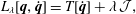 $$\begin{eqnarray}L_{\unicode[STIX]{x1D706}}[\boldsymbol{q},\dot{\boldsymbol{q}}]=T[\dot{\boldsymbol{q}}]+\unicode[STIX]{x1D706}\,{\mathcal{J}},\end{eqnarray}$$
 with  $T$ given (3.10). Here we have dropped $V$ because incompressible fluids contain no internal energy. Upon insertion of (4.1) into the action of Hamilton’s principle it is discovered that $\unicode[STIX]{x1D706}$ corresponds to the pressure. The essence of this procedure was known to Lagrange. (See Serrin (Reference Serrin and Flügge1959) for historical details and Sommerfeld (Reference Sommerfeld1964) for an elementary exposition.) This procedure yields
 $$\begin{eqnarray}\unicode[STIX]{x1D70C}_{0}\ddot{q}^{i}=-A_{j}^{i}\,\frac{\unicode[STIX]{x2202}\unicode[STIX]{x1D706}}{\unicode[STIX]{x2202}a^{j}},\end{eqnarray}$$
 where use has been made of (3.7). The Eulerian form of (4.2) is clearly  $\unicode[STIX]{x1D70C}(\unicode[STIX]{x2202}\boldsymbol{v}/\unicode[STIX]{x2202}t+\boldsymbol{v}\boldsymbol{\cdot }\unicode[STIX]{x1D735}\boldsymbol{v})=-\unicode[STIX]{x1D735}\unicode[STIX]{x1D706}$, whence it is clear that $\unicode[STIX]{x1D706}$ is the pressure. Although Lagrange knew the Lagrange multiplier was the pressure, he could only solve for it in special cases. The general procedure of § 1.1 was not available because Green’s function techniques and the theory of elliptic equations were not at his disposal.
4.1.1 Lagrangian volume preserving geodesic flow
If the constraint is dropped from (4.1), we obtain free particle motion for an infinite-dimensional system, the ideal fluid case of (2.80) of § 2.4, which is analogous to the finite-dimensional case of § 2.1.1. Because the constraint  ${\mathcal{J}}=1$ only depends on the derivatives of $\boldsymbol{q}$, it is a configuration space constraint; thus, it is an holonomic constraint. As is well known and reviewed in § 2.1.1, free particle motion with holonomic constaints is geodesic flow. Thus, following Lagrange, it is immediate that the ideal incompressible fluid is an infinite-dimensional version of geodesic flow.
Lagrange’s calculation was placed in a geometric/group theoretic setting in Arnold (Reference Arnold1966) (see also appendix 2 of Arnold (Reference Arnold1978) and Arnold & Khesin (Reference Arnold and Khesin1998)). Given that the transformation  $\boldsymbol{a}\leftrightarrow \boldsymbol{q}$, at any time, is assumed to be a smooth invertible coordinate change, it is a Lie group, one referred to as the diffeomorphism group. With the additional assumption that these transformations are volume preserving, Lagrange’s constraint ${\mathcal{J}}=1$, the transformations form a subgroup, the group of volume preserving diffeomorphisms. Thus, Lagrange’s work can be viewed as geodesic flow on the group of volume preserving diffeomorphisms.
Although Arnold’s assumptions of smoothness etc. are mathematically dramatic, his description of Lagrange’s calculations in these terms has spawned a considerable body of research. Associated with a geodesic flow is a metric, and whence one can calculate a curvature. In his original work, Arnold added the novel calculation of the curvature in the mathematically more forgiving case of two-dimensional flow with periodic boundary conditions.
4.2 Lagrangian–Dirac constraint theory
More recently there have been several works (Morrison et al. Reference Morrison, Lebovitz and Biello2009; Tassi et al. Reference Tassi, Chandre and Morrison2009; Chandre et al. Reference Chandre, de Guillebon, Back, Tassi and Morrison2013), following Nguyen & Turski (Reference Nguyen and Turski1999, Reference Nguyen and Turski2001), that treat the enforcement of the incompressibility constraint of hydrodynamics by Dirac’s method of constraints (Dirac Reference Dirac1950). In these works the compressibility constraint was enforced in the Eulerian variable description of the fluid using the noncanonical Poisson bracket of § 3.3 as the base bracket of a generalization of Dirac’s constraint theory. We will return to this approach in § 3.3 where we revisit and extend Dirac’s constraint results for the fluid in the Eulerian variable description. Here, apparently for the first time, we consider the incompressibility constraint in the Lagrangian variable description, where the canonical Poisson bracket of (3.15) is the base for the construction of a Dirac bracket.
We adapt (2.78) for the fluid case at hand with the supposition of only two local constraints, which we write as
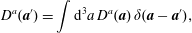 $$\begin{eqnarray}D^{a}(\boldsymbol{a}^{\prime })=\int \text{d}^{3}a\,D^{a}(\boldsymbol{a})\,\unicode[STIX]{x1D6FF}(\boldsymbol{a}-\boldsymbol{a}^{\prime }),\end{eqnarray}$$
 where  $a=1,2$ and $D^{a}(\boldsymbol{a})$ is a shorthand for a function of $\boldsymbol{q}(\boldsymbol{a},t)$ and $\unicode[STIX]{x03C0}(\boldsymbol{a},t)$ and their derivatives with respect to $\boldsymbol{a}$. Then the matrix $\mathbb{D}$ is a $2\times 2$ matrix with the components
 $$\begin{eqnarray}\mathbb{D}^{ab}(\boldsymbol{a},\boldsymbol{a}^{\prime })=\{D^{a}(\boldsymbol{a}),D^{b}(\boldsymbol{a}^{\prime })\},\end{eqnarray}$$
using the canonical bracket of (3.15). To construct the Dirac bracket
 $$\begin{eqnarray}\{F,G\}_{\ast }=\{F,G\}-\int \text{d}^{3}a\int \text{d}^{3}a^{\prime }\,\{F,D^{a}(\boldsymbol{a})\}\mathbb{D}_{ab}^{-1}(\boldsymbol{a},\boldsymbol{a}^{\prime })\{D^{b}(\boldsymbol{a}^{\prime }),G\},\end{eqnarray}$$
we require the inverse, which satisfies
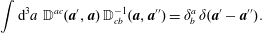 $$\begin{eqnarray}\int \text{d}^{3}a\,\,\mathbb{D}^{ac}(\boldsymbol{a}^{\prime },\boldsymbol{a})\,\mathbb{D}_{cb}^{-1}(\boldsymbol{a},\boldsymbol{a}^{\prime \prime })=\unicode[STIX]{x1D6FF}_{b}^{a}\,\unicode[STIX]{x1D6FF}(\boldsymbol{a}^{\prime }-\boldsymbol{a}^{\prime \prime }).\end{eqnarray}$$
Rather than continuing with the general case, which is unwieldy, we proceed to the special case for the incompressible fluid, an infinite-dimensional version of the holonomic constraints discussed in § 2.3.1.
4.2.1 Lagrangian–Dirac incompressibility holonomic constraint
Evidently we will want our holonomic incompressibility constraint to be  ${\mathcal{J}}$. However, it is convenient to express this by choosing
 $$\begin{eqnarray}D^{1}=\ln \left(\frac{{\mathcal{J}}}{\unicode[STIX]{x1D70C}_{0}}\right).\end{eqnarray}$$
 This amounts to the same constraint as  ${\mathcal{J}}=1$ with the value $D^{1}=-\ln (\unicode[STIX]{x1D70C}_{0})$. The scaling of ${\mathcal{J}}$ in (4.7) by $\unicode[STIX]{x1D70C}_{0}(\boldsymbol{a})$ is immaterial because it is a time-independent quantity. To obtain the second constraint we follow suit and set
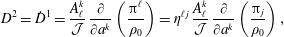 $$\begin{eqnarray}D^{2}={\dot{D}}^{1}=\frac{A_{\ell }^{k}}{{\mathcal{J}}}\,\frac{\unicode[STIX]{x2202}}{\unicode[STIX]{x2202}a^{k}}\left(\frac{\unicode[STIX]{x03C0}^{\ell }}{\unicode[STIX]{x1D70C}_{0}}\right)=\unicode[STIX]{x1D702}^{\ell j}\,\frac{A_{\ell }^{k}}{{\mathcal{J}}}\,\frac{\unicode[STIX]{x2202}}{\unicode[STIX]{x2202}a^{k}}\left(\frac{\unicode[STIX]{x03C0}_{j}}{\unicode[STIX]{x1D70C}_{0}}\right),\end{eqnarray}$$
 where recall we assume  $\unicode[STIX]{x1D702}^{\ell j}=\unicode[STIX]{x1D6FF}^{\ell j}$ and $\unicode[STIX]{x03C0}_{j}$ is given by (3.13). That the constraint $D^{2}$ is the time derivative of $D^{1}$ requires the definition of $\unicode[STIX]{x03C0}_{j}$ of (3.13) that uses the Hamiltonian $\int \text{d}^{3}a~|\unicode[STIX]{x03C0}|^{2}/(2\unicode[STIX]{x1D70C}_{0})$.
Observe, that constraints  $D^{1}$ and $D^{2}$ are local constraints in that they are enforced pointwise (see e.g. Flierl & Morrison (Reference Flierl and Morrison2011)), i.e. they are enforced on each fluid element labelled by $\boldsymbol{a}$. Equation (4.7) corresponds in the Eulerian picture to $-\ln (\unicode[STIX]{x1D70C})$, while the second constraint of (4.8), the Lagrangian time derivative of the first constraint, corresponds in the Eulerian picture to $\unicode[STIX]{x1D735}\boldsymbol{\cdot }\boldsymbol{v}$, which can be easily verified using the second equation of (3.35). Note, the particular values of these constraints of interest are, of course, ${\mathcal{J}}=1$ and $\unicode[STIX]{x1D735}\boldsymbol{\cdot }\boldsymbol{v}=0$, but the dynamics the Dirac bracket generates will preserve any values of these constraints. For example, we could set ${\mathcal{J}}=f(\boldsymbol{a})$ where the arbitrary function $f$ is less than unity for some $\boldsymbol{a}$ and greater for others, corresponding to regions of fluid elements that experience contraction and expansion. Also note, we have used $\unicode[STIX]{x03C0}$ with the up index in (4.8); thus as seen in the second equality it depends on the metric. This was done to make it have the Eulerian form $\unicode[STIX]{x1D735}\boldsymbol{\cdot }\boldsymbol{v}$.
For the constraints (4.7) and (4.8),  $\mathbb{D}$ only depends on two quantities because $D^{1}$ does not depend on $\unicode[STIX]{x03C0}$, i.e. $\{D^{1},D^{1}\}=0$ and $\{D^{1},D^{2}\}=-\{D^{2},D^{1}\}$. Thus the inverse has the form
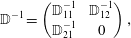 $$\begin{eqnarray}\mathbb{D}^{-1}=\left(\begin{array}{@{}cc@{}}\mathbb{D}_{11}^{-1} & \mathbb{D}_{12}^{-1}\\ \mathbb{ D}_{21}^{-1} & 0\end{array}\right),\end{eqnarray}$$
giving rise to the conditions
 $$\begin{eqnarray}\mathbb{D}_{12}^{-1}\boldsymbol{\cdot }\mathbb{D}^{21}={\mathcal{I}}=\mathbb{D}_{21}^{-1}\boldsymbol{\cdot }\mathbb{D}^{12}\,\quad \text{and}\quad \mathbb{D}_{11}^{-1}\boldsymbol{\cdot }\mathbb{D}^{12}+\mathbb{D}_{12}^{-1}\boldsymbol{\cdot }\mathbb{D}^{22}=0,\end{eqnarray}$$
 where  ${\mathcal{I}}$ is the identity. Thus, the inverse is easily tractable if the inverse of $\mathbb{D}^{12}$ exists; whence,
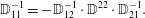 $$\begin{eqnarray}\mathbb{D}_{11}^{-1}=-\mathbb{D}_{12}^{-1}\cdot \mathbb{D}^{22}\cdot \mathbb{D}_{21}^{-1}.\end{eqnarray}$$
 In the above the symbol ‘ $\cdot$’ is used to denote the product with the sum in infinite dimensions, i.e. integration over $\text{d}^{3}a$ as in (4.6). Equation (4.11) can be rewritten in an abbreviated form with implied integrals on repeated arguments as
 $$\begin{eqnarray}\mathbb{D}_{11}^{-1}(\boldsymbol{a}^{\prime },\boldsymbol{a}^{\prime \prime })=\mathbb{D}_{21}^{-1}(\boldsymbol{a}^{\prime },\hat{\boldsymbol{a}})\boldsymbol{\cdot }\mathbb{D}^{22}(\hat{\boldsymbol{a}},\check{\boldsymbol{a}})\boldsymbol{\cdot }\mathbb{D}_{21}^{-1}(\check{\boldsymbol{a}},\boldsymbol{a}^{\prime \prime }).\end{eqnarray}$$
 In order to obtain  $\mathbb{D}$ and its inverse, we need the functional derivatives of $D^{1}$ and $D^{2}$. These are obtained directly by writing these local constraints as in (4.6), yielding
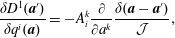 $$\begin{eqnarray}\displaystyle & \displaystyle \frac{\unicode[STIX]{x1D6FF}D^{1}(\boldsymbol{a}^{\prime })}{\unicode[STIX]{x1D6FF}q^{i}(\boldsymbol{a})}=-A_{i}^{k}\frac{\unicode[STIX]{x2202}}{\unicode[STIX]{x2202}a^{k}}\frac{\unicode[STIX]{x1D6FF}(\boldsymbol{a}-\boldsymbol{a}^{\prime })}{{\mathcal{J}}}, & \displaystyle\end{eqnarray}$$
 $$\begin{eqnarray}\displaystyle & \displaystyle \frac{\unicode[STIX]{x1D6FF}D^{1}(\boldsymbol{a}^{\prime })}{\unicode[STIX]{x1D6FF}\unicode[STIX]{x03C0}_{i}(\boldsymbol{a})}=0, & \displaystyle\end{eqnarray}$$
where use has been made of (3.7), and
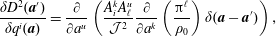 $$\begin{eqnarray}\displaystyle & \displaystyle \frac{\unicode[STIX]{x1D6FF}D^{2}(\boldsymbol{a}^{\prime })}{\unicode[STIX]{x1D6FF}q^{i}(\boldsymbol{a})}=\frac{\unicode[STIX]{x2202}}{\unicode[STIX]{x2202}a^{u}}\left(\frac{A_{i}^{k}A_{\ell }^{u}}{{\mathcal{J}}^{2}}\frac{\unicode[STIX]{x2202}}{\unicode[STIX]{x2202}a^{k}}\left(\frac{\unicode[STIX]{x03C0}^{\ell }}{\unicode[STIX]{x1D70C}_{0}}\right)\unicode[STIX]{x1D6FF}(\boldsymbol{a}-\boldsymbol{a}^{\prime })\right), & \displaystyle\end{eqnarray}$$
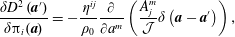 $$\begin{eqnarray}\displaystyle & \displaystyle \frac{\unicode[STIX]{x1D6FF}D^{2}\left(\boldsymbol{a}^{\prime }\right)}{\unicode[STIX]{x1D6FF}\unicode[STIX]{x03C0}_{i}(\boldsymbol{a})}=-\frac{\,\unicode[STIX]{x1D702}^{ij}}{\unicode[STIX]{x1D70C}_{0}}\frac{\unicode[STIX]{x2202}}{\unicode[STIX]{x2202}a^{m}}\left(\frac{A_{j}^{m}}{{\mathcal{J}}}\unicode[STIX]{x1D6FF}\left(\boldsymbol{a}-\boldsymbol{a}^{\prime }\right)\right), & \displaystyle\end{eqnarray}$$
where use has been made of (3.8) and recalling we have (3.6) at our disposal.
Let us now insert (4.13)–(4.16) into the canonical Poisson bracket (3.15), to obtain
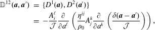 $$\begin{eqnarray}\displaystyle \mathbb{D}^{12}(\boldsymbol{a},\boldsymbol{a}^{\prime }) & = & \displaystyle \{D^{1}(\boldsymbol{a}),D^{2}(\boldsymbol{a}^{\prime })\}\nonumber\\ \displaystyle & = & \displaystyle -\frac{A_{i}^{\ell }}{{\mathcal{J}}}\frac{\unicode[STIX]{x2202}}{\unicode[STIX]{x2202}a^{\ell }}\left(\frac{\unicode[STIX]{x1D702}^{ij}}{\unicode[STIX]{x1D70C}_{0}}A_{j}^{k}\frac{\unicode[STIX]{x2202}}{\unicode[STIX]{x2202}a^{k}}\left(\frac{\unicode[STIX]{x1D6FF}(\boldsymbol{a}-\boldsymbol{a}^{\prime })}{{\mathcal{J}}}\right)\right),\end{eqnarray}$$
 which corresponds to the symmetric matrix  $\mathbb{S}$ of (2.27) and (2.42) and
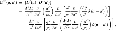 $$\begin{eqnarray}\displaystyle \mathbb{D}^{22}(\boldsymbol{a},\boldsymbol{a}^{\prime }) & = & \displaystyle \{D^{2}(\boldsymbol{a}),D^{2}(\boldsymbol{a}^{\prime })\}\nonumber\\ \displaystyle & = & \displaystyle \frac{A_{i}^{k}A_{\ell }^{u}}{{\mathcal{J}}^{2}}\frac{\unicode[STIX]{x2202}}{\unicode[STIX]{x2202}a^{k}}\left(\frac{\unicode[STIX]{x03C0}^{\ell }}{\unicode[STIX]{x1D70C}_{0}}\right)\frac{\unicode[STIX]{x2202}}{\unicode[STIX]{x2202}a^{u}}\left[\frac{\unicode[STIX]{x1D702}^{ij}}{\unicode[STIX]{x1D70C}_{0}}\frac{\unicode[STIX]{x2202}}{\unicode[STIX]{x2202}a^{m}}\left(\frac{A_{j}^{m}}{{\mathcal{J}}}\unicode[STIX]{x1D6FF}\left(\boldsymbol{a}-\boldsymbol{a}^{\prime }\right)\right)\right]\nonumber\\ \displaystyle & & \displaystyle -\,\frac{A_{i}^{m}}{{\mathcal{J}}}\frac{\unicode[STIX]{x2202}}{\unicode[STIX]{x2202}a^{m}}\left[\frac{\unicode[STIX]{x1D702}^{ij}}{\unicode[STIX]{x1D70C}_{0}}\frac{\unicode[STIX]{x2202}}{\unicode[STIX]{x2202}a^{u}}\left(\frac{A_{j}^{k}A_{\ell }^{u}}{{\mathcal{J}}^{2}}\frac{\unicode[STIX]{x2202}}{\unicode[STIX]{x2202}a^{k}}\left(\frac{\unicode[STIX]{x03C0}^{\ell }}{\unicode[STIX]{x1D70C}_{0}}\right)\unicode[STIX]{x1D6FF}(\boldsymbol{a}-\boldsymbol{a}^{\prime })\right)\right],\end{eqnarray}$$
 which corresponds to the antisymmetric matrix  $\mathbb{A}$ of (2.28). Observe the symmetries corresponding to the matrices $\mathbb{S}$ and $\mathbb{A}$, respectively, are here
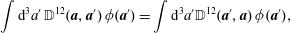 $$\begin{eqnarray}\displaystyle & \displaystyle \int \text{d}^{3}a^{\prime }\,\mathbb{D}^{12}(\boldsymbol{a},\boldsymbol{a}^{\prime })\,\unicode[STIX]{x1D719}(\boldsymbol{a}^{\prime })=\int \text{d}^{3}a^{\prime }\mathbb{D}^{12}(\boldsymbol{a}^{\prime },\boldsymbol{a})\,\unicode[STIX]{x1D719}(\boldsymbol{a}^{\prime }), & \displaystyle\end{eqnarray}$$
 $$\begin{eqnarray}\displaystyle & \displaystyle \int \text{d}^{3}a^{\prime }\,\mathbb{D}^{22}(\boldsymbol{a},\boldsymbol{a}^{\prime })\,\unicode[STIX]{x1D719}(\boldsymbol{a}^{\prime })=-\int \text{d}^{3}a^{\prime }\mathbb{D}^{22}(\boldsymbol{a}^{\prime },\boldsymbol{a})\,\unicode[STIX]{x1D719}(\boldsymbol{a}^{\prime }), & \displaystyle\end{eqnarray}$$
 for all functions  $\unicode[STIX]{x1D719}$. The first follows from integration by parts, while the second is obvious from its definition.
Using (4.6), the first condition of (4.10) is
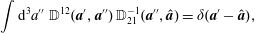 $$\begin{eqnarray}\int \text{d}^{3}a^{\prime \prime }\,\,\mathbb{D}^{12}(\boldsymbol{a}^{\prime },\boldsymbol{a}^{\prime \prime })\,\mathbb{D}_{21}^{-1}(\boldsymbol{a}^{\prime \prime },\hat{\boldsymbol{a}})=\unicode[STIX]{x1D6FF}(\boldsymbol{a}^{\prime }-\hat{\boldsymbol{a}}),\end{eqnarray}$$
which upon substitution of (4.17) and integration gives
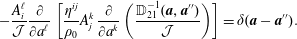 $$\begin{eqnarray}-\frac{A_{i}^{\ell }}{{\mathcal{J}}}\frac{\unicode[STIX]{x2202}}{\unicode[STIX]{x2202}a^{\ell }}\left[\frac{\unicode[STIX]{x1D702}^{ij}}{\unicode[STIX]{x1D70C}_{0}}A_{j}^{k}\,\frac{\unicode[STIX]{x2202}}{\unicode[STIX]{x2202}a^{k}}\left(\frac{\mathbb{D}_{21}^{-1}(\boldsymbol{a},\boldsymbol{a}^{\prime \prime })}{{\mathcal{J}}}\right)\right]=\unicode[STIX]{x1D6FF}(\boldsymbol{a}-\boldsymbol{a}^{\prime \prime }).\end{eqnarray}$$
We introduce the formally self-adjoint operator (cf. (3.6))
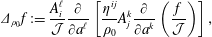 $$\begin{eqnarray}\unicode[STIX]{x1D6E5}_{\unicode[STIX]{x1D70C}_{0}}f:=\frac{A_{i}^{\ell }}{{\mathcal{J}}}\frac{\unicode[STIX]{x2202}}{\unicode[STIX]{x2202}a^{\ell }}\left[\frac{\unicode[STIX]{x1D702}^{ij}}{\unicode[STIX]{x1D70C}_{0}}A_{j}^{k}\frac{\unicode[STIX]{x2202}}{\unicode[STIX]{x2202}a^{k}}\left(\frac{f}{{\mathcal{J}}}\right)\right],\end{eqnarray}$$
i.e. an operator that satisfies
 $$\begin{eqnarray}\int \text{d}^{3}a\,f(\boldsymbol{a})\,\unicode[STIX]{x1D6E5}_{\unicode[STIX]{x1D70C}_{0}}g(\boldsymbol{a})=\int \text{d}^{3}a\,g(\boldsymbol{a})\,\unicode[STIX]{x1D6E5}_{\unicode[STIX]{x1D70C}_{0}}f(\boldsymbol{a}),\end{eqnarray}$$
 a property inherited by its inverse  $\unicode[STIX]{x1D6E5}_{\unicode[STIX]{x1D70C}_{0}}^{-1}$. Thus we can rewrite equation (4.22) as
 $$\begin{eqnarray}\mathbb{D}_{21}^{-1}(\boldsymbol{a},\boldsymbol{a}^{\prime \prime })=-G_{0}\left(\boldsymbol{a},\boldsymbol{a}^{\prime \prime }\right)=-\unicode[STIX]{x1D6E5}_{\unicode[STIX]{x1D70C}_{0}}^{-1}\unicode[STIX]{x1D6FF}(\boldsymbol{a}-\boldsymbol{a}^{\prime \prime }),\end{eqnarray}$$
 where  $G_{0}$ represents the Green function associated with (4.22).
In order to obtain  $\mathbb{D}_{21}^{-1}$, we find it convenient to transform (4.25) to Eulerian variables. Using $\boldsymbol{x}=\boldsymbol{q}(\boldsymbol{a},t)$ we find
 $$\begin{eqnarray}\frac{\mathbb{D}_{21}^{-1}(\boldsymbol{a},\boldsymbol{a}^{\prime })}{{\mathcal{J}}}=-G(\boldsymbol{x},\boldsymbol{x}^{\prime })=-G(\boldsymbol{q}(\boldsymbol{a}),\boldsymbol{q}(\boldsymbol{a}^{\prime })),\end{eqnarray}$$
 where  $G$ satisfies
 $$\begin{eqnarray}\unicode[STIX]{x1D735}\boldsymbol{\cdot }\left(\frac{1}{\unicode[STIX]{x1D70C}}\unicode[STIX]{x1D735}G\right)=-\unicode[STIX]{x1D6E5}_{\unicode[STIX]{x1D70C}}\frac{\mathbb{D}_{21}^{-1}(\boldsymbol{a},\boldsymbol{a}^{\prime })}{{\mathcal{J}}}={\mathcal{J}}\unicode[STIX]{x1D6FF}(\boldsymbol{x}-\boldsymbol{x}^{\prime }).\end{eqnarray}$$
Here use has been made of identities (3.6) and (3.35). As noted in § 1.1, under physically reasonable conditions, the operator
 $$\begin{eqnarray}\unicode[STIX]{x1D6E5}_{\unicode[STIX]{x1D70C}}f=\unicode[STIX]{x1D6E5}_{\unicode[STIX]{x1D70C}_{0}}({\mathcal{J}}f)=\unicode[STIX]{x1D735}\boldsymbol{\cdot }\left(\frac{1}{\unicode[STIX]{x1D70C}}\unicode[STIX]{x1D735}f\right)\end{eqnarray}$$
has an inverse. Thus we write
 $$\begin{eqnarray}\mathbb{D}_{21}^{-1}(\boldsymbol{a},\boldsymbol{a}^{\prime })=-{\mathcal{J}}\unicode[STIX]{x1D6E5}_{\unicode[STIX]{x1D70C}}^{-1}\Big({\mathcal{J}}\,\unicode[STIX]{x1D6FF}\big(\boldsymbol{q}(\boldsymbol{a},t)-\boldsymbol{q}(\boldsymbol{a}^{\prime },t)\big)\Big).\end{eqnarray}$$
 Now, using  $\mathbb{D}_{21}^{-1}=-\mathbb{D}_{12}^{-1}$, the element $\mathbb{D}_{11}^{-1}$ follows directly from (4.11).
For convenience we write the Dirac bracket of (4.5) as follows:
 $$\begin{eqnarray}\{F,G\}_{\ast }=\{F,G\}-[F,G]^{D},\end{eqnarray}$$
where
 $$\begin{eqnarray}\displaystyle [F,G]^{D}:=\mathop{\sum }_{a,b=1}^{2}[F,G]_{ab}^{D}=\int \text{d}^{3}a\,\int \text{d}^{3}a^{\prime }\,\,\left\{F,D^{a}(\boldsymbol{a})\right\}\mathbb{D}_{ab}^{-1}(\boldsymbol{a},\boldsymbol{a}^{\prime })\{D^{b}(\boldsymbol{a}^{\prime }),G\}. & & \displaystyle\end{eqnarray}$$
 Because  $\mathbb{D}_{22}^{-1}=0$ and $[F,G]_{12}^{D}=-[G,F]_{21}^{D}$, we only need to calculate $[F,G]_{11}^{D}$ and $[F,G]_{21}^{D}$.
As above, we substitute (4.13), (4.14), (4.15), and (4.16) into the bracket (3.15) and obtain
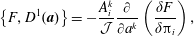 $$\begin{eqnarray}\displaystyle & \displaystyle \left\{F,D^{1}(\boldsymbol{a})\right\}=-\frac{A_{i}^{k}}{{\mathcal{J}}}\frac{\unicode[STIX]{x2202}}{\unicode[STIX]{x2202}a^{k}}\left(\frac{\unicode[STIX]{x1D6FF}F}{\unicode[STIX]{x1D6FF}\unicode[STIX]{x03C0}_{i}}\right), & \displaystyle\end{eqnarray}$$
 $$\begin{eqnarray}\displaystyle & \displaystyle \left\{F,D^{2}(\boldsymbol{a})\right\}=\frac{A_{\ell }^{k}}{{\mathcal{J}}}\frac{\unicode[STIX]{x2202}}{\unicode[STIX]{x2202}a^{k}}\left(\frac{\unicode[STIX]{x1D702}^{i\ell }}{\unicode[STIX]{x1D70C}_{0}}\frac{\unicode[STIX]{x1D6FF}F}{\unicode[STIX]{x1D6FF}q^{i}}\right)+\frac{A_{i}^{k}}{{\mathcal{J}}}\frac{A_{\ell }^{u}}{{\mathcal{J}}}\frac{\unicode[STIX]{x2202}}{\unicode[STIX]{x2202}a^{k}}\left(\frac{\unicode[STIX]{x03C0}^{\ell }}{\unicode[STIX]{x1D70C}_{0}}\right)\,\frac{\unicode[STIX]{x2202}}{\unicode[STIX]{x2202}a^{u}}\left(\frac{\unicode[STIX]{x1D6FF}F}{\unicode[STIX]{x1D6FF}\unicode[STIX]{x03C0}_{i}}\right). & \displaystyle\end{eqnarray}$$
 Then, exploiting the antisymmetry of the Poisson bracket, it is straightforward to calculate analogous expressions for the terms  $\{D^{1,2},G\}$.
We first analyse the operator
 $$\begin{eqnarray}[F,G]_{11}^{D}=\!\int \!\text{d}^{3}a\!\int \!\text{d}^{3}a^{\prime }\!\int \!\text{d}^{3}\hat{a}\!\int \!\text{d}^{3}{\check{a}}\{F,D^{1}(\boldsymbol{a})\}\mathbb{D}_{21}^{-1}(\boldsymbol{a},\hat{\boldsymbol{a}})\mathbb{D}^{22}(\hat{\boldsymbol{a}},\check{\boldsymbol{a}})\,\mathbb{D}_{21}^{-1}(\check{\boldsymbol{a}},\boldsymbol{a}^{\prime })\{D^{1}(\boldsymbol{a}^{\prime }),G\},\end{eqnarray}$$
 where we used the second condition of (4.10) to replace  $\mathbb{D}_{11}^{-1}$. Upon inserting (4.25) and (4.32), this equation can be rewritten as
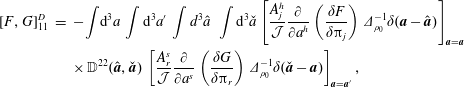 $$\begin{eqnarray}\displaystyle [F,G]_{11}^{D} & = & \displaystyle -\int \text{d}^{3}a\,\int \text{d}^{3}a^{\prime }\,\int d^{3}\hat{a}\,\,\int \text{d}^{3}{\check{a}}\left[\frac{A_{j}^{h}}{{\mathcal{J}}}\frac{\unicode[STIX]{x2202}}{\unicode[STIX]{x2202}a^{h}}\left(\frac{\unicode[STIX]{x1D6FF}F}{\unicode[STIX]{x1D6FF}\unicode[STIX]{x03C0}_{j}}\right)\unicode[STIX]{x1D6E5}_{\unicode[STIX]{x1D70C}_{0}}^{-1}\unicode[STIX]{x1D6FF}(\boldsymbol{a}-\hat{\boldsymbol{a}})\right]_{\boldsymbol{a}=\boldsymbol{a}}\nonumber\\ \displaystyle & & \displaystyle \times \,\mathbb{D}^{22}(\hat{\boldsymbol{a}},\check{\boldsymbol{a}})\,\left[\frac{A_{r}^{s}}{{\mathcal{J}}}\frac{\unicode[STIX]{x2202}}{\unicode[STIX]{x2202}a^{s}}\left(\frac{\unicode[STIX]{x1D6FF}G}{\unicode[STIX]{x1D6FF}\unicode[STIX]{x03C0}_{r}}\right)\unicode[STIX]{x1D6E5}_{\unicode[STIX]{x1D70C}_{0}}^{-1}\unicode[STIX]{x1D6FF}(\check{\boldsymbol{a}}-\boldsymbol{a})\right]_{\boldsymbol{a}=\boldsymbol{a}^{\prime }},\end{eqnarray}$$
 where the subscripts on the right delimiters indicate that  $\boldsymbol{a}$ is to be replaced after the derivative operations, including those that occur in ${\mathcal{J}}$ and $A_{i}^{j}$.
Integrating this expression by parts with respect to  $\boldsymbol{a}$ and $\boldsymbol{a}^{\prime }$ yields
 $$\begin{eqnarray}\displaystyle [F,G]_{11}^{D} & = & \displaystyle -\int \text{d}^{3}\hat{a}\,\,\int \text{d}^{3}{\check{a}}\,\,\left[\unicode[STIX]{x1D6E5}_{\unicode[STIX]{x1D70C}_{0}}^{-1}\left(\frac{A_{j}^{h}}{{\mathcal{J}}}\frac{\unicode[STIX]{x2202}}{\unicode[STIX]{x2202}a^{h}}\left(\frac{\unicode[STIX]{x1D6FF}F}{\unicode[STIX]{x1D6FF}\unicode[STIX]{x03C0}_{j}}\right)\right)\right]_{\boldsymbol{a}=\hat{\boldsymbol{a}}}\nonumber\\ \displaystyle & & \displaystyle \times \,\mathbb{D}^{22}(\hat{\boldsymbol{a}},\check{\boldsymbol{a}})\,\left[\unicode[STIX]{x1D6E5}_{\unicode[STIX]{x1D70C}_{0}}^{-1}\left(\frac{A_{r}^{s}}{{\mathcal{J}}}\frac{\unicode[STIX]{x2202}}{\unicode[STIX]{x2202}a^{s}}\left(\frac{\unicode[STIX]{x1D6FF}G}{\unicode[STIX]{x1D6FF}\unicode[STIX]{x03C0}_{r}}\right)\right)\right]_{\boldsymbol{a}=\check{\boldsymbol{a}}},\end{eqnarray}$$
and then substituting (4.18) gives
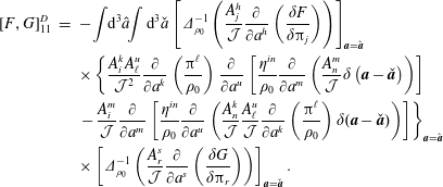 $$\begin{eqnarray}\displaystyle [F,G]_{11}^{D} & = & \displaystyle -\int \text{d}^{3}\hat{a}\!\!\int \text{d}^{3}{\check{a}}\left[\unicode[STIX]{x1D6E5}_{\unicode[STIX]{x1D70C}_{0}}^{-1}\left(\frac{A_{j}^{h}}{{\mathcal{J}}}\frac{\unicode[STIX]{x2202}}{\unicode[STIX]{x2202}a^{h}}\left(\frac{\unicode[STIX]{x1D6FF}F}{\unicode[STIX]{x1D6FF}\unicode[STIX]{x03C0}_{j}}\right)\right)\right]_{\boldsymbol{a}=\hat{\boldsymbol{a}}}\nonumber\\ \displaystyle & & \displaystyle \times \left\{\frac{A_{i}^{k}A_{\ell }^{u}}{{\mathcal{J}}^{2}}\frac{\unicode[STIX]{x2202}}{\unicode[STIX]{x2202}a^{k}}\left(\frac{\unicode[STIX]{x03C0}^{\ell }}{\unicode[STIX]{x1D70C}_{0}}\right)\frac{\unicode[STIX]{x2202}}{\unicode[STIX]{x2202}a^{u}}\left[\frac{\unicode[STIX]{x1D702}^{in}}{\unicode[STIX]{x1D70C}_{0}}\frac{\unicode[STIX]{x2202}}{\unicode[STIX]{x2202}a^{m}}\left(\frac{A_{n}^{m}}{{\mathcal{J}}}\unicode[STIX]{x1D6FF}\left(\boldsymbol{a}-\check{\boldsymbol{a}}\right)\right)\right]\right.\nonumber\\ \displaystyle & & \displaystyle \left.-\,\frac{A_{i}^{m}}{{\mathcal{J}}}\frac{\unicode[STIX]{x2202}}{\unicode[STIX]{x2202}a^{m}}\left[\frac{\unicode[STIX]{x1D702}^{in}}{\unicode[STIX]{x1D70C}_{0}}\frac{\unicode[STIX]{x2202}}{\unicode[STIX]{x2202}a^{u}}\left(\frac{A_{n}^{k}}{{\mathcal{J}}}\frac{A_{\ell }^{u}}{{\mathcal{J}}}\frac{\unicode[STIX]{x2202}}{\unicode[STIX]{x2202}a^{k}}\left(\frac{\unicode[STIX]{x03C0}^{\ell }}{\unicode[STIX]{x1D70C}_{0}}\right)\unicode[STIX]{x1D6FF}(\boldsymbol{a}-\check{\boldsymbol{a}})\right)\right]\right\}_{\boldsymbol{a}=\hat{\boldsymbol{a}}}\nonumber\\ \displaystyle & & \displaystyle \times \left[\unicode[STIX]{x1D6E5}_{\unicode[STIX]{x1D70C}_{0}}^{-1}\left(\frac{A_{r}^{s}}{{\mathcal{J}}}\frac{\unicode[STIX]{x2202}}{\unicode[STIX]{x2202}a^{s}}\left(\frac{\unicode[STIX]{x1D6FF}G}{\unicode[STIX]{x1D6FF}\unicode[STIX]{x03C0}_{r}}\right)\right)\right]_{\boldsymbol{a}=\check{\boldsymbol{a}}}.\end{eqnarray}$$
 Then, by means of integrations by parts we can remove the derivatives from the term  $\unicode[STIX]{x1D6FF}(\boldsymbol{a}-\check{\boldsymbol{a}})$ and perform the integral. After relabelling the integration variable as $\boldsymbol{a}$ to simplify the notation, equation (4.37) becomes
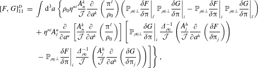 $$\begin{eqnarray}\displaystyle [F,G]_{11}^{D} & = & \displaystyle \int \text{d}^{3}a\left\{\unicode[STIX]{x1D70C}_{0}\unicode[STIX]{x1D702}^{ui}\frac{A_{u}^{k}}{{\mathcal{J}}}\frac{\unicode[STIX]{x2202}}{\unicode[STIX]{x2202}a^{k}}\left(\frac{\unicode[STIX]{x03C0}^{\ell }}{\unicode[STIX]{x1D70C}_{0}}\right)\!\left(\left.\mathbb{P}_{\unicode[STIX]{x1D70C}_{0}\bot }\frac{\unicode[STIX]{x1D6FF}F}{\unicode[STIX]{x1D6FF}\unicode[STIX]{x03C0}}\right|_{\ell }\left.\mathbb{P}_{\unicode[STIX]{x1D70C}_{0}\bot }\frac{\unicode[STIX]{x1D6FF}G}{\unicode[STIX]{x1D6FF}\unicode[STIX]{x03C0}}\right|_{i}-\left.\mathbb{P}_{\unicode[STIX]{x1D70C}_{0}\bot }\frac{\unicode[STIX]{x1D6FF}F}{\unicode[STIX]{x1D6FF}\unicode[STIX]{x03C0}}\right|_{i}\left.\mathbb{P}_{\unicode[STIX]{x1D70C}_{0}\bot }\frac{\unicode[STIX]{x1D6FF}G}{\unicode[STIX]{x1D6FF}\unicode[STIX]{x03C0}}\right|_{\ell }\right)\right.\nonumber\\ \displaystyle & & \displaystyle +\,\unicode[STIX]{x1D702}^{ni}A_{\ell }^{u}\frac{\unicode[STIX]{x2202}}{\unicode[STIX]{x2202}a^{u}}\left[\frac{A_{n}^{k}}{{\mathcal{J}}}\frac{\unicode[STIX]{x2202}}{\unicode[STIX]{x2202}a^{k}}\left(\frac{\unicode[STIX]{x03C0}^{\ell }}{\unicode[STIX]{x1D70C}_{0}}\right)\right]\left[\left.\mathbb{P}_{\unicode[STIX]{x1D70C}_{0}\bot }\frac{\unicode[STIX]{x1D6FF}G}{\unicode[STIX]{x1D6FF}\unicode[STIX]{x03C0}}\right|_{i}\frac{\unicode[STIX]{x1D6E5}_{\unicode[STIX]{x1D70C}_{0}}^{-1}}{{\mathcal{J}}}\left(\frac{A_{j}^{h}}{{\mathcal{J}}}\frac{\unicode[STIX]{x2202}}{\unicode[STIX]{x2202}a^{h}}\left(\frac{\unicode[STIX]{x1D6FF}F}{\unicode[STIX]{x1D6FF}\unicode[STIX]{x03C0}_{j}}\right)\right)\right.\nonumber\\ \displaystyle & & \displaystyle \left.\left.-\left.\mathbb{P}_{\unicode[STIX]{x1D70C}_{0}\bot }\frac{\unicode[STIX]{x1D6FF}F}{\unicode[STIX]{x1D6FF}\unicode[STIX]{x03C0}}\right|_{i}\frac{\unicode[STIX]{x1D6E5}_{\unicode[STIX]{x1D70C}_{0}}^{-1}}{{\mathcal{J}}}\left(\frac{A_{j}^{h}}{{\mathcal{J}}}\frac{\unicode[STIX]{x2202}}{\unicode[STIX]{x2202}a^{h}}\left(\frac{\unicode[STIX]{x1D6FF}G}{\unicode[STIX]{x1D6FF}\unicode[STIX]{x03C0}_{j}}\right)\right)\right]\right\},\end{eqnarray}$$
where we introduced the projection operator
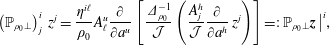 $$\begin{eqnarray}\left(\mathbb{P}_{\unicode[STIX]{x1D70C}_{0}\bot }\right)_{j}^{i}\,z^{j}=\frac{\unicode[STIX]{x1D702}^{i\ell }}{\unicode[STIX]{x1D70C}_{0}}A_{\ell }^{u}\frac{\unicode[STIX]{x2202}}{\unicode[STIX]{x2202}a^{u}}\left[\frac{\unicode[STIX]{x1D6E5}_{\unicode[STIX]{x1D70C}_{0}}^{-1}}{{\mathcal{J}}}\left(\frac{A_{j}^{h}}{{\mathcal{J}}}\frac{\unicode[STIX]{x2202}}{\unicode[STIX]{x2202}a^{h}}\,z^{j}\right)\right]=:\mathbb{P}_{\unicode[STIX]{x1D70C}_{0}\bot }\boldsymbol{z}\,\big|^{i},\end{eqnarray}$$
where in the last equality we defined a shorthand for convenience; thus,
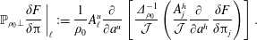 $$\begin{eqnarray}\left.\mathbb{P}_{\unicode[STIX]{x1D70C}_{0}\bot }\frac{\unicode[STIX]{x1D6FF}F}{\unicode[STIX]{x1D6FF}\unicode[STIX]{x03C0}}\,\right|_{\ell }:=\frac{1}{\unicode[STIX]{x1D70C}_{0}}A_{\ell }^{u}\frac{\unicode[STIX]{x2202}}{\unicode[STIX]{x2202}a^{u}}\left[\frac{\unicode[STIX]{x1D6E5}_{\unicode[STIX]{x1D70C}_{0}}^{-1}}{{\mathcal{J}}}\left(\frac{A_{j}^{h}}{{\mathcal{J}}}\frac{\unicode[STIX]{x2202}}{\unicode[STIX]{x2202}a^{h}}\,\frac{\unicode[STIX]{x1D6FF}F}{\unicode[STIX]{x1D6FF}\unicode[STIX]{x03C0}_{j}}\right)\right].\end{eqnarray}$$
 It is straightforward to prove that  $\mathbb{P}_{\unicode[STIX]{x1D70C}_{0}\bot }$ represents a projection, i.e. $\mathbb{P}_{\unicode[STIX]{x1D70C}_{0}\bot }(\mathbb{P}_{\unicode[STIX]{x1D70C}_{0}\bot }\boldsymbol{z})=\mathbb{P}_{\unicode[STIX]{x1D70C}_{0}\bot }\boldsymbol{z}$ for each $\boldsymbol{z}$, which in terms of indices would have an $i$th component given by $(\mathbb{P}_{\unicode[STIX]{x1D70C}_{0}\bot })_{j}^{i}(\mathbb{P}_{\unicode[STIX]{x1D70C}_{0}\bot })_{k}^{j}\,z^{k}=(\mathbb{P}_{\unicode[STIX]{x1D70C}_{0}\bot })_{k}^{i}\,z^{k}$. Also, $\mathbb{P}_{\unicode[STIX]{x1D70C}_{0}\bot }$ is formally self-adjoint with respect to the following weighted inner product:
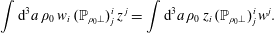 $$\begin{eqnarray}\int \text{d}^{3}a\,\unicode[STIX]{x1D70C}_{0}\,w_{i}\,(\mathbb{P}_{\unicode[STIX]{x1D70C}_{0}\bot })_{j}^{i}\,z\,^{j}=\int \text{d}^{3}a\,\unicode[STIX]{x1D70C}_{0}\,z_{i}\,(\mathbb{P}_{\unicode[STIX]{x1D70C}_{0}\bot })_{j}^{i}\,w^{j}.\end{eqnarray}$$
 The projection operator complementary to  $\mathbb{P}_{\unicode[STIX]{x1D70C}_{0}\bot }$ is given by
 $$\begin{eqnarray}\mathbb{P}_{\unicode[STIX]{x1D70C}_{0}}=\unicode[STIX]{x1D644}-\mathbb{P}_{\unicode[STIX]{x1D70C}_{0}\bot },\end{eqnarray}$$
 where  $\unicode[STIX]{x1D644}$ is the identity.
Now let us return to our evaluation of  $[F,G]_{D}$ and analyse the contribution
 $$\begin{eqnarray}\displaystyle [F,G]_{21}^{D}=\int \text{d}^{3}a\,\int \text{d}^{3}a^{\prime }\,\,\left\{F,D^{2}(\boldsymbol{a})\right\}\mathbb{D}_{21}^{-1}(\boldsymbol{a},\boldsymbol{a}^{\prime })\left\{D^{1}(\boldsymbol{a}^{\prime }),G\right\}. & & \displaystyle\end{eqnarray}$$
Using (4.29), (4.32) and (4.33), this equation can be rewritten as
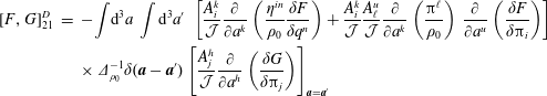 $$\begin{eqnarray}\displaystyle [F,G]_{21}^{D} & = & \displaystyle -\int \text{d}^{3}a\,\int \text{d}^{3}a^{\prime }\,\,\left[\frac{A_{i}^{k}}{{\mathcal{J}}}\frac{\unicode[STIX]{x2202}}{\unicode[STIX]{x2202}a^{k}}\left(\frac{\unicode[STIX]{x1D702}^{in}}{\unicode[STIX]{x1D70C}_{0}}\frac{\unicode[STIX]{x1D6FF}F}{\unicode[STIX]{x1D6FF}q^{n}}\right)+\frac{A_{i}^{k}}{{\mathcal{J}}}\frac{A_{\ell }^{u}}{{\mathcal{J}}}\frac{\unicode[STIX]{x2202}}{\unicode[STIX]{x2202}a^{k}}\left(\frac{\unicode[STIX]{x03C0}^{\ell }}{\unicode[STIX]{x1D70C}_{0}}\right)\,\frac{\unicode[STIX]{x2202}}{\unicode[STIX]{x2202}a^{u}}\left(\frac{\unicode[STIX]{x1D6FF}F}{\unicode[STIX]{x1D6FF}\unicode[STIX]{x03C0}_{i}}\right)\right]\nonumber\\ \displaystyle & & \displaystyle \times \,\unicode[STIX]{x1D6E5}_{\unicode[STIX]{x1D70C}_{0}}^{-1}\unicode[STIX]{x1D6FF}(\boldsymbol{a}-\boldsymbol{a}^{\prime })\left[\frac{A_{j}^{h}}{{\mathcal{J}}}\frac{\unicode[STIX]{x2202}}{\unicode[STIX]{x2202}a^{h}}\left(\frac{\unicode[STIX]{x1D6FF}G}{\unicode[STIX]{x1D6FF}\unicode[STIX]{x03C0}_{j}}\right)\right]_{\boldsymbol{a}=\boldsymbol{a}^{\prime }}\end{eqnarray}$$
 and, integrating by parts to simplify the  $\unicode[STIX]{x1D6FF}(\boldsymbol{a}-\boldsymbol{a}^{\prime })$ term, results in
 $$\begin{eqnarray}\displaystyle [F,G]_{21}^{D} & = & \displaystyle \int \text{d}^{3}a\,\,\left\{\frac{\unicode[STIX]{x1D6FF}F}{\unicode[STIX]{x1D6FF}q^{i}}\left.\mathbb{P}_{\unicode[STIX]{x1D70C}_{0}\bot }\frac{\unicode[STIX]{x1D6FF}G}{\unicode[STIX]{x1D6FF}\unicode[STIX]{x03C0}}\right|^{i}+\unicode[STIX]{x1D70C}_{0}\frac{A_{i}^{k}}{{\mathcal{J}}}\frac{\unicode[STIX]{x2202}}{\unicode[STIX]{x2202}a^{k}}\left(\frac{\unicode[STIX]{x03C0}^{\ell }}{\unicode[STIX]{x1D70C}_{0}}\right)\,\frac{\unicode[STIX]{x1D6FF}F}{\unicode[STIX]{x1D6FF}\unicode[STIX]{x03C0}_{i}}\left.\mathbb{P}_{\unicode[STIX]{x1D70C}_{0}\bot }\frac{\unicode[STIX]{x1D6FF}G}{\unicode[STIX]{x1D6FF}\unicode[STIX]{x03C0}}\right|_{\ell }\right.\nonumber\\ \displaystyle & & \displaystyle \left.+\,A_{\ell }^{u}\frac{\unicode[STIX]{x2202}}{\unicode[STIX]{x2202}a^{u}}\left[\frac{A_{i}^{k}}{{\mathcal{J}}}\frac{\unicode[STIX]{x2202}}{\unicode[STIX]{x2202}a^{k}}\left(\frac{\unicode[STIX]{x03C0}^{\ell }}{\unicode[STIX]{x1D70C}_{0}}\right)\right]\,\frac{\unicode[STIX]{x1D6FF}F}{\unicode[STIX]{x1D6FF}\unicode[STIX]{x03C0}_{i}}\frac{\unicode[STIX]{x1D6E5}_{\unicode[STIX]{x1D70C}_{0}}^{-1}}{{\mathcal{J}}}\left(\frac{A_{j}^{h}}{{\mathcal{J}}}\frac{\unicode[STIX]{x2202}}{\unicode[STIX]{x2202}a^{h}}\left(\frac{\unicode[STIX]{x1D6FF}G}{\unicode[STIX]{x1D6FF}\unicode[STIX]{x03C0}_{j}}\right)\right)\right\}.\end{eqnarray}$$
 We can now combine the operators  $[F,G]_{11}^{D}$, $[F,G]_{21}^{D}$, and $[F,G]_{12}^{D}=-[G,F]_{21}^{D}$, given by (4.38) and (4.45), to calculate the Dirac bracket (4.30). First, we rewrite (4.31) as
 $$\begin{eqnarray}\displaystyle [F,G]^{D} & = & \displaystyle \int \text{d}^{3}a\,\,\left\{\frac{\unicode[STIX]{x1D6FF}F}{\unicode[STIX]{x1D6FF}q^{i}}\left.\mathbb{P}_{\unicode[STIX]{x1D70C}_{0}\bot }\frac{\unicode[STIX]{x1D6FF}G}{\unicode[STIX]{x1D6FF}\unicode[STIX]{x03C0}}\right|^{i}-\frac{\unicode[STIX]{x1D6FF}G}{\unicode[STIX]{x1D6FF}q^{i}}\left.\mathbb{P}_{\unicode[STIX]{x1D70C}_{0}\bot }\frac{\unicode[STIX]{x1D6FF}F}{\unicode[STIX]{x1D6FF}\unicode[STIX]{x03C0}}\right|^{i}\right.\nonumber\\ \displaystyle & & \displaystyle +\,\unicode[STIX]{x1D70C}_{0}\frac{A_{i}^{k}}{{\mathcal{J}}}\frac{\unicode[STIX]{x2202}}{\unicode[STIX]{x2202}a^{k}}\left(\frac{\unicode[STIX]{x03C0}^{\ell }}{\unicode[STIX]{x1D70C}_{0}}\right)\,\left(\left.\mathbb{P}_{\unicode[STIX]{x1D70C}_{0}}\frac{\unicode[STIX]{x1D6FF}F}{\unicode[STIX]{x1D6FF}\unicode[STIX]{x03C0}}\right|^{i}\left.\mathbb{P}_{\unicode[STIX]{x1D70C}_{0}\bot }\frac{\unicode[STIX]{x1D6FF}G}{\unicode[STIX]{x1D6FF}\unicode[STIX]{x03C0}}\right|_{\ell }-\left.\mathbb{P}_{\unicode[STIX]{x1D70C}_{0}}\frac{\unicode[STIX]{x1D6FF}G}{\unicode[STIX]{x1D6FF}\unicode[STIX]{x03C0}}\right|^{i}\left.\mathbb{P}_{\unicode[STIX]{x1D70C}_{0}\bot }\frac{\unicode[STIX]{x1D6FF}F}{\unicode[STIX]{x1D6FF}\unicode[STIX]{x03C0}}\right|_{\ell }\right)\nonumber\\ \displaystyle & & \displaystyle +\,A_{\ell }^{u}\frac{\unicode[STIX]{x2202}}{\unicode[STIX]{x2202}a^{u}}\left[\frac{A_{i}^{k}}{{\mathcal{J}}}\frac{\unicode[STIX]{x2202}}{\unicode[STIX]{x2202}a^{k}}\left(\frac{\unicode[STIX]{x03C0}^{\ell }}{\unicode[STIX]{x1D70C}_{0}}\right)\right]\,\left[\left.\mathbb{P}_{\unicode[STIX]{x1D70C}_{0}}\frac{\unicode[STIX]{x1D6FF}F}{\unicode[STIX]{x1D6FF}\unicode[STIX]{x03C0}}\right|^{i}\frac{\unicode[STIX]{x1D6E5}_{\unicode[STIX]{x1D70C}_{0}}^{-1}}{{\mathcal{J}}}\left(\frac{A_{j}^{h}}{{\mathcal{J}}}\frac{\unicode[STIX]{x2202}}{\unicode[STIX]{x2202}a^{h}}\left(\frac{\unicode[STIX]{x1D6FF}G}{\unicode[STIX]{x1D6FF}\unicode[STIX]{x03C0}_{j}}\right)\right)\right.\nonumber\\ \displaystyle & & \displaystyle \left.\left.-\,\left.\mathbb{P}_{\unicode[STIX]{x1D70C}_{0}}\frac{\unicode[STIX]{x1D6FF}G}{\unicode[STIX]{x1D6FF}\unicode[STIX]{x03C0}}\right|^{i}\frac{\unicode[STIX]{x1D6E5}_{\unicode[STIX]{x1D70C}_{0}}^{-1}}{{\mathcal{J}}}\left(\frac{A_{j}^{h}}{{\mathcal{J}}}\frac{\unicode[STIX]{x2202}}{\unicode[STIX]{x2202}a^{h}}\left(\frac{\unicode[STIX]{x1D6FF}F}{\unicode[STIX]{x1D6FF}\unicode[STIX]{x03C0}_{j}}\right)\right)\right]\right\}.\end{eqnarray}$$
 Using the identity of (3.9) with  $z^{\ell }$ set to $\unicode[STIX]{x03C0}^{\ell }/\unicode[STIX]{x1D70C}_{0}$,
 $$\begin{eqnarray}A_{\ell }^{u}\frac{\unicode[STIX]{x2202}}{\unicode[STIX]{x2202}a^{u}}\left[\frac{A_{i}^{k}}{{\mathcal{J}}}\frac{\unicode[STIX]{x2202}}{\unicode[STIX]{x2202}a^{k}}\left(\frac{\unicode[STIX]{x03C0}^{\ell }}{\unicode[STIX]{x1D70C}_{0}}\right)\right]=A_{i}^{k}\frac{\unicode[STIX]{x2202}}{\unicode[STIX]{x2202}a^{k}}\left[\frac{A_{\ell }^{u}}{{\mathcal{J}}}\frac{\unicode[STIX]{x2202}}{\unicode[STIX]{x2202}a^{u}}\left(\frac{\unicode[STIX]{x03C0}^{\ell }}{\unicode[STIX]{x1D70C}_{0}}\right)\right],\end{eqnarray}$$
and integrating by parts, equation (4.46) becomes
 $$\begin{eqnarray}\displaystyle \hspace{-24.0pt}[F,G]^{D} & = & \displaystyle \int \text{d}^{3}a\,\,\left\{\frac{\unicode[STIX]{x1D6FF}F}{\unicode[STIX]{x1D6FF}q^{i}}\left.\mathbb{P}_{\unicode[STIX]{x1D70C}_{0}\bot }\frac{\unicode[STIX]{x1D6FF}G}{\unicode[STIX]{x1D6FF}\unicode[STIX]{x03C0}}\right|^{i}-\frac{\unicode[STIX]{x1D6FF}G}{\unicode[STIX]{x1D6FF}q^{i}}\left.\mathbb{P}_{\unicode[STIX]{x1D70C}_{0}\bot }\frac{\unicode[STIX]{x1D6FF}F}{\unicode[STIX]{x1D6FF}\unicode[STIX]{x03C0}}\right|^{i}\right.\nonumber\\ \displaystyle \hspace{-24.0pt} & & \displaystyle +\,\unicode[STIX]{x1D70C}_{0}\frac{A_{i}^{k}}{{\mathcal{J}}}\frac{\unicode[STIX]{x2202}}{\unicode[STIX]{x2202}a^{k}}\left(\frac{\unicode[STIX]{x03C0}^{\ell }}{\unicode[STIX]{x1D70C}_{0}}\right)\,\left(\left.\mathbb{P}_{\unicode[STIX]{x1D70C}_{0}}\frac{\unicode[STIX]{x1D6FF}F}{\unicode[STIX]{x1D6FF}\unicode[STIX]{x03C0}}\right|^{i}\left.\mathbb{P}_{\unicode[STIX]{x1D70C}_{0}\bot }\frac{\unicode[STIX]{x1D6FF}G}{\unicode[STIX]{x1D6FF}\unicode[STIX]{x03C0}}\right|_{\ell }-\left.\mathbb{P}_{\unicode[STIX]{x1D70C}_{0}}\frac{\unicode[STIX]{x1D6FF}G}{\unicode[STIX]{x1D6FF}\unicode[STIX]{x03C0}}\right|^{i}\left.\mathbb{P}_{\unicode[STIX]{x1D70C}_{0}\bot }\frac{\unicode[STIX]{x1D6FF}F}{\unicode[STIX]{x1D6FF}\unicode[STIX]{x03C0}}\right|_{\ell }\right)\nonumber\\ \displaystyle & & \displaystyle \left.-\,\unicode[STIX]{x1D70C}_{0}\frac{A_{\ell }^{u}}{{\mathcal{J}}}\frac{\unicode[STIX]{x2202}}{\unicode[STIX]{x2202}a^{u}}\left(\frac{\unicode[STIX]{x03C0}^{\ell }}{\unicode[STIX]{x1D70C}_{0}}\right)\,\left(\left.\mathbb{P}_{\unicode[STIX]{x1D70C}_{0}}\frac{\unicode[STIX]{x1D6FF}F}{\unicode[STIX]{x1D6FF}\unicode[STIX]{x03C0}}\right|^{i}\left.\mathbb{P}_{\unicode[STIX]{x1D70C}_{0}\bot }\frac{\unicode[STIX]{x1D6FF}G}{\unicode[STIX]{x1D6FF}\unicode[STIX]{x03C0}}\right|_{i}-\left.\mathbb{P}_{\unicode[STIX]{x1D70C}_{0}}\frac{\unicode[STIX]{x1D6FF}G}{\unicode[STIX]{x1D6FF}\unicode[STIX]{x03C0}}\right|^{i}\left.\mathbb{P}_{\unicode[STIX]{x1D70C}_{0}\bot }\frac{\unicode[STIX]{x1D6FF}F}{\unicode[STIX]{x1D6FF}\unicode[STIX]{x03C0}}\right|_{i}\right)\!\right\},\end{eqnarray}$$
where we used
 $$\begin{eqnarray}A_{i}^{k}\frac{\unicode[STIX]{x2202}}{\unicode[STIX]{x2202}a^{k}}\mathbb{P}_{\unicode[STIX]{x1D70C}_{0}}\boldsymbol{z}\,\big|^{i}=A_{i}^{k}\frac{\unicode[STIX]{x2202}}{\unicode[STIX]{x2202}a^{k}}\left(\mathbb{P}_{\unicode[STIX]{x1D70C}_{0}}\right)_{j}^{i}z\,^{j}=0,\quad \text{for all }\boldsymbol{z},\end{eqnarray}$$
which follows from the definitions (4.39), viz.
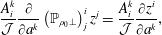 $$\begin{eqnarray}\frac{A_{i}^{k}}{{\mathcal{J}}}\frac{\unicode[STIX]{x2202}}{\unicode[STIX]{x2202}a^{k}}\left(\mathbb{P}_{\unicode[STIX]{x1D70C}_{0}\bot }\right)_{j}^{i}z^{j}=\frac{A_{i}^{k}}{{\mathcal{J}}}\frac{\unicode[STIX]{x2202}z^{i}}{\unicode[STIX]{x2202}a^{k}},\end{eqnarray}$$
 and (4.42). Also, upon inserting  $\mathbb{P}_{\unicode[STIX]{x1D70C}_{0}\bot }=\unicode[STIX]{x1D644}-\mathbb{P}_{\unicode[STIX]{x1D70C}_{0}}$ in the last line of (4.48), symmetry implies we can drop the $\mathbb{P}_{\unicode[STIX]{x1D70C}_{0}\bot }$. Finally, upon substituting (4.48) into (4.30), we obtain
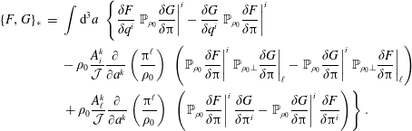 $$\begin{eqnarray}\displaystyle \{F,G\}_{\ast } & = & \displaystyle \int \text{d}^{3}a\,\,\left\{\frac{\unicode[STIX]{x1D6FF}F}{\unicode[STIX]{x1D6FF}q^{i}}\left.\mathbb{P}_{\unicode[STIX]{x1D70C}_{0}}\frac{\unicode[STIX]{x1D6FF}G}{\unicode[STIX]{x1D6FF}\unicode[STIX]{x03C0}}\right|^{i}-\frac{\unicode[STIX]{x1D6FF}G}{\unicode[STIX]{x1D6FF}q^{i}}\left.\mathbb{P}_{\unicode[STIX]{x1D70C}_{0}}\frac{\unicode[STIX]{x1D6FF}F}{\unicode[STIX]{x1D6FF}\unicode[STIX]{x03C0}}\right|^{i}\right.\nonumber\\ \displaystyle & & \displaystyle -\,\unicode[STIX]{x1D70C}_{0}\frac{A_{i}^{k}}{{\mathcal{J}}}\frac{\unicode[STIX]{x2202}}{\unicode[STIX]{x2202}a^{k}}\left(\frac{\unicode[STIX]{x03C0}^{\ell }}{\unicode[STIX]{x1D70C}_{0}}\right)\,\left(\left.\mathbb{P}_{\unicode[STIX]{x1D70C}_{0}}\frac{\unicode[STIX]{x1D6FF}F}{\unicode[STIX]{x1D6FF}\unicode[STIX]{x03C0}}\right|^{i}\left.\mathbb{P}_{\unicode[STIX]{x1D70C}_{0}\bot }\frac{\unicode[STIX]{x1D6FF}G}{\unicode[STIX]{x1D6FF}\unicode[STIX]{x03C0}}\right|_{\ell }-\left.\mathbb{P}_{\unicode[STIX]{x1D70C}_{0}}\frac{\unicode[STIX]{x1D6FF}G}{\unicode[STIX]{x1D6FF}\unicode[STIX]{x03C0}}\right|^{i}\left.\mathbb{P}_{\unicode[STIX]{x1D70C}_{0}\bot }\frac{\unicode[STIX]{x1D6FF}F}{\unicode[STIX]{x1D6FF}\unicode[STIX]{x03C0}}\right|_{\ell }\right)\nonumber\\ \displaystyle & & \displaystyle \left.+\,\unicode[STIX]{x1D70C}_{0}\frac{A_{\ell }^{k}}{{\mathcal{J}}}\frac{\unicode[STIX]{x2202}}{\unicode[STIX]{x2202}a^{k}}\left(\frac{\unicode[STIX]{x03C0}^{\ell }}{\unicode[STIX]{x1D70C}_{0}}\right)\,\left(\left.\mathbb{P}_{\unicode[STIX]{x1D70C}_{0}}\frac{\unicode[STIX]{x1D6FF}F}{\unicode[STIX]{x1D6FF}\unicode[STIX]{x03C0}}\right|^{i}\frac{\unicode[STIX]{x1D6FF}G}{\unicode[STIX]{x1D6FF}\unicode[STIX]{x03C0}^{i}}-\left.\mathbb{P}_{\unicode[STIX]{x1D70C}_{0}}\frac{\unicode[STIX]{x1D6FF}G}{\unicode[STIX]{x1D6FF}\unicode[STIX]{x03C0}}\right|^{i}\frac{\unicode[STIX]{x1D6FF}F}{\unicode[STIX]{x1D6FF}\unicode[STIX]{x03C0}^{i}}\right)\right\}.\end{eqnarray}$$
 Once more inserting  $\mathbb{P}_{\unicode[STIX]{x1D70C}_{0}\bot }=\unicode[STIX]{x1D644}-\mathbb{P}_{\unicode[STIX]{x1D70C}_{0}}$, rearranging and reindexing gives
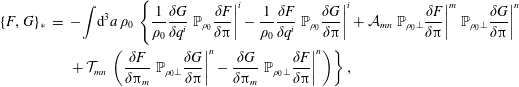 $$\begin{eqnarray}\displaystyle \{F,G\}_{\ast } & = & \displaystyle -\int \text{d}^{3}a\,\unicode[STIX]{x1D70C}_{0}\,\left\{\frac{1}{\unicode[STIX]{x1D70C}_{0}}\frac{\unicode[STIX]{x1D6FF}G}{\unicode[STIX]{x1D6FF}q^{i}}\left.\mathbb{P}_{\unicode[STIX]{x1D70C}_{0}}\frac{\unicode[STIX]{x1D6FF}F}{\unicode[STIX]{x1D6FF}\unicode[STIX]{x03C0}}\right|^{i}-\frac{1}{\unicode[STIX]{x1D70C}_{0}}\frac{\unicode[STIX]{x1D6FF}F}{\unicode[STIX]{x1D6FF}q^{i}}\left.\mathbb{P}_{\unicode[STIX]{x1D70C}_{0}}\frac{\unicode[STIX]{x1D6FF}G}{\unicode[STIX]{x1D6FF}\unicode[STIX]{x03C0}}\right|^{i}+{\mathcal{A}}_{mn}\left.\mathbb{P}_{\unicode[STIX]{x1D70C}_{0}\bot }\frac{\unicode[STIX]{x1D6FF}F}{\unicode[STIX]{x1D6FF}\unicode[STIX]{x03C0}}\right|^{m}\left.\mathbb{P}_{\unicode[STIX]{x1D70C}_{0}\bot }\frac{\unicode[STIX]{x1D6FF}G}{\unicode[STIX]{x1D6FF}\unicode[STIX]{x03C0}}\right|^{n}\right.\nonumber\\ \displaystyle & & \displaystyle \left.+\,{\mathcal{T}}_{mn}\,\left(\frac{\unicode[STIX]{x1D6FF}F}{\unicode[STIX]{x1D6FF}\unicode[STIX]{x03C0}_{m}}\left.\mathbb{P}_{\unicode[STIX]{x1D70C}_{0}\bot }\frac{\unicode[STIX]{x1D6FF}G}{\unicode[STIX]{x1D6FF}\unicode[STIX]{x03C0}}\right|^{n}-\frac{\unicode[STIX]{x1D6FF}G}{\unicode[STIX]{x1D6FF}\unicode[STIX]{x03C0}_{m}}\left.\mathbb{P}_{\unicode[STIX]{x1D70C}_{0}\bot }\frac{\unicode[STIX]{x1D6FF}F}{\unicode[STIX]{x1D6FF}\unicode[STIX]{x03C0}}\right|^{n}\right)\right\},\end{eqnarray}$$
where
 $$\begin{eqnarray}{\mathcal{A}}_{nm}:=\unicode[STIX]{x1D702}_{\ell m}D_{n}^{\ell }-\unicode[STIX]{x1D702}_{\ell n}D_{m}^{\ell }\quad \text{and}\quad {\mathcal{T}}_{mn}:=\unicode[STIX]{x1D702}_{\ell n}D_{m}^{\ell }+\unicode[STIX]{x1D702}_{mn}D^{2},\end{eqnarray}$$
with
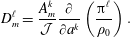 $$\begin{eqnarray}D_{m}^{\ell }=\frac{A_{m}^{k}}{{\mathcal{J}}}\frac{\unicode[STIX]{x2202}}{\unicode[STIX]{x2202}a^{k}}\left(\frac{\unicode[STIX]{x03C0}^{\ell }}{\unicode[STIX]{x1D70C}_{0}}\right).\end{eqnarray}$$
 Note the trace  $D_{\ell }^{\ell }=D^{2}$, which we will eventually set to zero. Equation (4.52) gives the Dirac bracket for the incompressibility holonomic constraint. This bracket with the Hamiltonian
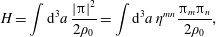 $$\begin{eqnarray}H=\int \text{d}^{3}a\,\frac{|\unicode[STIX]{x03C0}|^{2}}{2\unicode[STIX]{x1D70C}_{0}}=\int \text{d}^{3}a\,\unicode[STIX]{x1D702}^{mn}\frac{\unicode[STIX]{x03C0}_{m}\unicode[STIX]{x03C0}_{n}}{2\unicode[STIX]{x1D70C}_{0}},\end{eqnarray}$$
 produces dynamics that fixes  ${\mathcal{J}}$ and thus enforces incompressibility provided the constraint $D^{2}=0$ is used as an initial condition. For MHD we add to $H$ the following:
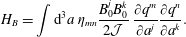 $$\begin{eqnarray}H_{B}=\int \text{d}^{3}a\,\unicode[STIX]{x1D702}_{mn}\frac{B_{0}^{j}B_{0}^{k}}{2{\mathcal{J}}}\,\frac{\unicode[STIX]{x2202}q^{m}}{\unicode[STIX]{x2202}a^{j}}\frac{\unicode[STIX]{x2202}q^{n}}{\unicode[STIX]{x2202}a^{k}}.\end{eqnarray}$$
We note, any Hamiltonian that is consistent with (4.8) can be used to define a constrained flow.
Proceeding to the equations of motion, we first calculate  $\dot{q}^{i}$,
 $$\begin{eqnarray}\displaystyle \dot{q}^{i} & = & \displaystyle \{q^{i},H\}_{\ast }=\left(\mathbb{P}_{\unicode[STIX]{x1D70C}_{0}}\right)_{j}^{i}\frac{\unicode[STIX]{x1D6FF}H}{\unicode[STIX]{x1D6FF}\unicode[STIX]{x03C0}_{j}}=\frac{\unicode[STIX]{x1D6FF}H}{\unicode[STIX]{x1D6FF}\unicode[STIX]{x03C0}_{i}}-\frac{\unicode[STIX]{x1D702}^{i\ell }}{\unicode[STIX]{x1D70C}_{0}}A_{\ell }^{u}\frac{\unicode[STIX]{x2202}}{\unicode[STIX]{x2202}a^{u}}\left[\frac{\unicode[STIX]{x1D6E5}_{\unicode[STIX]{x1D70C}_{0}}^{-1}}{{\mathcal{J}}}\left(\frac{A_{j}^{h}}{{\mathcal{J}}}\frac{\unicode[STIX]{x2202}}{\unicode[STIX]{x2202}a^{h}}\frac{\unicode[STIX]{x1D6FF}H}{\unicode[STIX]{x1D6FF}\unicode[STIX]{x03C0}_{j}}\right)\right]\nonumber\\ \displaystyle & = & \displaystyle \frac{\unicode[STIX]{x03C0}^{i}}{\unicode[STIX]{x1D70C}_{0}}-\frac{\unicode[STIX]{x1D702}^{i\ell }}{\unicode[STIX]{x1D70C}_{0}}A_{\ell }^{u}\frac{\unicode[STIX]{x2202}}{\unicode[STIX]{x2202}a^{u}}\left[\frac{\unicode[STIX]{x1D6E5}_{\unicode[STIX]{x1D70C}_{0}}^{-1}}{{\mathcal{J}}}\left(\frac{A_{j}^{h}}{{\mathcal{J}}}\frac{\unicode[STIX]{x2202}}{\unicode[STIX]{x2202}a^{h}}\frac{\unicode[STIX]{x03C0}^{j}}{\unicode[STIX]{x1D70C}_{0}}\right)\right].\end{eqnarray}$$
 The equation for  $\dot{\unicode[STIX]{x03C0}}_{i}$ is more involved. Using the adjoint property of (4.41), which is valid for both $\mathbb{P}_{\unicode[STIX]{x1D70C}_{0}\bot }$ and $\mathbb{P}_{\unicode[STIX]{x1D70C}_{0}}$, we obtain
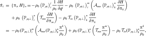 $$\begin{eqnarray}\displaystyle \hspace{-24.0pt}\dot{\unicode[STIX]{x03C0}_{i}} & = & \displaystyle \{\unicode[STIX]{x03C0}_{i},H\}_{\ast }=-\unicode[STIX]{x1D70C}_{0}\left(\mathbb{P}_{\unicode[STIX]{x1D70C}_{0}}\right)_{i}^{j}\frac{1}{\unicode[STIX]{x1D70C}_{0}}\frac{\unicode[STIX]{x1D6FF}H}{\unicode[STIX]{x1D6FF}q^{j}}-\unicode[STIX]{x1D70C}_{0}\,\left(\mathbb{P}_{\unicode[STIX]{x1D70C}_{0}\bot }\right)_{i}^{m}\left({\mathcal{A}}_{mn}\left(\mathbb{P}_{\unicode[STIX]{x1D70C}_{0}\bot }\right)_{k}^{n}\frac{\unicode[STIX]{x1D6FF}H}{\unicode[STIX]{x1D6FF}\unicode[STIX]{x03C0}_{k}}\right)\nonumber\\ \displaystyle \hspace{-24.0pt} & & \displaystyle +\,\unicode[STIX]{x1D70C}_{0}\,\left(\mathbb{P}_{\unicode[STIX]{x1D70C}_{0}\bot }\right)_{i}^{n}\left({\mathcal{T}}_{mn}\frac{\unicode[STIX]{x1D6FF}H}{\unicode[STIX]{x1D6FF}\unicode[STIX]{x03C0}_{m}}\right)-\unicode[STIX]{x1D70C}_{0}\,{\mathcal{T}}_{in}\left(\mathbb{P}_{\unicode[STIX]{x1D70C}_{0}\bot }\right)_{k}^{n}\frac{\unicode[STIX]{x1D6FF}H}{\unicode[STIX]{x1D6FF}\unicode[STIX]{x03C0}_{k}}\nonumber\\ \displaystyle \hspace{-24.0pt} & = & \displaystyle -\unicode[STIX]{x1D70C}_{0}\,(\mathbb{P}_{\unicode[STIX]{x1D70C}_{0}\bot })_{i}^{m}\left({\mathcal{A}}_{mn}(\mathbb{P}_{\unicode[STIX]{x1D70C}_{0}\bot })_{k}^{n}\frac{\unicode[STIX]{x03C0}^{k}}{\unicode[STIX]{x1D70C}_{0}}\right)+\unicode[STIX]{x1D70C}_{0}\,(\mathbb{P}_{\unicode[STIX]{x1D70C}_{0}\bot })_{i}^{n}\left({\mathcal{T}}_{mn}\frac{\unicode[STIX]{x03C0}^{m}}{\unicode[STIX]{x1D70C}_{0}}\right)-\unicode[STIX]{x1D70C}_{0}\,{\mathcal{T}}_{in}(\mathbb{P}_{\unicode[STIX]{x1D70C}_{0}\bot })_{k}^{n}\frac{\unicode[STIX]{x03C0}^{k}}{\unicode[STIX]{x1D70C}_{0}},\nonumber\\ \displaystyle & & \displaystyle\end{eqnarray}$$
 which upon substitution of the definitions of  $\mathbb{P}_{\unicode[STIX]{x1D70C}_{0}}$, ${\mathcal{A}}_{mn}$ and ${\mathcal{T}}_{mn}$ of (4.39) and (4.53) yields a complicated nonlinear equation.
Equations (4.57) and (4.58) are infinite-dimensional versions of the finite-dimensional systems of (2.33) and (2.34) considered in § 2.3.1. There, equations (2.33) and (2.34) were reduced to (2.37) and (2.38) upon enforcing the holomomic constraint by requiring that initially  $D^{2}=0$. Similarly we can enforce the vanishing of $D^{2}$ of (4.8), which is compatible with the Hamiltonian (4.55). Instead of addressing this evaluation now, we find the meaning of various terms is much more transparent when written in terms of Eulerian variables, which we do in § 4.3. We then return to these Lagrangian equations in § 4.4 and make comparisons. Nevertheless, the solution of equations (4.57) and (4.58), $\boldsymbol{q}(\boldsymbol{a},t)$, with the initial conditions $D^{1}=-\ln \unicode[STIX]{x1D70C}_{0}$ and $D^{2}=0$, is a volume preserving transformation at any time $t$.
$t$.
4.3 Eulerian–Dirac constraint theory
Because we chose the form of constraints  $D^{1,2}$ of (4.7) and (4.8) to be Eulerianizable, it follows that we can transform easily the results of § 4.2.1 into Eulerian form. This we do in § 4.3.1. Alternatively, we can proceed as in Nguyen & Turski (Reference Nguyen and Turski1999, Reference Nguyen and Turski2001), Tassi et al. (Reference Tassi, Chandre and Morrison2009), Chandre et al. (Reference Chandre, de Guillebon, Back, Tassi and Morrison2013) and Morrison et al. (Reference Morrison, Lebovitz and Biello2009), starting from the Eulerian noncanonical theory of § 3.3 and directly construct a Dirac bracket with Eulerian constraints. This is a valid procedure because Dirac’s construction works for noncanonical Poisson brackets, as shown, e.g. in Morrison et al. (Reference Morrison, Lebovitz and Biello2009), but it does not readily allow for advected density. This direct method with uniform density is reviewed in § 4.3.2, where it is contrasted with the results of § 4.3.1.
4.3.1 Lagrangian–Dirac constraint theory in the Eulerian picture
In a manner similar to that used to obtain (3.26) and (3.27), we find the functional derivatives transform as
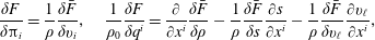 $$\begin{eqnarray}\frac{\unicode[STIX]{x1D6FF}F}{\unicode[STIX]{x1D6FF}\unicode[STIX]{x03C0}_{i}}=\frac{1}{\unicode[STIX]{x1D70C}}\frac{\unicode[STIX]{x1D6FF}\bar{F}}{\unicode[STIX]{x1D6FF}v_{i}},\quad \frac{1}{\unicode[STIX]{x1D70C}_{0}}\frac{\unicode[STIX]{x1D6FF}F}{\unicode[STIX]{x1D6FF}q^{i}}=\frac{\unicode[STIX]{x2202}}{\unicode[STIX]{x2202}x^{i}}\frac{\unicode[STIX]{x1D6FF}\bar{F}}{\unicode[STIX]{x1D6FF}\unicode[STIX]{x1D70C}}-\frac{1}{\unicode[STIX]{x1D70C}}\frac{\unicode[STIX]{x1D6FF}\bar{F}}{\unicode[STIX]{x1D6FF}s}\frac{\unicode[STIX]{x2202}s}{\unicode[STIX]{x2202}x^{i}}-\frac{1}{\unicode[STIX]{x1D70C}}\frac{\unicode[STIX]{x1D6FF}\bar{F}}{\unicode[STIX]{x1D6FF}v_{\ell }}\frac{\unicode[STIX]{x2202}v_{\ell }}{\unicode[STIX]{x2202}x^{i}},\end{eqnarray}$$
 where the expressions on the left of each equality are clearly Lagrangian variable quantities, while on the right they are Eulerian quantities represented in terms of Lagrangian variables. Substituting these expressions into (2.78) and dropping the bar on  $F$ and $G$ gives the following bracket in terms of the Eulerian variables:
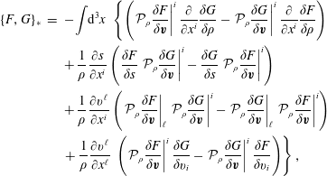 $$\begin{eqnarray}\displaystyle \{F,G\}_{\ast } & = & \displaystyle -\int \text{d}^{3}x\,\,\left\{\left(\left.{\mathcal{P}}_{\unicode[STIX]{x1D70C}}\frac{\unicode[STIX]{x1D6FF}F}{\unicode[STIX]{x1D6FF}\boldsymbol{v}}\right|^{i}\frac{\unicode[STIX]{x2202}}{\unicode[STIX]{x2202}x^{i}}\frac{\unicode[STIX]{x1D6FF}G}{\unicode[STIX]{x1D6FF}\unicode[STIX]{x1D70C}}-\left.{\mathcal{P}}_{\unicode[STIX]{x1D70C}}\frac{\unicode[STIX]{x1D6FF}G}{\unicode[STIX]{x1D6FF}\boldsymbol{v}}\right|^{i}\frac{\unicode[STIX]{x2202}}{\unicode[STIX]{x2202}x^{i}}\frac{\unicode[STIX]{x1D6FF}F}{\unicode[STIX]{x1D6FF}\unicode[STIX]{x1D70C}}\right)\right.\nonumber\\ \displaystyle & & \displaystyle +\,\frac{1}{\unicode[STIX]{x1D70C}}\frac{\unicode[STIX]{x2202}s}{\unicode[STIX]{x2202}x^{i}}\left(\frac{\unicode[STIX]{x1D6FF}F}{\unicode[STIX]{x1D6FF}s}\left.{\mathcal{P}}_{\unicode[STIX]{x1D70C}}\frac{\unicode[STIX]{x1D6FF}G}{\unicode[STIX]{x1D6FF}\boldsymbol{v}}\right|^{i}-\frac{\unicode[STIX]{x1D6FF}G}{\unicode[STIX]{x1D6FF}s}\left.{\mathcal{P}}_{\unicode[STIX]{x1D70C}}\frac{\unicode[STIX]{x1D6FF}F}{\unicode[STIX]{x1D6FF}\boldsymbol{v}}\right|^{i}\right)\nonumber\\ \displaystyle & & \displaystyle +\,\frac{1}{\unicode[STIX]{x1D70C}}\frac{\unicode[STIX]{x2202}v^{\ell }}{\unicode[STIX]{x2202}x^{i}}\left(\left.{\mathcal{P}}_{\unicode[STIX]{x1D70C}}\frac{\unicode[STIX]{x1D6FF}F}{\unicode[STIX]{x1D6FF}\boldsymbol{v}}\right|_{\ell }\left.{\mathcal{P}}_{\unicode[STIX]{x1D70C}}\frac{\unicode[STIX]{x1D6FF}G}{\unicode[STIX]{x1D6FF}\boldsymbol{v}}\right|^{i}-\left.{\mathcal{P}}_{\unicode[STIX]{x1D70C}}\frac{\unicode[STIX]{x1D6FF}G}{\unicode[STIX]{x1D6FF}\boldsymbol{v}}\right|_{\ell }\left.{\mathcal{P}}_{\unicode[STIX]{x1D70C}}\frac{\unicode[STIX]{x1D6FF}F}{\unicode[STIX]{x1D6FF}\boldsymbol{v}}\right|^{i}\right)\nonumber\\ \displaystyle & & \displaystyle \left.+\,\frac{1}{\unicode[STIX]{x1D70C}}\frac{\unicode[STIX]{x2202}v^{\ell }}{\unicode[STIX]{x2202}x^{\ell }}\,\left(\left.{\mathcal{P}}_{\unicode[STIX]{x1D70C}}\frac{\unicode[STIX]{x1D6FF}F}{\unicode[STIX]{x1D6FF}\boldsymbol{v}}\right|^{i}\frac{\unicode[STIX]{x1D6FF}G}{\unicode[STIX]{x1D6FF}v_{i}}-\left.{\mathcal{P}}_{\unicode[STIX]{x1D70C}}\frac{\unicode[STIX]{x1D6FF}G}{\unicode[STIX]{x1D6FF}\boldsymbol{v}}\right|^{i}\frac{\unicode[STIX]{x1D6FF}F}{\unicode[STIX]{x1D6FF}v_{i}}\right)\right\},\end{eqnarray}$$
where we used the relations (3.19) and (3.35) and we introduced the Eulerian projection operator
 $$\begin{eqnarray}\left.{\mathcal{P}}_{\unicode[STIX]{x1D70C}}\frac{\unicode[STIX]{x1D6FF}F}{\unicode[STIX]{x1D6FF}\boldsymbol{v}}\right|^{i}=({\mathcal{P}}_{\unicode[STIX]{x1D70C}})_{j}^{i}\frac{\unicode[STIX]{x1D6FF}F}{\unicode[STIX]{x1D6FF}v_{j}}=\left.\unicode[STIX]{x1D70C}\mathbb{P}_{\unicode[STIX]{x1D70C}_{0}}\frac{\unicode[STIX]{x1D6FF}F}{\unicode[STIX]{x1D6FF}\unicode[STIX]{x03C0}}\right|^{i}\quad \text{and}\quad \left.{\mathcal{P}}_{\unicode[STIX]{x1D70C}}\frac{\unicode[STIX]{x1D6FF}F}{\unicode[STIX]{x1D6FF}\boldsymbol{v}}\right|_{i}=\unicode[STIX]{x1D702}_{ij}\left.{\mathcal{P}}_{\unicode[STIX]{x1D70C}}\frac{\unicode[STIX]{x1D6FF}F}{\unicode[STIX]{x1D6FF}\boldsymbol{v}}\right|^{j},\end{eqnarray}$$
with
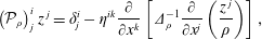 $$\begin{eqnarray}\left({\mathcal{P}}_{\unicode[STIX]{x1D70C}}\right)_{j}^{i}z\,^{j}=\unicode[STIX]{x1D6FF}_{j}^{i}-\unicode[STIX]{x1D702}^{ik}\frac{\unicode[STIX]{x2202}}{\unicode[STIX]{x2202}x^{k}}\left[\unicode[STIX]{x1D6E5}_{\unicode[STIX]{x1D70C}}^{-1}\frac{\unicode[STIX]{x2202}}{\unicode[STIX]{x2202}x^{j}}\left(\frac{z\,^{j}}{\unicode[STIX]{x1D70C}}\right)\right],\end{eqnarray}$$
 which is easily seen to satisfy  $({\mathcal{P}}_{\unicode[STIX]{x1D70C}})_{j}^{i}({\mathcal{P}}_{\unicode[STIX]{x1D70C}})_{k}^{j}=({\mathcal{P}}_{\unicode[STIX]{x1D70C}})_{k}^{i}$. Observe, like its Lagrangian counterpart, ${\mathcal{P}}_{\unicode[STIX]{x1D70C}}$ is formally self-adjoint; however, this time we found it convenient to define the projection in such a way that the self-adjointness is with respect to a different weighted inner product, viz.
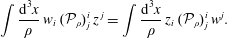 $$\begin{eqnarray}\int \frac{\text{d}^{3}x}{\unicode[STIX]{x1D70C}}\,w_{i}\,({\mathcal{P}}_{\unicode[STIX]{x1D70C}})_{j}^{i}\,z\,^{j}=\int \frac{\text{d}^{3}x}{\unicode[STIX]{x1D70C}}\,z_{i}\,({\mathcal{P}}_{\unicode[STIX]{x1D70C}})_{j}^{i}\,w^{j}.\end{eqnarray}$$
In terms of usual Cartesian vector notation
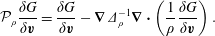 $$\begin{eqnarray}{\mathcal{P}}_{\unicode[STIX]{x1D70C}}\frac{\unicode[STIX]{x1D6FF}G}{\unicode[STIX]{x1D6FF}\boldsymbol{v}}=\frac{\unicode[STIX]{x1D6FF}G}{\unicode[STIX]{x1D6FF}\boldsymbol{v}}-\unicode[STIX]{x1D735}\unicode[STIX]{x1D6E5}_{\unicode[STIX]{x1D70C}}^{-1}\unicode[STIX]{x1D735}\boldsymbol{\cdot }\left(\frac{1}{\unicode[STIX]{x1D70C}}\frac{\unicode[STIX]{x1D6FF}G}{\unicode[STIX]{x1D6FF}\boldsymbol{v}}\right).\end{eqnarray}$$
 Upon writing  ${\mathcal{P}}_{\unicode[STIX]{x1D70C}}=\unicode[STIX]{x1D644}-{\mathcal{P}}_{\unicode[STIX]{x1D70C}\bot }$ and decomposing an arbitrary vector field as
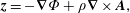 $$\begin{eqnarray}\boldsymbol{z}=-\unicode[STIX]{x1D735}\unicode[STIX]{x1D6F7}+\unicode[STIX]{x1D70C}\unicode[STIX]{x1D735}\times \boldsymbol{A},\end{eqnarray}$$
 this projection operator yields the component  ${\mathcal{P}}_{\unicode[STIX]{x1D70C}}\boldsymbol{z}=\unicode[STIX]{x1D70C}\unicode[STIX]{x1D735}\times \boldsymbol{A}$. Therefore, if $\unicode[STIX]{x1D735}\unicode[STIX]{x1D70C}\times \boldsymbol{A}=0$, then this operator projects into the space of incompressible vector fields. For convenience we introduce the associated projector
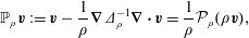 $$\begin{eqnarray}\mathbb{P}_{\unicode[STIX]{x1D70C}}\boldsymbol{v}:=\boldsymbol{v}-\frac{1}{\unicode[STIX]{x1D70C}}\unicode[STIX]{x1D735}\unicode[STIX]{x1D6E5}_{\unicode[STIX]{x1D70C}}^{-1}\unicode[STIX]{x1D735}\boldsymbol{\cdot }\boldsymbol{v}=\frac{1}{\unicode[STIX]{x1D70C}}{\mathcal{P}}_{\unicode[STIX]{x1D70C}}(\unicode[STIX]{x1D70C}\boldsymbol{v}),\end{eqnarray}$$
which has the desirable property
 $$\begin{eqnarray}\unicode[STIX]{x1D735}\boldsymbol{\cdot }(\mathbb{P}_{\unicode[STIX]{x1D70C}}\boldsymbol{v})=0\quad \forall \boldsymbol{v}\quad \text{compared to}\quad \unicode[STIX]{x1D735}\boldsymbol{\cdot }\left(\frac{1}{\unicode[STIX]{x1D70C}}{\mathcal{P}}_{\unicode[STIX]{x1D70C}}\boldsymbol{w}\right)=0\quad \forall \boldsymbol{w}.\end{eqnarray}$$
 Upon writing  $\mathbb{P}_{\unicode[STIX]{x1D70C}}=\unicode[STIX]{x1D644}-\mathbb{P}_{\unicode[STIX]{x1D70C}\bot }$ and decomposing an arbitrary vector field $\boldsymbol{v}$ as
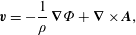 $$\begin{eqnarray}\boldsymbol{v}=-\frac{1}{\unicode[STIX]{x1D70C}}\,\unicode[STIX]{x1D735}\unicode[STIX]{x1D6F7}+\unicode[STIX]{x1D735}\times \boldsymbol{A},\end{eqnarray}$$
 this projection operator yields the component  $\mathbb{P}_{\unicode[STIX]{x1D70C}}\boldsymbol{v}=\unicode[STIX]{x1D735}\times \boldsymbol{A}$, while $\mathbb{P}_{\unicode[STIX]{x1D70C}\bot }\boldsymbol{v}=\unicode[STIX]{x1D735}\unicode[STIX]{x1D6F7}/\unicode[STIX]{x1D70C}$. Note, $\mathbb{P}_{\unicode[STIX]{x1D70C}}$ is the Eulerianization of $\mathbb{P}_{\unicode[STIX]{x1D70C}_{0}}$ and it is not difficult to write (4.69) in terms of this quantity.
Upon adopting this usual vector notation, the bracket (4.60) can also be written as
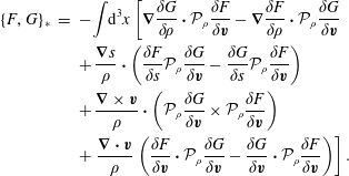 $$\begin{eqnarray}\displaystyle \{F,G\}_{\ast } & = & \displaystyle -\int \text{d}^{3}x\left[\unicode[STIX]{x1D735}\frac{\unicode[STIX]{x1D6FF}G}{\unicode[STIX]{x1D6FF}\unicode[STIX]{x1D70C}}\boldsymbol{\cdot }{\mathcal{P}}_{\unicode[STIX]{x1D70C}}\frac{\unicode[STIX]{x1D6FF}F}{\unicode[STIX]{x1D6FF}\boldsymbol{v}}-\unicode[STIX]{x1D735}\frac{\unicode[STIX]{x1D6FF}F}{\unicode[STIX]{x1D6FF}\unicode[STIX]{x1D70C}}\boldsymbol{\cdot }{\mathcal{P}}_{\unicode[STIX]{x1D70C}}\frac{\unicode[STIX]{x1D6FF}G}{\unicode[STIX]{x1D6FF}\boldsymbol{v}}\right.\nonumber\\ \displaystyle & & \displaystyle +\,\frac{\unicode[STIX]{x1D735}s}{\unicode[STIX]{x1D70C}}\boldsymbol{\cdot }\left(\frac{\unicode[STIX]{x1D6FF}F}{\unicode[STIX]{x1D6FF}s}{\mathcal{P}}_{\unicode[STIX]{x1D70C}}\frac{\unicode[STIX]{x1D6FF}G}{\unicode[STIX]{x1D6FF}\boldsymbol{v}}-\frac{\unicode[STIX]{x1D6FF}G}{\unicode[STIX]{x1D6FF}s}{\mathcal{P}}_{\unicode[STIX]{x1D70C}}\frac{\unicode[STIX]{x1D6FF}F}{\unicode[STIX]{x1D6FF}\boldsymbol{v}}\right)\nonumber\\ \displaystyle & & \displaystyle +\,\frac{\unicode[STIX]{x1D735}\times \boldsymbol{v}}{\unicode[STIX]{x1D70C}}\boldsymbol{\cdot }\left({\mathcal{P}}_{\unicode[STIX]{x1D70C}}\frac{\unicode[STIX]{x1D6FF}G}{\unicode[STIX]{x1D6FF}\boldsymbol{v}}\times {\mathcal{P}}_{\unicode[STIX]{x1D70C}}\frac{\unicode[STIX]{x1D6FF}F}{\unicode[STIX]{x1D6FF}\boldsymbol{v}}\right)\nonumber\\ \displaystyle & & \displaystyle +\left.\frac{\unicode[STIX]{x1D735}\boldsymbol{\cdot }\boldsymbol{v}}{\unicode[STIX]{x1D70C}}\left(\frac{\unicode[STIX]{x1D6FF}F}{\unicode[STIX]{x1D6FF}\boldsymbol{v}}\boldsymbol{\cdot }{\mathcal{P}}_{\unicode[STIX]{x1D70C}}\frac{\unicode[STIX]{x1D6FF}G}{\unicode[STIX]{x1D6FF}\boldsymbol{v}}-\frac{\unicode[STIX]{x1D6FF}G}{\unicode[STIX]{x1D6FF}\boldsymbol{v}}\boldsymbol{\cdot }{\mathcal{P}}_{\unicode[STIX]{x1D70C}}\frac{\unicode[STIX]{x1D6FF}F}{\unicode[STIX]{x1D6FF}\boldsymbol{v}}\right)\right].\end{eqnarray}$$
For MHD there is a magnetic field contribution to (4.59) and following the steps that lead to (4.69) we obtain
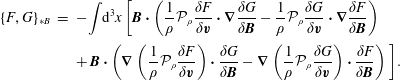 $$\begin{eqnarray}\displaystyle \{F,G\}_{\ast B} & = & \displaystyle -\int \text{d}^{3}x\,\Bigg[\boldsymbol{B}\boldsymbol{\cdot }\left(\frac{1}{\unicode[STIX]{x1D70C}}{\mathcal{P}}_{\unicode[STIX]{x1D70C}}\frac{\unicode[STIX]{x1D6FF}F}{\unicode[STIX]{x1D6FF}\boldsymbol{v}}\boldsymbol{\cdot }\unicode[STIX]{x1D735}\frac{\unicode[STIX]{x1D6FF}G}{\unicode[STIX]{x1D6FF}\boldsymbol{B}}-\frac{1}{\unicode[STIX]{x1D70C}}{\mathcal{P}}_{\unicode[STIX]{x1D70C}}\frac{\unicode[STIX]{x1D6FF}G}{\unicode[STIX]{x1D6FF}\boldsymbol{v}}\boldsymbol{\cdot }\unicode[STIX]{x1D735}\frac{\unicode[STIX]{x1D6FF}F}{\unicode[STIX]{x1D6FF}\boldsymbol{B}}\right)\nonumber\\ \displaystyle & & \displaystyle +\,\boldsymbol{B}\boldsymbol{\cdot }\left(\unicode[STIX]{x1D735}\left(\frac{1}{\unicode[STIX]{x1D70C}}{\mathcal{P}}_{\unicode[STIX]{x1D70C}}\frac{\unicode[STIX]{x1D6FF}F}{\unicode[STIX]{x1D6FF}\boldsymbol{v}}\right)\boldsymbol{\cdot }\frac{\unicode[STIX]{x1D6FF}G}{\unicode[STIX]{x1D6FF}\boldsymbol{B}}-\unicode[STIX]{x1D735}\left(\frac{1}{\unicode[STIX]{x1D70C}}{\mathcal{P}}_{\unicode[STIX]{x1D70C}}\frac{\unicode[STIX]{x1D6FF}G}{\unicode[STIX]{x1D6FF}\boldsymbol{v}}\right)\boldsymbol{\cdot }\frac{\unicode[STIX]{x1D6FF}F}{\unicode[STIX]{x1D6FF}\boldsymbol{B}}\right)\Bigg].\end{eqnarray}$$
 With the exception of the last term of (4.69) proportional to  $\unicode[STIX]{x1D735}\boldsymbol{\cdot }\boldsymbol{v}$ and the presence of the Eulerian projection operator ${\mathcal{P}}_{\unicode[STIX]{x1D70C}}$, equation (4.69) added to (4.70) is identical to the noncanonical Poisson bracket for the ideal fluid and MHD as given in Morrison & Greene (Reference Morrison and Greene1980). By construction, we know that (4.69) satisfies the Jacobi identity – this follows because it was obtained by Eulerianizing the canonical Dirac bracket in terms of Lagrangian variables. Guessing the bracket and proving Jacobi for (4.69) directly would be a difficult chore, giving credence to the path we have followed in obtaining it.
To summarize, the bracket of (4.69) together with the Hamiltonian
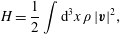 $$\begin{eqnarray}H=\frac{1}{2}\int \text{d}^{3}x\,\unicode[STIX]{x1D70C}\,|\boldsymbol{v}|^{2},\end{eqnarray}$$
 the Eulerian counterpart of (4.55), generates dynamics that can preserve the constraint  $\unicode[STIX]{x1D735}\boldsymbol{\cdot }\boldsymbol{v}=0$. If we add $H_{B}=\int \text{d}^{3}x\,|\boldsymbol{B}|^{2}/2$ to (4.71) and add (4.70) to (4.69), then we obtain incompressible MHD. The fluid case is the Eulerian counterpart of the volume preserving geodesic flow, described originally by Lagrange in Lagrange variables. Upon performing a series of straightforward manipulations, we obtain the following equations of motion for the flow:
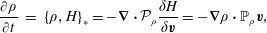 $$\begin{eqnarray}\displaystyle \frac{\unicode[STIX]{x2202}\unicode[STIX]{x1D70C}}{\unicode[STIX]{x2202}t} & = & \displaystyle \left\{\unicode[STIX]{x1D70C},H\right\}_{\ast }=-\unicode[STIX]{x1D735}\boldsymbol{\cdot }{\mathcal{P}}_{\unicode[STIX]{x1D70C}}\frac{\unicode[STIX]{x1D6FF}H}{\unicode[STIX]{x1D6FF}\boldsymbol{v}}=-\unicode[STIX]{x1D735}\unicode[STIX]{x1D70C}\boldsymbol{\cdot }\mathbb{P}_{\unicode[STIX]{x1D70C}}\boldsymbol{v},\end{eqnarray}$$
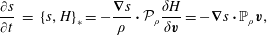 $$\begin{eqnarray}\displaystyle \frac{\unicode[STIX]{x2202}s}{\unicode[STIX]{x2202}t} & = & \displaystyle \left\{s,H\right\}_{\ast }=-\frac{\unicode[STIX]{x1D735}s}{\unicode[STIX]{x1D70C}}\boldsymbol{\cdot }{\mathcal{P}}_{\unicode[STIX]{x1D70C}}\frac{\unicode[STIX]{x1D6FF}H}{\unicode[STIX]{x1D6FF}\boldsymbol{v}}=-\unicode[STIX]{x1D735}s\boldsymbol{\cdot }\mathbb{P}_{\unicode[STIX]{x1D70C}}\boldsymbol{v},\end{eqnarray}$$
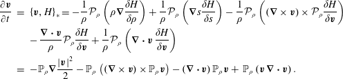 $$\begin{eqnarray}\displaystyle \frac{\unicode[STIX]{x2202}\boldsymbol{v}}{\unicode[STIX]{x2202}t} & = & \displaystyle \left\{\boldsymbol{v},H\right\}_{\ast }=-\frac{1}{\unicode[STIX]{x1D70C}}{\mathcal{P}}_{\unicode[STIX]{x1D70C}}\left(\unicode[STIX]{x1D70C}\unicode[STIX]{x1D735}\frac{\unicode[STIX]{x1D6FF}H}{\unicode[STIX]{x1D6FF}\unicode[STIX]{x1D70C}}\right)+\frac{1}{\unicode[STIX]{x1D70C}}{\mathcal{P}}_{\unicode[STIX]{x1D70C}}\left(\unicode[STIX]{x1D735}s\frac{\unicode[STIX]{x1D6FF}H}{\unicode[STIX]{x1D6FF}s}\right)-\frac{1}{\unicode[STIX]{x1D70C}}{\mathcal{P}}_{\unicode[STIX]{x1D70C}}\left((\unicode[STIX]{x1D735}\times \boldsymbol{v})\times {\mathcal{P}}_{\unicode[STIX]{x1D70C}}\frac{\unicode[STIX]{x1D6FF}H}{\unicode[STIX]{x1D6FF}\boldsymbol{v}}\right)\nonumber\\ \displaystyle & & \displaystyle -\,\frac{\unicode[STIX]{x1D735}\boldsymbol{\cdot }\boldsymbol{v}}{\unicode[STIX]{x1D70C}}{\mathcal{P}}_{\unicode[STIX]{x1D70C}}\frac{\unicode[STIX]{x1D6FF}H}{\unicode[STIX]{x1D6FF}\boldsymbol{v}}+\frac{1}{\unicode[STIX]{x1D70C}}{\mathcal{P}}_{\unicode[STIX]{x1D70C}}\left(\unicode[STIX]{x1D735}\boldsymbol{\cdot }\boldsymbol{v}\,\frac{\unicode[STIX]{x1D6FF}H}{\unicode[STIX]{x1D6FF}\boldsymbol{v}}\right)\nonumber\\ \displaystyle & = & \displaystyle -\mathbb{P}_{\unicode[STIX]{x1D70C}}\unicode[STIX]{x1D735}\frac{|\boldsymbol{v}|^{2}}{2}-\mathbb{P}_{\unicode[STIX]{x1D70C}}\left((\unicode[STIX]{x1D735}\times \boldsymbol{v})\times \mathbb{P}_{\unicode[STIX]{x1D70C}}\boldsymbol{v}\right)-(\unicode[STIX]{x1D735}\boldsymbol{\cdot }\boldsymbol{v})\,\mathbb{P}_{\unicode[STIX]{x1D70C}}\boldsymbol{v}+\,\mathbb{P}_{\unicode[STIX]{x1D70C}}\left(\boldsymbol{v}\,\unicode[STIX]{x1D735}\boldsymbol{\cdot }\boldsymbol{v}\right).\end{eqnarray}$$
 If we include  $H_{B}$ we obtain additional terms to (4.74) generated by (4.70) for the projected $\boldsymbol{J}\times \boldsymbol{B}$ force. Observe, equation (4.74) is not yet evaluated on the constraint $D^{2}=0$, which in Eulerian variables is $\unicode[STIX]{x1D735}\boldsymbol{\cdot }\boldsymbol{v}=0$. As noted at the end of § 4.2, we turn to this task in § 4.4.
4.3.2 Eulerian–Dirac constraint theory direct with uniform density
For completeness we recall the simpler case where the Eulerian density  $\unicode[STIX]{x1D70C}$ is uniformly constant, which without loss of generality can be scaled to unity. This case was considered in Nguyen & Turski (Reference Nguyen and Turski1999, Reference Nguyen and Turski2001) and Chandre et al. (Reference Chandre, Morrison and Tassi2012, Reference Chandre, de Guillebon, Back, Tassi and Morrison2013) (although a trick of using entropy as density was employed in Chandre et al. (Reference Chandre, de Guillebon, Back, Tassi and Morrison2013) to treat density advection). In these works the Dirac constraints were chosen to be the pointwise Eulerian quantities
 $$\begin{eqnarray}{\mathcal{D}}^{1}=\unicode[STIX]{x1D70C}\quad \text{and}\quad {\mathcal{D}}^{2}=\unicode[STIX]{x1D735}\boldsymbol{\cdot }\boldsymbol{v},\end{eqnarray}$$
and the Dirac procedure was effected on the purely Eulerian level. This led to the projector
 $$\begin{eqnarray}\mathbb{P}:=\mathbb{P}_{\unicode[STIX]{x1D70C}=1}=1-\unicode[STIX]{x1D735}\unicode[STIX]{x1D6E5}^{-1}\unicode[STIX]{x1D735}\,\boldsymbol{\cdot },\end{eqnarray}$$
 where  $\unicode[STIX]{x1D6E5}=\unicode[STIX]{x1D6E5}_{\unicode[STIX]{x1D70C}=1}$, and the following Dirac bracket:
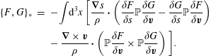 $$\begin{eqnarray}\displaystyle \{F,G\}_{\ast } & = & \displaystyle -\int \text{d}^{3}x\,\Bigg[\frac{\unicode[STIX]{x1D735}s}{\unicode[STIX]{x1D70C}}\boldsymbol{\cdot }\left(\frac{\unicode[STIX]{x1D6FF}F}{\unicode[STIX]{x1D6FF}s}\mathbb{P}\frac{\unicode[STIX]{x1D6FF}G}{\unicode[STIX]{x1D6FF}\boldsymbol{v}}-\frac{\unicode[STIX]{x1D6FF}G}{\unicode[STIX]{x1D6FF}s}\mathbb{P}\frac{\unicode[STIX]{x1D6FF}F}{\unicode[STIX]{x1D6FF}\boldsymbol{v}}\right)\nonumber\\ \displaystyle & & \displaystyle -\,\frac{\unicode[STIX]{x1D735}\times \boldsymbol{v}}{\unicode[STIX]{x1D70C}}\boldsymbol{\cdot }\left(\mathbb{P}\frac{\unicode[STIX]{x1D6FF}F}{\unicode[STIX]{x1D6FF}\boldsymbol{v}}\times \mathbb{P}\frac{\unicode[STIX]{x1D6FF}G}{\unicode[STIX]{x1D6FF}\boldsymbol{v}}\right)\Bigg].\end{eqnarray}$$
Incompressible MHD with constant density is generated by adding the following to (4.77):
 $$\begin{eqnarray}\displaystyle \{F,G\}_{\ast B} & = & \displaystyle -\int \text{d}^{3}x\,\left[\frac{\boldsymbol{B}}{\unicode[STIX]{x1D70C}}\boldsymbol{\cdot }\left(\mathbb{P}\frac{\unicode[STIX]{x1D6FF}F}{\unicode[STIX]{x1D6FF}\boldsymbol{v}}\boldsymbol{\cdot }\unicode[STIX]{x1D735}\frac{\unicode[STIX]{x1D6FF}G}{\unicode[STIX]{x1D6FF}\boldsymbol{B}}-\mathbb{P}\frac{\unicode[STIX]{x1D6FF}G}{\unicode[STIX]{x1D6FF}\boldsymbol{v}}\boldsymbol{\cdot }\unicode[STIX]{x1D735}\frac{\unicode[STIX]{x1D6FF}F}{\unicode[STIX]{x1D6FF}\boldsymbol{B}}\right)\right.\nonumber\\ \displaystyle & & \displaystyle \left.+\,\boldsymbol{B}\boldsymbol{\cdot }\left(\unicode[STIX]{x1D735}\left(\frac{1}{\unicode[STIX]{x1D70C}}\mathbb{P}\frac{\unicode[STIX]{x1D6FF}F}{\unicode[STIX]{x1D6FF}\boldsymbol{v}}\right)\boldsymbol{\cdot }\frac{\unicode[STIX]{x1D6FF}G}{\unicode[STIX]{x1D6FF}\boldsymbol{B}}-\unicode[STIX]{x1D735}\left(\frac{1}{\unicode[STIX]{x1D70C}}\mathbb{P}\frac{\unicode[STIX]{x1D6FF}G}{\unicode[STIX]{x1D6FF}\boldsymbol{v}}\right)\boldsymbol{\cdot }\frac{\unicode[STIX]{x1D6FF}F}{\unicode[STIX]{x1D6FF}\boldsymbol{B}}\right)\right],\end{eqnarray}$$
 and adding  $|\boldsymbol{B}|^{2}/2$ to the integrand of (4.71).
The bracket of (4.77) differs from that of (4.69) in two ways: the projector  ${\mathcal{P}}_{\unicode[STIX]{x1D70C}}$ is replaced by the simpler projector $\mathbb{P}$ and it is missing the term proportional to $\unicode[STIX]{x1D735}\boldsymbol{\cdot }\boldsymbol{v}$. Given that $\unicode[STIX]{x1D735}\boldsymbol{\cdot }\boldsymbol{v}$ cannot be set to zero until after the equations of motion are obtained, this term gives rise to significant differences between the constant and non-constant density Poisson brackets and incompressible dynamics.
4.4 Comparison of the Eulerian–Dirac and Lagrangian–Dirac constrained theories
Let us now discuss equations (4.72), (4.73) and (4.74). Given that  $\unicode[STIX]{x1D735}\boldsymbol{\cdot }\mathbb{P}_{\unicode[STIX]{x1D70C}}\boldsymbol{v}=0$ (cf. (4.67)) it is clear that the density and entropy are advected by the incompressible velocity field $\mathbb{P}_{\unicode[STIX]{x1D70C}}\boldsymbol{v}$, as expected. However, the meaning of (4.74) remains to be clarified. To this end we take the divergence of (4.74) and again use (4.67) to obtain
 $$\begin{eqnarray}\frac{\unicode[STIX]{x2202}(\unicode[STIX]{x1D735}\boldsymbol{\cdot }\boldsymbol{v})}{\unicode[STIX]{x2202}t}=-\unicode[STIX]{x1D735}\boldsymbol{\cdot }\left(\unicode[STIX]{x1D735}\boldsymbol{\cdot }\boldsymbol{v}\,\mathbb{P}_{\unicode[STIX]{x1D70C}}\boldsymbol{v}\right)=-\left(\mathbb{P}_{\unicode[STIX]{x1D70C}}\boldsymbol{v}\right)\boldsymbol{\cdot }\!\unicode[STIX]{x1D735}\,(\unicode[STIX]{x1D735}\boldsymbol{\cdot }\boldsymbol{v}).\end{eqnarray}$$
 Thus  $\unicode[STIX]{x1D735}\boldsymbol{\cdot }\boldsymbol{v}$ itself is advected by an incompressible velocity field. As with any advection equation, if initially $\unicode[STIX]{x1D735}\boldsymbol{\cdot }\boldsymbol{v}=0$ , it will remain uniformly zero. After setting $\unicode[STIX]{x1D735}\boldsymbol{\cdot }\boldsymbol{v}=0$ in (4.74) it collapses down to
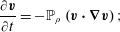 $$\begin{eqnarray}\frac{\unicode[STIX]{x2202}\boldsymbol{v}}{\unicode[STIX]{x2202}t}=-\mathbb{P}_{\unicode[STIX]{x1D70C}}\left(\boldsymbol{v}\boldsymbol{\cdot }\unicode[STIX]{x1D735}\boldsymbol{v}\right);\end{eqnarray}$$
this is the anticipated equation of motion, the momentum equation of (1.1) with the insertion of the pressure given by (1.5).
Given the discussion of Lagrangian versus Eulerian constants of motion of § 3.4, that  $\unicode[STIX]{x1D735}\boldsymbol{\cdot }\boldsymbol{v}$ is advected rather than pointwise conserved is to be expected. Our development began with the constraints $D^{1,2}$ of (4.7) and (4.8) both of which are pointwise conserved by the Dirac procedure, i.e. $\dot{{\mathcal{D}}}_{L}\equiv 0$. This means their corresponding fluxes are identically zero, i.e. in (3.38) we have $\unicode[STIX]{x1D6E4}_{{\mathcal{D}}_{L}}\equiv 0$ for each. Thus the flux component $\bar{\unicode[STIX]{x1D6E4}}_{{\mathcal{D}}_{E}}$ of (3.42) vanishes and the Eulerian flux for both $D^{1}$ and $D^{2}$ have the form $\boldsymbol{v}{\mathcal{D}}_{E}$. Because $D^{1}$ and $D^{2}$ Eulerianize to $-\ln (\unicode[STIX]{x1D70C})$ and $\unicode[STIX]{x1D735}\boldsymbol{\cdot }\boldsymbol{v}$, respectively, we expected equations of the from of (4.79) for both. We will see in § 4.5 that the equation for $D^{1}$ in fact follows also because the constraints are Casimir invariants.
Let us return to (4.58) and compare with the results of § 2.3.1. Because the incompressibility condition is an holonomic constraint and § 2.3.1 concerns holonomic constraints for the uncoupled  $N$-body problem, both results are geodesic flows. In fact, one can think of the fluid case as a continuum version of that of § 2.3.1 with an infinity of holonomic constraints – thus we expect similarities between these results. However, because the incompressibility constraints are pointwise constraints, the comparison is not as straightforward as it would be for global constraints of the fluid.
To make the comparison we first observe that the term  ${\mathcal{A}}_{mn}$ of (4.52) must correspond to the term $\overset{\leftrightarrow }{\mathbb{A}}_{ij}$ of (2.47), since their origin follows an analogous path in the derivation, both are antisymmetric, and both project from both the left and the right. The analogue of (2.49) according to (4.39) is
 $$\begin{eqnarray}\left(\mathbb{P}_{\unicode[STIX]{x1D70C}_{0}\bot }\right)_{j}^{i}\,\frac{\unicode[STIX]{x03C0}^{j}}{\unicode[STIX]{x1D70C}_{0}}=\frac{\unicode[STIX]{x1D702}^{i\ell }}{\unicode[STIX]{x1D70C}_{0}}A_{\ell }^{u}\frac{\unicode[STIX]{x2202}}{\unicode[STIX]{x2202}a^{u}}\left[\frac{\unicode[STIX]{x1D6E5}_{\unicode[STIX]{x1D70C}_{0}}^{-1}}{{\mathcal{J}}}\left(\frac{A_{j}^{h}}{{\mathcal{J}}}\frac{\unicode[STIX]{x2202}}{\unicode[STIX]{x2202}a^{h}}\,\frac{\unicode[STIX]{x03C0}^{j}}{\unicode[STIX]{x1D70C}_{0}}\right)\right]=\frac{\unicode[STIX]{x1D702}^{i\ell }}{\unicode[STIX]{x1D70C}_{0}}A_{\ell }^{u}\frac{\unicode[STIX]{x2202}}{\unicode[STIX]{x2202}a^{u}}\left[\frac{\unicode[STIX]{x1D6E5}_{\unicode[STIX]{x1D70C}_{0}}^{-1}}{{\mathcal{J}}}\left(D^{2}\right)\right]\equiv 0,\end{eqnarray}$$
 when evaluated on  $D^{2}=0$. Unlike (2.49) a sum, which would here be an integral over $\text{d}^{3}a$, does not occur because the constraint $D^{2}$ is a pointwise constraint as opposed to a global constraint. Also, because the constraints are pointwise, the $\overset{\leftrightarrow }{\mathbb{T}}_{ij}$ is analogous to the terms with ${\mathcal{T}}_{mn}$ that also have a factor of the projector $\mathbb{P}_{\unicode[STIX]{x1D70C}_{0}\bot }$, giving the results analogous to (2.50). Just as in § 2.3.1, we obtain $\unicode[STIX]{x03C0}^{i}=\unicode[STIX]{x1D70C}_{0}\dot{q}^{i}$ from (4.57) when evaluated on the constraint $D^{2}=0$ and only a single term involving the ${\mathcal{T}}_{mn}$ contributes to the momentum equation of motion (4.58). We obtain
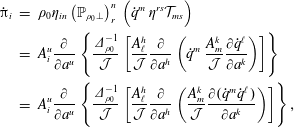 $$\begin{eqnarray}\displaystyle \dot{\unicode[STIX]{x03C0}}_{i} & = & \displaystyle \unicode[STIX]{x1D70C}_{0}\unicode[STIX]{x1D702}_{in}\left(\mathbb{P}_{\unicode[STIX]{x1D70C}_{0}\bot }\right)_{r}^{n}\,\Big(\dot{q}^{m}\,\unicode[STIX]{x1D702}^{rs}{\mathcal{T}}_{ms}\Big)\nonumber\\ \displaystyle & = & \displaystyle A_{i}^{u}\frac{\unicode[STIX]{x2202}}{\unicode[STIX]{x2202}a^{u}}\left\{\frac{\unicode[STIX]{x1D6E5}_{\unicode[STIX]{x1D70C}_{0}}^{-1}}{{\mathcal{J}}}\left[\frac{A_{\ell }^{h}}{{\mathcal{J}}}\frac{\unicode[STIX]{x2202}}{\unicode[STIX]{x2202}a^{h}}\left(\dot{q}^{m}\,\frac{A_{m}^{k}}{{\mathcal{J}}}\frac{\unicode[STIX]{x2202}\dot{q}^{\ell }}{\unicode[STIX]{x2202}a^{k}}\right)\right]\right\}\nonumber\\ \displaystyle & = & \displaystyle A_{i}^{u}\frac{\unicode[STIX]{x2202}}{\unicode[STIX]{x2202}a^{u}}\left\{\frac{\unicode[STIX]{x1D6E5}_{\unicode[STIX]{x1D70C}_{0}}^{-1}}{{\mathcal{J}}}\left[\frac{A_{\ell }^{h}}{{\mathcal{J}}}\frac{\unicode[STIX]{x2202}}{\unicode[STIX]{x2202}a^{h}}\left(\frac{A_{m}^{k}}{{\mathcal{J}}}\frac{\unicode[STIX]{x2202}(\dot{q}^{m}\dot{q}^{\ell })}{\unicode[STIX]{x2202}a^{k}}\right)\right]\right\},\end{eqnarray}$$
where the second equality follows upon substitution of
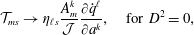 $$\begin{eqnarray}{\mathcal{T}}_{ms}\rightarrow \unicode[STIX]{x1D702}_{\ell s}\frac{A_{m}^{k}}{{\mathcal{J}}}\frac{\unicode[STIX]{x2202}\dot{q}^{\ell }}{\unicode[STIX]{x2202}a^{k}},\quad \text{for }D^{2}=0,\end{eqnarray}$$
 which follows from (4.53), while the third follows again from  $D^{2}=0$ according to (4.8). Thus,
 $$\begin{eqnarray}\displaystyle \ddot{q}^{i} & = & \displaystyle \unicode[STIX]{x1D702}^{i\ell }\frac{A_{\ell }^{u}}{\unicode[STIX]{x1D70C}_{0}}\frac{\unicode[STIX]{x2202}}{\unicode[STIX]{x2202}a^{u}}\left\{\frac{\unicode[STIX]{x1D6E5}_{\unicode[STIX]{x1D70C}_{0}}^{-1}}{{\mathcal{J}}}\left[\frac{A_{j}^{h}}{{\mathcal{J}}}\frac{\unicode[STIX]{x2202}}{\unicode[STIX]{x2202}a^{h}}\left(\frac{A_{k}^{f}}{{\mathcal{J}}}\frac{\unicode[STIX]{x2202}(\dot{q}^{j}\,\dot{q}^{k})}{\unicode[STIX]{x2202}a^{f}}\right)\right]\right\}\nonumber\\ \displaystyle & = & \displaystyle \left(\mathbb{P}_{\unicode[STIX]{x1D70C}_{0}\bot }\right)_{j}^{i}\,\left(\frac{A_{k}^{f}}{{\mathcal{J}}}\frac{\unicode[STIX]{x2202}(\dot{q}^{j}\,\dot{q}^{k})}{\unicode[STIX]{x2202}a^{f}}\right)=:-\,\widehat{\unicode[STIX]{x1D6E4}}_{jk}^{\,i}(\dot{q}^{j},\dot{q}^{k}),\end{eqnarray}$$
 where in (4.84) we have defined  $\widehat{\unicode[STIX]{x1D6E4}}_{jk}^{\,i}(\dot{q}^{j},\dot{q}^{k})$, the normal force operator for geodesic flow, analogous to that of (2.55).
As was the case for the  $\widehat{\unicode[STIX]{x1D6E4}}_{i,jk}$ of (2.56), $\widehat{\unicode[STIX]{x1D6E4}}_{jk}^{\,i}$ possesses symmetry: given arbitrary vector fields $\boldsymbol{V}$ and $\boldsymbol{W}$
 $$\begin{eqnarray}\widehat{\unicode[STIX]{x1D6E4}}_{jk}^{\,i}(V^{j},W^{k}):=-\unicode[STIX]{x1D702}^{i\ell }\frac{A_{\ell }^{u}}{\unicode[STIX]{x1D70C}_{0}}\frac{\unicode[STIX]{x2202}}{\unicode[STIX]{x2202}a^{u}}\left\{\frac{\unicode[STIX]{x1D6E5}_{\unicode[STIX]{x1D70C}_{0}}^{-1}}{{\mathcal{J}}}\left[\frac{A_{j}^{h}}{{\mathcal{J}}}\frac{\unicode[STIX]{x2202}}{\unicode[STIX]{x2202}a^{h}}\left(\frac{A_{k}^{f}}{{\mathcal{J}}}\frac{\unicode[STIX]{x2202}(V^{j}\,W^{k})}{\unicode[STIX]{x2202}a^{f}}\right)\right]\right\}=\widehat{\unicode[STIX]{x1D6E4}}_{jk}^{\,i}(V^{k},W^{j}),\end{eqnarray}$$
where the second equality follows from the commutation relation of (3.9).
Equation (4.84) defines geodesic flow on the group of volume preserving diffeomorphisms, as was the case in § 2.3.1, it does so in terms of the original coordinates, i.e. without specifically transforming to normal coordinates on the constraint surfaces which here are infinite-dimensional.
Now we are in position to close the circle by writing (4.84) in Eulerian form. We will do this for the ideal fluid, but MHD follows similarly. As usual the term  $\ddot{q}^{i}$ becomes the advective derivative $\unicode[STIX]{x2202}\boldsymbol{v}/\unicode[STIX]{x2202}t+\boldsymbol{v}\boldsymbol{\cdot }\unicode[STIX]{x1D735}\boldsymbol{v}$, the projector $\mathbb{P}_{\unicode[STIX]{x1D70C}_{0}\bot }$ becomes $\mathbb{P}_{\unicode[STIX]{x1D70C}\bot }$ (using $\unicode[STIX]{x1D6E5}_{\unicode[STIX]{x1D70C}_{0}}^{-1}={\mathcal{J}}\unicode[STIX]{x1D6E5}_{\unicode[STIX]{x1D70C}}^{-1}$) when Eulerianized, and the $\widehat{\unicode[STIX]{x1D6E4}}_{jk}^{i}$ term becomes $\mathbb{P}_{\unicode[STIX]{x1D70C}\bot }\left(\unicode[STIX]{x1D735}\boldsymbol{\cdot }(\boldsymbol{v}\otimes \boldsymbol{v})\right)$. Thus (4.84) is precisely the Lagrangian form of (4.80), written as follows:
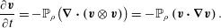 $$\begin{eqnarray}\frac{\unicode[STIX]{x2202}\boldsymbol{v}}{\unicode[STIX]{x2202}t}=-\mathbb{P}_{\unicode[STIX]{x1D70C}}\big(\unicode[STIX]{x1D735}\boldsymbol{\cdot }(\boldsymbol{v}\otimes \boldsymbol{v})\big)=-\mathbb{P}_{\unicode[STIX]{x1D70C}}\left(\boldsymbol{v}\boldsymbol{\cdot }\unicode[STIX]{x1D735}\boldsymbol{v}\right).\end{eqnarray}$$
Similarly, the Lagrangian version of (4.79) follows easily from (4.84). To see this we operate with the counterpart of taking the Eulerian divergence on the first line of (4.82) and make use of (4.50),
 $$\begin{eqnarray}\displaystyle \frac{A_{n}^{h}}{{\mathcal{J}}}\frac{\unicode[STIX]{x2202}}{\unicode[STIX]{x2202}a^{h}}\frac{\dot{\unicode[STIX]{x03C0}}^{n}}{\unicode[STIX]{x1D70C}_{0}} & = & \displaystyle \frac{A_{n}^{h}}{{\mathcal{J}}}\frac{\unicode[STIX]{x2202}}{\unicode[STIX]{x2202}a^{h}}(\mathbb{P}_{\unicode[STIX]{x1D70C}_{0}\bot })_{r}^{n}\,\Big(\dot{q}^{m}\,\unicode[STIX]{x1D702}^{rs}{\mathcal{T}}_{ms}\Big)=\frac{A_{n}^{h}}{{\mathcal{J}}}\frac{\unicode[STIX]{x2202}}{\unicode[STIX]{x2202}a^{h}}\Big(\dot{q}^{m}\,\unicode[STIX]{x1D702}^{ns}{\mathcal{T}}_{ms}\Big)\nonumber\\ \displaystyle & = & \displaystyle \unicode[STIX]{x1D6FF}_{\ell }^{n}\frac{A_{n}^{h}}{{\mathcal{J}}}\frac{\unicode[STIX]{x2202}}{\unicode[STIX]{x2202}a^{h}}\left(\dot{q}^{m}\frac{A_{m}^{k}}{{\mathcal{J}}}\frac{\unicode[STIX]{x2202}\dot{q}^{\ell }}{\unicode[STIX]{x2202}a^{k}}\right),\end{eqnarray}$$
which in Eulerian variables becomes
 $$\begin{eqnarray}\unicode[STIX]{x1D735}\boldsymbol{\cdot }\left(\frac{\unicode[STIX]{x2202}\boldsymbol{v}}{\unicode[STIX]{x2202}t}+\boldsymbol{v}\boldsymbol{\cdot }\unicode[STIX]{x1D735}\boldsymbol{v}\right)=\unicode[STIX]{x1D735}\boldsymbol{\cdot }(\boldsymbol{v}\boldsymbol{\cdot }\unicode[STIX]{x1D735}\boldsymbol{v})\quad \text{or}\quad \unicode[STIX]{x1D735}\boldsymbol{\cdot }\frac{\unicode[STIX]{x2202}\boldsymbol{v}}{\unicode[STIX]{x2202}t}=\frac{\unicode[STIX]{x2202}\,}{\unicode[STIX]{x2202}t}\unicode[STIX]{x1D735}\boldsymbol{\cdot }\boldsymbol{v}=0.\end{eqnarray}$$
In Lagrangian variables we have the trivial conservation laws
 $$\begin{eqnarray}\dot{\unicode[STIX]{x1D70C}_{0}}=0\quad \text{and}\quad \dot{s_{0}}=0,\end{eqnarray}$$
 where the corresponding fluxes are identically zero. However, as is evident from (4.72) and (4.73) we obtain non-trivial conservation laws for  $\unicode[STIX]{x1D70C}$ and $s$ with non-zero fluxes. Thus we see again, consistent with § 3.4, how Lagrangian and Eulerian conservation laws are not equivalent.
For the special case where  $\unicode[STIX]{x1D70C}_{0}={\mathcal{J}}=1$ one could proceed directly from (1.7), write it in terms of the Lagrangian variables, and obtain (4.84). However, without the constraint theory, one would not immediately see it is Hamiltonian and in fact geodesic flow on an infinite-dimensional manifold.
4.5 Incompressible algebra of invariants
In closing this section, we examine the constants of motion for the constrained system. The Poisson bracket together with the set of functionals that commute with the Hamiltonian, i.e. that satisfy  $\{H,I_{a}\}=0$ for $a=1,2,\ldots ,d$, constitute the $d$-dimensional algebra of invariants, a subalgebra of the infinite-dimensional Poisson bracket realization on all functionals. This subalgebra is a Lie algebra realization associated with a symmetry group of the dynamical system, and the Poisson bracket with $\{I_{a},\boldsymbol{\cdot }\,\}$ yields the infinitesimal generators of the symmetries, i.e. the differential operator realization of the algebra. This was shown for compressible MHD in Morrison (Reference Morrison1982), where the associated Lie algebra realization of the 10 parameter Galilean group on functionals was described. This algebra is homomorphic to usual representations of the Galilean group, with the Casimir invariants being in the centre of the algebra composed of elements that have vanishing Poisson bracket with all other elements.
A natural question to ask is what happens to this algebra when incompressibility is enforced by our Dirac constraint procedure. Obviously the Hamiltonian is in the subalgebra and  $\{H,\boldsymbol{\cdot }\,\}_{\ast }$ clearly generates time translation, and this will be true for any Hamiltonian, but here we use Hamiltonian of (4.71).
Inserting the momentum
 $$\begin{eqnarray}\boldsymbol{P}=\int \text{d}^{3}x\,\unicode[STIX]{x1D70C}\boldsymbol{v}\end{eqnarray}$$
into (4.69) with the Hamiltonian (4.71) gives
 $$\begin{eqnarray}\{\boldsymbol{P},H\}_{\ast }=0\end{eqnarray}$$
 without assuming  $\unicode[STIX]{x1D735}\boldsymbol{\cdot }\boldsymbol{v}=0$. To see this, we use (4.64) to obtain
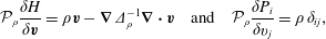 $$\begin{eqnarray}{\mathcal{P}}_{\unicode[STIX]{x1D70C}}\frac{\unicode[STIX]{x1D6FF}H}{\unicode[STIX]{x1D6FF}\boldsymbol{v}}=\unicode[STIX]{x1D70C}\boldsymbol{v}-\unicode[STIX]{x1D735}\unicode[STIX]{x1D6E5}_{\unicode[STIX]{x1D70C}}^{-1}\unicode[STIX]{x1D735}\boldsymbol{\cdot }\boldsymbol{v}\quad \text{and}\quad {\mathcal{P}}_{\unicode[STIX]{x1D70C}}\frac{\unicode[STIX]{x1D6FF}P_{i}}{\unicode[STIX]{x1D6FF}v_{j}}=\unicode[STIX]{x1D70C}\,\unicode[STIX]{x1D6FF}_{ij},\end{eqnarray}$$
which when inserted into (4.69) gives
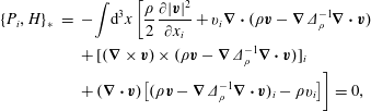 $$\begin{eqnarray}\displaystyle \{P_{i},H\}_{\ast } & = & \displaystyle -\int \text{d}^{3}x\,\bigg[\frac{\unicode[STIX]{x1D70C}}{2}\frac{\unicode[STIX]{x2202}|\boldsymbol{v}|^{2}}{\unicode[STIX]{x2202}x_{i}}+v_{i}\unicode[STIX]{x1D735}\boldsymbol{\cdot }(\unicode[STIX]{x1D70C}\boldsymbol{v}-\unicode[STIX]{x1D735}\unicode[STIX]{x1D6E5}_{\unicode[STIX]{x1D70C}}^{-1}\unicode[STIX]{x1D735}\boldsymbol{\cdot }\boldsymbol{v})\nonumber\\ \displaystyle & & \displaystyle +\,[(\unicode[STIX]{x1D735}\times \boldsymbol{v})\times (\unicode[STIX]{x1D70C}\boldsymbol{v}-\unicode[STIX]{x1D735}\unicode[STIX]{x1D6E5}_{\unicode[STIX]{x1D70C}}^{-1}\unicode[STIX]{x1D735}\boldsymbol{\cdot }\boldsymbol{v})]_{i}\nonumber\\ \displaystyle & & \displaystyle +\,(\unicode[STIX]{x1D735}\boldsymbol{\cdot }\boldsymbol{v})\left[(\unicode[STIX]{x1D70C}\boldsymbol{v}-\unicode[STIX]{x1D735}\unicode[STIX]{x1D6E5}_{\unicode[STIX]{x1D70C}}^{-1}\unicode[STIX]{x1D735}\boldsymbol{\cdot }\boldsymbol{v})_{i}-\unicode[STIX]{x1D70C}v_{i}\right]\bigg]=0,\end{eqnarray}$$
 as expected. The result of (4.93) follows upon using standard vector identities, integration by parts, and the self-adjointness of  $\unicode[STIX]{x1D6E5}_{\unicode[STIX]{x1D70C}}^{-1}$.
The associated generator of space translations that satisfies the constraints is given by the operator  $\{\boldsymbol{P},~\boldsymbol{\cdot }~\}_{\ast }$, which can be shown directly. And, it follows that
 $$\begin{eqnarray}\{P_{i},{P_{j}\}}_{\ast }=0,\quad \forall i,j=1,2,3.\end{eqnarray}$$
 Because the momentum contains no  $s$ dependence the second line of (4.69) vanishes and using ${\mathcal{P}}_{\unicode[STIX]{x1D70C}}\unicode[STIX]{x1D6FF}P_{i}/\unicode[STIX]{x1D6FF}v_{j}=\unicode[STIX]{x1D70C}\,\unicode[STIX]{x1D6FF}_{ij}$ of (4.92) it is clear the last line involving $\unicode[STIX]{x1D735}\boldsymbol{\cdot }\boldsymbol{v}$ of (4.69) also vanishes. The result of (4.94) is obtained because the first and third lines cancel.
Next, consider the angular momentum
 $$\begin{eqnarray}\boldsymbol{L}=\int \text{d}^{3}x\,\unicode[STIX]{x1D70C}\,\boldsymbol{x}\times \boldsymbol{v}.\end{eqnarray}$$
We will show
 $$\begin{eqnarray}\{L_{i},H\}_{\ast }=0.\end{eqnarray}$$
 Using  ${\mathcal{P}}_{\unicode[STIX]{x1D70C}}\unicode[STIX]{x1D6FF}L_{i}/\unicode[STIX]{x1D6FF}\boldsymbol{v}=\unicode[STIX]{x1D6FF}L_{i}/\unicode[STIX]{x1D6FF}\boldsymbol{v}$, which follows from (4.64) with $\unicode[STIX]{x2202}(\unicode[STIX]{x1D716}_{ik\ell }x_{\ell })/\unicode[STIX]{x2202}x^{\ell }=0$, the fact that $\{L_{i},H\}=0$ for the compressible fluid, and ${\mathcal{P}}_{\unicode[STIX]{x1D70C}}=\unicode[STIX]{x1D644}-{\mathcal{P}}_{\unicode[STIX]{x1D70C}\bot }$, we obtain
 $$\begin{eqnarray}\displaystyle \{L_{i},H\}_{\ast } & = & \displaystyle \int \text{d}^{3}x\,\Bigg[-\unicode[STIX]{x1D735}\frac{\unicode[STIX]{x1D6FF}L_{i}}{\unicode[STIX]{x1D6FF}\unicode[STIX]{x1D70C}}\cdot {\mathcal{P}}_{\unicode[STIX]{x1D70C}\bot }(\unicode[STIX]{x1D70C}\boldsymbol{v})\nonumber\\ \displaystyle & & \displaystyle +\left(\frac{\unicode[STIX]{x1D6FF}L_{i}}{\unicode[STIX]{x1D6FF}\boldsymbol{v}}\times \frac{\unicode[STIX]{x1D735}\times \boldsymbol{v}}{\unicode[STIX]{x1D70C}}+\frac{\unicode[STIX]{x1D735}\boldsymbol{\cdot }\boldsymbol{v}}{\unicode[STIX]{x1D70C}}\,\frac{\unicode[STIX]{x1D6FF}L_{i}}{\unicode[STIX]{x1D6FF}\boldsymbol{v}}\right)\boldsymbol{\cdot }{\mathcal{P}}_{\unicode[STIX]{x1D70C}\bot }(\unicode[STIX]{x1D70C}\boldsymbol{v})\Bigg].\end{eqnarray}$$
 Next, recognizing that  ${\mathcal{P}}_{\unicode[STIX]{x1D70C}\bot }(\unicode[STIX]{x1D70C}\boldsymbol{v})=\unicode[STIX]{x1D735}\unicode[STIX]{x1D6E5}_{\unicode[STIX]{x1D70C}}^{-1}\unicode[STIX]{x1D735}\boldsymbol{\cdot }\boldsymbol{v}$ and integrating by parts, we obtain
 $$\begin{eqnarray}\{L_{i},H\}_{\ast }=\int \text{d}^{3}x\,\unicode[STIX]{x1D6E5}_{\unicode[STIX]{x1D70C}}^{-1}(\unicode[STIX]{x1D735}\boldsymbol{\cdot }\boldsymbol{v})\,\Bigg[\unicode[STIX]{x1D6FB}^{2}\frac{\unicode[STIX]{x1D6FF}L_{i}}{\unicode[STIX]{x1D6FF}\unicode[STIX]{x1D70C}}-\unicode[STIX]{x1D735}\boldsymbol{\cdot }\left(\frac{\unicode[STIX]{x1D6FF}L_{i}}{\unicode[STIX]{x1D6FF}\boldsymbol{v}}\times \frac{\unicode[STIX]{x1D735}\times \boldsymbol{v}}{\unicode[STIX]{x1D70C}}+\frac{\unicode[STIX]{x1D6FF}L_{i}}{\unicode[STIX]{x1D6FF}\boldsymbol{v}}\,\frac{\unicode[STIX]{x1D735}\boldsymbol{\cdot }\boldsymbol{v}}{\unicode[STIX]{x1D70C}}\right)\Bigg].\end{eqnarray}$$
Then upon inserting
 $$\begin{eqnarray}\frac{\unicode[STIX]{x1D6FF}L_{i}}{\unicode[STIX]{x1D6FF}\unicode[STIX]{x1D70C}}=\unicode[STIX]{x1D716}_{ijk}x_{j}v_{k}\quad \text{and}\quad \frac{\unicode[STIX]{x1D6FF}L_{i}}{\unicode[STIX]{x1D6FF}v_{j}}=\unicode[STIX]{x1D70C}\,x_{k}\unicode[STIX]{x1D716}_{ikj},\end{eqnarray}$$
and using standard vector analysis we obtain (4.96).
Because  ${\mathcal{P}}_{\unicode[STIX]{x1D70C}}\unicode[STIX]{x1D6FF}L_{i}/\unicode[STIX]{x1D6FF}\boldsymbol{v}=\unicode[STIX]{x1D6FF}L_{i}/\unicode[STIX]{x1D6FF}\boldsymbol{v}$, the first and third lines of (4.69) produce
 $$\begin{eqnarray}\{L_{i},{L_{j}\}}_{\ast }=\unicode[STIX]{x1D716}_{ijk}L_{k},\end{eqnarray}$$
 just as they do for the compressible fluid (and MHD), while the fourth line manifestly vanishes. Similarly, it follows that  $\{\boldsymbol{L},\boldsymbol{\cdot }\,\}_{\ast }$ is the generator for rotations.
To obtain the full algebra of invariants we need  $\{L_{i},{P_{j}\}}_{\ast }$. However, because ${\mathcal{P}}_{\unicode[STIX]{x1D70C}}\unicode[STIX]{x1D6FF}P_{i}/\unicode[STIX]{x1D6FF}\boldsymbol{v}=\unicode[STIX]{x1D6FF}P_{i}/\unicode[STIX]{x1D6FF}\boldsymbol{v}$ and ${\mathcal{P}}_{\unicode[STIX]{x1D70C}}\unicode[STIX]{x1D6FF}L_{i}/\unicode[STIX]{x1D6FF}\boldsymbol{v}=\unicode[STIX]{x1D6FF}L_{i}/\unicode[STIX]{x1D6FF}\boldsymbol{v}$, it follows as for the compressible fluid that $\{L_{i},{P_{j}\}}_{\ast }=\unicode[STIX]{x1D716}_{ijk}P_{k}$.
Finally, consider the following measure of the position of the centre of mass, the generator of Galilean boosts,
 $$\begin{eqnarray}\boldsymbol{G}=\int \text{d}^{3}x\,\unicode[STIX]{x1D70C}\,(\boldsymbol{x}-\boldsymbol{v}t).\end{eqnarray}$$
Calculations akin to those above reveal
 $$\begin{eqnarray}\{G_{i},{G_{j}\}}_{\ast }=0,\quad \{G_{i},{P_{j}\}}_{\ast }=0,\quad \{G_{i},H\}_{\ast }=P_{i},\quad \{L_{i},{G_{j}\}}_{\ast }=\unicode[STIX]{x1D716}_{ijk}G_{k}.\end{eqnarray}$$
 Thus the bracket (4.77) with the set of ten invariants  $\{H,\boldsymbol{P},\boldsymbol{L},\boldsymbol{G}\}$ is at once a closed subalgebra of the Poisson bracket realization on all functionals and produces an operator realization of the Galilean group (see e.g. Sudarshan & Makunda (Reference Sudarshan and Makunda1974)) that is homomorphic to the operator algebra of $\{L_{i},\cdot \}_{\ast }$, $\{P_{i},\cdot \}_{\ast }$, etc. with operator commutation relations. This remains true for MHD with the only change being the addition of $H_{B}$ to the Hamiltonian.
Thus, the Galilean symmetry properties of the ideal fluid and MHD are not affected by the compressibility constraint. However, based on past experience with advected quantities, we do expect a new Casimir invariant of the form
 $$\begin{eqnarray}{\hat{C}}[\unicode[STIX]{x1D70C},s]=\int \text{d}^{3}x\,\hat{{\mathcal{C}}}(\unicode[STIX]{x1D70C},s).\end{eqnarray}$$
 To see that  $\{{\hat{C}},F\}_{\ast }=0$ for any functional $F$, where $\hat{{\mathcal{C}}}(\unicode[STIX]{x1D70C},s)$ is an arbitrary function of its arguments, we calculate
 $$\begin{eqnarray}\{F,{\hat{C}}\}_{\ast }=-\int \text{d}^{3}x\,\frac{1}{\unicode[STIX]{x1D70C}}\left[\unicode[STIX]{x1D70C}\,\unicode[STIX]{x1D735}\frac{\unicode[STIX]{x2202}\hat{{\mathcal{C}}}}{\unicode[STIX]{x2202}\unicode[STIX]{x1D70C}}-\frac{\unicode[STIX]{x2202}\hat{{\mathcal{C}}}}{\unicode[STIX]{x2202}s}\,\unicode[STIX]{x1D735}s\right]\boldsymbol{\cdot }{\mathcal{P}}_{\unicode[STIX]{x1D70C}}\frac{\unicode[STIX]{x1D6FF}F}{\unicode[STIX]{x1D6FF}\boldsymbol{v}},\end{eqnarray}$$
 and since  $\unicode[STIX]{x1D735}\times (\unicode[STIX]{x1D70C}\,\unicode[STIX]{x1D735}\unicode[STIX]{x2202}\hat{{\mathcal{C}}}/\unicode[STIX]{x2202}\unicode[STIX]{x1D70C}-\unicode[STIX]{x2202}\hat{{\mathcal{C}}}/\unicode[STIX]{x2202}s\,\unicode[STIX]{x1D735}s)=0$ we write it as $\unicode[STIX]{x1D735}p$, giving for (4.104)
 $$\begin{eqnarray}\{F,{\hat{C}}\}_{\ast }=-\int \text{d}^{3}x\,\frac{1}{\unicode[STIX]{x1D70C}}\unicode[STIX]{x1D735}p\boldsymbol{\cdot }{\mathcal{P}}_{\unicode[STIX]{x1D70C}}\frac{\unicode[STIX]{x1D6FF}F}{\unicode[STIX]{x1D6FF}\boldsymbol{v}}.\end{eqnarray}$$
 Thus, integration by parts and use of (4.67) imply  $\{F,{\hat{C}}\}_{\ast }=0$ for all functionals $F$. Note, without loss of generality we can write $\hat{{\mathcal{C}}}(\unicode[STIX]{x1D70C},s)=\unicode[STIX]{x1D70C}U(\unicode[STIX]{x1D70C},s)$, in which case $p=\unicode[STIX]{x1D70C}^{2}\unicode[STIX]{x2202}U/\unicode[STIX]{x2202}\unicode[STIX]{x1D70C}$. Thus, it is immaterial whether or not one retains the internal energy term $\int \text{d}^{3}x\,\unicode[STIX]{x1D70C}U(\unicode[STIX]{x1D70C},s)$ in the Hamiltonian.
Now, equation (4.103) is not the most general Casimir. Because both  $\unicode[STIX]{x1D70C}$ and $\unicode[STIX]{x1D735}\boldsymbol{\cdot }\boldsymbol{v}$ are Lagrangian pointwise Dirac constraints, we expect the following to be an Eulerian Casimir
 $$\begin{eqnarray}{\hat{C}}[\unicode[STIX]{x1D70C},s,\unicode[STIX]{x1D735}\boldsymbol{\cdot }\boldsymbol{v}]=\int \text{d}^{3}x\,{\mathcal{C}}(\unicode[STIX]{x1D70C},s,\unicode[STIX]{x1D735}\boldsymbol{\cdot }\boldsymbol{v}),\end{eqnarray}$$
 where  ${\mathcal{C}}$ is an arbitrary function of its arguments. To see that $\{C,F\}_{\ast }=0$ for any functional $F$, we first observe that
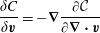 $$\begin{eqnarray}\frac{\unicode[STIX]{x1D6FF}C}{\unicode[STIX]{x1D6FF}\boldsymbol{v}}=-\unicode[STIX]{x1D735}\frac{\unicode[STIX]{x2202}{\mathcal{C}}}{\unicode[STIX]{x2202}\unicode[STIX]{x1D735}\boldsymbol{\cdot }\boldsymbol{v}}\end{eqnarray}$$
 and, as is evident from (4.64), that  $\unicode[STIX]{x1D735}\boldsymbol{\cdot }({\mathcal{P}}_{\unicode[STIX]{x1D70C}}\unicode[STIX]{x1D735}\unicode[STIX]{x1D6F7})=0$ for all $\unicode[STIX]{x1D6F7}$; hence, all the $\unicode[STIX]{x1D6FF}C/\unicode[STIX]{x1D6FF}\boldsymbol{v}$ terms vanish except the first term of the last line of (4.69). This term combines with the others to cancel, just as for the calculation of $\hat{{\mathcal{C}}}$.
For constant density, entropy and magnetic field, the bracket of (4.77) reduces to
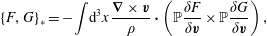 $$\begin{eqnarray}\{F,G\}_{\ast }=-\int \text{d}^{3}x\,\frac{\unicode[STIX]{x1D735}\times \boldsymbol{v}}{\unicode[STIX]{x1D70C}}\boldsymbol{\cdot }\left(\mathbb{P}\frac{\unicode[STIX]{x1D6FF}F}{\unicode[STIX]{x1D6FF}\boldsymbol{v}}\times \mathbb{P}\frac{\unicode[STIX]{x1D6FF}G}{\unicode[STIX]{x1D6FF}\boldsymbol{v}}\right),\end{eqnarray}$$
whence it is easily seen that the helicity
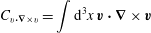 $$\begin{eqnarray}C_{v\boldsymbol{\cdot }\unicode[STIX]{x1D735}\times v}=\int \text{d}^{3}x\,\boldsymbol{v}\boldsymbol{\cdot }\unicode[STIX]{x1D735}\times \boldsymbol{v}\end{eqnarray}$$
 is a Casimir invariant because  $\mathbb{P}\,(\unicode[STIX]{x1D735}\times \boldsymbol{v})=\unicode[STIX]{x1D735}\times \boldsymbol{v}$. This Casimir is lost when entropy and density are allowed to be advected, for it is no longer a Casimir invariant of (4.69).
Now, let us consider invariants in the Lagrangian description. Without the incompressibility constraints, the Hamiltonian has a standard kinetic energy term and the internal energy depends on  $\unicode[STIX]{x2202}q/\unicode[STIX]{x2202}a$, an infinitesimal version of the two-body interaction, if follows that just like the $N$-body problem the system has Galilean symmetry, and because the Poisson bracket in the Lagrangian description (3.15) is canonical there are no Casimir invariants. With the incompressibility constraint, the generators of the algebra now respect the constraints, with Dirac constraints being Casimirs and the algebra of constraints now having a non-trivial centre. Because the Casimirs are pointwise invariants, we expect the situation to be like that for the Maxwell Vlasov equation (Morrison Reference Morrison1982), where the following is a Casimir:
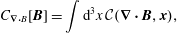 $$\begin{eqnarray}C_{\unicode[STIX]{x1D735}\boldsymbol{\cdot }B}[\boldsymbol{B}]=\int \text{d}^{3}x\,{\mathcal{C}}(\unicode[STIX]{x1D735}\boldsymbol{\cdot }\boldsymbol{B},\boldsymbol{x}),\end{eqnarray}$$
 with  ${\mathcal{C}}$ being an arbitrary function of its arguments. Because both $\unicode[STIX]{x1D735}\boldsymbol{\cdot }\boldsymbol{B}$ and ${\mathcal{J}}$ are pointwise constraints, analogous to (4.110) we expect the following Casimir:
 $$\begin{eqnarray}{\hat{C}}[{\mathcal{J}}]=\int \text{d}^{3}a\,\hat{{\mathcal{C}}}({\mathcal{J}},\boldsymbol{a}).\end{eqnarray}$$
 Indeed, only the first term of (4.52) contributes when we calculate  $\{{\hat{C}},G\}_{\ast }$ and this term vanishes by (4.49) because
 $$\begin{eqnarray}\frac{\unicode[STIX]{x1D6FF}{\hat{C}}}{\unicode[STIX]{x1D6FF}q^{i}}=-\frac{\unicode[STIX]{x2202}}{\unicode[STIX]{x2202}a^{\ell }}\left(A_{i}^{\ell }\frac{\unicode[STIX]{x2202}\hat{{\mathcal{C}}}}{\unicode[STIX]{x2202}{\mathcal{J}}}\right),\end{eqnarray}$$
which follows upon making use of (3.7). Similarly, it can be shown that the full Casimir is
 $$\begin{eqnarray}{\hat{C}}[D^{1},D^{2}]=\int \text{d}^{3}a\,\hat{{\mathcal{C}}}(D^{1},D^{2},\boldsymbol{a}),\end{eqnarray}$$
a Lagrangian Casimir consistent with (4.106).
For MHD, the magnetic helicity,
 $$\begin{eqnarray}C_{A\boldsymbol{\cdot }B}=\int \text{d}^{3}x\,\boldsymbol{A}\boldsymbol{\cdot }\boldsymbol{B},\end{eqnarray}$$
 where  $\boldsymbol{B}=\unicode[STIX]{x1D735}\times \boldsymbol{A}$ is easily seen to be preserved and a Casimir up to the usual issues regarding gauge conditions and boundary terms (see Finn & Antonsen Reference Finn and Antonsen1985). We know that the cross-helicity
 $$\begin{eqnarray}C_{v\boldsymbol{\cdot }B}=\int \text{d}^{3}x\,\boldsymbol{v}\boldsymbol{\cdot }\boldsymbol{B},\end{eqnarray}$$
is a Casimir of the compressible barotropic MHD equations, and it is easy to verify that it is also a Casimir of (4.77) added to (4.78), that is for uniform density. However, it is not a Casimir for the case with advected density, i.e. for the bracket of (4.69) added to (4.70).
5 Conclusions
In this paper we have substantially investigated constraints, particularly incompressibility for the ideal fluid and MHD, for the three dichotomies described in § 1.1: the Lagrangian versus Eulerian fluid descriptions, Lagrange multiplier versus Dirac constraint methods and Lagrangian versus Hamiltonian formalisms. An in depth description of the interplay between the various fluid and MHD descriptions was given, with an emphasis on Dirac’s constraint method. Although we mainly considered geodesic flow for simplicity, the Dirac’s Poisson bracket method can be used to find other forces of constraint in a variety of fluid and plasma contexts.
Based on our results, many avenues for future research are presented. We mention a few. Since the Hamiltonian structure of extended and relativistic MHD are now at hand (Charidakos et al. Reference Charidakos, Lingam, Morrison, White and Wurm2014; Abdelhamid, Kawazura & Yoshida Reference Abdelhamid, Kawazura and Yoshida2015; D’Avignon, Morrison & Pegoraro Reference D’Avignon, Morrison and Pegoraro2015; D’Avignon, Morrison & Lingam Reference D’Avignon, Morrison and Lingam2016; Lingam, Miloshevich & Morrison Reference Lingam, Miloshevich and Morrison2016; Kaltsas, Throumoulopoulos & Morrison Reference Kaltsas, Throumoulopoulos and Morrison2020) calculations analogous to those presented here can be done for a variety of magnetofluid models. Another valuable class of models that could be studied, ones that are known to have Lagrangian and Hamiltonian structure, are those with various finite-Larmor-radius effects (e.g. Tassi et al. Reference Tassi, Morrison, Waelbroeck and Grasso2008; Izacard et al. Reference Izacard, Chandre, Tassi and Ciraolo2011; Tassi Reference Tassi2014, Reference Tassi2019).
Another avenue for future research would be to address stability with constraints. In a previous series of papers (Andreussi, Morrison & Pegoraro Reference Andreussi, Morrison and Pegoraro2010, Reference Andreussi, Morrison and Pegoraro2012, Reference Andreussi, Morrison and Pegoraro2013, Reference Andreussi, Morrison and Pegoraro2015, Reference Andreussi, Morrison and Pegoraro2016) we have investigated Hamiltonian based stability, generalizations of the MHD energy principle or the ideal fluid Rayleigh criterion, within the Lagrangian, energy-Casimir, and dynamically accessible frameworks. Because Dirac’s method adds Casimirs, the Dirac constraints, one gets a richer set of equilibria from the energy-Casimir variational principle and these can be tested for Lyapunov stability. Similarly, the method of dynamical accessibility (see Morrison Reference Morrison1998) based on constrained variations induced by the Poisson operator will enlarge the set of stable equilibria.
Recently there has been consider research in the development of structure preserving computational algorithms (see, e.g. Morrison (Reference Morrison2017) for review). These are algorithms that preserve various geometric, Hamiltonian, variational and other structure of fluid, kinetic and other physical models. In the plasma community, in particular, we mention Evstatiev & Shadwick (Reference Evstatiev and Shadwick2013), Qin et al. (Reference Qin, Liu, Xiao, Zhang, He, Wang, Burby, Ellison and Zhou2016), Xiao et al. (Reference Xiao, Qin, Morrison, Liu, Yu, Zhang and He2016) and Kraus et al. (Reference Kraus, Kormann, Morrison and Sonnendrücker2017), but there is a large body of additional work by these and other authors. Given how the finite-dimensional material of § 2 so strongly parallels the infinite-dimensional material of § 4, notably the structure of geodesic flow, a natural avenue for future research would be to develop numerical algorithms that preserve this structure.
Lastly, we mention that there is considerable geometric structure behind our calculations that could be further developed. Our results can be restated in geometric/Lie group language (see e.g. Bloch (Reference Bloch2002)). Also, Arnold’s program for obtaining the Riemann curvature for geodesic flow on the group of volume preserving diffeomorphisms can be explored beginning from our results of § 4. We did not feel this special issue would be the appropriate place to explore these ideas.
Acknowledgements
P.J.M. was supported by U.S. Dept. of Energy under contract #DE-FG02-04ER-54742. He would also like to acknowledge support from the Humboldt Foundation and the hospitality of the Numerical Plasma Physics Division of the IPP, Max Planck, Garching. F.P. would like to acknowledge the hospitality of the Institute for Fusion Studies of the University of Texas at Austin.
