


1. Introduction
The fundamental observation equation in a global navigation satellite system (GNSS) is

where $t_{i}$ is the observed (estimated) time of arrival of a code from satellite $i$
 , $t_{D,i}$
 is the time of departure of the signal, $c$
 is the speed of light, $\mathring {\ell }$
 is the location of the receiver, $\rho _{i}(t_{D,i})$
 is the location of the satellite at the time of transmission, $\mathring {b}$
 is the offset in time-of-arrival observation caused by the inaccurate clock at the receiver and by delays in the analogue radio-frequency (RF) chain (e.g. in cables), $\delta _{i}$
 represents atmospheric delays and the satellite's clock error, and $\epsilon _{i}$
 is an error or noise term that accounts for both physical noise and for unmodelled effects. Normally, the GNSS solver estimates $\mathring {\ell }$
 and $\mathring {b}$
 by minimising the norm of the error vector $\epsilon$
 ; it does not know $\epsilon _{i}$
 and does not attempt to estimate it. The quantities $t_{D,i}$
 and $\rho _{i}(t_{D,i})$
 are usually known; $t_{D,i}$
 is known because the satellite timestamps its transmission, and $\rho _{i}(t_{D,i})$
 is known because the satellite transmits the parameters that define its orbit, called the ephemeris. The ephemeris can also be downloaded from the Internet.
Decoding $t_{D,i}$ takes a significant amount of time, in a global positioning system (GPS) up to 6 s under good signal-to-noise ratio (SNR) conditions and longer in low-SNR conditions. GNSS receivers that need to log locations by observing the RF signals for short periods cannot decode $t_{D,i}$
 . Examples for such applications include tracking marine animals like sea turtles, which surface briefly and then submerge again. It turns out that techniques that are collectively called snapshot positioning or coarse-time navigation can estimate $\mathring {\ell }$
 and $\mathring {b}$
 when $t_{D,i}$
 is not known. These techniques can also reduce the time to a first fix when a receiver is turned on.
Snapshot receivers sample the incoming GNSS RF signals for a short period, called a snapshot. Usually (but not always), the RF samples are correlated with replicas of the codes transmitted by the satellites, therefore determining $t_{i}$ for the subset of visible satellites. The correlation (and Doppler search) is sometimes performed on the receiver, which then stores or transmits the $t_{i}$
 data. This appears to be the case for a proprietary technology called Fastloc, which is used primarily to track marine animals (Tomkiewicz et al., Reference Tomkiewicz, Fuller, Kie and Bates2010; Witt et al., Reference Witt, Åkesson, Broderick, Coyne, Ellick, Formia, Hays, Luschi, Stroud and Godley2010; Dujon et al., Reference Dujon, Lindstrom and Hays2014). In other cases (Ramos et al., Reference Ramos, Zhang, Liu, Priyantha, Kansal, Patterson, Rogers and Xie2011; Bavaro, Reference Bavaro2012a, Reference Bavaro2012b; Liu et al., Reference Liu, Priyantha, Hart, Ramos, Loureiro, Wang, Campbell and Langendoen2012; Cvikel et al., Reference Cvikel, Berg, Levin, Hurme, Borissov, Boonman, Amichai and Yovel2015; Eichelberger et al., Reference Eichelberger, von Hagen, Wattenhofer and Zhong2019; Harten et al., Reference Harten, Katz, Goldshtein, Handel and Yovel2020), the logger records the raw RF samples and correlation is performed after the data are uploaded to a computer.
Techniques for estimating $\mathring {\ell }$ when the $t_{D,i}$
 data are not known date back to a paper by Peterson et al. (Reference Peterson, Hartnett and Ottman1995). They proposed to view $t_{D,i}$
 as a function of both $t_{i}$
 and a coarse clock-error unknown that they call coarse time, which in principle is identical to $\mathring {b}$
 , but is modelled by a separate variable. They then showed that it is usually possible to estimate $\mathring {\ell }$
 , $\mathring {b}$
 and the coarse time from five or more $t_{i}$
 points. This method does not always resolve the $t_{D,i}$
 correctly. Lannelongue and Pablos (Reference Lannelongue and Pablos1998) and Van Diggelen (Reference Van Diggelen2002, Reference Van Diggelen2009) proposed methods that appear to always resolve the $t_{D,i}$
 correctly when the initial estimate of $\mathring {\ell }$
 and $\mathring {b}$
 are within some limits (adding up to approximately 150 km). Muthuraman et al. (Reference Muthuraman, Brown and Chansarkar2012) showed that the two methods are equivalent in the sense that they usually produce the same estimates. However, the method of Lannelongue and Pablos is an iterative search procedure, while Van Diggelen's is a rounding procedure that is more computationally efficient, so Van Diggelen's method became much more widely used and widely cited. Van Diggelen also showed how to use an iterative procedure over a number of possible positions when the initial estimate of $\mathring {\ell }$
 and $\mathring {b}$
 is outside the 150 km limit.
All three methods use a system of linearised equations with five scalar unknowns (not the usual four), which are corrections to the coordinates of $\mathring {\ell }$ , the offset $\mathring {b}$
 (which he refers to as the common bias) and the coarse time unknown, usually denoted by $tc$
 (we denote it in this paper by the single letter $s$
 ).
).
Van Diggelen's algorithm was used and cited in numerous subsequent papers, all of which repeat his presentation without adding explanations. Liu et al. (Reference Liu, Priyantha, Hart, Ramos, Loureiro, Wang, Campbell and Langendoen2012), Ramos et al. (Reference Ramos, Zhang, Liu, Priyantha, Kansal, Patterson, Rogers and Xie2011) and Wang et al. (Reference Wang, Qin and Jin2019) describe snapshot GPS loggers whose recordings are processed using the algorithm. Badia-Solé and Iacobescu Ioan (Reference Badia-Solé and Iacobescu Ioan2010) report on the performance of the method. Othieno and Gleason (Reference Othieno and Gleason2012), Chen et al. (Reference Chen, Wang, Chiang and Chang2014) and Fernández-Hernández and Borre (Reference Fernández-Hernández and Borre2016) show how to use Doppler measurements to obtain an initial estimate that satisfies the requirements of Van Diggelen's algorithm. Yoo et al. (Reference Yoo, Kim, Lee and Lee2020) propose a technique that replaces the estimation of the coarse-time parameter by a one-dimensional search, which allows them to estimate $\mathring {\ell }$ using observations from four satellites, but at considerable computational expense.
Bissig et al. (Reference Bissig, Eichelberger, Wattenhofer, Dutta and Xing2017) use a direct position determination (Weiss, Reference Weiss2004) approach to snapshot positioning. They quantise the four unknowns $\mathring {\ell }$ and $\mathring {b}$
 , and maximise the likelihood of the received snapshot over this four-dimensional lattice. To make the search efficient, they use a branch and bound approach that prunes sets of unlikely solutions. It appears that this approach allows them to estimate locations using very short snapshots, but at the cost of fairly low accuracy and relatively long running times, compared with methods that estimate the $t_{i}$
 data first.
In this paper we derive the observation equations that underlie the methods of Peterson et al. (Reference Peterson, Hartnett and Ottman1995), Lannelongue and Pablos (Reference Lannelongue and Pablos1998) and Van Diggelen (Reference Van Diggelen2002, Reference Van Diggelen2009). These authors show the correction equations, not the observation equations whose Jacobian constitutes the correction equations. The formulation of the observation equations, which constitute a mixed-integer least-squares problem, allows us to apply a new type of algorithm to estimate the integer unknowns. A mixed-integer least-squares problem is an optimisation problem with a least-squares objective function and both real (continuous) unknowns and integer unknowns. More specifically, we regularise the mixed-integer problem using either a priori estimates of $\mathring {\ell }$ and $\mathring {b}$
 or Doppler-shift observations. Our approach is inspired by the real-time kinematic (RTK) method, which resolves a position from both code-phase and carrier-phase GNSS observations (Teunissen, Reference Teunissen, Teunissen and Montenbruck2017); carrier-phase constraints have integer ambiguities that must be resolved.
Our experimental results using real-world data demonstrate that our new algorithms can resolve locations with much larger initial location and time errors than the method of Van Diggelen. Van Diggelen's non-iterative method only works when the initial estimate is up to approximately 150 km (or equivalent combinations), whereas our mixed-integer least-squares solver works with initial errors of up 150 s and 200 km. When using Doppler-shift regularisation, our method works even with initial errors of 180 s and arbitrarily large initial position errors (on Earth); if the initial position error is small, the method tolerates initial time errors of up to 5000 s.
Our implementation of the new methods and the code that we used to evaluate them are publicly available.Footnote 1
The rest of this paper is organised as follows. Section 2 presents the observation equations for the snapshot-positioning GNSS problem. Section 3 explains how to incorporate the so-called coarse-time parameter into the observation equations and how Van Diggelen's method exploits it. Section 4.1 presents our first regularised formulation, which uses the initial guess to regularise the mixed-integer least-squares problem. Section 4.2 presents the Doppler-regularised formulation. Our experimental results are presented in Section 5. Section 6 discusses our conclusions from this research.
2. The snapshot-positioning problem: a GNSS model with whole-millisecond ambiguities
We begin by showing that when departure times are not known, the observation equations that relate the arrival times of GNSS codes to the unknown position of the receiver contain integer ambiguities.
We denote by $t_{D,i}$ the time of departure of a code from satellite $i$
 , and we assume that $t_{D,i}$
 represents a whole millisecond (in the time base of the GPS system). We denote by $\mathring{t}_{i}$
 the time of arrival of that code at the antenna of the receiver. We assume that the receiver estimates the arrival time of that code as $t_{i}=\mathring{t}_{i}+\mathring {b}+\epsilon _{i}$
 , where $\mathring {b}$
 represents the bias that is caused by the inaccurate clock of the receiver and by delays that the signal experiences in the path from the antenna to the analogue-to-digital converter, and $\epsilon _{i}$
 is the arrival-time estimation error. The bias $\mathring {b}$
 is time dependent, because of drift in the receiver's clock, but over short observation periods this dependence is negligible, so we ignore it.
The time of arrival is governed by the equation

where $c$ is the speed of light, $\mathring {\ell }$
 is the location of the receiver, $\rho _{i}$
 is the location of the satellite (which is a function of time, since the satellites are not stationary relative to Earth observers), and $\delta _{i}$
 represents the inaccuracy of the satellite's clock and atmospheric delays. We assume that $\delta _{i}$
 can be modelled, for example using models of ionospheric and tropospheric delays (dual frequency receivers can estimate the ionospheric delay, but we assume a single-frequency receiver). Setting $\delta _{i}$
 to the satellite's clock error correction from the ephemeris induces a location error of approximately 30 m due to the atmospheric delays (Borre and Strang, Reference Borre and Strang2012).
A receiver that decodes the timestamp embedded in the GPS data stream can determine $t_{D,i}$ , which leads to the following equation:

the conventional GNSS code-observation equation, in which the four unknown parameters are $\mathring {b}$ and the coordinates of $\mathring {\ell }$
 (we assume that $\delta _{i}$
 is modelled, possibly trivially $\delta _{i}=0$
 , but not estimated). To simplify the notation, we ignore $\delta _{i}$
 for now and write

We use observations from all the satellites such that all the $t_{i}$ data lie between two consecutive whole multiples of $t_{\text {code}}$
 (in GPS, two round milliseconds in the local clock). This allows us to express

with a common and easily computable $N=\lfloor t_{i}/t_{\text {code}}\rfloor$ and for $\varphi _{i}\in [0,1)$
 . We denote $N_{i}=t_{D,i}/t_{\text {code}}$
 and write

Since GNSS codes are aligned with $t_{\text {code}},$ $N_{i}\in \mathbb {Z}$
 . We denote $n_{i}=N-N_{i}\in \mathbb {Z}$
 , so
, so

or

We now face two challenges. One is that we have $4+m$ unknown parameters: three location coordinates, $\mathring {b}$
 and $n_{i}$
 , but only $m$
 constraints. We clearly need more constraints so that we can resolve $n_{i}$
 . The other is that we have a set of nonlinear constraints with continuous real unknowns, the location and $\mathring {b}$
 , and with integer unknowns, the $n_{i}$
 . The strategy, as in other cases with this structure, is to first linearise the nonlinear term, then to resolve the integer parameters, and to then substitute them and to solve the continuous least-squares problem (either the linearised system or the original nonlinear system). We cannot linearise the nonlinear term $\|\mathring {\ell }-\rho _{i}(t_{D,i})\|_{2}/c$
 using a Taylor series because it is a function of both real unknowns and of the integer unknowns $n_{i}$
 . We cannot differentiate this term with respect to the integer $n_{i}$
 .
.
To address this difficulty, we approximate $t_{D,i}$ by approximating the range (distance) term in the equation

For now, we denote the approximation of the propagation delay by

so

There are several ways to set $d_{i}$ , depending on our prior knowledge of $\mathring {\ell }$
 and $\mathring {b}$
 . One option in the GPS system is to set it to approximately 76$\cdot$
 5 ms; this limits the error in $\hat {t}_{D,i}$
 to approximately 12$\cdot$
 5 ms for any Earth observer, and the error

to approximately 10 m (Van Diggelen, Reference Van Diggelen2009). We substitute $\rho _{i}(\hat{t}_{D,i})=\rho _{i}(t_{i}-d_{i}-\mathring {b})$ for $\rho _{i}(t_{D,i})$
 ,
,

The superscript $(D)$ on the error term indicates that the error term now represents not only the arrival-time estimation error, but also the error induced by the inexact departure time.
We linearise around an a priori solution $\bar {\ell }$ and $\bar {b}$
 (usually $\bar {b}=0$
 , otherwise we can simply shift the $t_{i}$
 s),
s),

where $\mathrm {J}$ is the Jacobian of the Euclidean distances with respect to both the location of the receiver and to the bias, with the derivatives evaluated at $\bar {\ell }$
 and at $t_{i}-d_{i}-\bar {b}$
 . The superscript $(D,L)$
 on the error term indicates that it now includes also the linearisation error.
There are now several ways to resolve the $n_{i}$ .
.
3. Shadowing
Peterson et al. (Reference Peterson, Hartnett and Ottman1995) introduced a somewhat surprising modelling technique, which we refer to as shadowing. The idea is to replace the unknown $b$ by two separate unknowns that represent essentially the same quantity, the original $b$
 and a shadow $s$
 . In principle, they should obey the equation $b=s$
 , but the model treats $s$
 as a free parameter; the constraint $b=s$
 is dropped. In the literature, $s$
 is called the coarse-time parameter (and is often represented by $tc$
 or $t_{c}$
 ). We express this technique by splitting $b$
 and $s$
 :
:

We now have five unknowns, not four.
As far as we can tell, there is no clear explanation in the literature as to the benefits of shadowing. One way to justify the technique is to observe that Equation (2.2) is very sensitive to small (nanosecond scale) perturbations in the additive $\mathring {b}$ , but it is not highly sensitive to the $\mathring {b}$
 (now $s$
 ) by which we multiply,

For example, in GPS, the derivative is bounded by approximately $800$ m/s for any $\bar {\ell }$
 on Earth (Van Diggelen, Reference Van Diggelen2009), so $\mathrm {J}_{i,4}/c<3\times 10^{-6}$
 (versus $1$
 for the additive $\mathring {b}$
 ). Therefore, the dependence of the residual (the vector of $\epsilon _{i}^{(D,L)}$
 terms for a given setting of the unknown parameters) on $\mathring {b}$
 in Equation (2.2) is highly non-convex. There are many different values of $\mathring {b}$
 that are almost equally good, a millisecond apart, with each of these nearly optimal hypotheses being locally well defined; if we increase $\mathring {b}$
 by one millisecond and also add $1$
 to each $n_{i}$
 , the residual changes very little, because $\mathrm {J}{}_{i,4}$
 is so small.
Shadowing turns this non-convexity into explicit rank deficiency, with which it is easier to deal. With one instance of $\mathring {b}$ replaced by the shadow $s$
 , the constraints no longer uniquely define $\mathring {b}$
 , only up to a multiple of $t_{\text {code}}$
 . For any hypothetical solution $\ell ,s,b,n$
 , the solution $\ell ,s,b+kt_{\text {code}},n+k$
 gives exactly the same residual. We perform a change of variables, replacing the partial sum $-n_{i}t_{\text {code}}+\mathring{b}$
 by $-\nu _{i}t_{\text {code}}+\beta$
 , where $-\nu _{i}=-n_{i}+\lfloor \mathring{b}/t_{\text {code}}\rfloor$
 and $\beta =\mathring {b}-\lfloor b/t_{\text {code}}\rfloor t_{\text {code}}$
 , so $\beta \in [0,t_{\text {code}})$
 :
:

3.1 Resolving the integer ambiguities: Van Diggelen's method
Van Diggelen's method exploits the fact that the $\nu _{i}$ values are very insensitive to $\mathring {\ell }$
 and to $s$
 . It therefore sets $\mathring {\ell }=\bar {\ell }$
 and $s=\bar {b}$
 , truncating the Jacobian term from Equation (3.2):

The new subscript $(D,L,A)$ indicates that the error term now compensates also for the use of the a priori estimates $\bar {b}$
 and $\bar {\ell }$
 for $s$
 and $\mathring {\ell }$
 .
.
Van Diggelen uses these constraints to set the $\nu _{i}$ values in a particular way. The method selects one index $j$
 that is used to set $\nu _{j}$
 and $\beta$
 , and then resolves all the other $\nu _{i}$
 values so they are consistent with this $\beta$
 . That is, he assumes that $\epsilon _{j}^{(D,L,A)}=0$
 so
so

The method now substitutes this $\beta$ in all the other constraints and assigns the other $\nu _{i}$
 values by setting $\epsilon _{i}^{(D,L,A)}=0$
 and rounding,

When $\|\mathring {\ell }-\bar {\ell }\|$ and $|s-\bar {b}|$
 are small enough, this gives a set of $\nu _{i}$
 values that are correct in the sense that they all differ from the correct $\nu _{i}$
 values by the same integer.
Van Diggelen chooses $j$ in a particular way: he chooses the $j$
 that minimises the magnitude of Equation (3.1), which corresponds to the satellite closest to the zenith of $\bar {\ell }$
 at $t_{j}-\bar {b}$
 . In our notation, Van Diggelen's justification for this choice is as follows. He searches for a $j$
 for which Equation (3.3) approximates well Equation (3.2). The difference between the two is

For each satellite, $\mathrm {J}_{i,1:3}$ is the negation of the so-called line-of-sight vector $e_{i}^{T}$
 , which is the normalised direction from the satellite to the receiver; element $\mathrm {J}_{i,4}$
 is the range rate. Van Diggelen's choice of $j$
 leads to a row of $\mathrm {J}$
 in which the first three elements are almost orthogonal to $\mathring {\ell }-\bar {\ell }$
 and in which the fourth element, the range rate, is small. This leads to an estimated $\beta$
 that is relatively accurate, which helps resolve the correct $\nu _{i}$
 values.
Van Diggelen also shows that if we resolve the $\nu _{i}$ values by setting each $\epsilon _{i}^{(D,L,A)}=0$
 separately, then the resolved $\beta$
 values might be close to $0$
 in one equation and close to $t_{\text {code}}$
 in another; this leads to inconsistent $\nu _{i}$
 values and to a huge position error.
3.2 Final resolution of the receiver's location
Van Diggelen's method resolves the integer $\nu _{i}$ values in Equation (3.3). Now we need to resolve the continuous unknowns. We do so using Gauss–Newton iterations on Equation (3.2), iterating on $\delta _{\ell }=\mathring {\ell }-\bar {\ell }$
 , $\delta _{s}=s-\bar {b}$
 and $\beta$
 but keeping $\nu$
 fixed. We start with $\delta _{\ell }$
 , $\delta _{s}$
 and $\beta$
 set to zero.
In every iteration, we use the current iterates to produce estimates of the location and bias,

We use them to improve the estimate of the ranges $d_{i}$ , setting

This allows us to reduce the errors in Equation (2.1),

(the second line holds because $n_{i}t_{\text {code}}+\mathring {b}=\nu _{i}t_{\text {code}}+\beta$ , by definition). We again linearise this and solve the constraints

for $\mathring {\ell }$ , $s$
, $s$ and $\beta$
 using in the generalised least-squares sense, where the Jacobian is evaluated at $\hat {\ell }$
 and $t-\hat {d}-\hat {b}$
 .
.
We can now explain why Van Diggelen's method resolves the integers only once and iterates only on the continuous unknowns. The $\nu _{i}$ values that Van Diggelen's method resolves are not equal to the $n_{i}$
 values in the nonlinear Equation (2.1). But when the linearisation error is small enough, the two integer vectors differ by a constant, $\lfloor \mathring{b}/t_{\text {code}}\rfloor$
 . This difference is compensated for by the integer part of the continuous variable $\beta$
 , which is not constrained to $[0,t_{\text {code}})$
 in the Gauss–Newton iterations. This is the actual function of shadowing; to allow $\beta$
 to compensate not only for the clock error, but also for the constant error in $\nu$
 . When the initial linearisation error is so large that $n-\nu$
 is no longer a constant, the method breaks down.
4. A mixed-integer least-squares approach
A different approach, which has never been proposed for snapshot positioning, is to add regularisation constraints that will allow us to resolve all the $4+m$ unknowns in the $m$
 instances of Equation (2.2)

using mixed-integer least-squares techniques. Note that we have rewritten Equation (2.2) in a way that emphasises a change of variables that facilitate iterative improvements: the new unknowns are $\mathring {\ell }-\bar {\ell }$ , $\mathring {b}-\bar {b}$
 and $\mathring {n}-\bar {n}$
 . We initially set $\bar {b}$
 and $\bar {n}$
 to zero.
We denote the vector of delays by $g$ ,
,

This section proposes two sets of regularising equations and explains how to use this approach in an iterative Gauss–Newton solver.
4.1 Resolving the ambiguities: regularisation using a priori estimates
The first set of regularising equations that we propose are

We do not enforce them exactly, only in a (weak) least-squares sense. They favour solutions of the mixed-integer least-squares problem that are in the vicinity of the a priori solution. This leads to the following weighted mixed-integer least-squares problem:

where $W$ is a block-diagonal weight matrix derived from the covariance matrix $C$
 of the error terms $\epsilon$
 , $W^{T}W=C^{-1}$
 . Now we have $2m$
 constraints, which for $m\geq 4$
 should allow us to resolve the integer $n_{i}$
 values.
We propose to choose a diagonal $W$ as follows. We set the first $m$
 diagonal elements of $W$
 to the standard deviation of the arrival-time estimator, say $W_{i,i}=1/\sigma (t_{i})\approx 1/(10\,\text {ns})$
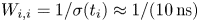 . To set the rest, we use box constraints on the a priori estimates $\bar {\ell }$
 and $\bar {b}$
 , denoted as

By the triangle inequality

We define

so

We convert the hard box constraints into soft-weighted least-squares in order to allow for using a mixed-integer least-squares solver. We need to set $W_{m+i,m+i}$ ; if we assume that the error in the constraint is Gaussian and that an error of $r_{i}/c$
 is acceptable (from the inequality above), then setting $W_{m+i,m+i}=c/r_{i}$
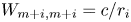 , say, makes sense. In practice, we use $W_{m+i,m+i}=c/(100\,\text {km})$
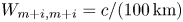 in the experiments below.
This mixed-integer least-squares minimisation problem can be solved by a generic solver, such as one of the solvers that have been developed for RTK.
4.2 Doppler regularisation
It turns out that Doppler shifts allow us to regularise Equation (2.2) in a more effective way. GNSS receivers estimate not only the time of arrival of the signal, but also its Doppler shift. The estimated Doppler shift is biased, because of the inaccuracy of the receiver's local (or master) oscillator; it is also inexact. We now show a novel technique to use the Doppler-shift observations to to regularise Equation (2.2).
Our technique is based on two assumptions. One is that the receiver is stationary, or more precisely, that its velocity is negligible relative to the range rate, which is up to approximately 800 m/s. This assumption can be easily removed, but its removal leads to additional unknowns and more complicated expressions that we do not present here. The other assumption is that the local oscillator and the sampling clock in the receiver are derived from a single master oscillator in a certain (very common) way. Again, this assumption can be removed if another unknown is added.
The Doppler-shift formula for velocities much lower than the speed of light is

The Doppler observations that the receiver makes are

where $\mathring {f}$ is the frequency offset (bias) of the receiver and $\epsilon _{i}^{(\delta )}$
 is an error term that represents the observation error and the (negligible) slow-speed approximation. Therefore, the quantities $-cD_{i}/f_{0}$
 are biased estimates of the range rate. We denote the a priori estimates of the Doppler shifts by $\bar {D}_{i}$
 .
.
We differentiate Equation (2.2) by time,

We first manipulate the equation a little, to make it easier to differentiate:

We denote

The first three columns of $H$ are identical to those of $\mathrm {J}$
 , the next is the fourth column of $\mathrm {J}$
 but shifted by $c$
 and the last $m$
 columns consist of a scaled identity matrix. We now express the derivative on the right-hand side of Equation (4.2) as

We assume that the receiver is stationary, so $\mathring {\ell }-\bar {\ell }$ is time-independent, so $({d}/{dt})(\mathring {\ell }-\bar {\ell })=0$
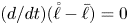 . The derivatives of the integers $n_{1},\ldots ,n_{m}$
 are also zero. The derivative of the remaining element in the vector, $({d}/{dt})(\mathring {b}-\bar {b})$
 , is not zero and will need to be estimated. It represents the frequency offset of the receiver, which biases the observed Doppler shift. It is multiplied by a column whose elements are very close to $c$
 (the range rate is tiny relative to the speed of light), which allows it to compensate for the frequency bias.
To differentiate $H$ , we exploit the known structure of $\mathrm {J}$
 . For each satellite, $\mathrm {J}_{i,1:3}$
 is the negation of the so-called line-of-sight vector $e_{i}^{T}$
 , which is the normalised direction from the satellite to the receiver; element $\mathrm {J}_{i,4}$
 is the range rate. The derivatives of these quantities are shown by Van Diggelen (Reference Van Diggelen2009, Equation 8.6), Fernández-Hernández and Borre (Reference Fernández-Hernández and Borre2016) and other sources:

where the satellite position $\rho _{i}$ and its velocity $({d}/{dt})\rho _{i}$
 are taken at $\hat {t}_{D}$
 . To reduce the number of unknowns, we assume that the receiver is stationary, so $({d}/{dt})\bar {\ell }=0$
 , so
, so

Element $\mathrm {J}_{i,4}$ is the range rate of satellite $i$
 , so its derivative with respect to time is the satellite's range acceleration,

We use finite differences to evaluate this second derivative. The fourth column of $H$ is $\mathrm {J}_{:,4}+c$
 , but the derivative of $c$
 is obviously zero. The derivative of $-ct_{\text {code}}$
 is also zero, so

We now derive the left-hand side of Equation (4.2),

The derivative of the a prioi range estimate $\Vert \bar {\ell }-\rho _{i}(t_{i}-d_{i}-\bar {b})\Vert _{2}$ is the a priori range rate, which we can compute. The derivative of $c\bar {b}$
 is zero.
To understand the first term, recall that

so

We now rewrite Equation (4.1) as

or

We now substitute in the left-hand side of Equation (4.2):

The term $\mathring {f}/f_{0}$ is the relative local-oscillator error in the receiver. If the oscillator runs too fast, $\mathring {f}$
 is negative. Assuming that all the clocks in the receiver are derived from a master oscillator, if it runs too fast, $\mathring {b}$
 grows over time. Under this assumption,

so these terms cancel each other. If our assumption on the receiver does not hold, we would need to estimate

We have arrived at a system of $m$ linear equations that we use to regularise the mixed-integer equations. The equations are:

In this equation, $D$ represents the vector of observed Doppler shifts, $({d}/{dt})\Vert \mathring {\ell }-\rho \Vert _{2}$
 is the vector of the a priori range rates and $\mathring {u}-\bar {u}=({d}/{d\,t})(\mathring {b}-\bar {b})$
 is a new scalar unknown. We have explained above how to compute $H_{:,4}$
 and $({d}/{dt})H_{:,1:4}$
 . The full regularised weighted least-squares that we solve is

4.3 Iterating to cope with large a priori errors
Solving the linearised and regularised mixed-integer least-squares problem improves the initial a priori estimates of $\mathring {\ell }$ and $\mathring {b}$
 , but not to the extent possible given the code phases. The most important factor that limits the accuracy of the corrections is the fact that when the a priori estimates are large, the resolved integers, the $n_{i}$
 values, are inexact. Therefore, we incorporate the mixed-integer solver into a Gauss–Newton-like iteration in which we correct all the unknowns, including the integer ambiguities, more than once.
More specifically, once we solve the mixed-integer least-squares problem for $\mathring {n}-\bar {n}$ , $\mathring {\ell }-\bar {\ell }$
 and $\mathring {b}-\bar {b}$
 (and for $\mathring {u}-\bar {u}$
 in the Doppler formulation), we use the corrections to improve the estimates of the receiver's location and of the departure times, and we linearise Equation (2.1) again. We now solve the newly linearised least-squares problem again for additional corrections, and so on.
5. Implementation and evaluation
We have implemented all the methods that we described above in MATLAB.
We use Borre's Easy Suite (Borre, Reference Borre2003, Reference Borre2009) to perform many routine calculations. In particular, we use it to correct the GPS time (check_t), to correct for Earth rotation during signal propagation time (e_r_corr), to read an ephemeris from a RINEX file and to extract the data for a particular satellite (rinexe, get_eph and find_eph), to transform Julian dates to GPS time (gps_time), to represent Julian dates as one number (julday), to compute the coordinate of a satellite at a given time in ECEF coordinates (satpos), to compute the azimuth, elevation and distance to a satellite (topocent, which calls togeod to transform ECEF to WG84 coordinates), and to approximate the tropospheric delay (tropo). We also use a MATLAB function by Eric Ogier (ionophericDelay.m, available on the MathWorks File Exchange) to approximate the ionopheric delay using the Klobuchar model. We take the parameters for the Klobuchar model from files published by the GNSS Research Center at Curtin University.Footnote 2
During the Gauss–Newton phase of the algorithm (after the integers have been determined), if we have only four observations, we add a pseudo-measurement constraint that constrains the correction to maintain the height of the target, in the least-squares sense (Van Diggelen, Reference Van Diggelen2009).
We use Chang and Zhou's MILES package (Chang and Zhou, Reference Chang and Zhou2007) to solve mixed-integer least-squares problems.
We take ephemeris data from RINEX navigation files published by NASA.Footnote 3
We filter satellites that are lower than 10 degrees above the horizon which have the lowest SNR and are more likely to suffer from multipath interference.
We evaluated the code on data from several sources:
• Publicly available observation data files in a standard format (RINEX) distributed by NASA. We used these to test our algorithms in the initial phases of the research. These results are not shown here.
• GPS simulations. We generated satellite positions ephemeris files and used them to compute times of arrival and code phases. These simulations do not include ionospheric or tropospheric delays, so they help us separate the issues arising from these delays from other algorithmic issues.
• Code-phase and Doppler-shift measurements collected by us using a u-blox ZED-F9P GNSS receiver, connected to an ANN-MB-00 u-blox antenna mounted on a steel plate on top of a roof with excellent sky view. We established the precise coordinates of the antenna (to compute errors) using differential carrier-phase corrections from a commercial virtual reference station (VRS).Footnote 4 The WGS84 coordinates of the antenna are 32$\cdot$
 1121756, 34$\cdot$8055775 with height above sea level of 61$\cdot$15 m. The code phase measurements are included in the UBX-RXM-MEASX emitted by the receiver. The data set includes approximately 700 epochs, one every minute (so they span a little more than 11 h). The number of satellites per epoch ranges from 8 to 13 and after filtering by elevation, between 7 and 11.
• Recordings of RF samples made by a bat-tracking GPS snapshot logger. The tag model is called Vesper. It was designed and produced by Alex Schwartz Developments on the basis of an earlier tag called Robin, designed and produced by a company called CellGuide that no longer exists. The tag records 1-bit RF samples at a rate of 1,023,000 samples per second. (The sampling rate is a multiple of $1/t_{\text {code}}$
; this is known to make time-of-arrival estimate difficult (Tran et al., Reference Tran, Shivaramaiah, Nguyen, Glennon and Dempster2018) but the rate cannot be changed in this logger.) The tag was configured to record a 256 ms sample every 10 min for a few hours. It was placed next to the ANN-MB-00 antenna.


Figure 1 shows the cumulative distribution function (CDF) of four algorithms: Van Diggelen's non-iterative method, the Doppler constraints alone (as used in the first phase of Fernández-Hernández and Borre's method), and MILS with either a priori or Doppler regularisation. The data from the u-blox receiver were used to produce these graphs. We used all 694 epochs. The initial error was of 20–21 s (uniform distribution) and 20 km in a random uniform horizontal direction. In the MILS algorithms, the final position was computed with the regularisation constraints; this is why the Doppler regularisation produced less accurate results. We can see that the accuracy of MILS with a priori regularisation and of Van Diggelen's method is essentially identical.

Figure 1. Cumulative distribution function of the absolute positioning errors of four algorithms: Van Diggelen's non-iterative method, the Doppler constraints alone (the first phase of Fernández-Hernández and Borre's method), and mixed-integer least-squares (MILS) with either a priori or Doppler regularisation
Figure 2 compares the probability of success achieved by our regularised MILS solver with that achieved by Van Diggelen's non-iterative method and by the Doppler constraints alone. We considered fixes that are within 1 km of the true location to be a success in obtaining the correct integer values. Each pixel in these heat maps represents 16 different runs. Each run uses a random epoch, a random initial location estimate and a random initial time estimate. The initial location estimates have a given distance to the true location (the $x$ axis of the heat map) but a random azimuth. The initial time estimate is a slight perturbation (uniform between zero and one second) of the given time error, which is the $y$
 axis of the heat map. In each pixel, half of the initial time errors are positive and half are negative. We used all the satellites in view in each epoch.

Figure 2. The probability of obtaining a fix with an error smaller than 1 km from the u-blox data set using four different algorithms
The results clearly show that the MILS algorithm, even with the simple a priori time and location regularisation from Section 4.1, outperforms Van Diggelen's non-iterative method. Van Diggelen's method obtains a correct fix in almost all cases (success probability close to 1) when the initial location error is small and the initial time error is 150 s or less, when the initial location time error is small and the initial location error is 100 km or less, and in other equivalent combinations of time and location errors. The corresponding limits for the MILS algorithm with a priori regularisation are approximately 150 s and 250 km.
Doppler-shift observations expand dramatically the region of convergence in both approaches. The MILS algorithm with Doppler regularisation obtains a correct fix as long as the initial time error is at up to approximately 180 s (3 min); this works even with great-circle distances of 20,000 km, which means that the initial position can essentially be anywhere on Earth. If the initial position error is small, the method can tolerate initial time errors of up to approximately 80 min (5000 s). The heat map of the Doppler constraints alone, together with the CDF in Figure 1, indicate that these constraints produce an estimate good enough for initialising Van Diggelen's method, but are not accurate enough on their own. Indeed, Van Diggelen writes about the Doppler constraints alone: ‘For less than 1 Hz of measurement error, we expect a position error of the order of 1 km’ (Van Diggelen, Reference Van Diggelen2009, Section 8.3); this explains why the probabilities in the top-right plot in Figure 2 are usually far from 1, even with small initial errors. In general, both approaches have similar regions of convergence and they produce similarly accurate fixes.
Figure 3 explores how the number of satellites (observations) affects the success rates of the four methods. We repeated the experiment whose results are shown in the heat maps in Figure 2, but only on the 20 epochs in which 13 satellites were in view. We selected random subsets of the satellites in view and random initial errors, within the bounds shown in Figure 2, and computed the fraction of successful experiments. We can see that when only code phases are used, Van Diggelen's method is better when using 6–8 observations, probably because the weighting of the observations in the MILS method sometimes leads to incorrect integers when Van Diggelen's method resolves the integers correctly. However, with 5 satellites in view or more than 8, the MILS method is better. MILS with Doppler regularisation is superior to all the other methods.

Figure 3. The fraction of successful positioning (error of at most 1 km) in the spaces of initial errors shown in Figure 2 as a function of the number of satellites (observations) used
While our Matlab implementation is not designed to carefully evaluate running times and computational efficiency, we did measure the running times and we can draw from them some useful conclusions. The running times of a single Gauss–Newton correction step in Van Diggelen's method and in the solution of the Doppler equations is 8–10 $\mathrm {\mu }\text {s}$ , while the running time of a single Gauss–Newton correction step in the MILS formulation is approximately 2$\cdot$
 5 ms when using a priori regularisation and 0$\cdot$
 6 ms when using Doppler regularisation. While the MILS methods are clearly more expensive, they also appear to be fast enough for real-time applications.
6. Conclusions and discussion
We have shown that Van Diggelen's ingenious coarse-time navigation algorithm (Van Diggelen, Reference Van Diggelen2002, Reference Van Diggelen2009) that estimates a location from GNSS observations without departure times is essentially a specialised solver for a mixed-integer least-squares problem. Even though Van Diggelen's algorithms have been cited and used by many authors, the actual form of the mixed-integer optimisation problem has never been presented; we present it in this paper for the first time.
We also show that the integer ambiguities can be resolved by regularising the mixed-integer least-squares problem. We proposed two regularisation techniques, one that biases solutions towards an initial a priori estimate. This extends Van Diggelen's use of the a priori estimate to resolve the integers, but our regularisation approach can resolve the integers with larger initial errors than those of Van Diggelen. In effect, the general mixed-integer formulation uses the available information more effectively than Van Diggelen's specialised solver.
We also proposed a regularisation method based on Doppler-shift observations. This method allows our solver to resolve the correct integers even with huge initial time or position errors. Doppler shifts have been used in snapshot positioning before, but they were always used to produce an initial position and time estimate that is subsequently used as an a priori estimate in Van Diggelen's algorithm. This approach, due to Fernández-Hernández and Borre (Reference Fernández-Hernández and Borre2016), is also extremely effective.
Our algorithm iterates over the entire mixed-integer least-squares problem more than once. If one resolves the integers once, in the first iteration, and continues to iterate only on the continuous unknowns, using the resolved integers, the method converges, but to fixes with larger errors.
In effect, by cleanly formulating the mixed-integer optimisation problem that underlies snapshot positioning, we have enabled the exploration of a wide range of solvers, including the two regularised solvers that we presented here. We believe that additional solvers can be discovered for this formulation. In contrast, all prior research treated Van Diggelen's algorithm as a clever black box, limiting the range of algorithms that can be developed.
Our new methods are inspired by the RTK method, which resolves a position from both code-phase and carrier-phase GNSS observations (Teunissen, Reference Teunissen, Teunissen and Montenbruck2017). In RTK, the position is eventually resolved by carrier-phase constraints, which have integer ambiguities; these constraints are regularised by pseudo-range constraints, which are less precise but have no integer ambiguities. Here the position is resolved by integer-ambiguous code-phase constraints, which are regularised by either a priori estimates or by Doppler-shift observations. RTK also requires so-called differential constraints at a fixed receiver, because the carrier phase of the satellites are not locked to each other. Here we do not require differential corrections because the code departure times are locked to whole milliseconds in all the satellites.
Acknowledgments
This study was supported by grant 1919/19 from the Israel Science Foundation. Thanks to Aya Goldshtein for assisting with collecting data from the bat-tracking GPS snapshot logger. Thanks to Amir Beck for helpful discussions. Thanks to the three reviewers for comments and suggestions that helped us improve the paper.


 Open access