


1. Introduction
Angular momentum transport and mixing due to internal gravity waves, which owe their restoring mechanism to a combination of stable stratification and the Earth's rotation, are well known to contribute significantly to the functioning of the long-term global-scale circulation in the atmosphere and oceans (Andrews, Holton & Leovy Reference Andrews, Holton and Leovy1987; Vallis Reference Vallis2017). These waves are typically far too small in spatial and/or temporal size to be directly resolvable by global climate prediction models, which means that their interactions with the resolved flow in these models needs to be estimated (or ‘parametrized’) using a combination of wave–mean interaction theory and available observations. For example, atmospheric models have been using fairly sophisticated parametrization schemes to capture the impact of internal waves caused by flow over topography or convection since the 1980s (e.g. Alexander & Dunkerton Reference Alexander and Dunkerton1999; Alexander et al. Reference Alexander2010), and significant current research in physical oceanography is directed towards wave–mean interactions in the submesoscale range (i.e. below 10 km or so on a horizontal scale), which involves both internal tides as well as topographically generated internal waves (e.g. Garrett Reference Garrett2003; Nikurashin & Ferrari Reference Nikurashin and Ferrari2011).
Much of the related wave–mean interaction theory was based on the classical paradigm of ray-tracing theory for slowly varying small-amplitude dispersive waves in an inhomogeneous environment, although significant extensions were needed to account for strong refraction by shear flows and critical layers (e.g. Whitham Reference Whitham1974; Bretherton & Garrett Reference Bretherton and Garrett1968; Bretherton Reference Bretherton1969a). However, this classical paradigm fails when the assumed amplitude and scale separations are not valid. For example, this is relevant for wind-generated near-inertial waves at the top of the ocean, which have amplitudes and horizontal scales that can easily exceed those of the mean ocean currents with which they interact (Pollard Reference Pollard1980; Alford et al. Reference Alford, MacKinnon, Simmons and Nash2016). The paradigm also omits finite-amplitude feedbacks from transient waves onto the mean flow, which would be an example of a two-way interaction between waves and mean flows that becomes stronger when the wave amplitudes are not small (e.g. Bühler & McIntyre Reference Bühler and McIntyre1998; Scinocca & Sutherland Reference Scinocca and Sutherland2010).
To include two-way interactions in the theory requires allowing for wave-induced corrections in the ‘balance relations’, which are used to determine the slow, balanced flow from the distribution of potential vorticity (PV) in quasi-geostrophic theory (e.g. Pedlosky et al. Reference Pedlosky1987), and it also requires allowing for wave-induced corrections to the definition of the mean PV itself. This is a long-standing problem in fundamental fluid dynamics (e.g. Bretherton Reference Bretherton1969b; Grimshaw Reference Grimshaw1984; Bühler & McIntyre Reference Bühler and McIntyre1998, Reference Bühler and McIntyre2005; Wagner & Young Reference Wagner and Young2015; Thomas, Bühler & Smith Reference Thomas, Bühler and Smith2018). Most recently, Pizzo & Salmon (Reference Pizzo and Salmon2021) investigated a wide range of two-way interactions between localized near-surface vortices and surface wavepackets. They utilized an augmented form of Whitham's variational principle for slowly varying wavetrains, which closed the total energy budget, and followed this by a reduction to a set of ordinary differential equations describing the joint evolution of point vortices and discrete wavepackets. However, significant extensions beyond ray tracing are needed to model the full dynamics of multidimensional waves, including their refraction and focusing by the mean flow, which can lead to the formation of caustics and the concomitant divergence of predicted wave amplitudes in ray theory (for a relevant case study involving atmospheric internal waves, see Hasha, Bühler & Scinocca (Reference Hasha, Bühler and Scinocca2008)).
In this connection a promising new wave modelling paradigm for near-inertial ocean waves was formulated in the landmark paper of Young & Ben Jelloul (Reference Young and Ben Jelloul1997). Those authors exploited that near-inertial waves are almost monochromatic in frequency, which means that their frequency is almost exactly pinned to the Coriolis frequency. This allowed formulating an asymptotic partial differential equation (PDE) model for the evolution in space and time of a complex-valued carrier amplitude field describing the near-inertial waves. In the presence of a mean-flow current and spatially variable Coriolis frequency the resultant PDE resembled a Schrödinger equation with an inhomogeneous potential, and this familiar setting allowed substantial progress to be made in understanding the dynamics of near-inertial waves. Subsequently this model has been adapted and refined in a number of ways including applications to two-dimensional shallow water flow (e.g. Danioux Vanneste & Bühler Reference Danioux, Vanneste and Bühler2015). In the original paper the model described only the wave dynamics so there was no two-way feedback to the mean flow. However, recently the model has been extended in Xie & Vanneste (Reference Xie and Vanneste2015) by using Hamiltonian methods (i.e. a variational principle) to include such two-way feedbacks.
In the present paper we apply this PDE modelling paradigm for two-way interactions in a very different setting by trading approximately monochromatic waves for approximately non-dispersive waves. This could be a model for wave–mean interactions in a variety of settings (including sound waves), but in keeping with the geophysical motivation we formulate our model for a two-dimensional shallow water system. In a manner similar to Xie & Vanneste (Reference Xie and Vanneste2015) we use the framework of generalized Lagrangian-mean (GLM) theory, which was developed in Andrews & McIntyre (Reference Andrews and McIntyre1978a,Reference Andrews and McIntyreb). A crucial advantage of this theory is that it allows defining a Lagrangian-mean PV that is conserved on mean material trajectories if the original PV is conserved on actual material trajectories (for a textbook account of GLM–PV theory, see Bühler (Reference Bühler2014)). This goes hand-in-hand with the introduction of the GLM pseudomomentum vector field, which enters the definition of the Lagrangian-mean PV in a natural way. The GLM theory has no a priori restriction to small wave amplitude, which makes it convenient for two-way interactions, but solving its equations usually requires asymptotic methods or other forms of closure. We pursue a drastic model reduction at this step, which amounts to neglecting all mean layer depth changes and approximating non-advective fluxes in the pseudomomentum equation by a simple group velocity expression from linear theory. No other assumptions are made; for example, we do not assume that the mean flow has a larger length scale than the wave field.
The novel outcome is a reduced PDE model for the joint evolution of the two components of the Lagrangian-mean velocity and the two components of the waves’ pseudomomentum vector. The model captures the full advection and refraction effects of the mean flow acting on the waves and it also includes the feedback of the waves on the mean flow, which is indicative of the two-way nature of the interactions. We do not use Hamiltonian methods to derive the model but it nonetheless features an exact energy conservation law for the sum of wave energy and mean flow kinetic energy, which indicates that although the model reduces to ray tracing in the appropriate limit, it otherwise goes substantially beyond it. The energy law holds for strong solutions of our model, by which we mean smooth pseudomomentum fields. For these strong solutions our PDEs are equivalent to the standard ray-tracing equations suitably coupled to the mean flow evolution (e.g. Pizzo & Salmon Reference Pizzo and Salmon2021), albeit with fewer variables and no formal restriction to small amplitudes or even to slowly varying wavetrains.
However, multidimensional wavetrain evolution almost inevitably leads to focusing and the formation of caustics, at which ray tracing breaks down and predicts infinite wave amplitudes. In contrast, we can accommodate caustics by defining weak solutions that allow jump discontinuities in the pseudomomentum field (in keeping with standard terminology in the theory of hyperbolic systems we also refer to these caustics as ‘shocks’ in the pseudomomentum field, but these are not the shocks familiar from elementary gas dynamics). We define such weak solutions by demanding that the net pseudomomentum remains conserved when a shock forms. This does not lead to a standard Rankine–Hugoniot condition for the shock speed because it turns out that our wave model is not a standard hyperbolic PDE. Formulating the weak solution therefore requires working through some non-standard theory for weakly hyperbolic PDEs, but the eventual implementation of the weak solution in a numerical finite-volume code was straightforward. The practical advantage of allowing for the weak solution is that it avoids the spurious infinite wave amplitudes at caustics that plague classical ray tracing, which means that the flow evolution can be continued in a systematic fashion even in the presence of caustics.
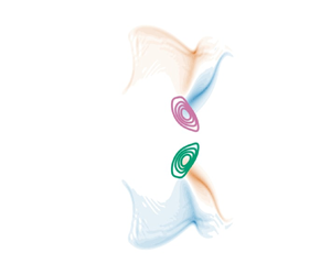
We illustrate the basic workings of the new model by using numerical simulations of simple configurations involving isolated wavepackets and vortex couples. All numerical evidence indicates that wave energy is lost when shocks forms, though we could not prove this statement. A heuristic rule that emerged from these idealized simulations was that, in the long run, the wave field always extracted energy from the mean flow. This raises the question as to whether this ‘greedy waves’ rule holds true for more complicated turbulent scenarios, which would make it relevant to submesoscale ocean energetics, but this was beyond the range of the present paper. We also indicate how to add wave generation and dissipation terms to the model, which allows consideration of a full wavepacket lifecycle and its impact on the mean flow.
The paper is structured as follows. We review elements of GLM theory and derive our reduced model in § 2. Energy conservation for strong solutions is demonstrated in § 3 and the non-standard Riemann theory for suitable weak solutions is developed in § 4. Numerical results for idealized interaction examples are presented in § 5, and in § 6 forcing and dissipation terms are added to the model and illustrated by a wavepacket lifecycle simulation. Concluding remarks are offered in § 7.
2. The GLM theory and model reduction
Here we apply the GLM theory of Andrews & McIntyre (Reference Andrews and McIntyre1978a,Reference Andrews and McIntyreb) to the standard shallow water equations and then use this framework to derive a reduced model for wave–mean interactions. This reduced model describes the joint evolution of two coupled vector fields, one describing the mean flow and one describing the wave field.
2.1. The GLM theory for shallow water equations
We apply exact GLM theory to a shallow water system; fuller details of the GLM theory can be found in the original publications or in Bühler (Reference Bühler2014). The GLM theory distinguishes between mean and actual fluid particle positions, denoted by  $\boldsymbol {x}$ and $\boldsymbol {x}^\xi =\boldsymbol {x}+\boldsymbol {\xi }$, respectively. Here $\boldsymbol {\xi }(\boldsymbol {x},t)$ is the displacement vector, which satisfies $\overline {\boldsymbol {\xi }}=0$, where the overbar denotes any suitable Eulerian averaging operation. To fix ideas, this may be an average over a fast wave time scale, which would be appropriate in oceanography. Formally at least, $\boldsymbol {\xi }$ does not have to be small, i.e. GLM theory is not restricted to small wave amplitudes. The superscript $\xi$ denotes the lifting map, which by definition evaluates any function $\phi (\boldsymbol {x},t)$ at the fluid particle's actual location such that
 \begin{equation} \phi^\xi(\boldsymbol{x},t) = \phi(\boldsymbol{x}^\xi,t). \end{equation}
The Lagrangian average of a function is then defined as the Eulerian average of the lifted function:
 \begin{equation} \overline{\phi}^L(\boldsymbol{x},t) = \overline{\phi^\xi(\boldsymbol{x},t)}. \end{equation}
The Lagrangian disturbance field  $\phi ^\ell = \phi ^\xi - \overline {\phi }^L$ is the difference between the lifted function and its Lagrangian average. A key advantage of GLM theory is the identity
 \begin{equation} \left( \frac{\mathrm{D} \phi}{\mathrm{D} t}\right)^\xi = \overline{\mathrm{D}}^L \phi^\xi , \end{equation}
where
 \begin{equation} \overline{\mathrm{D}}^L =\partial_t + \overline{\boldsymbol{u}}^L\boldsymbol{\cdot}\boldsymbol{\nabla}. \end{equation}
Hence  $\mathrm {D} \phi /\mathrm {D} t = 0$ implies $\overline {\mathrm {D}}^L \overline {\phi }^L = 0$, and note that this uses the Lagrangian-mean velocity $\overline {\boldsymbol {u}}^L$ to advect $\overline {\phi }^L$.
We now apply the GLM formalism to the standard shallow water equations:
 \begin{equation} \frac{\mathrm{D} \boldsymbol{u}}{\mathrm{D} t} + g\boldsymbol{\nabla} h = 0\quad\text{and}\quad \frac{\mathrm{D} h}{\mathrm{D} t} + h \boldsymbol{\nabla} \boldsymbol{\cdot} \boldsymbol{u} = 0, \end{equation}
where  $\boldsymbol {u}$ is the fluid velocity, $h$ is the fluid height and $g$ is gravity. The system possesses a materially conserved PV
 \begin{equation} q = \frac{\boldsymbol{\nabla}\times \boldsymbol{u} }{h} \quad\text{such that}\ \frac{\mathrm{D} q}{\mathrm{D} t} = 0. \end{equation}
In the GLM framework there are analogous equations for the effective mean height field  $\tilde {h}$ and the Lagrangian-mean PV $\overline {q}^L$. The mean height $\tilde {h}$ is defined by
 \begin{equation} \overline{\mathrm{D}}^L \tilde{h} + \tilde{h} \boldsymbol{\nabla} \boldsymbol{\cdot} \overline{\boldsymbol{u}}^L = 0 \end{equation}
and it is related to the displacement field  $\xi$ via
 \begin{equation} \tilde{h} = h^\xi J, \end{equation}
where the Jacobian
 \begin{equation} J =\frac{\partial (x^\xi,y^\xi ) }{\partial (x,y) }. \end{equation}
In general  $\tilde {h}$ need not be equal to either $\overline {h}$ or $\overline {h}^L$, as neither of these necessarily satisfy (2.6). A useful property of $\tilde {h}$ is that the mean volume element $\tilde {h} \,\mathrm {d} x \,\mathrm {d} y$ is advected by $\overline {\boldsymbol {u}}^L$ in the same way as $h \,\mathrm {d} x\, \mathrm {d} y$ is advected by $\boldsymbol {u}$. Just as $J$ lets us swap lifted area elements for mean area elements via $(\mathrm {d} x \,\mathrm {d} y)^\xi = J\, \mathrm {d} x \,\mathrm {d} y$, there is also a tensor ${\mathsf{K}}_{mj}$ that lets us swap lifted surface elements for mean surface elements via $\mathrm {d} S_m^\xi = {\mathsf{K}}_{mj}\,\mathrm {d} S_j$. It is related to $\boldsymbol {\xi }$ via ${\mathsf{K}}_{mj} = \partial J/\partial \xi _{m,j}$, where from now index notation and the Einstein summation convention are used as needed.
Kelvin's circulation theorem for the shallow water equations says that the circulation around a closed material contour is invariant in time, which is well known to underpin the conservation of PV (e.g. Vallis Reference Vallis2017). The GLM analogue of this theorem is derived by expressing this in terms of an integral around the arbitrary lifted closed material contour  $\mathcal {C}^\xi$, and changing coordinates so that this integral is around the mean contour $\mathcal {C}$:
 \begin{equation} \varGamma = \oint_{\mathcal{C}^\xi} u_i \,\mathrm{d} x_i = \oint_\mathcal{C} u_i^\xi\, \mathrm{d} x_i^\xi =\oint_{\mathcal{C}}(u_i^\xi + \xi_{j,i}u_j^\xi)\,\mathrm{d} x_i. \end{equation}
Here we used  $\mathrm {d} x_i^\xi = \mathrm {d} x_i + \xi _{i,j} \, \mathrm {d} x_j$ to get the final equality. Taking the mean of the lifted velocity term will give the Lagrangian-mean velocity but the mean of the second term has not been defined yet; this is the GLM pseudomomentum vector:
 \begin{equation} \boldsymbol{\mathsf{p}} ={-}\overline{\xi_{j,i}u_j^\xi}, \quad \boldsymbol{\mathsf{p}} = \begin{pmatrix} {\mathsf{p}}_1 \\ {\mathsf{p}}_2 \end{pmatrix}. \end{equation}
Taking the mean of (2.8) we obtain
 \begin{equation} \overline{\varGamma} = \oint_{\mathcal{C}} (\overline{\boldsymbol{u}}^L - \boldsymbol{\mathsf{p}})\boldsymbol{\cdot} \mathrm{d} \boldsymbol{x} = \int_{\mathcal{A}} \frac{\boldsymbol{\nabla}\times(\overline{\boldsymbol{u}}^L - {\boldsymbol{\mathsf{p}}})}{\tilde{h}} \tilde{h} \, \mathrm{d} x \,\mathrm{d} y , \end{equation}
where  $\mathcal {A}$ is the surface enclosed by $\mathcal {C}$. Kelvin's circulation theorem tells us this is constant in time and since $\mathcal {C}$ is arbitrary this yields the GLM analogue to (2.5) as
 \begin{equation} \overline{\mathrm{D}}^L \overline{q}^L = 0, \quad \text{with } \ \overline{q}^L = \frac{\boldsymbol{\nabla}\times (\overline{\boldsymbol{u}}^L - \boldsymbol{\mathsf{p}}) }{\tilde{h}}. \end{equation}
Crucially, the velocity  $\overline {{\boldsymbol {u}}}^L-\boldsymbol{\mathsf{p}}$ appearing in the mean circulation is different from the velocity $\overline {{\boldsymbol {u}}}^L$ that advects the mean contour.
The evolution equation for the pseudomomentum is derived by lifting the  $j$th component of the momentum equation in (2.4a,b) and contracting with $-\xi _{j,i}$, which after some manipulations yields
 \begin{equation} \overline{\mathrm{D}}^L {\mathsf{p}}_i + \frac{1}{\tilde{h}} {\mathsf{B}}_{im,m}^{tot} ={-}\overline{u}^L_{k,i} {\mathsf{p}}_k - \frac{\tilde{h}_{,i}}{\tilde{h}} \left( g (\overline{h}^L - \tilde{h}) - \frac{\overline{u_j^\ell u_j^\ell}}{2} \right), \end{equation}
where the pseudomomentum flux tensor
 \begin{equation} {\mathsf{B}}_{im}^{tot} ={-}g\overline{\frac{(h^2)^\xi}{2} \xi_{j,i} {\mathsf{K}}_{jm} } + \frac{\tilde{h}}{2}\delta_{im} \left( \overline{u_j^\ell u_j^\ell} - g (\overline{h}^L - \tilde{h}) \right) . \end{equation}
Hence the  $i$th component of the pseudomomentum is conserved in an integral sense if the mean flow described by $(\overline {{\boldsymbol {u}}}^L,\tilde {h})$ is independent of $x_i$, which is a familiar fact that can be traced back to Noether's theorem (e.g. Salmon Reference Salmon1998). Notably, the pseudomomentum vector field plays an important role in wave–mean interactions whether or not it is conserved.
2.2. Model reduction
The GLM equations above are exact but they are of course far from closed, because they require knowledge of the Lagrangian displacement field  $\boldsymbol {\xi }(\boldsymbol {x},t)$. Moreover, as is well known, the full Lagrangian-mean flow may itself contain a mixture of a slow balanced flow and fast unbalanced waves, which makes extracting the most important interactions a subtle and difficult problem (e.g. Thomas et al. Reference Thomas, Bühler and Smith2018). In the present paper we instead pursue a drastic model reduction that results in a closed dynamical system of PDEs for just $\overline {{\boldsymbol {u}}}^L$ and $\boldsymbol{\mathsf{p}}$. This is achieved in two steps.
First, motivated by the fact that small-Froude-number balanced flows are dominated by their non-divergent component, we ignore any changes in  $\tilde {h}$ and set it equal to a background constant $H$. By (2.6) this implies that $\overline {{\boldsymbol {u}}}^L$ is non-divergent so the first step results in
 \begin{equation} \tilde h = H \quad\text{and}\quad \boldsymbol{\nabla}\boldsymbol{\cdot}\overline{{\boldsymbol{u}}}^L = 0. \end{equation}
This simplifies the pseudomomentum equation (2.12), as the only source term on the right-hand side is now the refraction by the mean flow. The second step is more unusual: we approximate the pseudomomentum flux tensor in (2.12b) by using its ray-tracing expressions for slowly varying wavetrains of non-dispersive waves with intrinsic dispersion relation  $\hat {\omega }=\sqrt {gH}\,|\boldsymbol {k}|$. For such wavetrains the pseudomomentum flux tensor is $H\boldsymbol{\mathsf{p}} \boldsymbol {c}^{g}$, where $\boldsymbol {c}^{g}=\sqrt {gH}{\boldsymbol {k}/|\boldsymbol {k}|}$ is the group velocity. We also have the generic ray-tracing expression, stemming from work done concerning small-amplitude waves (Bretherton & Garrett Reference Bretherton and Garrett1968):
 \begin{equation} \boldsymbol{\mathsf{p}} = \frac{\boldsymbol{k} E}{\hat{\omega}} \quad\Rightarrow\quad \frac{\boldsymbol{\mathsf{p}}}{|\boldsymbol{\mathsf{p}}|} = \frac{\boldsymbol{k}}{|\boldsymbol{k}|}, \end{equation}
where  $E$ is the standard mean wave energy density. Hence we obtain the flux closure
 \begin{equation} \frac{1}{H}{\mathsf{B}}_{im}^{tot} = {\mathsf{p}}_i c^{g}_{m} = \sqrt{gH} \frac{{\mathsf{p}}_i k_m}{|\boldsymbol{k}|} = \sqrt{gH}\frac{{\mathsf{p}}_i {\mathsf{p}}_m}{|\boldsymbol{\mathsf{p}}|}. \end{equation}
This flux is a highly nonlinear function of  $\boldsymbol{\mathsf{p}}$ but still homogeneous of degree one in the components of $\boldsymbol{\mathsf{p}}$, i.e. scaling the pseudomomentum by a non-negative factor will scale the flux by the same factor. As we see in § 4 this greatly affects the self-induced dynamics of the pseudomomentum field. Crucially, (2.15) is the only place where we use an ingredient from ray tracing to formulate our model, no other assumptions about wave amplitudes or length scales being made.
The flow evolution is now entirely determined by  $\overline {{\boldsymbol {u}}}^L(\boldsymbol {x},t)$ and $\boldsymbol{\mathsf{p}}(\boldsymbol {x},t)$ and so the system is closed. We summarize the equations of motions as
 \begin{gather} \boldsymbol{\nabla} \boldsymbol{\cdot} \overline{\boldsymbol{u}}^L = 0, \end{gather}
 \begin{gather}\overline{q}^L = \frac{\boldsymbol{\nabla}\times(\overline{\boldsymbol{u}}^L - \boldsymbol{\mathsf{p}})}{H} \quad\text{and}\quad \overline{\mathrm{D}}^L \overline{q}^L = 0, \end{gather}
 \begin{gather}\overline{\mathrm{D}}^L {\mathsf{p}}_i + \overline{u}_{k,i}^L{\mathsf{p}}_k + \left(\sqrt{gH}\frac{{\mathsf{p}}_i {\mathsf{p}}_m}{|\boldsymbol{\mathsf{p}}|}\right)_{,m} = 0. \end{gather}
Note that due to the nonlinear coupling of  $\overline {{\boldsymbol {u}}}^L$ and $\boldsymbol{\mathsf{p}}$ the amplitude of the wave field does matter for the joint evolution of the system. Indeed, changing the initial size of either of these fields will result in different dynamics. As mentioned in the introduction, our system (2.16) includes ray-tracing dynamics as a subset, albeit with fewer variables and restrictions.
Before moving on, we note that these equations possess an additional integral conservation law that pulls together both  $\overline {q}^L$ and $\boldsymbol{\mathsf{p}}$. The impulse of the flow is defined by
 \begin{equation} {\boldsymbol{\mathsf{I}}} = \int \begin{pmatrix} y \\ -x \end{pmatrix} \overline{q}^L \;H \,\mathrm{d} x \,\mathrm{d} y, \end{equation}
the first rotated moment of  $\overline {q}^L$. The moment can be taken around any centre in $x,y$ and the results below will still hold. For the later numerical simulations on a $2{\rm \pi} \times 2{\rm \pi}$ domain we use ${\rm \pi}$ as the centre for calculating this value.
It can be easily shown from (2.16b) (e.g. Bühler & McIntyre Reference Bühler and McIntyre2005) that this satisfies
 \begin{equation} \frac{\mathrm{d} {\boldsymbol{\mathsf{I}}} }{\mathrm{d} t} = \int \overline{u}_{k,i}^L{\mathsf{p}}_k \, \mathrm{d} x\, \mathrm{d} y. \end{equation}
The right-hand side is the same as the refractive term in the integrated pseudomomentum equation so we can add them together to find
 \begin{equation} \frac{\mathrm{d}}{\mathrm{d} t} ({\boldsymbol{\mathsf{P}}} + {\boldsymbol{\mathsf{I}}} ) = 0, \quad \text{with} \ {\boldsymbol{\mathsf{P}}} = \int \boldsymbol{\mathsf{p}} \; \mathrm{d} x \, \mathrm{d} y. \end{equation}
So we can relate changes in total pseudomomentum to changes in the impulse of  $\overline {q}^L$.
3. Energy conservation
The reduced model (2.16) has an exact energy conservation law, which partitions the total energy into a sum of intrinsic wave energy and of kinetic energy associated with the Lagrangian-mean flow. The appearance of this exact law was unexpected, as retaining energy conservation in reduced models often fails in asymptotic wave–mean interaction theory and typically requires deriving the reduced model using a Hamiltonian framework (e.g. Salmon Reference Salmon1998; Xie & Vanneste Reference Xie and Vanneste2015; Pizzo & Salmon Reference Pizzo and Salmon2021).
There are two ways to derive the energy law. We could either start from the GLM momentum equations for incompressible mean flows or alternatively we could use the vorticity formulation (2.16). The first approach gives some illumination to the local evolution of energy in our domain but it does not come directly from the system of equations we will actually be simulating, so we prefer to use the second method here. See Appendix A for the alternative derivation.
Define a stream function by  $\overline {{\boldsymbol {u}}}^L=(-\psi ^L_y,\psi ^L_x)$ so that
 \begin{equation} \nabla^2 \psi^L = H\overline{q}^L + \boldsymbol{\nabla} \times \boldsymbol{\mathsf{p}} \quad\text{and}\quad \overline{\boldsymbol{u}}^L \boldsymbol{\cdot} \overline{\boldsymbol{u}}^L = |\boldsymbol{\nabla} \psi^L|^2. \end{equation}
With suitable boundary conditions  $\nabla ^2$ is self-adjoint, which leads to the standard formula
 \begin{equation} \frac{1}{2} \frac{\mathrm{d}}{\mathrm{d} t} \int |\boldsymbol{\nabla} \psi^L|^2 \, \mathrm{d} x\, \mathrm{d} y ={-}\frac{1}{2} \frac{\mathrm{d}}{\mathrm{d} t} \int \psi^L \nabla^2 \psi^L \, \mathrm{d} x \,\mathrm{d} y ={-}\int \psi^L \partial_t \nabla^2 \psi^L \, \mathrm{d} x \,\mathrm{d} y. \end{equation}
The curl of the pseudomomentum evolution equation (2.16c) is
 \begin{equation} \overline{\mathrm{D}}^L(\boldsymbol{\nabla}\times\boldsymbol{\mathsf{p}}) + \sqrt{gH} \epsilon_{3jk} \left( \frac{{\mathsf{p}}_k{\mathsf{p}}_m}{|\boldsymbol{\mathsf{p}}|} \right)_{,jm} = 0, \end{equation}
where  $\epsilon _{3jk}$ is the Levi-Civita symbol such that $\boldsymbol {\nabla }\times \boldsymbol{\mathsf{p}} =\epsilon _{3jk}{\mathsf {p}}_{k,j}$. We note in passing that without the group velocity term the pseudomomentum curl is a mean material invariant. Using (2.16b), (3.3) and (3.1a,b) in (3.2) yields
 \begin{equation} -\int \psi^L \partial_t \nabla^2 \psi^L \, \mathrm{d} x \,\mathrm{d} y = \int \psi^L \left(\overline{u}^L_j \nabla^2\psi^L_{,j} + \sqrt{gH} \epsilon_{3jk}\left( \frac{{\mathsf{p}}_k{\mathsf{p}}_m}{|\boldsymbol{\mathsf{p}}|} \right)_{,jm} \right) \, \mathrm{d} x \,\mathrm{d} y. \end{equation}
The first term integrates to zero by  $\boldsymbol {\nabla }\boldsymbol {\cdot }\overline {{\boldsymbol {u}}}^L=0$ and $\overline {{\boldsymbol {u}}}^L\boldsymbol {\cdot }\boldsymbol {\nabla }\psi ^L=0$ whilst the second gives
 \begin{equation} \sqrt{gH} \int \epsilon_{3jk} \psi^L_{,jm} \left( \frac{{\mathsf{p}}_k{\mathsf{p}}_m}{|\boldsymbol{\mathsf{p}}|} \right) \, \mathrm{d} x \,\mathrm{d} y = \sqrt{gH} \int \overline{u}^L_{k,m} \left( \frac{{\mathsf{p}}_k{\mathsf{p}}_m}{|\boldsymbol{\mathsf{p}}|} \right) \, \mathrm{d} x \,\mathrm{d} y \end{equation}
after integrating by parts and using  $\epsilon _{3jk}\psi ^L_{,jm} = \overline {u}^L_{k,m}$. Hence
 \begin{equation} \frac{\mathrm{d}}{\mathrm{d} t} \int \frac{\overline{u}_i^L\overline{u}_i^L}{2} \,\mathrm{d} x\, \mathrm{d} y = \sqrt{gH} \int \overline{u}^L_{k,m} \frac{{\mathsf{p}}_k{\mathsf{p}}_m}{|\boldsymbol{\mathsf{p}}|} \, \mathrm{d} x \,\mathrm{d} y. \end{equation}
Only the symmetric, strain matrix part of  $\boldsymbol {\nabla }\overline {{\boldsymbol {u}}}^L$ enters and the sign of the energy change depends on the alignment of $\boldsymbol{\mathsf{p}}$ with the eigenvectors of that matrix. We turn to the wave energy density
 \begin{equation} E = |\boldsymbol{\mathsf{p}}| \sqrt{gH}. \end{equation}
The equation for  $|\boldsymbol{\mathsf{p}}|$ comes from contracting (2.16c) with $\boldsymbol{\mathsf{p}}/|\boldsymbol{\mathsf{p}}|$ because of the general relation
 \begin{equation} \mathrm{d} |\boldsymbol{\mathsf{p}}| = \frac{\boldsymbol{\mathsf{p}}}{|\boldsymbol{\mathsf{p}}|}\boldsymbol{\cdot}\mathrm{d} \boldsymbol{\mathsf{p}}. \end{equation}
After using the product rule for derivatives this gives
 $$\begin{gather} \overline{{\mathrm{D}}}^L |\boldsymbol{\mathsf{p}}| +\frac{{\mathsf{p}}_i}{|\boldsymbol{\mathsf{p}}|} \overline{u}^L_{k,i} {\mathsf{p}}_k + \left(\sqrt{gH}{\mathsf{p}}_m\right)_{,m} = \sqrt{gH}\frac{{\mathsf{p}}_i{\mathsf{p}}_m}{|\boldsymbol{\mathsf{p}}|}\left(\frac{{\mathsf{p}}_i}{|\boldsymbol{\mathsf{p}}|}\right)_{,m} \nonumber\\ =\frac{\sqrt{gH}}{2}{\mathsf{p}}_m\left(\frac{{\mathsf{p}}_i{\mathsf{p}}_i}{|\boldsymbol{\mathsf{p}}|^2}\right)_{,m}=\frac{\sqrt{gH}}{2}{\mathsf{p}}_m\left(1\right)_{,m}=0. \end{gather}$$
As an alternative way of seeing how the right-hand side vanishes, note that it is a directional derivative of the unit vector  $\boldsymbol{\mathsf{p}}/|\boldsymbol{\mathsf{p}}|$, which is then contracted with $\boldsymbol{\mathsf{p}}$. But any differential of a unit vector is perpendicular to the vector itself so this term is identically zero. Hence the only source term is the refraction term:
 \begin{equation} \frac{\mathrm{d}}{\mathrm{d} t} \int E \, \mathrm{d} x \,\mathrm{d} y = \sqrt{gH} \frac{\mathrm{d}}{\mathrm{d} t} \int |\boldsymbol{\mathsf{p}}| \, \mathrm{d} x \,\mathrm{d} y ={-}\sqrt{gH}\int \frac{{\mathsf{p}}_i{\mathsf{p}}_k}{|\boldsymbol{\mathsf{p}}|} \overline{u}_{k,i}^L \, \mathrm{d} x \,\mathrm{d} y. \end{equation}
Combining with (3.6) gives the total energy conservation law:
 \begin{equation} \frac{\mathrm{d}}{\mathrm{d} t} \int \left(\frac{\overline{u}_i^L\overline{u}_i^L}{2} + E \right) \,\mathrm{d} x \,\mathrm{d} y = \frac{\mathrm{d}}{\mathrm{d} t} \int \left(\frac{\overline{u}_i^L\overline{u}_i^L}{2} + \sqrt{gH} |\boldsymbol{\mathsf{p}}|\right) \,\mathrm{d} x \,\mathrm{d} y = 0. \end{equation}
The energy combines the  $L^2$-norm of $\overline {{\boldsymbol {u}}}^L$ with the $L^1$-norm of $\boldsymbol{\mathsf{p}}$. Notably, this joint conservation law does not depend on the wave amplitude being asymptotically small. It does, however, depend on the flow being smooth, which turns out to be a non-trivial restriction.
4. Weak solutions for the pseudomomentum evolution
The pseudomomentum evolution equation (2.16c) in flux form is
 \begin{equation} \partial_t {\mathsf{p}}_i + \left({\mathsf{p}}_i\overline{u}^L_m+ \sqrt{gH}\frac{{\mathsf{p}}_i {\mathsf{p}}_m}{|\boldsymbol{\mathsf{p}}|}\right)_{,m} + \overline{u}_{k,i}^L{\mathsf{p}}_k = 0. \end{equation}
In the previous sections we assumed that we are dealing with strong solutions of the underlying PDEs and hence the pseudomomentum field is smooth. However, there is a natural tendency for the intrinsic pseudomomentum evolution to develop sharp gradients and indeed to develop discontinuities in finite time. In order to extend our solutions beyond that time we need to develop a suitable notion of weak solutions for  $\boldsymbol{\mathsf{p}}$. We propose to do this based on the integral conservation of both components of $\boldsymbol{\mathsf{p}}= ({\mathsf {p}}_1,{\mathsf {p}}_2)$, which holds in the absence of the refraction term. This leads to a Riemann problem for $\boldsymbol{\mathsf{p}}$ that looks familiar from the generic development of finite volume schemes for hyperbolic equations (e.g. LeVeque Reference LeVeque2002). However, it turns out that our Riemann problem for $\boldsymbol{\mathsf{p}}$ is only weakly hyperbolic, which therefore requires non-standard techniques in order to extract the needed information for use in a finite volume scheme. This is pursued here.
4.1. Riemann problem
For the wave dynamics we use a finite volume algorithm built on Godunov's method, for which the basic step is the solution of one-dimensional Riemann problems at cell interfaces. In (4.1) the highly nonlinear group velocity term is of most interest and its effect on the behaviour of the solution is least obvious. We isolate this term by setting  $\overline {{\boldsymbol {u}}}^L=0$ and $\sqrt {gH}=1$ and considering the one-dimensional Riemann problem
 \begin{equation} \boldsymbol{\mathsf{p}}(x,t=0) = \begin{cases} \boldsymbol{\mathsf{p}}_l, & x<0 \\ \boldsymbol{\mathsf{p}}_r, & x>0 \end{cases} \quad \text{with} \ \partial_t \boldsymbol{\mathsf{p}} + \partial_x \left(\boldsymbol{\mathsf{p}}\frac{{\mathsf{p}}_1}{|\boldsymbol{\mathsf{p}}|}\right) = 0. \end{equation}
The constant vectors  $\boldsymbol{\mathsf{p}}_l$ and $\boldsymbol{\mathsf{p}}_r$ are the left and right states of the Riemann problem. This reduces to a textbook problem if ${\mathsf {p}}_2=0$ on both sides, as then ${\mathsf {p}}_1$ satisfies
 \begin{equation} \partial_t{\mathsf{p}}_1+\partial_x|{\mathsf{p}}_1| = 0. \end{equation}
If  ${\mathsf {p}}_{1l}>0$ and ${\mathsf {p}}_{1r}<0$ then the standard Rankine–Hugoniot procedure delivers the well-known solution of a shock moving with speed
 \begin{equation} v=\frac{|{\mathsf{p}}_{1l}|-|{\mathsf{p}}_{1r}|}{|{\mathsf{p}}_{1l}|+|{\mathsf{p}}_{1r}|}. \end{equation}
However, this is of little help for the two-component problem, as we shall see. Written in matrix form (4.2) becomes
 \begin{equation} \partial_t \begin{pmatrix} {\mathsf{p}}_1 \\ {\mathsf{p}}_2 \end{pmatrix} + \partial_x\begin{pmatrix} {\mathsf{p}}_1c \\ {\mathsf{p}}_2c \end{pmatrix}= 0 \quad\Rightarrow\quad \partial_t \begin{pmatrix} {\mathsf{p}}_1 \\ {\mathsf{p}}_2 \end{pmatrix} + \begin{pmatrix} c + cs^2 & -c^2s \\ s - sc^2 & c^3 \end{pmatrix} \partial_x \begin{pmatrix} {\mathsf{p}}_1 \\ {\mathsf{p}}_2 \end{pmatrix} = 0, \end{equation}
where  $c={\mathsf {p}}_1/|\boldsymbol{\mathsf{p}}|$ and $s={\mathsf {p}}_2/|\boldsymbol{\mathsf{p}}|$ denote the cosine and sine of the angle between $\boldsymbol{\mathsf{p}}$ and the $x$ axis. The matrix is known as the flux Jacobian matrix and the eigenvalues of the matrix are the characteristic speeds with which information travels. The matrix is called strictly hyperbolic if there are two distinct real eigenvalues and strongly hyperbolic if there is a single real eigenvalue but two distinct eigenvectors. However, in the present case there is only one eigenvalue–eigenvector pair, namely
 \begin{equation} \lambda = c \quad\text{and}\quad\boldsymbol{r}=\begin{pmatrix} c \\ s \end{pmatrix}, \end{equation}
and then the matrix is called weakly hyperbolic. So we are dealing with a weakly hyperbolic system in (4.5).
Before exploring this issue further we note that for the purpose of numerical integration with a finite volume scheme we need to know the flux vector only at the interface  $x=0$ for $t>0$, i.e. it is not necessary to know the solution for all values of the Godunov similarity variable $x/t$, but only for $x/t=0$. In most cases this does not require working out the full solution. For example, let $(c_l,c_r)$ be the left and right values of the characteristic speed. If there is a shock moving with speed $v$ then the Lax stability criterion requires that $c_l\geq v\geq c_r$. Hence if both $c_l$ and $c_r$ are positive then so is $v$, which implies that the interface state at $x/t=0$ is the left state ${\mathsf {p}}_l$, and vice versa for the opposite sign. Also, if $c_l<0$ and $c_r>0$ then there is a smooth expansion fan centred at the interface such that $c(x,t)=x/t$ and therefore the flux $\boldsymbol{\mathsf{p}} c$ at $x/t=0$ is the zero vector. This leaves $c_l>0$ and $c_r<0$ as the only case in which the flux at $x/t=0$ is not known a priori. It would be tempting to close the problem using an ad hoc rule such that the sign of $v$ is equal to the sign of the speed average $(c_l+c_r)/2$, say, but it turns out that this would give the wrong answer.
When considering this case the crucial problem is that there is only one shock wave in this two-variable system and hence the usual Rankine–Hugoniot construction fails to produce a shock speed  $v$ that can satisfy both conservation laws for all choices of left and right state. It is therefore not clear how to proceed, but inspiration can be found from a linear example that can be solved exactly.
4.2. The  $\delta$-shock solution

Consider the Riemann problem for the following linear weakly hyperbolic system for  $\boldsymbol {u}=(u,v)$:
 \begin{equation} \boldsymbol{u}(x,t=0) = \begin{cases} \boldsymbol{u}_{l}, & x<0 \\ \boldsymbol{u}_{r}, & x>0 \end{cases} \quad \text{with}\ \partial_t \begin{pmatrix} u \\ v \end{pmatrix} + \begin{pmatrix} 1 & 1 \\ 0 & 1 \end{pmatrix} \partial_x\begin{pmatrix} u \\ v \end{pmatrix} = 0. \end{equation}
This has a single eigenvalue  $\lambda = 1$ and eigenvector $\boldsymbol {r} = (1,0)^{\rm T}$. This tridiagonal example is sufficient because any other linear system can be brought into this form by premultiplying with the left eigenvectors of the system. By inspection, the exact solution to the general initial-value problem is given by $v(x,t)=v(x-t,0)$ and
 \begin{equation} u(x,t) = u(x-t,0) - tv_{x}(x-t,0). \end{equation}
In the Riemann problem there is a discontinuity in the initial condition and hence  $v_x(x,0)$ has a $\delta$-function at $x=0$. Hence the solution to (4.7) is
 \begin{equation} \boldsymbol{u} = \left\{\begin{matrix} \boldsymbol{u}_l & x< t\\ \ t\delta(x-t) \begin{pmatrix}v_l-v_r \\ 0 \end{pmatrix} & x=t\\ \boldsymbol{u}_r & x>t.\\ \end{matrix}\right. \end{equation}
It is now apparent how a weakly hyperbolic system achieves conservation of two variables with just one shock wave: for almost all initial conditions there is a growing  $\delta$-function contribution located on the shock wave itself. Consideration of the usual flux balance together with this $\delta$-function contribution then achieves the integral conservation of $\boldsymbol {u}$.
With this linear example in mind we postulate that the solution to the nonlinear (4.5) likewise contains a growing  $\delta$-function on the shock wave. This is consistent with the Godunov similarity variable $x/t$ because $t\delta (x-vt)=\delta (x/t-v)$ for $t>0$. So we write
 \begin{equation} \boldsymbol{\mathsf{p}} = \boldsymbol{\mathsf{p}}_l + (\boldsymbol{\mathsf{p}}_r-\boldsymbol{\mathsf{p}}_l)H(x-vt) + \begin{pmatrix} a \\ b \end{pmatrix}t\delta(x-vt), \end{equation}
where  $v$ is the shock speed, $H$ is the Heaviside function and $(a,b)$ are constants. In contrast with the linear example both $v$ and $(a,b)$ are functions of the initial state that are yet to be determined. (In practice the $\delta$-function will not have infinite amplitude in a numerical simulation, but our Godunov-based scheme results in sharp spikes in the solution, as others have seen in related numerical investigations (e.g. Garg & Gowda Reference Garg and Gowda2022).)
We integrate (4.2) using (4.10) over a small interval containing the shock and enforce conservation of  $\boldsymbol{\mathsf{p}}$ as we would to find the standard Rankine–Hugoniot condition, but instead we find the two generalized Rankine–Hugoniot conditions
 \begin{equation} v(\boldsymbol{\mathsf{p}}_r-\boldsymbol{\mathsf{p}}_l) = c_r \boldsymbol{\mathsf{p}}_r - c_l\boldsymbol{\mathsf{p}}_l + \begin{pmatrix} a \\ b \end{pmatrix}. \end{equation}
A third equation to complete the system is found by considering the homogeneous expression for the characteristic speed  $c={\mathsf {p}}_1/\sqrt {{\mathsf {p}}_1^2+{\mathsf {p}}_2^2}$ near the shock. From (4.10) the dominant parts of ${\mathsf {p}}_1$ and ${\mathsf {p}}_2$ are $at\delta (x-vt)$ and $bt\delta (x-vt)$, respectively, because when integrating over a small interval containing the shock the other terms are insignificant. The same result can be had by considering a regularized $\delta$-function that has been broadened over an arbitrarily small interval containing $x=vt$. Consistency between the shock speed $v$ and the characteristic speed formula then requires using the coefficients of the $\delta$-function in the expression for the characteristic speed $c$, which yields
 \begin{equation} v = \frac{a}{\sqrt{a^2+b^2}}. \end{equation}
This third equation completes the solution to the Riemann problem and therefore the construction of the relevant weak solution for our system.
The fact that weakly hyperbolic systems may feature  $\delta$-function shocks is known in the wider physics literature; for example, this arises in the study of pressureless gas dynamics as a model for dust aggregation (Leveque Reference Leveque2004). We also became aware recently that our heuristic construction for solving (4.2) can be made mathematically rigorous and provably leads to a unique weak solution, at least when ${\mathsf {p}}_{2l}$ and ${\mathsf {p}}_{2r}$ have the same sign (Yang Reference Yang1999). (Our problem is (6.14) in that paper, with our $(a,b)$ corresponding to $(w_0U_\delta, w_0)$ there.)
Finding the full solution of (4.11) and (4.12) involves a quartic equation, but fortunately we can easily find the sign of  $v$ analytically, which is all that is needed for a finite volume discretization. Substituting (4.12) into (4.11) and rearranging the first component gives
 \begin{equation} v\left(\sqrt{a^2+b^2}+{\mathsf{p}}_{1l} - {\mathsf{p}}_{1r}\right) = c_l {\mathsf{p}}_{1l} - c_r {\mathsf{p}}_{1r}. \end{equation}
Since  $({\mathsf {p}}_{1r},{\mathsf {p}}_{1l})$ have the same signs as $(c_r,c_l)$ and because in the case of interest $c_l>0$ and $c_r<0$, we know that the parenthesis is positive. Therefore the sign of $v$ is equal to the sign of the right-hand side, i.e.
 \begin{equation} \operatorname{sgn}{v} = \operatorname{sgn}{(c_l {\mathsf{p}}_{1l} - c_r {\mathsf{p}}_{1r})}. \end{equation}
Hence if  $c_l {\mathsf {p}}_{1l} > c_r {\mathsf {p}}_{1r}$ then the interface state is $\boldsymbol{\mathsf{p}}_l$ and vice versa for the opposite case. In summary, the state possessing the larger ${\mathsf {p}}_1$ flux determines the overall flux of $\boldsymbol{\mathsf{p}}$, which would have been a difficult rule to guess.
4.3. Wave energy loss in weak solutions
It is easy to think of examples where the weak solution developed above conserves  $\boldsymbol{\mathsf{p}}$ but loses $|\boldsymbol{\mathsf{p}}|$ and hence loses wave energy. The simplest one-dimensional example consists of two counter-propagating wavepackets moving towards each other along the $x$ axis such that ${\mathsf {p}}_1$ changes sign and ${\mathsf {p}}_2=0$ throughout. After colliding head-on there will only be a single wavepacket remaining, with net pseudomomentum equal to the sum of the pseudomomentum of the original two wavepackets. It is clear that in this case $|\boldsymbol{\mathsf{p}}|$ is not conserved; indeed in the limiting case of equal-and-opposite wavepackets the net outcome of the collision is the complete disappearance of the waves and therefore all wave energy has been lost.
We are not claiming that this wave energy loss is a realistic or even desirable feature of our model, which is really aimed towards two-dimensional interactions, where head-on collisions are much rarer and less important than wavepacket deformation, focusing and refraction effects, as is illustrated later. Still, it would be a desirable feature for the weak solution if the wave energy change were non-positive, i.e. if the weak solutions never generated extra wave energy but only ever destroyed it. This would make the wave energy in our model analogous to the entropy in gas dynamics, or to the energy in shallow water flow, which can only change in a sign-definite way when shocks form (e.g. Dafermos Reference Dafermos2016).
Unfortunately, although all numerical evidence points to its validity, we have not been able to prove this statement rigorously, not even in a one-dimensional setting. This is therefore an open question, and we briefly outline here how far we have been able to pursue it. Our approach has been to start with the conservation law for  $|\boldsymbol{\mathsf{p}}|$ in (3.9), which in a one-dimensional setting with $\overline {{\boldsymbol {u}}}^L=0$ and $\sqrt {gH}=1$ is
 \begin{equation} \partial_t |\boldsymbol{\mathsf{p}}| + \partial_x {\mathsf{p}}_{1} = 0. \end{equation}
Integrating this scalar conservation law over a small interval  $x\in [x_0,x_1]$ containing the shock and enforcing conservation of $|\boldsymbol{\mathsf{p}}|$ yields
 \begin{equation} \frac{\mathrm{d}}{\mathrm{d} t} \int_{x_0}^{x_1} |\boldsymbol{\mathsf{p}}|\,\mathrm{d} x = {\mathsf{p}}_{1l}-{\mathsf{p}}_{1r}. \end{equation}
So, if the change in  $|\boldsymbol{\mathsf{p}}|$ in the interval is just equal to the right-hand side of (4.16) then wave energy is conserved. For our weak solution to not increase the system's wave energy we therefore need that this integral calculated with (4.10) is less than or equal to ${\mathsf {p}}_{1l}-{\mathsf {p}}_{1r}$, which is the statement we would like to prove. Calculating $|\boldsymbol{\mathsf{p}}|$ from (4.10) we find
 \begin{gather} |\boldsymbol{\mathsf{p}}| = \sqrt{{\mathsf{p}}_{1l}^2 +{\mathsf{p}}_{2l}^2 } + \left(\sqrt{{\mathsf{p}}_{1r}^2 + {\mathsf{p}}_{2r}^2} - \sqrt{{\mathsf{p}}_{1l}^2 +{\mathsf{p}}_{2l}^2 } \right) H(x-vt) + t\sqrt{a^2+b^2}\delta(x-vt) \end{gather}
 \begin{gather}\quad\Rightarrow\quad \frac{\mathrm{d}}{\mathrm{d} t}\int_{x_0}^{x_1} |\boldsymbol{\mathsf{p}}| \,\mathrm{d} x = v\left(\sqrt{{\mathsf{p}}_{1l}^2 +{\mathsf{p}}_{2l}^2 } - \sqrt{{\mathsf{p}}_{1r}^2 + {\mathsf{p}}_{2r}^2}\right) + \sqrt{a^2+b^2}. \end{gather}
So the statement to prove is that the validity of (4.12) and (4.11) implies
 \begin{equation} v\left(\sqrt{{\mathsf{p}}_{1l}^2 +{\mathsf{p}}_{2l}^2 } - \sqrt{{\mathsf{p}}_{1r}^2 + {\mathsf{p}}_{2r}^2}\right) + \sqrt{a^2+b^2} \leq {\mathsf{p}}_{1l}-{\mathsf{p}}_{1r} \end{equation}
for all choices of  $(\boldsymbol{\mathsf{p}}_l,\boldsymbol{\mathsf{p}}_r)$ with ${\mathsf {p}}_{1l}>0$ and ${\mathsf {p}}_{1r}<0$. We have only been able to verify this in the trivial case where ${\mathsf {p}}_2=0$ throughout. In that case $a=b=0$, so there is no $\delta$-shock, and the shock speed is given by (4.4), which immediately satisfies (4.19).
In the general case with non-zero  ${\mathsf {p}}_2$ the validity of (4.19) can be checked numerically using a root-finding algorithm such as Newton's method to solve the underlying quartic equations. We have tested this for $({\mathsf {p}}_{1l},{\mathsf {p}}_{2l},{\mathsf {p}}_{1r},{\mathsf {p}}_{2r})\in [-3,3]^4$ with intervals of $1/8$ and did not find a counterexample, though this is of course not a proof.
5. Numerical results
We simulate (2.16) on a two-dimensional torus by using Strang operator splitting to alternate between the two flux and refraction equations
 \begin{equation} \partial_t \begin{pmatrix} \boldsymbol{\mathsf{p}} \\ \overline{q}^L \end{pmatrix} + \partial_x \begin{pmatrix} (\sqrt{gH}c + \overline{u}^L) \boldsymbol{\mathsf{p}} \\ \overline{u}^L \overline{q}^L \end{pmatrix} + \partial_y \begin{pmatrix} (\sqrt{gH}s + \overline{v}^L) \boldsymbol{\mathsf{p}} \\ \overline{v}^L \overline{q}^L \end{pmatrix} = 0 \end{equation}
and
 \begin{equation} \partial_t \boldsymbol{\mathsf{p}} + (\boldsymbol{\nabla} \overline{\boldsymbol{u}}^L ) \boldsymbol{\cdot} \boldsymbol{\mathsf{p}} = 0, \end{equation}
where  $\boldsymbol{\mathsf{p}}$ contracts with $\overline {\boldsymbol {u}}^L$ not $\boldsymbol {\nabla }$. The numerical scheme for the two-dimensional flux terms in (5.1a) is further split into parts for the $x$ and $y$ flux components so that we can use the results for the one-dimensional Riemann problem. For strong solutions this algorithm will be second-order accurate overall provided the number of time steps is even and the algorithms for both equations are separately second-order accurate.
We use Godunov's method with linearly reconstructed states and the monotonized central slope limiter, as part of a second-order Runge–Kutta scheme, Heun's method, for each of these. The scheme for the refractive part is also Heun's method, where we calculate the gradients of  $\overline {\boldsymbol {u}}^L$ spectrally (and apply a Gaussian filter of standard deviation $\Delta x$ in case of shocks having formed, where $\Delta x$ is the spatial step size). The mean flow velocity $\overline {\boldsymbol {u}}^L$ is updated according to (2.16b) whenever $\boldsymbol{\mathsf{p}}$ and $\overline {q}^L$ are updated.
The time step is determined from the sum of maximum initial mean flow speed and the group velocity according to the Courant–Friedrichs–Lewy (CFL) condition, with CFL number 0.025, and the domain contains  $N=1024$ grid points for a spacing of $\Delta x = 2{\rm \pi} /N$ in both directions. This very small CFL number is picked due to the refraction matrix $\boldsymbol {\nabla } \overline {\boldsymbol {u}}^L$ having a positive eigenvalue, so we do this to minimize as much as possible the amplification of errors. Finally, we set $g=H=1$ so that $c^{g} = 1$.
5.1. Isolated wavepacket
The first results we show are for an isolated wavepacket where the initial condition has  $\overline {q}^L = 0$. Since the Lagrangian-mean PV is initially zero it remains zero and so the induced mean flow is found from $\boldsymbol {\nabla }\times \overline {{\boldsymbol {u}}}^L=\boldsymbol {\nabla }\times \boldsymbol{\mathsf{p}}$ and $\boldsymbol {\nabla }\boldsymbol {\cdot }\overline {{\boldsymbol {u}}}^L=0$. The initial condition is
 \begin{equation} {\mathsf{p}}_1 = A\exp({-(100(x-({\rm \pi}-0.5))^2 + 25(y-{\rm \pi})^2)}) \quad\text{and}\quad {\mathsf{p}}_2=0. \end{equation}
The corresponding  $\boldsymbol {\nabla }\times \boldsymbol{\mathsf{p}}$ is a dipole flanking the wavepacket and hence $\overline {{\boldsymbol {u}}}^L$ is a standard vortex couple flow. The evolution of $\boldsymbol{\mathsf{p}}$ is therefore a combination of propagation by the group velocity plus advection and refraction by the mean-flow vortex couple. The numbers 100 and 25 have been chosen large enough so that periodic boundary effects are negligible, while still having a wavepacket that is resolved by the grid spacing, and $A$ is picked so that the maximum initial velocity induced by $\boldsymbol{\mathsf{p}}$ alone,
 \begin{equation} U_{\boldsymbol{\mathsf{p}}} = \max{|\overline{\boldsymbol{u}}^L|_{t=0}}| \quad \text{with} \ \overline{q}^L = 0, \end{equation}
is given the values 0.05, 0.2 and 0.5. We pick three scalings of the pseudomomentum field to investigate how the evolution changes due to the pseudomomentum flux, as mentioned before. The third of these has a maximum velocity of 0.5, which is towards the larger end of what we might call small (considering the small-Froude-number assumption we used in our derivation); however, it is included here and in later figures in order to exaggerate the qualitative effects we see. The corresponding values of  $A$ are 0.152, 0.608 and 1.521. The initial ${\mathsf {p}}_1$ and its subsequent evolution are illustrated in figure 1.

Figure 1. Simulations of an isolated wavepacket, showing solutions at  $t=0,1$ for $U_{\boldsymbol{\mathsf{p}}} =$ (a–d) 0.05, (e–h) 0.2 and (i–l) 0.5. (a,e,i) Component ${\mathsf {p}}_1$, (b,f,j) ${\mathsf {p}}_2$, (c,g,k) $\boldsymbol {\nabla }\times \boldsymbol{\mathsf{p}}$ and (d,h,l) the energy over time. In each experiment, the plots for ${\mathsf {p}}_1$ and ${\mathsf {p}}_2$ share the same colourbar. Only a central region of the domain is shown.
If we were in the absence of a mean-flow velocity, there would be no refractive effects so  ${\mathsf {p}}_2$ remains zero and this initial condition would translate to the right with constant speed $c^{g}=1$. However, the inclusion of a mean flow changes this: the mean-flow vortices give an additional mean-flow velocity to the right in between the vortices, which pushes the initially straight ${\mathsf {p}}_1$ into a bow shape. As $U_{\boldsymbol{\mathsf{p}}}$ increases, the bow shape that develops becomes larger, and $\boldsymbol {\nabla }\times \boldsymbol{\mathsf{p}}$ also becomes more smeared out. This is where we can also observe the effect of the group velocity term as, in its absence, $\boldsymbol {\nabla }\times \boldsymbol{\mathsf{p}}$ would be materially advected, from (3.3).
Refraction also generates  ${\mathsf {p}}_2$, which in fact leads to an increase in wave energy. This is due to the conservation of ${\boldsymbol{\mathsf{P}}} + {\boldsymbol{\mathsf{I}}}$, (2.19), since $\overline {q}^L=0$ so ${\boldsymbol{\mathsf{I}}}=0$ too. Specifically this implies that even with the refractive effects present, the integrals of ${\mathsf {p}}_1$ and ${\mathsf {p}}_2$ are both conserved, so $|\boldsymbol{\mathsf{p}}|$ must increase with the generation of ${\mathsf {p}}_2$ (at least for some initial period of time). Indeed, the conservation of ${\mathsf {p}}_2$ is satisfied for $t>0$ as for each region where it becomes positive there is another region where it is negative so that the integral remains zero, which can be seen in figure 1(b,f,j). Concomitant with an increase in wave energy is a decrease in mean-flow energy, which is also seen from figure 1(d,h,l).
This increase in wave energy is not something that happens for all initial conditions for all time. For example, there is a symmetry in the equations given by  $(\boldsymbol{\mathsf{p}},\overline {\boldsymbol {u}}^L,t) \rightarrow (-\boldsymbol{\mathsf{p}},-\overline {\boldsymbol {u}}^L, -t)$, so given a strong solution to the equation at some $t>0$ we can reverse time and therefore reverse the direction of the energy exchange.
Nevertheless, we found this to be quite a general heuristic rule: in the long run the wave field tends to gain energy from the mean flow. An illustration of this is provided by the next example.
5.2. Focusing wavepacket
We now consider a focusing wavepacket, where the initial condition has  ${\mathsf {p}}_2\neq 0$ such that the group velocity points towards the centreline $y={\rm \pi}$ from above and below. This implies that the strong solution breaks down in finite time and therefore our weak solution strategy is essential to proceed past that breakdown time. Notably, a standard ray-tracing scheme would also fail in this case, and predict infinite amplitudes during the focusing. However, as we shall see, our weak solution proceeds through the focusing episode in a natural fashion and subsequently we again recover a strong solution.
In particular, the initial condition for  ${\mathsf {p}}_1$ is still specified by (5.2a,b), but
 \begin{equation} {\mathsf{p}}_2 ={-}2.5A (y-{\rm \pi})\exp({-(100(x-({\rm \pi}-0.5))^2 + 25(y-{\rm \pi})^2)}). \end{equation}
The constant  $A$ is again chosen to give the initial velocity field the same maximum values $U_{\boldsymbol{\mathsf{p}}}$ of 0.05, 0.2 and 0.5. In particular the values of $A$ are 0.142, 0.569 and 1.421. In figure 2 we show these experiments, with the same increasing values of $U_{\boldsymbol{\mathsf{p}}}$ for each row. In each case, ${\mathsf {p}}_2$ starts with a negative region above a positive region, then at $t=1$ they have swapped and changed shape. The graphs of the wave and mean-flow energies show an initial decrease in wave energy, before the same wave energy saturation happens as in figure 1. The distributions of $\boldsymbol {\nabla }\times \boldsymbol{\mathsf{p}}$ at $t=1$ vary widely, especially around $y={\rm \pi}$, showing that the shocks mentioned in § 4.1 have formed, which is different from the previous set of experiments. However, this has not led to a significant decrease in the total energy, which has stayed roughly constant. Crucially, the wave energy decreases during the early focusing episode, but subsequently it increases again, and in the long run there is again a net gain of wave energy at the expense of the mean-flow energy.

Figure 2. Simulations of an initially focusing wavepacket, showing solutions at  $t=0,1$. The rows and columns are ordered the same as figure 1, and the domain being plotted is also the same in each panel.
Before moving on to a more complicated example, we show in figure 3 plots of the energy conversion integrand,  $\overline {u}^L_{k,m} {\mathsf {p}}_k{\mathsf {p}}_m/|\boldsymbol{\mathsf{p}}|$ from (3.6), for the experiments with $U_{\boldsymbol{\mathsf{p}}}=0.5$ in the previous two figures. In figure 3(a), we see that the energy which is dominantly being converted to wave energy at the front (right side) of the wavepacket is being exactly balanced by a region of mean flow energy transfer to the rear of the wavepacket. This is because of the symmetric initial condition that was chosen. In figure 3(b), the $t=1$ evolution for the initial condition in figure 3(a), there is an imbalance where most of the energy is being accumulated by the waves. In particular, this is happening at the front of the wavepacket, and the rate of energy transfer into mean-flow energy behind the wavepacket is significantly diminished.

Figure 3. Plots of the energy conversion integrand from (3.6), for the simulations in figures 1 and 2, at times  $t=0,1$. Positive values denote energy being transferred from the waves to the mean flow, and vice versa. The colourbar axis for (d) has been decreased by a factor of 10 in order to see more details in the wavepacket as a whole, and not just the large negative values at $y={\rm \pi}$.
In the second experiment (figure 3c,d), where the wavepacket is initially focusing, there is a region of stronger wave-to-mean-flow energy transfer at  $t=0$ corresponding to the initial decrease in wave energy in figure 2(l). After the shock has formed this is no longer present, and rather we see a similar bow-shaped region of wave energy accumulation as in figure 3(a).
5.3. Wavepacket and mean-flow vortices
Finally, we look at the interaction of a wavepacket with a mean flow coming from a non-zero  $\overline {q}^L$. In particular we consider the experiment where we have a vortex couple in $\overline {q}^L$,
 \begin{equation} \overline{q}^L ={\pm} 50B(y-{\rm \pi})\exp({-(100(x-({\rm \pi}+0.5))^2 + 25(y-{\rm \pi})^2)}), \end{equation}
as well as the wavepacket defined in (5.2a,b), but with a wider footprint in the  $x$ direction, ${\mathsf {p}}_1 \propto \exp ({-5(x-({\rm \pi} -0.5))^2})$ (and ${\mathsf {p}}_2=0$) in order to exaggerate the qualitative effects of these interactions. In this configuration the group velocity on its own will move the wavepacket to the right whilst the vortex couple in $\overline {q}^L$ on its own would move to the right or the left depending on the sign choice in (5.5). This is similar to the wave–vortex structure of the main examples in Bühler & McIntyre (Reference Bühler and McIntyre2005), but the ray-tracing analysis in that paper did not provide a complete quantitative description of energy exchanges during the interactions.
The constant  $B$ is chosen in the same way as the constant $A$ for the wavepacket, but scaling according to the velocity induced by $\overline {q}^L$ alone:
 \begin{equation} U_{\overline{q}^L} = \max{|\overline{\boldsymbol{u}}^L|_{t=0}}| \quad \text{with} \ \boldsymbol{\mathsf{p}} = 0. \end{equation}
We choose  $A$ and $B$ such that $U_{\boldsymbol{\mathsf{p}}} = U_{\overline {q}^L} = 0.5$ ( $A = 0.731$, $B = 1.504$) and perform two experiments where the sign of $\overline {q}^L$ is flipped between them. With these initial conditions, the wavepacket and vortex pair move towards or away from each other (see figure 4). These high values of $U_{\boldsymbol{\mathsf{p}}}$ and $U_{\overline {q}^L}$ have been chosen again to exaggerate qualitative effects, and to display more succinctly the results of our simulations, rather than choosing three different values as in figures 1 and 2. The plots of ${\mathsf {P}}_1$ and ${\mathsf {I}}_1$ are also shown this time due to there being non-zero $\overline {q}^L$. Due to the symmetry of the initial conditions, the net ${\mathsf {P}}_2$ and ${\mathsf {I}}_2$ are identically zero. As in the previous two examples, the wavepacket expands for an initial period of time, which is shown by the regions of positive (negative) $\boldsymbol {\nabla }\times \boldsymbol{\mathsf{p}}$ above (below) $y={\rm \pi}$ at $t=0.5$ in both cases, but the presence of the oncoming vortex pair (figure 4a–d) causes different behaviours in the centre of the domain. There is generation of positive $\boldsymbol {\nabla }\times \boldsymbol{\mathsf{p}}$ above negative $\boldsymbol {\nabla }\times \boldsymbol{\mathsf{p}}$ in front of the wavepacket either side of $y={\rm \pi}$, which gives a mean-flow velocity to the right. This comes from the group velocity flux term as, without this, $\boldsymbol {\nabla }\times \boldsymbol{\mathsf{p}}$ is materially conserved, as already pointed out. The fact that this extends to only a thin region in the $y$ direction points to the generation of a ${\mathsf {p}}_2$ (not shown) which causes focusing of the wavepacket, as in figure 2. As such, shocks form in $\boldsymbol{\mathsf{p}}$ and the distribution of $\boldsymbol {\nabla }\times \boldsymbol{\mathsf{p}}$ is very complicated at $t=1,1.5$. The evolution between times $t=0.5$ and 1.5 shows again a defocusing expansion of the wavepacket after moving through the vortex dipole. With the shocks that form comes a small decrease in the total energy, which is lost from the wave energy. This aside, figure 4(i) shows that the wave energy increases substantially over the total time considered, and we see again that in the long run wave energy grows at the expense of mean-flow energy.

Figure 4. Simulations of wavepackets interacting with oncoming and retreating vortex couples (the sign of  $\overline {q}^L$ is flipped). In both, $U_{\boldsymbol{\mathsf{p}}} = U_{\overline {q}^L} = 0.5$. The plotted fields in (a–h) are $\boldsymbol {\nabla } \times \boldsymbol{\mathsf{p}}$ and $\overline {q}^L$, at $t=0,0.5,1,1.5$. Only a central region of the domain is shown. (i–l) The energies and momentum-like terms over time.
For the second case where the vortex pair is retreating (figure 4e–h), we see the same wavepacket expansion up to  $t=0.5$, but now we have generation of negative $\boldsymbol {\nabla }\times \boldsymbol{\mathsf{p}}$ above positive $\boldsymbol {\nabla }\times \boldsymbol{\mathsf{p}}$ at the front of the wavepacket, which causes a weak flow in the negative $x$ direction along $y={\rm \pi}$. Most interestingly, this pattern alongside the rest of the $\boldsymbol {\nabla }\times \boldsymbol{\mathsf{p}}$ distribution gives velocities pointing diagonally up (down) and rightwards above (below) $y={\rm \pi}$. This is a pattern which we see getting stronger over time as the rest of the wavepacket comes to interact with $\overline {q}^L$.
The importance of this is that it causes  $\overline {q}^L$ to be moved away from the centreline. In the absence of the group velocity flux term we would already expect this, as we would then have a pair of vortices in $\boldsymbol {\nabla }\times \boldsymbol{\mathsf{p}}$ approaching a pair of vortices in $\overline {q}^L$, all being advected by the mean velocity. However, due to the the spreading out of $\boldsymbol {\nabla }\times \boldsymbol{\mathsf{p}}$ it was not obvious this would still happen as $\boldsymbol {\nabla }\times \boldsymbol{\mathsf{p}}$ weakens. Figure 4(h) confirms the separating of the vortex pair because ${\mathsf {I}}_1$ is increasing for the whole evolution. A similar observation might be made for the first examples to say that the $\overline {q}^L$ vortices get closer, but the change in ${\mathsf {P}}_1$ and ${\mathsf {I}}_1$ is very small there, and is not monotonic (so this only happens up until approximately $t=0.7$ before reverting). Once again, the net energy exchange converts mean-flow energy into wave energy in both cases, and therefore in all the experiments we have considered here.
6. Forcing and dissipation
Forcing terms can be added to the reduced wave–vortex model (2.16) to model important physical processes such as wave generation or dissipation. For example, it is well recognized that dissipating waves give rise to an effective mean force whose curl acts on the mean PV field (e.g. McIntyre & Norton Reference McIntyre and Norton1990). In the simplest scenarios that effective mean force is approximately equal and opposite to the local dissipation density of pseudomomentum, which is the pseudomomentum rule that underpins wave drag parametrizations in atmospheric models. Conversely, wave forcing per se affects the pseudomomentum but not the PV, at least not directly. Hence wave generation and wave dissipation are represented quite differently in our reduced model.
6.1. Effective mean forces in GLM theory
A general discussion of forcing terms in GLM theory has been given in Bühler (Reference Bühler2000) and Bühler & McIntyre (Reference Bühler and McIntyre2005), so we just summarize the outcome. If an arbitrary force per unit mass  $\boldsymbol {F}$ is added to the momentum equations then (2.16b) and (2.16c) become
 \begin{equation} \overline{\mathrm{D}}^L \overline{q}^L = \frac{\boldsymbol{\nabla}\times \tilde{\boldsymbol{F}}}{H} \end{equation}
and
 \begin{equation} \overline{\mathrm{D}}^L {\mathsf{p}}_i + \overline{u}_{k,i}^L{\mathsf{p}}_k + \left(\sqrt{gH}\frac{{\mathsf{p}}_i {\mathsf{p}}_m}{|\boldsymbol{\mathsf{p}}|}\right)_{,m} = \mathcal{F}_i ,\end{equation}
where
 \begin{equation} \overline{{\boldsymbol{F}}}^L=\overline{\boldsymbol{F}^\xi},\quad \mathcal{F}_i ={-}\overline{\xi_{j,i}F^\xi_j} \quad \text{and}\quad \tilde{\boldsymbol{F}} = \overline{\boldsymbol{F}}^L - \boldsymbol{\mathcal{F}}. \end{equation}
Hence the effective mean force felt by the PV is  $\tilde {\boldsymbol {F}}$ whilst the effective mean force felt by the pseudomomentum is $\boldsymbol {\mathcal {F}}$. Both add to give the total force-related momentum input as $\overline {{\boldsymbol {F}}}^L=\boldsymbol {{\mathcal {F}}}+\tilde {\boldsymbol {F}}$.
Wave generation by a localized source can be modelled by an external force that derives from a compactly supported potential  $\phi$ via $\boldsymbol {F}=\boldsymbol {\nabla }\phi$. It can then be shown that $\tilde {\boldsymbol {F}} = \boldsymbol {\nabla } \overline {\phi }^L$ exactly, so the force-curl in (6.1a) vanishes identically. Hence there is no direct impact of wave generation on the PV. Moreover, because of the compact support of $\phi$, the integral of $\boldsymbol {{\mathcal {F}}}$ equals the integral of $\overline {{\boldsymbol {F}}}^L$, which means that the net external momentum input is fully accounted for in the pseudomomentum budget.
Conversely, it was shown in Bühler (Reference Bühler2000) that wave dissipation due to momentum-conserving forces (e.g. by Navier–Stokes dissipation) gives rise to an  $\overline {{\boldsymbol {F}}}^L$ that is the divergence of a suitably defined GLM momentum flux tensor. Hence, for localized dissipation the integral of $\overline {{\boldsymbol {F}}}^L$ vanishes, so now the integrals of $\boldsymbol {{\mathcal {F}}}$ and $\tilde {\boldsymbol {F}}$ must be equal and opposite. (In the case of a slowly varying wavetrain this implies $\boldsymbol {{\mathcal {F}}}=-\tilde {\boldsymbol {F}}$ locally, which is the aforementioned pseudomomentum rule for wave dissipation.)
Also, the forced analogue of (2.19) is
 \begin{equation} \frac{\mathrm{d}}{\mathrm{d} t} ({\boldsymbol{\mathsf{P}}} + {\boldsymbol{\mathsf{I}}} ) = \int \overline{{\boldsymbol{F}}}^L \, \mathrm{d} x \,\mathrm{d} y, \end{equation}
which is non-zero for wave generation (where  ${\boldsymbol{\mathsf{P}}}$ changes) but zero for momentum-conserving wave dissipation. In other words, during wave dissipation net pseudomomentum is converted into net impulse such that their sum remains constant. As pointed out in Bühler & McIntyre (Reference Bühler and McIntyre2005), no actual mean-flow change takes place due to the dissipation itself, rather, the dissipation merely makes irreversible a mean-flow change that has already taken place when the waves arrived. For our reduced model this follows from the invariance of $\overline {q}^L+\boldsymbol {\nabla }\times \boldsymbol{\mathsf{p}}$ under local dissipation. This is illustrated by the simple dissipation model
 \begin{equation} \boldsymbol{\mathcal{F}} ={-}\alpha \boldsymbol{\mathsf{p}} ={-}\tilde{\boldsymbol{F}}, \end{equation}
for which the PV forcing is
 \begin{equation} \frac{\boldsymbol{\nabla}\times\tilde{\boldsymbol{F}}}{H} = \alpha \frac{\boldsymbol{\nabla}\times \boldsymbol{\mathsf{p}}}{H}. \end{equation}
So, the curl of pseudomomentum is transferred (proportionally to the rate  $\alpha$) to $\overline {q}^L$, and because of (2.16b), $\overline {\boldsymbol {u}}^L$ is unaffected. However, for subsequent times this change from $\boldsymbol {\nabla }\times \boldsymbol{\mathsf{p}}$ to $\overline {q}^L$ will cause significant differences in the flow evolution; it changes how large a proportion of the momentum is advected by the group velocity, due to equation (3.3) being isomorphic to (2.16b) with the exception of the second term.
For completeness, the forced energy equation is
 \begin{equation} \frac{\mathrm{d}}{\mathrm{d} t}{\mathcal{E}} = \frac{\mathrm{d}}{\mathrm{d} t} \int \left(\frac{\overline{u}_i^L\overline{u}_i^L}{2} + E\right) \,\mathrm{d} x\, \mathrm{d} y = \int \left(\overline{{\boldsymbol{u}}}^L\boldsymbol{\cdot}\overline{{\boldsymbol{F}}}^L + \sqrt{gH} \frac{\boldsymbol{\mathsf{p}}\boldsymbol{\cdot}\boldsymbol{{\mathcal{F}}}}{|\boldsymbol{\mathsf{p}}|} \right) \, \mathrm{d} x \,\mathrm{d} y. \end{equation}
For irrotational wave generation (6.2c) and integrating by parts yields
 \begin{equation} \frac{\mathrm{d}}{\mathrm{d} t}{\mathcal{E}}=\int \left(\overline{{\boldsymbol{u}}}^L + \sqrt{gH} \frac{\boldsymbol{\mathsf{p}}}{|\boldsymbol{\mathsf{p}}|}\right)\boldsymbol{\cdot}\boldsymbol{{\mathcal{F}}}\, \mathrm{d} x \,\mathrm{d} y \end{equation}
whilst for the simple dissipation model (6.4) the result is
 \begin{equation} \frac{\mathrm{d}}{\mathrm{d} t}{\mathcal{E}} ={-}\alpha \int E \, \mathrm{d} x \,\mathrm{d} y. \end{equation}
Here the decrease in energy is entirely a decrease in wave energy.
6.2. A simulated wavepacket lifecycle
We illustrate the forcing and dissipation terms by simulating a full wavepacket lifecycle. This is relevant to ocean dynamics, for example, where wind-generated waves can propagate for long distances before wave dissipation or breaking turns them into vortex flows. We consider zero initial conditions for both  $\boldsymbol{\mathsf{p}}$ and $\overline {q}^L$ and apply irrotational forcing for $t<1$, which generates waves. The effective force we use is
 \begin{equation} \mathcal{F}_1 = \exp({-100(x-({\rm \pi}-0.5))^2 - 25(y-{\rm \pi})^2}), \quad \mathcal{F}_2 = 0. \end{equation}
This produces a wavepacket that has a maximum induced mean-flow speed of approximately  $0.1$ at $t=1$. For $1\leq t<2$ we let the wavepacket evolve with no forcing or damping being applied, and then for $t\geq 2$ we apply the simple dissipation model (6.4) with $\alpha =2$. Simulation results are shown in figure 5.

Figure 5. Simulation of the forced-dissipative setting described by (6.9a,b) and (6.4) with  $\alpha =2$. Forcing is applied in the forcing region for $t<1$, then damping is applied for $t\geq 2$. (a–c) The fields $\boldsymbol {\nabla } \times \boldsymbol{\mathsf{p}}$ and $\overline {q}^L$ are plotted at three different times. Only a central region of the domain is shown. (d,e) The integral diagnostics over time.
In the forcing phase  $t<1$ we see a linear increase in ${\mathsf {P}}_1$ because the forcing is constant. The total energy grows at almost exactly the same rate because $|\boldsymbol{\mathsf{p}}|\approx {\mathsf {p}}_1$ and $\overline {\boldsymbol {u}}^L$ is small, so refraction is weak. Due to $\sqrt {gH}=1$ the curves match perfectly early on, and in accordance with (6.7) the small additional increase in ${\mathcal {E}}$ stems from the weak mean flow being formed. In the propagation phase $1\leq t<2$ the dynamics is essentially that of the previous example in § 5.1. The integral quantities remain basically constant, although there is a weak but perceptible transfer of energy from mean flow to waves, which is in accordance with the heuristic rule mentioned earlier. In the dissipation phase $t\geq 2$ there is an exponentially fast transfer between ${\boldsymbol{\mathsf{P}}}$ and ${\boldsymbol{\mathsf{I}}}$ (or alternatively between $\boldsymbol {\nabla }\times \boldsymbol{\mathsf{p}}$ and $\overline {q}^L$) described by $\mathrm {d} {\boldsymbol{\mathsf{P}}}/ \mathrm {d} t = -2{\boldsymbol{\mathsf{P}}}$ and $\mathrm {d} {\boldsymbol{\mathsf{I}}}/\mathrm {d} t = 2{\boldsymbol{\mathsf{P}}}.$ The energy, which is mostly wave energy, decays at the same rate. When the damping is turned on the shape of $\boldsymbol {\nabla }\times \boldsymbol{\mathsf{p}}$ is imprinted onto $\overline {q}^L$, and this is still relatively unchanged at $t=3$ due to small $\overline {\boldsymbol {u}}^L$. This illustrates how non-zero $\overline {q}^L$ can be the net outcome of a wavepacket lifecycle even though only irrotational external forces were involved in its generation.
7. Concluding remarks
Our reduced model for wave–vortex interactions in (2.16) was derived using the framework of GLM theory in order to capture Lagrangian features such as the material invariance of PV. This brought in the GLM version of the pseudomomentum vector field  $\boldsymbol{\mathsf{p}}$, which arises naturally in Lagrangian definitions of the mean circulation. The pseudomomentum evolution equation retained the full impact of the Lagrangian-mean velocity field $\overline {{\boldsymbol {u}}}^L$ in terms of advection and refraction, but we used a closure for the remaining pseudomomentum flux terms in terms of simplistic group-velocity expressions. This was the price to pay for obtaining a closed PDE system for the joint evolution of the two vector fields $\overline {{\boldsymbol {u}}}^L$ and $\boldsymbol{\mathsf{p}}$.
The model contains the standard ray-tracing models for wave dynamics as a subset, but it also goes substantially beyond those models by including the nonlinear feedback of the waves on the mean flow. This incorporates well-known mean-flow feedback effects due to wave transience (e.g. the ‘self-acceleration’ in Scinocca & Sutherland (Reference Scinocca and Sutherland2010)), and including this two-way feedback is crucial for the existence of the exact energy conservation law (3.11) exhibited for strong solutions of our reduced model. Such exact two-way energy conservation is usually elusive in asymptotic wave–mean interaction theory unless Hamiltonian methods are used from the outset.
A prominent feature of our model is the inclusion of weak solutions that preserve the integral of pseudomomentum. This required working up some non-standard Riemann problem theory, but the eventual realization in a finite-volume code was straightforward. Compared to ray tracing, it is these weak solutions that allow avoiding infinite-amplitude predictions at caustics such as the temporary wavepacket focus simulated in § 5.2. This is a significant advantage, as multidimensional ray-tracing schemes struggle at predicting accurate wave amplitudes even though such amplitude prediction is crucial for capturing nonlinear wave breaking. All numerical evidence indicated that these weak solutions always dissipate some wave energy, but as mentioned in § 4.3 a proof of this is missing.
There are several numerical and theoretical directions for further research based on the present PDE-based wave–vortex interaction model. First, the simulations in § 5 illustrated the dynamics of coherent wavepackets and vortex couples, and they led to the heuristic rule that, in the long run, the wave field always extracts energy from the mean flow. It would be interesting to find out whether such a general rule of ‘greedy’ waves persists if one considers more complicated set-ups in which the wave and/or the vortex field is of a more turbulent nature. For example, this could be done in a forced-dissipative equilibrium based on suitable  $\boldsymbol {F}$ terms to be added in (6.1). This would also be interesting for the related question as to whether the presence of a wave field described by $\boldsymbol{\mathsf{p}}$ would alter the standard nature of two-dimensional turbulence associated with the vortex flow. Such simulations would be substantially more costly than those we presented here, but they appear to be within reach of reasonable computing power.
Second, for more direct applications to atmosphere–ocean fluid dynamics the shallow water model analysed here is lacking important features. In particular, Coriolis forces should be added, as they can affect significantly both the mean flow and the waves. Based on prior experience (e.g. Bühler & McIntyre Reference Bühler and McIntyre1998), Coriolis effects for the mean flow can be accommodated in the existing framework, but the key reduction step of computing the group velocity from the pseudomomentum in (2.15) will require a non-trivial adaptation to allow for dispersive waves. This will require the introduction of at least one additional scalar field to the PDE system in order to capture the dispersive effects. There is more than one way to do this, and care should be taken to preserve the utility of the weak solutions that were established in the present paper. Finally, a desirable extension of the present PDE model to three-dimensional models such as the rotating Boussinesq system would make them relevant to internal wave parametrization schemes in the atmosphere and ocean.
Acknowledgements
We gratefully acknowledge the three referees’ constructive comments, which led to improvements in our paper.
Funding
O.B. acknowledges financial support from United States National Science Foundation grant DMS-2108225 and Office of Naval Research grant N00014-19-1-2407. This work was supported in part through the NYU IT High Performance Computing resources, services and staff expertise.
Declaration of interests
The authors report no conflict of interest.
Appendix A
Here we show the alternative derivation of equation (3.6) using the GLM momentum equations. These are, using  $\tilde {h}=H$,
 \begin{equation} H \overline{\mathrm{D}}^L \overline{u}_i^L + g \overline{\left(\frac{(h^2)^\xi}{2} \delta_{mi}{\mathsf{K}}_{mj}\right)}_{,j} = 0. \end{equation}
Contracting with  $\overline {u}^L_i$, then using the product rule and integrating gives
 \begin{equation} \frac{\mathrm{d}}{\mathrm{d} t} \int H \frac{\overline{u}_i^L\overline{u}_i^L}{2} \,\mathrm{d} x \,\mathrm{d} y = g \int \overline{u}_{i,j}^L \overline{\frac{(h^2)^\xi}{2} \delta_{mi}{\mathsf{K}}_{mj}} \, \mathrm{d} x \,\mathrm{d} y. \end{equation}
Using the GLM identity  $(\delta _{mi} + \xi _{m,i}){\mathsf{K}}_{mj} = J\delta _{ij}$,
 \begin{align}
g\overline{\frac{(h^2)^\xi}{2} \delta_{mi}{\mathsf{K}}_{mj}}
&= g\overline{\frac{(h^2)^\xi}{2} J \delta_{ij}} -
g\overline{\frac{(h^2)^\xi}{2}\xi_{m,i}{\mathsf{K}}_{mj}}
\nonumber\\ &= g \frac{\overline{h}^L H}{2} \delta_{ij} +
{\mathsf{B}}_{ij}^{tot} - \frac{H}{2}\delta_{ij} \left(
\overline{u_k^\ell u_k^\ell} - g (\overline{h}^L-\tilde{h})
\right), \end{align}
\begin{align}
g\overline{\frac{(h^2)^\xi}{2} \delta_{mi}{\mathsf{K}}_{mj}}
&= g\overline{\frac{(h^2)^\xi}{2} J \delta_{ij}} -
g\overline{\frac{(h^2)^\xi}{2}\xi_{m,i}{\mathsf{K}}_{mj}}
\nonumber\\ &= g \frac{\overline{h}^L H}{2} \delta_{ij} +
{\mathsf{B}}_{ij}^{tot} - \frac{H}{2}\delta_{ij} \left(
\overline{u_k^\ell u_k^\ell} - g (\overline{h}^L-\tilde{h})
\right), \end{align}
where we use in the first term that  $h^\xi J = \tilde {h}$ and, since this is a mean quantity, the mean of the remaining $h^\xi$ is $\overline {h}^L$. Also we recognize ${\mathsf{B}}_{ij}^{tot}$ as the group velocity flux seen in (2.12b). This was given by (2.15) for the model closure so we obtain
 \begin{align} \frac{\mathrm{d}}{\mathrm{d} t} \int \frac{\overline{u}_i^L\overline{u}_i^L}{2} \,\mathrm{d} x \,\mathrm{d} y &= \int \underbrace{\overline{u}_{i,j}^L \delta_{ij} }_{{=}0 \text{ by continuity}} \left( g\frac{\overline{h}^L }{2} - \frac{1}{2} \left( \overline{u_k^\ell u_k^\ell} - g (\overline{h}^L - \tilde{h}) \right) \right) + \frac{1}{H} \overline{u}_{i,j}^L {\mathsf{B}}_{ij}^{tot} \, \mathrm{d} x \,\mathrm{d} y \nonumber\\ &= \sqrt{gH} \int \overline{u}_{i,j}^L \frac{{\mathsf{p}}_i {\mathsf{p}}_j}{|\boldsymbol{\mathsf{p}}|} \, \mathrm{d} x \,\mathrm{d} y. \end{align}


 Open access