


1 Introduction
1.1 Background
Following the classical works of Priestley & Ball (Reference Priestley and Ball1955) and Morton, Taylor & Turner (Reference Morton, Taylor and Turner1956), integral models of turbulent plumes have provided physical insights and a robust means of predicting bulk flow properties in applications ranging from natural ventilation (Linden Reference Linden1999) to geophysics (Woods Reference Woods2010). The importance of turbulent plumes in practical problems and as canonical turbulent flows have inspired many experiments over the last 50 years (see e.g. Ezzamel, Salizzoni & Hunt Reference Ezzamel, Salizzoni and Hunt2015, and references therein) and, more recently, numerical simulations (e.g. Plourde et al. Reference Plourde, Pham, Kim and Balachandar2008; van Reeuwijk et al. Reference van Reeuwijk, Salizzoni, Hunt and Craske2016). In spite of the vast quantity of data that have been collected, several leading-order questions remain open. How does entrainment relate to the small-scale behaviour of turbulence? How do the buoyancy of an environment and of a plume influence entrainment? What determines the relative rate of spread of the velocity and buoyancy profile in a turbulent plume?
Turbulent plumes are particularly amenable to theoretical study and mathematical modelling because, under certain circumstances, they evolve in a self-similar fashion, i.e. the dependences of their dynamics and transport properties on their cross-stream (radial) coordinate are independent of height (see e.g. Zel’dovich Reference Zel’dovich1937). Without loss of generality, they can therefore be described by integral models with a small number of constant coefficients. An example of one such coefficient is the classical entrainment coefficient (Taylor Reference Taylor1945; Batchelor Reference Batchelor1954).
1.2 The entrainment coefficient
The entrainment coefficient
 $\unicode[STIX]{x1D6FC}$
relates the strength of the flow that is induced by a plume to the characteristic velocity scale of the plume at a given height:
$\unicode[STIX]{x1D6FC}$
relates the strength of the flow that is induced by a plume to the characteristic velocity scale of the plume at a given height:
 $$\begin{eqnarray}\frac{\text{d}Q}{\text{d}z}=2\unicode[STIX]{x1D6FC}M^{1/2},\end{eqnarray}$$
where
 $Q$
is the volume flux and
$Q$
is the volume flux and
 $M$
is the (specific) momentum flux (see § 2 for a precise definition). Following the approach originally taken by Priestley & Ball (Reference Priestley and Ball1955), which was subsequently resurrected by Kaminski, Tait & Carazzo (Reference Kaminski, Tait and Carazzo2005), recent work (van Reeuwijk & Craske Reference van Reeuwijk and Craske2015) has clarified the relationship between turbulent entrainment and the mean-flow energetics of plumes. The key ingredient of these studies was to embed the continuity constraint in simultaneous equations for the momentum and the mean kinetic energy of the flow. The resulting theory provides an expression for how
$M$
is the (specific) momentum flux (see § 2 for a precise definition). Following the approach originally taken by Priestley & Ball (Reference Priestley and Ball1955), which was subsequently resurrected by Kaminski, Tait & Carazzo (Reference Kaminski, Tait and Carazzo2005), recent work (van Reeuwijk & Craske Reference van Reeuwijk and Craske2015) has clarified the relationship between turbulent entrainment and the mean-flow energetics of plumes. The key ingredient of these studies was to embed the continuity constraint in simultaneous equations for the momentum and the mean kinetic energy of the flow. The resulting theory provides an expression for how
 $\unicode[STIX]{x1D6FC}$
depends on the production of turbulence kinetic energy and on buoyancy:
$\unicode[STIX]{x1D6FC}$
depends on the production of turbulence kinetic energy and on buoyancy:
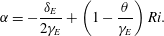 $$\begin{eqnarray}\unicode[STIX]{x1D6FC}=-\frac{\unicode[STIX]{x1D6FF}_{E}}{2\unicode[STIX]{x1D6FE}_{E}}+\left(1-\frac{\unicode[STIX]{x1D703}}{\unicode[STIX]{x1D6FE}_{E}}\right)Ri.\end{eqnarray}$$
The parameters
 $\unicode[STIX]{x1D6FF}_{E}$
,
$\unicode[STIX]{x1D6FF}_{E}$
,
 $\unicode[STIX]{x1D6FE}_{E}$
and
$\unicode[STIX]{x1D6FE}_{E}$
and
 $\unicode[STIX]{x1D703}$
, defined in appendix A, correspond to the dimensionless production of turbulence kinetic energy, the dimensionless flux of mean kinetic energy and the dimensionless flux of buoyancy, respectively (note that
$\unicode[STIX]{x1D703}$
, defined in appendix A, correspond to the dimensionless production of turbulence kinetic energy, the dimensionless flux of mean kinetic energy and the dimensionless flux of buoyancy, respectively (note that
 $\unicode[STIX]{x1D6FE}_{E}$
,
$\unicode[STIX]{x1D6FE}_{E}$
,
 $\unicode[STIX]{x1D6FF}_{E}$
and
$\unicode[STIX]{x1D6FF}_{E}$
and
 $\unicode[STIX]{x1D703}$
correspond to
$\unicode[STIX]{x1D703}$
correspond to
 $\unicode[STIX]{x1D6FE}_{m}$
,
$\unicode[STIX]{x1D6FE}_{m}$
,
 $\unicode[STIX]{x1D6FF}_{m}$
and
$\unicode[STIX]{x1D6FF}_{m}$
and
 $\unicode[STIX]{x1D703}_{m}$
, respectively, in van Reeuwijk & Craske Reference van Reeuwijk and Craske2015). The Richardson number
$\unicode[STIX]{x1D703}_{m}$
, respectively, in van Reeuwijk & Craske Reference van Reeuwijk and Craske2015). The Richardson number
 $Ri$
quantifies the balance between buoyancy and inertia within the plume and will be defined precisely in § 2.2. Equation (1.2) indicates that turbulent entrainment depends on the Richardson number and that this mean-flow contribution is distinct from that associated with the production of turbulence kinetic energy. Despite significant scatter, measurements indicate a systematic difference in the entrainment coefficient between jets and plumes (see table 1) and an approximately invariant (independent of
$Ri$
quantifies the balance between buoyancy and inertia within the plume and will be defined precisely in § 2.2. Equation (1.2) indicates that turbulent entrainment depends on the Richardson number and that this mean-flow contribution is distinct from that associated with the production of turbulence kinetic energy. Despite significant scatter, measurements indicate a systematic difference in the entrainment coefficient between jets and plumes (see table 1) and an approximately invariant (independent of
 $Ri$
) spreading rate (van Reeuwijk & Craske Reference van Reeuwijk and Craske2015, and references therein). The latter observation corresponds to the approximate equality of the dimensionless turbulence production
$Ri$
) spreading rate (van Reeuwijk & Craske Reference van Reeuwijk and Craske2015, and references therein). The latter observation corresponds to the approximate equality of the dimensionless turbulence production
 $\unicode[STIX]{x1D6FF}_{E}$
in jets and plumes.
$\unicode[STIX]{x1D6FF}_{E}$
in jets and plumes.
The entrainment coefficient has a broader significance in characterising the behaviour of free-shear flows than the linkages between flow kinematics and flow energetics described above might imply. Entrainment determines the rate at which passive and active scalars are diluted as a plume mixes with its surroundings (van Reeuwijk et al. Reference van Reeuwijk, Salizzoni, Hunt and Craske2016) and therefore provides a conceptual and physical link between several plume integrals relating to scalar transport. Whilst van Reeuwijk & Craske (Reference van Reeuwijk and Craske2015) reported consistency requirements for entrainment from momentum and energy conservation, the present work focuses on entrainment relations that can be derived from scalar transport budgets.
1.3 Turbulent transport and entrainment
The turbulent Schmidt and Prandtl numbers quantify the turbulent transport of momentum relative to either the turbulent transport of a passive scalar or heat, respectively:
 $$\begin{eqnarray}Sc_{T}\equiv \frac{\unicode[STIX]{x1D708}_{T}}{D_{T}},\quad Pr_{T}\equiv \frac{\unicode[STIX]{x1D708}_{T}}{\unicode[STIX]{x1D705}_{T}},\end{eqnarray}$$
where
 $\unicode[STIX]{x1D708}_{T}$
is the eddy viscosity,
$\unicode[STIX]{x1D708}_{T}$
is the eddy viscosity,
 $D_{T}$
is the turbulent mass diffusivity and
$D_{T}$
is the turbulent mass diffusivity and
 $\unicode[STIX]{x1D705}_{T}$
is the turbulent thermal diffusivity. For the purposes of discussion, we distinguish the roles of passive and active scalars by associating buoyancy with temperature differences in the flow, rather than mass concentrations. Therefore we use
$\unicode[STIX]{x1D705}_{T}$
is the turbulent thermal diffusivity. For the purposes of discussion, we distinguish the roles of passive and active scalars by associating buoyancy with temperature differences in the flow, rather than mass concentrations. Therefore we use
 $Sc_{T}$
in the context of a passive scalar and
$Sc_{T}$
in the context of a passive scalar and
 $Pr_{T}$
in the case of an active scalar.
$Pr_{T}$
in the case of an active scalar.
Table 1. Experimental data for jets (top) and plumes (bottom);
 $\unicode[STIX]{x1D711}$
is the ratio of the width of the scalar profile to the width of the velocity profile,
$\unicode[STIX]{x1D711}$
is the ratio of the width of the scalar profile to the width of the velocity profile,
 $\unicode[STIX]{x1D6FC}$
is the entrainment coefficient and
$\unicode[STIX]{x1D6FC}$
is the entrainment coefficient and
 $Sc_{T}$
and
$Sc_{T}$
and
 $Pr_{T}$
are the turbulent Schmidt and Prandtl numbers corresponding to jets and plumes, respectively.
$Pr_{T}$
are the turbulent Schmidt and Prandtl numbers corresponding to jets and plumes, respectively.

a
These values are based on the maximum observed turbulent transport of momentum and buoyancy, in addition to the reported value of
 $\unicode[STIX]{x1D711}$
. See § 4 for further details.
$\unicode[STIX]{x1D711}$
. See § 4 for further details.
Experiments and direct simulations indicate that the turbulent Schmidt number
 $Sc_{T}$
and the turbulent Prandtl number
$Sc_{T}$
and the turbulent Prandtl number
 $Pr_{T}$
in jets and plumes, respectively, are less than one (see e.g. Chen & Rodi Reference Chen and Rodi1980; Pietri et al.
Reference Pietri, Amielh and Anselmet2000; Wang & Law Reference Wang and Law2002; Ezzamel et al.
Reference Ezzamel, Salizzoni and Hunt2015; van Reeuwijk et al.
Reference van Reeuwijk, Salizzoni, Hunt and Craske2016, and the experimental data in table 1). For jets it is well established that the observation
$Pr_{T}$
in jets and plumes, respectively, are less than one (see e.g. Chen & Rodi Reference Chen and Rodi1980; Pietri et al.
Reference Pietri, Amielh and Anselmet2000; Wang & Law Reference Wang and Law2002; Ezzamel et al.
Reference Ezzamel, Salizzoni and Hunt2015; van Reeuwijk et al.
Reference van Reeuwijk, Salizzoni, Hunt and Craske2016, and the experimental data in table 1). For jets it is well established that the observation
 $Sc_{T}<1$
is consistent with the ratio
$Sc_{T}<1$
is consistent with the ratio
 $\unicode[STIX]{x1D711}$
of the width of the scalar profile to the width of the velocity profile being greater than one (Chen & Rodi Reference Chen and Rodi1980; van Reeuwijk et al.
Reference van Reeuwijk, Salizzoni, Hunt and Craske2016). A similar approach has been used to explain why
$\unicode[STIX]{x1D711}$
of the width of the scalar profile to the width of the velocity profile being greater than one (Chen & Rodi Reference Chen and Rodi1980; van Reeuwijk et al.
Reference van Reeuwijk, Salizzoni, Hunt and Craske2016). A similar approach has been used to explain why
 $Pr_{T}<1$
in plumes (Carazzo, Kaminski & Tait Reference Carazzo, Kaminski and Tait2006; Ezzamel et al.
Reference Ezzamel, Salizzoni and Hunt2015). However, in plumes the velocity and buoyancy profiles are, on average, observed to be of approximately equal width (see
$Pr_{T}<1$
in plumes (Carazzo, Kaminski & Tait Reference Carazzo, Kaminski and Tait2006; Ezzamel et al.
Reference Ezzamel, Salizzoni and Hunt2015). However, in plumes the velocity and buoyancy profiles are, on average, observed to be of approximately equal width (see
 $\unicode[STIX]{x1D711}$
in table 1), which raises the question of (i) the origin of the observed value of
$\unicode[STIX]{x1D711}$
in table 1), which raises the question of (i) the origin of the observed value of
 $Pr_{T}<1$
in plumes and (ii) the actual relationship between
$Pr_{T}<1$
in plumes and (ii) the actual relationship between
 $\unicode[STIX]{x1D711}$
and
$\unicode[STIX]{x1D711}$
and
 $Pr_{T}$
in plumes. An objective of the present work is to establish this dependence in a precise way and explain how it relates to turbulent entrainment. In this regard, it is useful to outline the salient differences between jets and plumes, as established by the studies referenced in table 1:
$Pr_{T}$
in plumes. An objective of the present work is to establish this dependence in a precise way and explain how it relates to turbulent entrainment. In this regard, it is useful to outline the salient differences between jets and plumes, as established by the studies referenced in table 1:
-
(i) the entrainment coefficient is higher in plumes than it is in jets;
-
(ii) the spreading rate of the velocity field in jets and plumes are approximately equal;
-
(iii) in jets the spreading rate of a passive scalar field is wider than the velocity field;
-
(iv) in plumes the buoyancy and velocity profile have approximately equal width;
-
(v) the turbulent Schmidt/Prandtl numbers are less than one in jets/plumes.
The overall aim of this work is to link these observations using information from the governing equations; we will, for example, demonstrate that observations iii and iv imply v. Although the general framework relies only on self-similarity as an assumption, we will also point out several deductions that can be made when further assumptions about the flow are introduced. One such deduction is that for pure plumes with mean scalar and velocity profiles of Gaussian form and equal width, the turbulent Prandtl number is equal to
 $3/5$
.
$3/5$
.
In § 2 we discuss the governing equations and derive a system of entrainment relations that extend those presented in van Reeuwijk & Craske (Reference van Reeuwijk and Craske2015). In § 3 we simplify the entrainment relations by considering special cases, such as pure plumes, before linking the entrainment coefficient with the turbulent Schmidt and Prandtl numbers in § 4 and drawing conclusions in § 5.
2 Governing integral relations
2.1 Mean buoyancy
We consider the flow in a statistically steady incompressible axisymmetric plume, whose ensemble-averaged velocity field
 $\overline{\boldsymbol{u}}=(\overline{u},\overline{v},\overline{w})$
is therefore constrained to satisfy
$\overline{\boldsymbol{u}}=(\overline{u},\overline{v},\overline{w})$
is therefore constrained to satisfy
 $$\begin{eqnarray}\unicode[STIX]{x1D735}\boldsymbol{\cdot }\overline{\boldsymbol{u}}=0.\end{eqnarray}$$
The equations governing momentum and the mean kinetic energy in a plume were discussed in van Reeuwijk & Craske (Reference van Reeuwijk and Craske2015); here we focus on the budgets associated with buoyancy, which in the case of jets corresponds to a passive scalar quantity. For a turbulent plume at high Reynolds number, the budget for mean buoyancy in the plume is expressed to leading order as
 $$\begin{eqnarray}\frac{1}{r}\frac{\unicode[STIX]{x2202}(r\overline{u}\,\overline{b})}{\unicode[STIX]{x2202}r}+\frac{\unicode[STIX]{x2202}(\overline{w}\overline{b})}{\unicode[STIX]{x2202}z}+\frac{1}{r}\frac{\unicode[STIX]{x2202}(r\overline{u^{\prime }b^{\prime }})}{\unicode[STIX]{x2202}r}=-\overline{w}N^{2},\end{eqnarray}$$
where
 $(r,z)$
are cylindrical coordinates and
$(r,z)$
are cylindrical coordinates and
 $b\equiv g(\unicode[STIX]{x1D70C}_{e}-\unicode[STIX]{x1D70C})/\unicode[STIX]{x1D70C}_{0}$
and
$b\equiv g(\unicode[STIX]{x1D70C}_{e}-\unicode[STIX]{x1D70C})/\unicode[STIX]{x1D70C}_{0}$
and
 $N^{2}\equiv -g\unicode[STIX]{x2202}_{z}\unicode[STIX]{x1D70C}_{e}/\unicode[STIX]{x1D70C}_{0}$
are the buoyancy and buoyancy frequency associated with the environment density
$N^{2}\equiv -g\unicode[STIX]{x2202}_{z}\unicode[STIX]{x1D70C}_{e}/\unicode[STIX]{x1D70C}_{0}$
are the buoyancy and buoyancy frequency associated with the environment density
 $\unicode[STIX]{x1D70C}_{e}(z)$
, reference density
$\unicode[STIX]{x1D70C}_{e}(z)$
, reference density
 $\unicode[STIX]{x1D70C}_{0}$
and local density
$\unicode[STIX]{x1D70C}_{0}$
and local density
 $\unicode[STIX]{x1D70C}$
. An equation for the squared mean buoyancy
$\unicode[STIX]{x1D70C}$
. An equation for the squared mean buoyancy
 $\overline{b}^{2}$
can be obtained by multiplying (2.2) by
$\overline{b}^{2}$
can be obtained by multiplying (2.2) by
 $2\overline{b}$
and using (2.1):
$2\overline{b}$
and using (2.1):
 $$\begin{eqnarray}\frac{1}{r}\frac{\unicode[STIX]{x2202}(r\overline{u}\,\overline{b}^{2})}{\unicode[STIX]{x2202}r}+\frac{\unicode[STIX]{x2202}\overline{w}\overline{b}^{2}}{\unicode[STIX]{x2202}z}+\frac{2}{r}\frac{\unicode[STIX]{x2202}(r\overline{u^{\prime }b^{\prime }}\,\overline{b})}{\unicode[STIX]{x2202}r}=\underbrace{2\,\overline{u^{\prime }b^{\prime }}\frac{\unicode[STIX]{x2202}\overline{b}}{\unicode[STIX]{x2202}r}}_{(a)}-\underbrace{2\overline{w}\overline{b}N^{2}}_{(b)}.\end{eqnarray}$$
Typically, the squared mean buoyancy
 $\overline{b}^{2}$
is reduced by
$\overline{b}^{2}$
is reduced by
 $(a)$
the production of buoyancy variance
$(a)$
the production of buoyancy variance
 $\overline{{b^{\prime }}^{2}}$
(term
$\overline{{b^{\prime }}^{2}}$
(term
 $(a)$
is a source in the budget for
$(a)$
is a source in the budget for
 $\overline{{b^{\prime }}^{2}}$
) and
$\overline{{b^{\prime }}^{2}}$
) and
 $(b)$
a (stable) background stratification. If
$(b)$
a (stable) background stratification. If
 $b$
is interpreted as a passive scalar concentration then
$b$
is interpreted as a passive scalar concentration then
 $N\equiv 0$
in equations (2.2) and (2.3).
$N\equiv 0$
in equations (2.2) and (2.3).
Integration of (2.2) and (2.3) with respect to
 $r$
from zero to infinity results in
$r$
from zero to infinity results in
 $$\begin{eqnarray}\displaystyle & \displaystyle \frac{\text{d}}{\text{d}z}\left(\unicode[STIX]{x1D703}\frac{BM}{Q}\right)=-QN^{2}, & \displaystyle\end{eqnarray}$$
 $$\begin{eqnarray}\displaystyle & \displaystyle \frac{\text{d}}{\text{d}z}\left(\unicode[STIX]{x1D6FE}_{S}\frac{B^{2}M^{2}}{Q^{3}}\right)=\unicode[STIX]{x1D6FF}_{S}\frac{B^{2}M^{5/2}}{Q^{4}}-2\unicode[STIX]{x1D703}\frac{BM}{Q}N^{2}, & \displaystyle\end{eqnarray}$$
where the volume flux, momentum flux and integral buoyancy in the plume are, respectively,
 $$\begin{eqnarray}Q\equiv 2\int _{0}^{\infty }\overline{w}r\,\text{d}r,\quad M\equiv 2\int _{0}^{\infty }\overline{w}^{2}r\,\text{d}r,\quad B\equiv 2\int _{0}^{\infty }\overline{b}r\,\text{d}r,\end{eqnarray}$$
and the dimensionless buoyancy flux
 $\unicode[STIX]{x1D703}$
, the dimensionless flux of mean squared buoyancy
$\unicode[STIX]{x1D703}$
, the dimensionless flux of mean squared buoyancy
 $\unicode[STIX]{x1D6FE}_{S}$
and the dimensionless production of buoyancy variance
$\unicode[STIX]{x1D6FE}_{S}$
and the dimensionless production of buoyancy variance
 $\unicode[STIX]{x1D6FF}_{S}$
are defined as
$\unicode[STIX]{x1D6FF}_{S}$
are defined as
 $$\begin{eqnarray}\displaystyle \unicode[STIX]{x1D703}\equiv \frac{2}{w_{m}b_{m}r_{m}^{2}}\int _{0}^{\infty }\!\overline{w}\overline{b}r\,\text{d}r,\quad \unicode[STIX]{x1D6FE}_{S}\equiv \frac{2}{w_{m}b_{m}^{2}r_{m}^{2}}\int _{0}^{\infty }\!\overline{w}\overline{b}^{2}r\,\text{d}r,\quad \unicode[STIX]{x1D6FF}_{S}\equiv \frac{4}{w_{m}b_{m}^{2}r_{m}}\int _{0}^{\infty }\overline{u^{\prime }b^{\prime }}\frac{\unicode[STIX]{x2202}\overline{b}}{\unicode[STIX]{x2202}r}r\,\text{d}r. & & \displaystyle \nonumber\\ \displaystyle & & \displaystyle\end{eqnarray}$$
Consequently, velocity, buoyancy and length scales for the flow at a given height can be defined according to
 $w_{m}\equiv M/Q$
,
$w_{m}\equiv M/Q$
,
 $b_{m}\equiv BM/Q^{2}$
and
$b_{m}\equiv BM/Q^{2}$
and
 $r_{m}\equiv Q/M^{1/2}$
, respectively. The integral equations corresponding to (2.4) and (2.5) that one obtains by integrating local equations for momentum and mean kinetic energy (which is dominated by the behaviour of the squared vertical velocity), in addition to the profile coefficients
$r_{m}\equiv Q/M^{1/2}$
, respectively. The integral equations corresponding to (2.4) and (2.5) that one obtains by integrating local equations for momentum and mean kinetic energy (which is dominated by the behaviour of the squared vertical velocity), in addition to the profile coefficients
 $\unicode[STIX]{x1D6FE}_{E}$
and
$\unicode[STIX]{x1D6FE}_{E}$
and
 $\unicode[STIX]{x1D6FF}_{E}$
, are summarised in appendix A. Hereafter we will assume that the flow is self-similar, which means that the dimensionless coefficients
$\unicode[STIX]{x1D6FF}_{E}$
, are summarised in appendix A. Hereafter we will assume that the flow is self-similar, which means that the dimensionless coefficients
 $\unicode[STIX]{x1D6FE}_{E}$
,
$\unicode[STIX]{x1D6FE}_{E}$
,
 $\unicode[STIX]{x1D6FF}_{E}$
,
$\unicode[STIX]{x1D6FF}_{E}$
,
 $\unicode[STIX]{x1D6FE}_{S}$
,
$\unicode[STIX]{x1D6FE}_{S}$
,
 $\unicode[STIX]{x1D6FF}_{S}$
and
$\unicode[STIX]{x1D6FF}_{S}$
and
 $\unicode[STIX]{x1D703}$
are constants. We discuss the implications of self-similarity in greater detail in § 3.3.
$\unicode[STIX]{x1D703}$
are constants. We discuss the implications of self-similarity in greater detail in § 3.3.
2.2 Entrainment relations
At this point we make use of the following fact: the local budgets pertaining to buoyancy or passive scalar quantities, equations (2.2) and (2.3), implicitly satisfy the constraint
 $\unicode[STIX]{x1D735}\boldsymbol{\cdot }\overline{\boldsymbol{u}}=0$
, which means that the corresponding integral budgets, equations (2.4) and (2.5), can be related to the entrainment coefficient
$\unicode[STIX]{x1D735}\boldsymbol{\cdot }\overline{\boldsymbol{u}}=0$
, which means that the corresponding integral budgets, equations (2.4) and (2.5), can be related to the entrainment coefficient
 $\unicode[STIX]{x1D6FC}$
. Applying the product rule to the left-hand side of (2.5) and substituting (2.4) yields an equation for the volume flux:
$\unicode[STIX]{x1D6FC}$
. Applying the product rule to the left-hand side of (2.5) and substituting (2.4) yields an equation for the volume flux:
 $$\begin{eqnarray}\frac{\text{d}Q}{\text{d}z}=-\frac{\unicode[STIX]{x1D6FF}_{S}}{\unicode[STIX]{x1D6FE}_{S}}M^{1/2}-\left(\frac{2}{\unicode[STIX]{x1D703}}-\frac{2\unicode[STIX]{x1D703}}{\unicode[STIX]{x1D6FE}_{S}}\right)\frac{N^{2}Q^{3}}{MB}.\end{eqnarray}$$
Comparison of (2.8) with (1.1) and (1.2) indicates that there are two equivalent ways of expressing the entrainment coefficient:
 $$\begin{eqnarray}\unicode[STIX]{x1D6FC}=\left\{\begin{array}{@{}l@{}}\displaystyle -\frac{\unicode[STIX]{x1D6FF}_{S}}{2\unicode[STIX]{x1D6FE}_{S}}-\left(\frac{1}{\unicode[STIX]{x1D703}}-\frac{\unicode[STIX]{x1D703}}{\unicode[STIX]{x1D6FE}_{S}}\right)\frac{Ri_{N}}{Ri},\quad \\ \displaystyle -\frac{\unicode[STIX]{x1D6FF}_{E}}{2\unicode[STIX]{x1D6FE}_{E}}+\left(1-\frac{\unicode[STIX]{x1D703}}{\unicode[STIX]{x1D6FE}_{E}}\right)Ri,\quad \end{array}\right.\end{eqnarray}$$
where
 $$\begin{eqnarray}Ri\equiv \frac{BQ}{M^{3/2}},\quad Ri_{N}\equiv \frac{N^{2}Q^{4}}{M^{3}}.\end{eqnarray}$$
Whereas
 $Ri$
is a Richardson number that characterises the role of buoyancy relative to inertia within the plume,
$Ri$
is a Richardson number that characterises the role of buoyancy relative to inertia within the plume,
 $Ri_{N}$
is a Richardson number associated with the environment, conveniently understood as the squared ratio of the plume’s time scale to that of the environment such that
$Ri_{N}$
is a Richardson number associated with the environment, conveniently understood as the squared ratio of the plume’s time scale to that of the environment such that
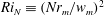 $Ri_{N}\equiv (Nr_{m}/w_{m})^{2}$
.
$Ri_{N}\equiv (Nr_{m}/w_{m})^{2}$
.
Equations (2.9) link the entrainment coefficient with budgets for momentum, mean energy, mean buoyancy and mean buoyancy squared. They state that entrainment can be viewed as depending on either the production of buoyancy variance or the production of turbulence kinetic energy. In either case, the entrainment coefficient is also affected by buoyancy within the plume (characterised by
 $Ri$
) and, in the case of (2.9a
), the variation of buoyancy in the ambient (characterised by
$Ri$
) and, in the case of (2.9a
), the variation of buoyancy in the ambient (characterised by
 $Ri_{N}$
). Equations (2.9) are exact integral relations for self-similar solutions of the boundary layer equations. Observations not satisfying (2.9) are therefore indicative of either measurement error, deviations from self-similarity and/or the presence of higher-order transport terms (such as
$Ri_{N}$
). Equations (2.9) are exact integral relations for self-similar solutions of the boundary layer equations. Observations not satisfying (2.9) are therefore indicative of either measurement error, deviations from self-similarity and/or the presence of higher-order transport terms (such as
 $\overline{w^{\prime }b^{\prime }}$
) that are not included in the boundary layer equations (2.2) (see e.g. van Reeuwijk & Craske Reference van Reeuwijk and Craske2015). We defer further interpretation of (2.9) until the next section, in which we focus on special cases.
$\overline{w^{\prime }b^{\prime }}$
) that are not included in the boundary layer equations (2.2) (see e.g. van Reeuwijk & Craske Reference van Reeuwijk and Craske2015). We defer further interpretation of (2.9) until the next section, in which we focus on special cases.
3 Special cases
In this section we analyse the relations (2.9) in detail by considering jets (
 $Ri=0$
,
$Ri=0$
,
 $Ri_{N}=0$
), pure plumes (
$Ri_{N}=0$
), pure plumes (
 $Ri\neq 0$
,
$Ri\neq 0$
,
 $Ri_{N}=0$
) and plumes that are either heated or placed in a stratified environment (
$Ri_{N}=0$
) and plumes that are either heated or placed in a stratified environment (
 $Ri\neq 0$
,
$Ri\neq 0$
,
 $Ri_{N}\neq 0$
). In the case of jets and pure plumes we compare (2.9) to observations from experiments and simulations, and obtain simplified versions of (2.9) for velocity and buoyancy profiles that have particular shapes.
$Ri_{N}\neq 0$
). In the case of jets and pure plumes we compare (2.9) to observations from experiments and simulations, and obtain simplified versions of (2.9) for velocity and buoyancy profiles that have particular shapes.
For comparison, we focus on the experiments by Wang & Law (Reference Wang and Law2002) in preference to the remaining experiments from table 1; we do this for three reasons. First, Wang & Law (Reference Wang and Law2002) provide observations of both jets and plumes in a single study. Secondly, the data contain significantly less scatter than previous observations. Thirdly, Wang & Law (Reference Wang and Law2002) provide analytical expressions for the observed radial dependence of all quantities, which allows us to make a consistent comparison with data from direct numerical simulation and the theory described in § 2.2.
The direct numerical simulations to which we compare our predictions were conducted on an open domain of dimensions
 $40^{2}\times 60$
source radii, discretised using
$40^{2}\times 60$
source radii, discretised using
 $1280^{2}\times 1920$
computational control volumes. The jet and plume have a Reynolds number at their source of 5000 and 1667, respectively, the latter increasing with respect to
$1280^{2}\times 1920$
computational control volumes. The jet and plume have a Reynolds number at their source of 5000 and 1667, respectively, the latter increasing with respect to
 $z$
. Further details and a discussion of the results can be found in van Reeuwijk et al. (Reference van Reeuwijk, Salizzoni, Hunt and Craske2016).
$z$
. Further details and a discussion of the results can be found in van Reeuwijk et al. (Reference van Reeuwijk, Salizzoni, Hunt and Craske2016).
3.1 Jets
Jets are neutrally buoyant; hence
 $Ri\equiv 0$
,
$Ri\equiv 0$
,
 $Ri_{N}\equiv 0$
and (2.9) become
$Ri_{N}\equiv 0$
and (2.9) become
 $$\begin{eqnarray}\unicode[STIX]{x1D6FC}=-\frac{\unicode[STIX]{x1D6FF}_{S}}{2\unicode[STIX]{x1D6FE}_{S}}=-\frac{\unicode[STIX]{x1D6FF}_{E}}{2\unicode[STIX]{x1D6FE}_{E}}.\end{eqnarray}$$
Equations (3.1) state that the dimensionless production of scalar variance
 $\unicode[STIX]{x1D6FF}_{S}$
is equal to the dimensionless production of turbulence kinetic energy
$\unicode[STIX]{x1D6FF}_{S}$
is equal to the dimensionless production of turbulence kinetic energy
 $\unicode[STIX]{x1D6FF}_{E}$
, when each of the quantities involved is normalised by the corresponding transport coefficients
$\unicode[STIX]{x1D6FF}_{E}$
, when each of the quantities involved is normalised by the corresponding transport coefficients
 $\unicode[STIX]{x1D6FE}_{S}$
and
$\unicode[STIX]{x1D6FE}_{S}$
and
 $\unicode[STIX]{x1D6FE}_{E}$
. Physically this means that entrainment is proportional to the production of scalar variance
$\unicode[STIX]{x1D6FE}_{E}$
. Physically this means that entrainment is proportional to the production of scalar variance
 $\overline{{b^{\prime }}^{2}}$
, which is consistent with the phenomenological view that entrainment is responsible for dilution. In the absence of buoyancy, the budgets related to the mean velocity
$\overline{{b^{\prime }}^{2}}$
, which is consistent with the phenomenological view that entrainment is responsible for dilution. In the absence of buoyancy, the budgets related to the mean velocity
 $\overline{w}$
and the mean buoyancy
$\overline{w}$
and the mean buoyancy
 $\overline{b}$
have the same form, which accounts for the identical form of the equalities in (3.1). Consequently, the ratio of scalar variance production and turbulence kinetic energy production is equal to the ratio of the corresponding mean energy fluxes:
$\overline{b}$
have the same form, which accounts for the identical form of the equalities in (3.1). Consequently, the ratio of scalar variance production and turbulence kinetic energy production is equal to the ratio of the corresponding mean energy fluxes:
 $$\begin{eqnarray}\frac{\unicode[STIX]{x1D6FF}_{S}}{\unicode[STIX]{x1D6FF}_{E}}=\frac{\unicode[STIX]{x1D6FE}_{S}}{\unicode[STIX]{x1D6FE}_{E}}.\end{eqnarray}$$
As discussed in § 1.3, observations of jets suggest that the mean scalar profile is wider than the mean velocity profile, i.e. the ratio of the widths
 $\unicode[STIX]{x1D711}>1$
. This implies that, in the mean, a relatively large proportion of the scalar distribution is transported by relatively small velocities. This in turn means that the dimensionless flux of mean buoyancy squared
$\unicode[STIX]{x1D711}>1$
. This implies that, in the mean, a relatively large proportion of the scalar distribution is transported by relatively small velocities. This in turn means that the dimensionless flux of mean buoyancy squared
 $\unicode[STIX]{x1D6FE}_{S}$
is less than that of mean kinetic energy
$\unicode[STIX]{x1D6FE}_{S}$
is less than that of mean kinetic energy
 $\unicode[STIX]{x1D6FE}_{E}$
. In order to balance these fluxes, the production of turbulence kinetic energy has a larger magnitude than that of buoyancy variance, as predicted by (3.2).
$\unicode[STIX]{x1D6FE}_{E}$
. In order to balance these fluxes, the production of turbulence kinetic energy has a larger magnitude than that of buoyancy variance, as predicted by (3.2).
Table 2. Integral quantities and estimates of the turbulent Schmidt and Prandtl numbers in a pure plume and a pure jet using the direct numerical simulation data presented in van Reeuwijk et al. (Reference van Reeuwijk, Salizzoni, Hunt and Craske2016) and the experimental data presented in Wang & Law (Reference Wang and Law2002).
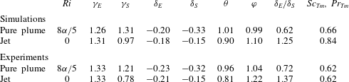
Table 2 provides detailed information relating to the profile coefficients observed in jets and pure plumes from experiments (Wang & Law Reference Wang and Law2002) and simulations (van Reeuwijk et al.
Reference van Reeuwijk, Salizzoni, Hunt and Craske2016). The simulation data and the experimental data are consistent with the view that in jets
 $\unicode[STIX]{x1D6FE}_{S}<\unicode[STIX]{x1D6FE}_{E}$
and that consequently
$\unicode[STIX]{x1D6FE}_{S}<\unicode[STIX]{x1D6FE}_{E}$
and that consequently
 $-\unicode[STIX]{x1D6FF}_{S}<-\unicode[STIX]{x1D6FF}_{E}$
. However, there is a mismatch between the experimentally observed ratios
$-\unicode[STIX]{x1D6FF}_{S}<-\unicode[STIX]{x1D6FF}_{E}$
. However, there is a mismatch between the experimentally observed ratios
 $-\unicode[STIX]{x1D6FF}_{E}/2\unicode[STIX]{x1D6FE}_{E}=0.079$
and
$-\unicode[STIX]{x1D6FF}_{E}/2\unicode[STIX]{x1D6FE}_{E}=0.079$
and
 $-\unicode[STIX]{x1D6FF}_{S}/2\unicode[STIX]{x1D6FE}_{S}=0.096$
in jets, which is inconsistent with (3.1). As mentioned in § 2.2, because (3.1) is an exact integral statement about the boundary layer equations, we attribute deviations from (3.1) to experimental uncertainty or the effects of higher-order transport terms that were not included in the boundary layer equations (2.2).
$-\unicode[STIX]{x1D6FF}_{S}/2\unicode[STIX]{x1D6FE}_{S}=0.096$
in jets, which is inconsistent with (3.1). As mentioned in § 2.2, because (3.1) is an exact integral statement about the boundary layer equations, we attribute deviations from (3.1) to experimental uncertainty or the effects of higher-order transport terms that were not included in the boundary layer equations (2.2).
3.2 Pure plumes
In a pure plume, the buoyancy flux is a conserved quantity because
 $N\equiv 0$
; hence
$N\equiv 0$
; hence
 $Ri_{N}\equiv 0$
and
$Ri_{N}\equiv 0$
and
 $Ri$
is a known positive constant. The relations (2.9) therefore become
$Ri$
is a known positive constant. The relations (2.9) therefore become
 $$\begin{eqnarray}\unicode[STIX]{x1D6FC}=-\frac{\unicode[STIX]{x1D6FF}_{S}}{2\unicode[STIX]{x1D6FE}_{S}}=-\frac{\unicode[STIX]{x1D6FF}_{E}}{2\unicode[STIX]{x1D6FE}_{E}}+\left(1-\frac{\unicode[STIX]{x1D703}}{\unicode[STIX]{x1D6FE}_{E}}\right)Ri.\end{eqnarray}$$
With the addition of forcing from buoyancy in the plume, the form of the budgets associated with mean velocity differ from those associated with mean buoyancy; consequently the two equalities for
 $\unicode[STIX]{x1D6FC}$
in (3.3) also have a different form.
$\unicode[STIX]{x1D6FC}$
in (3.3) also have a different form.
The final terms in (3.3) provide a representation of entrainment in terms of the energetics of the mean flow. Like buoyancy, the momentum is also ‘diluted’ by entrainment. In energetic terms this effect is expressed by
 $-\unicode[STIX]{x1D6FF}_{E}/2\unicode[STIX]{x1D6FE}_{E}$
, which indicates that entrainment corresponds to the production of turbulence kinetic energy. However, the velocity field is also modified by buoyancy; hence a simple conclusion that can be drawn from (3.3) is that although the entrainment coefficient is proportional to buoyancy variance production, it is not (necessarily) proportional to turbulence kinetic energy production. The difference between these two perspectives is accounted for in the final term of (3.3), by a contribution to entrainment that depends on the forcing provided by buoyancy and therefore the Richardson number
$-\unicode[STIX]{x1D6FF}_{E}/2\unicode[STIX]{x1D6FE}_{E}$
, which indicates that entrainment corresponds to the production of turbulence kinetic energy. However, the velocity field is also modified by buoyancy; hence a simple conclusion that can be drawn from (3.3) is that although the entrainment coefficient is proportional to buoyancy variance production, it is not (necessarily) proportional to turbulence kinetic energy production. The difference between these two perspectives is accounted for in the final term of (3.3), by a contribution to entrainment that depends on the forcing provided by buoyancy and therefore the Richardson number
 $Ri$
, as discussed in Kaminski et al. (Reference Kaminski, Tait and Carazzo2005) and van Reeuwijk & Craske (Reference van Reeuwijk and Craske2015).
$Ri$
, as discussed in Kaminski et al. (Reference Kaminski, Tait and Carazzo2005) and van Reeuwijk & Craske (Reference van Reeuwijk and Craske2015).
For pure plumes the exact relationship between the Richardson number and the entrainment coefficient is
 $Ri=8\unicode[STIX]{x1D6FC}/5$
(Morton & Middleton Reference Morton and Middleton1973; Hunt & Kaye Reference Hunt and Kaye2005; van Reeuwijk & Craske Reference van Reeuwijk and Craske2015); hence (3.3) implies that the production of buoyancy variance and turbulence kinetic energy in a pure plume are related according to
$Ri=8\unicode[STIX]{x1D6FC}/5$
(Morton & Middleton Reference Morton and Middleton1973; Hunt & Kaye Reference Hunt and Kaye2005; van Reeuwijk & Craske Reference van Reeuwijk and Craske2015); hence (3.3) implies that the production of buoyancy variance and turbulence kinetic energy in a pure plume are related according to
 $$\begin{eqnarray}\frac{\unicode[STIX]{x1D6FF}_{E}}{\unicode[STIX]{x1D6FE}_{E}}=\frac{8}{5}\left(\frac{\unicode[STIX]{x1D703}}{\unicode[STIX]{x1D6FE}_{E}}-\frac{3}{8}\right)\frac{\unicode[STIX]{x1D6FF}_{S}}{\unicode[STIX]{x1D6FE}_{S}}.\end{eqnarray}$$
Unlike jets, scalar (buoyancy) and velocity profiles in pure plumes are observed to have approximately equal width (see e.g.
 $\unicode[STIX]{x1D711}$
in tables 1 and 2), which implies that
$\unicode[STIX]{x1D711}$
in tables 1 and 2), which implies that
 $\unicode[STIX]{x1D6FE}_{E}=\unicode[STIX]{x1D6FE}_{S}$
and
$\unicode[STIX]{x1D6FE}_{E}=\unicode[STIX]{x1D6FE}_{S}$
and
 $\unicode[STIX]{x1D703}=1$
. If, in addition, it is assumed that the buoyancy and velocity profiles have a Gaussian form then
$\unicode[STIX]{x1D703}=1$
. If, in addition, it is assumed that the buoyancy and velocity profiles have a Gaussian form then
 $\unicode[STIX]{x1D6FE}_{S}=\unicode[STIX]{x1D6FE}_{E}=4/3$
(Craske & van Reeuwijk Reference Craske and van Reeuwijk2015) and
$\unicode[STIX]{x1D6FE}_{S}=\unicode[STIX]{x1D6FE}_{E}=4/3$
(Craske & van Reeuwijk Reference Craske and van Reeuwijk2015) and
 $$\begin{eqnarray}\frac{\unicode[STIX]{x1D6FF}_{S}}{\unicode[STIX]{x1D6FF}_{E}}=\frac{5}{3},\end{eqnarray}$$
which means that the buoyancy variance production is larger than the turbulence kinetic energy production by a factor of
 $5/3$
. The physical explanation behind (3.5) is that although entrainment is concomitant with the conversion of
$5/3$
. The physical explanation behind (3.5) is that although entrainment is concomitant with the conversion of
 $\overline{w}^{2}$
and
$\overline{w}^{2}$
and
 $\overline{b}^{2}$
into
$\overline{b}^{2}$
into
 $\overline{{w^{\prime }}^{2}}$
and
$\overline{{w^{\prime }}^{2}}$
and
 $\overline{{b^{\prime }}^{2}}$
, respectively,
$\overline{{b^{\prime }}^{2}}$
, respectively,
 $\overline{w}$
and
$\overline{w}$
and
 $\overline{w}^{2}$
are forced, in a positive sense, by buoyancy; hence
$\overline{w}^{2}$
are forced, in a positive sense, by buoyancy; hence
 $0\leqslant -\unicode[STIX]{x1D6FF}_{E}\leqslant -\unicode[STIX]{x1D6FF}_{S}$
in general.
$0\leqslant -\unicode[STIX]{x1D6FF}_{E}\leqslant -\unicode[STIX]{x1D6FF}_{S}$
in general.
Figure 1 displays the radial dependence of quantities obtained from the direct numerical simulation of a pure plume (van Reeuwijk et al.
Reference van Reeuwijk, Salizzoni, Hunt and Craske2016). The profiles in thin grey lines correspond to longitudinal locations ranging from
 $20$
to
$20$
to
 $50$
source radii and the thick red and blue (light and dark, respectively) lines indicate averages associated with buoyancy and velocity, respectively. As is evident from figure 1(a), the profiles of velocity
$50$
source radii and the thick red and blue (light and dark, respectively) lines indicate averages associated with buoyancy and velocity, respectively. As is evident from figure 1(a), the profiles of velocity
 $\overline{w}$
and buoyancy
$\overline{w}$
and buoyancy
 $\overline{b}$
have a similar shape and radial extent and figure 1(b) suggests that in the radial direction the turbulent transport of buoyancy
$\overline{b}$
have a similar shape and radial extent and figure 1(b) suggests that in the radial direction the turbulent transport of buoyancy
 $\overline{u^{\prime }b^{\prime }}$
is approximately
$\overline{u^{\prime }b^{\prime }}$
is approximately
 $5/3$
times larger than the transport of momentum
$5/3$
times larger than the transport of momentum
 $\overline{u^{\prime }w^{\prime }}$
. Consequently, the production of turbulence kinetic energy is smaller than the production of buoyancy variance by a factor of
$\overline{u^{\prime }w^{\prime }}$
. Consequently, the production of turbulence kinetic energy is smaller than the production of buoyancy variance by a factor of
 $3/5$
for all
$3/5$
for all
 $r$
, as verified in figure 1(c), which is consistent with the integral relation (3.5).
$r$
, as verified in figure 1(c), which is consistent with the integral relation (3.5).
Figure 1 also includes data from the experiments of Wang & Law (Reference Wang and Law2002). Although the ratio between
 $\overline{u^{\prime }w^{\prime }}$
and
$\overline{u^{\prime }w^{\prime }}$
and
 $\overline{u^{\prime }b^{\prime }}$
is approximately
$\overline{u^{\prime }b^{\prime }}$
is approximately
 $3/5$
(figure 1
b), there is a small difference between the observed width of the mean buoyancy profile compared with the mean velocity profile in figure 1(a). Locally this results in a noticeable difference between the production terms from the experiments and the simulations (figure 1
c). However, as indicated in table 2, the effect that this has on the ratio of integrals
$3/5$
(figure 1
b), there is a small difference between the observed width of the mean buoyancy profile compared with the mean velocity profile in figure 1(a). Locally this results in a noticeable difference between the production terms from the experiments and the simulations (figure 1
c). However, as indicated in table 2, the effect that this has on the ratio of integrals
 $\unicode[STIX]{x1D6FF}_{S}/\unicode[STIX]{x1D6FF}_{E}\approx 5/3$
is relatively small.
$\unicode[STIX]{x1D6FF}_{S}/\unicode[STIX]{x1D6FF}_{E}\approx 5/3$
is relatively small.

Figure 1. Self-similar buoyancy and velocity fields in a turbulent plume: (a) mean (ensemble-averaged) quantities; (b) turbulent transport of momentum
 $\overline{u^{\prime }w^{\prime }}$
and buoyancy
$\overline{u^{\prime }w^{\prime }}$
and buoyancy
 $\overline{u^{\prime }b^{\prime }}$
in the radial direction; (c) the production of turbulence kinetic energy
$\overline{u^{\prime }b^{\prime }}$
in the radial direction; (c) the production of turbulence kinetic energy
 $\overline{u^{\prime }w^{\prime }}\unicode[STIX]{x2202}_{r}\overline{w}$
and buoyancy variance
$\overline{u^{\prime }w^{\prime }}\unicode[STIX]{x2202}_{r}\overline{w}$
and buoyancy variance
 $\overline{u^{\prime }b^{\prime }}\unicode[STIX]{x2202}_{r}\overline{b}$
. The solid lines were obtained from the dataset discussed in van Reeuwijk et al. (Reference van Reeuwijk, Salizzoni, Hunt and Craske2016) and the dotted lines from Wang & Law (Reference Wang and Law2002). The thin light grey lines refer to profiles obtained at a single height and the red/blue (light/dark) lines correspond to their average. The thin black line in (c) is the curve associated with buoyancy variance production reduced by a factor of
$\overline{u^{\prime }b^{\prime }}\unicode[STIX]{x2202}_{r}\overline{b}$
. The solid lines were obtained from the dataset discussed in van Reeuwijk et al. (Reference van Reeuwijk, Salizzoni, Hunt and Craske2016) and the dotted lines from Wang & Law (Reference Wang and Law2002). The thin light grey lines refer to profiles obtained at a single height and the red/blue (light/dark) lines correspond to their average. The thin black line in (c) is the curve associated with buoyancy variance production reduced by a factor of
 $3/5$
.
$3/5$
.
3.3 Lazy and forced plumes
Lazy (dominated by buoyancy) and forced (dominated by inertia) plumes have a Richardson number
 $Ri$
that is greater than or less than
$Ri$
that is greater than or less than
 $8\unicode[STIX]{x1D6FC}/5$
, respectively. Thus we imagine situations in which the right-hand side of the buoyancy budget (2.2) is non-zero but that the flow nevertheless maintains a constant Richardson number. Such situations correspond to similarity (power-law) solutions of the governing equations in which all dimensionless quantities are independent of
$8\unicode[STIX]{x1D6FC}/5$
, respectively. Thus we imagine situations in which the right-hand side of the buoyancy budget (2.2) is non-zero but that the flow nevertheless maintains a constant Richardson number. Such situations correspond to similarity (power-law) solutions of the governing equations in which all dimensionless quantities are independent of
 $z$
. In principle, the forcing term could result from a stratification of the environment or from an internal source of buoyancy, both cases resulting in
$z$
. In principle, the forcing term could result from a stratification of the environment or from an internal source of buoyancy, both cases resulting in
 $N^{2}\neq 0$
in (2.4) and (2.5). For these similarity solutions in which the plume is in ‘equilibrium’ with its surroundings,
$N^{2}\neq 0$
in (2.4) and (2.5). For these similarity solutions in which the plume is in ‘equilibrium’ with its surroundings,
 $Ri_{N}<0$
corresponds to a lazy plume (due to internal heating, for example) and
$Ri_{N}<0$
corresponds to a lazy plume (due to internal heating, for example) and
 $Ri_{N}>0$
corresponds to a forced plume (due to a stable stratification, for example).
$Ri_{N}>0$
corresponds to a forced plume (due to a stable stratification, for example).
The relationship between the destruction of either mean-flow energy or squared mean buoyancy and entrainment depends on the source term on the right-hand side of the buoyancy budget or the momentum budget. For example, as derived from the buoyancy budget and the mean buoyancy squared budget, the entrainment relation is (2.9a ):
 $$\begin{eqnarray}\unicode[STIX]{x1D6FC}=-\frac{\unicode[STIX]{x1D6FF}_{S}}{2\unicode[STIX]{x1D6FE}_{S}}-\left(\frac{1}{\unicode[STIX]{x1D703}}-\frac{\unicode[STIX]{x1D703}}{\unicode[STIX]{x1D6FE}_{S}}\right)\frac{Ri_{N}}{Ri}.\end{eqnarray}$$
An increase in
 $Ri_{N}$
is consistent with a decrease in
$Ri_{N}$
is consistent with a decrease in
 $\unicode[STIX]{x1D6FC}$
(entrainment) and/or an increase in
$\unicode[STIX]{x1D6FC}$
(entrainment) and/or an increase in
 $-\unicode[STIX]{x1D6FF}_{S}/2\unicode[STIX]{x1D6FE}_{S}$
(buoyancy variance production). In other words, as
$-\unicode[STIX]{x1D6FF}_{S}/2\unicode[STIX]{x1D6FE}_{S}$
(buoyancy variance production). In other words, as
 $Ri_{N}$
increases the ratio between buoyancy variance production and entrainment increases. Conversely, the entrainment relation (2.9b
) based on budgets for momentum and mean kinetic energy, states that as
$Ri_{N}$
increases the ratio between buoyancy variance production and entrainment increases. Conversely, the entrainment relation (2.9b
) based on budgets for momentum and mean kinetic energy, states that as
 $Ri$
decreases the ratio between turbulence kinetic energy production and entrainment increases. As evidenced by the dependence of
$Ri$
decreases the ratio between turbulence kinetic energy production and entrainment increases. As evidenced by the dependence of
 $\unicode[STIX]{x1D6FC}$
on
$\unicode[STIX]{x1D6FC}$
on
 $\unicode[STIX]{x1D703}$
and
$\unicode[STIX]{x1D703}$
and
 $\unicode[STIX]{x1D6FE}_{S}$
, the shapes and the relative widths of the buoyancy and velocity profiles play a crucial role in determining the link between entrainment, variance production terms and source terms.
$\unicode[STIX]{x1D6FE}_{S}$
, the shapes and the relative widths of the buoyancy and velocity profiles play a crucial role in determining the link between entrainment, variance production terms and source terms.
It is useful and physically meaningful to evaluate
 $Ri_{N}$
for a stratified environment with
$Ri_{N}$
for a stratified environment with
 $N^{2}\sim N_{0}^{2}z^{a}$
(cf. Batchelor Reference Batchelor1954; Caulfield & Woods Reference Caulfield and Woods1998). In that case
$N^{2}\sim N_{0}^{2}z^{a}$
(cf. Batchelor Reference Batchelor1954; Caulfield & Woods Reference Caulfield and Woods1998). In that case
 $Ri$
and
$Ri$
and
 $Ri_{N}$
are related to
$Ri_{N}$
are related to
 $a$
and
$a$
and
 $\unicode[STIX]{x1D6FC}$
according to (van Reeuwijk & Craske Reference van Reeuwijk and Craske2015)
$\unicode[STIX]{x1D6FC}$
according to (van Reeuwijk & Craske Reference van Reeuwijk and Craske2015)
 $$\begin{eqnarray}Ri=\frac{4a+16}{6+a}\unicode[STIX]{x1D6FC},\quad \frac{Ri_{N}}{Ri}=-\frac{6a+16}{6+a}\unicode[STIX]{x1D703}\unicode[STIX]{x1D6FC}.\end{eqnarray}$$
Using (2.9) and (3.7) and rearranging gives
 $$\begin{eqnarray}\frac{\unicode[STIX]{x1D6FF}_{S}}{\unicode[STIX]{x1D6FC}\unicode[STIX]{x1D6FE}_{S}}=\left(1-\frac{\unicode[STIX]{x1D703}^{2}}{\unicode[STIX]{x1D6FE}_{S}}\right)\left(\frac{12a+32}{6+a}\right)-2,\quad \frac{\unicode[STIX]{x1D6FF}_{E}}{\unicode[STIX]{x1D6FC}\unicode[STIX]{x1D6FE}_{E}}=\left(1-\frac{\unicode[STIX]{x1D703}}{\unicode[STIX]{x1D6FE}_{E}}\right)\left(\frac{8a+32}{6+a}\right)-2.\end{eqnarray}$$
If one assumes that
 $\unicode[STIX]{x1D703}=1$
and
$\unicode[STIX]{x1D703}=1$
and
 $\unicode[STIX]{x1D6FE}_{S}=\unicode[STIX]{x1D6FE}_{E}=4/3$
, in accordance with Gaussian profiles of equal width, then
$\unicode[STIX]{x1D6FE}_{S}=\unicode[STIX]{x1D6FE}_{E}=4/3$
, in accordance with Gaussian profiles of equal width, then
 $$\begin{eqnarray}\frac{\unicode[STIX]{x1D6FF}_{S}}{\unicode[STIX]{x1D6FC}}=\frac{4}{3}\left(\frac{a-4}{a+6}\right),\quad \frac{\unicode[STIX]{x1D6FF}_{E}}{\unicode[STIX]{x1D6FC}}=-\frac{4}{3}\left(\frac{4}{a+6}\right),\end{eqnarray}$$
and
 $$\begin{eqnarray}\frac{\unicode[STIX]{x1D6FF}_{S}}{\unicode[STIX]{x1D6FF}_{E}}=1-\frac{a}{4}.\end{eqnarray}$$
The relationship between
 $\unicode[STIX]{x1D6FF}_{E}/\unicode[STIX]{x1D6FC}$
and
$\unicode[STIX]{x1D6FF}_{E}/\unicode[STIX]{x1D6FC}$
and
 $\unicode[STIX]{x1D6FF}_{S}/\unicode[STIX]{x1D6FC}$
when
$\unicode[STIX]{x1D6FF}_{S}/\unicode[STIX]{x1D6FC}$
when
 $\unicode[STIX]{x1D6FE}_{E}=\unicode[STIX]{x1D6FE}_{S}=4/3$
and
$\unicode[STIX]{x1D6FE}_{E}=\unicode[STIX]{x1D6FE}_{S}=4/3$
and
 $\unicode[STIX]{x1D703}=1$
is shown in figure 2. For pure plumes,
$\unicode[STIX]{x1D703}=1$
is shown in figure 2. For pure plumes,
 $a=-8/3$
, and the production of buoyancy variance is
$a=-8/3$
, and the production of buoyancy variance is
 $5/3$
times larger than the production of turbulence kinetic energy, as established in § 3.2. To extend the arguments made above, we note that as the exponent
$5/3$
times larger than the production of turbulence kinetic energy, as established in § 3.2. To extend the arguments made above, we note that as the exponent
 $a$
becomes more negative, equations (3.7) imply that
$a$
becomes more negative, equations (3.7) imply that
 $Ri_{N}/Ri$
increases more rapidly than
$Ri_{N}/Ri$
increases more rapidly than
 $Ri$
decreases. Consequently, for profiles of a fixed shape, the production of buoyancy variance must increase relative to the production of turbulence kinetic energy according to (3.10). The limits
$Ri$
decreases. Consequently, for profiles of a fixed shape, the production of buoyancy variance must increase relative to the production of turbulence kinetic energy according to (3.10). The limits
 $a\rightarrow -4$
and
$a\rightarrow -4$
and
 $Ri\rightarrow 0$
corresponds to a jet, wherein entrainment can be equated entirely with the production of turbulence kinetic energy.
$Ri\rightarrow 0$
corresponds to a jet, wherein entrainment can be equated entirely with the production of turbulence kinetic energy.

Figure 2. The relationship between
 $-\unicode[STIX]{x1D6FF}_{E}/\unicode[STIX]{x1D6FC}$
(thick dark/blue) and
$-\unicode[STIX]{x1D6FF}_{E}/\unicode[STIX]{x1D6FC}$
(thick dark/blue) and
 $-\unicode[STIX]{x1D6FF}_{S}/\unicode[STIX]{x1D6FC}$
(thick dashed light/red) in a heated/cooled plume or a plume in a stratified environment
$-\unicode[STIX]{x1D6FF}_{S}/\unicode[STIX]{x1D6FC}$
(thick dashed light/red) in a heated/cooled plume or a plume in a stratified environment
 $N^{2}\sim z^{a}$
. A given exponent
$N^{2}\sim z^{a}$
. A given exponent
 $a$
implies a ratio of
$a$
implies a ratio of
 $Ri_{N}/Ri$
to
$Ri_{N}/Ri$
to
 $Ri$
, according to (3.7). The constant
$Ri$
, according to (3.7). The constant
 $-\unicode[STIX]{x1D6FF}_{S}/\unicode[STIX]{x1D6FC}=8/3$
, corresponding to a passive scalar, is denoted by the thick horizontal grey line and the ratio
$-\unicode[STIX]{x1D6FF}_{S}/\unicode[STIX]{x1D6FC}=8/3$
, corresponding to a passive scalar, is denoted by the thick horizontal grey line and the ratio
 $\unicode[STIX]{x1D6FF}_{S}/\unicode[STIX]{x1D6FF}_{E}$
is denoted by the thin black line.
$\unicode[STIX]{x1D6FF}_{S}/\unicode[STIX]{x1D6FF}_{E}$
is denoted by the thin black line.
An important point to bear in mind when interpreting figure 2 is that the budget for a passive scalar is not directly affected by the value of
 $Ri_{N}$
or
$Ri_{N}$
or
 $Ri$
and therefore continues to imply the entrainment relation (3.3) derived in § 3.2 for a pure plume. Thus, for constant
$Ri$
and therefore continues to imply the entrainment relation (3.3) derived in § 3.2 for a pure plume. Thus, for constant
 $\unicode[STIX]{x1D6FE}_{S}$
the production of passive scalar variance relative to the entrainment coefficient is constant, as indicated by the thick grey line in figure 2. Pure plumes are therefore a special case, because
$\unicode[STIX]{x1D6FE}_{S}$
the production of passive scalar variance relative to the entrainment coefficient is constant, as indicated by the thick grey line in figure 2. Pure plumes are therefore a special case, because
 $Ri_{N}=0$
implies that the buoyancy equation is identical to the equation satisfied by a passive scalar. Only in that particular case does the production of buoyancy variance equal that of passive scalar variance, as indicated by the point
$Ri_{N}=0$
implies that the buoyancy equation is identical to the equation satisfied by a passive scalar. Only in that particular case does the production of buoyancy variance equal that of passive scalar variance, as indicated by the point
 $(-8/3,8/3)$
in figure 2. In stably stratified environments the production of buoyancy variance in a Gaussian plume is necessarily greater than the production of passive scalar variance due to the negative forcing that appears in the buoyancy budgets.
$(-8/3,8/3)$
in figure 2. In stably stratified environments the production of buoyancy variance in a Gaussian plume is necessarily greater than the production of passive scalar variance due to the negative forcing that appears in the buoyancy budgets.
On the right-hand side of figure 2,
 $a\rightarrow 0$
and
$a\rightarrow 0$
and
 $Ri\rightarrow 8\unicode[STIX]{x1D6FC}/3$
, which represents a plume with an internal buoyancy flux gain, characterised by equal values of
$Ri\rightarrow 8\unicode[STIX]{x1D6FC}/3$
, which represents a plume with an internal buoyancy flux gain, characterised by equal values of
 $Ri$
and
$Ri$
and
 $Ri_{N}/Ri$
(cf. Hunt & Kaye Reference Hunt and Kaye2005, who considered the case of linear internal buoyancy flux gain, corresponding to
$Ri_{N}/Ri$
(cf. Hunt & Kaye Reference Hunt and Kaye2005, who considered the case of linear internal buoyancy flux gain, corresponding to
 $a=-2$
). In the limit
$a=-2$
). In the limit
 $a\rightarrow 0$
, the mean kinetic energy budget and the squared mean buoyancy budget (2.3) are equivalent in how they relate to volume conservation; hence
$a\rightarrow 0$
, the mean kinetic energy budget and the squared mean buoyancy budget (2.3) are equivalent in how they relate to volume conservation; hence
 $\unicode[STIX]{x1D6FF}_{E}=\unicode[STIX]{x1D6FF}_{S}$
. On the other hand, the production of a passive scalar’s variance, which is not directly influenced by buoyancy, is significantly larger than the production of turbulence kinetic energy and buoyancy variance.
$\unicode[STIX]{x1D6FF}_{E}=\unicode[STIX]{x1D6FF}_{S}$
. On the other hand, the production of a passive scalar’s variance, which is not directly influenced by buoyancy, is significantly larger than the production of turbulence kinetic energy and buoyancy variance.
4 The turbulent Schmidt and Prandtl numbers
The turbulent Schmidt and Prandtl numbers relate the turbulent transport of momentum to that of either heat (buoyancy) or a passive scalar, respectively, and are defined as field variables according to the ratio of the eddy viscosity
 $\unicode[STIX]{x1D708}_{T}$
to the diffusivity of either heat or mass:
$\unicode[STIX]{x1D708}_{T}$
to the diffusivity of either heat or mass:
 $$\begin{eqnarray}Pr_{T}\equiv \frac{\unicode[STIX]{x1D708}_{T}}{\unicode[STIX]{x1D705}_{T}}=\frac{\overline{u^{\prime }w^{\prime }}}{\overline{u^{\prime }b^{\prime }}}\left({\displaystyle \frac{\unicode[STIX]{x2202}\overline{b}}{\unicode[STIX]{x2202}r}}\right)\left({\displaystyle \frac{\unicode[STIX]{x2202}\overline{w}}{\unicode[STIX]{x2202}r}}\right)^{-1}.\end{eqnarray}$$
The definition for the turbulent Schmidt number
 $Sc_{T}$
is analogous to (4.1), with the thermal diffusivity
$Sc_{T}$
is analogous to (4.1), with the thermal diffusivity
 $\unicode[STIX]{x1D705}_{T}$
replaced with the mass diffusivity
$\unicode[STIX]{x1D705}_{T}$
replaced with the mass diffusivity
 $D_{T}$
and
$D_{T}$
and
 $b$
regarded as a passive rather than active variable.
$b$
regarded as a passive rather than active variable.
Whilst an integral representation of
 $Sc_{T}$
and
$Sc_{T}$
and
 $Pr_{T}$
is useful, the integral of (4.1) is not defined because
$Pr_{T}$
is useful, the integral of (4.1) is not defined because
 $\overline{u^{\prime }b^{\prime }}$
and
$\overline{u^{\prime }b^{\prime }}$
and
 $\unicode[STIX]{x2202}_{r}\overline{w}$
approach zero as
$\unicode[STIX]{x2202}_{r}\overline{w}$
approach zero as
 $r$
approaches infinity. However, a robust integral characterising
$r$
approaches infinity. However, a robust integral characterising
 $Sc_{T}$
and
$Sc_{T}$
and
 $Pr_{T}$
can be expressed in terms of the turbulence kinetic energy production and buoyancy variance production. Assume that
$Pr_{T}$
can be expressed in terms of the turbulence kinetic energy production and buoyancy variance production. Assume that
 $\overline{w}=w_{m}\,f(\unicode[STIX]{x1D702})$
and
$\overline{w}=w_{m}\,f(\unicode[STIX]{x1D702})$
and
 $\overline{b}=b_{m}g(\unicode[STIX]{x1D702})$
, where
$\overline{b}=b_{m}g(\unicode[STIX]{x1D702})$
, where
 $\unicode[STIX]{x1D702}=r/r_{m}$
is a similarity variable. Upon substitution of
$\unicode[STIX]{x1D702}=r/r_{m}$
is a similarity variable. Upon substitution of
 $\overline{u^{\prime }b^{\prime }}=-\unicode[STIX]{x1D705}_{T}\unicode[STIX]{x2202}_{r}\overline{b}$
into (2.7c
), and of
$\overline{u^{\prime }b^{\prime }}=-\unicode[STIX]{x1D705}_{T}\unicode[STIX]{x2202}_{r}\overline{b}$
into (2.7c
), and of
 $\overline{u^{\prime }w^{\prime }}=-\unicode[STIX]{x1D708}_{T}\unicode[STIX]{x2202}_{r}\overline{w}$
in the equivalent expression for
$\overline{u^{\prime }w^{\prime }}=-\unicode[STIX]{x1D708}_{T}\unicode[STIX]{x2202}_{r}\overline{w}$
in the equivalent expression for
 $\unicode[STIX]{x1D6FF}_{E}$
(see (A 3c
)), the dimensionless production of turbulence kinetic energy and buoyancy variance can be expressed as
$\unicode[STIX]{x1D6FF}_{E}$
(see (A 3c
)), the dimensionless production of turbulence kinetic energy and buoyancy variance can be expressed as
 $$\begin{eqnarray}\unicode[STIX]{x1D6FF}_{E}=-\frac{4}{w_{m}r_{m}}\int _{0}^{\infty }\unicode[STIX]{x1D708}_{T}f^{\prime }(\unicode[STIX]{x1D702})^{2}\unicode[STIX]{x1D702}\,\text{d}\unicode[STIX]{x1D702},\quad \unicode[STIX]{x1D6FF}_{S}=-\frac{4}{w_{m}r_{m}}\int _{0}^{\infty }\unicode[STIX]{x1D705}_{T}g^{\prime }(\unicode[STIX]{x1D702})^{2}\unicode[STIX]{x1D702}\,\text{d}\unicode[STIX]{x1D702}.\end{eqnarray}$$
Assuming that
 $\unicode[STIX]{x1D708}_{T}(r)$
and
$\unicode[STIX]{x1D708}_{T}(r)$
and
 $\unicode[STIX]{x1D705}_{T}(r)$
can be characterised by the quantities
$\unicode[STIX]{x1D705}_{T}(r)$
can be characterised by the quantities
 $\unicode[STIX]{x1D708}_{Tm}$
and
$\unicode[STIX]{x1D708}_{Tm}$
and
 $\unicode[STIX]{x1D705}_{Tm}$
, respectively, we can define an integral turbulent Prandtl number
$\unicode[STIX]{x1D705}_{Tm}$
, respectively, we can define an integral turbulent Prandtl number
 $Pr_{Tm}\equiv \unicode[STIX]{x1D708}_{Tm}/\unicode[STIX]{x1D705}_{Tm}$
. Comparing (4.2) with (4.1),
$Pr_{Tm}\equiv \unicode[STIX]{x1D708}_{Tm}/\unicode[STIX]{x1D705}_{Tm}$
. Comparing (4.2) with (4.1),
 $Pr_{Tm}$
can be related to the ratio
$Pr_{Tm}$
can be related to the ratio
 $\unicode[STIX]{x1D6FF}_{E}/\unicode[STIX]{x1D6FF}_{S}$
without further approximation:
$\unicode[STIX]{x1D6FF}_{E}/\unicode[STIX]{x1D6FF}_{S}$
without further approximation:
 $$\begin{eqnarray}Pr_{Tm}\equiv \frac{\unicode[STIX]{x1D708}_{Tm}}{\unicode[STIX]{x1D705}_{Tm}}=\left({\displaystyle \frac{\displaystyle \int _{0}^{\infty }g^{\prime }(\unicode[STIX]{x1D702})^{2}\unicode[STIX]{x1D702}\,\text{d}\unicode[STIX]{x1D702}}{\displaystyle \int _{0}^{\infty }f^{\prime }(\unicode[STIX]{x1D702})^{2}\unicode[STIX]{x1D702}\,\text{d}\unicode[STIX]{x1D702}}}\right)\frac{\unicode[STIX]{x1D6FF}_{E}}{\unicode[STIX]{x1D6FF}_{S}}.\end{eqnarray}$$
Other than assuming that the integrals in (4.3) exist, the approach assumes nothing about the form of
 $f(\unicode[STIX]{x1D702})$
and
$f(\unicode[STIX]{x1D702})$
and
 $g(\unicode[STIX]{x1D702})$
. Although
$g(\unicode[STIX]{x1D702})$
. Although
 $\unicode[STIX]{x1D705}_{T}$
and
$\unicode[STIX]{x1D705}_{T}$
and
 $\unicode[STIX]{x1D708}_{T}$
depend on
$\unicode[STIX]{x1D708}_{T}$
depend on
 $r$
, the characteristic scales
$r$
, the characteristic scales
 $\unicode[STIX]{x1D705}_{Tm}$
and
$\unicode[STIX]{x1D705}_{Tm}$
and
 $\unicode[STIX]{x1D708}_{Tm}$
provide a useful definition of an integral turbulent Prandtl number and, using exactly the same procedure, of an integral turbulent Schmidt number
$\unicode[STIX]{x1D708}_{Tm}$
provide a useful definition of an integral turbulent Prandtl number and, using exactly the same procedure, of an integral turbulent Schmidt number
 $Sc_{Tm}$
.
$Sc_{Tm}$
.
If attention is restricted to radial profiles of buoyancy and velocity of the same shape, but of different widths, then
 $g(\unicode[STIX]{x1D702})=f(\unicode[STIX]{x1D702}/\unicode[STIX]{x1D711})/\unicode[STIX]{x1D711}^{2}$
and
$g(\unicode[STIX]{x1D702})=f(\unicode[STIX]{x1D702}/\unicode[STIX]{x1D711})/\unicode[STIX]{x1D711}^{2}$
and
 $g^{\prime }=f^{\prime }/\unicode[STIX]{x1D711}^{3}$
, for a constant
$g^{\prime }=f^{\prime }/\unicode[STIX]{x1D711}^{3}$
, for a constant
 $\unicode[STIX]{x1D711}$
, and (4.3) implies that
$\unicode[STIX]{x1D711}$
, and (4.3) implies that
 $$\begin{eqnarray}Pr_{Tm}=\frac{1}{\unicode[STIX]{x1D711}^{4}}\frac{\unicode[STIX]{x1D6FF}_{E}}{\unicode[STIX]{x1D6FF}_{S}}.\end{eqnarray}$$
For a given ratio
 $\unicode[STIX]{x1D6FF}_{E}/\unicode[STIX]{x1D6FF}_{S}$
, a buoyancy profile that is wider than the velocity profile implies a smaller turbulent Prandtl number. Relating
$\unicode[STIX]{x1D6FF}_{E}/\unicode[STIX]{x1D6FF}_{S}$
, a buoyancy profile that is wider than the velocity profile implies a smaller turbulent Prandtl number. Relating
 $\unicode[STIX]{x1D711}$
to the profile coefficients
$\unicode[STIX]{x1D711}$
to the profile coefficients
 $\unicode[STIX]{x1D703}$
,
$\unicode[STIX]{x1D703}$
,
 $\unicode[STIX]{x1D6FE}_{E}$
and
$\unicode[STIX]{x1D6FE}_{E}$
and
 $\unicode[STIX]{x1D6FE}_{S}$
requires a particular function
$\unicode[STIX]{x1D6FE}_{S}$
requires a particular function
 $f$
to be assumed. The derivation of
$f$
to be assumed. The derivation of
 $Sc_{Tm}$
for jets and
$Sc_{Tm}$
for jets and
 $Pr_{Tm}$
for (pure) plumes with a Gaussian velocity profile is provided in appendix B.
$Pr_{Tm}$
for (pure) plumes with a Gaussian velocity profile is provided in appendix B.

Figure 3. Data for the turbulent Schmidt and Prandtl numbers in jets [
 $+$
] and plumes [
$+$
] and plumes [
 $\times$
], respectively. The values plotted correspond to those in table 1, in addition to
$\times$
], respectively. The values plotted correspond to those in table 1, in addition to
 $Sc_{Tm}$
and
$Sc_{Tm}$
and
 $Pr_{Tm}$
from direct numerical simulation (van Reeuwijk et al.
Reference van Reeuwijk, Salizzoni, Hunt and Craske2016, circled) and the experiments of (Wang & Law Reference Wang and Law2002, boxed), as reported in table 2. The dashed and solid lines correspond to the relations (4.5) and (4.6) for
$Pr_{Tm}$
from direct numerical simulation (van Reeuwijk et al.
Reference van Reeuwijk, Salizzoni, Hunt and Craske2016, circled) and the experiments of (Wang & Law Reference Wang and Law2002, boxed), as reported in table 2. The dashed and solid lines correspond to the relations (4.5) and (4.6) for
 $Sc_{T}$
in Gaussian jets and
$Sc_{T}$
in Gaussian jets and
 $Pr_{T}$
in Gaussian plumes, respectively. Where provided in the original sources (see table 1), approximate bounds on
$Pr_{T}$
in Gaussian plumes, respectively. Where provided in the original sources (see table 1), approximate bounds on
 $Sc_{T}$
and
$Sc_{T}$
and
 $Pr_{T}$
are indicated with a vertical line.
$Pr_{T}$
are indicated with a vertical line.
As demonstrated in § 3.1, the ratio
 $\unicode[STIX]{x1D6FF}_{E}/\unicode[STIX]{x1D6FF}_{S}$
in jets, defining the difference between the production of turbulence kinetic energy and of scalar variance, is directly related to the ratio of the corresponding mean fluxes
$\unicode[STIX]{x1D6FF}_{E}/\unicode[STIX]{x1D6FF}_{S}$
in jets, defining the difference between the production of turbulence kinetic energy and of scalar variance, is directly related to the ratio of the corresponding mean fluxes
 $\unicode[STIX]{x1D6FE}_{E}/\unicode[STIX]{x1D6FE}_{S}$
, which in turn is related to
$\unicode[STIX]{x1D6FE}_{E}/\unicode[STIX]{x1D6FE}_{S}$
, which in turn is related to
 $\unicode[STIX]{x1D711}$
. A wide scalar profile usually implies that
$\unicode[STIX]{x1D711}$
. A wide scalar profile usually implies that
 $\unicode[STIX]{x1D6FE}_{S}<\unicode[STIX]{x1D6FE}_{E}$
and, according to (3.2), that
$\unicode[STIX]{x1D6FE}_{S}<\unicode[STIX]{x1D6FE}_{E}$
and, according to (3.2), that
 $\unicode[STIX]{x1D6FF}_{S}<\unicode[STIX]{x1D6FF}_{E}$
. However, the factor
$\unicode[STIX]{x1D6FF}_{S}<\unicode[STIX]{x1D6FF}_{E}$
. However, the factor
 $\unicode[STIX]{x1D711}^{-4}$
in (4.4) is typically dominant and results in
$\unicode[STIX]{x1D711}^{-4}$
in (4.4) is typically dominant and results in
 $Sc_{Tm}<1$
for jets with
$Sc_{Tm}<1$
for jets with
 $\unicode[STIX]{x1D711}>1$
. In a Gaussian jet, for example (see appendix B),
$\unicode[STIX]{x1D711}>1$
. In a Gaussian jet, for example (see appendix B),
 $$\begin{eqnarray}Sc_{Tm}=\frac{1}{3}\left(1+\frac{2}{\unicode[STIX]{x1D711}^{2}}\right).\end{eqnarray}$$
For plumes, in which the ratio
 $\unicode[STIX]{x1D6FF}_{E}/\unicode[STIX]{x1D6FF}_{S}$
depends on buoyancy, the situation is different. There is substantial evidence from both experiments and direct simulations that
$\unicode[STIX]{x1D6FF}_{E}/\unicode[STIX]{x1D6FF}_{S}$
depends on buoyancy, the situation is different. There is substantial evidence from both experiments and direct simulations that
 $\unicode[STIX]{x1D6FF}_{E}$
is approximately constant in the range
$\unicode[STIX]{x1D6FF}_{E}$
is approximately constant in the range
 $0\leqslant Ri\leqslant 8\unicode[STIX]{x1D6FC}/5$
(van Reeuwijk & Craske Reference van Reeuwijk and Craske2015; van Reeuwijk et al.
Reference van Reeuwijk, Salizzoni, Hunt and Craske2016, and references therein), i.e. that the dimensionless turbulence production is independent of the forcing from buoyancy. Hence the dimensionless production of scalar variance should, according to (3.3), increase with respect to
$0\leqslant Ri\leqslant 8\unicode[STIX]{x1D6FC}/5$
(van Reeuwijk & Craske Reference van Reeuwijk and Craske2015; van Reeuwijk et al.
Reference van Reeuwijk, Salizzoni, Hunt and Craske2016, and references therein), i.e. that the dimensionless turbulence production is independent of the forcing from buoyancy. Hence the dimensionless production of scalar variance should, according to (3.3), increase with respect to
 $Ri$
, up to the point at which (3.4) is satisfied for pure plumes. For pure plumes, the use of (4.4) and the assumption of Gaussian profiles leads to (see appendix B)
$Ri$
, up to the point at which (3.4) is satisfied for pure plumes. For pure plumes, the use of (4.4) and the assumption of Gaussian profiles leads to (see appendix B)
 $$\begin{eqnarray}Pr_{Tm}={\displaystyle \frac{(\unicode[STIX]{x1D711}^{2}+2)(3-\unicode[STIX]{x1D711}^{2})}{5\unicode[STIX]{x1D711}^{2}(\unicode[STIX]{x1D711}^{2}+1)}}.\end{eqnarray}$$
Noting that the profiles of velocity and buoyancy in pure plumes are observed to have approximately equal width (table 1), such that
 $\unicode[STIX]{x1D711}\approx 1$
, we conclude that
$\unicode[STIX]{x1D711}\approx 1$
, we conclude that
 $$\begin{eqnarray}Pr_{Tm}={\textstyle \frac{3}{5}}.\end{eqnarray}$$
The integral quantities obtained from the results displayed in figure 1, in addition to the experimental data of Wang & Law (Reference Wang and Law2002), are provided in table 2. The prediction that
 $Pr_{Tm}=3/5$
in pure plumes is in reasonably good agreement with both entries for plumes. A more general comparison that includes the data from table 1 is made in figure 3, which displays the predicted relationship between
$Pr_{Tm}=3/5$
in pure plumes is in reasonably good agreement with both entries for plumes. A more general comparison that includes the data from table 1 is made in figure 3, which displays the predicted relationship between
 $\unicode[STIX]{x1D711}$
and both
$\unicode[STIX]{x1D711}$
and both
 $Sc_{Tm}$
and
$Sc_{Tm}$
and
 $Pr_{Tm}$
implied by (4.5) and (4.6), respectively. The symbols in figure 3 correspond to the data for
$Pr_{Tm}$
implied by (4.5) and (4.6), respectively. The symbols in figure 3 correspond to the data for
 $Sc_{T}$
and
$Sc_{T}$
and
 $Pr_{T}$
from table 1 in addition to
$Pr_{T}$
from table 1 in addition to
 $Sc_{Tm}$
and
$Sc_{Tm}$
and
 $Pr_{Tm}$
from table 2. As indicated in table 1,
$Pr_{Tm}$
from table 2. As indicated in table 1,
 $Sc_{T}$
and
$Sc_{T}$
and
 $Pr_{T}$
correspond either to values that were reported in the original references or to values that were computed using the maximum observed values of
$Pr_{T}$
correspond either to values that were reported in the original references or to values that were computed using the maximum observed values of
 $\overline{u^{\prime }w^{\prime }}$
and
$\overline{u^{\prime }w^{\prime }}$
and
 $\overline{u^{\prime }b^{\prime }}$
in (4.1).
$\overline{u^{\prime }b^{\prime }}$
in (4.1).
The observations of
 $Sc_{T}$
and
$Sc_{T}$
and
 $Pr_{T}$
are in broad agreement with the relations (4.5) and (4.6), respectively. Although
$Pr_{T}$
are in broad agreement with the relations (4.5) and (4.6), respectively. Although
 $Pr_{T}$
and
$Pr_{T}$
and
 $Pr_{Tm}$
based on the plume data from Wang & Law (Reference Wang and Law2002) are approximately equal, there is a difference between the corresponding values of
$Pr_{Tm}$
based on the plume data from Wang & Law (Reference Wang and Law2002) are approximately equal, there is a difference between the corresponding values of
 $Sc_{T}$
and
$Sc_{T}$
and
 $Sc_{Tm}$
for jets, which we attribute to uncertainty in the determination of
$Sc_{Tm}$
for jets, which we attribute to uncertainty in the determination of
 $Sc_{T}$
(cf. tables 1 and 2). The observed spreading-rate ratio
$Sc_{T}$
(cf. tables 1 and 2). The observed spreading-rate ratio
 $\unicode[STIX]{x1D711}$
is a further source of uncertainty, as evidenced by the large variation in
$\unicode[STIX]{x1D711}$
is a further source of uncertainty, as evidenced by the large variation in
 $\unicode[STIX]{x1D711}$
for both jets and plumes. It is nevertheless apparent that, on average,
$\unicode[STIX]{x1D711}$
for both jets and plumes. It is nevertheless apparent that, on average,
 $\unicode[STIX]{x1D711}$
is larger in jets than it is in plumes. Furthermore, for a given value of
$\unicode[STIX]{x1D711}$
is larger in jets than it is in plumes. Furthermore, for a given value of
 $\unicode[STIX]{x1D711}\gtrapprox 0.7$
, the observed values of
$\unicode[STIX]{x1D711}\gtrapprox 0.7$
, the observed values of
 $Pr_{T}$
and
$Pr_{T}$
and
 $Sc_{T}$
are consistent with the prediction that
$Sc_{T}$
are consistent with the prediction that
 $Pr_{Tm}$
in plumes is smaller than
$Pr_{Tm}$
in plumes is smaller than
 $Sc_{Tm}$
in jets. As discussed in van Reeuwijk et al. (Reference van Reeuwijk, Salizzoni, Hunt and Craske2016), in jets the fact that
$Sc_{Tm}$
in jets. As discussed in van Reeuwijk et al. (Reference van Reeuwijk, Salizzoni, Hunt and Craske2016), in jets the fact that
 $Sc_{Tm}<1$
is due to the relatively wide profile associated with the passive scalar, whereas in (pure) plumes it is due almost entirely to the ratio of the production terms
$Sc_{Tm}<1$
is due to the relatively wide profile associated with the passive scalar, whereas in (pure) plumes it is due almost entirely to the ratio of the production terms
 $\unicode[STIX]{x1D6FF}_{E}/\unicode[STIX]{x1D6FF}_{S}$
being different from unity. That
$\unicode[STIX]{x1D6FF}_{E}/\unicode[STIX]{x1D6FF}_{S}$
being different from unity. That
 $\unicode[STIX]{x1D6FF}_{E}/\unicode[STIX]{x1D6FF}_{S}<1$
whilst
$\unicode[STIX]{x1D6FF}_{E}/\unicode[STIX]{x1D6FF}_{S}<1$
whilst
 $\unicode[STIX]{x1D711}\approx 1$
is due to the role of buoyancy in the governing equations, as evidenced in the difference between the two relations for
$\unicode[STIX]{x1D711}\approx 1$
is due to the role of buoyancy in the governing equations, as evidenced in the difference between the two relations for
 $\unicode[STIX]{x1D6FC}$
in (3.3).
$\unicode[STIX]{x1D6FC}$
in (3.3).
The analysis in § 3.3 can also be related to a turbulent Prandtl or Schmidt number:
 $$\begin{eqnarray}Pr_{Tm}=\frac{1}{\unicode[STIX]{x1D711}^{4}}\left(1-\frac{a}{4}\right)^{-1},\quad Sc_{Tm}=\frac{1}{\unicode[STIX]{x1D711}^{4}}\left(3+\frac{a}{2}\right)^{-1}.\end{eqnarray}$$
Assuming that
 $\unicode[STIX]{x1D711}=1$
, equation (4.8a
) indicates that
$\unicode[STIX]{x1D711}=1$
, equation (4.8a
) indicates that
 $Pr_{Tm}$
decreases as
$Pr_{Tm}$
decreases as
 $Ri$
or
$Ri$
or
 $a$
decrease (i.e. the ambient stratification becomes stronger). Conversely, equation (4.8b
) indicates that
$a$
decrease (i.e. the ambient stratification becomes stronger). Conversely, equation (4.8b
) indicates that
 $Sc_{Tm}$
increases as
$Sc_{Tm}$
increases as
 $Ri$
or
$Ri$
or
 $a$
decrease. As discussed in § 3.3 the reason for this is that forcing due to buoyancy determines the difference in magnitude between the radial transport of vertical momentum
$a$
decrease. As discussed in § 3.3 the reason for this is that forcing due to buoyancy determines the difference in magnitude between the radial transport of vertical momentum
 $\overline{u^{\prime }w^{\prime }}$
and the radial transport of buoyancy
$\overline{u^{\prime }w^{\prime }}$
and the radial transport of buoyancy
 $\overline{u^{\prime }b^{\prime }}$
.
$\overline{u^{\prime }b^{\prime }}$
.
5 Concluding remarks
An exact expression (2.9b
) for the entrainment coefficient has been obtained in terms of budgets associated with the mean buoyancy in a self-similar turbulent plume. The resulting integral equalities provide relations that must be satisfied by the various dimensionless profile coefficients in jets and plumes. They therefore provide a useful consistency check for observations and a guiding framework for future work on the entrainment coefficient and mixing in plumes. The general theory is valid for arbitrary buoyancy and velocity profiles, in addition to power-law sources of buoyancy flux gain. For pure plumes with Gaussian velocity and buoyancy profiles of equal width, the relations predict that the turbulent Prandtl is equal to
 $3/5$
.
$3/5$
.
For the general case, arbitrary plume Richardson numbers can be considered by including a power-law source term in the buoyancy equation. In forced plumes (a negative source in the buoyancy equation), the production of buoyancy variance is typically larger relative to the production of turbulence kinetic energy than it is in lazy plumes (positive source in the buoyancy equation), reaching a limit of
 $2$
for
$2$
for
 $Ri\rightarrow 0$
. The theory can be used to relate both passive scalar variance production and buoyancy variance production with turbulent entrainment. Since the production of buoyancy variance and turbulence kinetic energy are closely related to irreversible mixing and energy dissipation, the results might prove to be useful to researchers investigating mixing efficiency.
$Ri\rightarrow 0$
. The theory can be used to relate both passive scalar variance production and buoyancy variance production with turbulent entrainment. Since the production of buoyancy variance and turbulence kinetic energy are closely related to irreversible mixing and energy dissipation, the results might prove to be useful to researchers investigating mixing efficiency.
In the absence of comprehensive observational evidence, the extent to which the production of turbulence kinetic energy and buoyancy variance obey the relationship illustrated in figure 2 depends on how the mean velocity and buoyancy profiles are affected by heating or background stratification. This provides motivation for future work, which can be guided by the relationships established in the present work. An additional difficulty associated with investigating these effects is that the similarity solutions for a stable stratification discussed in § 3.3 are unstable to small perturbations (Caulfield & Woods Reference Caulfield and Woods1998) and would therefore be difficult to realise in practice. Nevertheless, the consideration of idealised cases, in which the plume’s Richardson number is constant, is a logical step towards understanding and approximating the local behaviour of plumes in arbitrary stratified environments.
As discussed in § 4 and in van Reeuwijk et al. (Reference van Reeuwijk, Salizzoni, Hunt and Craske2016), the underlying mechanisms responsible for
 $Sc_{T}<1$
in jets and
$Sc_{T}<1$
in jets and
 $Pr_{T}<1$
in pure plumes appear to be different. Where the former is consistent with a difference between the widths of the velocity and scalar profiles, the latter is due to the effects of buoyancy, leading to the value of
$Pr_{T}<1$
in pure plumes appear to be different. Where the former is consistent with a difference between the widths of the velocity and scalar profiles, the latter is due to the effects of buoyancy, leading to the value of
 $Pr_{T}=3/5$
reported in § 4. The framework that we have described is able to show that these observations are consistent with general entrainment relations in jets and plumes. A valuable direction for future work would be towards understanding why the spreading rate of scalars in jets is different from the spreading rate of scalars in plumes. Possible progress in this regard might come from a comparison of higher-order terms arising from pressure and streamwise turbulent transport (see van Reeuwijk et al.
Reference van Reeuwijk, Salizzoni, Hunt and Craske2016, for details).
$Pr_{T}=3/5$
reported in § 4. The framework that we have described is able to show that these observations are consistent with general entrainment relations in jets and plumes. A valuable direction for future work would be towards understanding why the spreading rate of scalars in jets is different from the spreading rate of scalars in plumes. Possible progress in this regard might come from a comparison of higher-order terms arising from pressure and streamwise turbulent transport (see van Reeuwijk et al.
Reference van Reeuwijk, Salizzoni, Hunt and Craske2016, for details).
In spite of the significant amount of data that is currently available, there remains a need for accurate far-field measurements in jets and plumes, as evidence by the scatter present in figure 3. It is hoped that the relations described in this paper will assist future experiment and simulation designers in focusing on the most relevant quantities and consolidating existing data and models. Although
 $Sc_{T}$
and
$Sc_{T}$
and
 $Pr_{T}$
play an important role in turbulence modelling, our view is that it is more useful to focus on the turbulence kinetic energy and scalar variance production terms directly. One reason for this is that the physical significance of
$Pr_{T}$
play an important role in turbulence modelling, our view is that it is more useful to focus on the turbulence kinetic energy and scalar variance production terms directly. One reason for this is that the physical significance of
 $Sc_{T}$
and
$Sc_{T}$
and
 $Pr_{T}$
is somewhat obscured by their dependence on local gradients, in addition to the magnitude of turbulent transport terms.
$Pr_{T}$
is somewhat obscured by their dependence on local gradients, in addition to the magnitude of turbulent transport terms.
Acknowledgements
We acknowledge the UK Turbulence Consortium (grant no. EP/L000261/1) and an Engineering and Physical Sciences Research Council (EPSRC) ARCHER Leadership Grant for providing computational resources. J.C. gratefully acknowledges funding from an EPSRC Doctoral Prize under grant no. EP/M507878/1 and an Imperial College Junior Research Fellowship award.
Appendix A. Momentum and energy profile coefficients
Analogous to (2.4) and (2.5), the integral equations for momentum and mean kinetic energy are (van Reeuwijk & Craske Reference van Reeuwijk and Craske2015), respectively,
 $$\begin{eqnarray}\displaystyle & \displaystyle \frac{\text{d}M}{\text{d}z}=B, & \displaystyle\end{eqnarray}$$
 $$\begin{eqnarray}\displaystyle & \displaystyle \frac{\text{d}}{\text{d}z}\left(\unicode[STIX]{x1D6FE}_{E}\frac{M^{2}}{Q}\right)=\unicode[STIX]{x1D6FF}_{E}\frac{M^{5/2}}{Q^{2}}+2\unicode[STIX]{x1D703}\frac{BM}{Q}, & \displaystyle\end{eqnarray}$$
where
 $$\begin{eqnarray}\unicode[STIX]{x1D703}\equiv \frac{2}{w_{m}b_{m}r_{m}^{2}}\int _{0}^{\infty }\overline{w}\overline{b}r\,\text{d}r,\quad \unicode[STIX]{x1D6FE}_{E}\equiv \frac{2}{w_{m}^{3}r_{m}^{2}}\int _{0}^{\infty }\overline{w}^{3}r\,\text{d}r,\quad \unicode[STIX]{x1D6FF}_{E}\equiv \frac{4}{w_{m}^{3}r_{m}}\int _{0}^{\infty }\overline{u^{\prime }w^{\prime }}\frac{\unicode[STIX]{x2202}\overline{w}}{\unicode[STIX]{x2202}r}r\,\text{d}r.\end{eqnarray}$$
Appendix B. Gaussian jets and plumes
In the absence of information about second-order moments and, therefore, turbulence and scalar variance production, the relationships derived in this work can be used to infer a turbulent Prandtl number from the spreading-rate ratio
 $\unicode[STIX]{x1D711}$
. To do this an assumption must be made about the shape of the scalar profile and the velocity profile. To demonstrate, we assume that the velocity field has a Gaussian profile of the form
$\unicode[STIX]{x1D711}$
. To do this an assumption must be made about the shape of the scalar profile and the velocity profile. To demonstrate, we assume that the velocity field has a Gaussian profile of the form
 $f(\unicode[STIX]{x1D702})=2\exp (-2\unicode[STIX]{x1D702}^{2})$
, which implies that the dimensionless energy flux
$f(\unicode[STIX]{x1D702})=2\exp (-2\unicode[STIX]{x1D702}^{2})$
, which implies that the dimensionless energy flux
 $\unicode[STIX]{x1D6FE}_{E}$
is equal to
$\unicode[STIX]{x1D6FE}_{E}$
is equal to
 $4/3$
(Craske & van Reeuwijk Reference Craske and van Reeuwijk2015). Assuming that the scalar or buoyancy profile has the same shape as the velocity profile, to within a horizontal scaling factor
$4/3$
(Craske & van Reeuwijk Reference Craske and van Reeuwijk2015). Assuming that the scalar or buoyancy profile has the same shape as the velocity profile, to within a horizontal scaling factor
 $\unicode[STIX]{x1D711}$
, i.e. has the form
$\unicode[STIX]{x1D711}$
, i.e. has the form
 $f(\unicode[STIX]{x1D702}/\unicode[STIX]{x1D711})/\unicode[STIX]{x1D711}^{2}$
, the dimensionless squared mean buoyancy flux can be expressed as
$f(\unicode[STIX]{x1D702}/\unicode[STIX]{x1D711})/\unicode[STIX]{x1D711}^{2}$
, the dimensionless squared mean buoyancy flux can be expressed as
 $$\begin{eqnarray}\unicode[STIX]{x1D6FE}_{S}=\frac{16}{\unicode[STIX]{x1D711}^{4}}\int _{0}^{\infty }\exp \left(-2(1+2/\unicode[STIX]{x1D711}^{2})\unicode[STIX]{x1D702}^{2}\right)\unicode[STIX]{x1D702}\,\text{d}\unicode[STIX]{x1D702}=\frac{4}{2\unicode[STIX]{x1D711}^{2}+\unicode[STIX]{x1D711}^{4}},\end{eqnarray}$$
and the dimensionless buoyancy flux
 $\unicode[STIX]{x1D703}$
as
$\unicode[STIX]{x1D703}$
as
 $$\begin{eqnarray}\unicode[STIX]{x1D703}=\frac{8}{\unicode[STIX]{x1D711}^{2}}\int _{0}^{\infty }\exp \left(-2(1+1/\unicode[STIX]{x1D711}^{2})\unicode[STIX]{x1D702}^{2}\right)\unicode[STIX]{x1D702}\,\text{d}\unicode[STIX]{x1D702}=\frac{2}{\unicode[STIX]{x1D711}^{2}+1}.\end{eqnarray}$$
For jets, for which
 $Ri=0$
in (3.1), it follows that
$Ri=0$
in (3.1), it follows that
 $$\begin{eqnarray}Sc_{Tm}=\frac{\unicode[STIX]{x1D6FF}_{E}}{\unicode[STIX]{x1D711}^{4}\unicode[STIX]{x1D6FF}_{S}}=\frac{\unicode[STIX]{x1D6FE}_{E}}{\unicode[STIX]{x1D711}^{4}\unicode[STIX]{x1D6FE}_{S}}=\frac{1}{3}\left(1+\frac{2}{\unicode[STIX]{x1D711}^{2}}\right).\end{eqnarray}$$
For pure plumes, using (3.4), it follows that
 $$\begin{eqnarray}Pr_{Tm}={\displaystyle \frac{(\unicode[STIX]{x1D711}^{2}+2)(3-\unicode[STIX]{x1D711}^{2})}{5\unicode[STIX]{x1D711}^{2}\left(\unicode[STIX]{x1D711}^{2}+1\right)}}.\end{eqnarray}$$
Equations (B 3) and (B 4) indicate that the turbulent Prandtl number decreases as
 $\unicode[STIX]{x1D711}$
increases in jets and plumes, but in different ways. The difference between the relationship of
$\unicode[STIX]{x1D711}$
increases in jets and plumes, but in different ways. The difference between the relationship of
 $\unicode[STIX]{x1D711}$
with
$\unicode[STIX]{x1D711}$
with
 $Pr_{Tm}$
and the relationship of
$Pr_{Tm}$
and the relationship of
 $\unicode[STIX]{x1D711}$
with
$\unicode[STIX]{x1D711}$
with
 $Sc_{Tm}$
is due to the role of buoyancy in the governing integral equations, as described in § 3.2. Chen & Rodi (Reference Chen and Rodi1980) cite a similar result for jets, specifically that
$Sc_{Tm}$
is due to the role of buoyancy in the governing integral equations, as described in § 3.2. Chen & Rodi (Reference Chen and Rodi1980) cite a similar result for jets, specifically that
 $Pr_{Tm}\propto \unicode[STIX]{x1D711}^{-2}$
, by applying the governing boundary layer equations to the centreline of Gaussian profiles. Figure 3 plots the predictions for
$Pr_{Tm}\propto \unicode[STIX]{x1D711}^{-2}$
, by applying the governing boundary layer equations to the centreline of Gaussian profiles. Figure 3 plots the predictions for
 $Pr_{Tm}$
given by (B 3) and (B 4). For a given
$Pr_{Tm}$
given by (B 3) and (B 4). For a given
 $\unicode[STIX]{x1D711}$
, the value of
$\unicode[STIX]{x1D711}$
, the value of
 $Pr_{Tm}$
in plumes is lower than the value of
$Pr_{Tm}$
in plumes is lower than the value of
 $Sc_{Tm}$
in jets, due to the forcing that exists in their momentum and mechanical energy budgets but is absent from their buoyancy and squared mean buoyancy budgets.
$Sc_{Tm}$
in jets, due to the forcing that exists in their momentum and mechanical energy budgets but is absent from their buoyancy and squared mean buoyancy budgets.


 Open access