


1. Introduction
Aircraft wings are not smooth surfaces but are subjected to various surface imperfections that could cause a premature transition of the laminar boundary-layer flow to a turbulent one and thereby increasing the friction drag. Investigation of effects of the surface imperfections in the case of a swept wing is of particular importance since most current commercial aircraft are built with such a configuration.
The boundary layer over a swept wing exhibits a cross-flow velocity component which is inviscidly unstable due to the presence of an inflection point in that component. The instability modes are vortices having their axes almost parallel to the outer streamlines. If the level of free-stream disturbance is sufficiently low, the dominating vortices are stationary, while in the case of a higher free-stream turbulence (FST) level non-stationary vortices are promoted (for a review on the subject, see Saric, Reed & White (Reference Saric, Reed and White2003)).
Most of the previous works on the discrete roughness elements in three-dimensional boundary layers were conducted for roughness heights smaller than approximately 30 % of the local displacement thickness. Those studies aimed at understanding the receptivity mechanisms to disturbances which promote unstable steady cross-flow vortices (see the review by Kurz & Kloker (Reference Kurz and Kloker2014)). Moreover, utilization of shallow roughness elements as a transition control strategy has been proposed and experimentally confirmed by Saric, Carrillo & Reibert (Reference Saric, Carrillo and Reibert1998). This strategy has been validated through direct numerical simulation (DNS) by, for example, Wassermann & Kloker (Reference Wassermann and Kloker2002) and Hosseini et al. (Reference Hosseini, Tempelmann, Hanifi and Henningson2013).
The effect of an isolated three-dimensional roughness on transition in two-dimensional boundary layers has been studied since the 1950s. In the work of Gregory & Walker (Reference Gregory and Walker1955), the authors described the formation of horseshoe vortices in front of the roughness element. The number and characteristics of the vortices where found by Baker (Reference Baker1979) to be mostly dependent on the aspect ratio of the roughness element. From these vortices, further downstream, two streamline-oriented counter-rotating vortices are generated which by lift-up effect (Landahl Reference Landahl1980) create alternated high- and low-speed streaks. The transient growth associated with these streaks has been investigated by various authors such as Choudhari & Fisher (Reference Choudhari and Fisher2005), Ergin & White (Reference Ergin and White2006), Denissen & White (Reference Denissen and White2008, Reference Denissen and White2009) and Cherubini et al. (Reference Cherubini, De Tullio, De Palma and Pascazio2013). This growth was found to scale with the square of the roughness Reynolds number,  $Re_{hh}=U(h) h/\nu$, where $U(h)$ is the streamwise velocity of the unperturbed flow measured at a wall-normal distance equal to the roughness element height $h$.
$h$.
The importance of the parameter  $Re_{hh}$ has already been identified in earlier works (e.g. Gregory & Walker Reference Gregory and Walker1955; von Doenhoff & Braslow Reference von Doenhoff and Braslow1961). In particular, von Doenhoff & Braslow (Reference von Doenhoff and Braslow1961) collected existing results and plotted $Re_{hh}$ for which transition was observed ( $Re_{hh,cr}$) as a function of the aspect ratio $\eta = d/h$, where $d$ is the diameter of the roughness element. As is possible to observe in figure 1, when the aspect ratio is increased transition is triggered for lower value of $Re_{hh}$. It can also be noticed that for a fixed $\eta$ the spread in the value of $Re_{hh,cr}$ is significant.

Figure 1. Data from von Doenhoff & Braslow (Reference von Doenhoff and Braslow1961) re-plotted by Kurz & Kloker (Reference Kurz and Kloker2016) together with roughness parameters of experiments by Örlü et al. (Reference Örlü, Tillmark and Alfredsson2021). Red and green dots correspond to cases where flow in the experiments remained laminar or transitioned to turbulent, respectively, at the lowest FST level. The circles represent cases simulated here (red for the case which transitions and green for those which stay laminar for  $Tu=0.0\,\%$).
Ergin & White (Reference Ergin and White2006) found that the location of the maximum of the unsteady fluctuations, in the wall-normal and spanwise directions, corresponds to that of the inflection point of the streamwise velocity profile. This suggested that a Kelvin–Helmholtz instability can be the cause of those fluctuations. The measured frequencies were consistent with the previous work by Klebanoff, Cleveland & Tidstrom (Reference Klebanoff, Cleveland and Tidstrom1992).
More recently, the onset of laminar–turbulent transition in a flow passing a roughness element has been addressed using global stability analysis (Loiseau et al. Reference Loiseau, Robinet, Cherubini and Leriche2014; Citro et al. Reference Citro, Giannetti, Luchini and Auteri2015; Kurz & Kloker Reference Kurz and Kloker2016; Brynjell-Rahkola et al. Reference Brynjell-Rahkola, Shahriari, Schlatter, Hanifi and Henningson2017). Loiseau et al. (Reference Loiseau, Robinet, Cherubini and Leriche2014) performed DNS of the experiments by Fransson et al. (Reference Fransson, Brandt, Talamelli and Cossu2005) and made an extensive parametric study. They found two different instability modes depending on the aspect ratio of the roughness element: a sinuous one for  $\eta < 2$ and a varicose one for $\eta \ge 2$. Moreover, they also showed the role of hairpin vortices in triggering of the transition, as shown in previous works (e.g. Acarlar & Smith Reference Acarlar and Smith1987; Rizzetta & Visbal Reference Rizzetta and Visbal2007; Zhou, Wang & Fan Reference Zhou, Wang and Fan2010; Cherubini et al. Reference Cherubini, De Tullio, De Palma and Pascazio2013). Bucci et al. (Reference Bucci, Puckert, Andriano, Loiseau, Cherubini, Robinet and Rist2018) reported the appearance of unsteady structures behind a roughness element in the parameter regime that linear stability theory predicts a stable flow. Through numerical simulations and performing optimal forcing analysis, those authors showed that these structures could be triggered by the quasi-resonance of the least stable varicose mode. Moreover, Bucci (Reference Bucci2017) demonstrated that the presence of a small amount of FST could trigger the generation of hairpin vortices, similarly to the optimally forced case.
The works on roughness elements with a height of the order of the local displacement thickness immersed in a three-dimensional boundary layer are limited. Kurz & Kloker (Reference Kurz and Kloker2016) studied the transition triggered by the roughness elements on a swept wing for a compressible flow. Those authors compared the vortex system created in three- and two-dimensional boundary layers highlighting effects of the cross-flow velocity component which is responsible for the loss of symmetry. The instability mechanism in the recirculation or in the near-wake area was found to be either absolute or convective, depending on the height of the roughness element. The value of  $Re_{hh,cr}$ appeared not to be significantly influenced by the compressibility or the three-dimensionality of the flow. Brynjell-Rahkola et al. (Reference Brynjell-Rahkola, Shahriari, Schlatter, Hanifi and Henningson2017) considered roughness elements placed in a cross-flow-dominated Falkner–Skan–Cooke boundary layer. Those authors found the flow instability shifted from convective to global when the relative height of the roughness was greater than a certain value ( $h/\delta ^*\approx 1.3, Re_{hh}\approx 458$, where $\delta ^*$ is the displacement thickness at the roughness location). Moreover, they showed that the numerical solution is very sensitive to the numerical details and in particular to the domain size as the simulated cross-flow vortices were continuously growing.
Örlü, Tillmark & Alfredsson (Reference Örlü, Tillmark and Alfredsson2021) performed an experimental campaign where different roughness dimensions and FST levels were investigated. For each case, based on infrared camera and hot-wire signals, the authors evaluated if transition was taking place behind the roughness. The results are reported in table 1 and compared with data from Gregory & Walker (Reference Gregory and Walker1955) and von Doenhoff & Braslow (Reference von Doenhoff and Braslow1961) in figure 1. Increasing the height of the roughness or the the value of the incoming velocity, and thus  $Re_{hh}$, has a destabilizing effect on the wake behind the roughness. The scenario is more complex if we consider effects of the diameter or the level of FST. If we focus on cases with wind tunnel inlet velocity $U_{MTL}=9 \, \textrm {m}\,\textrm {s}^{-1}$ and $h=0.8 \, \textrm {mm}$, increasing the FST intensity from $Tu = 0.03\,\%$ to $Tu = 0.3\,\%$ has a stabilizing effect for $d = 32 \, \textrm {mm}$, while for $d = 8 \, \textrm {mm}$ and $d = 16 \, \textrm {mm}$ the trend is opposite. If the FST level is kept constant and the diameter is increased we can observe both stabilizing and destabilizing effects. Note that $U_{MTL}$ is different from the free-stream velocity close to the wing due to the installation of contoured side walls.
Table 1. A summary of results reported by Örlü et al. (Reference Örlü, Tillmark and Alfredsson2021). The numbers inside the cells represent the diameter of the roughness element (mm). Green cases are those with no observable effect, lighter blue those with slight effect, orange those with stronger effect and red those where transition was observed.

In the present work, we investigate the configuration and some flow cases from the experiments by Örlü et al. (Reference Örlü, Tillmark and Alfredsson2021) through DNS. The main objective of our work is to understand the interaction of FST with roughness elements and its effect on the characteristics and nature of the flow instability, as well as explaining some of the observed trends in the experiments. In both the experiments and the cases addressed here, roughness elements with high aspect ratios are considered for which numerical analyses are scarce.
2. Flow configuration and simulated cases
The flow configuration follows that of the experiment by Örlü et al. (Reference Örlü, Tillmark and Alfredsson2021) where a wing model with a constant cross-section (modified NACA 67 $_{1}$-215) was used. The model was installed at a sweep angle $\varPhi = 35^{\circ }$ and an angle of attack $\alpha = -5^{\circ }$ (measured in a plane normal to the leading edge). On the upper surface, at a distance from the leading edge corresponding to 15 % of the chord length (close to the first branch of the neutral stable curve), disc-type roughness elements were placed and their effect on the stability of the boundary layer was studied. Different upstream velocity, roughness dimensions and FST intensity were considered. In figure 2, the airfoil shape and different coordinate systems used here are shown. A Cartesian coordinate system ( $x, \, y, \, z$) is used where the $x$ axis is oriented perpendicular to the leading edge of the wing, the $z$ axis parallel to the leading edge and the $y$ axis normal to these two. Some results are presented in a curvilinear reference system ( $\tau, \, n, \, z$), where $\tau$ is the chordwise direction tangent to the wing surface and $n$ normal to the surface of the wing. The corresponding velocity components are ( $u_\tau, \, v_n, \, w$). For visualization purposes, a third reference system obtained by rotating the Cartesian one $30^{\circ }$ around the $y$ axis, denoted as $(x',\ y,\ z')$, is also employed.

Figure 2. (a) Swept wing with NACA 67 $_{1}$-215 profile and a schematic representation of the different coordinate systems. (b) Pseudocolour of the Cartesian streamwise velocity from RANS solution with the numerical domain corresponding to the wind tunnel test section (total extension of the RANS domain in streamwise direction is $[-3.5,\ 3.5]$). Solid line shows the boundary layer of the two-dimensional DNS. Dashed line represents three-dimensional DNS.
For the cases studied here, the Reynolds number is  $Re= U_{\infty } c/\nu = 581\,100$. Here, $U_{\infty }=11.1\, \textrm {m}\,\textrm {s}^{-1}$ is the total free-stream velocity, $\nu$ is the kinematic viscosity and $c = 800 \, \textrm {mm}$ is the cord length measured normal to the leading edge. This value of the Reynolds number corresponds to the wind tunnel inlet velocity $U_{MTL} = 9 \, \textrm {m}\,\textrm {s}^{-1}$ in table 1.
The main geometrical parameters of the roughness elements studied here are summarized in table 2. With the exception of case D, the sizes of the roughness elements are the same as in the experiment. In particular, case A corresponds to  $h=0.4 \, \textrm {mm}$ and $d=16 \,\textrm {mm}$, and cases B, C and E have a height $h = 0.8 \, \textrm {mm}$ and diameters $d=8, \, 16$ and $32 \, \textrm {mm}$, respectively. By choosing these roughness sizes the effects of the height and diameter of the roughness on the flow can be studied independently. These cases have been selected based on the observed flow behaviour in the experiments. Cases B, C and E all have a roughness Reynolds number $Re_{hh}=461$ which is close to the critical value reported by Brynjell-Rahkola et al. (Reference Brynjell-Rahkola, Shahriari, Schlatter, Hanifi and Henningson2017) and below the critical value reported by Kurz & Kloker (Reference Kurz and Kloker2016). The flow in the experiments shows different behaviour for different aspect ratios $d/h$, while $Re_{hh}$ is constant. Also a small amount of FST seems to have a strong effect on transition. Therefore, first, simulations without FST were performed to find the threshold for the occurrence of the global instability. In the experiments for case C, depending on the level of FST intensity, either a clear transition or some visible effects on the heat transfer were observed. This makes it a suitable case to explore the effects of FST intensity on instability of the wake behind the roughness. Finally, some cases were studied from a flow stability point of view by means of an impulse–response analysis.
Table 2. Geometrical and flow parameters measured at  $x=0.15$ for different roughness sizes. Displacement thickness at this location is $\delta ^*=6.96\times 10^{-4}$. Velocities $u_{\tau,max}'$ and $u_{\tau,min}'$ are the maximum and minimum chordwise perturbation velocities measured in the $n$–
$n$– $z$ plane at $x=0.2$.

3. Numerical approach
We assume the flow evolution is described by the incompressible Navier–Stokes equations
 \begin{equation} \frac{\partial \boldsymbol{u}}{\partial t} + \boldsymbol{u} \boldsymbol{\cdot} \boldsymbol{\nabla} \boldsymbol{u} ={-}\boldsymbol{\nabla} p + \frac{1}{Re} \nabla^2 \boldsymbol{u} + \boldsymbol{f}, \quad \boldsymbol{\nabla} \boldsymbol{\cdot} \boldsymbol{u} = 0, \end{equation}
where  $\boldsymbol {u}= \{ u,v,w \}^\textrm {T}$ is the velocity vector, $p$ the pressure and $\boldsymbol {f}$ is the body force. Here, $U_{\infty }$ is used as reference velocity and $c$ as reference length. In order to integrate (3.1) the spectral element method proposed by Patera (Reference Patera1984) is used. In particular, we employed the code Nek5000 of Fischer, Lottes & Kerkemeier (Reference Fischer, Lottes and Kerkemeier2008). In this formulation, the equations are solved in the weak form and the numerical domain is partitioned using hexahedral elements. Within each element, Lagrange interpolants on $N_p+1$ Gauss–Lobatto–Legendre nodes are used to discretize the velocity while $N_p-1$ Gauss–Legendre nodes are used for the pressure in order to avoid spurious modes. In the present work, we have used $N_p = 11$ for most of the simulations. The equations are advanced in time treating the nonlinear terms explicitly using a third-order extrapolation scheme (EXT3) whereas the viscous terms are discretized with a third-order backward differentiation scheme (BDF3).
3.1. Computational domain and boundary conditions
Different computational domains used in the current work are presented in figure 2( $b$). The solid line denotes the domain used for the laminar base flow simulations and the dashed line denotes the boundary for the simulations including the roughness elements. The spanwise extension of the domain is $L_{z} = 0.07$. This width is sufficient to ensure that the stability of the recirculation bubble behind the roughness element is not affected by the employed periodic boundary condition in the spanwise direction (von Doenhoff & Braslow Reference von Doenhoff and Braslow1961). The relation between $L_z$ and the spanwise wavelength of the instability modes is discussed in § 3.4. The whole mesh consists of 14 750 spectral elements for the base-flow computations and 216 144 elements for cases including the roughness elements. Its structure at $z = 0$ is shown in figure 3 $(a)$. Details of the mesh around a roughness element are given in figure 3 $(b)$.

Figure 3. Distribution of spectral elements in the numerical domain  $(a)$ and around a roughness element $(b)$.
The boundary conditions for DNS are found as follows. First, a Reynolds-averaged Navier–Stokes (RANS) simulation of the experimental set-up (with the wing model placed in the wind tunnel including the test section walls) is performed assuming homogeneous flow along the wing span. In these calculations, transition was prescribed at  $x \approx 0.7$ on the upper surface and at $x \approx 0.2$ on the lower one. These locations correspond to those in the experiments where the boundary layer was tripped. Then, a DNS is performed to obtain the laminar base flow in the domain corresponding to the solid line in figure 2( $b$). Data from this simulation are then used to set the boundary conditions in the main simulations.
Here, Dirichlet conditions are prescribed for velocities at the inflow boundary. In DNS of the laminar base flow, the following values have been used:
 \begin{equation} \left \{ u,v,w \right \}^\textrm{T} = \left \{ u_{rans},v_{rans},w_{rans} \right \}^\textrm{T}. \end{equation}
At the outflow, a modified version of the natural boundary condition is used:
 \begin{equation} \frac{1}{Re} \frac{\partial u}{\partial x} -p ={-}p_{a}, \quad \frac{\partial v}{\partial x} = 0, \quad \frac{\partial w}{\partial x} = 0, \end{equation}
where the value of  $p_{a}$ is computed from the RANS solution:
 \begin{equation} p_{a} = p_{rans} - \frac{1}{Re} \frac{\partial u_{rans}}{\partial x}. \end{equation}
These boundary conditions are similar to those employed by Shahriari, Kollert & Hanifi (Reference Shahriari, Kollert and Hanifi2018) where a similar multiple outflow configuration was used. On the upper and lower boundaries a Dirichlet condition is used for the chordwise and spanwise directions whereas a modified natural condition is prescribed for the cross-stream component  $v$:
$v$:
 \begin{equation} u = u_{rans}, \quad \frac{1}{Re} \frac{\partial v}{\partial y} -p ={-}p_{a}, \quad w = w_{rans}. \end{equation}
Further, on the lateral boundaries a periodic boundary condition is set. In all present simulations a sponge region is prescribed at the outflow to avoid numerical instabilities. In this region, the flow is forced to the steady state of the smooth-wing simulations. This is done by adding a forcing on the right-hand side of the momentum equations that reads
 \begin{equation} \boldsymbol{F}(\boldsymbol{x},t) = A_{f} \lambda_{f} \left [ \boldsymbol{U}_{f}(\boldsymbol{x}) - \boldsymbol{u}(\boldsymbol{x},t) \right ]. \end{equation}
Here,  $\boldsymbol {U}_{f}(\boldsymbol {x})$ is the target velocity field taken from the RANS simulations, $\lambda _{f}$ a smooth step function and $A_{f}$ the amplitude of the forcing, chosen to be $A_{f} = 100$.
3.2. Free-stream turbulence
In order to numerically generate the FST, we superimpose a number of Fourier modes to the base flow at the inlet. In order to have a homogeneous and isotropic turbulence, we divide the wavenumber space into 80 concentric shells where each shell represents the amplitude associated with a given wavenumber. Then, 40 points are randomly chosen on each shell giving the components of the wavenumber vectors. Finally, amplitudes of these modes are chosen to match the von Kármán spectrum:
 \begin{equation} E(k) = \frac{2}{3}\ \frac{1.606\ (k\varLambda)^4}{[1.350 + (k\varLambda)^2]^{17/6}}\ \varLambda\ Tu^2. \end{equation}
Here,  $E$ is the energy density, $k$ the wavenumber and $\varLambda$ the integral length scale. This procedure is described in detail in Schlatter (Reference Schlatter2001) and has been used in simulations of pitching wings (Negi et al. Reference Negi, Vinuesa, Hanifi, Schlatter and Henningson2018) and wind turbines (Kleusberg Reference Kleusberg2019). Similar to the experiments, the FST level is evaluated in the free stream above the roughness elements. Here, we have considered FST intensities $Tu=0.03\,\%$ and $Tu=0.3\,\%$ which correspond to the natural level of FST in the wind tunnel and the lowest intensity of the grid-generated turbulence studied in the experiments, respectively. The integral length scale was not measured in the experiments. We have used a value of $\varLambda =2.5 \times 10^{-3}$ to make sure that the relevant part of the von Kármán spectrum, including scales with the maximum energy, can be resolved in our simulations. The amplitude of the spectrum at the inflow boundary is chosen such that the desired FST intensity is achieved at the location of the roughness elements. The quality of the developed FST is checked through examination of its decay rate. In figure 4 the FST intensity as a function of chordwise coordinate for the case of $Tu=0.3\,\%$ is given. There, a power-law fitting $Tu \propto (x-x_0)^n$ with $n=-0.83$ is also included, validating correct decay rate of the simulated FST.

Figure 4. Turbulence intensity  $Tu$ as a function of $x$ extracted at a distance of 0.02 from the upper surface of the wing (blue) and power-law fitting (red circle) $Tu \propto (x-x_0)^n$ with $n=-0.83$.
3.3. Validation of laminar base flow
In figure 5 $(a)$ the normalized pressure distributions obtained from DNS of the laminar base flow, the RANS simulations and the experiment are shown. For the sake of comparison, we have adopted the same normalization for the pressure coefficient $Cp_n$ as employed in the experiment (Örlü et al. Reference Örlü, Tillmark and Alfredsson2021):
 \begin{equation} Cp_{n} = \frac{p-p_{ref}}{{p_{\infty}}+0.5\rho U_{\infty}^2 -p_{ref}}. \end{equation}
Figure 5.  $(a)$ Comparison between the pressure coefficient obtained from RANS (red circles) and DNS (solid black line) and experiment (blue asterisks). $(b)$ The chordwise velocity $u_\tau$ profiles from the boundary layer solver (BL) compared to the DNS results at $x= \{ 0.075, \, 0.150, \, 0.225, \, 0.300, \, 0.375, \, 0.450, \, 0.525, \, 0.600 \}$. $(c)$ Wall-normal maximum value of velocity in the direction perpendicular to the local inviscid streamline $u_{cross}$.
The pressure at  $x = 0.43$ is used as $p_{ref}$ in (3.8), and $U_{\infty }$ and $p_{\infty }$ are the values of the incoming velocity and pressure, respectively. As can be seen in figure 5 $(a)$, a good agreement between the data is found confirming correct treatment of the boundary conditions. Small differences observed here can be attributed to the presence of the traverse system in the experiments.
In order to check the accuracy of the computed boundary-layer flow, DNS data are compared with the profiles obtained with a boundary-layer code using the pressure distribution from the DNS. In figure 5 $(b)$, the chordwise velocity $u_\tau$ profiles inside the boundary layer are shown. As can be seen, a close agreement is found, indicating the boundary layer in the DNS being well resolved.
Further, grid convergence studies have been performed by varying the polynomial order. Results of these studies are presented in Appendix A.
To further characterize the flow in the absence of roughness elements, the wall-normal maximum value of velocity in the direction perpendicular to the local inviscid streamline, the cross-flow component, is shown in figure 5 $(c)$. This quantity reaches its maximum value of $6.9\,\%$ for $x = 0.041$ and then decreases to $5.0\,\%$ towards the end of the numerical domain.
3.4. Stability characteristics of the undisturbed flow
A nonlocal stability analysis of the mean flow has been performed using the NoLoT PSE code (Hanifi et al. Reference Hanifi, Henningson, Hein, Bertolotti and Simen1994; Hein et al. Reference Hein, Bertolotti, Simen, Hanifi and Henningson1994). A summary of the results is given in figure 6. As can be observed there, for the conditions of the experiments, amplification of the steady and unsteady cross-flow modes is low. The steady cross-flow vortices have their maximum growth ( $N\approx 0.8$) for $\beta \approx 200$ and the unsteady perturbations reach an amplification of $N\approx 2$ for $\beta \approx 350$ close to the end of the computational domain at $x=0.6$. This indicates that in the absence of the roughness elements these perturbations will not cause transition over the smooth surface. This has actually been the reason behind the choice of flow parameters in the experiments. The disturbance amplifications reported here are in agreement with those measured experimentally by Borodulin et al. (Reference Borodulin, Ivanov, Kachanov, Mischenko, Örlü, Hanifi and Hein2019) for the same geometry and flow conditions. The spanwise extension of the computational domain, $L_z=0.07$, corresponds to a spanwise wavenumber of $\beta \approx 90$. The isolated roughness elements used here will also trigger other spanwise wavenumbers. However, none of these would reach high amplitudes due to the linear growth of the cross-flow modes, as suggested by the results presented in figure 6. With the resolution of our simulations, the unstable portion of the spectrum can be computed with a high accuracy.

Figure 6. The  $N$-factors based on the maximum of the chordwise velocity perturbation for $(a)$ steady cross-flow vortices and unsteady perturbations at $(b)$
$(b)$  $x=0.3$ and $(c)$
$(c)$  $x=0.6$.
4. Results
We start our investigation by comparing the flow behaviour for different sizes of the roughness elements in the absence and presence of FST. Further, the instability mechanisms behind the observed flow behaviour are studied through impulse–response analysis.
4.1. Flow behaviour in the absence of FST
First, we examine the critical roughness size for a laminar inflow ( $Tu=0$). A summary of the obtained results is presented in figure 7 where the flow fields from the analysed cases are shown. In all cases, except case D, a steady laminar solution is reached and the effect of the roughness is limited to the creation of streaky flow patterns which are described in the following sections. The results indicate that for cases with $Re_{hh}\le 461$ (A, B, C and E) the flow remains laminar. In case D, transition is triggered due to the global instability since numerical noise is thought to be extremely low (this is investigated further through impulse–response analysis). Our observations indicate that, for the current flow case, the critical roughness Reynolds number $Re_{hh,cr}$ is between 461 and 712 for all aspect ratios studied.

Figure 7. Isosurface of instantaneous chordwise velocity  $u_\tau$ for $(a)$ case A, $(b)$ case B, $(c)$ case C, $(d)$ case D and $(e)$ case E ( $Tu=0.0\,\%$).
Concentrating on the flow around the roughness elements, we can identify two recirculation zones upstream and downstream of them, similar to those found by Kurz & Kloker (Reference Kurz and Kloker2016). In figure 8 $(b)$, the isosurface of the velocity $u_\tau =0$ shows a weak asymmetry due to the presence of the cross-flow component which is about $6\,\%$ at the location of the roughness (figure 5 $c$). In figure 8 $(a)$, extensions of the recirculation zones obtained with polynomial order $N_p=7$ and $N_p=11$ are compared showing a good agreement, confirming grid convergence.

Figure 8. Illustration of the separation bubbles around the roughness element for case C.  $(a)$ Pseudocolour of chordwise velocity $u_\tau$. Contour of zero velocity for $N_p=7$ (green) and $N_p=11$ (red). $(b)$ Isosurface of zero chordwise velocity $u_\tau$.
4.1.1. Effects of roughness element height
In this section, we analyse the effects of roughness height by comparing the steady solutions for cases A, C and D. In these cases, the roughness diameter is  $d=0.02\, (16\, \textrm {mm})$ and the aspect ratios are $d/h=40,\, 20$ and $14.39$, respectively, corresponding to $h/\delta ^*=0.72,\ 1.44$ and $2.0$. We visualize the structures created by the roughness elements by subtracting the reference velocity field (smooth geometry) from the steady solutions. As mentioned above, in case D the flow does not reach a steady state and laminar–turbulent transition takes place close to the roughness. In this case, a steady base flow is obtained using the BoostConv algorithm proposed by Citro et al. (Reference Citro, Luchini, Giannetti and Auteri2017). For the sake of completeness, a description of the method is given in Appendix B.
The structures of the generated vortices behind the roughness elements are presented in figure 9. The first observation is that these are not symmetric as in the case of the Blasius boundary layer (see Loiseau et al. Reference Loiseau, Robinet, Cherubini and Leriche2014). This is due to the existence of the cross-flow velocity component. In the studies by Kurz & Kloker (Reference Kurz and Kloker2016) and Brynjell-Rahkola et al. (Reference Brynjell-Rahkola, Shahriari, Schlatter, Hanifi and Henningson2017) the generated high-speed streaks behind the roughness elements merged to a single one. But, in the cases studied here, we did not observe the coalescence of the high-speed streaks. This can be due to the fact that the generated vortices in the present work are weaker and present limited growth of their amplitude (figure 10). Moreover, their lateral distance (due to the high aspect ratio) is larger than those in the previous works.

Figure 9. Effects of roughness element height on generated vortices. Pseudocolour of chordwise perturbation velocity  $u_\tau '$ for (left) $y=10^{-3}$ and (right) $x=0.4$, corresponding to $(a)$ case A, $(b)$ case C and $(c)$ case D ( $Tu=0.0\,\%$). Lines are contours of the chordwise component of the steady flow $u_\tau$.

Figure 10. Plots of  $u_{\tau _{max}}'$ (red) and $u_{\tau _{min}}'$ (blue) as a function of $x$. Dashed lines represent the values for case C and solid lines for case D.
The strengths of the observed streaks are measured at  $x=0.2$ and reported in table 2. These are defined as the maximum ( $u_{\tau,max}'$) and the minimum ( $u_{\tau,min}'$) of the chordwise perturbation velocity $u_{\tau }'$ in the planes normal to the surface. As expected, the strength of the vortices increases with increasing roughness height. However, on increasing the height of the roughness, the velocity deficit grows much faster than the amplitude of the high-speed streaks. As is evident from table 2, the amplitude of the central low-speed streaks, in the range of our study, seems to increase with the square of roughness height. Comparing cases D and C, low-speed streak amplitude increases by a factor of 2 while the ratio of the roughness heights is 1.4. Similar behaviour is observed when comparing cases A and C: the ratio of the low-speed streaks is about 4.6 while the ratio of the roughness element heights is 2.
Case A has the lowest roughness height which results in the lowest streak amplitude as reported in table 2. In figure 9 $(a)$ (left-hand column), we can see how the streaks develop in the numerical domain. They grow in amplitude with increasing $x$ with the exception of the leftmost high-speed streak whose amplitude starts to decay close to the end of the domain.
In figure 9 $(b)$, for case C, we see that at $x \approx 0.2$ one major low-speed streak develops behind the roughness element. At its side, two high-speed and two weaker external low-speed streaks develop, too. Initially, the two high-speed streaks next to the central low-speed one have a similar amplitude but the rightmost one becomes dominant while developing downstream. Both the central and the leftmost low-speed streaks become weaker further downstream while the rightmost one increases its amplitude.
As can be seen in figure 9 $(c)$, the structure of disturbances in case D is very similar to that of case C but with higher streak amplitudes. This is also confirmed in figure 10 where the maximum and minimum values of $u_{\tau }'$ behind the roughness are reported for cases C and D. In particular, the strength of the high-speed streak does not change significantly for $x>0.2$ and in both cases reaches a maximum at $x \approx 0.3$.
As mentioned above, case D is the only one in which flow turns to turbulent in the absence of FST. In order to see the differences between the cases studied here, we choose to look at the spanwise shear which was found to be more sensitive to variation of roughness size. Figure 11 shows the spanwise derivative of the tangential velocity ( $\partial u_\tau / \partial z$) at $x = 0.2$ for selected cases. As can be seen there, spanwise shear in case A is much weaker than in other cases. In case C, the maximum value of spanwise shear is located between the central low-speed streak and the right-hand high-speed one. In case D, the negative spanwise shear is the dominating one. Further, in this case a double-vortex structure generating higher shear is observed. This concentrated high spanwise shear gives the major contribution to the growth of the instabilities as indicated by the energy budget reported in § 4.2.2.

Figure 11. Effects of roughness element height on generated vortices. Pseudocolour of  $\partial u_\tau / \partial z$ at $x=0.2$, corresponding to case A ( $a$), case C ( $b$) and case D ( $c$).
$c$).
4.1.2. Effects of roughness element diameter
In this section we compare cases B, C and E, where the roughness height is kept constant and the diameter is varied between  $d=0.01$ and $0.04$. In all these cases a steady flow was found for $Tu=0.0\,\%$. As is evident from table 2, the values of $u_{\tau,max}'$ and $u_{\tau,min}'$ are weakly affected by the variations of the roughness diameter which can also be seen in figure 12. We can see that increasing the diameter results in generation of wider streaks, in particular the central low-speed streak becomes larger. Even here, none of the streaks merge as in contrast to what was observed by Kurz & Kloker (Reference Kurz and Kloker2016) and Brynjell-Rahkola et al. (Reference Brynjell-Rahkola, Shahriari, Schlatter, Hanifi and Henningson2017). Further, the central low-speed streak in case E grows all the time while in cases B and C it starts to decay after an initial phase of growth.

Figure 12. Effects of roughness element diameter on generated vortices. Pseudocolour of chordwise perturbation velocity  $u_\tau '$ for (left) $y=10^{-3}$, (middle) $x=40.0$ and (right) $\partial u_\tau / \partial z$ for $x=20.0$, corresponding to $(a)$ case B, $(b)$ case C and $(c)$ case E ( $Tu=0.0\,\%$). Lines are contours of the chordwise component of the steady flow $u_\tau$.
In figure 13, values of  $\partial u_\tau / \partial z$ for cases B, C and E are plotted. As can be seen there, the maximum and minimum values of the spanwise shear do not differ between those cases. However, increasing the roughness diameter results in slightly lower spanwise shear. This is due to the fact that the streak amplitudes are mainly affected by the roughness height and not by its diameter, and that the streaks get wider when increasing the roughness diameter.

Figure 13. Effects of roughness element height on generated vortices. Pseudocolour of  $\partial u_\tau / \partial z$ at $x=0.2$, corresponding to case B ( $a$), case C ( $b$) and case E ( $c$).
$c$).
4.2. Unsteady solution and effects of FST
As mentioned above, in case D the flow does not reach a steady state and transition to turbulence takes place in the vicinity of the roughness element. Similar flow behaviour is observed for case C in the presence of FST. In this section the mechanisms behind this transition are investigated.
4.2.1. Flow structures
Figure 14( $a$) shows the isosurface of spanwise velocity for case D. The transition process starts with disturbances being generated in the low-speed region behind the roughness which soon become chaotic. This is similar to what was found in simulations by Kurz & Kloker (Reference Kurz and Kloker2016) for the case of a compressible swept-wing boundary layer.

Figure 14. Isosurface of instantaneous spanwise velocity  $w$ coloured by instantaneous chordwise velocity $u_\tau$ for $(a)$ case D and $Tu=0.0\,\%$ and $(b)$ case C and $Tu=0.3\,\%$.
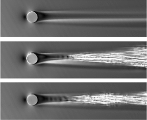
For configuration of case C, once a FST of  $Tu = 0.3\,\%$ is imposed at the inflow, the transition is triggered in the wake of the roughness similar to what is observed in case D. The flow structures are plotted in figure 14( $b$). It can be noticed that the wake of the roughness is a highly receptive flow region as mostly this area is affected by FST. This observation is consistent with the findings of Bucci et al. (Reference Bucci, Puckert, Andriano, Loiseau, Cherubini, Robinet and Rist2018) for a two-dimensional boundary-layer flow. The transition scenario in case C is significantly modified when a lower value of FST intensity ( $Tu=0.03\,\%$) is selected. This value corresponds to the natural level of FST in the MTL wind tunnel in which the experiments of Örlü et al. (Reference Örlü, Tillmark and Alfredsson2021) were performed. In figure 15, the isosurface of the spanwise velocity is reported for different time instants. As seen there, there is no fixed transition point behind the roughness, but some turbulent spots appear randomly. In the first snapshot, we can observe a large turbulent spot close to the outflow boundary and a smaller one in middle of the domain. In the other snapshots we can follow the evolution of the latter spot in time. While the developed turbulent spots leave the domain, new ones are generated which in turn propagate downstream. So, although such a low level of FST does not trigger the transition directly after the roughness, it can change the flow behaviour significantly.

Figure 15. Isosurface of instantaneous spanwise velocity  $w$ coloured by instantaneous chordwise velocity $u_\tau$ for case C and $Tu=0.03\,\%$ at different time (increasing time from (a) to (d)).
In figure 16, the instantaneous friction coefficient  $C_{f}$ is plotted for case C with $Tu=0.0\,\%$ and $0.3\,\%$ as well as case D with $Tu=0.0\,\%$. In the first case, we can recognize the footprint of the high- and low-speed streaks demonstrated as the region of the higher and lower $C_{f}$, respectively. In case C with $Tu=0.3\,\%$ and case D with $Tu=0.0\,\%$, first traces of some spanwise vortices are observed. Once transition takes place, a region of elongated chordwise structures with mainly higher values of $C_f$ appears and the turbulent region spreads in the spanwise direction as it propagates downstream.

Figure 16. Instantaneous friction coefficient for  $(a)$ case C, $(b)$ case D and $(c)$ case C ( $Tu=0.3\,\%$).
To further investigate the observed unsteady flows, we subtract the steady solution from the instantaneous flow fields and visualize the structures. The isosurfaces of negative and positive chordwise velocity  $u_\tau '$ are shown in figure 17. Again, this indicates that initially structures are concentrated around the low-speed streaks. In case D, some hairpin-like structures can be observed close to the roughness element which eventually break down into a more complex and chaotic flow pattern. The perturbation field close to the roughness element in case C does not exhibit structures as organizedas in case D. However, similar hairpin-like structures can still be recognized there. In order to understand if the fluctuations in these cases are dominated by similar structures, the time signal, the mean and the root-mean-square (r.m.s.) values in the transitional region are computed at $x=0.185$ and shown in figures 18 and 19. If the structures responsible for the transition are the same, the time signal should have a similar spectral content and the same should hold for the spatial support of the perturbations. In figure 18, the time signals and their power spectral density (PSD) for case C with $Tu=0.3\,\%$ and case D with $Tu=0.0\,\%$ are presented. As can be seen there, the perturbations in case C with $Tu=0.3\,\%$ are stronger (due to the forcing by FST) than in case D but they have a similar frequency content, as shown in figures 18 $(b)$ and 18 $(d)$. In case C the maximum of PSD is found for $f\approx 56$ and in case D for $f\approx 71$. These values, if scaled with the roughness height and the total velocity at the location of the roughness height, are $f_h=f^*h^*/Q^*(h^*)=0.076$ and 0.113, respectively. If instead the diameter of the roughness element is used as the reference length, the non-dimensional frequencies are $f_d=f^*d^*/Q^*(h^*)=1.5$ and 1.6, respectively. Further, case C presents relatively high fluctuations also for $10< f<30$ which are not present in case D. This may be due to the noise generated by FST. In figure 19, we can see that also the r.m.s. fields present similarities. In both cases the high r.m.s. values are located close to $z=0$ where also the highest values of $\partial u_{\tau } / \partial z$ were found (see figure 11). At this spanwise position, the mean value of the chordwise velocity is $\bar {u}_{\tau } \approx 0.7$.

Figure 17. Isosurface of negative (blue) and positive (red) instantaneous chordwise perturbation velocity  $u_\tau '$. Shaded pseudocolour represents friction coefficient. $(a)$ Case D and $(b)$ case C ( $Tu=0.3\,\%$).

Figure 18. Time signals  $(a{,}c)$ and PSD $(b{,}d)$ of the velocity fluctuations of $u_{\tau }$ around the mean value. Probe location is $(x,n,z)=(0.185, 0.001 , 0.0)$. $(a{,}b)$ Case D and $(c{,}d)$ case C with $Tu = 0.3\,\%$.

Figure 19. Mean value  $(a{,}c)$ and r.m.s. $(b{,}d)$ of $u_{\tau }$ at $x=0.185$. $(a{,}b)$ Case D and $(c{,}d)$ case C with $Tu = 0.3\,\%$.
4.2.2. Impulse–response analysis
In order to further study the stability characteristics of the flow behind the roughness elements, we performed an impulse–response analysis similar to the one carried out by Brandt et al. (Reference Brandt, Cossu, Chomaz, Huerre and Henningson2003), Peplinski, Schlatter & Henningson (Reference Peplinski, Schlatter and Henningson2015) and Brynjell-Rahkola et al. (Reference Brynjell-Rahkola, Shahriari, Schlatter, Hanifi and Henningson2017). We introduced a wave-packet disturbance, as in Bech, Henningson & Henkes (Reference Bech, Henningson and Henkes1998), upstream of the roughness element and monitored its evolution. This is done in a linear framework where the steady solutions discussed in previous sections are used as the base flow. In particular, we analyse evolution of the disturbance kinetic energy to obtain some insights about the linear behaviour of small perturbations.
In figure 20, the evolution of the total kinetic energy  $K_T$ (integrated in the whole domain) of the wave packet as a function of time is given for cases B, C, D and E. As can be seen there, in all cases $K_T$ decreases initially and then it starts growing for $t\approx 0.1$. With the exception of case D, $K_T$ decreases again for $t>0.2$. The evolution of the wave packet for case D is very different. While the energy of the wave packet in cases B, C and E exponentially decays after it has reached its maximum, in case D it grows exponentially continuously after an initial transient stage. This indicates that flow in case D may be globally unstable.

Figure 20. Time evolution of the energy of the wave packet. Blue line represents case B, red line case C, green line case D and black line case E.
In order to further analyse the response of the flow to the impulse, we monitor the disturbance kinetic energy of the wave packet  $K$ (integrated in the $n$–
$n$– $z$ plane) as a function of space and time. Results for cases C and D are presented in figure 21. The same analysis for cases B and E showed a similar behaviour of $K$. Figure 21( $a$) shows the evolution of $K$ as a function of chordwise coordinate $x$ for case C. The disturbance energy grows downstream until it reaches its maximum at some $x$ position and then decays. The location of this maximum moves downstream with increasing time. The maximum over time and space is reached for $t\approx 0.25$ and $x\approx 0.25$. As can be seen there, for $x \le 0.20$ the energy decreases in time suggesting that the wave packet does not stay in place but it travels downstream and it is eventually advected out of the domain. This indicates the convective character of the flow instability in case C. In case D a different behaviour is observed. As shown in figure 21( $b$), the disturbance energy, which is significantly larger than in case C, grows contentiously in time.

Figure 21. Energy in the wall-normal planes against the chordwise coordinate (a) for case C and (b) for case D, and (c) against the propagation velocity  $c_g$ for case D.
In the case where the flow is globally unstable, the wave packet will travel in both upstream and downstream directions, while if it is convectively unstable, disturbances will propagate downstream and eventually leave the computational domain. In the latter scenario, the velocity of the trailing edge of the wave packet will be positive, whereas in the case of global instability it will be negative (Schmid & Henningson Reference Schmid and Henningson2001). In order to find the propagation velocity of the wave packet, we plot  $K$ as a function of $c_g=(\tau -\tau _0)/t$, where $\tau _0$ is the tangential coordinate of a point just behind the roughness element. Figure 21( $c$) shows the disturbance energy $K$ as a function of $c_g$ for different time instants. We can observe that the rear part of the curves for $t > 0.15$ crosses at a negative value of $c_g$, which indicates that the wave packet travels upstream. Hence, this case appears to be globally unstable. This result is consistent with that of the nonlinear simulations where flow transitioned to turbulent in the absence of external disturbances ( $Tu=0.0\,\%$).
In figure 22, the wave packets for cases C and D at  $t=0.25$ are given showing the isosurfaces of negative and positive chordwise velocity. As seen there, in both cases the wave is located in the low-speed region behind the roughness element. In case C, the wave packet evolves forming elongated low- and high-speed regions inclined to the direction of the vortices created by the roughness element. In case D, the structure is almost perpendicular to the axis of the vortex with a shorter wavelength. One can see a similarity between these structures and those found in our nonlinear simulations illustrated in figure 17. These structures also bear similarities to the global modes found in the works of Kurz & Kloker (Reference Kurz and Kloker2016) (figure 27 therein) and Brynjell-Rahkola et al. (Reference Brynjell-Rahkola, Shahriari, Schlatter, Hanifi and Henningson2017) (figure 10 therein). The one observed in case C corresponds to the low- to moderate-frequency modes (of the $z$-mode type ) in those works, while the structure in case D is similar to the high-frequency global modes. The similarity to results of global mode analysis in the mentioned works is also confirmed by the results presented in figure 18, where the dominant frequencies in the flow are shown.

Figure 22. Isosurface of negative (blue) and positive (red) chordwise velocity of the wave packet for  $(a)$ case C and $(b)$ case D. Pseudocolour represents the friction coefficient at the wall.
4.2.3. Energy budget analysis
Here, we analyse the energy budget of the wave packet discussed above by computing the contributions from the production and dissipation terms of the Reynolds–Orr equations (Schmid & Henningson Reference Schmid and Henningson2001):
 \begin{equation} \frac{\partial K_T}{\partial t} ={-}D + \sum_{i=1}^{9} Pr_{i}, \end{equation}
where the dissipation term  $D$ is given by
 \begin{equation} \frac{1}{Re} \int_{\varOmega} \boldsymbol{u}' : \boldsymbol{u}' \, \textrm{d}\varOmega, \end{equation}
with  $\boldsymbol {u}'$ being the perturbation velocity.
The production terms are the following:
 \begin{equation} \left. \begin{aligned} Pr_1 ={-} \int_{\varOmega} u_{\tau}'^2 \frac{\partial u_{\tau}}{ \partial \tau} \, \textrm{d}\varOmega, \quad Pr_2 ={-} \int_{\varOmega} u_{\tau}'u_{\eta}' \frac{\partial u_{\tau}}{ \partial \eta} \, \textrm{d}\varOmega, \quad Pr_3 ={-} \int_{\varOmega} u_{\tau}'u_{z}' \frac{\partial u_{\tau}}{ \partial z} \, \textrm{d}\varOmega,\\ Pr_4 ={-} \int_{\varOmega} u_{\eta}'u_{\tau}' \frac{\partial u_{\eta}}{ \partial \tau} \, \textrm{d}\varOmega, \quad Pr_5 ={-} \int_{\varOmega} u_{\eta}'^2 \frac{\partial u_{\eta}}{ \partial \eta} \, \textrm{d}\varOmega, \quad Pr_6 ={-} \int_{\varOmega} u_{\eta}'u_{z}' \frac{\partial u_{\eta}}{ \partial z} \, \textrm{d}\varOmega,\\ Pr_7 ={-} \int_{\varOmega} u_{z}'u_{\tau}' \frac{\partial u_{z}}{ \partial \tau} \, \textrm{d}\varOmega, \quad Pr_8 ={-} \int_{\varOmega} u_{z}'u_{\eta}' \frac{\partial u_{z}}{ \partial \eta} \, \textrm{d}\varOmega, \quad Pr_9 ={-} \int_{\varOmega} u_{z}'^2 \frac{\partial u_{z}}{ \partial z} \, \textrm{d}\varOmega. \end{aligned} \right\} \end{equation}
Here,  $\{ u_{\tau },u_{\eta },u_{z} \}$ are the three velocity components of the stationary solution. In the case where the sum of the production terms is greater than the dissipation, the energy of the perturbation grows in time. The production terms can be either positive or negative causing destabilization or stabilization of the perturbations, respectively. In figure 23 $(a)$ we report the ratio between the total production and the dissipation for cases C and D. As seen there, in case D the ratio is always greater than one, apart from at the first instants, and thus we have a positive contribution to the growth of the perturbation. On the contrary, in case C we can see that the dissipation terms are greater than the sum of the production ones for $t>0.22$ and so the kinetic energy of the perturbation decreases. Up to that time, also in case C we can observe an initial growth of the perturbation which is in agreement with the study of a two-dimensional boundary layer performed by (Cherubini et al. Reference Cherubini, De Tullio, De Palma and Pascazio2013). These observations are consistent with the behaviour of $K_T$ shown in figure 20. For case D, the contribution from each term of (4.1), scaled with the value of the dissipation, is shown in figure 23. It is found that the term $Pr_3$ gives the largest contribution. This is in agreement with the observation of Loiseau et al. (Reference Loiseau, Robinet, Cherubini and Leriche2014) for the unstable varicose mode generated by a roughness element in a two-dimensional boundary layer. The main difference between their results and those presented in figure 23 is the significant contribution from the term $Pr_9$. This is due to the fact that here the spanwise velocity component of the base flow has values comparable to those of the chordwise one.

Figure 23.  $(a)$ Ratio between the sum of the production terms and the dissipation as a function of time for case C (red) and case D (green). $(b)$ Contribution to the energy budget of each production term $Pr_i$ scaled with the dissipation for case D.
5. Summary and conclusions
The flow over a swept wing in the presence of disc-type roughness elements has been investigated by means of DNS. The main goal of this study is to investigate the nature of the instability caused by the roughness elements with high aspect of ratio and their interaction with FST. Through our numerical simulations, we try to explain the behaviour of wake flow behind the roughness elements (the heat transfer investigated using infrared images) and its sensitivity to FST intensity observed in the experiments of Örlü et al. (Reference Örlü, Tillmark and Alfredsson2021). To do so, FST with the same intensity and integral length scale as in the experiments is imposed at the inflow.
Nonlinear simulations performed with zero FST showed that for roughness elements with different widths and a height up to 0.8 mm ( $h/\delta ^*=1.44$, $Re_{hh}=461$), flow behind the roughness was steady and no transition was observed. On the contrary, simulations for $h/\delta ^*=2.0$ ( $Re_{hh}=712$) showed a turbulent flow just behind the roughness element. In the experiments, with a FST level of $Tu=0.3\,\%$ transition was observed at the location of the roughness for $h/\delta ^*=1.44$ and $d/h=20$. Even at the lowest FST level ( $Tu=0.03\,\%$), a strong effect on transition was observed for this case. These observations were confirmed by our simulations when the same levels of FST were used.
The common feature of the flow behind the roughness elements, when non-transitional, is the existence of a series of high- and low-speed streaks formed due to the lift-up effect. Due to the presence of the cross-flow component of the base flow, the spanwise distribution of these streaks is not symmetric as in the case of a two-dimensional boundary layer. The rightmost high-speed streak, as well as the low-speed streaks next to it, grows in amplitude along the streamwise direction. The central low-speed streak on the contrary decays. Different from the observation of Kurz & Kloker (Reference Kurz and Kloker2016) and Brynjell-Rahkola et al. (Reference Brynjell-Rahkola, Shahriari, Schlatter, Hanifi and Henningson2017), the vortices generated behind the roughness elements did not merge here. This can be due to the wider roughness elements used in our studies. Moreover, we have observed that increasing the diameter does not cause a significant change in the stability of the flow.
The transition caused by large roughness elements is thought to be a result of the global instability of the flow generated by these elements (Loiseau et al. Reference Loiseau, Robinet, Cherubini and Leriche2014; Kurz & Kloker Reference Kurz and Kloker2016; Brynjell-Rahkola et al. Reference Brynjell-Rahkola, Shahriari, Schlatter, Hanifi and Henningson2017). Here, we have investigated the instability characteristics of the flow behind the roughness elements by means of an impulse–response analysis. For all cases with  $h/\delta ^*=1.44$, the wave packet generated by the impulse grows weakly downstream of the roughness until $x \approx 0.25$ and then decays and exits the computational domain. The scenario is very different for the case with $h/\delta ^*=2.0$, where the wave packet grows by several orders of magnitude and expands in the space behind the roughness. Further, the trailing edge of the generated wave packet has a negative propagation velocity meaning the flow is absolutely unstable in this case. The origin of the flow instability is found to be located in the low-speed flow region behind the roughness and creates hairpin-vortex-like structures which then rapidly break down. An energy budget analysis of case D showed, as expected, that the total contribution of the production terms is greater than the dissipation resulting in growth of the total kinetic energy. The terms associated with the spanwise gradient of the base flow are the ones giving the major contributions. On the contrary, in case C after the initial transient the dissipation is higher than production and so the perturbation is damped.
Although the impulse–response analysis for case C revealed a weak growth of the wave packet, a continuous forcing with a FST level of  $Tu = 0.3\,\%$ was found to be sufficient to trigger the flow transition behind the roughness element. This transition takes place in the low-speed region as in the unstable case, but the flow pattern appears to be more chaotic. A comparison between the time signals and their r.m.s. values retrieved in the transitional region showed that the fluctuations for case C with $Tu = 0.3\,\%$ and case D have a similar spectral content and spatial support. This suggests that in both cases those fluctuations may have been governed by similar instability modes. Outside the wake the flow does not appear to be significantly affected which indicates that the low-speed region is highly receptive to the forcing caused by the FST. We also have found that for $Tu=0.03\,\%$ flow exhibits travelling turbulent spots which randomly appear due to the convectively unstable disturbances. These observations were found to be consistent with experimental findings (Örlü et al. Reference Örlü, Tillmark and Alfredsson2021) where for $h/\delta ^*=1.44$ and $d/h=20$ with $Tu =0.3\,\%$ a clear transition was observed, while for $Tu=0.03\,\%$ a strong effect was found but not a clear transition. Our analysis confirmed a large impact of FST level on the flow behaviour behind the subcritical roughness elements. A similar conclusion was drawn in Bucci et al. (Reference Bucci, Puckert, Andriano, Loiseau, Cherubini, Robinet and Rist2018) and Bucci (Reference Bucci2017) for the case of a two-dimensional boundary layer.
Acknowledgements
The authors wish to thank Dr Örlü for his helpful discussions concerning the experiments.
Funding
Financial support for this work was provided by the European Research Council under grant agreement 694452-TRANSEP-ERC-2015-AdG. The computations were performed on resources of the Swedish National Infrastructure for Computing (SNIC) at the PDC Center for High Performance Computing at the Royal Institute of Technology (KTH).
Declaration of interests
The authors report no conflict of interest.
Appendix A. Convergence study
In this appendix we present some results of our convergence studies by showing the influence of the polynomial order on the steady-state solutions and on the evolution of the wave packets.
Figure 24 shows contours of the chordwise perturbation velocity in the wall-normal plane for the polynomial orders  $N_p=7$ (black lines) and $N_p=11$ (white lines). As can be seen, there is a good agreement between these two solutions. We performed also a convergence test for the linear impulse–response analysis which is reported in figure 25. Also in this case a close agreement is found. In this work the simulations where run using the polynomial order $N_p = 11$.

Figure 24. Pseudocolour of chordwise velocity  $u_{\tau }$ in the $n$–
$n$– $z$ plane at $x=0.2$ ( $a$) and $x=0.4$ ( $b$). Black contour lines represent the solution for $N_p=7$ and white for $N_p=11$.

Figure 25. Energy in wall-normal planes against streamwise coordinate. Circles represent the solution with  $N_p = 7$, solid lines that with $N_p=11$.
Appendix B. BoostConv algorithm
This algorithm is inspired by Krylov-subspace methods and is able to both stabilize and accelerate the convergence of a dynamical system to a steady solution. The method is based on a least-squares minimization of the residual of an iterative procedure. Here, we briefly describe the basic idea of the algorithm. For further details, readers are referred to Citro et al. (Reference Citro, Luchini, Giannetti and Auteri2017) who also applied the method to stabilize the flow behind a hemispherical roughness element in a two-dimensional boundary layer. Let us consider the linear system
 \begin{equation} \boldsymbol{A} \boldsymbol{x}= \boldsymbol{b}. \end{equation}
If we apply an iterative method to compute the solution, we can write
 \begin{equation} \boldsymbol{x}_{n+1}=\boldsymbol{x}_{n} + \boldsymbol{B} \boldsymbol{r}_n, \end{equation}
where  $\boldsymbol {r}_n= \boldsymbol {b} - \boldsymbol {A} \boldsymbol {x}$ is the residual at step $n$ and $\boldsymbol {B}$ the matrix that describes the iterative procedure. Then, (B2) can be rewritten as
 \begin{equation} \boldsymbol{x}_{x+1} = \left ( \boldsymbol{I} - \boldsymbol{BA} \right ) \boldsymbol{x}_n + \boldsymbol{Bb}. \end{equation}
The convergence of the iterative procedure depends on the spectrum of the matrix  $( \boldsymbol {I} - \boldsymbol {BA})$. Often, the convergence is dictated only by a small part of the spectrum, either the least damped or the most amplified eigenvalues, depending on the system being stable or unstable, respectively. The algorithm aims to modify this part of the spectrum. Now, we consider the evolution equation for the residual:
 \begin{equation} \boldsymbol{r}_{n+1}=\boldsymbol{r}_{n} - \boldsymbol{ABr}_n, \end{equation}
which can be obtained from (B2) applying  $-\boldsymbol {A}$ and adding $\boldsymbol {b}$ on both sides. The central idea is to replace the residual $\boldsymbol {r}_n$ with a new one $\boldsymbol {\xi }_n(\boldsymbol {r}_n)$. We need to choose $\boldsymbol {\xi }_n$ such that $\boldsymbol {\xi }_n \rightarrow 0$ only when $\boldsymbol {r}_n \rightarrow 0$. If we substitute $\boldsymbol {r}_n$, equation (B4) reads
 \begin{equation} \boldsymbol{r}_{n+1}=\boldsymbol{r}_{n} - \boldsymbol{AB} \boldsymbol{\xi}_n (\boldsymbol{r}_n) . \end{equation}
Now, the task is to to choose  $\boldsymbol {\xi }_n$ such that $\boldsymbol {r}_{n+1}$ is minimized. To do so, a least-squares method is adopted to approximate the solution of $\boldsymbol {AB} \boldsymbol {\xi }_n =\boldsymbol {r}_{n}$. The value of $\boldsymbol {\xi }_n$ is approximated using the subspace of $\boldsymbol {AB}$ built through its repeated action. It should be noticed that the described procedure requires only the knowledge of the residuals $\boldsymbol {r}_n$ to compute $\boldsymbol {\xi _n}$ and for that reason can be included as a black box in the original procedure.


 Open access