


1. Introduction
Thermal convection refers to fluid flows that are driven by buoyancy forces due to density variations, which in turn are caused by gradients in temperature (Chandrasekhar Reference Chandrasekhar2013). Such flows are ubiquitous in both the natural and engineering environments, and are key to understanding transport phenomena in the atmospheric boundary layer, in the outer core of Earth and in the outer layers of stars (Kadanoff Reference Kadanoff2001; Wettlaufer Reference Wettlaufer2011) to name a few examples. The simplest setting in which thermal convection can be studied is classical Rayleigh–Bénard convection (RBC) in which a fluid is confined between two flat horizontal plates with the under side maintained at a higher temperature than the top (Rayleigh Reference Rayleigh1916). Applying the Boussinesq approximation to the Navier–Stokes equations, the dynamics of RBC is governed by three non-dimensional parameters: the Rayleigh number  $Ra$, the ratio of buoyancy to viscous forces, the Prandtl number $Pr$, the ratio of the fluid's kinematic viscosity to its thermal diffusivity, and the aspect ratio $\varGamma$ of the flow domain.
Heat transport in a fluid at rest is due solely to thermal conduction and when convective motions ensue this transport is enhanced. The Nusselt number  $Nu$, the ratio of total heat flux to conductive heat flux, is the quantitative measure of this enhancement. Determining the dependence of $Nu$ on $Ra$,
$Ra$,  $Pr$ and $\varGamma$ for asymptotically large values of $Ra$ has been a major goal of the studies of convection; see, e.g. Spiegel (Reference Spiegel1971), Kadanoff (Reference Kadanoff2001), Ahlers, Grossmann & Lohse (Reference Ahlers, Grossmann and Lohse2009), Chillà & Schumacher (Reference Chillà and Schumacher2012) and references therein. Specifically, if $Nu$ is sought in terms of a power law $Nu = A(Pr, \varGamma )Ra^{\beta }$ then the goal is to determine the value of the exponent $\beta$ for $Ra \gg 1$.
For planar geometries, if one assumes that the dimensional heat flux becomes independent of the depth of the cell as  $Ra \rightarrow \infty$, then one obtains $Nu \sim Ra^{1/3}$. This is the so-called classical theory of Priestley (Reference Priestley1954), Malkus (Reference Malkus1954) and Howard (Reference Howard1966). However, if one assumes that the dimensional heat flux becomes independent of the molecular properties of the fluid when $Ra \rightarrow \infty$, then one obtains $Nu \sim (Pr \, Ra)^{1/2}$. This ‘mixing length’ theory is originally due to Spiegel (Reference Spiegel1963) and such scaling behaviour – with possible logarithmic corrections (Kraichnan Reference Kraichnan1962; Chavanne et al. Reference Chavanne, Chilla, Castaing, Hebral, Chabaud and Chaussy1997) – is now often referred to as the ultimate regime of thermal convection. The scaling $Nu \sim Ra^{1/2}$ is also an upper limit (uniformly in $Pr$) to the asymptotic heat transport scaling as $Ra \rightarrow \infty$ for no-slip fixed-temperature boundaries whether they are flat (Howard Reference Howard1963; Doering & Constantin Reference Doering and Constantin1996) or corrugated, i.e. textured but sufficiently smooth (Goluskin & Doering Reference Goluskin and Doering2016). (For flat no-slip boundaries at infinite Prandtl number the best known upper bound corresponds to the classical scaling $Nu \lesssim Ra^{1/3}$ within logarithmic corrections (Constantin & Doering Reference Constantin and Doering1999; Doering, Otto & Reznikoff Reference Doering, Otto and Reznikoff2006; Otto & Seis Reference Otto and Seis2011). In a wide range of studies at ${O}(1)$ Prandtl number, the exponent $\beta$ is found to vary between $2/7$ (Verzicco & Camussi Reference Verzicco and Camussi2003; Johnston & Doering Reference Johnston and Doering2009; Stevens, Verzicco & Lohse Reference Stevens, Verzicco and Lohse2010; Urban, Musilová & Skrbek Reference Urban, Musilová and Skrbek2011; Urban et al. Reference Urban, Hanzelka, Kralik, Musilova, Srnka and Skrbek2012; Doering, Toppaladoddi & Wettlaufer Reference Doering, Toppaladoddi and Wettlaufer2019; Iyer et al. Reference Iyer, Scheel, Schumacher and Sreenivasan2020) and $1/3$ (Niemela et al. Reference Niemela, Skrbek, Sreenivasan and Donnelly2000; Niemela & Sreenivasan Reference Niemela and Sreenivasan2003; Verzicco & Camussi Reference Verzicco and Camussi2003; Niemela & Sreenivasan Reference Niemela and Sreenivasan2006; Stevens et al. Reference Stevens, Verzicco and Lohse2010; Urban et al. Reference Urban, Musilová and Skrbek2011, Reference Urban, Hanzelka, Kralik, Musilova, Srnka and Skrbek2012; Doering et al. Reference Doering, Toppaladoddi and Wettlaufer2019; Iyer et al. Reference Iyer, Scheel, Schumacher and Sreenivasan2020). Several experiments have reported $\beta > 1/3$ (Chavanne et al. Reference Chavanne, Chilla, Castaing, Hebral, Chabaud and Chaussy1997; He et al. Reference He, Funfschilling, Nobach, Bodenschatz and Ahlers2012); however, because of the diversity of scalings reported for overlapping ranges of $Ra$, those findings await independent confirmation (Urban et al. Reference Urban, Hanzelka, Kralik, Musilova, Srnka and Skrbek2012; He et al. Reference He, Funfschilling, Nobach, Bodenschatz and Ahlers2013; Urban et al. Reference Urban, Hanzelka, Kralik, Musilova, Srnka and Skrbek2013; Skrbek & Urban Reference Skrbek and Urban2015; He, Bodenschatz & Ahlers Reference He, Bodenschatz and Ahlers2016).
The key difference between the classical ( $\beta = 1/3$) and the ultimate ( $\beta = 1/2$) theories principally lies in the role played by the thermal boundary layers. In the former regime, thermal boundary layers presumably limit the rate of transport and hence control it (Howard Reference Howard1966). In the latter regime, the transport of heat is predominantly due to convective motions (Kraichnan Reference Kraichnan1962; Spiegel Reference Spiegel1963). Indeed, these regimes have been observed in recent experiments on radiatively driven convection (Lepot, Aumaître & Gallet Reference Lepot, Aumaître and Gallet2018; Bouillaut et al. Reference Bouillaut, Lepot, Aumaître and Gallet2019). Hence, it is necessary to investigate the role of thermal boundary layers in turbulent convection to determine the asymptotic high Rayleigh number heat transport.
Motivated by the studies that used surface roughness to probe the boundary layers in turbulent shear flows, Shen, Tong & Xia (Reference Shen, Tong and Xia1996) studied turbulent thermal convection experimentally in a cell whose top and bottom surfaces were covered with pyramidal roughness elements of aspect ratio  $2$, where the aspect ratio is the element width to height. They observed that roughness led to the emission of a larger number of plumes compared to that in convection over smooth surfaces, and that when $Ra$ was above a certain threshold, $Nu$ increased by $20\,\%$ compared to its value for smooth surfaces. However, the value of $\beta \approx 2/7$ was found to be the same as that for planar surfaces for the range of $Ra$ considered. In later experiments, Du & Tong (Reference Du and Tong1998, Reference Du and Tong2000) concluded similarly. Several subsequent studies, however, report that roughness does lead to an increase in $\beta$ from its planar value (Roche et al. Reference Roche, Castaing, Chabaud and Hébral2001; Qiu, Xia & Tong Reference Qiu, Xia and Tong2005; Stringano, Pascazio & Verzicco Reference Stringano, Pascazio and Verzicco2006; Tisserand et al. Reference Tisserand, Creyssels, Gasteuil, Pabiou, Gibert, Castaing and Chilla2011; Salort et al. Reference Salort, Liot, Rusaouen, Seychelles, Tisserand, Creyssels, Castaing and Chilla2014; Wei et al. Reference Wei, Chan, Ni, Zhao and Xia2014; Toppaladoddi, Succi & Wettlaufer Reference Toppaladoddi, Succi and Wettlaufer2015a; Wagner & Shishkina Reference Wagner and Shishkina2015; Toppaladoddi, Succi & Wettlaufer Reference Toppaladoddi, Succi and Wettlaufer2017; Zhu et al. Reference Zhu, Stevens, Verzicco and Lohse2017).
The first study to use roughness to manipulate the interaction between the boundary layers and the outer region to attain the ultimate regime was that of Roche et al. (Reference Roche, Castaing, Chabaud and Hébral2001) who studied convection experimentally in a cylindrical cell covered by V-shaped grooves on all sides. They observed that when the thickness of the thermal boundary layers becomes smaller than the amplitude of roughness,  $\beta$ attains a value of $0.51$ for $Ra = [2 \times 10^{12}, 5 \times 10^{13}]$. Later, Toppaladoddi et al. (Reference Toppaladoddi, Succi and Wettlaufer2015a, Reference Toppaladoddi, Succi and Wettlaufer2017) used DNS in two dimensions to systematically manipulate this interaction by varying the wavelength of sinusoidal upper and/or lower surfaces at a fixed amplitude. They discovered the existence of an optimal wavelength at which $\beta$ is maximized, and that for wavelengths much smaller and much greater than the optimal wavelength $\beta$ attains its planar value. They also found that $\beta = 0.483$ for the optimal wavelength when both top and bottom surfaces are corrugated (Toppaladoddi et al. Reference Toppaladoddi, Succi and Wettlaufer2017). Their findings that roughness wavelength modulation leads to optimal heat transport and results in $\beta \approx 0.5$ for a certain wavelength were subsequently confirmed by experimental (Xie & Xia Reference Xie and Xia2017) and numerical (Zhu et al. Reference Zhu, Stevens, Verzicco and Lohse2017) studies, although it has been suggested that $\beta$ can decrease again at even higher $Ra$ (Zhu et al. Reference Zhu, Stevens, Verzicco and Lohse2017). More recently, Zhu et al. (Reference Zhu, Stevens, Shishkina, Verzicco and Lohse2019) reported $Nu \sim Ra^{1/2}$ for $Ra = [10^8, 10^{11}]$ over corrugated surfaces with just three characteristic length scales.
The central physical issue we are addressing here is as follows. As emphasized above, the regimes of determining the exponent  $\beta$ centre around the interaction of the thermal boundary layers and the core flow. As the Rayleigh number increases the thermal boundary layers thin. Indeed, as first noted by Niemela & Sreenivasan (Reference Niemela and Sreenivasan2006), one can understand the results of Roche et al. (Reference Roche, Castaing, Chabaud and Hébral2001) as a transition between a regime where the groove depth is less than the thermal boundary-layer thickness to a regime where the groove depth is larger than the boundary thickness. Thus, as emphasized by Toppaladoddi et al. (Reference Toppaladoddi, Succi and Wettlaufer2017), when a given experiment or simulation has a fixed roughness geometry, the boundary-layer core flow interaction may evolve as the Rayleigh number increases. It is for this reason that surfaces with a spectrum of roughness length scales are of interest.
Although we have considerable understanding of the effects of periodic corrugation on plume production and heat transport, it is still not clear a priori if these results can be used to describe the effects of fractal roughness. Indeed, there have been far fewer studies on turbulent convection over multi-scale surfaces, the earliest being that of Villermaux (Reference Villermaux1998) who theoretically considered the effects of fractal surfaces with power-law distributed amplitudes. Villermaux (Reference Villermaux1998) argued that given a regime where  $Nu \sim Ra^{2/7}$ for smooth boundaries, the effective exponent increased from $2/7$ to $1/3$ with increasing degree of roughness. Ciliberto & Laroche (Reference Ciliberto and Laroche1999) studied the effects of power-law distributed fractal surfaces on the heat transport experimentally and found larger $\beta$ values of $0.35$ and $0.45$ depending on the distribution of roughness amplitudes. Those studies motivate our own.
In this work we consider the effects of one fractal boundary on the dynamics and bulk transport properties of turbulent Rayleigh–Bénard convection and address the following questions: (i) What are the effects of fractal surface roughness on the heat transport? (ii) How sensitive is the heat transport to the details of the roughness realization? (iii) Can one infer the characteristic length scale(s) of roughness from a study of its effects on the flow? We do this using well resolved two-dimensional (2-D) numerical simulations using the lattice Boltzmann method. The choice of the domain and roughness properties is motivated by our aim to understand the interactions between rough Arctic sea ice and the underlying ocean.
2. Governing equations
The spatial domain in our study (in dimensional units) is  $(x,z) \in [0,L]\times [0,h(x)]$ where $0 < h(x) \le H$ is the vertical height of the layer at horizontal position $x$. We model thermal convection via the Oberbeck–Boussinesq equations (Rayleigh Reference Rayleigh1916; Chandrasekhar Reference Chandrasekhar2013), non-dimensionalizing the system using the length scale $H$, the free-fall velocity scale $u_0 = \sqrt {g \alpha {\rm \Delta} T H}$, where $g$ is acceleration of gravity, $\alpha$ is the coefficient of thermal expansion, ${\rm \Delta} T$ is the temperature difference between the bottom and top boundaries and the free-fall time scale $t_0 = H/u_0$.
The equations and boundary conditions for the dimensionless velocity, temperature and pressure fields,  $\boldsymbol {u}(\boldsymbol {x},t) = [u(\boldsymbol {x},t), w(\boldsymbol {x},t)]$, $T(\boldsymbol {x},t)$ and $p(\boldsymbol {x},t)$, are
 \begin{gather} \boldsymbol{\nabla} \boldsymbol{\cdot} \boldsymbol{u} = 0, \end{gather}
 \begin{gather}\frac{\partial \boldsymbol{u}}{\partial t} + \boldsymbol{u} \boldsymbol{\cdot} \boldsymbol{\nabla} \boldsymbol{u} = -\boldsymbol{\nabla} p + T \boldsymbol{k} + \sqrt{\frac{Pr}{Ra}} \nabla^2 \boldsymbol{u}, \end{gather}
 \begin{gather}\frac{\partial T}{\partial t} + \boldsymbol{u} \boldsymbol{\cdot} \boldsymbol{\nabla} T = \sqrt{\frac{1}{Ra \, Pr}} \nabla^2 T, \end{gather}
 \begin{gather}\boldsymbol{u} = 0 \quad \text{and} \quad T = 1 \quad \text{at}\ z = 0, \end{gather}
 \begin{gather}\boldsymbol{u} = 0 \quad \text{and} \quad T = 0 \quad \text{at}\ z = h(x). \end{gather}
The Rayleigh number is  $Ra = \alpha g {\rm \Delta} T H^3/\kappa \nu$, where $\nu$ is the kinematic viscosity and $\kappa$ is the thermal diffusivity of the fluid, and the Prandtl number is $Pr = \nu /\kappa$. The fractal boundaries are such that $0.9 \le h(x) \le 1$. All variables are periodic in the horizontal $x$ direction, and the aspect ratio of the domain is $\varGamma = L/H$.
The bulk heat transport is measured by the Nusselt number,
 \begin{equation} Nu = \frac{\left\langle\overline{w^* T^*}\right\rangle - \kappa \left\langle\dfrac{\partial \bar{T}^*}{\partial z^*}\right\rangle}{\kappa {\rm \Delta} T/H}, \end{equation}
evaluated across horizontal layers in the cell. Here, the superscript  $*$ indicates the variable is dimensional, and $\overline {(\cdot )}$ and $\left \langle \cdot \right \rangle$ indicate horizontal and time averages, respectively. We compute $Nu$ at eight different heights in the cell and report the average value over these locations.
We use the lattice Boltzmann method (Benzi, Succi & Vergassola Reference Benzi, Succi and Vergassola1992; Chen & Doolen Reference Chen and Doolen1998; Succi Reference Succi2001) to solve the governing equations numerically. The principal reason for this choice of numerical method is the ease with which one can impose the boundary conditions for the velocity and temperature fields on complicated domains (Succi Reference Succi2001). The code used here has been tested extensively in Toppaladoddi, Succi & Wettlaufer (Reference Toppaladoddi, Succi and Wettlaufer2015b) for different fluid flow problems (Clever & Busse Reference Clever and Busse1974; Lipps Reference Lipps1976; Rozhdestvensky & Simakin Reference Rozhdestvensky and Simakin1984) and was previously used to study turbulent convection over planar and corrugated (i.e. smooth but non-flat) upper and lower boundaries (Toppaladoddi et al. Reference Toppaladoddi, Succi and Wettlaufer2015a, Reference Toppaladoddi, Succi and Wettlaufer2017).
We performed extensive checks on spatio-temporal convergence with the fractal boundaries used in the study. The spatial resolutions used in our simulations were such that the Kolmogorov length scale was resolved with at least two grid points everywhere in the domain (see table 1) and the boundary layer was resolved with at least eight grid points (see table 2). The simulations were run for sufficiently long times to attain a stationary state and the statistics were collected over the last  $200$ time units, except for the $Ra = 10^{10}$ cases where the statistics were collected over the last $100$ time units. Details of these tests are provided in appendix A.
We should note here that the depth of the cell  $H$ is one of the many choices for the characteristic length scale for this geometry. However, this choice only affects the pre-factor in power-law scalings for Nusselt and Reynolds numbers with Rayleigh number, and not the exponent. (See appendix B.)
3. Roughness profiles
Following Rothrock & Thorndike (Reference Rothrock and Thorndike1980), we consider upper boundary functions  $h(x)$ to be ‘rough’ when they are continuous but not differentiable. The increments in $h(x)$ are given by the Hölder condition,
 \begin{equation} \lim_{{\rm \Delta} x \to 0} \frac{\left|h(x+ {\rm \Delta} x) - h(x)\right|}{({\rm \Delta} x)^{\gamma}} = C, \end{equation}
where  $C$ is an ${O}(1)$ constant and $0 < \gamma \le 1$ is the Hölder exponent. Functions are Lipschitz continuous with a bounded derivative only when $\gamma = 1$. The power spectral density (PSD) of $h(x)$ for all non-zero wavenumbers $k$ decays as $\sim k^{p}$, where $p = -2 \gamma - 1$ (Rothrock & Thorndike Reference Rothrock and Thorndike1980). This characteristic decay of the PSD is a common feature shared by many natural and artificial surfaces, and thus can be used to classify different classes of rough surfaces (Sayles & Thomas Reference Sayles and Thomas1978; Rothrock & Thorndike Reference Rothrock and Thorndike1980).
To generate roughness profiles for the upper surface with the desired spectral properties for our simulations, we use the truncated Steinhaus series (Rothrock & Thorndike Reference Rothrock and Thorndike1980):
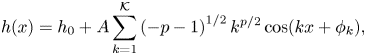 \begin{equation} h(x) = h_0 + A \sum_{k=1}^{\mathcal{K}} \left(-p-1\right)^{1/2} k^{p/2} \cos(k x + \phi_k), \end{equation}
where  $\mathcal {K}$ is the maximum wavenumber and $\phi _k$ are independent random variables uniformly distributed in $[0, 2{\rm \pi} ]$. It is clear that the PSD of $h(x)$ in (3.2) scales as $\sim k^p$ up to the cutoff wavenumber $\mathcal {K}$.
Figure 1 shows roughness functions for different values of  $p$ generated using (3.2). As $p$ is increased from $-3.0$ to $-1.5$, $h(x)$ becomes rough on smaller scales. It is also intuitively clear from figure 1 that with increasing roughness, as $\mathcal {K} \rightarrow \infty$, $h(x)$ tends to be more space filling than a 1-D curve but less space filling than a 2-D surface. Hence these curves are fractals in the limit $\mathcal {K} \rightarrow \infty$, with fractal or Hausdorff dimension $D_f = 2 - \gamma$ (Rothrock & Thorndike Reference Rothrock and Thorndike1980).We use (3.2) to generate the rough upper surfaces $h(x)$ for the simulations. All the rough surfaces used in this study have $\mathcal {K} = 100$ and the values of $h_0$ and $A$ are chosen such that their maximum and minimum amplitudes, measured from the top of the cell, are $0\,\%$ and $10\,\%$ of the depth of the cell, respectively. This implies that the upper portion of the fractal boundary coincides with the top flat surface. (See figure 2.)
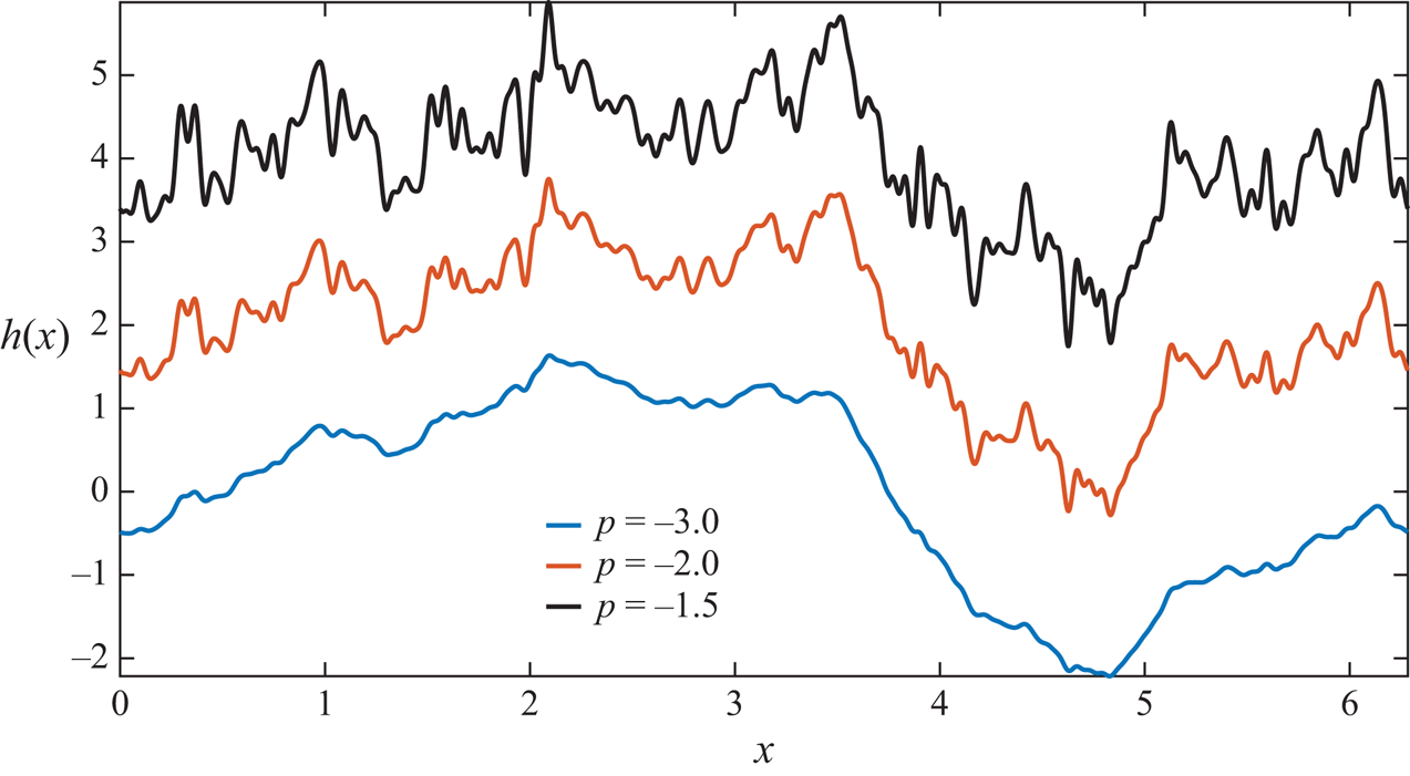
Figure 1. Functions used for the upper surface of the convecting domain generated using (3.2) for different values of  $p$ and for $\mathcal {K} = 100$. The degree of roughness increases as the value of $p$ increases. The curves are vertically displaced by $2$ units to improve their visibility.
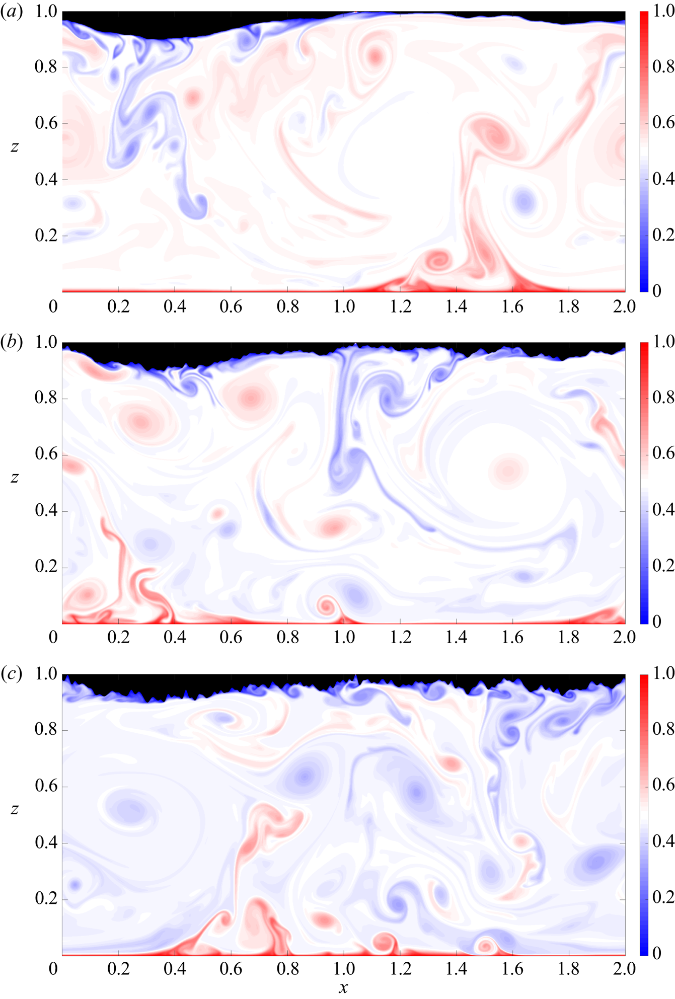
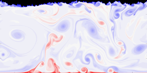
Figure 2. Temperature fields at  $t = 100$ for $Ra = 2.15 \times 10^9$ and (a) $p = -3.0$, (b) $p = -2.0$ and (c) $p = -1.5$. (See also the movies in the supplementary material available at https://doi.org/10.1017/jfm.2020.826.)
From figure 1 it is clear that there is a distribution of amplitudes associated with the fractal curves; hence, it is not a priori clear what choice of the characteristic length scale would be appropriate. The length scale chosen in our study is the depth of the cell  $H$. We present a detailed discussion of this point in appendix B, where we also show that a different choice of length scale simply leads to a uniform rescaling of $Nu$ and $Ra$ values for any given topography.
4. Results
The simulation results are for  $Pr = 1$ and $\varGamma = 2$. The simulations, except for $Ra = 10^{10}$, ran to at least $t = 330$ to allow adequate spin up, and in all cases the statistics were obtained for the last $200$ time units. The simulations for $Ra = 10^{10}$ were run for at least $t = 180$, and the statistics were collected over the last $100$ time units. See appendix A for details.
4.1. Temperature fields
Figure 2(a–c) shows the snapshots of the temperature fields for  $Ra = 2.15 \times 10^9$ and $p = -3, -2$ and $-1.5$, respectively. Focusing on the region close to the rough upper surfaces, for $p = -3$ (which is comparatively smooth) plumes are emitted only from a fraction of the surface and the temperature field is qualitatively similar to that for convection over flat walls (e.g. Johnston & Doering Reference Johnston and Doering2009). As seen in figures 2(b) and 2(c), however, as $p$ increases so too do the number of roughness elements triggering more plume generation: roughness enhances the coupling between the boundary layer and the core flow. Moreover, as seen in the case of a periodically corrugated upper surface (Toppaladoddi et al. Reference Toppaladoddi, Succi and Wettlaufer2015a), the enhanced emission of cold plumes decreases the mean interior temperature relative to the planar surface case.
4.2. Variation of heat flux with roughness properties
The  $Nu(Ra)$ data are shown in figure 3(a–c) for $Ra \in [10^7, 10^{10}]$ and (a) $p = -3.0$, (b) $p = -2.0$ and (c) $p = -1.5$, respectively. In these figures, for a given value of $p$, the simulations for the whole $Ra$ range were performed using the same realization of the fractal boundary. The scaling fits (i.e. linear least squares of the logarithms) are for $Ra \in [10^8, 10^{10}]$ and are shown as dashed lines in these figures. When $p$ increases from $-3.0$ to $-1.5$, the scaling exponent increases from $\beta = 0.288$ to $\beta = 0.352$. The power-law fit to the $Nu(Ra)$ data for $p=-3.0$ gives $Nu = 0.125 \times Ra^{0.288 \pm 0.005}$, which is remarkably close to $Nu = 0.138 \times Ra^{0.285}$ obtained for a similar $Ra$ range for flat boundaries in two dimensions (Johnston & Doering Reference Johnston and Doering2009). This suggests that, for this range of $Ra$, the fractal boundary corresponding to $p=-3.0$ is hydrodynamically smooth with respect to heat transport, even though it lies at the border between smooth and rough boundaries (Rothrock & Thorndike Reference Rothrock and Thorndike1980). For $p = -2.0$, the power-law fit gives $Nu = 0.055 \times Ra^{0.329 \pm 0.006}$, which is surprisingly close to $Nu = (0.0525 \pm 0.006) \times Ra^{0.331 \pm 0.002}$ obtained for $Ra \in [10^{10}, 10^{15}]$ for flat boundaries in a slender cylinder with $\varGamma = 0.1$ (Iyer et al. Reference Iyer, Scheel, Schumacher and Sreenivasan2020). And, lastly, for $p = -1.5$ the power law is $Nu = 0.037 \times Ra^{0.352 \pm 0.011}$, which is remarkably close to $Nu = 0.034 \times Ra^{0.359}$ obtained for (scaled) wavelength, $\lambda = 0.154$ for a sinusoidally corrugated boundary in two dimensions over $Ra \in [4 \times 10^6, 2.5 \times 10^9]$ (Toppaladoddi et al. Reference Toppaladoddi, Succi and Wettlaufer2015a). In fact, Toppaladoddi et al. (Reference Toppaladoddi, Succi and Wettlaufer2015a) found that $\lambda = 0.154$ was the optimal wavelength that maximized heat transport for their geometry. Evidently, heat transport increases with increasing degree of roughness, i.e. with $p$. This is in qualitative agreement with the results of Villermaux (Reference Villermaux1998), who also found that the scaling exponent increases with increasing roughness. However, the increase in $\beta$ is due to a change in the dynamics brought about by the introduction of surface roughness, principally the increase in plume production (Stringano et al. Reference Stringano, Pascazio and Verzicco2006; Toppaladoddi et al. Reference Toppaladoddi, Succi and Wettlaufer2015a, Reference Toppaladoddi, Succi and Wettlaufer2017), and not due to increased surface area. See appendix C for details. We also note that the power-law fits to the whole range of $Ra$ give: (a) $p = -3.0$: $Nu = 0.197 \times Ra^{0.267 \pm 0.015}$; (b) $p = -2.0$: $Nu = 0.111 \times Ra^{0.30 \pm 0.02}$; and (c) $p = -1.5$: $Nu = 0.069 \times Ra^{0.321 \pm 0.023}$.

Figure 3. Plots of  $Nu(Ra)$ versus $Ra \in [10^7, 10^{10}]$ for (a) $p = -3.0$, (b) $p = -2.0$ and (c) $p = -1.5$. Circles denote data from simulations and the dashed lines are the linear least-squares fits of $\log Nu$ to $\log Ra$ over the range $Ra \in [10^8, 10^{10}]$. The power laws are fit for the range $Ra \in [10^8, 10^{10}]$. For (a) $p=-3.0$, $Nu = 0.125 \times Ra^{0.288 \pm 0.005}$; (b) $p = -2.0$, $Nu = 0.055 \times Ra^{0.329 \pm 0.006}$; and (c) $p = -1.5$, $Nu = 0.037 \times Ra^{0.352 \pm 0.011}$. The error bar on each $Nu$ data point represents the standard deviation of the averaged $Nu$ calculated from eight different horizontal sections, and the uncertainties in $\beta$ are the $95\,\%$ confidence intervals.
The goodness of power-law fits can be tested by computing the residuals of the actual data from the fit data and examining them for any systematic curvature. These are shown in figure 4. It is apparent that the residuals do not exhibit any curvature for  $Ra \in [10^8, 10^{10}]$; hence, it can be concluded that the power laws describe the data well and more general fits are not required.
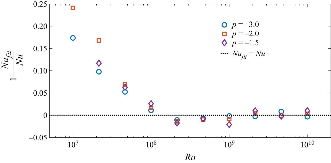
Figure 4. Residuals of the power-law fits shown in figure 3 for  $p = -3.0, -2.0$ and $-1.5$. Here, $Nu_{fit}$ are the values of the Nusselt number obtained from the power-law fits for the range $Ra \in [10^8, 10^{10}]$.
We can estimate an effective hydrodynamic length scale for the roughness amplitude by examining where the  $Nu(Ra)$ curves for different values of $p$ intersect. When boundary variations are present, the flow is not influenced by the roughness until the boundary layers become smaller than the amplitude of roughness (Roche et al. Reference Roche, Castaing, Chabaud and Hébral2001). Once this is achieved, as $Ra$ increases further the direct effects of roughness are associated with the increased number of plumes produced and the concomitant augmentation in $Nu$ (Roche et al. Reference Roche, Castaing, Chabaud and Hébral2001). We use similar ideas to estimate the effective roughness of the fractal boundaries. As seen in figures 1–3, the additional roughness structure introduced as $p$ is increased is associated with the increase in $\beta$. If one takes the $Nu-Ra$ curve for $p = -3$ as the benchmark case, then the intersection of this curve with that for a larger value of $p$ gives the value of the effective amplitude at which the transition to enhanced heat transport occurs. The choice of this reference is because $p=-3$ corresponds to $\gamma = 1$, representing the border between ‘smooth’ and ‘rough’ surfaces (Rothrock & Thorndike Reference Rothrock and Thorndike1980). Thus the effects of any additional roughness (see figure 1) can be conveniently studied with respect to the surface for $p=-3$. This transition happens at $Ra \approx 2.15 \times 10^8$, and the value of $Nu$ at this point is $\approx 31$ (see the $Nu$ values for the fourth realizations ( $r = 4$) in tables 3–5). Hence, the transition occurs when the effective amplitude of roughness $h_f$ over the surfaces with $p = -2$ and $p = -1.5$ first exceeds the boundary layer thickness $\delta _T$ for the curve with $p = -3$, so that the roughness elements protrude outside of the boundary layer and interact with the interior of the flow. Using the planar-wall estimate of $Nu$, we estimate the cross-over scaling as
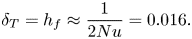 \begin{equation} \delta_T = h_f \approx \frac{1}{2 Nu} = 0.016. \end{equation}
Thus, the effective amplitude of the roughness for surfaces with  $p=-2$ and $p=-1.5$ is approximately $2\,\%$ of the depth of the cell.
4.3. Sensitivity of  $Nu$ to details of roughness realization

To investigate the effects of a given roughness realization on heat transport, we computed  $Nu(Ra)$ for four different realizations for each value of $p$. To generate each realization for a fixed $p$, we have used different values of $\phi _k$. However, the first realization for all $p$ values have the same set of $\phi _k$. Similarly for second, third, and fourth realizations. The $Nu(Ra)$ curves from these simulations are shown in figure 5.

Figure 5. Plots of  $Nu(Ra)$ data for four different realizations for each p: (a) $p = -3.0$, (b) $p = -2.0$ and (c) $p = -1.5$. The first realizations for the different values of p are generated using the same set of $\phi_k$ (see (3.2)). The error bar on each $Nu$ data point represents the standard deviation of the averaged $Nu$ calculated from eight different horizontal sections.
It is seen from figures 5(a)–5(c) that for a fixed  $p$, the $Nu$ depends primarily on the $Ra$ with very little dependence on the realization. Hence, to a good approximation, the heat transport for the fractal surfaces used here depends only on the latter's statistical properties, i.e. $p$, and in turn on $D_f$. Hence, this suggests that the scaling exponents in § 4.2 depend uniquely on $p$.
$p$.
Furthermore, to compute higher-order moments, we have run simulations for  $Ra = 10^8$ and $t = 875$ for all the roughness realizations. The maximum variations in the means of $Nu(t)$ measured at $z=0$ between ensemble members for $p = -3.0, -2.0$ and $-1.5$ are $3.3\,\%$, $1\,\%$ and $0.2\,\%$, respectively. Similarly, the maximum variations in the standard deviations for $p = -3, -2$ and $-1.5$ are $5.4\,\%$, $16\,\%$ and $9.1\,\%$, respectively. The variations in the higher-order moments (skewness and kurtosis) are relatively larger. This shows that the mean of $Nu(t)$ is less sensitive to the details of the roughness than its higher-order moments.
4.4. Reynolds number and its sensitivity to the details of the roughness realization
In addition to considering the bulk heat transport, we also studied the behaviour of the bulk Reynolds number ( $Re$) with $Ra$ and $p$ to further characterize the response of the flow. The Reynolds number is
 \begin{equation} Re = \frac{U_0 H}{\nu}, \end{equation}
where  $U_0$ is a velocity scale, the choice of which is not unique. Previous studies over smooth (Niemela et al. Reference Niemela, Skrbek, Sreenivasan and Donnelly2001; Qiu & Tong Reference Qiu and Tong2001; Sun & Xia Reference Sun and Xia2005; Niemela & Sreenivasan Reference Niemela and Sreenivasan2006) and regular rough surfaces (Wei et al. Reference Wei, Chan, Ni, Zhao and Xia2014) have either constructed $U_0$ based on the depth of the cell and the dominant frequency of oscillations of the large-scale circulation, or used a root-mean-squared (r.m.s.) velocity deduced from single-point measurements. We take $U_0 = U_{rms}$, where $U_{rms}$ is the bulk averaged r.m.s. velocity computed over all the nodes in the domain.
Figure 6 shows  $Re(Ra)$ data along with power-law fits $Re \sim Ra^{\xi }$ for the three different $p$. Unlike $\beta$, the exponent $\xi$ characterizes scaling behaviour of $Re$ over three full decades of $Ra$. Moreover, $Re(Ra)$ is substantially less sensitive to details of the roughness: $\xi \approx 0.57$ for all three values of $p$ and the prefactor variation among the three values of $p$ is less than 8 %. This suggests that the strength of the velocity variations in the cell is set by the large scale properties of the boundary profile that are present for the smooth surface with $p=-3$, and that smaller scale roughness does not appreciably affect $\xi$. Recent observation of $Re \sim Ra^{0.617}$ scaling for turbulent convection over flat boundaries in two dimensions (Wan et al. Reference Wan, Wang, Wang, Xia, Zhou and Sun2020) is consistent with this suggestion.

Figure 6. Plot of  $Re(Ra)$ versus $Ra \in [10^7, 10^{10}]$ for $p = -3.0$, $p = -2.0$ and $p = -1.5$. Symbols denote data from simulations and the dashed lines are the linear least-squares fits of $\log Re$ to $\log Ra$ for the whole $Ra$ range. The power-law fits for the different values of p are: $p=-3.0$, $Re = 0.094 \times Ra^{0.571 \pm 0.018}$; $p = -2.0$, $Re = 0.087 \times Ra^{0.576 \pm 0.022}$; and $p = -1.5$, $Nu = 0.091 \times Ra^{0.571 \pm 0.017}$. The uncertainties in the values of $\xi$ are the $95\,\%$ confidence intervals.
Note that  $\xi = 0.5$ corresponds to the (dimensional) r.m.s. fluid speed being proportional to the free-fall velocity across the cell, $u_0 = \sqrt {g \alpha {\rm \Delta} T H}$. Because the boundary temperatures are fixed, $g \alpha {\rm \Delta} T$ is the maximal buoyancy acceleration of any fluid element, so suitably conspiratorial flow configurations would be required to sustain $\xi > 0.5$ as $Ra \rightarrow \infty$. Such is the case in coherent steady (albeit unstable) convection between stress-free boundaries where $\xi \rightarrow 2/3$ as $Ra \rightarrow \infty$ (Chini & Cox Reference Chini and Cox2009).
In order to understand the effects of details of roughness realization on the variation of  $Re(Ra)$, we performed an analysis similar to that reported for $Nu(Ra)$ in § 4.3. Figure 7 shows $Re(Ra)$ data for all $p$ and the different realizations. The realizations used here are the same as those used in § 4.3. Figure 7 clearly suggests that $Re(Ra)$ is independent of the details of the roughness realizations and the value of $p$ itself. This is further supported by the fact that the power-law fits to $Re(Ra)$ data for all four different realizations for each $p$ and $Ra \in [10^7,2.15\times 10^9]$ give: (a) $p=-3.0$: $Re = 0.073 \times Ra^{0.584}$; (b) $p = -2.0$: $Re = 0.069 \times Ra^{0.588}$; and (c) $p = -1.5$: $Re = 0.068 \times Ra^{0.589}$. Hence, unlike $\beta$, $\xi$ is independent of the roughness geometries used in this study.

Figure 7. Plot of  $Re(Ra)$ data for all $p$ and the different realizations denoted r1–r4. The power-law fits shown here are those reported in figure 6 for $Ra \in [10^7, 10^{10}]$.
5. Conclusions
We have systematically studied turbulent thermal convection in two-dimensional domains with a fractal upper boundary for  $Ra \in [10^7, 10^{10}]$ using the lattice Boltzmann method. The fractal nature of the boundaries is characterized by their spectral exponent $p=2 D_f -5$ representing the degree of roughness, where $D_f$ is the Hausdorff dimension of the boundary function. Simulations with roughness exponents $p = -3.0, -2.0$ and $-1.5$ revealed the following.
(i) With increasing roughness, the fractal boundaries provide an increasing number of sites for the generation of plumes. Hence, at fixed
$Ra$ the plume production increases with increasing $p$.(ii) The
$Nu \sim Ra^{\beta }$ power-law fit exponent $\beta$ for the range $Ra \in [10^8, 10^{10}]$ increased from $0.288$ to $0.352$ as $p$ increased from $-3.0$ to $-1.5$. Heat transport increased with roughness for larger $Ra$, in qualitative agreement with Villermaux (Reference Villermaux1998). This increase in $\beta$ is due to a change in the dynamics that results from the enhanced interactions between the rough boundary and the inner flow, through the increase in plume production (Stringano et al. Reference Stringano, Pascazio and Verzicco2006; Toppaladoddi et al. Reference Toppaladoddi, Succi and Wettlaufer2015a, Reference Toppaladoddi, Succi and Wettlaufer2017). The increased surface area over the boundaries also increases heat transport, but only by increasing the pre-factor in the power law and not $\beta$. (See appendix C.)(iii) The fractal surfaces used in the experiments of Ciliberto & Laroche (Reference Ciliberto and Laroche1999) were built with glass spheres such that the amplitudes were power-law distributed, i.e.
$P(h) \sim h^{\varLambda }$. They reported $\beta = 0.35$ for $\varLambda = -2$ and $\beta = 0.45$ for $\varLambda = -1$. Hence, $\beta$ increased with increasing $\varLambda$, which represents the degree of roughness. Hence, our findings are qualitatively consistent with the results of Ciliberto & Laroche (Reference Ciliberto and Laroche1999).(iv) The following observations can be made based on the analysis of
$Nu-Ra$ data: (a) the fractal boundary for $p=-3.0$ is hydrodynamically smooth for heat transfer, as both the exponent and prefactor in the $Nu-Ra$ power law are approximately those observed in convection over flat boundaries (Johnston & Doering Reference Johnston and Doering2009); (b) both the prefactor and exponent of the $Nu-Ra$ power law for $p = -2.0$ correspond surprisingly well, albeit perhaps only fortuitously, to those reported for convection over smooth surfaces in a small aspect ratio 3-D cylindrical geometry (Iyer et al. Reference Iyer, Scheel, Schumacher and Sreenivasan2020); and (c) the $Nu-Ra$ power law for $p=-1.5$ is remarkably close to the one obtained for the optimal wavelength of a corrugated sinusoidal boundary that maximizes heat transport (Toppaladoddi et al. Reference Toppaladoddi, Succi and Wettlaufer2015a).(v) Using the roughness curve for
$p = -3$ as the reference profile, we estimated the effective amplitudes of the roughness curves for $p=-2$ and $-1.5$ that lead to increased heat transport. This is about $2\,\%$ of the depth of the cell for $p = -2$ and $p = -1.5$.(vi) The averaged
$Nu$ values for a fixed $p$ depend primarily on $Ra$ and have a very weak dependence on the roughness realization. However, the higher-order moments are more sensitive to the details of roughness realizations.(vii) The Reynolds numbers based on the r.m.s. velocity computed over all fluid nodes scaled as
$Re \sim Ra^{\xi }$, with $\xi \approx 0.57$, for all three values of $p$ studied here. Perhaps surprisingly, the bulk intensity of the flow was substantially less sensitive to small-scale details in the roughness profiles than the heat transfer.(viii) Like the averaged
$Nu$ values, the averaged $Re$ values for a fixed $p$ depend primarily on $Ra$, and have a weak dependence on the roughness realization.(ix) To a good approximation, the exponent
$\beta$ is solely a function of $p$ (and in turn $D_f$), whereas $\xi$ is independent of $p$.


These simulations demonstrate the feasibility of studying turbulent flows over fractal walls using numerical simulations. Importantly, they provide a framework to study heat transport in high  $Ra$ convection that can reveal the influence of interactions between the boundary layers and core flow. Namely, we know that such interactions are important for the $Nu(Ra)$ behaviour and that as $Ra$ increases, boundary layers thin and so too will the size of roughness elements that trigger plume production. For a given fractal surface, only a fraction of the roughness elements are driving boundary-layer instability and that fraction changes with $Ra$. Therefore fractal surfaces that enhance plume production and heat transport must also optimize the fraction of the ‘active’ surface roughness elements. However, although a fractal surface reveals finer details with increasing resolution, all numerical simulations are ultimately limited by finite resolution. Hence there will always be details of the surface that the simulated flow would not be able to sense. This leads naturally to the question of how one can represent the effects these unresolved details of roughness on the turbulent flows, a perennial conundrum in all manner of flows adjacent to surfaces.
Acknowledgements
The authors acknowledge the support of the University of Oxford, NORDITA, and Yale University. S.T. acknowledges a Research Fellowship from All Souls College, Oxford. C.R.D. was supported in part by US National Science Foundation award DMS-1813003. J.S.W. acknowledges support from NASA Grant NNH13ZDA001N-CRYO and Swedish Research Council grant no. 638-2013-9243. A.J.W. and C.R.D. acknowledge the hospitality of the Woods Hole Oceanographic Institution Geophysical Fluid Dynamics Program, which is supported by NSF OCE-1829864, whilst part of this work was developed.
Declaration of interests
The authors report no conflict of interest.
Supplementary movies
Supplementary movies are available at https://doi.org/10.1017/jfm.2020.826.
Appendix A. Simulation details
A.1. Spatial resolution: comparison with the Kolmogorov length scale
Following Grötzbach (Reference Grötzbach1983), the Kolmogorov length scale,  $\eta$, in Rayleigh–Bénard convection can be estimated as
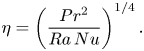 \begin{equation} \eta = \left(\frac{Pr^2}{Ra \, Nu}\right)^{1/4}. \end{equation}
To obtain (A 1), we first take the dot product of the dimensional momentum equation with  $\boldsymbol {u}$, giving
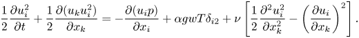 \begin{equation} \frac{1}{2} \frac{\partial u_i^2}{\partial t} + \frac{1}{2} \frac{\partial (u_k u_i^2)}{\partial x_k} = - \frac{\partial (u_i p)}{\partial x_i} + \alpha g w T \delta_{i2} + \nu \left[\frac{1}{2}\frac{\partial^2 u_i^2}{\partial x_k^2} - \left(\frac{\partial u_i}{\partial x_k}\right)^2\right]. \end{equation}
Taking the long time and area average of (A 2), we obtain
 \begin{equation} \epsilon \equiv \nu \langle|\boldsymbol{\nabla} \boldsymbol{u}|^2\rangle = \alpha g \left\langle w T\right\rangle. \end{equation}
Using  $\left \langle w T\right \rangle = \epsilon /(\alpha g) \approx \kappa {\rm \Delta} T/H \times Nu$ in the expression for the dimensional Kolmogorov length scale ( $\eta = (\nu ^3/\epsilon )^{1/4}$) and after some algebra and rearrangement, we obtain (A 1).
A criterion for a simulation to be well resolved is (Grötzbach Reference Grötzbach1983)
 \begin{equation} N_G = \frac{{\rm \pi} \eta}{h} > 1, \end{equation}
where  $h = \sqrt {{\rm \Delta} x {\rm \Delta} z}$, where ${\rm \Delta} x$ and ${\rm \Delta} z$ are mesh sizes along the horizontal and vertical directions. (All length scales are non-dimensionalized using the height of the cell.) We use uniform grids in our simulations, so ${\rm \Delta} x = {\rm \Delta} z$ and $h = {\rm \Delta} z$. In table 1, we show the computed values of $\eta$ for the six highest $Ra$ for $p = -1.5$. It is clear from table 1 that the resolutions used by us are able to resolve the Kolmogorov length scale – both in the interior and in the boundary layers. Note that we have used a more stringent criterion than (A 4) as we show that $N_{\eta } > 1$ as well as $N_G > 1$.
Table 1. Comparison of mesh size with the Kolmogorov length scale for the highest six  $Ra$ and $p = -1.5$. The Kolmogorov length scale is calculated using (A 1).

A.2. Spatial resolution: boundary layers
We estimate the non-dimensional boundary-layer thickness,  $\delta _T$, using
 \begin{equation} \delta_T = \frac{1}{2 Nu}.\end{equation}
Table 2 shows the boundary-layer thickness for all  $Ra$ for $p = -1.5$ and the number of grid points within the boundary layer. It is clear from the table that in our simulations there are at least $8$ grid points within the boundary layer. To further demonstrate this point, we show the time and horizontally averaged temperature profiles for $Ra = 2.15 \times 10^9$ and $Ra = 10^{10}$ and $p = -1.5$ in figure 8. There are $9$ grid points in each of the two boundary layers, in agreement with the estimate in table 2.
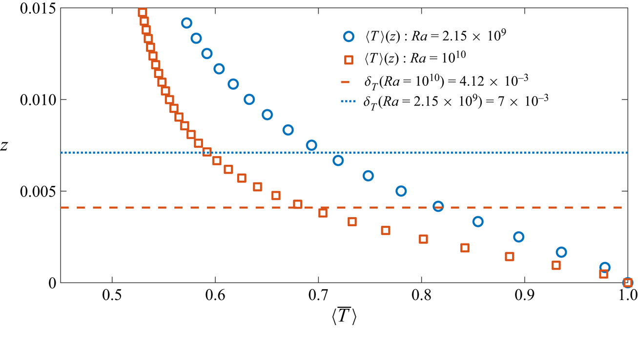
Figure 8. Horizontally and temporally averaged temperature profiles for  $Ra = 2.15 \times 10^9$ (circles) and $Ra = 10^{10}$ (squares) and $p = -1.5$. The dotted and dashed lines show the boundary-layer thicknesses for $Ra = 2.15 \times 10^9$ and $Ra = 10^{10}$, respectively. There are $9$ grid points in each boundary layer. The kinks at $z=0$ are associated with the use of the mid-grid bounceback condition to impose no-slip and no-penetration boundary conditions in the lattice Boltzmann method. This version of the bounceback renders the effective wall to be between the first and second grid points (Succi Reference Succi2001). Hence, the no-slip boundary condition effectively applies at a distance $z = {\rm \Delta} z/2$, where ${\rm \Delta} z$ is the grid size, above $z=0$ where the temperature boundary condition is imposed. The calculation of $Nu$ at the boundary takes this into account, and has been tested by reproducing the $Nu(Ra)$ results from spectral simulations for flat boundaries (Toppaladoddi et al. Reference Toppaladoddi, Succi and Wettlaufer2015a).
Table 2. Comparison of boundary-layer thickness and the resolutions used.
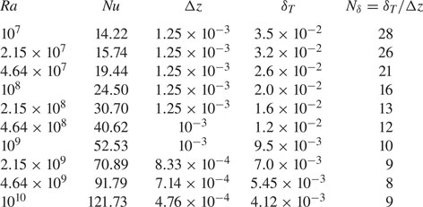
Table 3. The  $Nu(Ra)$ data for four different realizations of rough boundary for $p = -3.0$. The different realizations are numbered as $r=1,\ldots ,4$.
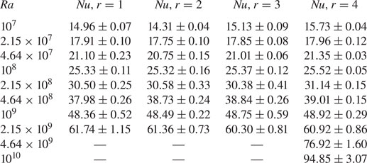
Table 4. The  $Nu(Ra)$ data for four different realizations of rough boundary for $p = -2.0$. The different realizations are numbered as $r=1,\ldots ,4$.
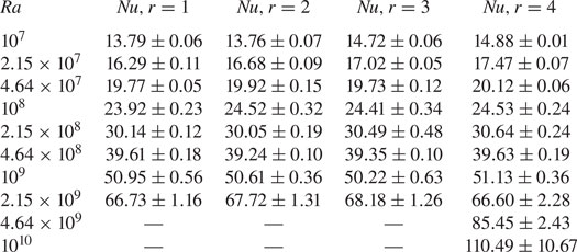
Table 5. The  $Nu(Ra)$ data for four different realizations of rough boundary for $p = -1.5$. The different realizations are numbered as $r=1,\ldots ,4$.
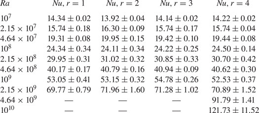
Table 6. The  $Re(Ra)$ data for four different realizations of rough boundary for $p = -3.0$. The different realizations are numbered as $r=1,\ldots ,4$.
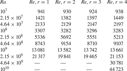
Table 7. The  $Re(Ra)$ data for four different realizations of rough boundary for $p = -2.0$. The different realizations are numbered as $r=1,\ldots ,4$.
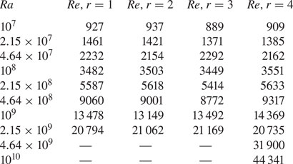
Table 8. The  $Re(Ra)$ data for four different realizations of rough boundary for $p = -1.5$. The different realizations are numbered as $r=1,\ldots ,4$.
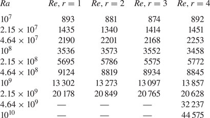
A.3. Temporal convergence
To ascertain that a time window of  $200$ time units was sufficient to obtain converged statistics, we ran simulations for $Ra = 2.15 \times 10^9$ and $p = -1.5$ with the same spatial resolution for two durations: (i) $t \approx 390$ and (ii) $t \approx 830$. In figure 9 we show a moving average of the $Nu(t)$ data measured at $z/H = 0.42$, where $H$ is the height of the cell for the two cases. The window for the moving average is $200$ time units.It is seen that the moving average value of $Nu$ is approximately constant beginning at $t \approx 220$. There are fluctuations in the curves and the maximum and minimum variations in the fluctuations are approximately 4 % of the mean. For the shorter duration run, which was averaged over $200$ time units, $\left \langle \overline {Nu}\right \rangle = 70.89$, and for the longer duration run, which was averaged over $613$ time units, $\left \langle \overline {Nu}\right \rangle = 69.81$. The difference between the two values is 1.5 %.
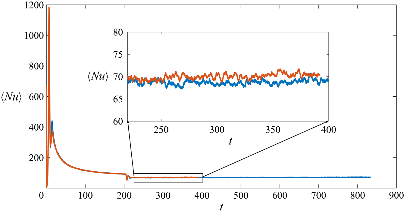
Figure 9. A 200 time-unit moving average of the  $Nu(t)$ data measured at $z/H = 0.42$ for two simulations of different duration with the same roughness profile, $p = -1.5$ and $Ra = 2.15 \times 10^9$.
Appendix B. Characteristic length scale
Here we consider the impact of an alternative definition of the characteristic length scale used in the non-dimensionalization. Let  $H_1$ be the characteristic length scale that gives $Nu_1=1$ at $Ra = 0$. The definition of $Nu$ used above is
 \begin{equation} Nu = \frac{Q H}{k {\rm \Delta} T}, \end{equation}
where  $Q$ is the total heat flux, $H$ is the depth of the cell, and ${\rm \Delta} T$ is the temperature difference between top and bottom boundaries. This can be written as
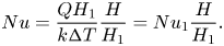 \begin{equation} Nu = \frac{Q H_1}{k {\rm \Delta} T} \frac{H}{H_1} = Nu_1 \frac{H}{H_1}. \end{equation}
By design,  $Nu_1 = 1$ at $Ra = 0$, and hence
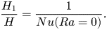 \begin{equation} \frac{H_1}{H} = \frac{1}{Nu(Ra=0)}. \end{equation}
Performing simulations for  $Ra = 0$ and all values of $p$ used, we find that $Nu = 1.06$ for $p = -1.5$ and $-2$ and $Nu = 1.05$ for $p=-3$. This implies that the effective length scale ( $H_1$) from (B 3) is ${\approx } 95\,\%$ of the depth of the cell. We can now use this new scale, $H_1$, to calculate the re-scaled values of the Rayleigh and Nusselt numbers, which are given by
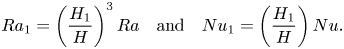 \begin{equation} Ra_1 = \left(\frac{H_1}{H}\right)^3 Ra \quad \text{and}\quad Nu_1 = \left(\frac{H_1}{H}\right) Nu. \end{equation}
Figure 10 shows  $Nu_1(Ra_1)$, $Nu(Ra)$, and the linear least-squares fits over the last seven data points for the respective data sets for $p=-1.5$. The fit for the new data over the highest seven $Ra$ gives $Nu_1 = 0.037 \times Ra_1^{0.352 \pm 0.011}$, which is the same for the corresponding fit $Nu=0.037 \times Ra^{0.352 \pm 0.011}$ using the length scale $H$. This is easily seen in figure 10. Similar analyses have been performed for data sets for other values of $p$, and these conclusions remain the same for those data sets as well with $H_1/H=0.95$ for all values of $p$ considered here. Moreover, the pre-factor changes by less than 1 % because $H_1/H = 0.95$, which is close to unity.
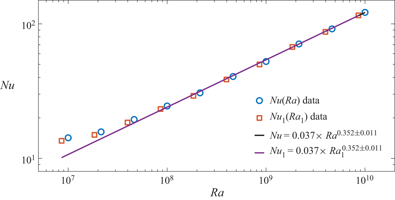
Figure 10. The  $Nu_1(Ra_1)$ and $Nu(Ra)$ data sets along with their power-law fits for $p=-1.5$.
Hence, although the choice of  $H_1$ is relevant if one requires that the Nusselt number is $1$ in the conductive state, choosing $H$ as the length scale does not impact the scaling results reported for the turbulent heat transport for any value of $p$ used in this study in any appreciable way.
Appendix C. Effect of increased area on heat transport
To understand the contribution of increased surface area to the transport of heat, we compute the ratio  $A_f/A_0$ (effective area) and $Nu/Nu_0$ (effective heat transport). Here, $A_f$ is the effective transfer area given by the surface area of $min[h(x),1-\delta _T]$, which increases the effective area to account for regions where the fractal boundary at $z=h(x)$ protrudes beyond the boundary-layer thickness $\delta _T$; $A_0$ is the area of the flat boundary; and $Nu_0$ is the value of the Nusselt number for a flat boundary. The boundary-layer thickness is estimated using (A 5) and the values of $Nu_0$ are obtained using the power law: $Nu_0 = 0.138 \times Ra^{0.285}$ (Johnston & Doering Reference Johnston and Doering2009). The values of $A_f/A_0$ calculated in this way are monotonic functions of $Ra$, so that as the thermal boundary layer thins, more of the fractal boundary is exposed to the flow. This is shown in figure 11 for all values of $p$ (i.e. as $p$ increases from $-3$ to $-1.5$).Note that the curves appear to saturate at the higher end of $Ra$ because we have computed the Steinhaus series (Rothrock & Thorndike Reference Rothrock and Thorndike1980) only up to a large finite wavenumber. For each $Ra$, the effective area increases for increasing value of $p$, showing that the boundaries become more rough.
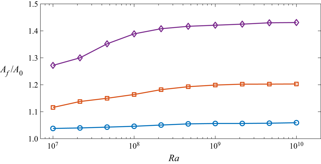
Figure 11. Ratio  $A_f/A_0$ of effective transfer area to that of flat boundary as a function of $Ra$ for different values of $p$:
$p$:  $p=-3$ (circles); $p=-2$ (squares); and $p=-1.5$ (diamonds).
In figures 12(a)–12(c), we show  $Nu/Nu_0$ as a function of $A_f/A_0$ for all $Ra$ and $p$. In each of these figures the first point, with the lowest $A_f/A_0$, corresponds to $Ra = 10^7$, the second to $Ra = 2.15 \times 10^7$,…, and the last one, with the largest $A_f/A_0$ value, to $Ra = 10^{10}$. (See figure 11.) The following observations can be made from figures 12(a)–12(c): (a) $Nu/Nu_0$ varies non-monotonically with $A_f/A_0$ showing the effect of the exposure of the fractal boundary to the outer flow; and (b) the difference in $A_f/A_0$ values for the last three data points for $p=-2$ and $p=-1.5$ is very small, but there is a relatively substantial increase in $Nu/Nu_0$ for these values.
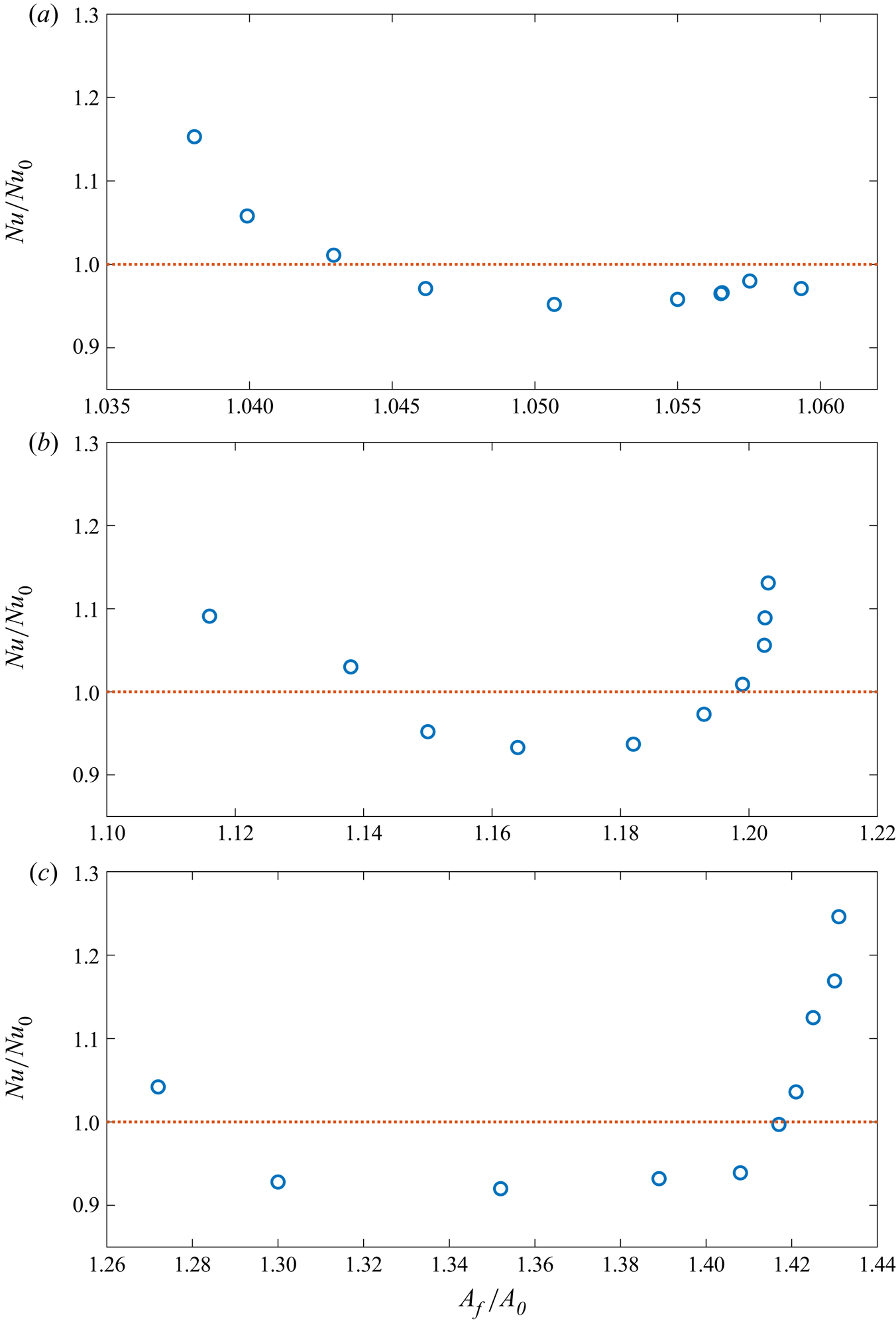
Figure 12. Plots of  $Nu/Nu_0$ versus $A_f/A_0$ for: (a) $p = -3$; (b) $p=-2$; and (c) $p=-1.5$.
To determine if the increase in the effective area can explain the augmentation in heat flux, we plot the  $Nu(Ra)$ data for $p=-3, -2$ and $-1.5$ and the corresponding $Nu_f(Ra) = Nu_0(Ra) \times A_f(Ra)/A_0$ data for the same range of $Ra$ in figures 13(a)–13(c). If the increase in $Nu(Ra)$ values were solely due to the enhanced area, such that
 \begin{equation} Nu = Nu_0 \frac{A_f}{A_0} = Nu_f, \end{equation}
then the  $Nu(Ra)$ and $Nu_f(Ra)$ curves would coincide. It is seen from figures 13(a)–13(c) that: (a) the curves do not coincide; (b) the fractal boundary for $p=-3$ is hydrodynamically smooth for heat transport as the $Nu(Ra)$ and $Nu_f(Ra)$ curves are parallel for $Ra \ge 10^8$; (c) the curve for $Nu_f(Ra)$ does not explain the curvature that is seen at lower $Ra$ in the $Nu(Ra)$ data for any $p$; and (d) while the values of $\beta$ for the two simulated $Nu(Ra)$ curves are substantially different for $p=-2$ and $p=-1.5$, the corresponding fitted $\beta$ for $Nu_f(Ra)$ are independent of $p$, to within the uncertainty. Hence, we conclude that the increase in $\beta$ for convection over the fractal boundaries is because of a change in the dynamics, which is consistent with increased plume production (Stringano et al. Reference Stringano, Pascazio and Verzicco2006; Toppaladoddi et al. Reference Toppaladoddi, Succi and Wettlaufer2015a, Reference Toppaladoddi, Succi and Wettlaufer2017). This dynamics has been explicitly shown to be operative in previous direct numerical simulations of turbulent convection over periodic roughness of different wavelengths (Toppaladoddi et al. Reference Toppaladoddi, Succi and Wettlaufer2015a, Reference Toppaladoddi, Succi and Wettlaufer2017).
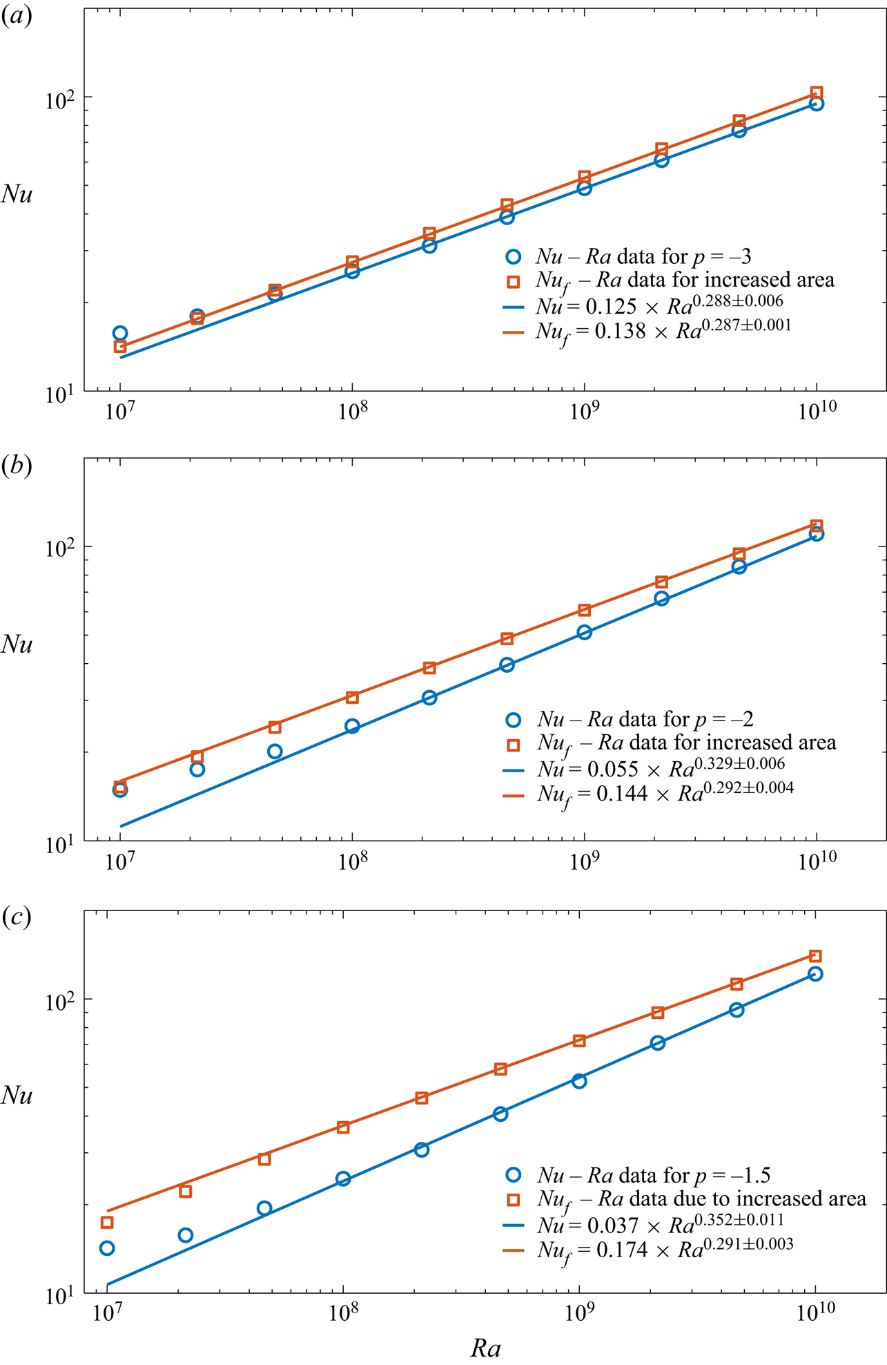
Figure 13. Heat flux data for the fractal boundaries ( $Nu$) and theory that applies heat flux for flat boundaries over an augmented area ( $Nu_f$): (a) $p = -3$; (b) $p=-2$; and (c) $p=-1.5$. The power-law fits are for the range $Ra \in [10^8, 10^{10}]$.


 Open access