


1. Introduction
Interfacial flows with insoluble or soluble surfactants are intensely studied in the recent literature (Manikantan & Squires Reference Manikantan and Squires2020), and the presence of the surface-active agent proves to have a decisive role on the stability characteristics and transitions, as well as on accompanying transport phenomena (Frenkel & Halpern Reference Frenkel and Halpern2002; Blyth & Pozrikidis Reference Blyth and Pozrikidis2004; Pereira et al. Reference Pereira, Trevelyan, Thiele and Kalliadasis2007; Craster & Matar Reference Craster and Matar2009; Kalogirou & Papageorgiou Reference Kalogirou and Papageorgiou2015; Katsiavria & Bontozoglou Reference Katsiavria and Bontozoglou2020; Hu, Fu & Yang Reference Hu, Fu and Yang2020; Constante-Amores et al. Reference Constante-Amores, Batchvarov, Kahouadji, Shin, Chergui, Juric and Matar2021; D'Alessio & Pascal Reference D'Alessio and Pascal2021; Samanta Reference Samanta2021). Of fundamental interest in such flows is the intricate coupling of the dynamics of the surfactant – i.e. surface elasticity and viscosity, adsorption–desorption kinetics – with the dynamics of the flow field. Quite frequently in micro-flows, the Reynolds number is very small and flow dynamics is dictated by the dynamics of the boundaries. Among the wide variety of applications, prominent is the study of various aspects of lung physiology, where thin, surfactant-laden films coat the airways and the alveoli (Gaver & Grotberg Reference Gaver and Grotberg1990; Halpern, Jensen & Grotberg Reference Halpern, Jensen and Grotberg1998; Matar, Zhang & Craster Reference Matar, Zhang and Craster2003; Grotberg Reference Grotberg2011; Kim et al. Reference Kim, Choi, Zasadzinski and Squires2011; Filoche, Tai & Grotberg Reference Filoche, Tai and Grotberg2015; Muradoglu et al. Reference Muradoglu, Romanò, Fujioka and Grotberg2019). In the case of alveoli, which is the focus of the present work, it is the periodic inflation and deflation of alveolar walls during the breathing cycle that drives the flow.
Lung alveoli are lined with a thin liquid layer, estimated as  $0.1\unicode{x2013}1\,\mathrm {\mu }{\rm m}$ thick, depending on lung inflation and health condition (Bastacky et al. Reference Bastacky, Lee, Goerke, Koushafar, Yager, Kenaga, Speed, Chen and Clements1995; Wei et al. Reference Wei, Fujioka, Hirschl and Grotberg2005). The interface of this layer, which is always in contact with the alveolar gas, is coated by a monolayer of special surface-active agents that constitute the pulmonary surfactant. The pulmonary surfactant is a combination of lipids and proteins, which – apart from populating the adsorbed monolayer – are also suspended in the liquid in the form of aggregates (Zuo et al. Reference Zuo, Veldhuizen, Neumann, Petersen and Possmayer2008). The surfactant acts to reduce drastically surface tension, making the alveoli more compliant and minimizing the metabolic work of breathing (Zasadzinski et al. Reference Zasadzinski, Ding, Warriner, Bringezu and Waring2001; Rugonyi, Biswas & Hall Reference Rugonyi, Biswas and Hall2008; Zhang et al. Reference Zhang, Wang, Fan and Zuo2011). In particular, the adsorbed surfactant monolayer is able to sustain large compressions during contraction, resulting in extremely low values of surface tension. This behaviour is accompanied by a rapid replenishment of the monolayer content during expansion, which restricts the increase of surface tension at the inhalation stage of the breathing cycle (Wüstneck et al. Reference Wüstneck, Wüstneck, Fainerman, Miller and Pison2001; Parra & Perez-Gil Reference Parra and Perez-Gil2015).
The hydrodynamics of the thin liquid layer lining the alveoli has been repeatedly the topic of investigation during the last decades (Gradon & Podgorski Reference Gradon and Podgorski1989; Podgorski & Gradon Reference Podgorski and Gradon1993; Espinosa & Kamm Reference Espinosa and Kamm1997; Zelig & Haber Reference Zelig and Haber2002; Wei et al. Reference Wei, Benintendi, Halpern and Grotberg2003, Reference Wei, Fujioka, Hirschl and Grotberg2005; Halpern et al. Reference Halpern, Fujioka, Takayama and Grotberg2008; Kang et al. Reference Kang, Chugunova, Nadim, Waring and Walther2018). The reason for this interest is that slow convective motions, which may develop triggered by the radial oscillation of the alveolar wall, are potentially of importance for lung homeostasis. In particular, it has been proposed that flow in the liquid lining may help cleanse the alveolus from deposited particles, and it may provide a potential route for cell–cell signalling. Such convective motions are also important when it is desired to transport macromolecules towards the alveoli, as for example in the clinical practices of surfactant replacement therapy and partial liquid ventilation.
From a different perspective, the interfacial motion of the liquid layer sets the true boundary condition for the airflow that enters and leaves the alveolus during breathing. In this respect, it is recalled that studies neglecting the liquid layer showed that chaotic mixing may occur inside the first alveolar generations, leading to enhanced particle transport and deposition (Tsuda, Henry & Butler Reference Tsuda, Henry and Butler1995, Reference Tsuda, Henry and Butler2008; Sznitman et al. Reference Sznitman, Heimsch, Wildhaber, Tsuda and Rosgen2009; Tsuda, Laine-Pearson & Hydon Reference Tsuda, Laine-Pearson and Hydon2011; Ciloglu Reference Ciloglu2020). It is of evident interest to consider how is the prediction of the airflow field modified by the inclusion of the liquid flow.
Analysis of the dynamics of an oscillating alveolus necessitates also consideration of its neighbourhood. It is recalled that, in generic lung models, alveoli start to appear beyond the 15th airway generation (respiratory bronchioles). They are scattered at first on the bronchiolar epithelium and gradually increase in density, until – beyond the 17th generation – airway ducts are fully covered by alveoli in close contact with each other (Weibel Reference Weibel1984; Tsuda et al. Reference Tsuda, Henry and Butler2008). The scattered alveoli are termed ‘type B’ and the densely packed ‘type A.’
It has been argued in the literature (Wei et al. Reference Wei, Benintendi, Halpern and Grotberg2003, Reference Wei, Fujioka, Hirschl and Grotberg2005) that different boundary conditions should apply for alveoli of type A and type B. For example, Gradon & Podgorski (Reference Gradon and Podgorski1989) model type B alveoli and pose constant values of film thickness and surfactant concentration at the rim. To model a type A alveolus, Wei et al. (Reference Wei, Benintendi, Halpern and Grotberg2003) also fix the film thickness at the rim but set the local flux equal to zero. Wei et al. (Reference Wei, Fujioka, Hirschl and Grotberg2005) focus on the strong surface tension limit, as in an alveolus with severe surfactant deficiency. They assume a film that is thick in the interior (flooded alveolus) but diminishes in thickness at the rim.
In all cases considered, the liquid layer lining the alveolus is modelled by quasi-steady Stokes flow, an approach which is justified by the very small velocities involved and the relatively slow time scale of breathing (Wei et al. Reference Wei, Fujioka, Hirschl and Grotberg2005; Kang et al. Reference Kang, Chugunova, Nadim, Waring and Walther2018). Two key mechanisms that may create shearing motion, i.e. velocities parallel to the alveolar epithelium, are Marangoni (elastic) stresses that result from spatial variation of surface tension and capillary stresses that result from spatial variation of interfacial curvature. Although surface tension is drastically lowered during a large part of the breathing cycle, the relative significance of Marangoni and capillary stresses is subject to discussion (Wei et al. Reference Wei, Benintendi, Halpern and Grotberg2003, Reference Wei, Fujioka, Hirschl and Grotberg2005; Kang et al. Reference Kang, Chugunova, Nadim, Waring and Walther2018).
Studies in the literature that aim at estimating the pattern and magnitude of shearing flow may be broadly classified in two categories, in relation to the posited deformation of the alveolar wall. In the first category, the epithelium is taken for simplicity as flat, with one end pinned and the other experiencing periodic motion in the tangential direction (Gradon & Podgorski Reference Gradon and Podgorski1989; Espinosa & Kamm Reference Espinosa and Kamm1997; Wei et al. Reference Wei, Benintendi, Halpern and Grotberg2003). Thus, the wall is subjected to non-uniform stretching, which – by the no-slip boundary condition – introduces directly a varying tangential velocity along the liquid layer.
In the second category, the alveolus is modelled as a spherical cap subjected to radial oscillation. In this case, the wall deformation is uniform and thus imparts no tangential motion to the liquid. The only way to break the radial symmetry is through appropriate boundary conditions. Thus, the boundary conditions at the rim emerge as a delicate component of the overall alveolar modelling. Positing constant film thickness or/and surfactant concentration at the rim (as in some previous works) forces the development of gradients with the inner interface, because the variation of the wall area during cap oscillation leads to inverse variation of film thickness and surfactant concentration inside the alveolus. However, the physical relevance of such boundary conditions is not always clear.
In the present work, the problem is studied in the spherical geometry and solved in the Stokes limit, using a lubrication approximation and extending the approach of Kang et al. (Reference Kang, Chugunova, Nadim, Waring and Walther2018). A new boundary condition is formulated for the alveolar rim, by matching the ‘large-scale’ dynamics of the alveolus to ‘small-scale’ equilibrium over the finite thickness of the mid-alveolar wall. The complex dynamics of the pulmonary surfactant is described by a recently developed model (Bouchoris & Bontozoglou Reference Bouchoris and Bontozoglou2021), which was found to predict with quantitative accuracy the surface tension–surface area hysteresis loops measured independently for various lung surfactant preparations (Saad, Neumann & Acosta Reference Saad, Neumann and Acosta2010; Xu, Yang & Zuo Reference Xu, Yang and Zuo2020).
Small-amplitude oscillations around the equilibrium conditions of the alveolus are considered. The simplification permits expansion of the equations and boundary conditions in the oscillation amplitude  $a$, and also allows a somewhat simpler treatment of the complex dynamics of the pulmonary surfactant. The resulting systems for the linear and the weakly nonlinear problem are solved by a standard Galerkin finite-element method and provide estimates of the pattern and size of shearing motions and of the modes of interaction between the rim and the interior of the alveolus. In particular, the significance of non-zero film thickness at the rim is demonstrated and the role of Marangoni and capillary stresses in determining the flow field is interrogated. The role of surfactant solubility is also investigated.
The paper is organized as follows. Governing equations and boundary conditions are derived in the lubrication approximation in § 2. In § 3, the equations are scaled and expanded with reference to the equilibrium conditions of a non-oscillating alveolus, and the numerical method is formulated. Results are presented and discussed in § 4 and concluding remarks are made in § 5.
2. Development of governing equations and boundary conditions
2.1. The flow problem
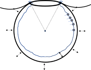
The alveolus is modelled as a spherical cap of periodically varying radius  $R(t)$ with an opening of angle $2 \theta _0$, as shown in figure 1(a). The truncated sphere is the most common model geometry, not only in the older but also in the recent literature (Kolanjiyil & Kleinstreuer Reference Kolanjiyil and Kleinstreuer2019). In particular, it has been argued (Harding & Robinson Reference Harding and Robinson2010), based on SEM images, that the apparent polygonal shape of alveoli is associated with non-uniform thickness of the wall septa, so that the actual airspace is closer to spherical. Also, there is evidence that the precise shape of the alveolus does not affect greatly the resulting flow and transport (Henry & Tsuda Reference Henry and Tsuda2010).

Figure 1. (a) Sketch of the spherical cap with the main problem parameters and (b) magnification of the rim (to be discussed in § 2.4). Note that  $h_0(t)=h(\theta _0,t)$ and $\varGamma _0(t)=\varGamma (\theta _0,t)$.
The liquid layer is considered Newtonian (Grotberg Reference Grotberg2011), with constant density  $\rho$ and viscosity $\mu$. Its flow field is assumed to be symmetric in the circumferential direction and is analysed in a spherical coordinate system $(r,\theta,\phi )$ located at the centre of the cap. Thus, the velocity in the liquid film is described as $\boldsymbol {u}(\boldsymbol {x},t)=(u_{r}(r,\theta,t),u_{\theta }(r,\theta,t),0)$ and the air–liquid interface is located at $r=r_s=R(t)-h(\theta,t)$, where $h(\theta,t)$ is the liquid film thickness and subscript ‘ $s$’ indicates value at the interface.
Following standard practice in the literature (Podgorski & Gradon Reference Podgorski and Gradon1993; Haber et al. Reference Haber, Butler, Brenner, Emmanuel and Tsuda2000; Zelig & Haber Reference Zelig and Haber2002; Wei et al. Reference Wei, Fujioka, Hirschl and Grotberg2005; Kang et al. Reference Kang, Chugunova, Nadim, Waring and Walther2018), the flow is posited to obey the continuity and the quasi-steady Stokes equation:
 \begin{gather} \boldsymbol{\nabla}\boldsymbol{\cdot} \boldsymbol{u}=0, \end{gather}
 \begin{gather} \mu\nabla^{2}\boldsymbol{u}=\boldsymbol{\nabla} p, \end{gather}
where  $p$ is the pressure field and gravitational effects are ruled out from the onset.
During breathing, the alveolus is taken to deform in a self-similar fashion, and thus the opening angle  $\theta _0$ remains constant. Following this assumption, Haber et al. (Reference Haber, Butler, Brenner, Emmanuel and Tsuda2000) and Wei et al. (Reference Wei, Fujioka, Hirschl and Grotberg2005) described the motion of the wall as
 \begin{equation} \boldsymbol{u}_w = \dot{R}( (1+\cos\theta \cos\theta_0) \,\boldsymbol{i}_r - \sin\theta \cos\theta_0 \,\boldsymbol{i}_{\theta} ) = \dot{R} \,\boldsymbol{i}_r + \dot{R}\cos\theta_0 \,\boldsymbol{i}_z = \boldsymbol{u}_{w,sym} + \boldsymbol{u}_{w,sb}, \end{equation}
where  $\boldsymbol {u}_{w,sym}$ represents a spherically symmetric oscillation and $\boldsymbol {u}_{w,sb}$ a time-dependent solid-body motion along the symmetry axis of the opening. It is presently desirable to describe the flow in a moving reference frame attached to the centre of the spherical cap. Such a reference frame is non-inertial, as $\boldsymbol {u}_{w,sb}$ varies with time, and would in general necessitate the introduction of a fictitious acceleration term, ${\rm d}\boldsymbol {u}_{w,sb}/{\rm d}t$, in the Navier–Stokes equation. However, in the quasi-steady Stokes limit, this term is negligible and may be omitted. Therefore, from now on, the wall motion is described only by the symmetric term $\boldsymbol {u}_{w,sym}= \dot {R} \,\boldsymbol {i}_r$.
Equations (2.1) and (2.2) are supplemented by the kinematic and the dynamic boundary conditions at the air/liquid interface, and by the no-slip condition on the alveolar wall. Liquid particles at the interface satisfy  $S(r,\theta,t)=r-R(t)+h(\theta,t)=0$ and the kinematic condition, ${\rm D}S/{\rm D}t=0$, becomes
 \begin{equation} \frac{\partial h}{\partial t}=\dot{R}(t)-u_r-\frac{u_{\theta}}{r}\frac{\partial h}{\partial \theta}. \end{equation}
The dynamic condition expresses the balance of forces at the interface and is given by
 \begin{equation} \boldsymbol{n} \boldsymbol{\cdot} \boldsymbol{\tau} ={-}p_{air}\boldsymbol{n} + \sigma (\boldsymbol{\nabla}_{s} \boldsymbol{\cdot} \boldsymbol{n})\,\boldsymbol{n} - \boldsymbol{\nabla}_s \sigma, \end{equation}
where  $\sigma$ is the local value of surface tension, $\boldsymbol {n}$ is the unit normal pointing towards the liquid, $\boldsymbol {\tau }=-p\boldsymbol {I}+\mu (\boldsymbol {\nabla } \boldsymbol {u}+\boldsymbol {\nabla } \boldsymbol {u}^{\mathrm {T}})$ is the stress tensor and $\boldsymbol {\nabla }_s=(\boldsymbol {I}-\boldsymbol {n}\boldsymbol {n})\boldsymbol {\cdot }\boldsymbol {\nabla }$ is the gradient along the interface. It is noted that (2.5) does not include rheological stresses, following experimental evidence (Wüstneck et al. Reference Wüstneck, Perez-Gil, Wüstneck, Cruz, Fainerman and Pison2005) that, for time scales relevant to breathing, phenomena can be characterized by only the elasticity modulus (i.e. the effect of surface viscosity is negligible). Finally, on the alveolar wall, $r=R(t)$, we have
 \begin{equation} u_{\theta} = 0, \quad u_r = \dot{R}(t) \end{equation}
and at  $\theta ={\rm \pi}$,
 \begin{equation} \left. \frac{\partial h}{\partial\theta}\right|_{\theta={\rm \pi}} = 0 \end{equation}
because of symmetry.
2.2. Conservation and dynamics of surfactant
Pulmonary surfactant is a mixture of lipids and proteins, which are practically insoluble in water. This mixture is presently modelled by a single generic surfactant, which mimics the dynamic behaviour of the actual preparation (Wüstneck et al. Reference Wüstneck, Perez-Gil, Wüstneck, Cruz, Fainerman and Pison2005). A monolayer forms at the interface, with the excess amount residing in the bulk in the form of aggregates (Zuo et al. Reference Zuo, Veldhuizen, Neumann, Petersen and Possmayer2008; Bykov et al. Reference Bykov, Milyaeva, Isakov, Michailov, Loglio, Miller and Noskov2021). The surface concentration of surfactant is described by the function  $\varGamma (\theta,t)$, whose spatial variation along the interface couples the flow and mass transfer problems through the dynamic boundary condition, (2.5). Thus,
 \begin{equation} \boldsymbol{\nabla}_s \sigma = \frac{{\rm d}\sigma}{{\rm d}\varGamma}\,\boldsymbol{\nabla}_s \varGamma, \end{equation}
where surface tension is related to the local surface concentration,  $\sigma =\sigma (\varGamma )$, through the equation of state of the surfactant, to be developed shortly. The sensitivity of $\sigma$ to $\varGamma$ is expressed by the Gibbs elasticity, $E$, where
 \begin{equation} E ={-}\frac{{\rm d}\sigma}{{\rm d}\ln\varGamma} ={-}\varGamma \frac{{\rm d}\sigma}{{\rm d}\varGamma}. \end{equation}
Mass conservation is imposed by the following equation (Stone Reference Stone1990; Wong, Rumschitzki & Maldarelli Reference Wong, Rumschitzki and Maldarelli1996; Pereira & Kalliadasis Reference Pereira and Kalliadasis2008):
 \begin{equation} \frac{\partial \varGamma}{\partial t} + \boldsymbol{u}\boldsymbol{\cdot}\boldsymbol{\nabla}_{\theta\phi}\varGamma + \varGamma (\boldsymbol{\nabla}_{s}\boldsymbol{\cdot}\boldsymbol{u}) = \mathcal{D}_{s} \boldsymbol{\nabla}_{s}^{2}\varGamma + j_b. \end{equation}
Equation (2.10) takes into account convection and diffusion along the interface, and mass exchange,  $j_b$, between the interface and the bulk. The latter is assumed to be governed by a kinetic resistance at the interface (rather than by diffusion), an assumption which is strongly supported by the literature (Ingenito et al. Reference Ingenito, Mark, Morris, Espinosa, Kamm and Johnson1999; Saad et al. Reference Saad, Neumann and Acosta2010). As the typical surfactant loading is many orders of magnitude higher than the critical micelle concentration of the monomer, and the effect of bulk diffusion is taken to be negligible, there is no need for a mass balance in the bulk. Boundary conditions for $\varGamma$ are applied at $\theta ={\rm \pi}$ and $\theta =\theta _0$. The former is determined by symmetry,
 \begin{equation} \left. \frac{\partial\varGamma}{\partial\theta}\right|_{\theta={\rm \pi}} = 0 , \end{equation}
but discussion and justification of the latter is postponed until § 2.4.
Surfactant equilibrium is taken to obey a Langmuir isotherm,
 \begin{equation} KC_{10}=\frac{\varGamma_{eq}}{\varGamma_{\infty,eq}-\varGamma_{eq}}, \end{equation}
where  $\varGamma _{\infty,eq}$ is the surface concentration at interfacial saturation, $K$ is the equilibrium constant and $C_{10}$ the critical micelle concentration of the monomer in the bulk. Thus, mass exchange with the bulk is expressed as follows in terms of an adsorption rate, $k_{ads}$:
 \begin{equation} j_b = k_{ads}C_{10}\left[(\varGamma_{\infty}-\varGamma)-\frac{\varGamma}{K\,C_{10}} \right]. \end{equation}
 A novel feature of the surfactant model is the inclusion of an intrinsic compressibility,  $\alpha$, of the adsorbed monolayer, as defined and justified by Fainerman, Miller & Kovalchuk (Reference Fainerman, Miller and Kovalchuk2002); Kovalchuk et al. (Reference Kovalchuk, Loglio, Fainerman and Miller2004, Reference Kovalchuk, Miller, Fainerman and Loglio2005). More specifically, the molar surface area, $\varOmega$, is taken to vary linearly with surface pressure, $\varPi =\sigma _0-\sigma$, according to the relation
 \begin{equation} \varOmega = \varOmega_{0} (1-\alpha \varPi), \end{equation}
where  $\sigma _0$ is the surface tension of pure water and $\varOmega _0$ is the molar area at zero surface pressure. This correction is particularly significant for dense monolayers and was recently shown to offer quantitative agreement of model dynamics with laboratory measurements using actual pulmonary preparations (Bouchoris & Bontozoglou Reference Bouchoris and Bontozoglou2021).
In terms of  $\varOmega$, the monolayer coverage, $\gamma$, is $\gamma =\varGamma \varOmega$, and thus the surface concentration at interfacial saturation, $\varGamma _{\infty }$, varies with surface pressure, and is given by
 \begin{equation} \varGamma_{\infty} = \frac{1}{\varOmega} = \frac{1}{\varOmega_{0}(1-\alpha \varPi)}. \end{equation}
Combining Langmuir isotherm, (2.12), with Gibbs theory – which is valid for a Gibbs dividing surface and an ideal bulk phase – the following equation of state is derived (Kovalchuk et al. Reference Kovalchuk, Loglio, Fainerman and Miller2004):
 \begin{equation} \frac{\varPi\varOmega_0}{\mathcal{R}\mathcal{T}}\left(1-\alpha\frac{\varPi}{2}\right) ={-}\ln(1-\gamma), \end{equation}
where  $\mathcal {R}$ is the gas constant and $\mathcal {T}$ the absolute temperature. Substituting the equation of state, (2.16), in the definition of Gibbs elasticity, (2.9), the following result is obtained:
 \begin{equation} \frac{1}{E}=\frac{\varOmega_0}{\mathcal{R}\mathcal{T}}\frac{(1-\alpha\varPi)(1-\gamma)}{\gamma}+\frac{\alpha}{1-\alpha\varPi}. \end{equation}
Equation (2.17) represents two elasticity mechanisms in series, the first of which is compositional, i.e. related to variations in surface concentration, and the second is intrinsic, i.e. related to the surface compressibility of the monolayer. Upon saturation (i.e.  $\gamma \rightarrow 1$), the interface retains finite elasticity due to the intrinsic contribution. It is noted that the application of simple isotherms, such as Frumkin or Langmuir, without the compressibility correction, gives at close packings unrealistically high values of Gibbs elasticity, which tend to infinity at saturation (Warszynski, Wantke & Fruhner Reference Warszynski, Wantke and Fruhner1998).
2.3. Lubrication approximation
The equations and boundary conditions of the problem are simplified by invoking a lubrication approximation (Leal Reference Leal2007). The mathematical procedure for the spherical geometry was outlined long ago by Podgorski & Gradon (Reference Podgorski and Gradon1993) and was more recently exposed in detail by Kang et al. (Reference Kang, Chugunova, Nadim, Waring and Walther2018). Thus, we present a brief outline and emphasize only the key points and the final results.
Integrating the equation of continuity in the  $r$-direction, and combining with the kinematic boundary condition and the wall velocity in the $r$-direction, the following evolution equation is derived:
 \begin{equation} (R-h)^2 \,\frac{\partial h}{\partial t} + (2Rh-h^2)\dot{R} + \frac{1}{\sin\theta}\frac{\partial}{\partial \theta}\int_{R-h}^{R} ru_{\theta}\sin\theta\,{\rm d}r = 0. \end{equation}
The lubrication form of the Navier–Stokes equations in spherical coordinates is
 \begin{gather} \frac{\partial p}{\partial r} = 0, \end{gather}
 \begin{gather} \mu\frac{\partial}{\partial r} \left(r^2\,\frac{\partial u_{\theta}}{\partial r}\right) = r\frac{\partial p}{\partial \theta}, \end{gather}
where gravitational effects are neglected (Espinosa & Kamm Reference Espinosa and Kamm1997). Combining (2.19) with the normal force boundary condition at the interface, and taking into account that viscous stresses are negligible in the lubrication approximation (Wei et al. Reference Wei, Fujioka, Hirschl and Grotberg2005; Kang et al. Reference Kang, Chugunova, Nadim, Waring and Walther2018), pressure across the film is derived as
 \begin{equation} p(\theta,t) =p_{air}-\sigma\boldsymbol{\nabla}_{s} \boldsymbol{\cdot} \boldsymbol{n}= p_{air} - \sigma\left[\frac{2}{R}+\frac{2\,h}{R^2}+\frac{1}{R^2\sin\theta}\frac{\partial}{\partial \theta}\left(\sin\theta\,\frac{\partial h}{\partial\theta}\right)\right]. \end{equation}
 Thus, (2.20) is readily integrated in the  $r$-direction and gives
 \begin{equation} u_{\theta}=\frac{r}{2\mu}\frac{\partial p}{\partial \theta}-\frac{C_{1}}{r}+C_{2}. \end{equation}
Integration constants  $C_{1}, C_{2}$ are determined by the tangential no-slip condition on the wall and the tangential force balance on the interface, the latter expressed in the lubrication approximation as
 \begin{equation} \mu\, r\frac{\partial}{\partial r}\left(\frac{u_{\theta}}{r}\right)={-}\frac{1}{r}\frac{\partial \sigma}{\partial \theta} \quad \mathrm{at} \ r=R(t)-h(\theta,t). \end{equation}
Thus, again in the lubrication limit,
 \begin{gather} C_1={-}\frac{1}{2\mu}\frac{\partial p}{\partial \theta}\,R^2\left(1-\frac{2h}{R}\right) - \frac{1}{\mu}\frac{\partial \sigma}{\partial \theta}R\left(1-\frac{2h}{R}\right), \end{gather}
 \begin{gather} C_2={-}\frac{1}{\mu}\frac{\partial p}{\partial \theta}R\left(1-\frac{h}{R}\right) - \frac{1}{\mu}\frac{\partial \sigma}{\partial \theta}\left(1-\frac{2h}{R}\right). \end{gather}
 Substituting the above results for  $u_{\theta }$ in (2.18), performing the integration and taking the lubrication limit results in the following evolution equation for the liquid film thickness, which is identical with that derived by Kang et al. (Reference Kang, Chugunova, Nadim, Waring and Walther2018):
 \begin{align} &\frac{\partial h}{\partial t} + \frac{2h\dot{R}}{R} - \frac{1}{R^2\sin\theta}\frac{\partial}{\partial\theta}\left(\frac{h^3\sin\theta}{3\mu}\frac{\partial p}{\partial\theta}-\frac{h^2\sin\theta}{2\mu}\frac{\partial\sigma}{\partial\theta}\right)\nonumber\\ &\quad = \frac{\partial h}{\partial t} + \frac{2h\dot{R}}{R} + \frac{1}{R^2\sin\theta}\frac{\partial}{\partial\theta}\left(\frac{Q}{2{\rm \pi}}\right) = 0, \end{align}
where  $Q(\theta,t)$ is the volumetric flow rate along the entire $\phi$-circumference at an elevation $z=R\cos \theta$, evaluated in the lubrication limit.
 \begin{equation} Q(\theta,t)=2{\rm \pi} R\sin\theta\int_{R-h}^{R} u_{\theta}\,{\rm d}r. \end{equation}
 A similar evolution equation is derived for the surface concentration,  $\varGamma$, of the surfactant by simplifying (2.10) according to the lubrication approximation. The respective result is
 $$\begin{gather} \frac{\partial\varGamma}{\partial t} + \frac{2\varGamma\dot{R}}{R} - \frac{1}{R^2\sin\theta}\frac{\partial}{\partial\theta}\left(\frac{\varGamma h^2\sin\theta}{2\mu}\frac{\partial p}{\partial\theta}-\frac{\varGamma h\sin\theta}{\mu}\frac{\partial\sigma}{\partial\theta}\right) - \frac{\mathcal{D}_s}{R^2\sin\theta}\frac{\partial}{\partial\theta}\left(\sin\theta\,\frac{\partial\varGamma}{\partial\theta}\right) \nonumber\\ =\frac{\partial\varGamma}{\partial t} + \frac{2\varGamma\dot{R}}{R} + \frac{1}{R^2\sin\theta}\frac{\partial}{\partial\theta}\left(\frac{Q_{\varGamma}}{2{\rm \pi}}\right) = j_b, \end{gather}$$
where  $Q_{\varGamma }(\theta,t)$ is the interfacial flow rate of surfactant along the entire $\phi$-circumference at an elevation $z=R\cos \theta$, evaluated in the lubrication limit.
 \begin{equation} Q_{\varGamma}(\theta,t)=2{\rm \pi} R\sin\theta\left(u_s\varGamma-\frac{\mathcal{D}_s}{R} \frac{\partial\varGamma}{\partial\theta}\right) \end{equation}
and  $u_s$ is the interfacial water velocity,
 \begin{equation} u_s={-}\frac{1}{2\mu}\frac{\partial p}{\partial\theta}\frac{h^2}{R}+\frac{1}{\mu}\frac{\partial\sigma}{\partial\theta}\frac{h}{R}. \end{equation}
 Equations (2.26) and (2.28) come to their final form by substitution of pressure from (2.21). This will be undertaken in the following section, after performing a change of independent variable. However, there is a subtle point related to this substitution, which was noted by Kang, Nadim & Chugunova (Reference Kang, Nadim and Chugunova2017) and is worth mentioning. When taking the derivative of (2.21) with respect to  $\theta$, additional terms containing $\partial \sigma /\partial \theta$ seem to come into play. However, these terms are of higher order in the ratio $(h/R)$ than the original $\partial \sigma /\partial \theta$ term in (2.26) and (2.28), and are thus negligible in the lubrication approximation.
2.4. Selection of boundary conditions at the alveolar rim
It has already been argued that the boundary conditions imposed at the rim of the spherical cap have a strong influence on the resulting dynamics. However, it appears that their physical origin is to some extent uncertain. For example, Gradon & Podgorski (Reference Gradon and Podgorski1989) set constant values of  $h$ and $\varGamma$ in their pioneering work modelling type B alveoli. They justify their choice by arguing that bronchioles are less extensible than alveoli, because – as they claim – the former change their surface area in proportion to their diameter and the latter in proportion to their square. However, it is presently accepted that bronchioles are equally extensible, because they expand/contract roughly isotropically, i.e. they also change in length (Darquenne & Paiva Reference Darquenne and Paiva1994; Choi & Kim Reference Choi and Kim2007). In later work, Podgorski & Gradon (Reference Podgorski and Gradon1993) neglect capillary forces and leave only the Marangoni term in their evolution equation for $h$. Thus, they apply a condition at the rim only for $\varGamma$, one based on a kind of ‘sketchy’ mass balance. Capillary forces are neglected also by Espinosa & Kamm (Reference Espinosa and Kamm1997), who set the flux of surfactant at the rim equal to zero.
Wei et al. (Reference Wei, Benintendi, Halpern and Grotberg2003) consider the effect of both Marangoni and capillary forces in their modelling of a type A alveolus. The conditions they impose are constant film thickness and zero liquid flux at the rim. Consequently, they employ a matching solution close to the rim, as the lubrication approximation locally breaks down because of the simultaneous existence of finite film thickness and zero flow rate. Wei et al. (Reference Wei, Fujioka, Hirschl and Grotberg2005) focus on the strong surface tension limit, as in an alveolus with severe surfactant deficiency, and thus take the interface to be spherical. They further assume a film that is thick in the interior (flooded alveolus) and diminishes in thickness at the rim. They admit however that at the rim, the film is actually ‘finite but thin’. In our understanding, the condition of constant film thickness at the rim appears physically questionable, given that the liquid thickness inside the alveolus changes continuously with time.
Before developing the presently proposed condition, two other interesting approaches are mentioned. Zelig & Haber (Reference Zelig and Haber2002) circumvent the direct definition of a boundary condition for  $h$. Instead, they use information about the average amount of surfactant expectorated and assume that the resulting mean per alveolus dictates the flow rate exiting at the alveolar rim. The more recent study of Kang et al. (Reference Kang, Chugunova, Nadim, Waring and Walther2018) includes, in the mass balance, source terms for surfactant production and degradation, however considers a complete sphere without an opening and a rim.
The present approach treats the rim of the alveolus as a region where liquid and surfactant may accumulate. Thus, the rate of inflow to (or outflow from) the alveolus is set equal to the accumulation rate over the rim. This approach is supported by two sets of microscopic observations. Characterizing microscopic sections by stereology, Vasilescu et al. (Reference Vasilescu, Gao, Saha, Yin, Wang, Haefeli-Bleuer, Ochs, Weibel and Hoffman2012) confirmed that the alveolar entrance rings are formed by strong fibre tracts in the free edges of the alveolar septa, resulting in rim thickness of a few micrometres.
Second, using low-temperature microscopy of anaesthetized rats, with their lungs inflated at 80 % of total lung capacity, Bastacky et al. (Reference Bastacky, Lee, Goerke, Koushafar, Yager, Kenaga, Speed, Chen and Clements1995) observed that the liquid lining of the alveolar epithelium is continuous over faces, ridges and protrusions. In particular, its area-weighted average thickness is approximately  $0.2\,\mathrm {\mu }{\rm m}$, and its thickness over protrusions and mid-alveolar walls is approximately half of that ( $0.09\,\mathrm {\mu }{\rm m}$).
Based on the above characteristics, the alveolar rim (assumed symmetric in the  $\phi$-direction) is taken to have a semi-circular cross-section of radius $r_0$, and to be covered by a liquid layer of finite and spatially uniform thickness, $h_0(t)$, which varies with time (figure 1b). Similarly, the rim is also characterized by a spatially uniform but time-varying surfactant concentration, $\varGamma _0(t)$. As $r_0\ll R$, the rim shrinks to a line when viewed in the ‘large-scale’ frame of the entire alveolus. Thus, $h_0(t)$ and $\varGamma _0(t)$ provide the boundary values for the system of evolution equations (2.26) and (2.28), i.e. $h_0(t)\equiv h(\theta _0,t)$ and $\varGamma _0\equiv \varGamma (\theta _0,t)$.
The final assumption, which permits closure of the problem, is that the dynamics of the layer covering the rim is entirely enslaved to the dynamics of the alveolar cap. Thus, only mass balances need to be satisfied, and the temporal variation of  $h_0$ and $\varGamma _0$ is dictated by the respective fluxes from/to the alveolus. The key assumptions in the above approach, i.e. the magnitude of the equilibrium film thickness at the rim, the spatial uniformity of film thickness and surfactant concentration over the rim, and the enslaved dynamics, will be further discussed and justified in § 5.
The mass balance of water at the rim is formulated, taking into account the symmetry in the  $\phi$-direction, and states that the volumetric flow rate towards the rim from adjacent alveoli equals the time change of water volume over the rim. Thus,
 \begin{equation} \left. \begin{gathered} -2Q(\theta_0,t) = \frac{{\rm d}}{{\rm d}t}\left[2{\rm \pi} R \sin\theta_0 \left({\rm \pi} \frac{(r_0+h_0)^2}{2}-{\rm \pi} \frac{r_0^2}{2}\right)\right] \\ \Rightarrow \quad -2\left.\int_{R-h}^{R} u_{\theta}\,{\rm d}r \right|_{\theta_0} = {\rm \pi}(r_0+h_0) \frac{{\rm d}h_0 }{{\rm d}t}+{\rm \pi} h_0 \left(r_0+\frac{h_0}{2}\right)\frac{\dot{R}}{R}, \end{gathered} \right\} \end{equation}
where subscript  $0$ signifies value at the rim, $x=x_0$. A similar mass balance for the surfactant, taking into account convection and diffusion along the interface and exchange by adsorption or desorption with the bulk, leads to the following expression:
 \begin{equation} \left. \begin{gathered} -2Q_{\varGamma}(\theta_0,t)+\left.2{\rm \pi} R\sin\theta_0{\rm \pi} (r_0+h_0) j_b\right|_{\theta_0}=\frac{{\rm d}}{{\rm d}t}\left[2{\rm \pi} R\sin\theta_0{\rm \pi}(r_0+h_0)\varGamma_0\right] \\ \Rightarrow\quad \left. -2\left(u_{s}\varGamma-\frac{\mathcal{D}_s}{R} \frac{\partial\varGamma}{\partial\theta}\right)\right|_{\theta_0} + \left.{\rm \pi}(r_0+h_0) j_b\right|_{\theta_0} = {\rm \pi}(r_0+h_0)\frac{{\rm d}\varGamma_0}{{\rm d}t}\\ \quad +{\rm \pi} \varGamma_0 \frac{{\rm d}h_0}{{\rm d}t}+{\rm \pi}\varGamma_0 (r_0+h_0)\frac{\dot{R}}{R}. \end{gathered} \right\} \end{equation}
The multiplier two in (2.31) and (2.32) accounts for alveoli of type A, i.e. flux coming to the rim from both sides of the mid-alveolar wall. Alveoli of type B are not presently considered, though it may be argued that a similar approach is applicable. The minus sign indicates flow in the negative  $\theta$-direction, i.e. towards the rim.
It is noted that loss terms could readily be incorporated in the boundary conditions, (2.31) and (2.32), to account for the possibility of water and surfactant entrainment from the rims by the airflow along the duct. Such a tentative entrainment mechanism resembles the suggestion of Zelig & Haber (Reference Zelig and Haber2002) and is in accord with recent findings that identify surfactant from the deep lung in the exhaled breath of human subjects (Oldham & Moss Reference Oldham and Moss2019). However, unlike the approach of Zelig & Haber (Reference Zelig and Haber2002), with the above boundary conditions, the flow of water and surfactant at the alveolar rim is not restricted by the entrainment rate.
3. Scaling, expansion around equilibrium and numerical solution
3.1. The final equations and the equilibrium solution
The problem is now described by (2.21), (2.26) and (2.28), subject to the aforementioned boundary conditions. However, following Kang et al. (Reference Kang, Nadim and Chugunova2017, Reference Kang, Chugunova, Nadim, Waring and Walther2018), it is more convenient to reformulate the system in terms of the new independent variable  $x=-\cos \theta$. Thus, pressure is expressed as
 \begin{equation} p(x,t) = p_{air}-\frac{2\sigma}{R}-\frac{\sigma}{R^2}\left[2h+\frac{\partial}{\partial x}\left((1-x^2)\frac{\partial h}{\partial x}\right)\right]. \end{equation}
 Transforming (2.26) and (2.28) in terms of  $x$, and substituting pressure from (3.1), the following final form of the evolution equations is obtained:
 $$\begin{gather} \frac{\partial h}{\partial t} + \frac{2h\dot{R}}{R} + \frac{1}{3\mu R^4}\frac{\partial}{\partial x}\left(\sigma h^3 (1-x^2) \frac{\partial}{\partial x}(2h+g)\right) \nonumber\\ + \frac{1}{2\mu R^2}\frac{\partial}{\partial x}\left(h^2 (1-x^2) \frac{{\rm d}\sigma}{{\rm d}\varGamma}\frac{\partial\varGamma}{\partial x}\right) = 0 \end{gather}$$
and
 $$\begin{gather} \frac{\partial\varGamma}{\partial t} + \frac{2\varGamma\dot{R}}{R}+ \frac{1}{2\mu R^4}\frac{\partial}{\partial x}\left(\varGamma h^2 (1-x^2)\,\sigma \frac{\partial}{\partial x}(2h+g)\right) \nonumber\\ +\frac{1}{\mu R^2}\frac{\partial}{\partial x}\left(\varGamma h (1-x^2) \frac{{\rm d}\sigma}{{\rm d}\varGamma}\frac{\partial\varGamma}{\partial x}\right) = \frac{\mathcal{D}_s}{R^2}\frac{\partial}{\partial x}\left((1-x^2)\frac{\partial\varGamma}{\partial x}\right)+j_b, \end{gather}$$
where  $D_{s}$ and $\mu$ are assumed constant, and we have defined
 \begin{equation} g(x,t)=\frac{\partial}{\partial x}\left((1-x^2)\frac{\partial h}{\partial x}\right). \end{equation}
The use of function  $g$ is not only intended to make the equations more compact, but is also necessary for the finite-element solution of the problem, as the definition of the new function $g(x,t)$ eliminates the higher than second-order derivatives in $h$.
$h$.
A reference frame for the present problem is the equilibrium film thickness,  $H(x)$, in a non-oscillating spherical cap of constant radius $\bar {R}$. Equilibrium requires that $\partial \sigma /\partial x=\partial p/\partial x=0$, i.e. the surfactant is equi-distributed and the interface is a perfect spherical cap, say of radius $R_s$. If the uniform capillary pressure is termed $\bar {p}$, (3.1) gives
 \begin{equation} 2H+\frac{\partial}{\partial x}\left((1-x^2)\frac{\partial H}{\partial x}\right) = \frac{p_{air}-\bar{p}}{\sigma}\bar{R}^2-2\bar{R}=2\bar{R}\left(\frac{\bar{R}}{R_s}-1\right)=2K. \end{equation}
Equation (3.5) has the trivial linear solution,  $H(x)=\kappa x +\lambda$, with $\kappa =(H_0-K)/x_0$ and $\lambda =K$ in terms of the constant $2K$ and the film thickness $H_0=H(x_0)$ at the rim of the cap $(x_0=-\cos \theta _0)$. Term $H_0$ is a key parameter for the problem, and its magnitude will be estimated from direct experimental evidence (Bastacky et al. Reference Bastacky, Lee, Goerke, Koushafar, Yager, Kenaga, Speed, Chen and Clements1995; Xu et al. Reference Xu, Yang and Zuo2020).
Parameter  $K$ is determined from the total volume of liquid in the cap, which in the lubrication limit is
 \begin{equation} V_{water} = 2{\rm \pi}\int_{\theta_0}^{\rm \pi}\int_{R-h}^R r^2\sin\theta\,{\rm d}r\,{\rm d}\theta \approx 2{\rm \pi} R^2\int_{\theta_0}^{\rm \pi} h(\theta)\sin\theta\,{\rm d}\theta = 2{\rm \pi} R^2\int_{x_0}^{1} h(x) \,{{\rm d}\kern0.06em x}. \end{equation}
Equivalently, a convenient input is the mean liquid film thickness,  $\bar {H}$, which is related to the liquid volume by the expression
 \begin{equation} V_{water} = 2{\rm \pi} R^2\left(1-x_0\right)\bar{H}. \end{equation}
 For a given total volume of water, a simple mass balance shows that the equilibrium film thickness,  $H(x)$, varies inversely with the square of the cap radius. Thus, it is verified by inspection that the function
 \begin{equation} h(x,t)=H(x)\,\frac{\bar{R}^2}{R^2(t)}, \end{equation}
together with a spatially uniform surface concentration of surfactant, satisfies (3.2) for arbitrary oscillation pattern,  $R(t)$. When $j_b\equiv 0$, the surface concentration has a similar form, $\varGamma (x,t)=\bar {\varGamma }[\bar {R}/R(t)]^2$, but when $j_b\neq 0$, it is a more complicated function of time (Manikantan & Squires Reference Manikantan and Squires2020). The above solution corresponds to a purely axial motion, i.e. with no gradients in the $\theta$-direction. However, the boundary conditions (2.31)–(2.32) are not satisfied, except for the special case $h(x_0,t)=0$. This behaviour is a first indication of the significance of the finite liquid film thickness at the rim in triggering tangential motion.
3.2. Scaling and dimensionless numbers
The characteristic scales used to non-dimensionalize the problem variables are mainly taken from the equilibrium conditions. Thus, we consider a motionless alveolar cap of radius  $\bar {R}$, coated by a liquid film whose mean thickness is $\bar {H}$. With these choices, the lubrication parameter is formally defined as
 \begin{equation} \epsilon=\frac{\bar{H}}{\bar{R}}. \end{equation}
The liquid is loaded by surfactant aggregates and equilibrates with an adsorbed monolayer of surface concentration  $\varGamma _{{eq}}$, which results in surface tension $\sigma _{eq}$ and surface elasticity $E_{eq}=- (\textrm {d}\sigma /\textrm {d}\ln \varGamma ) |_{\varGamma =\varGamma _{eq}}$. Finally, the characteristic time is the breathing period, $T$.
$T$.
With the above scales, the following dimensionless variables are defined:  $h^*=h/\bar {H}$, $H^*=H/\bar {H}$, $R^*=R/\bar {R}$, $t^*=t/T$, $\varGamma ^*=\varGamma /\varGamma _{eq}$, $\sigma ^*=\sigma /\sigma _{eq}$, $E^*=E/E_{eq}$, $p^*=p\,\bar {R}^2/(\sigma _{eq}\bar {H})$, $j_b^*=j_b T/\varGamma _{eq}$ and $g^*=g/\bar {H}$. Substituting the dimensionless variables, and also taking into account the definition of surface elasticity, (2.9), the system (3.2)–(3.3) is transformed as follows:
 \begin{equation} \frac{\partial h^*}{\partial t^*} + \frac{2h^*\dot{R^*}}{R^*} + \frac{1}{R^*} \frac{\partial F_h}{\partial x} = 0 \end{equation}
and
 \begin{equation} \frac{\partial\varGamma^*}{\partial t^*} + \frac{2\varGamma^*\dot{R^*}}{R^*}+ \frac{1}{R^*}\frac{\partial F_{\varGamma}}{\partial x}-j_b^* = 0, \end{equation}
where
 \begin{gather} F_h=\frac{Q^*}{R^*}=\epsilon^3\frac{Ca^{{-}1}}{3R^{*3}}\sigma^* h^{*3} (1-x^2) \frac{\partial}{\partial x}(2h^*+g^*)-\epsilon\frac{Ma}{2R^*}h^{*2}(1-x^2) \frac{E^*}{\varGamma^*}\frac{\partial\varGamma^*}{\partial x}, \end{gather}
 \begin{gather} F_{\varGamma}=\frac{Q_{\varGamma}^*}{R^*}=\epsilon^3\frac{Ca^{{-}1}}{2R^{*3}}\varGamma^*\sigma^* h^{*2} (1-x^2) \frac{\partial}{\partial x}(2h^*+g^*) \nonumber\\ -\epsilon\frac{Ma}{R^*}\varGamma^* h^*(1-x^2) \frac{E^*}{\varGamma^*}\frac{\partial\varGamma^*}{\partial x}- \frac{Pe_s^{{-}1}}{R^*}(1-x^2)\frac{\partial\varGamma^*}{\partial x} \end{gather}
and
 \begin{equation} j_b^* = St \left[ (\varGamma_{\infty}^*-\varGamma^*)-\frac{\varGamma^*}{KC_{10}}\right]. \end{equation}
Terms  $Q^*,\;Q_{\varGamma }^*$ are respectively the dimensionless volumetric water and interfacial surfactant flow rates, scaled by $\bar {Q}=2{\rm \pi} \bar {R}^2\bar {H}/T$ and $\bar {Q}_{\varGamma }=2{\rm \pi} \bar {R}^2 \varGamma _{eq}/T$.
The dimensionless numbers that appear in the above equations are
 \begin{equation} Ca^{{-}1}=\frac{\sigma_{eq}}{\mu(\bar{R}/T)} , \quad Ma=\frac{E_{eq}}{\mu(\bar{R}/T)}, \quad Pe_s^{{-}1}=\frac{\mathcal{D}_s T}{\bar{R}^2},\quad St=\frac{T}{1/(k_{{ads}}C_{10})}, \end{equation}
which are the inverse capillary number,  $Ca^{-1}$, that compares capillary to viscous stresses, the Marangoni number, $Ma$, that compares elastic to viscous stresses, the inverse Péclet number, $Pe_s^{-1}$, that compares surface diffusion to surface convection, and a Stanton number, $St$, that compares characteristic times of breathing and surfactant adsorption (Manikantan & Squires Reference Manikantan and Squires2020). The ratio of alveolar radius to breathing period that appears in these dimensionless numbers defines the characteristic velocity scale $\bar {U}=\bar {R}/T$.
With the above scaling and function definitions, the boundary conditions at the rim, (2.31) and (2.32), take the following dimensionless form:
 \begin{gather} -2F_h|_{x_{0}}=\sqrt{1-x_0^2}\;{\rm \pi}\left[\left(r_0^*+\epsilon h_0^*\right)\frac{{\rm d}h_0^*}{{\rm d}t^*}+h_0^*\left(r_0^*+\epsilon\frac{h_0^*}{2}\right)\frac{\dot{R}^*}{R^*}\right], \end{gather}
 \begin{gather} -2F_{\varGamma}|_{x_0}=\sqrt{1-x_0^2}\;{\rm \pi}\left[(r_0^*+\epsilon h_0^*)\left(\frac{{\rm d}\varGamma_0^*}{{\rm d}t^*}-j_{b0}^*\right)+\epsilon\varGamma_0^*\frac{{\rm d}h_0^*}{{\rm d}t^*}+\varGamma_0^*(r_0^*+\epsilon h_0^*)\frac{\dot{R}^*}{R^*}\right], \end{gather}
where subscript  $0$ signifies value at the rim, $x=x_0$, and $r_0^*=r_0/\bar {R}$ is the dimensionless radius of curvature of the rim. It is also noted that the symmetry boundary conditions at $\theta ={\rm \pi}$ are trivially satisfied in the present frame, provided the derivatives $\partial h/\partial x$ and $\partial \varGamma /\partial x$ are finite at $x=1$. Thus, (3.10) and (3.11), together with the above boundary conditions, (3.16), (3.17) and the model of surfactant dynamics (§ 2.2), provide the full description of the problem.
3.3. Expansion around equilibrium
The remainder of the paper focuses on the study of small-amplitude oscillations around equilibrium. This approach permits expansion of the above equations and boundary conditions, and is believed to provide solid results on the relative magnitude of tangential and radial motions, and on the modes of interaction between the interior and the rim of the alveolus. The full formulation of the problem that was developed in the previous sections will be used in the future, to investigate nonlinear phenomena under realistic breathing patterns.
The alveolar radius is considered to undergo small-amplitude oscillations
 \begin{equation} R^*(t^*)=1+a\,\mathrm{Re}[{\rm e}^{{\rm i}\,2{\rm \pi} t^*}] \end{equation}
with  $a\ll 1$. The dimensionless film thickness, $h^*$, its function $g^*$ and the surface concentration of surfactant, $\varGamma ^*$, are expanded as follows, to capture linear and weakly nonlinear effects,
 \begin{equation} \left. \begin{gathered} h^*(x,t^*)=H^*(x)+a\,\mathrm{Re}[h_1(x)\,{\rm e}^{{\rm i}\,2{\rm \pi} t^*}]+a^2\left(\mathrm{Re}[h_2(x)\,{\rm e}^{{\rm i}\,4{\rm \pi} t^*}]+h_S(x)\right),\\ g^*(x,t^*)=G^*(x)+a\,\mathrm{Re}[g_1(x) \,{\rm e}^{{\rm i}\,2{\rm \pi} t^*}]+a^2\left(\mathrm{Re}[g_2(x)\,{\rm e}^{{\rm i}\,4{\rm \pi} t^*}]+g_S(x)\right),\\ \varGamma^*(x,t^*)=1+a\,\mathrm{Re}[\varGamma_1(x)\,{\rm e}^{{\rm i}\,2{\rm \pi} t^*}]+a^2\left(\mathrm{Re}[\varGamma_2(x)\,{\rm e}^{{\rm i}\,4{\rm \pi} t^*}]+\varGamma_S(x)\right), \end{gathered} \right\} \end{equation}
with the above expressions calculated as  $\mathrm {Re}[z\textrm {e}^{\textrm {i}\,\phi }]=(z\textrm {e}^{\textrm {i}\,\phi }+\bar {z} \textrm {e}^{-\textrm {i}\,\phi })/2$. By indices $1,\,2,\,S$ is denoted the amplitude of each parameter in the respective order of approximation. Steady terms are included at second order to balance the ‘steady streaming’ resulting from products of first-order contributions. As a generic example, given two complex functions $z_1(x),\,w_1(x)$,
 \begin{equation} \mathrm{Re}[z_1 {\rm e}^{{\rm i}\,2{\rm \pi} t^*}] \cdot \mathrm{Re}[w_1 {\rm e}^{{\rm i}\,2{\rm \pi} t^*}]=\frac{1}{2}\mathrm{Re}[z_1w_1 {\rm e}^{{\rm i}\,4{\rm \pi} t^*}]+\frac{1}{2}\mathrm{Re}[z_1 \bar{w}_1]. \end{equation}
 Term  $G^*$, the equilibrium value of function $g^*(x,t^*)$, is eliminated by application of the equilibrium balance, (3.5), and the dimensionless fluxes, $F_h,\;F_{\varGamma }$, are expanded as
 \begin{gather} F_h=a\,\mathrm{Re}[F_{h1} {\rm e}^{{\rm i}\,2{\rm \pi} t^*}]+a^2\left(\mathrm{Re}[F_{h2} {\rm e}^{{\rm i}\,4{\rm \pi} t^*}]+F_{hS}\right), \end{gather}
 \begin{gather} F_{\varGamma}=a\,\mathrm{Re}[F_{\varGamma 1} {\rm e}^{{\rm i}\,2{\rm \pi} t^*}]+a^2\left(\mathrm{Re}[F_{\varGamma2} {\rm e}^{{\rm i}\,4{\rm \pi} t^*}]+F_{\varGamma S}\right), \end{gather}
where  $F_{hi},\ F_{\varGamma i},\ i=1,2,S$, are functions of $x$, given in terms of $h_i,\ g_i, \varGamma _i$ in Appendix A. The dimensionless mass exchange with the bulk, $j_b^*$, is also expanded as follows:
 $$\begin{gather} j_b^* = St_1\left( a\,\mathrm{Re}[\varGamma_1\,{\rm e}^{{\rm i}\,2{\rm \pi} t^*}]+a^2\mathrm{Re}[\varGamma_2 \,{\rm e}^{{\rm i}\,4{\rm \pi} t^*}]+a^2\varGamma_S\right) \nonumber\\ + a^2\,\frac{1}{4}St\, \varGamma_{\infty,\varGamma\varGamma}^*\left(\mathrm{Re}[\varGamma_1^2 \,{\rm e}^{{\rm i}\,4{\rm \pi} t^*}]+\varGamma_1\bar{\varGamma}_1\right), \end{gather}$$
where  $St_1$ is
 \begin{equation} St_1=St\left(\varGamma_{\infty,\varGamma}^*-1-\frac{1}{KC_{10}} \right) \end{equation}
with
 \begin{equation} \varGamma_{\infty,\varGamma}^*=\left.\frac{{\rm d}\varGamma_{\infty}^*}{{\rm d}\varGamma^*}\right|_{eq}, \quad \varGamma_{\infty,\varGamma\varGamma}^*=\left.\frac{{\rm d}^2\varGamma_{\infty}^*}{{\rm d}\varGamma^{*2}}\right|_{eq}. \end{equation}
It is noted that the surface concentration at close packing is not constant but is a function of surface pressure, and hence the derivatives in (3.23) and (3.24).
The following orders of the evolution equations result by straightforward substitution of the above into (3.10) and (3.11) and neglect of higher than second-order terms. Primes denote derivatives with respect to  $x$ and, as shown below, terms $F_{h1}',\,F_{\varGamma 1}'$ that appear in the second-order and steady equations are replaced by the respective first-order result.
 \begin{gather} 2{\rm \pi} {\rm i} h_1+F_{h1}'+4{\rm \pi} {\rm i}H^*=0, \end{gather}
 \begin{gather} 2{\rm \pi} {\rm i}\varGamma_1 +F_{\varGamma 1}'- St_1\varGamma_1+4{\rm \pi} {\rm i}=0, \end{gather}
 \begin{gather} 4{\rm \pi} {\rm i} h_2+2{\rm \pi} {\rm i} h_1-2{\rm \pi} iH^*+F_{h2}'-\frac{1}{2} F_{h1}'=0 \nonumber\\ \Rightarrow\quad 4{\rm \pi} {\rm i} h_2+3{\rm \pi} {\rm i} h_1+F_{h2}'=0, \end{gather}
 \begin{gather} 4{\rm \pi} {\rm i}\varGamma_2+2{\rm \pi} {\rm i}\varGamma_1-2{\rm \pi} {\rm i}+F_{\varGamma2}'-\frac{1}{2}F_{\varGamma1}'-St_1\varGamma_2-\frac{St}{4}\varGamma_{\infty,\varGamma\varGamma}^*\varGamma_1^2=0\nonumber\\ \Rightarrow\quad 4{\rm \pi} {\rm i}\varGamma_2+3{\rm \pi} {\rm i}\varGamma_1 + F_{\varGamma2}'-St_1\left(\varGamma_2+\frac{1}{2}\varGamma_1\right)-\frac{St}{4}\varGamma_{\infty,\varGamma\varGamma}^*\varGamma_1^2=0, \end{gather}
 \begin{gather} \mathrm{Re}\left[2{\rm \pi} {\rm i}\bar{h}_1\right]+F_{hS}'-\frac{1}{2}\mathrm{Re}\left[F_{h1}'\right]=0 \Rightarrow F_{hS}'+{\rm \pi}\,\mathrm{Im}\left[h_1\right]=0, \end{gather}
 \begin{gather} \mathrm{Re}\left(2{\rm \pi} {\rm i}\bar{\varGamma}_1\right)+ F_{\varGamma S}'-\frac{1}{2}\mathrm{Re}\left[F_{\varGamma1}'\right]- St_1\varGamma_S-\frac{St}{4}\varGamma_{\infty,\varGamma\varGamma}^* \mathrm{Re}\left[\varGamma_1 \bar{\varGamma}_1\right]=0\nonumber\\ \Rightarrow\quad F_{\varGamma S}'+{\rm \pi}\,\mathrm{Im}\left[\varGamma_1\right]- St_1\left(\varGamma_S+\frac{1}{2}\mathrm{Re}\left[\varGamma_1\right]\right)-\frac{St}{4}\varGamma_{\infty,\varGamma\varGamma}^* \left(\varGamma_1 \bar{\varGamma}_1\right)=0. \end{gather}
The system is completed by the expansions of  $g$
$g$
 \begin{equation} \left((1-x^2)h_i'\right)'-g_i=0 \quad i=1,2,S \end{equation}
and by the boundary conditions at  $x=x_0$. The latter are evaluated by expanding the right-hand side of (3.16), (3.17), and the respective coefficients $F_{hi}|_{x_0},\;F_{\varGamma i}|_{x_0},\ i=1,2,S$ are given in Appendix A.
3.4. Steady streaming of water and surfactant
The weakly nonlinear problem was formulated taking into consideration the possibility of steady streaming, with the inclusion of time-independent terms identified throughout the text by the subscript ‘ $S$.’ It will now be shown that steady streaming of water is always identically zero, as is also the steady streaming of insoluble surfactant. The exceptional (and important) case of a soluble surfactant is singled out, and will be considered further.
First, the dimensionless volumetric flow rate of water,  $Q^*=R^* F_h$, is calculated as follows:
 \begin{equation} Q^*=a\,\mathrm{Re}[F_{h1} \,{\rm e}^{{\rm i}\,2{\rm \pi} t^*}]+a^2\mathrm{Re}\left[\left(F_{h2}+\frac{1}{2}F_{h1}\right) \,{\rm e}^{{\rm i}\,4{\rm \pi} t^*}\right]+ a^2\left(F_{hS}+\frac{1}{2}\mathrm{Re}[F_{h1}]\right). \end{equation}
Straightforward combination of (3.26), (3.30) shows that  $(F_{hS}'+\frac {1}{2}\mathrm {Re}[F_{h1}'])=0$. Also, the boundary conditions, (A7), (A9), indicate that $(F_{hS}+\frac {1}{2}\mathrm {Re}[F_{h1}])|_{x_0}=0$. Thus, the steady flow of water is identically zero, i.e.
 \begin{equation} Q_S=F_{hS}+\frac{1}{2}\mathrm{Re}[F_{h1}]=0. \end{equation}
 An expansion for the flow rate of surfactant,  $Q_{\varGamma }^*=R^*F_{\varGamma }$, leads to the similar result
 \begin{equation} Q_{\varGamma}^*=a\,\mathrm{Re}[F_{\varGamma 1} \,{\rm e}^{{\rm i}\,2{\rm \pi} t^*}]+a^2\mathrm{Re}\left[\left(F_{\varGamma 2}+\frac{1}{2}F_{\varGamma 1}\right) \,{\rm e}^{{\rm i}\,4{\rm \pi} t^*}\right]+ a^2\left(F_{\varGamma S}+\frac{1}{2}\mathrm{Re}[F_{\varGamma 1}]\right) \end{equation}
and combination of (3.27), (3.31) gives
 \begin{equation} Q_{\varGamma S}'=F_{\varGamma S}'+\frac{1}{2}\mathrm{Re}[F_{\varGamma 1}']= St_1\left(\varGamma_S+\mathrm{Re}[\varGamma_1]\right)+\frac{1}{4}St\, \varGamma_{\infty,\varGamma\varGamma}^*(\varGamma_1 \bar{\varGamma}_1). \end{equation}
Also, the boundary conditions, (A10), (A12) lead to the result
 $$\begin{gather} \left.\left(F_{\varGamma S}+\frac{1}{2}\mathrm{Re}[F_{\varGamma 1}]\right)\right|_{x_0}= \sqrt{1-x_0^2}\;{\rm \pi}\left[\frac{1}{2}\left(r_0^*+\epsilon H_0^*\right)\left\{ St_1\left(\varGamma_S+\frac{1}{2}\mathrm{Re}[\varGamma_1]\right)\right. \right. \nonumber\\ \left.\left.+\frac{1}{4}St\,\varGamma_{\infty,\varGamma\varGamma}^*(\varGamma_1 \bar{\varGamma}_1)\right\} +\frac{1}{4}\epsilon\, St_1\,\mathrm{Re}[\varGamma_1 \bar{h}_1]\right]. \end{gather}$$
Thus, it is evident that, for an insoluble surfactant ( $St=St_1=0$), steady streaming along the interface is also identically zero. This, however, is not necessarily the case with a soluble surfactant, and the calculation of $Q_{\varGamma S}$ for a representative value of $k_{ads}\neq 0$ will be undertaken in § 4.4.
3.5. Numerical solution
The linear and weakly nonlinear periodic problems, consisting of (3.26)–(3.29) and subject to the boundary conditions (3.16)–(3.17), are discretized and solved by a standard Galerkin finite-element method, where the unknowns  $h_i$, $\varGamma _i$ and $g_i$ are approximated by Lagrangian basis functions $\phi _k(x)$. Applying integration by parts, the following weak forms of the governing equations are derived, where primes denote derivatives of functions of $x$:
$x$:
 \begin{gather} 2{\rm \pi} {\rm i} \int_{x_0}^1 h_1\phi_k \,{{\rm d}\kern0.06em x} + \left[F_{h1}\,\phi_k\right]_{x_0}^1 - \int_{x_0}^1 F_{h1}\,\phi_k^{\prime} \,{{\rm d}\kern0.06em x} + 4{\rm \pi} {\rm i} \int_{x_0}^1 H^*\phi_k\, {{\rm d}\kern0.06em x}=0, \end{gather}
 \begin{gather} 2{\rm \pi} {\rm i} \int_{x_0}^1 \varGamma_1\phi_k\, {{\rm d}\kern0.06em x} + \left[F_{\varGamma 1}\,\phi_k\right]_{x_0}^1 - \int_{x_0}^1 F_{\varGamma 1}\,\phi_k^{\prime}\, {{\rm d}\kern0.06em x} -St_1\int_{x_0}^1 \varGamma_1\phi_k \,{{\rm d}\kern0.06em x} + 4{\rm \pi} {\rm i} \int_{x_0}^1 \phi_k \,{{\rm d}\kern0.06em x}=0, \end{gather}
 \begin{gather} \int_{x_0}^1 (1-x^2)h_1'\phi_k' \,{{\rm d}\kern0.06em x} + \int_{x_0}^1 g_1\phi_k \,{{\rm d}\kern0.06em x} - \left[(1-x^2)h_1'\phi_k\right]_{x_0}^1 = 0, \end{gather}
 \begin{gather} 4{\rm \pi} {\rm i} \int_{x_0}^1 h_2\phi_k \,{{\rm d}\kern0.06em x} + \left[F_{h2}\,\phi_k\right]_{x_0}^1 - \int_{x_0}^1 F_{h2}\,\phi_k'\, {{\rm d}\kern0.06em x} + 3{\rm \pi} {\rm i} \int_{x_0}^1 h_1\phi_k \,{{\rm d}\kern0.06em x}=0, \end{gather}
 \begin{gather} 4{\rm \pi} {\rm i} \int_{x_0}^1 \varGamma_2\phi_k \,{{\rm d}\kern0.06em x} + \left[F_{\varGamma 2}\,\phi_k\right]_{x_0}^1 - \int_{x_0}^1 F_{\varGamma 2}\,\phi_k'\,{{\rm d}\kern0.06em x} + 3{\rm \pi} {\rm i} \int_{x_0}^1 \varGamma_1\phi_k\, {{\rm d}\kern0.06em x} \nonumber\\ -St_1\int_{x_0}^1 \varGamma_2\phi_k \,{{\rm d}\kern0.06em x}-\frac{1}{2}\,St_1\int_{x_0}^1 \varGamma_1 \phi_k \,{{\rm d}\kern0.06em x} - \frac{1}{4}\,St\varGamma_{\infty,\varGamma\varGamma}^* \int_{x_0}^1 \varGamma_1^2\phi_k \,{{\rm d}\kern0.06em x}=0, \end{gather}
 \begin{gather} \int_{x_0}^1 (1-x^2)h_2'\phi_k' \,{{\rm d}\kern0.06em x} + \int_{x_0}^1 g_2\phi_k \,{{\rm d}\kern0.06em x} - \left[(1-x^2)h_2'\phi_k\right]_{x_0}^1 = 0. \end{gather}
The integrated terms in (3.38)–(3.43) are equal to zero at  $x=1$ and are evaluated from the (natural) boundary conditions at $x=x_0$. The computational domain is discretized with 160 elements in all the computations presented in this paper. Numerical accuracy was checked by doubling and halving the number of elements, and also by clustering nodes close to $x_0$, where the solution changes faster.
According to the findings of § 3.4, in the case of an insoluble surfactant, the above equations contain all the dynamics of the flow (while the steady terms,  $h_S,\,\varGamma _S$, only provide order $O(a^2)$ corrections to the mean film thickness and surfactant concentration). However, in the case of a soluble surfactant, we need $\varGamma _S$ to calculate the interfacial flow rate of the surfactant, $Q_{\varGamma S}$. To this end, the following weak form of (3.31) is employed:
 $$\begin{gather} \left[F_{\varGamma S}\,\phi_k\right]_{x_0}^1 -\int_{x_0}^1 F_{\varGamma S}\phi_k'\, {{\rm d}\kern0.06em x} - St_1\int_{x_0}^1 \varGamma_S \phi_k\, {{\rm d}\kern0.06em x} +{\rm \pi}\int_{x_0}^1 \mathrm{Im}[{\varGamma}_1] \phi_k\, {{\rm d}\kern0.06em x} \nonumber\\ -\frac{1}{2}\,St_1\int_{x_0}^1 \mathrm{Re}[\varGamma_1]\phi_k\, {{\rm d}\kern0.06em x} -\frac{1}{4}\,St\varGamma_{\infty,\varGamma\varGamma}^* \int_{x_0}^* \left(\varGamma_1 \bar{\varGamma}_1\right)\phi_k\, {{\rm d}\kern0.06em x} =0. \end{gather}$$
Also, instead of combining it with (3.30) or its weak form, we invoke (3.34), which, when substituted in (3.44), renders the latter a function of only  $\varGamma _S$ and the already-known amplitudes of the first- and second-order harmonics.
4. Results and discussion
4.1. Parameter values and dimensionless estimates
The equilibrium alveolar radius is taken as  $\bar {R}=100\,\mathrm {\mu }\textrm {m}$, following recent morphometric studies (Ochs et al. Reference Ochs, Nyengaard, Jung, Knudsen, Voigt, Wahlers, Richter and Gundersen2004; Vasilescu et al. Reference Vasilescu, Gao, Saha, Yin, Wang, Haefeli-Bleuer, Ochs, Weibel and Hoffman2012), which indicate that the size of a single human alveolus varies little around this mean, and it is mainly the number of alveoli that accounts for different lung volumes. The above studies also confirm that the free edges of the alveolar septa that form the entrance rings are thicker than the rest of the alveolar walls, as they are reinforced by strong fibre tracts. (In fully alveolated airways, these structures essentially define the airway duct.) Thus, the radius of curvature of the alveolar rim is taken as $r_0=2\,\mathrm {\mu }\textrm {m}$. Also, all the results to be presented next are for breathing period $T=3\,\textrm {s}$.
The liquid layer has the properties of pure water at the physiological temperature,  $T=37\,^{\circ }\textrm {C}$, i.e. density $\rho =993\,\textrm {kg}\,\textrm {m}^{-3}$ and dynamic viscosity $\mu =0.00069\,\textrm {Pa}\,\textrm {s}$. Also, the surface tension of pure water, which is required in the definition of surface pressure $\varPi$, is $\sigma _{{o}}=70\,\textrm {mN}\,\textrm {m}^{-1}$. According to the literature (Wüstneck et al. 2005; Parra & Perez-Gil Reference Parra and Perez-Gil2015), the pulmonary surfactant has an equilibrium surface tension in the range $22- 24\,\textrm {mN}\,\textrm {m}^{-1}$, which is roughly constant irrespective of bulk loading and air humidity. Thus, we presently set $\sigma _{eq}=23\,\textrm {mN}\,\textrm {m}^{-1}$. Also, the surface coverage at zero surface pressure is taken as $\varOmega _{{o}}=3.0\times 10^{5}\,\textrm {mol}\,\textrm {m}^{-2}$, according to Bouchoris & Bontozoglou (Reference Bouchoris and Bontozoglou2021) who extrapolated the data of Zuo et al. (Reference Zuo, Rimei, Xianju, Jinlong, Policova and Neumann2016), and the surface diffusivity is taken as $\mathcal {D}_s= 10^{-9}\,\textrm {m}^2\,\textrm {s}^{-1}$ (Wei et al. Reference Wei, Benintendi, Halpern and Grotberg2003, Reference Wei, Fujioka, Hirschl and Grotberg2005). The equilibrium elasticity, $E_{eq}$, may be predicted by the above data using (2.9). Both this prediction and experimental data (Acosta et al. Reference Acosta, Gitiafroz, Zuo, Policova, Cox, Hair and Neumann2007; Saad et al. Reference Saad, Neumann and Acosta2010, Reference Saad, Policova, Acosta and Neumann2012) give values in the range $100 \lesssim E<200\,\textrm {mN}\,\textrm {m}^{-1}$.
Estimates for the parameters of surfactant kinetics are provided by Bouchoris & Bontozoglou (Reference Bouchoris and Bontozoglou2021), who fit their model to the dynamic data of Saad et al. (Reference Saad, Neumann and Acosta2010). Representative values for bovine lipid extract surfactant (BLES) at bulk concentration  $C=0.5\,\textrm {mg}\,\textrm {ml}^{-1}$ are $KC_{10}=120$, $\alpha =5.2\,\textrm {m}\,\textrm {N}^{-1}$ and $k_{{ads}}C_{10}=13\,\textrm {s}^{-1}$ in contact with humid air ( $RH=100\,\%$) and $k_{{ads}}C_{10}=0\,\textrm {s}^{-1}$ in contact with dry air ( $RH<20\,\%$). Indeed, it has been shown in the literature that air humidity affects adsorption kinetics, though not the equilibrium surface tension (Zuo et al. Reference Zuo, Gitiafroz, Acosta, Policova, Cox, Hair and Neumann2005). The BLES preparation in contact with dry air, which behaves as essentially insoluble, provides a simpler basis for understanding the flow dynamics. Thus, the results to be presented from this point on refer to it, i.e. are for $k_{{ads}}C_{10}=0\,\textrm {s}^{-1}$. Surfactant solubility introduces hysteresis effects and is considered in a separate section (§ 4.4) at the end of the paper using the aforementioned value $k_{{ads}}C_{10}=13\,\textrm {s}^{-1}$ which corresponds to humid air and bulk concentration $C=0.5\,\textrm {mg}\,\textrm {ml}^{-1}$.
Given the above parameter estimates, it is pertinent to consider the time scales of the problem. The main dimensionless numbers,  $Ca^{-1}$, $Ma$,
$Ma$,  $Pe_s^{-1}$ and $St$, as they explicitly appear in the formulation, may be perceived as the following ratios of characteristic times:
 \begin{equation} Ca^{{-}1}=\frac{T}{\mu\bar{R}/\sigma_{{eq}}}, \quad Ma=\frac{T}{\mu\bar{R}/E_{{eq}}}, \quad Pe_s^{{-}1}=\frac{T}{\bar{R}^2/\mathcal{D}_s},\quad St=\frac{T}{1/(k_{{ads}}C_{10})}. \end{equation}
Terms  $t_{cap}=\mu \bar {R}/\sigma _{eq}\approx 3\times 10^{-6}\,\textrm {s}$ and $t_{elast}=\mu \bar {R}/E_{eq}\approx 5\times 10^{-7}\,\textrm {s}$ are respectively the characteristic times for establishment of flow due to capillary and Marangoni (elastic) forcing (Manikantan & Squires Reference Manikantan and Squires2020). Terms $t_{diff}=\bar {R}^2/\mathcal {D}_s\approx 10\,\textrm {s}$ and $t_{ads}=1/(k_{{ads}}C_{10})\approx 8\times 10^{-2}\,\textrm {s}$ are respectively the times for diffusion and adsorption effects to become significant.
It is observed that the capillary and elastic time scales are many orders of magnitude shorter than the characteristic oscillation time,  $T$, and thus the assumption of quasi-steady Stokes flow, (2.2), is fully justified. Also, $St\approx 40$ and thus kinetic effects cannot be ruled out. In contrast, surface diffusion is very slow and is expected to be negligible in comparison to surface convection.
4.2. Equilibrium film thickness at the rim and the onset of shearing flow
A key input to the problem is the equilibrium liquid film thickness,  $H(x)$, for a non-oscillating cap. This was shown in § 3.1 to be a linear function of variable $x$, and is presently determined by two equilibrium parameters, the mean film thickness, $\bar {H}$, and the film thickness, $H_0$, at the rim of the cap. Reliable estimates of these parameters are provided by the experimental study of Bastacky et al. (Reference Bastacky, Lee, Goerke, Koushafar, Yager, Kenaga, Speed, Chen and Clements1995). These authors used low-temperature microscopy to freeze the watery layer inside and around the alveoli of anaesthetized rats, and measured an area-weighted average thickness of $\approx 0.2\,\mathrm {\mu }\textrm {m}$ and a thickness over protrusions and mid-alveolar walls of $\approx 0.09\,\mathrm {\mu }\textrm {m}$. Taking into account that the rat lungs were inflated to approximately 80 % of their total lung capacity (TLC), and assuming that the alveolar radius scales with the cubic root of the inhaled volume and the film thickness is inversely proportional to the square of the radius, we derive the estimates $\bar {H}\approx 0.3\,\mathrm {\mu }\textrm {m}$ and $H_0\approx 0.14\,\mathrm {\mu }\textrm {m}$ for a lung at equilibrium. Apart from the parametric investigation of the effect of varying $H_0$, to be undertaken next, the values $\bar {H}=0.3\,\mathrm {\mu }\textrm {m}$ and $H_0=0.14\,\mathrm {\mu }\textrm {m}$ are kept constant for the rest of the study. The validity of the selected value of $H_0$ is further supported in § 5, by discussing and interpreting additional experimental evidence (Xu et al. Reference Xu, Yang and Zuo2020).
It is recalled first that if  $H_0$ is set equal to zero, the problem has the trivial solution given by (3.8), which corresponds to pure axial flow with uniform surfactant distribution. Expanding to second order in the oscillation amplitude, this trivial solution results in the film thickness distribution
 \begin{equation} h^*(x,t)=H^*(x)\left(1-2a\,\mathrm{Re}[{\rm e}^{{\rm i}2{\rm \pi} t^*}]+\frac{3}{2}a^2\,\mathrm{Re}[{\rm e}^{{\rm i}4{\rm \pi} t^*}]+\frac{3}{2}a^2\right), \end{equation}
with the first-order perturbation  $180^\circ$ out-of-phase with the wall oscillation and the second-order perturbation in-phase with the wall oscillation. More generally, in the frame of harmonic analysis, the spatial and temporal variation of all the variables of the problem may be described by the respective magnitudes and phases of their perturbation amplitudes. Taking the liquid film thickness as an example, we define the magnitudes, $|h_i(x)|$, and phases, $\omega _i(x)$, of the thickness perturbation as follows:
 $$\begin{gather} h^*=H^*+a\,\mathrm{Re}[h_1 {\rm e}^{{\rm i}2{\rm \pi} t^*}]+a^2\,\mathrm{Re}[h_2 {\rm e}^{{\rm i}4{\rm \pi} t^*}]+a^2\,h_S \nonumber\\ =H^*+a|h_1(x)|\cos(2{\rm \pi} t^*+\omega_1(x))+a^2|h_2(x)|\cos(4{\rm \pi} t^*+\omega_2(x))+a^2\,h_S, \end{gather}$$
where
 \begin{equation} |h_i|=\sqrt{[\mathrm{Re}(h_i)]^2 + [\mathrm{Im}(h_i)]^2}, \quad \tan\omega_i=\frac{\mathrm{Im}(h_i)}{\mathrm{Re}(h_i)}. \end{equation}
Because liquid film thickness and surfactant surface concentration are to leading order  $180^\circ$ out-of-phase with the wall oscillation, the branch-cut in the definition of $\omega _i(x)$ is taken at $270^\circ$, i.e. $\omega _i(x) \in [-90^\circ,270^\circ )$.
To compare the numerical analysis with the asymptotic behaviour for  $H_0=0$, a liquid film of mean thickness $\bar {H}=0.3\,\mathrm {\mu }\textrm {m}$ lined with insoluble surfactant is considered, and the problem is solved for the cases $H_0=0.01, 0.05, 0.10$ and $0.14\,\mathrm {\mu }\textrm {m}$. The results of the computation are depicted in figure 2. Figure 2(a) shows the amplitudes of the two harmonics and indicates that, when $H_0\rightarrow 0$, the solution approaches the aforementioned axial flow. More specifically, $|h_i|$ become linear functions of $x$, with $|h_i(x_0)|\rightarrow 0$, $|h_1(1)|\rightarrow 4$ and $|h_2(1)|\rightarrow 3$. Noting that when $H_0=0$, $H^*(1)=2$, it becomes evident that the magnitudes of the two harmonics approach the limits $|h_1(x)|\rightarrow 2H^*(x)$ and $|h_2(x)|\rightarrow (3/2)H^*(x)$, respectively, in agreement with (4.2).

Figure 2. (a) Magnitude of the first and second harmonic of the film thickness perturbation (continuous and dashed lines, respectively). (b) Phase of the first harmonic. Results are given for four different values of equilibrium film thickness at the rim,  $H_0=0.01\,\mathrm {\mu }\textrm {m}$ (black), $0.05\,\mathrm {\mu }\textrm {m}$ (green), $0.1\,\mathrm {\mu }\textrm {m}$ (blue) and $0.14\,\mathrm {\mu }\textrm {m}$ (red).
As shown in figure 2(a), an overshoot in the perturbation amplitude of the film is observed in the neighbourhood of the rim when  $H_0$ is non-zero. This overshoot gradually extends toward the interior with increasing $H_0$, and appears to affect a significant part of the cap at the physiologically relevant film thickness $H_0=0.14\,\mathrm {\mu }\textrm {m}$. Figure 2(b) shows that the perturbation film thickness is roughly $180^\circ$ out-of-phase with the wall oscillation (note that the y-axis ranges from $178^\circ$ to $184^\circ$). However, significant variation in phase is observed close to the rim. The main characteristic of this variation is that its amplitude remains roughly constant with decreasing $H_0$, but its length scales with $H_0$ and thus shrinks as $H_0\rightarrow 0$.
The characteristics of shearing motion are investigated next. The film thickness at the rim is taken as  $H_0=0.14\,\mathrm {\mu }\textrm {m}$, and this will be the standard value for the rest of the study. To obtain a first feeling for the flow, we focus at the rim ( $x=x_0$) and compare in figure 3 the temporal variation of the local perturbations in film thickness, surfactant concentration, surface velocity and volumetric flow rate to the temporal variation of the alveolar radius. Figure 3(a) shows the linear prediction, i.e. the first term in the expansions normalized by the amplitude $a$. It is noted that liquid film thickness and surface concentration of surfactant are $180^\circ$ out-of-phase with the wall oscillation, whereas interfacial velocity and volumetric flow rate are further $90^\circ$ out-of-phase. Thus, shearing motion at the rim attains maximum values when $\varGamma ^*$ varies the fastest and become zero when $\varGamma ^*$ is stationary (at the crest and the trough). Figure 3(b) demonstrates the weakly nonlinear effects by including both order $a$ and $a^2$ terms. The second-order terms are evaluated with an exaggerated value $a=0.2$ to make visible the differences with the linear prediction. It is noted that the oscillations of film thickness and surfactant concentration at the rim remain anti-symmetric with respect to $R(t)$, but exhibit steeper crests and flatter troughs. The surface velocity and the volumetric flow increase slightly in amplitude and steepen in time, i.e. the minimum moves forward in phase and the maximum backwards.

Figure 3. Temporal variation of the cap radius (black dashed line), compared with the temporal variation at the rim ( $x=x_0$) of the perturbations in film thickness (blue), surfactant concentration (bold green), ( $5\times$) surface velocity (red) and ( $5\times$) volumetric flow rate (black). (a) Linear prediction normalized by the oscillation amplitude $a$. (b) Inclusion of second-order effects with $a=0.2$. The dashed, bold, green line in panel (a) shows the temporal variation of surfactant concentration for a soluble surfactant ( $k_{{ads}}C_{10}=13\,\textrm {s}^{-1}$), to be discussed in § 4.4.
The above behaviour argues in favour of a flow mechanism that is triggered by gradients of surface concentration of surfactant between the interior and the rim. However, the amplitude of  $\varGamma ^*(x_0)$ in figure 3(a) – which is equal to $2$ in the linear limit – implies an inverse proportionality to $R^2$ and thus to the interfacial area (see (3.8)). Consequently, gradients of $\varGamma ^*$ are expected to be very small, given that the inverse dependence on surface area points to a spatially uniform concentration.
This expectation is confirmed by figure 4, which depicts the spatial variation of the harmonics of  $[\varGamma ^*(x,t^*)-\varGamma ^*(1,t^*)]$ at four time instants during one half of a cycle. This term has been chosen so that all curves collapse at $x=1$ (which corresponds to the apex of the spherical cap), and thus variations along $x$ become visible. Figure 4(a) shows the linear prediction and figure 4(b) the periodic second-order contribution. Indeed, maximum deviation amplitudes are of the order of $10^{-5}$. The spatial gradients at $x=x_0$ indicate the driving force for Marangoni flow (and exchange of surfactant) between the rim and the interior. However, the modulations of $\varGamma ^*$ observed deeper inside the cap – which lead to an oscillatory spatial gradient both at first and second order – are puzzling, and their explanation is deferred until the next section.

Figure 4. Spatial variation of the two harmonics of  $[\varGamma ^*(x,t^*)-\varGamma ^*(1,t^*)]$ for dimensionless times $t^*=0$ (red), 0.125 (blue), 0.25 (green) and 0.375 (black). (a) First-order and (b) second-order contribution.
It is pertinent at this point to raise an argument of criticism for boundary conditions at the rim of the form  $\varGamma =$ constant. The present approach, which invokes a mass balance as boundary condition, indicates that Marangoni flows occur by very small gradients of $\varGamma$. In retrospect, this appears reasonable, given that the Marangoni number is very large, and thus the product $Ma (\partial \varGamma /\partial x)$ generates an order-one effect. In contrast, setting $\varGamma =$ constant at the rim would create an order-one gradient $(\partial \varGamma /\partial x)$ and thus a large transfer rate of surfactant. In other words, the edge should act as a very large source of surfactant during half of the cycle and as an equally large sink during the other half. In this respect, a boundary condition of the form $\varGamma =$ constant appears as physically questionable.
4.3. The velocity field and the role of capillary pressure
A closer investigation of the flow field is undertaken next. Starting with the surface velocity, the following expansion is derived, where amplitudes  $u_{s1},\,u_{s2}$ and $u_{sS}$ are given in Appendix A:
 \begin{equation} u_s^*(x,t^*)=a\,\mathrm{Re}[u_{s1}{\rm e}^{{{\rm i}2{\rm \pi} t^*}}]+ a^2\left(\mathrm{Re}[u_{s2} {\rm e}^{{{\rm i}4{\rm \pi} t^*}}]+u_{sS}\right). \end{equation}
Figure 5(a) depicts the amplitudes  $u_{s1}$ (red), $u_{s2}$ (blue) and $u_{sS}$ (black line) at each location along the interface. First, it is observed that the steady term is everywhere practically zero (actually, it is of the order $O(10^{-4})$. This result is set in perspective with the findings of § 3.4, where it was proven that the steady term of the volumetric flow rate is identically zero. However, in the case of surface velocity, the result is only approximate. It is further noted from figure 5(a) that the first- and second-order amplitudes are highest at the rim and decrease smoothly towards the interior. However, they still remain significant for a major part of the alveolar interface. The above indicate that the interfacial velocity is roughly an order of magnitude slower than the axial velocity of the wall ( $u_{w}^*=\textrm {d}R^*/\textrm {d}t^*\sim {\rm \pi}$).

Figure 5. (a) First-order (red) and second-order (blue) amplitude of  $u_s^*$ along the interface, and the steady, second-order term (black). (b) Spatial variation of the Marangoni (blue) and the capillary (red) components of $\mathrm {Re}[u_{s1} \textrm {e}^{\textrm {i}2{\rm \pi} t^*}]$ at dimensionless times $t^*=0$ (continuous lines) and $0.75$ (dashed lines).
Setting figures 5(a) and 4 in perspective, it is noted that the smooth decrease of surface velocity with  $x$ is not in accord with the oscillatory spatial gradient of the surfactant concentration observed in figure 4. To explain this discrepancy, the capillary and the Marangoni contribution to the surface velocity (the two terms of the expression for $u_{s1}$ in Appendix A) are considered separately, and their magnitude is depicted in figure 5(b) for two time instants. It is observed that the capillary contribution induces significant tangential velocities, but these are roughly cancelled by equal and opposite Marangoni contributions. Thus, a kind of inverse Marangoni flow is instantaneously established (Manikantan & Squires Reference Manikantan and Squires2020), which results in the smooth variation of surface velocity observed in figure 5.
The above information supports the following overall mechanism. The surface concentration of surfactant in the interior of the cap varies inversely with the periodic wall inflation and deflation, creating gradients with the concentration at the rim. These gradients give rise to Marangoni flows, which lead, in turn, to changes in film thickness that result in variations of curvature along the film. The ensuing gradients in capillary pressure tend to drive additional flow. However, and this is the key point,  $t_{elast}\ll t_{cap}$, i.e. the time scale for establishment of Marangoni flows is an order of magnitude shorter than that for the establishment of capillary flows. As a result, fine-tuning of surfactant concentration at the interface instantly cancels capillary flow on the surface. This fine-tuning of $\varGamma$ manifests in the modulations observed in figure 4. Incidentally, this behaviour also explains the near-zero magnitude of the steady, second-order term of the surface velocity, $u_{sS}$, which results from the elimination on the surface of any capillary contribution. Indeed, decreasing drastically the elasticity leads to a non-zero distribution of steady surface velocity.
However, Marangoni (elastic) forces affect rapidly only the interface. Deeper inside the liquid layer, velocity variations are transported by the action of viscosity, and thus it is plausible that both Marangoni and capillary driving forces have an effect. A first step to interrogate this possibility is by examination of the volumetric flow rate,  $Q^*$. The amplitudes of the first- and second-order contribution to $Q^*$ are depicted in figure 6 as red ( $|Q_1|$) and blue lines ( $|Q_2|$), respectively. Strong spatial oscillations in the flow rate are evident, which point to a significant contribution of capillary forces. The role of surface tension is confirmed by repeating the calculation for $\sigma =0$ (black dashed lines), and observing that the oscillations disappear at both orders. The distinct effect of capillary pressure on the overall flow, depicted in figure 6, is contrasted with the behaviour of the surface velocity. Indeed, the data in figure 5 remain unaffected when the standard value $\sigma =0.023\,\textrm {N}\,\textrm {m}^{-1}$ is substituted by $\sigma =0\,\textrm {N}\,\textrm {m}^{-1}$.

Figure 6. First-order (red) and second-order (blue) amplitude of  $Q^*$ as a function of position $x$. Black dashed lines show the same amplitudes for $\sigma =0\,\textrm {N}\,\textrm {m}^{-1}$. The green line shows the second-order amplitude for a soluble surfactant ( $k_{ads}C_{10}=13\,\textrm {s}$), to be discussed in § 4.4.
The above interpretation of the interplay between elastic and capillary forces is further strengthened by quantifying the spatial length scale of the capillarity-induced modulations. To this end, the first-order amplitude of the volumetric flow rate,  $|Q_1(x)|$, is plotted in figure 7(a) for the following values of surface tension: $\sigma =10^{-1},\, 0.023,\, 10^{-2},\, 10^{-3}$ and $10^{-4} \textrm {N}\,\textrm {m}^{-1}$. For each curve, the $x$-values at the crest and the trough of the spatial modulation are noted, and the dimensionless capillary length, $L^*$, is defined as the respective arclength, $L=\bar {R}(\theta _{tr}-\theta _{cr})$, divided by the mean cap radius, $\bar {R}$, i.e. $L^*=L/\bar {R}=\cos ^{-1}(-x_{tr})-\cos ^{-1}(-x_{cr})$. The values of $L^*$ are plotted versus $\sigma$ as circles in figure 7(b), and it is evident that the length shrinks with the decrease in surface tension. The dependence of $L^*$ on $\sigma$ may be predicted by considering the balance between capillary and viscous forces in the $\theta$-component of the Navier–Stokes equation (2.20), which leads to the following scaling (Kalliadasis, Bielarz & Homsy Reference Kalliadasis, Bielarz and Homsy2000; Kalliadasis & Homsy Reference Kalliadasis and Homsy2001; Bontozoglou & Serifi Reference Bontozoglou and Serifi2008):
 \begin{equation} \mu\frac{\partial}{\partial r} \left(r^2\,\frac{\partial u_{\theta}}{\partial r}\right) = r\frac{\partial p}{\partial \theta} \Rightarrow \mu\frac{\bar{U}}{\bar{H}^2}\sim\sigma\frac{\bar{H}}{L^3} \Rightarrow \frac{L}{\bar{H}}\sim Ca^{{-}1/3}\sim\sigma^{1/3} . \end{equation}
The line in figure 7(b) has slope  $1/3$, and confirms the agreement between the observed and the predicted dependence.

Figure 7. (a) Variation of  $|Q_1|$ with $x$ for surface tension $\sigma =10^{-1}$ (green), $0.023$ (red), $10^{-2}$ (blue), $10^{-3}$ (black) and $10^{-4}\,\textrm {N}\,\textrm {m}^{-1}$ (dashed black). (b) Dependence of the capillary length, $L^*$, on surface tension (circles) and a line of slope (1/3).
The aforementioned, oscillatory in  $x$, variation of the volumetric flow rate, $Q^*$, indicates that velocity profiles may not be monotonic and that the shear stress on the wall and along the interface may change sign along $x$. To consider the flow field in more detail, the instantaneous tangential velocity, $u_{\theta }(r,x,t)$, is calculated from (2.22), using the values of constants $C_1$ and $C_2$ from (2.24) and (2.25). The result in the lubrication approximation is as follows:
 \begin{equation} u_{\theta}(r,x,t)=\frac{1}{2\mu}\frac{\partial p}{\partial\theta}\frac{(R-r)^2}{R}-\frac{1}{\mu}\frac{\partial p}{\partial\theta}\frac{h}{R}(R-r)+\frac{1}{\mu}\frac{\partial\sigma}{\partial\theta}\frac{(R-r)}{R}. \end{equation}
Taking the linear limit, the following expression is derived for the amplitude of velocity perturbation at first order in terms of  $\delta ^*=(1-r^*)/\epsilon$, where $\delta ^*\in [0,H^*]$,
 \begin{equation} u_{\theta 1}(r^*,x)=\sqrt{1-x^2}\left[\frac{\epsilon^3Ca^{{-}1}}{2}\delta^*(2H^*-\delta^*)(2h_1'+g_1')-\epsilon Ma \delta^*\varGamma_1'\right]. \end{equation}
The shear stress at the wall is calculated in the lubrication approximation as
 \begin{equation} \tau_w=\mu \left[r\frac{\partial}{\partial r}\left(\frac{u_{\theta}}{r}\right)+\frac{1}{r}\frac{\partial u_r}{\partial\theta}\right]_{r=R}=\mu \left.\frac{\partial u_{\theta}}{\partial r} \right|_{r=R}=\frac{h}{R}\frac{\partial p}{\partial \theta}-\frac{1}{R}\frac{\partial \sigma}{\partial \theta} \end{equation}
and is expressed in non-dimensional form as follows:
 \begin{equation} \tau_{w}^*=\frac{\tau_{w}}{(\mu \bar{U}/\bar{R})}= a\,\mathrm{Re}[\tau_{w1} \,{\rm e}^{{\rm i}\,2{\rm \pi} t^*}]+a^2\,\mathrm{Re}[\tau_{w2}\,{\rm e}^{{\rm i}\,4{\rm \pi} t^*}+\tau_{wS}] \end{equation}
with the amplitudes given in Appendix A.
Computations using the above expressions offer additional information on the characteristics of the flow. The velocity distribution is considered first, which can be better visualized by a contour map. Thus, figure 8(a,c,e,g,i) shows iso-contours of the tangential velocity  $\mathrm {Re}[u_{\theta 1}(\delta ^*/H^*,x,t^*)\,\textrm {e}^{\textrm {i}\,2{\rm \pi} t^*}]$ during half of the oscillation cycle ( $t^*=0\textit {--}0.5$). The $x$-axis is $x\in [x_0,1]$ and the $y$-axis is $\delta ^*/H^*=(R-r)/H \in [0,1]$. figure 8(b,d,f,h,j) are magnifications close to the rim. It is noted that the second half of the oscillation cycle is anti-symmetric with respect to the first, i.e. velocities have the same distribution but with opposite sign. Figure 8(a–j), in particular the magnifications, demonstrate that the velocity profile close to the alveolar opening involves fluid motion towards the rim at the top layer of the film and away from the rim at the bottom layer.

Figure 8. Iso-contours of tangential velocity,  $\mathrm {Re}[u_{\theta 1}(\delta ^*/H^*,x,t^*) \,\textrm {e}^{\textrm {i}\,2{\rm \pi} t^*}]$, for $t^*=0$ (a,b), $t^*=0.125$ (c,d), $t^*=0.25$ (e,f), $t^*=0.3755$ (g,h) and $t^*=0.5$ (i,j). The $x$-axis is $x=-cos(\theta )$ and the $y$-axis $\delta ^*/H^*$. Figures (b,d,f,h,j) are magnifications of those on the left close to the rim.
Next, the wall shear stress is considered, and the amplitudes are plotted in figure 9(a). It is observed that the first harmonic (red line) and the second harmonic (blue line) peak at roughly the same location,  $x\approx -0.8$. It is also notable that a steady stress distribution develops at second order, which is independent of surfactant solubility, and whose magnitude is shown in figure 9(a) by a dashed black line. It is further observed that the total steady force by the flow on the epithelium (the integral under the dashed black line) is not zero. This should come as no surprise. What should be – and is indeed – identically zero is the total steady force on the mass of water, i.e. the sum of the force by the epithelium and the force due to Marangoni stresses along the interface.

Figure 9. (a) First-order (red), second-order (blue) and steady (dashed black) amplitude of the dimensionless wall shear stress. The green line shows the second-order amplitude for a soluble surfactant ( $k_{{ads}}C_{10}=13\,\textrm {s}^{-1}$), to be discussed in § 4.4. (b) Spatial distribution of wall shear stress at first order, $\mathrm {Re}[\tau _{w1}\,\textrm {e}^{\textrm {i}\, 2{\rm \pi} t^*}]$, for time $t^*=0$ (black), 0.125 (red), 0.25 (blue), 0.375 (green) and 0.5 (magenta).
To appreciate the temporal variation of the wall shear stress figure 9(b) shows the spatial distribution of order  $O({a})$, $\mathrm {Re}[\tau _{w1}\,\textrm {e}^{\textrm {i}\,2{\rm \pi} t^*}]$, at five time instants in the first half of the oscillation cycle, $t^*\in [0,0.5]$. It is observed from figure 9(b) that the wall shear stress changes direction at a point moving in time back and forth in the region $x\in [-0.8,-0.6]$. Taking into account that positive stress signifies force pointing towards the rim and negative stress force pointing away from the rim, and recalling that the first half of the cycle corresponds to exhalation, it is concluded that fluid motion close to the wall is towards this stagnation region during exhalation and away from it during inhalation.
4.4. The role of surfactant solubility
Results presented up to this point refer to an insoluble surfactant ( $k_{{ads}}C_{10}=0\,\textrm {s}^{-1}$). The effect of solubility will now be given some preliminary consideration by repeating the calculations for the value $k_{{ads}}C_{10}=13\,\textrm {s}^{-1}$, which corresponds to BLES surfactant at bulk concentration $C=0.5\,\textrm {mg}\,\textrm {ml}^{-1}$, in contact with humid air ( $RH=100\,\%$).
An important first outcome is that all variables remain unaffected at leading order, with the exception of  $\varGamma ^*(x,t)$. The first-order temporal variation of surfactant concentration at the rim ( $\mathrm {Re}[\varGamma _1\textrm {e}^{\textrm {i}2{\rm \pi} t^*}]$) is shown in figure 3 by a green dashed line, and is observed to decrease in amplitude and move forward in phase (maxima and minima occur earlier). This trend (which is representative of the behaviour of surfactant concentration everywhere inside the spherical cap, given that the phase and magnitude of $\varGamma$ are practically uniform in $x$) may be understood as follows. During alveolar contraction, the surface concentration increases beyond equilibrium and surfactant is desorbed at an increasing rate. Thus, the maximum is reduced compared to the insoluble case and it appears earlier. The opposite phenomenon occurs during alveolar expansion, when the concentration decreases below equilibrium and surfactant is increasingly adsorbed, leading again to the earlier appearance of a weaker minimum.
The first-order shift of surfactant concentration with solubility interacts with the first-order perturbation in film thickness, and changes appear in all variables at second order. In particular, the second-order contribution to the volumetric flow rate increases significantly, as shown by the green line in figure 6. Also, the second-order contribution to the wall shear stress, shown by the green line in figure 9(a), exhibits a decrease in magnitude and deeper penetration inside the alveolus. In contrast, the second-order variation of the interfacial velocity is very small, and would not be visible in figure 5. Thus, it is confirmed once again that Marangoni stresses dominate the interfacial dynamics, but cannot eliminate the effect of the other forces in the interior flow.
However, the most important second-order effect of surfactant solubility is that it sets a constant drift of surfactant molecules towards the rim, because the term  $Q_{\varGamma S}$ is now non-zero and negative. More specifically, it has the form $Q_{\varGamma S}(x)=Q_{\varGamma S0}(1-x)/(1-x_0)$, where $Q_{\varGamma S0}<0$ is the flow rate of surfactant leaving the alveolus. In particular, for $k_{ads}C_{10}=13 \,\textrm {s}^{-1}$, $Q_{\varGamma S0}=-0.051$. This result stems from the addition of surfactant flux along the entire circumference, starting from zero at the apex and gradually increasing towards the rim. The linear form is a result of the surface concentration being spatially uniform (according to figure 4, gradients are of the order $10^{-5}$), rendering gradual contributions proportional to the local alveolus surface area.
It is stressed that the interfacial flux of surfactant is not a result of mean surface flow (the steady component,  $a^2 u_{sS}(x)$, of $u^*$ is always identically zero). It is rather an effect of the shift in phase of the temporal variation of $\varGamma ^*$, which results in a non-zero mean of the product $u^*\varGamma ^*$. This may become evident by a closer look at figure 3, which indicates that the above product is identically zero for the insoluble surfactant (continuous green and red lines) and negative for the soluble surfactant (dashed green and continuous red lines).
4.5. Physiological implications
Having acquired a satisfactory understanding of the flow field inside the liquid layer lining the alveolus, we speculate on the potential role of this flow field in various physiological processes. The possibility of modification of the airflow pattern inside the alveolus is considered first. Computations neglecting the liquid layer (i.e. setting zero air velocity on the wall) have predicted the occurrence of chaotic mixing, as a result of the coupling of axial flow due to expansion/contraction with recirculation due to shear imposed by the airflow in the alveolar duct (Tsuda et al. Reference Tsuda, Henry and Butler1995, Reference Tsuda, Henry and Butler2008; Henry & Tsuda Reference Henry and Tsuda2010). Strong recirculation is essential to this mechanism and, as a result, chaotic mixing is predicted to occur in the proximal alveolated generations.
It is recalled from figure 5 that the interfacial velocity of the liquid layer is symmetric around the axis of the alveolus and is directed towards the interior during inhalation and towards the alveolar opening during exhalation. Its dimensional amplitude, as estimated by linear theory, is  $u_s\approx 0.25a(\bar {R}/T)$. Therefore, it is 25 times slower than the radial velocity of the wall, which has amplitude $2{\rm \pi} a(\bar {R}/T)$ and is characteristic of the airflow entering the alveolus during inhalation. As demonstrated by the original simulations (Tsuda et al. Reference Tsuda, Henry and Butler1995), the air enters from the distal end of the alveolar opening and drives the recirculation eddy that is displaced towards the proximal end of the opening.
During inhalation, the direction of air recirculation close to the rim, predicted with the neglect of the liquid film, is opposite to the local direction of interfacial flow of the liquid layer, predicted with the neglect of air flow. The two views may be reconciled by considering that the viscosity of air is much lower than that of the liquid. As a result, (i) shear by the airflow will change very little the presently predicted flow field in the liquid and (ii) the true interfacial velocity of air will be roughly equal to the liquid velocity presently computed neglecting airflow. It is concluded from the above that the liquid layer may modify significantly the pattern of air flow and the air/liquid interaction deserves further consideration.
A second issue involves the deposition of particles inside the alveolus and, in particular, the potential role of the liquid layer dynamics on their spatial distribution. As it has been repeatedly observed and predicted (Zeltner et al. Reference Zeltner, Sweeney, Skornik, Feldman and Brain1991; Haber et al. Reference Haber, Butler, Brenner, Emmanuel and Tsuda2000; Kumar et al. Reference Kumar, Tawhai, Hoffman and Lin2009; Tsuda, Henry & Butler Reference Tsuda, Henry and Butler2013), particles deposit preferentially close to the alveolar entrance rings. It is accepted that the airflow determines the initial deposition trend, because the particle-laden air stream passes first very close to the proximal tip of the alveolar opening, before entering the alveolus from the distal end of the opening (Henry & Tsuda Reference Henry and Tsuda2010). However, the fate of particles that touch the liquid layer will also be influenced by liquid flow dynamics. In particular, the presently predicted formation of a stagnation region at  $x\in (-0.8,-0.6)$ i.e. at $10^\circ - 20^\circ$ radial distance from the opening, where the wall shear changes direction, may have a contribution in the accumulation of deposited particles close to the opening.
More generally, hydrophobic nanoparticles will be affected mostly by the surface velocity, and thus will be sucked towards the interior during alveolar inflation (see figure 5). However, hydrophilic nanoparticles will enter the liquid layer more easily, and will experience the entire flow field. Macromolecules secreted from the epithelium and cell–cell signalling molecules will be predominantly influenced by the wall shear stress. Larger particles, with aerodynamic diameter of a few  $\mathrm {\mu }\textrm {m}$, will be only partly immersed in the liquid layer, but their dissolution rate (a critical parameter for pharmaceutical applications) will be affected by the liquid flow field.
Another consideration concerns the predicted magnitude of shear stress imposed on the alveolar wall by the liquid flow. According to physiological findings (Ridge et al. Reference Ridge, Linz, Flitney, Kuczmarski, Chou, Omary, Sznajder and Goldman2005; Ghadiali & Gaver Reference Ghadiali and Gaver2008; Sivaramakrishnan et al. Reference Sivaramakrishnan, DeGiulio, Lorand, Goldman and Ridge2008), long-term exposure of alveolar epithelial cells to excessive shear stress can cause damage by deforming the cytoskeleton (the network of protein filaments and microtubules that maintains cell shape and intracellular organization) and also by triggering the production of inflammatory mediators. An indicative threshold for the onset of shear stress-inflicted damage is  $\tau _{w,max}=1.5\,\textrm {Pa}$ (Chen et al. Reference Chen, Song, Hu, Zhang and Chen2015). To obtain order-of-magnitude estimates from the present study, the value of the linearization parameter is set equal to $a=0.1$. Then, maximum shear stress is predicted as $\tau _w\approx 300a(\mu /T)\approx 0.007\,\textrm {Pa}$, a value two orders of magnitude lower than the threshold for damage, which is a reasonable safety margin for a healthy lung.
A rough estimate for conditions in a diseased lung (due, for example, to bronchitis, bronchial asthma or cystic fibrosis) may be provided by taking the viscosity of the liquid layer as two orders of magnitude higher than normal (Chen et al. Reference Chen, Song, Hu, Zhang and Chen2015). Maximum shear stress computed under these conditions is  $\tau _w\approx 200a(\mu /T)\approx 0.45\, \textrm {Pa}$. This value, which is of the same order as the threshold limit, is applied repeatedly during each breathing cycle. Thus, the possibility of damage by a cumulative effect seems plausible. It is also notable that the predicted location of damage, i.e. close to the alveolar inlet, is consistent with pulmonary emphysema, a condition characterized by abnormal, permanent enlargement of air spaces distal to the terminal bronchioles, resulting from the gradual destruction of intra-alveolar walls (Kohlhäufl et al. Reference Kohlhäufl, Brand, Rock, Radons, Scheuch, Meyer, Schulz, Pfeifer, Häussinger and Heyder1999).
Last but not least, the predicted constant drift of surfactant from the alveolus is of particular interest, in relation to recent techniques for probing exhaled air for micro-droplets originating from distal lung areas (Shmyrov et al. Reference Shmyrov, Mizev, Mizeva and Shmyrova2021). It has been hypothesized that these droplets form during reopening of the small airways after their closure at exhalation down to residual volume (Almstrand et al. Reference Almstrand, Bake, Ljungström, Larsson, Bredberg, Mirgorodskaya and Olin2010; Grotberg Reference Grotberg2011). Airway-lining fluid is known to contain surfactant molecules, whose analysis indicates that they most probably originate from the alveoli, where they are actually produced (Bernhard et al. Reference Bernhard, Haagsman, Tschernig, Poets, Postle, van Eijk and von der Hardt1997). Thus, the presently predicted drift provides a new mechanism for transport of surfactant from the alveoli to the airways.
5. Concluding remarks
An oscillating spherical cap, lined internally with a surfactant-laden liquid film, is considered as a model of the dynamics of a single alveolus. The flow in the liquid film is analysed in the quasi-steady Stokes limit by a lubrication approximation, and the free-surface boundary conditions are imposed on the interface. The problem is studied by weakly nonlinear analysis around the equilibrium conditions in a non-oscillating cap. In the case of soluble surfactant, the adsorption to the liquid–air interface is assumed to be kinetically limited, and is described according to Langmuir kinetics, modified by the inclusion of the intrinsic compressibility of the adsorbed monolayer. This modification is significant for dense monolayers and was shown to model successfully the behaviour of actual lung surfactants (Bouchoris & Bontozoglou Reference Bouchoris and Bontozoglou2021).
It is argued that the boundary conditions imposed at the rim of the spherical cap are critical for correct modelling, as the flow and transport phenomena are actually driven by gradients between the rim and the interior of the alveolus. A novel boundary condition is presently applied, which enforces mass conservation of water and surfactant over the alveolar rim. The validity of this condition rests on the assumptions that (i) the liquid film is continuous over the rim and has a finite equilibrium thickness, (ii) the film thickness and surfactant concentration over the rim are spatially uniform and vary only in time and (iii) the dynamics of the rim is enslaved to that of the alveolus. These assumptions are presently reconsidered in the light of the findings of the paper, and are further supported by recent experimental findings and scaling arguments.
The existence of a continuous liquid layer over the sharp rim with a rather high equilibrium thickness,  $H_0=0.14\, \mathrm {\mu }\textrm {m}$, is supported by the data of Bastacky et al. (Reference Bastacky, Lee, Goerke, Koushafar, Yager, Kenaga, Speed, Chen and Clements1995), but merits further discussion, given that a stagnant film is expected to drain away from a sharp rim due to capillarity. Therefore, the continuity of the liquid layer may only be understood as the result of the action of repulsive disjoining pressure. Though disjoining pressure probably determines $H_0$, its role in the dynamics may be safely neglected, because its characteristic time scale is very small, even compared to the breathing frequency (Oron, Davis & Bankoff Reference Oron, Davis and Bankoff1997; Zelig & Haber Reference Zelig and Haber2002).
Equilibrium films resulting from the action of repulsive disjoining pressure are typically thinner, i.e. of the order of nanometres or few tens of nanometres. However, things may be different for the pulmonary surfactant because of the existence of aggregates dispersed in the interior of the film. It is recalled that as the pulmonary surfactant is practically insoluble, its excess resides in the bulk in the form of vesicle aggregates (Zuo et al. Reference Zuo, Veldhuizen, Neumann, Petersen and Possmayer2008; Bykov et al. Reference Bykov, Milyaeva, Isakov, Michailov, Loglio, Miller and Noskov2021). Thus, the electrostatic and/or steric interactions that create the repulsive forces are not only between the substrate and the surface layer, but also between these two surfaces and the vesicles trapped in between.
The above view is supported by the recent experiment of Xu et al. (Reference Xu, Yang and Zuo2020), who investigated by atomic force microscopy (AFM) in situ Langmuir–Blodgett films of pulmonary surfactant preparations, i.e. structures trapped on a mica substrate moved from the interior of the liquid towards the interface. Though intended for a different purpose, this experiment mimics the creation of an equilibrium film because it forces a substrate against the adsorbed layer. The AFM images showed protrusions of height  $100- 120\, \textrm {nm}$, which were attributed to trapped aggregates. When the sub-surface aggregates were removed (by repeated replacement–washing of the sub-surface liquid volume), the protrusions were in the range $20- 30\,\textrm {nm}$, attributed to the adsorbed layer. These data support an equilibrium film thickness in the range $100- 150\, \textrm {nm}$, in striking agreement with the estimate extracted from the measurements of Bastacky et al. (Reference Bastacky, Lee, Goerke, Koushafar, Yager, Kenaga, Speed, Chen and Clements1995).
The second assumption in the derivation of the boundary conditions at the alveolar opening is that the film thickness and surfactant concentration are spatially uniform over the rim and only vary in time. This is justified by considering that the fluxes leaving the alveolus and entering the rim are matched, and therefore the gradients  $(\partial h/\partial x)_{rim}, \;(\partial h/\partial x)_{alv}$ and $(\partial \varGamma /\partial x)_{rim}, \;(\partial \varGamma /\partial x)_{alv}$ are of the same order. However, $(\partial /\partial x)_{rim}\sim \varDelta _{rim}/r_0$ and $(\partial /\partial x)_{alv}\sim \varDelta _{alv}/R$. Thus, the variation of film thickness and surface concentration over the rim scales as $r_0/R$ with the variation in the alveolus, and may be neglected in the limit $r_0\ll R$.
The last – and probably most critical – assumption in the derivation of the boundary conditions is that the dynamics of the rim is enslaved to that of the alveolus. To confirm this assumption, it is necessary to estimate the characteristic time of reaction of the film covering the rim, when disturbed from equilibrium, and to compare this to the time scale of the fastest process driving the flow. Our investigation demonstrated that the periodic wall oscillation leads to an inverse variation of surfactant concentration inside the alveolus, and thus creates gradients with the concentration at the rim. These gradients give rise to Marangoni stresses that drive the flows. The characteristic time for establishment of flow due to Marangoni forcing was previously estimated in (3.15a–d) as  $t_{elast}=\mu \bar {R}/E_{eq}\approx 5\times 10^{-7}\,\textrm {s}$.
The characteristic response time to disturbances of the liquid film over the rim may be estimated by adopting an expression for the disjoining pressure. Using  $\varPi (h_0)=A/(6{\rm \pi} h_0^3)$ (Oron et al. Reference Oron, Davis and Bankoff1997), and taking advantage of the equilibrium condition with the capillary pressure, $A/(6{\rm \pi} H_0^3)=\sigma /(r_0+H_0)$, leads to the estimate
 \begin{equation} t_{drain} = \frac{\mu{\rm \pi}^2(r_0+H_0)}{8\sigma}\left(\frac{r_0}{H_0}\right)^2 \approx5\times 10^{{-}4}\,{\rm s}. \end{equation}
It is concluded that Marangoni forcing is three orders of magnitude faster than capillary drainage, rendering the latter insignificant and enslaving the dynamics of the rim to the dynamics of the alveolar oscillation.
Continuing with the results of the study, it is recalled that a key finding is the relation between the intensity of shearing motion in the liquid layer and the thickness  $H_0$ of the film over the rim of the alveolar opening. In particular, the amplitude of the interfacial velocity decreases monotonically from a maximum at the rim to zero at the symmetry axis, and, for the physiologically relevant value $H_0\approx 0.14\,\mathrm {\mu }\textrm {m}$, is roughly an order of magnitude lower than the amplitude of the wall motion in the radial direction.
A complex interplay between Marangoni and capillary stresses is revealed. The former dominate the interfacial dynamics, but the latter may not be neglected because they affect significantly the interior flow field. As a result of capillary stresses, spatial modulations appear in the surface concentration of surfactant, the volumetric flow rate of the film and the wall shear stress. The length scale of these modulations varies with  $Ca^{-1/3}$, and is predicted by a balance of capillary and viscous forces. Adsorption kinetic effects of soluble surfactants are shown to modify the amplitude and phase of surface concentration $\varGamma$ at first order, and to affect the other variables at second order. Most important, a constant drift of surfactant towards the rim is predicted at second order.
It is speculated that the above behaviour of flow variables is potentially of significance to physiological processes. In particular, the interfacial liquid velocity may modify the air recirculation inside the alveolus, and the spatially non-uniform flow field inside the liquid layer may affect the preferential deposition of inhaled particles. Also, the maximum values of wall shear stress predicted for a healthy and a diseased lung appear reasonable when compared to the experimentally determined stress levels that inflict damage to epithelial cells. Finally, the predicted drift of surfactant towards the rim provides a mechanism for the observed appearance of alveolar surfactant along the small airways.
The preliminary results for non-zero adsorption kinetics highlight the importance of nonlinear coupling between flow dynamics and surfactant solubility. In this respect, it is interesting to recall from the literature (Lipp et al. Reference Lipp, Lee, Takamoto, Zasadzinski and Waring1998; Krueger & Gaver Reference Krueger and Gaver III2000; Schief et al. Reference Schief, Antia, Discher, Hall and Vogel2003; Lee Reference Lee2008) that, at large compressions – representative of physiological conditions during deep exhalation – the surfactant monolayer collapses forming protrusions that extend in various directions, while surface tension remains constant at a minimum value  $\sigma \approx 0.002- 0.010\, \textrm {N}\,\textrm {m}^{-1}$. These protrusions are continuous with the interfacial layer and act as reservoirs for rapid replenishment of the monolayer during re-expansion. The behaviour of an alveolus under such conditions is evidently beyond the power of the present, weakly nonlinear approach, and calls for a numerical solution of the fully nonlinear problem.
Funding
Partial financial support to K.B. by a donation from ELPEN Pharmaceutical is gratefully acknowledged.
Declaration of interests
The authors report no conflict of interest.
Appendix A
This appendix summarizes the expressions for the main variables of interest in terms of the primary unknowns  $h_i,\,g_i,\,\varGamma _i$, $i=1,2$, as derived by expanding up to second order in the oscillation amplitude $a$. In particular, the dimensionless fluxes $F_h,\,F_{\varGamma }$ are expanded in (3.22) in terms of the following components:
 \begin{gather} F_{h1}=\frac{\epsilon^3Ca^{{-}1}}{3}H^{*3}(1-x^2)(2h_1'+g_1')-\frac{\epsilon Ma}{2}H^{*2}(1-x^2) \varGamma_1' , \end{gather}
 \begin{gather} F_{h2}=\frac{\epsilon^3Ca^{{-}1}}{3}H^{*3}(1-x^2)(2h_2'+g_2')-\frac{\epsilon Ma}{2}H^{*2}(1-x^2)\varGamma_2' \nonumber\\ +\frac{\epsilon^3Ca^{{-}1}}{6}(1-x^2)\left(3H^{*2}h_1+H^{*3}\sigma^*_{\varGamma}\,\varGamma_1-3H^{*3}\right)(2h_1'+g_1') \nonumber\\ -\frac{\epsilon Ma}{4}(1-x^2)\left({-}H^{*2}\varGamma_1+H^{*2}E^*_{\varGamma}\,\varGamma_1+2H^*h_1-H^{*2}\right)\varGamma_1', \end{gather}
 \begin{gather} F_{hS}=\frac{\epsilon^3Ca^{{-}1}}{3}H^{*3}(1-x^2)(2h_S'+g_S')-\frac{\epsilon Ma}{2}H^{*2}(1-x^2)\varGamma_S' \nonumber\\ +\frac{\epsilon^3Ca^{{-}1}}{6}(1-x^2)\mathrm{Re}\left[\left(3H^{*2}\bar{h}_1+H^{*3}\sigma^*_{\varGamma}\,\bar{\varGamma}_1-3H^{*3}\right)(2h_1'+g_1')\right] \nonumber\\ - \frac{\epsilon Ma}{4}(1-x^2)\mathrm{Re}\left[\left({-}H^{*2}\bar{\varGamma}_1+H^{*2}E^*_{\varGamma}\,\bar{\varGamma}_1+2H^*\bar{h}_1-H^{*2}\right)\varGamma_1'\right], \end{gather}
 \begin{gather} F_{\varGamma 1}=\frac{\epsilon^3Ca^{{-}1}}{2}H^{*2}(1-x^2)(2h_1'+g_1')-\epsilon Ma H^*(1-x^2)\varGamma_1'-Pe_s^{{-}1}(1-x^2)\varGamma_1', \end{gather}
 \begin{gather} F_{\varGamma 2}=\frac{\epsilon^3Ca^{{-}1}}{2}H^{*2}(1-x^2)(2h_2'+g_2')-\epsilon Ma H^*(1-x^2)\varGamma_2'-Pe_s^{{-}1}(1-x^2)\varGamma_2' \nonumber\\ +\frac{\epsilon^3Ca^{{-}1}}{4}(1-x^2)\left(2H^*h_1+H^{*2}\sigma^*_{\varGamma}\,\varGamma_1+H^{*2}\varGamma_1-3H^{*2}\right)(2h_1'+g_1')\nonumber\\ -\frac{\epsilon Ma}{2}(1-x^2) \left(H^*E^*_{\varGamma}\,\varGamma_1 +h_1-H^*\right) \varGamma_1'+\frac{1}{2} Pe_s^{{-}1}(1-x^2)\varGamma_1', \end{gather}
 \begin{gather} F_{\varGamma S}=\frac{\epsilon^3Ca^{{-}1}}{2}H^{*2}(1-x^2)(2h_S'+g_S')-\epsilon Ma H^*(1-x^2)\varGamma_S'-Pe_s^{{-}1}(1-x^2)\varGamma_S' \nonumber\\ +\frac{\epsilon^3Ca^{{-}1}}{4}(1-x^2)\mathrm{Re}\left[\left(2H^*\bar{h}_1+H^{*2}\sigma^*_{\varGamma}\,\bar{\varGamma}_1+H^{*2}\bar{\varGamma}_1-3H^{*2}\right)(2h_1'+g_1')\right]\nonumber\\ -\frac{\epsilon Ma}{2}(1-x^2) \mathrm{Re}\left[\left(H^*E^*_{\varGamma}\,\bar{\varGamma}_1 +\bar{h}_1-H^*\right) \varGamma_1'\right]+\frac{1}{2}Pe_s^{{-}1}(1-x^2)\mathrm{Re}(\varGamma_1'). \end{gather}
 Expansion of the boundary conditions results in the following first- and second-order expressions, where symbols like  $h_{i0}$ signify amplitude $i$ evaluated at $x=x_0$:
 \begin{gather} -F_{h1}|_{x_0}=\sqrt{1-x_0^2}\,(i{\rm \pi}^2)\left[(r_0^*+\epsilon H_0^*)\, h_{10}+H_0^*\left(r_0^*+\epsilon \frac{H_0^*}{2}\right)\right], \end{gather}
 \begin{gather} -F_{h2}|_{x_0}=\sqrt{1-x_0^2}\,({\rm i}{\rm \pi}^2)\left[(r_0^*+\epsilon H_0^*)\, 2h_{20}+\frac{1}{2}\epsilon h_{10}^2+\frac{1}{2}(r_0^*+\epsilon H_0^*)\,h_{10}\right. \nonumber\\ -\left. \frac{1}{2} H_0^*\left(r_0^*+\epsilon \frac{H_0^*}{2}\right)\right], \end{gather}
 \begin{gather} -F_{hS}|_{x_0}=\sqrt{1-x_0^2}\,\left(\frac{{\rm \pi}^2}{2}\right)(r_0^*+\epsilon H_0^*)\,\mathrm{Re}\left[{\rm i}\,\bar{h}_1\right], \end{gather}
 \begin{gather} -F_{\varGamma 1}|_{x_0}=\sqrt{1-x_0^2}\;{\rm \pi}\left[(r_0^*+\epsilon H_0^*)\left({\rm i}{\rm \pi}-\frac{St_1}{2}\right)\varGamma_{10}+{\rm i}{\rm \pi}\epsilon h_{10}+{\rm i}{\rm \pi}(r_0^*+\epsilon H_0^*)\right], \end{gather}
 \begin{gather} -F_{\varGamma 2}|_{x_0}=\sqrt{1-x_0^2}\;{\rm \pi}\left[(r_0^*+\epsilon H_0^*)\left(2{\rm i}{\rm \pi}-\frac{St_1}{2}\right)\varGamma_{20}-\frac{St}{8}(r_0^*+\epsilon H_0^*)\,\varGamma^*_{\infty,\varGamma\varGamma} \varGamma_{10}^{\;2} \right.\nonumber\\ +\left. \left({\rm i}{\rm \pi}-\frac{St_1}{4}\right)\epsilon h_{10}\varGamma_{10}+{\rm i}{\rm \pi}\epsilon \left(2h_{20}+\frac{h_{10}}{2}\right)-\frac{1}{2} {\rm i}{\rm \pi}(r_0^*+\epsilon H_0^*)(1-\varGamma_{10})\right], \end{gather}
 \begin{gather} -F_{\varGamma S}|_{x_0} = \sqrt{1-x_0^2}\;{\rm \pi}\left[-\frac{1}{2}(r_0^*+\epsilon H_0^*)\left(St_1 \varGamma_S+\frac{1}{4}St\, \varGamma_{\infty,\varGamma\varGamma}^*\left(\varGamma_1\bar{\varGamma}_1\right)+{\rm \pi}\mathrm{Re}[{\rm i}\varGamma_1]\right)\right. \nonumber\\ -\left.\frac{1}{4}\epsilon St_1\mathrm{Re}[\varGamma_1\bar{h}_1]+\frac{1}{2}{\rm \pi}\epsilon\mathrm{Re}[{\rm i}\bar{h}_1] \right]. \end{gather}
The surface velocity and the volumetric flow rate of the liquid film are expanded in terms of the following amplitudes, with the steady term at second order being identically zero for the volumetric flow rate.
 \begin{gather} u_{s1}=\sqrt{1-x^2}\left[\frac{\epsilon^3Ca^{{-}1}}{2}H^{*2}(2h_1'+g_1')-\epsilon Ma H^*\varGamma_1'\right], \end{gather}
 \begin{gather} u_{s2}=\sqrt{1-x^2}\left[\frac{\epsilon^3Ca^{{-}1}}{2}\left(H^{*2}(2h_2'+g_2')\right. \right.\nonumber\\ \left.+\frac{1}{2}\left({-}3H^{*2}+2H^*h_1+H^{*2}\varGamma_1\,\sigma^*_{\varGamma}\right) (2h_1'+g_1')\right)\nonumber\\ \left.-\epsilon Ma \left(H^*\varGamma_2' +\frac{1}{2}\left({-}H^*+h_1-H^*\varGamma_1+H^*\varGamma_1\,E^*_{\varGamma}\right)\varGamma_1'\right)\right], \end{gather}
 \begin{gather} u_{sS}=\sqrt{1-x^2}\left\{\frac{\epsilon^3Ca^{{-}1}}{2}\left(H^{*2}(2h_S'+g_S')\right.\right. \nonumber\\ \left.+\frac{1}{2}\mathrm{Re}\left[ \left({-}3H^{*2}+2H^*\bar{h}_1+H^{*2}\bar{\varGamma}_1\,\sigma^*_{\varGamma}\right)(2h_1'+g_1')\right]\right)\nonumber\\ \left.-\epsilon Ma \left(H^*\varGamma_S' +\frac{1}{2}\mathrm{Re}\left[\left({-}H^*+\bar{h}_1-H^*\bar{\varGamma}_1+H^*\bar{\varGamma}_1\,E^*_{\varGamma}\right)\varGamma_1'\right]\right)\right\}, \end{gather}
 \begin{gather} Q_1=(1-x^2)\left[\frac{\epsilon^3Ca^{{-}1}}{3}H^{*3}(2h_1'+g_1')-\frac{\epsilon Ma}{2} H^{*2}\varGamma_1'\right], \end{gather}
 \begin{gather} Q_2=(1-x^2)\left[\frac{\epsilon^3Ca^{{-}1}}{3}\left(H^{*3}(2h_2'+g_2')\right.\right. \nonumber\\ \left.+\frac{1}{2}\left(3H^{*2}h_1+H^{*3}\varGamma_1\,\sigma^*_{\varGamma}-2H^{*3}\right)(2h_1'+g_1')\right) \nonumber\\ -\left.\frac{\epsilon Ma}{2} \left(H^{*2}\varGamma_2' +\frac{1}{2}\left(2H^*h_1-H^{*2}\varGamma_1+H^{*2}\varGamma_1\,E^*_{\varGamma}\right)\varGamma_1'\right)\right]. \end{gather}
The wall shear stress is expanded in terms of the following amplitudes:
 \begin{gather} \tau_{w1}=\sqrt{1-x^2}\left[-\epsilon^2Ca^{{-}1}H^*(2h_1'+g_1')+Ma\varGamma_1'\right], \end{gather}
 \begin{gather} \tau_{w2}=\sqrt{1-x^2}\left[-\epsilon^2Ca^{{-}1}\left(H^*(2h_2'+g_2')+\frac{1}{2}\left(h_1+H^*\varGamma_1\,\sigma^*_{\varGamma}-3H^*\right)(2h_1'+g_1')\right)\right.\nonumber\\ \left.+Ma\left(\varGamma_2' + \frac{1}{2} \left(-\varGamma_1+\varGamma_1\,E^*_{\varGamma}-1\right)\varGamma_1'\right) \right], \end{gather}
 \begin{gather} \tau_{wS}=\sqrt{1-x^2}\left[-\epsilon^2Ca^{{-}1}\left(H^*(2h_S'+g_S')+\frac{1}{2}\mathrm{Re}\left[\left(\bar{h}_1+H^*\bar{\varGamma}_1\,\sigma^*_{\varGamma}-3H^*\right)(2h_1'+g_1')\right]\right)\right. \nonumber\\ \left.+Ma\left(\varGamma_S' + \frac{1}{2}\mathrm{Re}\left[ \left(-\bar{\varGamma}_1+\bar{\varGamma}_1\,E^*_{\varGamma}-1\right)\varGamma_1'\right]\right) \right]. \end{gather}
Finally, the terms  $\sigma ^*_{\varGamma },\; E^*_{\varGamma },\; \varGamma ^*_{\infty,\varGamma }$ and $\varGamma ^*_{\infty,\varGamma \varGamma }$ that appear in the above equations and represent derivatives evaluated at $\varGamma _{eq}$, are calculated from the following expressions:
 \begin{gather} \sigma^*_{\varGamma}=\left.\frac{{\rm d}\sigma^*}{{\rm d}\varGamma^*}\right|_{eq}={-}\frac{E_{eq}}{\sigma_{eq}}, \end{gather}
 \begin{gather} E^*_{\varGamma}=\left.\frac{dE^*}{{\rm d}\varGamma^*}\right|_{eq}= \frac{E_{eq}}{\mathcal{R}\mathcal{T}\varGamma_{eq}}-\frac{\alpha\varOmega_0}{\mathcal{R}\mathcal{T}}E^2_{eq}-\left(\frac{\alpha E_{eq}}{1-\alpha\varPi_{eq}}\right)^2, \end{gather}
 \begin{gather} \varGamma^*_{\infty,\varGamma}=\left.\frac{{\rm d}\varGamma^*_{\infty}}{{\rm d}\varGamma^*}\right|_{eq}=\frac{\alpha}{(1-\alpha\varPi_{eq})^2}\frac{E_{eq}}{\varOmega_0\varGamma_{eq}}, \end{gather}
 \begin{gather} \varGamma^*_{\infty,\varGamma\varGamma}=\left.\frac{{\rm d}^2\varGamma^*_{\infty}}{{\rm d}\varGamma^{*2}}\right|_{eq}=\alpha E_{eq}\varGamma_{\infty,eq}\left[2\varGamma^*_{\infty,\varGamma} + \frac{\varGamma_{\infty,eq}}{\varGamma_{eq}}\left(E^*_{\varGamma}-1\right)\right]. \end{gather}


 Open access