


1. Introduction
Understanding the shape and evolution of the interface between a fluid, a liquid and a solid substrate is a classic problem in fluid mechanics and yet a remarkable number of open questions still remain (Semenov et al. Reference Semenov, Starov, Velarde and Rubio2011; Afkhami, Gambaryan-Roisman & Pismen Reference Afkhami, Gambaryan-Roisman and Pismen2020). There are two fundamental cases: an advancing contact line, where a liquid phase advances and ‘wets’ the solid (see figure 1a–c), and a receding contact line, where a liquid phase recedes and ‘dewets’ the solid (see figure 1d–f). Both experimental and theoretical studies (see e.g. Bonn et al. Reference Bonn, Eggers, Indekeu, Meunier and Rolley2009; Snoeijer & Andreotti Reference Snoeijer and Andreotti2013) have shown that there is a critical contact-line speed relative to the solid, beyond which stability is lost and the system ceases to return to a steady state. In the case of an advancing contact line (see figure 1c) this instability is characterised by fluid entrainment (which in many practical cases is air entrainment) whilst for the receding contact line (see figure 1f) a thin liquid film is deposited on the solid. The principal aim of this article is to provide insight into this instability and understand the dynamics of the system near the critical speed.

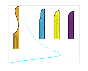
Figure 1. The moving contact-line problem in a channel geometry in a frame of reference that moves with the liquid. (a–c) The advancing contact-line problem. (d–f) The receding contact-line problem. In both cases, as the speed of the substrate,  $U^*$, increases, the system is first stable (a,d), before the system becomes transient at a critical speed $U^*_{{crit}}$ (b,e) and air entrainment (c) or thin-film formation (f) occurs. We denote the characteristic horizontal width of the fluid entrainment region in the advancing problem as $\hat {h}$ and the characteristic horizontal width of the thin film in the receding problem as $h_{{film}}$. The height of the interface, defined as the difference in heights of the left and right contact points, is denoted $Y$ (cf. (2.21)). (a) Stable. (b) Critical. (c) Fluid entrainment. (d) Stable. (e) Critical. ( f) Thin film.
The critical speed where the instability occurs is associated with a fold bifurcation in the steady solution structure (see e.g. Vandre, Carvalho & Kumar Reference Vandre, Carvalho and Kumar2013; Kamal et al. Reference Kamal, Sprittles, Snoeijer and Eggers2019), which divides the steady solutions between a stable branch and an unstable branch (as seen in figure 2a; see Kuznetsov (Reference Kuznetsov1998) for a detailed mathematical description). For parameter values ‘beyond the fold’ there are no (known) two-dimensional steady states and the system must become transient and/or three-dimensional. In our system, the appropriate non-dimensional parameter associated with the speed of the solid is the capillary number,  $Ca$ (see next section for a precise definition). Whilst analysis of the unstable branch of solutions (which exists for parameter values ‘below the fold’) can reveal important information about transient behaviour, the focus of theoretical studies has been mainly to calculate and characterise only the stable steady solutions immediately up to the critical speed (see e.g. Eggers Reference Eggers2005; Chan, Snoeijer & Eggers Reference Chan, Snoeijer and Eggers2012; Vandre et al. Reference Vandre, Carvalho and Kumar2013; Sprittles Reference Sprittles2015).

Figure 2. (a) A sketch of a typical fold bifurcation structure. A solution measure is plotted against a control parameter to form a solution curve. At a critical value, two branches – one stable (solid line) and one unstable (dashed line) – meet. The location of their intersection is known as a fold bifurcation. Beyond the critical value there are no (known) steady states. In our specific problem the control parameter is  $Ca$ and the solution measure is either the interface length or meniscus rise. (b) A generic two-dimensional phase plane for a parameter value less than the critical value with a stable state (an ‘attractor’ on the stable branch, see a), and a weakly unstable state (a ‘saddle-node’ on the unstable branch, see a). The unstable/stable manifolds of the saddle node are dashed/dotted respectively.
Interestingly, Chan et al. (Reference Chan, Snoeijer and Eggers2012) hypothesised that the set of unstable solutions represents, what they termed, ‘effective dynamics’, so that the unstable branch of the bifurcation curve guides time-dependent behaviour of the system. More specifically, when the capillary number is above its critical value ( $Ca>Ca_{{crit}}$), and the speed of the contact line is measured relative to that of the solid, time-dependent trajectories closely match those obtained from the unstable branch of the steady system, as confirmed experimentally in Delon et al. (Reference Delon, Fermigier, Snoeijer and Andreotti2007). Therefore, the unstable branch is not just an insignificant consequence of the fold bifurcation but provides unique insight into the system dynamics. Such an influence and importance of unstable states in fluid dynamics systems has been investigated in many different contexts, including shear flow (Eckhardt et al. Reference Eckhardt, Faisst, Schmiegel and Schneider2008), droplets (Gallino, Schneider & Gallaire Reference Gallino, Schneider and Gallaire2018), finite air bubbles (Keeler et al. Reference Keeler, Thompson, Lemoult, Juel and Hazel2019; Gaillard et al. Reference Gaillard, Keeler, Thompson, Hazel and Juel2020) and a slide-coating flow (Christodoulou & Scriven Reference Christodoulou and Scriven1988). Indeed, as shown in figure 2(b), where the phase plane is sketched for a generic system with a stable (‘attractor’) and weakly unstable (‘saddle-node’) state, the unstable state can act as a separator of dynamical outcomes; its stable manifold is a dividing ‘line’ and its unstable manifold connects to the stable state. In this article we adapt these ideas from dynamical systems theory to the moving-contact-line problem, for the first time, to reveal the role of the unstable solutions. We calculate the bifurcation structure and stability properties of the steady solutions and relate these to time-dependent calculations in the subcritical ( $Ca< Ca_{{crit}}$) and supercritical ( $Ca>Ca_{{crit}}$) regimes.
We now provide some important background on moving contact lines. It is well known that the classical ‘moving-contact-line paradox’, as described in Huh & Scriven (Reference Huh and Scriven1971), can be alleviated if there is slip near the contact point. Asymptotically, if this slip occurs in an inner region, as considered by Voinov (Reference Voinov1976) and Cox (Reference Cox1986), then bending of the interface occurs in an intermediate region where viscous effects can cause the liquid–fluid interface to curve sharply. In this formulation, it is often assumed that the intermediate region connects to an outer region where the interface retains its static meniscus shape. The possible asymptotic matching of these regions has critical consequences and provides insight into the bifurcation structure of the steady solution space. In a series of remarkable articles (Eggers Reference Eggers2004a,Reference Eggersb, Reference Eggers2005), it was shown, by solving a lubrication model for a liquid–vacuum system, how the curvature of the inner and outer regions can be asymptotically matched. For the advancing contact line this can be achieved for all values of  $Ca$, but for the receding contact line, the matching fails when $Ca$ is past some critical threshold, interpreted as (i.e. defining) $Ca_{{crit}}$. The bifurcation structure of the stable and unstable branches of the receding contact line was then fully described using matched asymptotics and bifurcation theory by Chan et al. (Reference Chan, Snoeijer and Eggers2012) for $Ca\ll 1$, and $Ca_{{crit}}$ was determined to occur at a fold bifurcation.
The aforementioned analysis has been extended to general liquid–fluid systems, where the viscosity of the fluid phase is considered non-zero (Chan et al. Reference Chan, Srivastava, Marchand, Andreotti, Biferale, Toschi and Snoeijer2013; Kamal et al. Reference Kamal, Sprittles, Snoeijer and Eggers2019; Chan et al. Reference Chan, Kamal, Snoeijer, Sprittles and Eggers2020) and also for the full Navier–Stokes equations (Vandre, Carvalho & Kumar Reference Vandre, Carvalho and Kumar2012; Vandre Reference Vandre2013; Vandre et al. Reference Vandre, Carvalho and Kumar2013). A key result from these studies is that, for the advancing contact line, the presence of viscosity fundamentally alters the bifurcation structure and a fold bifurcation appears at a finite  $Ca$. Vandre et al. (Reference Vandre, Carvalho and Kumar2013) showed that, physically, this fold bifurcation in the advancing contact-line problem occurs when the horizontal air-pressure gradient matches the strength of the capillary-stress gradient near the contact point. It was also demonstrated that using the lubrication model, in both phases, poorly predicts $Ca_{{crit}}$ when compared to the full Navier–Stokes equations for the advancing contact line (Vandre et al. Reference Vandre, Carvalho and Kumar2012; Vandre Reference Vandre2013; Vandre et al. Reference Vandre, Carvalho and Kumar2013). Other physical effects such as Marangoni flows, inertia, gravity and shear thinning/thickening were also found to preserve the fold bifurcation (Vandre et al. Reference Vandre, Carvalho and Kumar2013; Liu et al. Reference Liu, Vandre, Carvalho and Kumar2016a,Reference Liu, Vandre, Carvalho and Kumarb; Liu, Carvalho & Kumar Reference Liu, Carvalho and Kumar2017, Reference Liu, Carvalho and Kumar2019; Charitatos et al. Reference Charitatos, Suszynski, Carvalho and Kumar2020).
In the advancing case, the critical behaviour indicates the threshold at which fluid entrainment occurs where, experimentally, a three-dimensional saw-tooth pattern emerges as observed in a variety of different flow configurations, e.g. liquid films (Reysatt & Quéré Reference Reysatt and Quéré2006), drop impact (Thoroddsen et al. Reference Thoroddsen, Thoraval, Takehara and Etoh2012; Pack et al. Reference Pack, Kaneelil, Kim and Sun2018) and plate penetration in a liquid bath (He & Nagel Reference He and Nagel2019). In the receding case, however, the fold bifurcation marks the onset of thin-film deposition (Snoeijer et al. Reference Snoeijer, Delon, Andreotti and Fermigier2006, Reference Snoeijer, Ziegler, Andreotti, Fermigier and Eggers2008). Interestingly, despite the three-dimensional structures of air entrainment (He & Nagel Reference He and Nagel2019; He Reference He2020), two-dimensional models appear to accurately predict the transition point, an observation which is yet to be understood (see e.g. Vandre et al. Reference Vandre, Carvalho and Kumar2012; Sprittles Reference Sprittles2017; Liu et al. Reference Liu, Carvalho and Kumar2019). Transversal three-dimensional perturbations have been considered for the receding contact line (Snoeijer et al. Reference Snoeijer, Andreotti, Delon and Fermigier2007) and the advancing contact line (Vandre Reference Vandre2013), both using a lubrication model, but a stability analysis using the full hydrodynamics equations has not yet been conducted.
In this article, we develop a computational framework and methodology that can quantitatively determine the stability of dynamic contact lines. To do so, we use ideas from dynamical systems theory to understand the effect of the stable/unstable states on the transient dynamics, considering both advancing and receding contact lines. We emphasise that the methodology we describe here can easily be extended to include different physics, including the effects of inertia, gravity, different slip conditions on the moving plate and different models that account for a velocity-dependent contact angle. We choose to focus on understanding the qualitative transient behaviour, from a dynamical systems perspective, rather than attempting to include every physical effect in our model. Our analysis of two-phase contact-line stability focuses on steady-state solutions using a hybrid model; the liquid phase is modelled using the Navier–Stokes equations and the fluid phase is accurately modelled using a lubrication approximation (see Stay & Barocas Reference Stay and Barocas2003; Liu et al. Reference Liu, Vandre, Carvalho and Kumar2016a,Reference Liu, Vandre, Carvalho and Kumarb, Reference Liu, Carvalho and Kumar2017; Sprittles Reference Sprittles2017; Liu et al. Reference Liu, Carvalho and Kumar2019).
The structure of the article is as follows. In § 2 we discuss the hydrodynamic equations that describe the system. In § 3 we calculate the steady solution curves to determine the critical parameters associated with the loss of stability of the system. In addition, we perform a numerical linear stability analysis that reveals the significance of the unstable branch to the transient dynamics of the system. By treating the governing equations as a dynamical system we form a generalised eigenproblem that can be solved numerically to determine and quantify the stability of the solution branch. Next, in § 4, by solving a time-dependent initial value problem (IVP) numerically we are able to demonstrate that, far from having a passive role, the unstable branch represents, in the language of dynamical systems theory, the ‘basin boundary of attraction’ of the stable state. Furthermore, by examining the phase plane of the solution trajectory, we discover that the subsequent unsteady time evolution is intrinsically linked to the unstable branch and are able to confirm the prediction of Chan et al. (Reference Chan, Snoeijer and Eggers2012) that the receding contact line moves quasi-statically along the unstable branch. Viewing the trajectories through the lens of the phase plane allows us to understand if, and how, the system becomes transient when  $Ca< Ca_{{crit}}$ and also provides criteria that could potentially enable suppression of this instability. Finally, in § 5, we discuss the implications of these results and some possible future research.
2. Governing equations
We now discuss the hydrodynamic model and the assumptions that allow us to derive an accurate simplified hybrid model that is used in the calculations thereafter. The following discussion applies to both the advancing and receding contact lines, although the demonstrative figures only show the advancing contact line.
2.1. Full hydrodynamic model
Motivated by the system used in Vandre et al. (Reference Vandre, Carvalho and Kumar2012), which is representative of an experimental system, we consider two-dimensional flow between two parallel plates, as shown in figure 1. In the following discussion we denote dimensional quantities using an asterisk. Two fluids of viscosity  $\mu _{1,2}^*$, and density $\rho _{1,2}^*$, fill the channel bounded by two rigid plates which are separated by a fixed distance $H^*$; subscript 1 indicates the upper fluid (the fluid phase) and subscript 2 indicates the lower fluid (the liquid phase). In our system the left plate moves with constant speed in the $y$ direction $U^*$ and the right plate is stationary. For a receding contact line $U^*>0$ and an advancing contact line $U^*<0$. The fluid flow of each phase is governed by the two-dimensional Navier–Stokes equations. All speeds, lengths, pressures and times are scaled by $U^*$, $H^*$, $\mu _2^*U^*/H^*$ and $H^*/U^*$ respectively. Finally, the viscosity ratio, denoted $\chi$, is defined with respect to the liquid phase, i.e.
 \begin{equation} \chi = \mu_{1}^*/\mu_{2}^*, \end{equation}
and we assume that the upper fluid is less viscous, i.e.  $\chi < 1$.
As in previous studies (Sprittles & Shikhmurzaev Reference Sprittles and Shikhmurzaev2011a,Reference Sprittles and Shikhmurzaevb; Vandre et al. Reference Vandre, Carvalho and Kumar2012; Sprittles & Shikhmurzaev Reference Sprittles and Shikhmurzaev2013; Vandre et al. Reference Vandre, Carvalho and Kumar2013; Liu et al. Reference Liu, Vandre, Carvalho and Kumar2016a,Reference Liu, Vandre, Carvalho and Kumarb, Reference Liu, Carvalho and Kumar2017, Reference Liu, Carvalho and Kumar2019) we apply the Stokes-flow approximation so that the Reynolds number,  $Re = U^*H^*\rho _2^*/\mu _2^*$, is negligible and assumed zero; results in Vandre et al. (Reference Vandre, Carvalho and Kumar2013) show $Re$ can have an influence at sufficiently high values but it does not qualitatively alter the conclusions. We assume that gravitational effects are negligible throughout. The non-dimensional computational domain is shown in figure 3(c). The coordinate system is centred on the contact point between the two fluids and the left (moving) plate. The boundary corresponding to the left plate is denoted $\varGamma _1$, the right plate $\varGamma _2$, the bottom $\varGamma _3$, the free surface $\varGamma _4$ and the top $\varGamma _5$. The fluid and liquid domains are denoted by $\varOmega _1$ and $\varOmega _2$ respectively. The Stokes-flow equations for the fluid velocity, $\boldsymbol {u}_i = (u_i,v_i)$, and pressure, $p_i$, in each phase can be written as
 \begin{align} \chi \nabla^2\boldsymbol{u}_1 &= \boldsymbol{\nabla} p_1,\quad\boldsymbol{\nabla}\boldsymbol{\cdot}\boldsymbol{u}_1 = 0,\quad \boldsymbol{x}\in \varOmega_1\quad\text{(fluid)}, \end{align}
 \begin{align} \nabla^2\boldsymbol{u}_2 &= \boldsymbol{\nabla} p_2,\quad\boldsymbol{\nabla}\boldsymbol{\cdot}\boldsymbol{u}_2 = 0,\quad \boldsymbol{x}\in \varOmega_2\quad\text{(liquid)}. \end{align}
Figure 3. The computational domain for the hybrid and full models for an advancing contact line. The boundaries are denoted by  $\varGamma _i$ (labelled in c) with the origin centred on the contact line. (a) A typical streamline pattern for a steady solution in the hybrid model. (b) The computational domain for the hybrid model. In this model we solve for the velocity and pressure in the liquid domain, but only solve for the pressure of the fluid on the interface boundary, $\varGamma _4$. (c) The computational domain for the full model where the velocity and pressure fields are also solved in the fluid domain. (d) The vertical component of velocity along the moving plate, i.e. $\varGamma _1$. (e) The enlargement near the contact line shows the mesh refinement required to ensure that the flow field is sufficiently resolved.
On the left (moving) and right (stationary) plates,  $\varGamma _1$ and $\varGamma _2$ respectively, we implement a Navier slip condition written as
 \begin{align} \lambda ( \boldsymbol{\tau}_i \boldsymbol{\cdot} \boldsymbol{n}_{{p}})\boldsymbol{\cdot}\boldsymbol{t}_{{p}} &= (\boldsymbol{u}_{i} - \boldsymbol{U})\boldsymbol{\cdot} \boldsymbol{t}_{{p}},\quad\boldsymbol{x}\in\varGamma_{1},\quad i = 1,2, \end{align}
 \begin{align} \lambda ( \boldsymbol{\tau}_i \boldsymbol{\cdot} \boldsymbol{n}_{{p}})\boldsymbol{\cdot}\boldsymbol{t}_{{p}} &= \boldsymbol{u}_{i} \boldsymbol{\cdot} \boldsymbol{t}_{{p}},\quad\boldsymbol{x}\in\varGamma_{2},\quad i = 1,2, \end{align}
where  $\boldsymbol {n}_{{p}}$ and $\boldsymbol {t}_{{p}}$ are the vectors normal and tangential to each plate respectively, $\boldsymbol {U} = (0,U)$ is the non-dimensional speed of the (moving) left plate (where $U$, in our dimensionless system, is $\pm 1$, corresponding to the receding (+)/advancing (−) problem) and $\lambda$ is the non-dimensional slip length which, for simplicity, we assume to be the same in each phase (see Sprittles (Reference Sprittles2017) for potential extensions). We could choose different conditions that regularise the singularity at the contact line (Shikhmurzaev Reference Shikhmurzaev2006), but, assuming the actual contact angle is unchanged, the details of the solution (i.e. the value of $Ca_{{crit}}$) are more sensitive to values of the slip-length parameter that arises in these models (in our case $\lambda$) than the actual form of the model (Dussan Reference Dussan1976). Thus, we would expect the results we obtain to be qualitatively similar to those obtained for a different slip model, although such slip models are easy to implement, if required. We choose a moderate value of $\lambda = 0.1$, and although quantitative details, i.e. the values of $Ca_{{crit}}$ and other solution measures, will differ as we vary $\lambda$, we find that the transient behaviour and solution structure, as we describe later in the article, are qualitatively the same (cf. figure 7).
We choose to implement a Navier slip condition on the stationary plate for consistency and to ensure that the contact point on the stationary plate is allowed to move. However, we could fix  $\boldsymbol {u}_i = 0$ on $\varGamma _2$ and get similar results (see e.g. Vandre et al. Reference Vandre, Carvalho and Kumar2013; Liu et al. Reference Liu, Carvalho and Kumar2017) which corresponds to a pinned contact line. We also implement a no-penetration condition on each plate, i.e.
 \begin{equation} \boldsymbol{u}_i\boldsymbol{\cdot} \boldsymbol{n}_{{p}} = 0,\quad\boldsymbol{x}\in\varGamma_1\cup\varGamma_2,\quad i = 1,2. \end{equation}
The stress tensor in each phase  $\boldsymbol {\tau }_i$ is defined as
 \begin{equation} \boldsymbol{\tau}_i ={-}p_i\boldsymbol{I} + \delta_i(\boldsymbol{\nabla} \boldsymbol{u}_i + (\boldsymbol{\nabla}\boldsymbol{u}_i)^{\rm T}), \end{equation}
where  $\boldsymbol {I}$ is the identity matrix and $\delta _1 = \chi, \delta _2 = 1$. We denote the unknown position of the interface, $\varGamma _4$, as $\boldsymbol {r} = (x_s,y_s)$ (see figure 3b) and assume a constant surface tension, $\gamma ^*$, so that the dynamic boundary condition can be written as
 \begin{equation} \boldsymbol{\tau}_1\boldsymbol{\cdot}\boldsymbol{n} - \boldsymbol{\tau}_2\boldsymbol{\cdot}\boldsymbol{n} = \frac{1}{Ca}\kappa \boldsymbol{n},\quad\boldsymbol{x}\in\varGamma_{4}, \end{equation}
where  $\boldsymbol {n}$ is the normal of the interface pointing towards the fluid phase (see figure 3b), $\kappa = \boldsymbol {\nabla }\boldsymbol {\cdot }\boldsymbol {n}$ is the curvature of the interface and $Ca = \mu _2^*|U|/\gamma ^*$ is the capillary number. In addition to (2.8), we impose a kinematic condition on $\varGamma _4$, written as
 \begin{equation} \frac{\partial \boldsymbol{r}}{\partial t}\boldsymbol{\cdot}\boldsymbol{n} = \boldsymbol{u}\boldsymbol{\cdot}\boldsymbol{n}, \quad\boldsymbol{x}\in\varGamma_{4}. \end{equation}
We have to specify the angle that the interface makes on the left and right plates. These angles can be allowed to vary with the capillary number, slip length or other quantities but we choose the simplest approach and take these to be constant values, i.e.
 $$\begin{gather} \theta = \theta_1,\quad \text{on}\ \varGamma_1\cap\varGamma_4, \end{gather}$$
 $$\begin{gather}\theta = \theta_2,\quad \text{on}\ \varGamma_2\cap\varGamma_4. \end{gather}$$
It is straightforward to replace these conditions with equations involving  $Ca$ and other quantities, but this is not the focus of this article.
Finally, we implement fully developed flow conditions on the inflow and outflow boundaries:
 \begin{equation} \boldsymbol{u}_i\boldsymbol{\cdot}\boldsymbol{t}_{{inflow}} = 0,\,\boldsymbol{x}\in\varGamma_{3}\cup\varGamma_{5}, \end{equation}
where  $\boldsymbol {t}_{{inflow}} = (1,0)^{\rm T}$, alongside a pressure drop across the domain so that
 $$\begin{gather} p_1 = 0,\,\boldsymbol{x}\in\varGamma_{5}, \end{gather}$$
 $$\begin{gather}p_2 = p_{{out}},\,\boldsymbol{x}\in\varGamma_{3}. \end{gather}$$
 The full hydrodynamic system is defined in (2.2)–(2.14) with the following infinite-dimensional state vector (denoted  $\boldsymbol {w}$) of unknowns:
 \begin{equation} \boldsymbol{w} = [\boldsymbol{u}_1,\boldsymbol{u}_2,p_1,p_2,\boldsymbol{r}]^{\rm T}. \end{equation}
It is worth noting that we model the effect of varying the speed of the plate by varying  $Ca$ and that the non-dimensional slip length, $\lambda$, can be varied to investigate changes in physical channel width. Finally, as our primary interest is in understanding the transient behaviour, for simplicity, we set $\theta _1 = \theta _2 = {\rm \pi}/2$ in all simulations. Therefore we have a set of control parameters,
 \begin{equation} Ca,\lambda,\chi,p_{{out}}, \end{equation}
2.2. Hybrid model
The computational cost of the full model can be significantly reduced by solving the thin-film equations where they are valid (Oron, Davis & Bankoff Reference Oron, Davis and Bankoff1997; Jacqmin Reference Jacqmin2004; Sbragaglia, Sugiyama & Biferale Reference Sbragaglia, Sugiyama and Biferale2008), leading to a hybrid model (see Stay & Barocas Reference Stay and Barocas2003; Liu et al. Reference Liu, Vandre, Carvalho and Kumar2016a,Reference Liu, Vandre, Carvalho and Kumarb, Reference Liu, Carvalho and Kumar2017, Reference Liu, Carvalho and Kumar2019; Charitatos et al. Reference Charitatos, Suszynski, Carvalho and Kumar2020) which approximately halves the complexity of the problem, as unknowns in the fluid phase are only computed on the interface. The difference of our approach from previous implementations is that our hybrid model takes into account time dependence so that stability can be probed and IVP calculations can be performed. A key assumption is that a typical horizontal distance in the fluid phase, when air entrainment occurs, is small when compared to the vertical height of the meniscus (i.e.  $\hat {h}\ll Y$ in figure 1) so that the flow is approximately parallel, i.e. the cross-stream component of $\boldsymbol {u}_1$ is small. The full derivation is discussed in Appendix A and the computational domain is shown in figure 3(b).
The effect of this reduction in the fluid phase is to replace a full two-dimensional description, given in (2.2), by a one-dimensional equation for the fluid pressure,  $p_1$, on the interface only. This equation can be stated as
 \begin{equation} \frac{\partial \boldsymbol{r}}{\partial t}\boldsymbol{\cdot}\boldsymbol{n} \pm \frac{1}{\chi}\frac{\partial Q_1}{\partial s} = 0,\quad Q_1 = \frac{1}{6}\frac{\partial p_1}{\partial s}h^3 + \frac{1}{2}Ah^2 + Bh, \end{equation}
where  $h$ is the horizontal distance (i.e. $x_s$) from the left plate to the interface (see figure 3), $Q_1$ is the flux and the constants $A$ and $B$ are functions of $\chi,\lambda$ and $\boldsymbol {u}_2$ and are given in Appendix A. The $\pm$ sign is used for the advancing ( $+$)/receding ( $-$) contact line. The fluid phase is coupled to the liquid phase through the applied traction given in (A6). We now have a system of partial differential equations (PDEs) described by (2.3)–(2.14) and (2.17a,b) with the infinite-dimensional state vector of unknowns:
 \begin{equation} \boldsymbol{w} = [\boldsymbol{u}_2,p_2,p_1(\boldsymbol{r}),\boldsymbol{r}]^{\rm T}. \end{equation}
The hybrid model has been extensively validated for steady advancing contact-line problems against the full system and experiment (Liu et al. Reference Liu, Vandre, Carvalho and Kumar2016b, Reference Liu, Carvalho and Kumar2019). We validate the time-dependent hybrid model by comparing to the full hydrodynamic model in Appendix A. Finally we note that this approach is strictly only valid for the advancing contact-line problem but, as shown later, the receding contact-line problem is effectively a one-phase problem (cf. figure 7), and implementing the hybrid model for a receding contact line does not significantly change the value of  $Ca_{{crit}}$ (Appendix A).
2.3. System parameters and integral measures
We now describe additional system parameters and measures that will be useful in computing and describing the steady and time-dependent solutions. The pressure at the outflow boundary,  $p_{{out}}$, is determined implicitly by an integral volume constraint acting on the liquid phase, i.e.
 \begin{equation} \iint_{{\varOmega_2}}\,{\rm d}V = V, \end{equation}
where  $V$ is the volume of the liquid domain (corresponding to the area of the computational domain). In our numerical calculations the positions of the contact points on the moving and stationary plates are both allowed to move so that (2.19) can be satisfied. For ease of presentation, we post-process and rescale the solution so that the origin is always at the contact point of the moving plate. In the calculations that follow we choose a value of $V$ which is large enough for fully developed flow to occur near the outflow boundary, $\varGamma _1$. After careful experimentation we find that the solutions are independent of values of $V\geq 5$ that we choose.
For a fixed set of parameter values, as defined in (2.16), we calculate steady solution curves by setting the time derivatives in the governing equations to zero and then solving the resulting steady system. As we vary  $Ca$, and then subsequently calculate a solution, a solution curve will be traced and a fold bifurcation will occur at the critical value of the capillary number, denoted $Ca_{{crit}}$. Whilst it is possible to trace a solution branch around the fold numerically by a pseudo-arclength continuation method (see e.g. Doedel Reference Doedel2007), we implement an alternative, bespoke approach. We expect the interface length, $L$, to increase monotonically as the curve is traced out around the fold and therefore it is a suitable candidate for a continuation parameter that allows us to calculate solutions smoothly around the fold. To achieve this, we let $Ca$ become an unknown parameter that is determined implicitly by setting the total length of the interface, i.e.
 \begin{equation} \int_{\varGamma_{4}}\,{\rm d}s = L. \end{equation}
This approach enables us to trace solution curves around the fold by incrementally increasing  $L$ and solving the system of equations, with $Ca$ effectively determined by (2.20). We also emphasise that (2.19) and (2.20) are only implemented in steady calculations; the former constraint is unnecessary in time-dependent calculations as the second equation in (2.3) ensures volume is conserved, whilst the latter constraint is used as a means of tracing the solution curve.
Finally, when describing the steady solutions and time-dependent solutions we use the meniscus rise (more specifically, the vertical distance between the two contact lines) defined as
 \begin{equation} Y(t) = |y_s(s=L) - y_s(s=0)| \end{equation}
as a convenient solution measure (as previously considered, for example, in Kamal et al. (Reference Kamal, Sprittles, Snoeijer and Eggers2019); see figure 3 (in this article) for reference).
2.4. Numerical method
The governing equations are solved using the finite-element method from within the open-source oomph-lib object-orientated multi-physics library (Heil & Hazel Reference Heil and Hazel2006). The structure and implementation of our equations follow that of Sprittles & Shikhmurzaev (Reference Sprittles and Shikhmurzaev2013). Following multiplication of the equations by a test function,  $\psi$, and then an integration over the domain, the boundary integrals that result from integration by parts require the traction to be specified on each of the boundaries. The dynamic condition, (2.8), and the Navier slip condition, (2.5), therefore can be implemented as a natural condition by these boundary integrals.
Special care has to be taken at the contact point. In other studies (Vandre et al. Reference Vandre, Carvalho and Kumar2012, Reference Vandre, Carvalho and Kumar2013; Liu et al. Reference Liu, Vandre, Carvalho and Kumar2016a,Reference Liu, Vandre, Carvalho and Kumarb, Reference Liu, Carvalho and Kumar2017, Reference Liu, Carvalho and Kumar2019) the contact angle is imposed as an essential boundary condition at the expense of solving a component of the momentum equations at the contact point. We adopt the approach of Sprittles & Shikhmurzaev (Reference Sprittles and Shikhmurzaev2013) and impose the contact angle as a natural boundary condition on both the intersection of the free surface with the left plate ( $\varGamma _1$) and the symmetry plate ( $\varGamma _2$). We therefore introduce a field of Lagrange multiplier unknowns on $\varGamma _1$ and $\varGamma _2$ which are determined from the weak form of the no-penetration condition, (2.6). We refer the reader to Sprittles & Shikhmurzaev (Reference Sprittles and Shikhmurzaev2013) for a detailed description of this implementation (we adopt approach (B) in their nomenclature).
As is standard, the fluid velocities are interpolated using bi-quadratic shape functions and the pressure using linear continuous shape functions with Taylor–Hood triangular elements. We choose to mesh the liquid domain using an unstructured triangular grid (see figure 3b,c). The mesh is considered to be a fictitious pseudo-solid with the position of the nodes coming as part of the solution. The weak form of the kinematic condition, (2.9), is imposed as an essential condition and determines a field of Lagrange multipliers (not to be confused with the Lagrange multipliers in the previous paragraph) that act on the solid deformation equations which in turn determines the shape of the unknown interface,  $\boldsymbol {r}$; see Sackinger, Schunk & Rao (Reference Sackinger, Schunk and Rao1996) for more details. We note that this approach results in a large system of equations which is disadvantageous, but it allows for the interface to become highly deformed, as well as naturally handling time-dependent flow (where the domain could significantly change shape; cf. figure 1), which is difficult to achieve if the mesh is structured.
To solve the hybrid equation, (2.17a,b), it is convenient to introduce two fields of unknowns on the fluid interface, the pressure  $p_1$ and flux $Q_1$, interpolated using quadratic shape functions. We solve two equations in their weak form:
 \begin{equation} \int_{S}(Q_1 - Q_{C})\psi\,{\rm d}S = 0,\quad Q_{C} = \frac{1}{\chi}\left(Ah + \frac{1}{2}Bh^2 + \frac{1}{6}h^3\frac{\partial p}{\partial s}\right) \end{equation}
and
 \begin{equation} \int_{S} \left(\frac{\partial \boldsymbol{r}}{\partial t}\boldsymbol{\cdot}\boldsymbol{n} \pm \frac{\partial Q_1}{\partial s}\right)\psi\,{\rm d}s = 0. \end{equation}
Equation (2.22a,b) projects the flux from the lubrication equation onto the finite-element space and then (2.23) ensures mass is conserved in the fluid phase.
The resulting discretised equations are solved with Newton's method using the SuperLu numerical algebra package (Li Reference Li2005). For time-dependent calculations the solution is updated in time using a backwards-difference second-order Euler method (BDF2). A typical streamline pattern is shown in figure 3(a).
Around the contact line the interface becomes highly deformed due to viscous bending and the pressure and velocity gradients are large (see figure 3d,e). In steady calculations, as  $Ca\to Ca_{{crit}}$, we expect the number of elements required in the vicinity of the contact line to increase to ensure a smooth converged solution. We re-mesh the domain according to a ZZ error estimator (Zienkiewicz & Zhu Reference Zienkiewicz and Zhu1992), which measures the discontinuity of strain-rate gradients between adjacent elements and interprets this as a measure for the local error. Typically we set a minimum error as $10^{-6}$ and a maximum error $10^{-3}$, so that elements with error above this range get refined and those with error below this range get unrefined. We allow element sizes from $10^{-12}$ to $10^{-2}$ to accommodate these error estimates. We do not adapt the mesh at each calculation; rather we adapt the mesh based on the condition that
 \begin{equation} |\theta_1 - \theta_c| < 1.0^{{\circ}},\quad \theta_c = \text{atan} ((y_2 - y_1)/(x_2 - x_1)), \end{equation}
where  $\theta _c$ is the computed angle based on $(x_1,y_1)$ and $(x_2,y_2)$, the coordinates of the nodes on $\varGamma _4$ directly at the contact line and immediately adjacent, respectively. The number of elements and their sizes are highly dependent on $\lambda$ and $Ca$. As an illustrative example, for steady solutions at $\lambda = 0.1$, $\chi =0.1$ and $V=5$, the resulting mesh has ${\sim}10^3$ triangular elements and ${\sim}10^5$ discretised unknowns at $Ca = Ca_{{crit}}$.
3. Linear stability analysis
We now present the stability algorithm and results. Rather than perform a standard normal modes reduction to the Orr–Somerfeld equations (see e.g. Severtson & Aidun Reference Severtson and Aidun1996), we take a more general approach that determines the modes as part of the solution. The analysis below is independent of the model, and although the results we present are from the hybrid model, these results also follow from the full model.
In both cases the PDE system can be written as
 \begin{equation} \mathcal{R}(\dot{\boldsymbol{w}},\boldsymbol{w}) = 0, \end{equation}
where  $\mathcal {R}$ is a nonlinear operator and $\boldsymbol {w}(t)$ represents a state of the system at time $t$, given as a vector of all the unknowns (either (2.15) or (2.18)). The time derivatives, $\dot {\boldsymbol {w}}$, appear in linear combinations in our system so we can decompose $\mathcal {R}$ into a linear mass operator, $\mathcal {M}$, that operates on the time derivatives in the problem and a nonlinear operator, $\mathcal {F}$, that operates on the spatial derivatives in the problem so that (3.1) becomes
 \begin{equation} \mathcal{R}(\dot{\boldsymbol{w}},\boldsymbol{w}) \equiv \mathcal{M}(\dot{\boldsymbol{w}}) + \mathcal{F}(\boldsymbol{w}) = 0. \end{equation}
 To proceed we write the state of the system,  $\boldsymbol {w}$, as a perturbation expansion, i.e.
 \begin{equation} \boldsymbol{w} = \boldsymbol{w}_{{\star}} + \varepsilon \text{e}^{\sigma t}\boldsymbol{g} + O(\varepsilon^2), \end{equation}
where  $\boldsymbol {w}_{\star }$ is a base state only dependent on spatial variables, $\varepsilon \ll 1$ is a small parameter, $\boldsymbol {g}$ is an eigenmode that is dependent on spatial variables only and $\sigma$ is the growth rate of the perturbation. The expansion in (3.3) represents a general class of perturbations that satisfy the boundary conditions of the problem and are in-plane perturbations; we are not extending to the third dimension, a problem we will discuss later.
Substituting (3.3) into (3.2) gives a series of problems that have to be solved at each order of  $\varepsilon$. At leading order we have
 \begin{equation} \mathcal{F}(\boldsymbol{w}_{{\star}}) = 0. \end{equation}
The solution,  $\boldsymbol {w}_{\star }$, is the steady state of the system. At first order we solve
 \begin{equation} \left[\sigma\mathcal{M}(\boldsymbol{w}_{{\star}}) + \mathcal{J}(\boldsymbol{w}_{{\star}})\right]\boldsymbol{g} = 0, \end{equation}
where  $\mathcal {J}(\boldsymbol {w}_{\star })$ is the functional derivative of the nonlinear operator $\mathcal {F}$ applied at the steady state $\boldsymbol {w}=\boldsymbol {w}_{\star }$. Equation (3.5) is a generalised eigenvalue problem that can be solved to find $\boldsymbol {g}$ and $\sigma$. The eigenspectrum of $\sigma$ determines the stability of the steady solutions. If at least one of the spectrum of $\sigma$ has a positive real part then the steady state is linearly unstable. Conversely if the entire spectrum lies in the left half of the complex plane then the solution is linearly stable. In general there will be an infinite number of these eigenmodes and thus we can write the linearised solution as
 \begin{equation} \boldsymbol{w}_{{lin}}(t) = \boldsymbol{w}_{{\star}} + \sum_{n=1}^{\infty}a_n\boldsymbol{g}_n\text{e}^{\sigma_nt} + \text{c.c.}, \end{equation}
where c.c. denotes the complex conjugate and  $a_n$ are arbitrary constants set by the initial conditions. When the system becomes discretised, the operators $\mathcal {M}$ and $\mathcal {J}$ are represented by the mass matrix and Jacobian matrix, respectively. The mass-matrix representation of $\mathcal {M}$ is highly rank deficient as the only time derivatives occur at the fluid–liquid interface and special care has to be taken to ensure that the solution to (3.5) has converged. We use the Anasazi linear algebra library which is an iterative eigensolver that can solve highly rank-deficient eigenproblems (Heroux et al. Reference Heroux2003). As the spectrum has an infinite number of eigenvalues, the discretised spectrum will have a finite number of eigenvalues, proportional to the number of unknowns in the problem. We find a small subset of eigenvalues which have the largest real part as these will be the modes visible in the transient dynamics; large negative eigenvalues correspond to eigenmodes that decay very rapidly. We validate the calculations using a simplified lubrication model and present this in Appendix B.
3.1. Stability of the solution branches
We now discuss the bifurcation structure and the corresponding stability results of the advancing and receding dynamic contact-line problems. Figure 4 shows the bifurcation structures in a typical advancing case (figure 4a:  $\chi = 0.1, \lambda = 0.1$) and receding case (figure 4b: $\chi = 0.0, \lambda = 0.1$). Notably, our focus here is on providing insight into the stability structure, rather than necessarily probing the precise values from experimental analyses, where the slip length could be far smaller and therefore typically require more computational resources. Previous works (Vandre et al. Reference Vandre, Carvalho and Kumar2012) have shown that whilst changes in slip length can have a weak effect on $Ca_{{crit}}$, they do not qualitatively alter the physical mechanisms at play (similarly for smaller viscosity ratios, e.g. with a glycerol–air system).

Figure 4. Solution curves for the advancing (a) and receding (b) contact lines. The values of the control parameters are  $\chi = 0.1$ (a) and $0$ (b) and $\lambda = 0.1$ for both panels. Individual solutions are labelled on the curve and correspond to the inset panels with the same label. The solid/dashed lines sections of the curve are the stable/unstable branches, respectively. The smaller insets show the eigenspectra for the $\boldsymbol {A}_{1}/\boldsymbol {R}_{1}$ and $\boldsymbol {A}_{2}/\boldsymbol {R}_{2}$ solutions and at the fold. Solutions $\boldsymbol {A}_{3}/\boldsymbol {R}_{3}$ are the solutions where the inflection point on the interface first becomes parallel to the plate, i.e. when ${\rm d}\kern0.7pt x_s/{\rm d}y_s = 0$. In (a), $\boldsymbol {A}_{4}$ is the solution just before the numerical calculations cease to converge. In (b), $\boldsymbol {R}_{4}$ is the solution where the interface starts to ‘overhang’ the right plate. The top-left inset in (b) shows the bifurcation curve for larger $Y$.
$Y$.
The solution curves are shown in the  $(Ca,Y)$ projection of the solution space (see (2.21) for a definition of $Y$). The markers on the curve indicate specific solutions which are shown in the inset panels labelled $\boldsymbol {A}_{1}$– $\boldsymbol {A}_{4}$ for the advancing contact line, and $\boldsymbol {R}_{1}$– $\boldsymbol {R}_{4}$ for the receding contact line. In both the advancing and receding cases, as $Y$ increases, the solution curve experiences a fold which separates the lower branch and upper branch. The eigenspectra are real and at the fold a single eigenvalue crosses the imaginary axis, as expected. The eigenspectra also indicate that the $\boldsymbol {A}_{1}/\boldsymbol {R}_{1}$ states (all eigenvalues in the left-hand Argand plane) are ‘attractors’ of the system and $\boldsymbol {A}_{2}/\boldsymbol {R}_{2}$ states (a single eigenvalue in the right-hand Argand plane, akin to a ‘saddle-node’ state in a two-dimensional dynamical system) are weakly unstable, as seen in figure 2(b), thus numerically confirming that the lower branch is stable (solid curve) and the upper branch is unstable (dashed curve).
The interface has an inflection point near the contact point. We measure the angle at the interface inflection point (to the downwards vertical) and, as is common, define this as  $\theta _{{app}}$; the apparent contact angle (Vandre et al. Reference Vandre, Carvalho and Kumar2012; Liu et al. Reference Liu, Vandre, Carvalho and Kumar2016b). Notably, as can be seen from solutions $\boldsymbol {A}_{1},\boldsymbol {A}_{2}$ and $\boldsymbol {R}_{1},\boldsymbol {R}_{2}$ in figure 4, $\theta _{{app}}<180^\circ$ not only on the stable branch, but also immediately after the fold on the unstable branch. This is consistent with the asymptotic results of Eggers (Reference Eggers2004a), who shows that the solution at $Ca_{{crit}}$ has $\theta _{{app}} \to 180^\circ$ as $\lambda \to 0$. Consequently, for given $\lambda > 0$ we would expect to find that $\theta _{{app}} < 180^\circ$ at $Ca_{{crit}}$. These findings are consistent with Sbragaglia et al. (Reference Sbragaglia, Sugiyama and Biferale2008).
Further up the unstable branch, see  $\boldsymbol {A}_{3},\boldsymbol {A}_{4}$ and $\boldsymbol {R}_{3},\boldsymbol {R}_{4}$ in figure 4, $\theta _{{app}} = 180^{\circ }$ and the interface develops a stationary point (i.e. ${\rm d}\kern0.7pt x_s/{\rm d}y_s = 0$). In the advancing case, the solution curve terminates when the interface touches the right plate and effectively appears to ‘pinch off’ off the fluid domain; see $\boldsymbol {A}_{4}$. For the receding case, the calculations stop when the size of the computational domain no longer allows a converged solution.
The steady-solution curves of the advancing and receding contact-line problems, although treated separately in figure 4, are actually two halves of the same solution space. Figure 5 shows the connection for  $\lambda = 0.1,\chi = 0\text { and }0.1$, where the signed meniscus rise, $y_s(s=L) - y_s(s=0)$, is plotted against $Ca\times U$, where $U=\pm 1$ with $\pm$ corresponding to the receding ( $+$)/advancing ( $-$) problem. In this projection the advancing and receding curves occupy the second and fourth quadrants, respectively, and the location of the respective folds in each quadrant highlights that the advancing contact line only becomes unstable if $\chi \neq 0$, in which case $Ca_{{crit,rec}} < Ca_{{crit,adv}}$ (Marchand et al. Reference Marchand, Chan, Snoeijer and Andreotti2012; Chan et al. Reference Chan, Srivastava, Marchand, Andreotti, Biferale, Toschi and Snoeijer2013) and that, in general, $Ca_{{adv,crit}}$ and $Ca_{{rec,crit}}$ increase as $\chi \to 0$.

Figure 5. The advancing and receding steady solution curves for  $\lambda = 0.1$ and $\chi = 0$ (red curves), $\chi = 0.1$ (blue curves). The horizontal axis is $Ca$ scaled by $U=\pm 1$ and the vertical axis is $y_s(s=L) - y_s(s=0)$, i.e. the signed version of $Y$. The critical $Ca$ for each problem is denoted by a dotted line. The two problems are connected through the origin.
Finally, we note that in both cases the solution curve does not experience additional bifurcations as  $Y$ increases along the unstable branch. For a system where gravity is included it is known that within the lubrication approximation, the solution curve (for the receding contact line, at least) oscillates around a fixed value of $Ca = Ca^*$ (see Chan et al. Reference Chan, Snoeijer and Eggers2012), experiencing multiple saddle-node bifurcations as $Y\to \infty$. Preliminary calculations show that, if gravity is included, the oscillations are also present in the advancing/receding hybrid system, although, for brevity, we do not show the results here.
3.2. Physical interpretation of the bifurcation
As discussed in Vandre et al. (Reference Vandre, Carvalho and Kumar2013) for the advancing contact line, the fold occurs when the fluid-pressure gradients (fluid 1) are comparable to the capillary-stress gradients (see Vandre Reference Vandre2013) near the contact line, i.e. when
 \begin{equation} \frac{\partial p_1}{\partial s} \sim \frac{1}{Ca}\frac{\partial \kappa}{\partial s}. \end{equation}
This is because as  $Ca\to Ca_{{crit}}$ the air-pressure gradients near the contact line will increase as the system seeks to ‘pump’ air out of the region near the contact line to maintain a steady state. Eventually these air-pressure gradients will exceed the capillary-stress gradients and the system will be unable to maintain a stable steady equilibrium. Figure 6 shows the evolution of the quantities on either side of (3.7) calculated at the inflection point for the advancing case. Here, one can see that the air-pressure and capillary-stress gradients balance close to $Ca_{{crit}}$, as seen by the intersection of the curves, which confirms the ideas of Vandre et al. (Reference Vandre, Carvalho and Kumar2013).

Figure 6. Comparison of the air-pressure gradient and the capillary-stress gradient for the steady solutions at the inflection point (IP) on the interface for the advancing contact-line problem. Parameter values are  $\chi =0.1,\lambda = 0.1$.
3.3. Fold tracking
We can take advantage of the fact that at the fold bifurcation the leading eigenvalue crosses the imaginary axis to develop an algorithm for finding  $Ca_{{crit}}$. We augment the system with the additional constraint
 \begin{equation} \mathrm{Re}(\sigma_1) = 0, \end{equation}
and let another control parameter come as part of the solution. It is convenient to let the interface length,  $L$, be determined by (3.8) so we are able to track the evolution of $Ca_{{crit}}$ as another parameter, the viscosity ratio $\chi$, for example, is varied. This is a robust way of tracking the fold without having to recalculate the solution curve for every set of parameters, as previously considered in Kamal et al. (Reference Kamal, Sprittles, Snoeijer and Eggers2019) and Vandre et al. (Reference Vandre, Carvalho and Kumar2012).
If we vary  $\chi$ and calculate $Ca_{{crit}}$ we observe that the curve of the loci of $Ca_{{crit}}$ does not itself experience any bifurcation, as seen in figure 7(a,b). In addition, we observe that the bifurcation structure also remains intact when the slip length, $\lambda$, is varied (see figure 7c) . In fact, we note that the value of $Ca_{{crit}}$ only changes relatively weakly as $\lambda$ changes from $O(1)$ to $O(10^{-4})$. Therefore we expect the dynamics to be qualitatively similar (from a dynamical systems perspective) regardless of the slip length and provided $\chi \neq 0$.

Figure 7. The evolution of the fold, and hence  $Ca_{{crit}}$, as the relative viscosity $\chi$ (a,b) and the slip length $\lambda$ (c) are varied. (a) The advancing contact line, $\lambda = 0.1$. As $\chi \to 0$, $Ca_{{crit}}\to \infty$ so that the fold in the bifurcation structure ceases to exist. The inset shows the generic bifurcation structure in the $\chi =0$ and $\chi \neq 0$ cases. In the former case there is always a stable solution for the system to be attracted to. (b) The receding contact line, $\lambda = 0.1$. The fold exists for all viscosity ratios. For a given $\chi$ the bifurcation structure is shown in the inset. (c) Variation of $Ca_{{crit}}$ as $\lambda$ is varied for the advancing and receding problem (different colours) with $\chi = 0.1$.
An important observation is that the advancing and receding cases differ significantly as  $\chi \to 0$. For the advancing case, $Ca_{{crit}}\to \infty$ in this limit, whilst for the receding case it tends to a finite value. This indicates that the viscosity of the fluid phase has to be taken into account for the advancing contact line in order to describe the bifurcation structure. This feature has been identified before, in driven liquid filaments (Ledesma-Aguilar et al. Reference Ledesma-Aguilar, Nistal, Hernández-Machado and Pagonabarraga2011) and in plate-plunging experiments (Marchand et al. Reference Marchand, Chan, Snoeijer and Andreotti2012). In contrast the receding contact line is essentially a one-phase problem, and the qualitative features of the bifurcation structure are the same regardless of the viscosity of the fluid.
3.4. Eigenmode perturbations
We now discuss the nature of the eigenmodes resulting from the stability analysis. The modes corresponding to the three leading eigenvalues of the unstable branch, i.e.  $\sigma _1,\sigma _2\text { and }\sigma _3$, are shown in figure 8. These eigenmodes correspond to the base states $\boldsymbol {w}_{\star } = \boldsymbol {A}_2,\boldsymbol {R}_2$ in figure 4. In this figure the dotted profile indicates the steady interface shape and the coloured lines indicate the shape of the interface when it is perturbed by a single eigenmode, i.e.
 \begin{equation} \boldsymbol{w} = \boldsymbol{w}_{{\star}} \pm \rho \boldsymbol{g}_i,\quad i = 1,2,3. \end{equation}
The dashed/solid curves correspond to the  $+/-$ sign, respectively. The amplitude of the perturbation, $\rho$, is constrained so that the meniscus rise of the perturbation is no more than 10 % of the rise of the steady solution. Each successive mode intersects the steady interface at precisely one more location, in similarity to the form of the (sinusoidal) eigenmodes in a related lubrication model (see figure 20). Thus, the effect of adding higher-order eigenmodes to the steady state is to add extra corrugations to the interface and increase the overall length of the interface.

Figure 8. The eigenmodes of the unstable branch. The steady profile is shown as the dotted line. (a–c) The leading eigenmodes,  $\boldsymbol {g}_1,\boldsymbol {g}_2,\boldsymbol {g}_3$, corresponding to the advancing $\boldsymbol {w}_{\star } = \boldsymbol {A}_2$ ( $Ca=0.873,\chi =0.1$) solution in figure 4(a). (d–f) The leading eigenmodes corresponding to the receding $\boldsymbol {w}_{\star } = \boldsymbol {R}_2$ ( $Ca=0.3,\chi =0$) solution in figure 4(b). In each case the eigenmodes cross the steady interface in successively more locations. The slip length is $\lambda = 0.1$.
Concentrating on the leading eigenmode alone, the action of adding a multiple of  $\boldsymbol {g}_1$ to a steady solution, i.e. using (3.9), stretches/shrinks the interface according to the $\pm$ sign with no additional corrugations. Figure 9(a) shows the stable $\boldsymbol {A}_{1}$ and unstable $\boldsymbol {A}_{2}$ states with solid lines and the perturbation from the $\boldsymbol {A}_{1}$ state using (3.9) and $i=1$ with dotted lines. This figure demonstrates that we can continuously ‘stretch’ the nonlinear stable state by increasing the strength of the perturbation, $\rho$, and can eventually achieve an interface with an identical value of $Y$ to the unstable steady state and remarkably similar profile. This will have consequences, as discussed in the next section. We can also continuously deform the unstable branch in the same manner to match the interface of the stable branch. Therefore, we denote perturbations using the leading eigenmode only in (3.9) as ‘stretch’ perturbations.

Figure 9. Perturbations of the advancing  $\boldsymbol {w}_{\star }=\boldsymbol {A}_1$ state. (a) ‘Stretch’ perturbations. The lower solid curve is the stable interface and the upper solid curve is the unstable interface. The dotted curves are different strength perturbations of the stable state according to (3.9) with $i=1$. The dashed curve corresponds to the perturbation which results in an identical value of $Y$ as the $\boldsymbol {A}_2$ state. (b) ‘Corrugation’ perturbations. The coloured curves are different strength perturbations of the stable state according to (3.10) for a fixed value of $\rho$ and increasing $N$ and the shaded region represents the nonlinear $\boldsymbol {A}_{1}$ steady solution. Parameter values are $Ca = 0.873,\chi =0.1,\lambda = 0.1$.
In a physical experiment, perturbations will naturally emerge from the presence of ‘noise’ in the system causing fluctuations of the interface and contact line. We will take advantage of the stability analysis and mimic this ‘noise’ by using the higher-order eigenmodes in the perturbation, i.e.
 \begin{equation} \boldsymbol{w} = \boldsymbol{w}_{{\star}} + \sum_{i=1}^{N}\rho_i\boldsymbol{g}_i, \end{equation}
where for the purpose of simple illustration we choose the amplitude coefficients,  $\rho _i$, to be equal. Figure 9(b) shows the perturbed interface as the value of $N$ increases from 1 to 10, which demonstrates that by increasing the value of $N$ we are able to perturb the nonlinear steady interface with increasingly more corrugations or ‘noise’ in a systematic manner and hence be able to isolate specific geometric effects that act on the stability of the system (the first 10 modes are sufficient to analyse the response of the system as higher-order modes will decay rapidly). Strictly speaking, to model physical ‘noise’ would require performing a number of realisations with the values of $\rho _i$ chosen randomly from a probability distribution, which must be chosen in some reasonable manner, ideas which we do not pursue further here. Henceforth, perturbations of the form in (3.10), i.e. a combination of leading-order and higher-order modes, are called ‘corrugation’ perturbations.
The two forms of perturbation discussed here, in our nomenclature the ‘stretch’ and ‘corrugation’ perturbations, are used in the next section to understand the subsequent time-dependent behaviour of the system after systematically applying a perturbation to a steady state.
4. Transient dynamics
Now that we have calculated the steady solution branches and quantified their stability, we attempt to answer the two questions of fundamental importance:
(i) How do the steady states, stable and unstable, and the resulting bifurcation structure help us understand the time-dependent behaviour of the system when $Ca< Ca_{{crit}}$?
(ii) What is the time-dependent behaviour of the system when we choose initial conditions beyond the fold, i.e. when
$Ca>Ca_{{crit}}$?


To address these questions we solve the time-dependent hybrid PDE as an IVP. It is useful to define solution measures that will help visualise and aid the discussion. In our formulation  $Ca$ corresponds to the speed of the plate and not the speed of the contact point. It is therefore useful to introduce an ‘effective’ $Ca$, based on the contact-line speeds relative to the plate (as discussed in Chan et al. (Reference Chan, Snoeijer and Eggers2012)), which we denote $\overline {Ca}$ and is defined as
 \begin{equation} \overline{Ca} = Ca|U - U_{{cl}}|, \end{equation}
where  $U=\pm 1$ is the non-dimensional speed of the plate, the $\pm$ sign corresponds to the advancing ( $-$)/receding ( $+$) case and $U_{{cl}} = {\rm d}{y_{{cl}}}/{\rm d}{t}$ is the speed of the contact line. We remark that for steady solutions $U_{{cl}} = 0$, and hence $\overline {Ca} = Ca$ and the time-dependent phase-plane trajectories can be directly compared with the bifurcation structure in the $(\overline {Ca},Y)$ plane.
We also introduce a system measure to quantify the size of the perturbation. Let the meniscus rise of a steady solution be  $Y_{\star }$, where $\star$ indicates the base solution the perturbation is measured against. We can then define a quantity $\Delta (t,\star )$ that measures the deviation of the perturbation from the corresponding steady state at time $t$:
$t$:
 \begin{equation} \Delta(t,\star) = Y(t) - Y_{{\star}}, \end{equation}
as demonstrated schematically in figure 10. If  $\Delta (t,\star )>0$ then the meniscus rise of the current state is larger than that of the steady interface indicated by $\star$ and vice versa if $\Delta (t,\star )< 0$ (see figures 10a and 10b, respectively).

Figure 10. The perturbation measure. The solid curve in each panel is the interface of the base solution,  $\boldsymbol {w}_{\star }$, and the dotted curve represents the interface of the system at a given time, $w(t)$. (a) The system is in a state with $\Delta (t,\star ) > 0$. (b) The system is in a state with $\Delta (t,\star ) < 0$.
4.1. Perturbations from a steady-state IVP: $Ca< Ca_{{crit}}$

We now consider the first question and look at the dynamics of the system when  $Ca< Ca_{{crit}}$. Our methodology is to start at either the stable or unstable state and perturb it using either a ‘stretch’ or ‘corrugation’ eigenmode expansion, which we will consider separately. We then run a series of IVPs to examine the transient behaviour and eventual dynamical outcome.
4.1.1. ‘Stretch’ perturbations
For the ‘stretch’ perturbations, we use the leading eigenmode only, and set the initial conditions to be
 \begin{equation} \boldsymbol{w}(t=0) = \boldsymbol{w}_{{\star}} \pm \rho \boldsymbol{g}_1. \end{equation}
Initially we concentrate on the advancing contact-line problem. Using the initial conditions stated in (4.3), small perturbations from the  $\boldsymbol {A}_{1}$ stable state (figure 4a) decay and the system (unsurprisingly) relaxes back to its stable configuration. Figure 11 demonstrates this by tracking the value of $Y$ in time for two different perturbations, corresponding to $\Delta (0,\boldsymbol {A}_1)<0$ and $\Delta (0,\boldsymbol {A}_1)>0$, of the stable state near the fold (parameter values quoted in the caption). Furthermore, as seen in the insets on the right of figure 11, the decay rate excellently matches the value of the leading eigenvalue, $\sigma _1$, obtained from the linear stability analysis.

Figure 11. Time-dependent perturbations of the advancing contact line using (4.3). This figure shows perturbations from the solution labelled  $\boldsymbol {A}_{1}$ in figure 4(a). The two different initial conditions are shown in the inset panels corresponding to the same colour lines in the main panel. Whether $\Delta (0,\boldsymbol {A}_1)>0$ or $\Delta (0,\boldsymbol {A}_1)<0$ the system relaxes back to the stable state. The inset panels on the right show the time signal of $\log (|\Delta (t,\boldsymbol {A}_1)|)$ as compared to the predicted growth rate $\sigma _1$. Parameter values are $Ca = 0.873,\chi =0.1,\lambda = 0.1$.
For the same parameter values, we can also perturb the  $\boldsymbol {A}_{2}$ unstable state (figure 4a) by its leading eigenmode, which is unstable. Figure 12(a,b) shows the time signal of $Y$ as well as the phase-plane trajectories in the $(\overline {Ca},Y)$ projection. This case is more interesting, and we see that if $\Delta (0,\boldsymbol {A}_2)<0$ (i.e. the perturbation ‘contracts’ the $\boldsymbol {A}_{2}$ interface) then the system returns to the stable state (see figure 12a), whereas if $\Delta (0,\boldsymbol {A}_2) > 0$ (i.e. a ‘stretch’) then entrainment of the upper fluid occurs (see figure 12b).

Figure 12. Time-dependent perturbations of the unstable branch using (4.3). (a,b) The advancing contact-line problem. (c,d) The receding contact-line problem. This figure shows perturbations from the solution labelled  $\boldsymbol {A}_{2}/\boldsymbol {R}_{2}$ in figure 4. For both the advancing and receding contact line, when $\Delta (0,\boldsymbol {A}_2)<0$ the perturbation relaxes to the corresponding stable branch (a,c). When $\Delta (0,\boldsymbol {A}_2)>0$ the perturbation grows and in the case of the advancing contact line, entrainment occurs; see inset panel labelled ‘Entrainment’ in (b). For the receding contact line a thin film develops; see inset panel labelled ‘Thin-film’ in (d). The other inset panels show the phase plane in the $(\overline {Ca},Y)$ projection. The initial conditions are marked as open circles, the system trajectory is marked with arrows and the steady bifurcation is shown without arrows. The unstable branch can be considered as the basin boundary of attraction of the stable steady state. Parameter values are $Ca = 0.873,\chi =0.1,\lambda = 0.1$ for the advancing problem and $Ca = 0.3,\chi =0,\lambda = 0.1$ for the receding problem.
Similar outcomes occur for the receding contact-line problem. Perturbations, using the leading eigenmode, of the  $\boldsymbol {R}_{1}$ (figure 4b) stable state relax back to the stable equilibrium (results not shown). In contrast, figure 12(c,d) shows the time evolution of perturbations from the $\boldsymbol {R}_{2}$ (figure 4b) unstable state, where for $\Delta (0,\boldsymbol {R}_2) < 0$, the system relaxes back to the $\boldsymbol {R}_{1}$ state. But if $\Delta (0,\boldsymbol {R}_2)>0$ then, unlike the advancing contact line where entrainment occurs, a thin film develops that grows in size at a linear rate as $t\to \infty$ as shown in figure 12(d).
These IVP calculations show that if we consider the class of perturbations representing ‘stretches’, using the leading eigenmode only, then the indicator of whether the system returns to the stable state is that meniscus rise of the initial perturbation is smaller than the meniscus rise of the unstable state, i.e. the condition for stability is
 $$\begin{gather} \Delta(0,\boldsymbol{A}_2) < 0,\quad\text{advancing contact line}, \end{gather}$$
 $$\begin{gather}\Delta(0,\boldsymbol{R}_2) < 0,\quad\text{receding contact line}. \end{gather}$$
In the language of dynamical systems the unstable state represents the ‘boundary of the basin of attraction’ of the stable state, when considering simple stretches of the stable interface corresponding to perturbations using the leading eigenmode. The unstable state is therefore not just a trivial consequence of the steady bifurcation structure but also has an important role in dividing the phase plane into regions that have different transient dynamics.
Another important observation is that the calculation in figure 12(d), for the receding contact line, is consistent with the claim from Chan et al. (Reference Chan, Snoeijer and Eggers2012) that the solution curve represents the effective dynamics of the system ‘in which the state of the solution moves quasi-statically along the solution curve’. In the receding case, the trajectory of the system in the phase space  $(\overline {Ca},Y)$ is qualitatively similar to the steady solution curve when plotted in the same diagram. The inset panels in figure 12(b,d) labelled ‘Phase plane’ show the steady solution curve and the trajectory of the system shown with an arrow. In the receding case, when $\Delta (0,\boldsymbol {R}_2)>0$ the trajectory closely follows the upper reaches of the unstable branch, whereas in the advancing problem this similarity does not occur. The comparison between the steady solution curve and the time-dependent trajectories is discussed in more detail in the next section. Finally, we note that the qualitative behaviour and conclusions that we have described are identical to the full model, as we show in Appendix C.
4.1.2. ‘Corrugation’ perturbations
We now concentrate on the ‘corrugation’ perturbations which arise from taking more eigenmodes in the perturbation expansion (3.10). As discussed in the previous section this class of perturbations includes higher modes, which we might reasonably expect in a noisy physical system. We choose the number of eigenmodes as  $N=10$ for computational efficiency. We set the initial condition of the system therefore as
 \begin{equation} \boldsymbol{w}(t=0) = \boldsymbol{w}_{{\star}} + \rho\sum_{i=1}^{N}\boldsymbol{g}_i + \text{c.c.}, \quad N = 10. \end{equation}
 We concentrate solely on the advancing case and, as before, examine perturbations from the stable  $\boldsymbol {A}_{1}$ and unstable $\boldsymbol {A}_{2}$ (figure 4a) states using the initial conditions prescribed in (4.6). Figure 13 shows the time-dependent results for incrementally increasing values of $\rho$ in (4.6). Figure 13(a) shows trajectories in the $(L,Y)$ phase-plane projection, where $L$ is the total arclength of the interface. To help orient the trajectories we have added artificial axes which are centred on the unstable $\boldsymbol {A}_{2}$ state.

Figure 13. Time-dependent perturbations using the ‘corrugation’ perturbations. Perturbations from the solutions labelled in figure 4(a) using (4.6). (a–c) Perturbations from  $\boldsymbol {A}_{1}$. (d–f) Perturbations from $\boldsymbol {A}_{2}$. (a,d) Time-dependent trajectories in the in the $(L,Y)$ phase-plane projection. Initial perturbations (IC) are denoted by open circles and steady states by large solid circles. The dashed blue lines indicate the unstable manifold of the $\boldsymbol {A}_{2}$ state and the solid black lines are artificial axes centred on the unstable $\boldsymbol {A}_{2}$ state. (a) Each red curve indicates a time-dependent trajectory with a different value of increasing $\rho$, as indicated by the black arrow, the initial conditions with minimum and maximum $\rho$ have been labelled. The solid trajectories correspond to initial perturbations that return to the steady state and dotted trajectories correspond to trajectories that result in entrainment. The inset shows the linear response given in (3.6) for a particular initial condition marked with a filled circle in the main panel. (b) The initial interfaces of the trajectories shown in (a) are shown as solid lines and the $\boldsymbol {A}_{1}$ and $\boldsymbol {A}_{2}$ steady states are shown using the shaded area and a dashed line, respectively. (c) The corresponding time signals of $Y$ for the trajectories shown in (a). (d) Red/black curves indicate trajectories with initial conditions $\Delta (0,\boldsymbol {A}_2)$ positive/negative, respectively. (e, f) The initial conditions corresponding to the trajectories in (d) with the unstable state indicated by the shaded area. Parameter values are $Ca = 0.873,\chi =0.1,\lambda = 0.1$.
After perturbing the  $\boldsymbol {A}_{1}$ state, initially the system ‘smoothes’ the corrugations, which is indicated by the decreasing value of $L$ in the trajectories. Once these corrugations disappear, either the system becomes transient, and air entrainment occurs, or the system returns to the stable state. The dashed line between the $\boldsymbol {A}_{1}$ and $\boldsymbol {A}_{2}$ state is the response of the system if only the leading eigenmode is retained in the initial perturbation, as considered in the previous section on ‘stretch’ modes, which can be interpreted as the approximate unstable manifold of the $\boldsymbol {A}_{2}$ state.
The nonlinear trajectories, i.e. the time-dependent solution to the hybrid system given in (2.3)–(2.14) and (2.17a,b) with initial conditions (3.10), all eventually collapse on the unstable manifold of the unstable  $\boldsymbol {A}_2$ state once the higher-order modes have sufficiently decayed, but, significantly, the combination of stable higher-order modes in the initial perturbation can cause transient behaviour, i.e. fluid entrainment, in the system, despite the corresponding eigenvalues being highly stable. This is in contrast to the linear response, i.e.
 \begin{equation} \boldsymbol{w}_{{lin}}(t) = \boldsymbol{w}_{{\star}} + \rho\sum_{i=1}^{N}\boldsymbol{g}_i\mathrm{e}^{\sigma_it} + \text{c.c.}, \quad N = 10, \end{equation}
which will always decay back to the stable state (as the eigenvalues are all negative), as demonstrated in the inset diagram for a particular initial condition.
The unstable  $\boldsymbol {A}_{2}$ state, as indicated by a large circular symbol, plays a crucial role in the partition of behaviours. By examining the trajectories that explore the vicinity of the unstable branch in figure 13(a–c), it is not unreasonable to hypothesise that by continually refining the value of $\rho$ in the initial perturbation the system would be able to stay in the vicinity of the unstable state for an arbitrary time period, where the dynamics of the system is dominated by the stable eigenmodes of the unstable branch. This behaviour is typically indicative of interpreting the unstable branch as an ‘edge’ state, commonly used to describe weakly unstable states in the transition to turbulence and other fluid dynamics problems (see Kerswell, Pringle & Willis (Reference Kerswell, Pringle and Willis2014) for a description of an edge state). In these scenarios the weakly unstable ‘edge’ state acts as an ‘edge’ between two dynamical outcomes; in our problem it separates the system returning to the stable state or becoming transient.
The role of the unstable state is further emphasised in figure 13(d–f) for perturbations from the unstable  $\boldsymbol {A}_{2}$ branch. In figure 13(d) different colour trajectories correspond to whether a positive or negative $\rho$ is chosen in the initial conditions given by (4.6), and figure 13(e, f) shows the initial conditions compared to the $\boldsymbol {A}_{2}$ steady state. Again, the system outcomes are partitioned by the presence of the unstable state which ‘deflects’ the system to either relax back to the stable state or become transient so that entrainment occurs. We note that in this case if $\Delta (0,\boldsymbol {A}_2)<0$ (initial conditions in the lower half-plane of figure 13d) then the system will become transient which is in direct contradiction to the ‘stretch’ mode perturbations. These calculations demonstrate that $L$ could be a more robust indicator of dynamical outcome; in this figure, all trajectories in the right-side $(L,Y)$ plane (centred on the unstable state) eventually become transient as entrainment occurs.
To determine the exact regions in phase space where initial conditions becomes transient or return to the stable state requires knowledge of the stable manifold of the  $\boldsymbol {A}_2$ state (see figure 2b). In our high-dimensional system of PDEs, the calculation of the stable manifold of the $\boldsymbol {A}_2$ state is a non-trivial task (see e.g. Krauskopf et al. Reference Krauskopf, Osinga, Doedel, Henderson, Guckenheimer, Vladimirsky, Dellnitz and Junge2005) which we do not pursue here.
4.1.3. Physical significance of the perturbations
We now relate these results to the physical system. Firstly, we make the key observation that the system is able to experience instability for  $Ca< Ca_{{crit}}$ due to finite-amplitude perturbations of the stable state. Furthermore, these results suggest that the system is susceptible to instability caused by perturbations that increase the total arclength; corrugations, representing ‘noise’, can be just as dangerous as perturbations that increase the meniscus rise. Given that noise is a ubiquitous phenomenon in physical systems we would expect to see this realised in a system with $Ca< Ca_{{crit}}$. Secondly, the extent to which we are able to perturb the stable $\boldsymbol {A}_{1}/\boldsymbol {R}_{1}$ state so that the system remains stable is dictated by the information encoded in the unstable $\boldsymbol {A}_{2}/\boldsymbol {R}_{2}$ steady state, in particular whether the perturbation causes the interface length or meniscus rise to increase beyond that of the unstable steady state. A consequence of this is that the closer $Ca$ is to $Ca_{{crit}}$ (from below), the smaller is the finite amplitude required to cause the system to become transient, as the stable and unstable branches are increasingly approaching each other.
We can be more precise and approximate the ‘size’ of the maximal stretch perturbation that maintains a steady contact line as a function of  $Ca-Ca_{{crit}}$. Locally to the fold, the bifurcation curve will take the form
 \begin{equation} Ca - Ca_{{crit}} = a_1(Y - Y_{{crit}})^2 + a_2(Y - Y_{{crit}})^3 + \cdots, \end{equation}
where  $Y_{{crit}}$ is the meniscus rise at the fold and $a_i$ are constants that can be determined by, for example, normal-form reduction methods (Kuznetsov Reference Kuznetsov1998). Therefore, close to the fold, the ‘length’ of the basin boundary is approximately equal to the vertical distance between the stable and unstable branches and is approximately
 \begin{equation} Y_{2} - Y_{1} = \sqrt{\frac{2}{a_1}}|Ca - Ca_{{crit}}|^{1/2}. \end{equation}
 As a conclusion, finite disturbances from the steady stable state potentially lead to instability before that interface might become transient otherwise (due to a lack of steady state). Minimising ambient disturbances and minimising fluctuations in  $Ca$ would help maintain a stable interface for higher $Ca$. The physical mechanisms underlying the observations are not straightforward to address due to the highly nonlinear nature of the problem. Moreover, three-dimensional perturbations will likely be important in practice and introduce additional physical mechanisms. Such three-dimensional calculations are exceedingly challenging and are currently the focus of ongoing research, so we defer a detailed study of physical mechanisms for future work.
4.2. Dynamics ‘beyond’ the fold: $Ca>Ca_{{crit}}$

We now turn our attention to starting the system from rest with a flat interface beyond the fold, i.e.  $Ca>Ca_{{crit}}$, so that we are able to answer the second question stated at the start of § 4. The initial condition is
 \begin{equation} \boldsymbol{w}(t=0) = [\boldsymbol{u}(0),p(0),p_1(0),\boldsymbol{r}(0)]^{\rm T} = [\boldsymbol{0},\boldsymbol{0},\boldsymbol{0},(x_s,0)]^{\rm T}. \end{equation}
For values of  $Ca$ exceeding the critical value there are no (known) steady states which can influence the system, unlike in the previous section. For the advancing case, the system becomes transient with entrainment occurring, as shown in figure 14 where the time signal of $Y$ is measured along with time snapshots of the interface at the times indicated for $Ca = 0.95,1.05$. We emphasise that the system is not attracted to a different steady state of the system that may exist and we are unable to find any additional steady states beyond the fold bifurcation. There are two distinct length scales present in the interface profile for sufficiently large times. The width of the fluid entrainment, $\hat {h}$, and the width of the thin film, $h_{{film}}$, appear to be weakly dependent on $Ca$ as shown by the inset of figure 14(b). These results are consistent with recent experimental work (He & Nagel Reference He and Nagel2019), but we leave a detailed analysis of the thickness of these entrainment regions, and their dependence on system parameters, to a future study; our focus is on the broad dynamical outcome, rather than the fine details of the solution. We do, however, remark that the hybrid model shows excellent promise in being able to predict the width of these films.

Figure 14. Time-dependent evolution for an advancing contact line when  $Ca>Ca_{{crit}}$ and the system is at rest initially for $\lambda = 0.1,\chi = 0.1$. The different colour curves indicate different values of $Ca = 0.95,1.05$. (a) The time signal of $Y$ with interface profiles at the indicated times in the inset. (b) The trajectories (curves with arrows) in the $(\overline {Ca},Y)$ phase-plane projection compared with the steady bifurcation curve (curve without arrows). The inset compares the interface profiles for each $Ca$ at $t = 200$.
For the receding case, a thin film develops. Figure 15(a) shows the time signals of  $Y$ in the receding case when $Ca = 0.4,0.5 > Ca_{{crit}}$. The system, although not approaching a steady state, forms a coherent structure whose meniscus rise grows at a constant velocity, independent of $Ca$, similar to the structure seen in figure 12(c). Unlike the advancing case, the time-dependent trajectories and the steady solution curve for the receding problem, when plotted in $(\overline {Ca},Y)$, are qualitatively similar. Figure 15(b) also compares the actual interface profiles for the time-dependent calculation and the corresponding steady solution for the same value of $Y$ (insets). It is striking how close the two corresponding interface profiles are, although we note that in the time-dependent case the horizontal height of the inflection point is smaller than that of the steady solution in all of the cases. This again shows compelling evidence that in the receding contact-line problem the unsteady solution branch represents the effective dynamics of the system.

Figure 15. Time-dependent evolution for a receding contact line when  $Ca>Ca_{{crit}}$ and the system is at rest initially for $\lambda = 0.1,\chi =0$. The different colour curves indicate different values of $Ca = 0.4,0.5$. (a) The time signal of $Y$ with the final interface profiles in the inset. (b) The trajectories (curves with arrows) in the $(\overline {Ca},Y)$ phase-plane projection compared with the steady bifurcation curve (curve without arrows). The inset panels compare the interface profiles for the time-dependent evolution (red) and the steady solution branches (blue) at the same values of $Y = 1,2,3$ for the $Ca = 0.4$ case.
In both the advancing and receding contact-line problems, the system trajectory approaches a fixed value of  $\overline {Ca}$ as $t\to \infty$. For the advancing contact line, the limiting meniscus rise velocity is dependent on $Ca$ (see slopes in figure 14a) so that the trajectories approach a limiting value of $\overline {Ca}$ which depends on $Ca$ (see figure 14b). However, for the receding contact line, the limiting value of $\overline {Ca}$ appears to be almost independent of $Ca$ (see figure 15b), indicating the contact-line region and the thin-film region are essentially de-coupled by this point. This would mean that if, after a thin film has developed, we slow the plate speed so that $Ca< Ca_{{crit}}$, the contact line would continue to move upwards and only the thin-film thickness, which is dependent on $Ca$ according to a Landau–Levich-type law (Landau & Levich Reference Landau and Levich1988), would change. Figure 16 shows this situation, where the trajectory in the $(\overline {Ca},Y)$ plane of a receding contact-line IVP initially starting at rest when $Ca>Ca_{{crit}}$. Once a film is developed we instantaneously change the value of $Ca< Ca_{{crit}}$, once $Y$ is large enough (we choose $Y = 6$ for convenience) and observe the contact line continuing to rise, whilst the thin film becomes smaller, adjusting to the changed value of $Ca$.
$Ca$.

Figure 16. Time-dependent evolution for the receding contact line when  $Ca>Ca_{{crit}}$ and the system is at rest initially. Once a film has formed and $Y = 6$, we set $Ca< Ca_{{crit}}$, as indicated in the figure by different colour trajectories and interface profiles. Other parameter values are $\lambda = 0.1,\chi = 0.0$.
We do not have a concrete physical explanation for why the trajectories and steady bifurcation curve closely match one another for the receding contact line. From a dynamical systems perspective it is possible that the stable manifolds of the unstable branch persist as  $Ca > Ca_{{crit}}$ and that the system is constantly being ‘attracted’ by the remnants of the stable manifolds. This is, of course, speculation, and we leave this aspect as a challenge for future work.
5. Discussion
We have developed a time-dependent hybrid model and utilised ideas from dynamical systems theory to investigate the advancing and receding contact-line problems. By solving a generalised eigenproblem numerically and performing IVP simulations we have demonstrated that far from being passive, the unstable branch of the bifurcation structure plays a subtle role in the underlying time-dependent behaviour, from a dynamical systems perspective.
By perturbing the stable branch using the eigenmodes we have demonstrated that the unstable branch represents the basin boundary of attraction of the stable solution and it has a profound effect on the eventual evolution of the system. We have demonstrated that perturbations that cause the interface to stretch are robust, in that provided the stretch does not exceed that of the unstable branch the system returns to the stable state. In contrast, perturbations that increase the overall length of the interface by adding ‘corrugations’ are also dangerous and the system can become transient, despite these ‘corrugations’ corresponding to stable eigenmodes, as indicated by figure 13(d–f). This information may be helpful in physical systems as a means of flow control, as knowledge of the structure of the unstable eigenmodes may enable us to stabilise the system using suction/injection techniques. We also note that in physical experiments, estimates of  $Ca_{{crit}}$ should be interpreted as a lower bound, because in practice fluctuations may cause the system to become transient, despite a stable state existing, which has implications in real-life control of fluid systems.
We note that the perturbations we have considered here are purely theoretical eigenmode perturbations and it would be of interest to examine the stability of the contact line when physically perturbed by, for example, the surface defects on the moving substrate. This is part of the authors’ current research.
In addition, for the receding case, by performing time-dependent calculations we have shown that trajectories in phase space qualitatively match the steady bifurcation structure. The solution curve describes what Chan et al. (Reference Chan, Snoeijer and Eggers2012) termed the ‘effective dynamics’ of the system. The bifurcation structure remains structurally stable (i.e. the stable–fold–unstable branch structure does not change) as  $\chi$ and $\lambda$ are varied (see figure 7), and hence we predict the overall qualitative behaviour to be similar, i.e. the unstable branch is generically the basin boundary of attraction for systems of this nature.
Gravitational and inertial effects can easily be added to the model and it is interesting to consider what effect these would have on the bifurcation structure and stability analysis. We have already performed some preliminary calculations incorporating gravity and have found that the bifurcation structure experiences the same multiple saddle-node bifurcations as predicted by the lubrication model (Chan et al. Reference Chan, Snoeijer and Eggers2012). Our preliminary analysis shows that the entire upper branch past the first saddle-node bifurcation is unstable, but we have not pursued this in detail and leave this for future research. For inertial effects, we could expect other types of bifurcations, including Hopf bifurcations, which would introduce complex eigenvalues to the spectrum of  $\sigma$ and lead to more complex transient behaviour. We also leave this avenue for future research.
We emphasise that the computational stability algorithm and methodology presented here are independent of the governing equations that are chosen, even if the results differ. The system we decide to analyse is applicable to a wide range of physical settings where gravity and inertia play a minimal role (see e.g. Ledesma-Aguilar et al. Reference Ledesma-Aguilar, Nistal, Hernández-Machado and Pagonabarraga2011) but these physical effects, and even different contact-line physics such as that which molecular kinetic theory proposes (see e.g. Blake Reference Blake2006), can easily be incorporated into our computational framework. In fact, any dynamic wetting system that can be written in the form
 \begin{equation} R(\dot{\boldsymbol{w}},\boldsymbol{w}) = 0, \end{equation}
where  $R$ represents a dynamic wetting model that is appropriate for the physical situation with a set of state variables given by $\boldsymbol {w}$, is amenable to the analysis that we have described.
In our model, we choose the simplest approach and set the contact angle to be constant. It is hotly debated whether this is indeed physically realistic and whether the actual contact angle varies or whether all dynamics of the angle are ‘apparent’. A natural extension to the model would be to investigate the effect of having a contact angle that is dependent on the velocity of the plate, such as that proposed by molecular kinetic theory (see e.g. Blake Reference Blake2006; Fernández-Toledano, Blake & Coninck Reference Fernández-Toledano, Blake and Coninck2021) or the interface formation model (see Shikhmurzaev Reference Shikhmurzaev2007). Provided the bifurcation structure remains intact (i.e. stable–fold–unstable) then we predict the dynamics will be qualitatively the same. This is the subject of another article where we apply the hybrid model and stability algorithm developed here to account for a  $Ca$-dependent contact angle observed in molecular simulations (Keeler et al. Reference Keeler, Blake, Lockerby and Sprittles2021).
For the advancing contact line, the instability manifests itself as fluid entrainment and for the receding contact line, a thin film and a capillary ridge form. The instability in this study is taken in a two-dimensional context but it is well known that the ‘saw-tooth’ patterns that emerge in an unstable advancing contact line are intrinsically three-dimensional. An intriguing extension to our model would be to consider transverse perturbations of the advancing contact line in the third dimension and perform a stability analysis, similar to our approach here. This has been done before in the receding case (Snoeijer et al. Reference Snoeijer, Andreotti, Delon and Fermigier2007) and the advancing case (Vandre Reference Vandre2013) using a lubrication model, but the time-dependent hybrid model developed here is a perfect testing ground for a three-dimensional calculation as the computational cost is relatively small compared with the full model, and we are also able to fully account for the two-dimensional (lubrication-violating) velocity in the liquid. This direction of research is currently being developed.
Acknowledgements
We acknowledge useful discussions with Terence Blake.
Funding
We acknowledge funding from EPSRC grants EP/N016602/1, EP/P020887/1, EP/S029966/1 and EP/P031684/1. This material is also based upon work supported by the National Science Foundation under grant no. CBET-1935968.
Declaration of interests
The authors report no conflict of interest.
Author contributions
J.S.K. performed all numerical simulations. All authors contributed equally to analysing data and reaching conclusions, and in writing the paper.
Data availability statement
The data that support the findings of this study are openly available in figshare at https://doi.org/10.6084/m9.figshare.17277812.
Appendix A. Derivation of hybrid model
As the flow is approximately one-dimensional, using a lubrication approximation, the momentum equations of the fluid phase are known to reduce (Oron et al. Reference Oron, Davis and Bankoff1997) in our case to
 \begin{equation} \frac{\partial p_1}{\partial x} = 0,\quad \frac{\partial p_1}{\partial y} = \chi \frac{\partial^{2} v_1}{\partial x^{2}}, \end{equation}
so the pressure in the fluid phase is a function of  $y$ only and a straightforward two-fold integration of the momentum equation in (A1) yields an expression for $v_1$, i.e.
 \begin{equation} v_1 = \frac{1}{\chi}\left(\frac{1}{2}\frac{\partial p_1}{\partial y}x^2 + Ax + B\right), \end{equation}
where  $A$ and $B$ are constants of integration. We impose the Navier slip condition on $x=0$ and impose continuity of velocity at the interface boundary, denoted by $x=h$, as in figure 3(c). These conditions determine $A$ and $B$:
$B$:
 \begin{equation} A = \frac{B - U\chi}{\lambda},\,\quad B = \frac{\chi(Uh + \lambda v_2) - \frac{1}{2}\lambda (\partial p_{1}/\partial y) h^2}{\lambda + h}, \end{equation}
where  $v_2$ is the vertical component of velocity of the lower fluid and $p_1$ is the upper fluid pressure, both evaluated at the interface. We have now determined the vertical velocity in the fluid phase in terms of the (as yet) unknown pressure gradient $\partial p_{1}/\partial y$ on the interface.
We now use conservation of mass to form an equation that determines the pressure in the fluid at the interface. The conservation equation, (2.2), can be written as
 \begin{equation} u_1 - \frac{\partial h}{\partial y}v_1 \pm \frac{1}{\chi}\frac{\partial }{\partial y}\left(\frac{1}{6}\frac{\partial p_1}{\partial y}h^3 + \frac{1}{2}Ah^2 + Bh\right) = 0, \end{equation}
where the  $\pm$ sign is used for the advancing ( $+$)/receding ( $-$) contact line. As typical horizontal length scales are small compared with vertical distances in the fluid when entrainment occurs, i.e. $\hat {h}/Y \ll 1$ (see figure 1c for illustrations of $\hat {h}$ and $Y$), then the arclength along the interface, $s$, measured from the contact point (see figure 3e) is $s = y + O(\hat {h}/Y)$. Therefore we can replace derivatives with respect to $y$ with derivatives with respect to $s$ which means the first two terms above become $\boldsymbol {u}_1\boldsymbol {\cdot }\boldsymbol {n}$. The arclength parameterisation is preferable, as it allows the interface to become multi-valued in calculations. Using the kinematic condition (2.9) at the interface means that (A4) becomes
 \begin{equation} \frac{\partial \boldsymbol{r}}{\partial t}\boldsymbol{\cdot}\boldsymbol{n} \pm \frac{1}{\chi}\frac{\partial Q_1}{\partial s} = 0,\quad Q_1 = \frac{1}{6}\frac{\partial p_1}{\partial s}h^3 + \frac{1}{2}Ah^2 + Bh, \end{equation}
as stated in the main text. This equation determines the evolution of the pressure in the fluid phase on the interface. We set  $p_1(s=L) = 0$ and $Q_1(s=0) = 0$ to ensure the system is well-posed. The velocity in the fluid phase can be recovered using (A2). In this formulation, the equations in the liquid phase are coupled to (A5a,b) due to the presence of $v_2$ in the definition of the constant $A$. Furthermore, we couple the pressure and velocity in the fluid phase to the liquid phase through the dynamic boundary condition, i.e.
 \begin{equation} \boldsymbol{\tau}_1\boldsymbol{\cdot}{\boldsymbol{n}} ={-}p_1\boldsymbol{n} - \chi\frac{\partial v_1}{\partial x}\boldsymbol{t},\quad \boldsymbol{x}\in\varGamma_4, \end{equation}
where  $\boldsymbol {t}$ is the tangent along the direction of the arclength $s$ (see figure 3b), which is standard when using a thin-film approximation (Oron et al. Reference Oron, Davis and Bankoff1997).
A.1. Justification of the model
We now discuss the justification of the hybrid model. For small  $Ca$ the hybrid model's slender geometry approximation is not valid, but because in this regime upper fluid stresses are small compared with the capillary stress (i.e. the fluid is dynamically passive), the difference between the hybrid and full model is small. In contrast, in the large- $Y$ regime, the geometry is genuinely slender in the upper fluid phase and a hybrid model is justified and we expect the difference again to be small. However, there are cases when the hybrid model loses accuracy. For example, when the upper fluid is a liquid of similar viscosity its stress on the interface is significant even at moderate $Ca$ and the geometry is not always slender – clearly such cases require the full model, although figure 17, which shows a comparison of steady solutions of the receding contact line between the hybrid (solid lines) and full (circular markers) models for $\lambda = 0.1$ and $\chi = 0.1$, demonstrates that even at $\chi =0.1$ agreement between the models is reasonable.

Figure 17. Steady bifurcation curve of the receding hybrid and full model when  $\lambda = 0.1,\chi = 0.1$. The horizontal axis is $Ca$ and the vertical axis is the meniscus rise, $Y = |y_s(s = L) - y_s(s = 0)|$. The solid markers are the full model solutions and the solid/dashed lines are the corresponding hybrid model results. The insets show the comparison of the interface and streamlines in the full and hybrid models when $Y = 2$ (right-hand insets) and $Y = 4$ (left-hand insets).
The hybrid model has been extensively validated for steady solutions of the advancing contact-line problem, over a wide range of  $\chi$ (Liu et al. Reference Liu, Vandre, Carvalho and Kumar2016b), and has also shown impressive agreement with curtain-coating experiments (Liu et al. Reference Liu, Carvalho and Kumar2019). Here, we show that the time-dependent hybrid model is consistent with the full model by performing a series of time-dependent IVP calculations starting the system from rest ( $\boldsymbol {u}_i = \boldsymbol {0}$) with a flat interface. If we choose $Ca< Ca_{{crit}}$ we expect the system to eventually relax to a stable state. As $\chi \to 0$ the full model and the hybrid model should converge, because the pressure in fluid 1 reduces to $p_1 = \text {constant}$ so that the hybrid and full models are described by identical equations. Figure 18 shows the time signal of the meniscus rise, $Y$, for different viscosity ratios (different colours) for the full model (dotted lines) and the hybrid model (solid lines). In all cases the interface eventually relaxes to a stable state, as shown by the time signals in the main figure. It is also clear that for the smallest value of $\chi$ in the figure the full and hybrid models are virtually indistinguishable. This is because for small $\chi$, the fluid only has an influence on the liquid in thin films (where the liquid phase has an approximately constant height, $\hat {h}$; see figure 1c) in front of the contact line, and this is where the lubrication model is valid. In contrast, at moderate $\chi$ the influence of the fluid is felt everywhere, the films are thicker/non-existent and this approximation loses accuracy. In other words, this approximation works best when the fluid is a gas.

Figure 18. Comparison of the time-dependent hybrid and full model for the advancing contact line. Time signals of the meniscus rise,  $Y = |y_s(s = L) - y_s(s = 0)|$, of the hybrid (solid) and full (dashed) models when $\lambda = 0.1,Ca = 0.2$. The different colours indicate $\chi =0.1,0.01,0.001$. As the main panel shows, the system relaxes to a stable state and as $\chi \to 0$ the two models converge. The insets show interface profiles at sampled times indicated by the labels.
In our final validation calculation, we show in figure 19 that for different values of  $\chi$ and $\theta _1$ the hybrid model is consistent with the full two-layer model for variations in $\chi$ and the contact angle $\theta _1$.

Figure 19. Comparison of  $Ca_{{crit}}$ between hybrid (solid lines) and full (circular markers) models for the receding contact line. (a) Variations in $\chi$ when $\lambda = 0.1$ and $\theta _1 = {\rm \pi}/2$. (b) Variations in $\theta _1$ for $\lambda = \chi = 0.1$.
Appendix B. Validation of our eigenvalue analysis
We can validate the solutions of (3.5) against a situation where analytic eigenmodes are known. If we assume the plate is static ( $Ca=0$) and that $H/L\gg 1$, corresponding to a short fat pool of liquid at the bottom of the channel with no slip beneath it, then we can also apply a lubrication approximation to the liquid domain. If the fluid is treated as a vacuum we have the following equation for the vertical height of the interface:
 \begin{equation} y_t + C(y^3y_{xxx})_x = 0, \end{equation}
where  $C$ is a known constant containing non-dimensional system parameters (in this case we choose $C=3$). The boundary conditions $y(0) = y(L) = y_0, y_{xxx}(0) = y_{xxx}(L) = 0$ describe a pinned contact line and no flux through the plates so that the resulting interface is flat in equilibrium. In this case the set of unknowns is ‘one-dimensional’ in that $\boldsymbol {w} = [y]$ and using the perturbation in (3.3) yields a set of equations where analytic progress can be made. It can be shown that the eigenvalues and eigenmodes of (B1) can be written as
 $$\begin{gather} g_n = a_n\left[\frac{\sinh(\sigma_n^{1/4}L) + \sin(\sigma_n^{1/4}L)}{\cos(\sigma_n^{1/4}L) - \cosh(\sigma_n^{1/4}L)}(\cosh(\sigma_n^{1/4}x) - \cos(\sigma_n^{1/4}x)) \right.\nonumber\\ +\left. \sinh(\sigma_n^{1/4}x) + \sin(\sigma_n^{1/4}x)\vphantom{\frac{\sinh(\sigma_n^{1/4}L) + \sin(\sigma_n^{1/4}L)}{\cos(\sigma_n^{1/4}L) - \cosh(\sigma_n^{1/4}L)}}\right],\quad \sigma_n \approx \left(\frac{{\rm \pi}/2 + n{\rm \pi}}{L}\right)^4. \end{gather}$$
These non-trivial analytic expressions can be used to validate our numerical stability calculations. We choose a computational domain with  $H/L = 40$, to reflect $H/L\gg 1$, and calculate the corresponding eigenmodes numerically using the hybrid model described in the previous section. Figure 20 shows the first three eigenmodes corresponding to the largest three eigenmodes, $n=1,2,3$, as calculated by the hybrid model and the analytic solution (different colour curves). These solutions are stable as the eigenspectra lie exclusively in the left-hand complex plane and the agreement between the numerical calculations and the analytic solution obtained from the lubrication model is excellent, giving us confidence in our computational framework.

Figure 20. Comparison of eigenmodes,  $H/L = 40$, $C = 3.0$. The different colour profiles indicate the analytic eigenmodes from (B2) and those obtained from the numerical calculations. (a) Eigenmode $g_1$, corresponding to the largest eigenvalue; (b) $g_2$ and (c) $g_3$ are the eigenmodes for the next two largest eigenvalues.
Appendix C. Full two-layer time-dependent perturbations
In this appendix we show that the qualitative time-dependent behaviour of the full two-layer model matches that of the hybrid model. In particular we show that applying a stretch perturbation to the unstable state, as shown in § 4.1.1, leads to similar qualitative transient features. In figure 21, leading-order eigenmode perturbations, i.e. ‘stretch’ modes, of the unstable state in the full model result in either stable flow, if the initial interface has been contracted, or becoming transient, if the initial interface has been stretched. This qualitative behaviour precisely matches that of the hybrid model, in both the advancing and receding contact-line problems, as is evident from the red (full) and black (hybrid) curves in figure 21(a,d). Furthermore, as can be seen by the mesh in figure 21(d), when a thin film starts developing, the number of elements in the computational domain significantly increases due to the adapation procedure and the calculations become prohibitively expensive and eventually fail when the moving-wall contact point reaches the end of the domain, thus highlighting the attraction of the hybrid model for time-dependent simulations.

Figure 21. Time-dependent perturbations from the unstable state using the ‘stretch’ perturbations and the full two-layer model. (a–c) Advancing contact line. (d–f) Receding contact line. (a,d) The phase plane in the  $(L,Y)$ projection, with steady states indicated by circular markers (full model) and stars (hybrid model). Trajectories that result in a stable configuration ( $\Delta (t=0,\boldsymbol {A/R}_2)<0$) are solid and those that result in a transient behaviour ( $\Delta (t=0,\boldsymbol {A/R}_2)>0$) are in dashed lines (red/full and black/hybrid). The inset diagrams show the two-layer mesh of the steady states with the interface as a solid red line, and comparisons of the growth rate of the simulations (solid/dashed red lines) and that predicted by the leading eigenvalue (dotted blue lines). In (d), the time-dependent state when air entrainment starts is also included. (b,e) The stable state (solid blue), unstable state (dashed blue) and the perturbations (solid/dashed red). (c, f) The time signals of each simulation. Parameter values are $\chi =0.1,\lambda = 0.1$ and $Ca = 0.7$ (advancing), $Ca = 0.25$ (receding).


 Open access