


1. Introduction
Slip behaviour in complex fluids has been attributed to various microscopic phenomena such as chain detachment/desorption at the polymer–wall interface in polymer melts (Hatzikiriakos Reference Hatzikiriakos2012), migration/depletion of disperse phase away from the vicinity of the solid boundaries in suspensions (Vand Reference Vand1948), and elastic deformation of the suspended soft particles lying on the smooth solid boundaries (Meeker, Bonnecaze & Cloitre Reference Meeker, Bonnecaze and Cloitre2004b) in pastes – yield-stress fluids. In the present study, however, we rather investigate the macroscopic consequences of slip on hydrodynamic features of yield-stress fluid flows, in order to form a bridge over these two distinct scales.
In experiments, roughened (e.g. using sandpapers) or chemically treated surfaces are usually used to suppress slip in measurements of yield-stress fluid flows. For instance, Christel et al. (Reference Christel, Yahya, Albert and Antoine2012) proposed a polymethyl methacrylate (known as PMMA) treatment to reduce slip by exciting positive surface charges providing electrostatic interactions and squashing the lubricating layer. This is important since in a great number of laboratory experiments, polymethyl methacrylate is used due to its transparency properties which enable flow visualizations. In industrial scales/processes, however, chemical treatments are not always feasible, and therefore it is crucial to analyse the hydrodynamic consequences of sliding flows. Moreover, slip alters rheometric measurements, causing rheological properties of the samples to be inaccurately evaluated, sometimes even by one order of magnitude (Poumaere et al. Reference Poumaere, Moyers-González, Castelain and Burghelea2014). This issue has been discussed extensively in the literature, for instance recently by Medina-Bañuelos et al. (Reference Medina-Bañuelos, Marín-Santibáñez, Pérez-González, Malik and Kalyon2017, Reference Medina-Bañuelos, Marín-Santibáñez, Pérez-González and Kalyon2019). Hence, it would be constructive to have a generic analysis framework of sliding flows in yield-stress fluids, and this is the aim of the present paper.
In the present study, we formulate the well known ‘stick–slip’ law for yield-stress fluids beyond one-dimensional (1-D) rheometric flows and then generalize the previously proposed numerical algorithm (Roquet & Saramito Reference Roquet and Saramito2008; Muravleva Reference Muravleva2018) based on the augmented Lagrangian method for attacking this kind of problem. Theoretical tools are developed in the presence of slip. The whole framework is first benchmarked by a simple channel Poiseuille flow. Then we proceed to investigate flows in complex geometries: the creeping flows about a circular cylinder and the pressure-driven flows in model and randomized porous media.
1.1. General slip law for yield-stress fluids
Characterizing the slip behaviour of yield-stress fluids has been the main objective of a large number of studies from theoretical attempts to experimental measurements. Meeker et al. (Reference Meeker, Bonnecaze and Cloitre2004b) and Piau (Reference Piau2007) tried to theoretically describe the slip origin in soft particle pastes/microgels from an elastohydrodynamic perspective. Rheometric tests with slippery plates in the cone–plate/plate–plate geometries have been conducted to quantify the slip behaviours of yield-stress fluids ranging from Carbopol gels to emulsions (Meeker, Bonnecaze & Cloitre Reference Meeker, Bonnecaze and Cloitre2004a; Meeker et al. Reference Meeker, Bonnecaze and Cloitre2004b; Poumaere et al. Reference Poumaere, Moyers-González, Castelain and Burghelea2014; Zhang et al. Reference Zhang, Lorenceau, Bourouina, Basset, Oerther, Ferrari, Rouyer, Goyon and Coussot2018). Moreover, very recently, in a series of experiments using optical coherence tomography (known as OCT) and particle tracking velocimetry (known as PTV), Daneshi et al. (Reference Daneshi, Pourzahedi, Martinez and Grecov2019) characterized the slip behaviour of Carbopol gel (a model ‘simple’ yield-stress fluid) inside a capillary tube. The sliding characteristics of yield-stress fluids observed in all the mentioned 1-D experimental studies can be summarized in a general slip law as
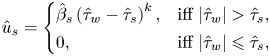 \begin{equation} \hat{u}_{{s}} = \left\{\begin{array}{@{}ll} \hat{\beta}_s \left( \hat{\tau}_{w} - \hat{\tau}_{s} \right)^k, & \text{iff}\ \vert \hat{\tau}_{w} \vert > \hat{\tau}_s, \\ 0, & \text{iff}\ \vert \hat{\tau}_{w} \vert \leqslant \hat{\tau}_s, \end{array} \right. \end{equation}
usually termed as the ‘stick–slip’ law, where  $\hat {u}_{{s}}$ is the slip velocity on the solid surface and $\hat {\tau }_w$ is the shear stress at the solid boundaries. The sliding threshold is called the sliding yield stress – $\hat {\tau }_s$. The slip coefficient and the power index are designated by $\hat {\beta }_s$ and $k$, respectively. Hence, $\hat {\beta }_s$ has the dimension of $m^{2k+1}/N^k.s$ or $m/Pa^k.s$. Its physical interpretation (for the case $k=1$) is the slip length over the local effective viscosity of the fluid, $\hat {\ell }_s / \hat {\mu }_{eff}$. In the entire paper, quantities with a ‘hat’ symbol ( $\hat {\cdot }$) are dimensional and others are dimensionless.
For a deeper understanding of the physical meaning of the slip law (1.1), we consider the simple unidirectional channel Poiseuille flow in the presence of slip of a viscoplastic fluid,
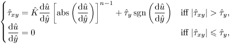 \begin{equation} \left\{\begin{array}{@{}ll} \hat{\tau}_{xy} = \hat{K} \displaystyle \dfrac{\text{d} \hat{u}}{\text{d} \hat{y}} \left[ \text{abs}\left( \dfrac{\text{d} \hat{u}}{\text{d} \hat{y}} \right) \right]^{n-1} + \hat{\tau}_y \,\text{sgn} \left( \dfrac{\text{d} \hat{u}}{\text{d} \hat{y}} \right) & \mbox{iff}\ \vert \hat{\tau}_{xy} \vert > \hat{\tau}_y, \\ \displaystyle \dfrac{\text{d} \hat{u}}{\text{d} \hat{y}} = 0 & \mbox{iff}\ \vert \hat{\tau}_{xy} \vert \leqslant \hat{\tau}_y, \end{array} \right. \end{equation}
where  $\hat {K} (\textrm {Pa} \cdot s^n)$ is the consistency of the fluid and $n$ the power-index (Herschel–Bulkley model), $\hat {u}$ the streamwise velocity, $\hat {\tau }_y$ the material's yield stress, $\hat {\tau }_{xy}$ the shear stress and $\text {sgn}(\cdot )$ and $\text {abs}(\cdot )$ are the sign and absolute value functions. Figure 1 represents the slip law schematically. When the applied pressure gradient is small enough, the wall shear stress ( $\hat {\tau }_w$) lies below the sliding yield stress (figure 1a) and the slip velocity is zero. Since $\hat {\tau }_s$ is always less than the material's yield stress, then there is no flow in the channel. When the pressure gradient is increased beyond $({\rm \Delta} \hat {p}/\hat {L})_c$ where subscript ‘ $_c$’ indicates the critical value, the wall shear stress grows beyond $\hat {\tau }_s$ and the fluid slides over the walls. If the wall shear stress is still less than $\hat {\tau }_y$, then the material moves as a sliding unyielded plug with a constant velocity in the entire gap (see figure 1b). When the pressure gradient is increased, at some point, the wall shear stress exceeds the fluid yield stress and the sheared/yielded regions appear, which at the same time slide over the walls – see figure 1(c). Yet, in the vicinity of the centreline, the shear stress drops below the yield stress and a core unyielded region is formed. The flows corresponding to figures 1(b) and 1(c) are usually termed the fully plugged regime and the deformation regime, respectively.
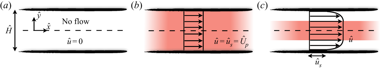
Figure 1. Schematic of the sliding channel flow of a yield-stress fluid; the  $x$-axis is aligned and placed at the axial centreline of the channel which is formed by the two infinite parallel plates separated by the gap $\hat {H}$ and the $y$-axis is in the wall-normal direction: (a) when $\hat {\tau }_w \leqslant \hat {\tau }_s$ there is no flow, (b) when $\hat {\tau }_s < \hat {\tau }_w \leqslant \hat {\tau }_y$ then the fluid in the whole gap slides as an unyielded plug, (c) when $\hat {\tau }_y < \hat {\tau }_w$ then the fluid in the vicinity of the walls ( $\hat {y}_p <\hat {y}$ where $\hat {\tau }_y < \hat {\tau }_{xy}$) yields and at the same time slides over the walls. There is a core unyielded region as well ( $\hat {y} \leqslant \hat {y}_p$).
In the present study, the objective is to systematically address the effect of slip on yield-stress fluid flows and its consequences on the yield limit; not only by conducting numerical simulations, but also by forming a theoretical framework for analysing this type of problem. Although some attempts have been made to solve simple rheometric flows in previous years (Philippou, Kountouriotis & Georgiou Reference Philippou, Kountouriotis and Georgiou2016; Panaseti & Georgiou Reference Panaseti and Georgiou2017; Damianou, Panaseti & Georgiou Reference Damianou, Panaseti and Georgiou2019), still the lack of generic numerical implementation frameworks (especially non-regularized methods) and the absence of adequate theoretical frameworks to attack sliding yield-stress fluid flows are discernible. Hence, in what follows, we aim to partially fill this gap in the literature. Beyond that, we study complex sliding flows such as particle sedimentation and pressure-driven flows in porous media within these frameworks.
The outline of the paper is as follows. In § 2, we set out the slip law beyond 1-D for the yield-stress fluid flows and generalize the numerical algorithm previously proposed for simple 1-D problems. We then benchmark the numerical algorithm for simple channel Poiseuille flow in § 3 and derive some theoretical tools for investigating the sliding flows. This will be followed by addressing the sliding flow about a circular particle and the aspects of the particle yield limit in § 4. The next two sections are devoted to the sliding flows in porous media: in § 5 some general hints are made by studying the flow through model porous media and in § 6 some deeper investigations are carried out by performing numerical simulations in randomized porous media. Finally, some conclusions are drawn in the closing section § 7.
2. Slip law and the numerical algorithm beyond 1-D
In this section, we set out and formulate a sample problem of sliding flow of a yield-stress fluid and generalize the slip law and numerical algorithm for solving such problems beyond 1-D. In what follows, we mainly assume that  $n=1$ (Bingham model). Later in appendix C, we will address how the present framework can be expanded to encompass the other ‘simple’ yield-stress rheological models, e.g. Herschel–Bulkley. However, the majority of the physical discussions (e.g. the yield limit) in the next sections are independent of the value of $n$. We will come back to this point in § 7.
Problem  $\mathbb {P}$. We consider the Stokes flow of a Bingham fluid in $\varOmega \setminus \bar {X}$ (see figure 2) as follows:
 \begin{gather} - \boldsymbol{\nabla} \hat{p} + \boldsymbol{\nabla} \boldsymbol{\cdot} \hat{\boldsymbol{\tau}} + \hat{\rho} \hat{\boldsymbol{f}} = 0, \end{gather}
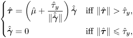 \begin{gather}\left\{\begin{array}{@{}ll} \hat{\boldsymbol{\tau}} = \left( \hat{\mu} + \displaystyle{\dfrac{\hat{\tau}_y}{\Vert \hat{\dot{\boldsymbol{\gamma}}} \Vert}} \right) \hat{\dot{\boldsymbol{\gamma}}} & \mbox{iff}\ \Vert \hat{\boldsymbol{\tau}} \Vert > \hat{\tau}_y, \\ \hat{\dot{\boldsymbol{\gamma}}} = 0 & \mbox{iff}\ \Vert \hat{\boldsymbol{\tau}} \Vert \leqslant \hat{\tau}_y, \end{array} \right. \end{gather}
where  $\hat {p}$ is the pressure, $\hat {\boldsymbol {\tau }}$ the deviatoric stress tensor, $\hat {\rho } \hat {\boldsymbol {f}}$ the body force, $\hat {\rho }$ the fluid density and $\hat {\dot {\boldsymbol {\gamma }}}$ is the rate of deformation tensor. Without loss of generality, we consider no-slip and no-penetration boundary conditions on $\partial \varOmega$ as $\hat {\boldsymbol {u}} = \hat {\boldsymbol {u}}_0$ and the slip boundary condition,
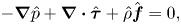
 \begin{equation} \hat{u}_{{s}} = \hat{\boldsymbol{u}}_{{ns}} \boldsymbol{\cdot} \boldsymbol{t} - \boldsymbol{\delta} \hat{\boldsymbol{u}} \boldsymbol{\cdot} \boldsymbol{t} = \left\{ \begin{array}{@{}ll} \hat{\beta}_s \hat{\varLambda} \left( 1 - \displaystyle\dfrac{\hat{\tau}_{s}}{\vert \hat{\varLambda} \vert} \right), & \text{iff}\ \vert \hat{\varLambda} \vert > \hat{\tau}_s, \\ 0, & \text{iff}\ \vert \hat{\varLambda} \vert \leqslant \hat{\tau}_s, \end{array} \right. \end{equation}
on  $\partial X$, where $\hat {u}_{{s}}$ is the slip velocity, $\hat {\boldsymbol {u}}_{{ns}}$ the velocity of the solid boundary $\partial X$ and $\boldsymbol {\delta } \hat {\boldsymbol {u}}$ is the restriction of $\hat {\boldsymbol {u}}$ on $\partial X$: $\hat {\boldsymbol {u}} \to \boldsymbol {\delta } \hat {\boldsymbol {u}}$ as $\hat {\boldsymbol {x}} \to \partial X$. The value of the tangential traction vector (i.e. tangential force per unit area on the solid surface) is shown by $\hat {\varLambda } = [ ( - \hat {p} \boldsymbol {1} + \hat {\boldsymbol {\tau }} ) \boldsymbol {\cdot } \boldsymbol {n} ] \boldsymbol {\cdot } \boldsymbol {t}$, where the normal and tangential unit vectors to the solid surface $\partial X$ are represented by $\boldsymbol {n}$ and $\boldsymbol {t}$, respectively. The no-penetration condition on $\partial X$ reads $\boldsymbol {\delta }\hat {\boldsymbol {u}} \boldsymbol {\cdot } \boldsymbol {n} = \hat {\boldsymbol {u}}_{{ns}} \boldsymbol {\cdot } \boldsymbol {n}$.

Figure 2. Schematic of the problem  $\mathbb {P}$. The full domain is denoted by $\varOmega$, and the solid object on which the flow slides in designated by $X$. The red arrows show the outward unit normal vectors of the solid surface $\partial X$. The boundary of the full domain is $\partial \varOmega$.
Without loss of generality, we fixed  $k$ at unity in the slip law (2.3) and will do so in the rest of the present study. This is supported by experimental observations as well. Seth et al. (Reference Seth, Locatelli-Champagne, Monti, Bonnecaze and Cloitre2012) validated the slip power index of unity for emulsions contacting non-adhering surfaces. Moreover, in separate experimental studies, Poumaere et al. (Reference Poumaere, Moyers-González, Castelain and Burghelea2014) and Daneshi et al. (Reference Daneshi, Pourzahedi, Martinez and Grecov2019) reported $k\approx 1$ for the pressure-driven flows of Carbopol gels with different concentrations and stirring rates during the sample preparation. However, experiments have also revealed that $k \neq 1$ in some cases (Piau Reference Piau2007; Medina-Bañuelos et al. Reference Medina-Bañuelos, Marín-Santibáñez, Pérez-González, Malik and Kalyon2017, Reference Medina-Bañuelos, Marín-Santibáñez, Pérez-González and Kalyon2019). We will discuss these cases in appendix C, as the main objectives/conclusions of the present study are independent of the value of $k$.
$k$.
2.1. Numerical algorithm
The minimization principle for the sliding problem  $\mathbb {P}$ can be derived as
 \begin{align} \mathcal{J}(\hat{\boldsymbol{u}}) & = \frac{\hat{\mu}}{2} \int_{\varOmega \setminus \bar{X}} \hat{\dot{\boldsymbol{\gamma}}} (\hat{\boldsymbol{u}}) \boldsymbol{:} \hat{\dot{\boldsymbol{\gamma}}} (\hat{\boldsymbol{u}}) \,\text{d}\hat{V} + \hat{\tau}_y \int_{\varOmega \setminus \bar{X}} \Vert \hat{\dot{\boldsymbol{\gamma}}} (\hat{\boldsymbol{u}}) \Vert \,\text{d}\hat{V} - \int_{\varOmega \setminus \bar{X}} \hat{\rho} \hat{\boldsymbol{f}} \boldsymbol{\cdot} \hat{\boldsymbol{u}} \,\text{d} \hat{V} \nonumber\\ &\quad + \frac{1}{2 \hat{\beta}_s} \int_{\partial X} \hat{u}_s^2 \,\text{d}\hat{A} + \hat{\tau}_s \int_{\partial X} \vert \hat{u}_s \vert \,\text{d}\hat{A}. \end{align}
For the augmented Lagrangian approach we require to relax the rate of strain tensor to the auxiliary tensor  $\hat {\boldsymbol {q}}$ and the restriction of the velocity vector on $\partial X$ to the auxiliary vector $\hat {\boldsymbol {\xi }}$. Then the saddle-point problem associated with $\mathbb {P}$ is
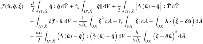 \begin{align} \mathcal{J}(\hat{\boldsymbol{u}},\hat{\boldsymbol{q}},\hat{\boldsymbol{\xi}}) & = \frac{\hat{\mu}}{2} \int_{\varOmega \setminus \bar{X}} \hat{\boldsymbol{q}} \boldsymbol{:} \hat{\boldsymbol{q}}\,\text{d}\hat{V} + \hat{\tau}_y \int_{\varOmega \setminus \bar{X}} \Vert \hat{\boldsymbol{q}} \Vert \,\text{d}\hat{V} + \frac{1}{2} \int_{\varOmega \setminus \bar{X}} \left[ \hat{\dot{\boldsymbol{\gamma}}} \left( \hat{\boldsymbol{u}} \right) - \hat{\boldsymbol{q}} \right] \boldsymbol{:} \hat{\boldsymbol{T}} \,\text{d}\hat{V} \nonumber\\ &\quad - \int_{\varOmega \setminus \bar{X}} \hat{\rho} \hat{\boldsymbol{f}} \boldsymbol{\cdot} \hat{\boldsymbol{u}} ~\text{d} \hat{V} + \frac{1}{2 \hat{\beta}_s} \int_{\partial X} \hat{\boldsymbol{\xi}}^2 \,\text{d}\hat{A} + \hat{\tau}_s \int_{\partial X} \vert \hat{\boldsymbol{\xi}} \vert \,\text{d}\hat{A} + \int_{\partial X} \hat{\boldsymbol{\lambda}} \boldsymbol{\cdot} \left( \hat{\boldsymbol{\xi}} - \boldsymbol{\delta} \hat{\boldsymbol{u}} \right) \text{d}\hat{A} \nonumber\\ & \quad + \frac{a \hat{\mu}}{2} \int_{\varOmega \setminus \bar{X}} \left( \hat{\dot{\boldsymbol{\gamma}}} \left( \hat{\boldsymbol{u}} \right) - \hat{\boldsymbol{q}} \right) \boldsymbol{:} \left( \hat{\dot{\boldsymbol{\gamma}}} \left( \hat{\boldsymbol{u}} \right) - \hat{\boldsymbol{q}} \right) \text{d}\hat{V} + \frac{b}{2 \hat{\beta}_s} \int_{\partial X} \left( \hat{\boldsymbol{\xi}} - \boldsymbol{\delta} \hat{\boldsymbol{u}} \right)^2 \text{d}\hat{A}, \end{align}
where  $a$ and $b$ are arbitrary constants (augmentation parameters); $\hat {\boldsymbol {T}}$ and $\hat {\boldsymbol {\lambda }}$ are the Lagrange multipliers.
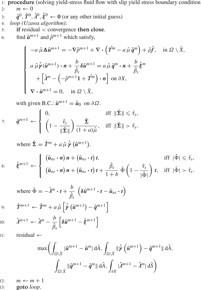
Hence, the Uzawa algorithm in the presence of slip takes the form of algorithm 1. Upon convergence of algorithm 1 with the free augmentation parameters  $a$ and $b$, the Lagrange multiplier $\hat {\boldsymbol {T}}$ converges to the true stress field, $\hat {\boldsymbol {q}}$ to the true rate of strain tensor, Lagrange multiplier $\hat {\boldsymbol {\lambda }}$ to the traction vector on $\partial X$, and auxiliary variable $\hat {\boldsymbol {\xi }}$ to the velocity on $\partial X$.
A mesh adaptation procedure, the same as the one proposed by Roquet & Saramito (Reference Roquet and Saramito2003), could be coupled with the above algorithm to obtain a fine resolution of the yield surfaces. Based on this procedure, the adapted mesh is stretched anisotropically in the direction of the eigenvectors of the Hessian of  $\sqrt {\hat {\mu } \,\hat {\dot {\boldsymbol {\gamma }}} \boldsymbol {:} \hat {\dot {\boldsymbol {\gamma }}} + \hat {\tau }_y \Vert \hat {\dot {\boldsymbol {\gamma }}} \Vert }$, which is the square root of the local energy dissipation. In this study, we implement the entire numerical algorithm in an open-source C $++$ finite element environment – FreeFEM $++$ (Hecht Reference Hecht2012). We have previously validated our numerical implementation and mesh adaptation widely within various studies (Chaparian & Frigaard Reference Chaparian and Frigaard2017b; Chaparian & Tammisola Reference Chaparian and Tammisola2019; Chaparian et al. Reference Chaparian, Izbassarov, De Vita, Brandt and Tammisola2020). Here we will not go into technical details such as the convergence rate, since such details are well-documented in the previous studies – please see, for example, Roquet & Saramito (Reference Roquet and Saramito2008).
In what follows, we quickly validate the algorithm for the sliding flows and most importantly derive variational tools (Mosolov & Miasnikov Reference Mosolov and Miasnikov1965) for a sample problem. These tools will be used to analyse more complex flows in the next sections.
3. Benchmark problem: sliding channel Poiseuille flow
In this section we consider the sliding flow of a Bingham fluid in a channel (Poiseuille flow) – the same as the one shown in figure 1. The walls are denoted by  $\varGamma$ and the full domain by $\varOmega$. We consider two classic formulations: (i) the mobility problem ([M]) where the pressure gradient is applied and the flow rate can be computed and (ii) the resistance problem ([R]) in which flow rate is set and as a result pressure gradient can be computed. We also validate the presented numerical algorithm and derive/revisit some variational tools (Huilgol Reference Huilgol1998) useful for the rest of this study.
3.1. The [M] problem
In this subsection, we use  $\hat {G} \hat {H}^2 /\hat {\mu }$ as the velocity scale, $\hat {G}\hat {H}$ as the characteristic viscous stress to scale the deviatoric stress tensor and $\hat {H} / \hat {\mu }$ to scale the slip coefficient where $\hat {G}$ is the absolute value of the applied pressure-gradient to drive the flow from left to right (in the positive direction of the $x$-axis). Hence, the non-dimensional governing and constitutive equations take the forms
 \begin{equation} \boldsymbol{e}_x + \boldsymbol{\nabla} \boldsymbol{\cdot} \boldsymbol{\tau} = 0 \end{equation}
and
 \begin{equation} \left\{ \begin{array}{@{}ll} \boldsymbol{\tau} = \left( 1 + \displaystyle{\dfrac{Od}{\Vert\dot{\boldsymbol{\gamma}}\Vert}} \right) \dot{\boldsymbol{\gamma}} & \mbox{iff}\ \Vert \boldsymbol{\tau} \Vert > Od, \\ \dot{\boldsymbol{\gamma}} = 0 & \mbox{iff}\ \Vert \boldsymbol{\tau} \Vert \leqslant Od, \end{array} \right. \end{equation}
respectively, and the slip law
 \begin{equation} u_{s} = \left\{ \begin{array}{@{}ll} \beta_s \varLambda \left( 1 - \displaystyle\dfrac{Od_s}{\vert \varLambda \vert} \right), & \text{iff}\ \vert \varLambda \vert > Od_s, \\ 0, & \text{iff}\ \vert \varLambda \vert \leqslant Od_s, \end{array} \right. \end{equation}
where  $Od = {\hat {\tau }_y}/{\hat {H} \hat {G}}$ and $Od_s = {\hat {\tau }_s}/{\hat {H} \hat {G}}$. In what follows, the ratio ${\hat {\tau }_s}/{\hat {\tau }_y}$ is denoted by $\alpha _s$. The analytical solutions to the velocity and stress fields are derived in appendix A.1.
The energy balance equation in the presence of slip is
 \begin{align} & a(\boldsymbol{u},\boldsymbol{u}) + Od \,j(\boldsymbol{u}) + \int_{\varGamma} \vert \sigma_{nt} u_s \vert \,\text{d}S \nonumber\\ &\quad = a(\boldsymbol{u},\boldsymbol{u}) + Od \,j(\boldsymbol{u}) + \frac{1}{\beta_s} \int_{\varGamma} u^2_s \,\text{d}S + Od_s \int_{\varGamma} \vert u_s \vert \,\text{d}S \nonumber\\ & \quad = a(\boldsymbol{u},\boldsymbol{u}) + Od \,j(\boldsymbol{u}) + a_s (u_s,u_s) + Od_s \,j_s(u_s) = \int_{\varOmega} \boldsymbol{u} \boldsymbol{\cdot} \boldsymbol{e}_x \,\text{d}A, \end{align}
where  $a(\boldsymbol {u},\boldsymbol {u}) = \int _{\varOmega } \dot {\boldsymbol {\gamma }} (\boldsymbol {u}) \boldsymbol {:} \dot {\boldsymbol {\gamma }} (\boldsymbol {u}) \,\text {d} A$ and $Od\,j(\boldsymbol {u}) = Od\int _{\varOmega } \Vert \dot {\boldsymbol {\gamma }} (\boldsymbol {u}) \Vert \,\text {d} A$ are the viscous and plastic dissipations, respectively. Please note that the slip dissipation $\int _{\partial X} \vert \sigma _{nt} u_s \vert \,\text {d}S$ can be split into two terms: the ‘viscous’ slip dissipation $(1/\beta _s) \int _{\varGamma } u_s^2\,\text {d}S$ which is designated by $a_s (u_s,u_s)$ in this study and the ‘plastic’ slip dissipation $Od_s \int _{\varGamma } \vert u_s \vert \,\text {d}S$ with $Od_s ~j_s(u_s)$. Moreover, $j(\boldsymbol {u})$ is the normalized plastic dissipation and $j_s(u_s)$ the normalized ‘plastic’ slip dissipation.
We can rearrange the energy balance equation and form a set of inequalities as follows:
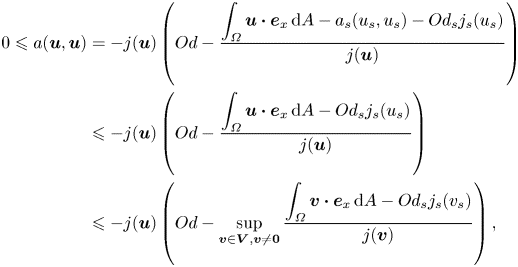 \begin{align} 0 \leqslant a(\boldsymbol{u},\boldsymbol{u}) &= -j(\boldsymbol{u}) \left( Od - \frac{\displaystyle \int_{\varOmega} \boldsymbol{u} \boldsymbol{\cdot} \boldsymbol{e}_x \,\text{d}A - a_s (u_s,u_s) - Od_s j_s (u_s)}{j(\boldsymbol{u})} \right) \nonumber\\ &\leqslant -j(\boldsymbol{u}) \left( Od - \frac{\displaystyle \int_{\varOmega} \boldsymbol{u} \boldsymbol{\cdot} \boldsymbol{e}_x \,\text{d}A - Od_s j_s (u_s)}{j(\boldsymbol{u})} \right) \nonumber\\ &\leqslant -j(\boldsymbol{u}) \left( Od - \sup_{\boldsymbol{v} \in \boldsymbol{V}, \boldsymbol{v} \neq \boldsymbol{0}} \frac{\displaystyle \int_{\varOmega} \boldsymbol{v} \boldsymbol{\cdot} \boldsymbol{e}_x \,\text{d}A - Od_s j_s (v_s)}{j(\boldsymbol{v})} \right), \end{align}
to find the definition of the critical Oldroyd number in the presence of slip as
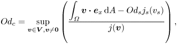 \begin{equation} Od_c = \sup_{\boldsymbol{v} \in \boldsymbol{V}, \boldsymbol{v} \neq \boldsymbol{0}} \left( \frac{\displaystyle \int_{\varOmega} \boldsymbol{v} \boldsymbol{\cdot} \boldsymbol{e}_x \,\text{d}A - Od_s j_s (v_s)}{j(\boldsymbol{v})} \right), \end{equation}
where  $\boldsymbol {v}$ is a velocity test function from the set of all admissible velocity fields $\boldsymbol {V}$. Then it enforces that for $Od_c \leqslant Od$, $a(\boldsymbol {u},\boldsymbol {u})=0$ or $\boldsymbol {u}=0$ (i.e. no flow condition).
We may use (3.6) for calculating  $Od_c$ in simple flows such as Poiseuille flow here: the flow can be postulated by two boundary layers with thickness $\delta$ attached to the walls, through which the slip velocity $U_1$ is connected to the plug velocity $U_2$, then,
 \begin{equation} j(\boldsymbol{v}) \approx 2\frac{U_2 - U_1}{\delta} \delta \ell = 2(U_2 - U_1) \ell\ \&\ j_s (v_s) = 2 U_1 \ell, \end{equation}
where  $\ell$ is the length of the chosen control volume. This suggests,
 \begin{equation} Od_c = \sup_{0 < U_1 \leqslant U_2, (U_1,U_2) \in \mathbb{R}} \frac{U_2 - 2 \,Od_s U_1 }{2 (U_2 - U_1)} = \sup_{0 < U_1 \leqslant U_2, (U_1,U_2) \in \mathbb{R}} \frac{U_2 - 2 \alpha_s Od_c U_1 }{2 (U_2 - U_1)}, \end{equation}
or,
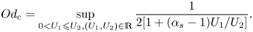 \begin{equation} Od_c = \sup_{0 < U_1 \leqslant U_2, (U_1,U_2) \in \mathbb{R}} \frac{1}{2 [1 + (\alpha_s-1) U_1 / U_2]}. \end{equation}
The maximal value of the argument is  $1/2\alpha _s$ which occurs at $U_1 / U_2 = 1$. Its physical interpretation is that the supremum occurs in the fully sliding regime, which is intuitive. Hence, $Od_c = 1/2\alpha _s$, or in other words, there is no flow if $1/2 \leqslant Od_s$, which is in agreement with the solution of the full equations derived in appendix A.1.
We perform a few simulations for the [M] problem to benchmark the presented algorithm. Figure 3 illustrates different regimes: figure 3(a) compares the computed velocity profile (blue line) in the gap with the analytical solution (red circles) in the fully sliding plug regime ( $Od=1, \alpha _s=0.2\ \&\ \beta _s=0.1$) and figure 3(b) within the deforming regime. Utilizing the mesh adaptation seems more indispensable in the deforming regime compared with the fully sliding plug regime, where velocity gradient is zero. It is clear that the velocity distribution after adaptation (red line) is much closer to the analytical solution (red circles) than the solution of the initial mesh (blue line), and also yields a fine resolution of the yield surfaces – see figure 3(d). We shall mention that the focus of the present study is not on quantifying these improvements by the mesh adaptation, as it has been previously studied in detail (Roquet & Saramito Reference Roquet and Saramito2003, Reference Roquet and Saramito2008; Chaparian & Tammisola Reference Chaparian and Tammisola2019).
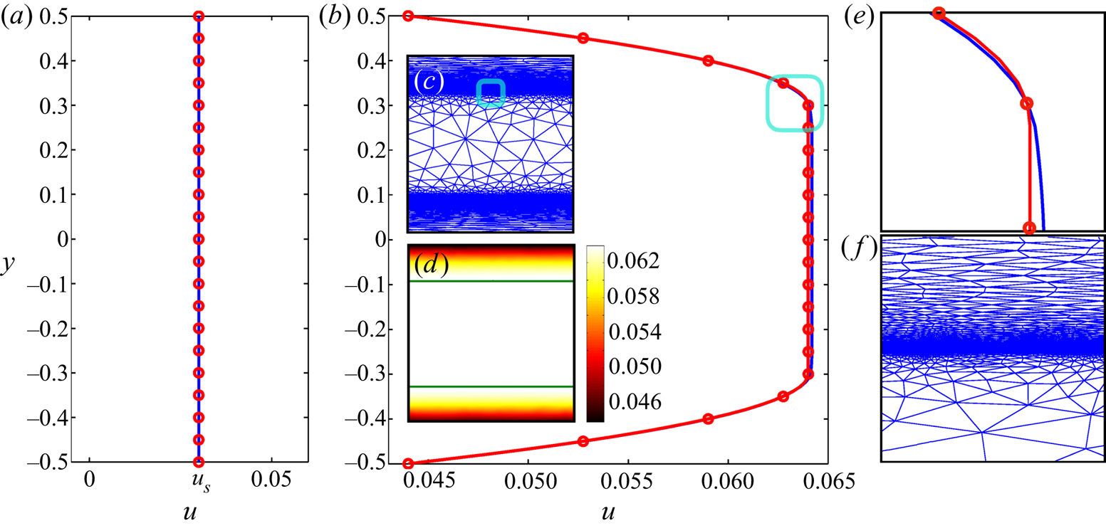
Figure 3. The [M] problem features: (a) velocity profile of the case  $Od=1, \alpha _s=0.2, \beta _s=0.1$ (fully sliding plug); (b) velocity profile of the case $Od=0.3, \alpha _s=0.2, \beta _s=0.1$ (deforming regime); (c) the mesh after five cycles of adaptation associated with panel (b); (d) velocity contour associated with panel (b), the green lines show the yield surfaces; (e,f) close-up of the cyan windows in the panels (b,c), respectively. Please note that in panels (a,b,e) the blue line shows the numerical data corresponding to the initial mesh, the red line corresponds to the adapted mesh (the mesh shown in the panel (c)) and the red circles are the analytical solution; see appendix A.1.
3.2. The [R] problem
Here, we reformulate the problem in the resistance scalings and the quantities are designated with asterisk sign ( $*$) to prevent any potential confusion with the [M] problem. In the resistance formulation, the velocity is scaled with the mean bulk velocity, $\hat {U}=\hat {Q}/\hat {H}$, and as a result, there is always a non-zero flow with the flow rate equal to unity ( $Q^*=1$), whether the flow is in the deforming regime or the fully sliding plug regime. The deviatoric stress and pressure are scaled with the characteristic viscous stress, $\hat {\mu } \hat {U}/\hat {H}$, hence,
 \begin{equation} G^* \boldsymbol{e}_x + \boldsymbol{\nabla} \boldsymbol{\cdot} \boldsymbol{\tau}^* = 0 \end{equation}
and
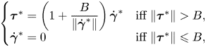 \begin{equation} \left\{ \begin{array}{@{}ll} \boldsymbol{\tau}^* = \left( 1 + \displaystyle{\dfrac{B}{\Vert\dot{\boldsymbol{\gamma}}^*\Vert}} \right) \dot{\boldsymbol{\gamma}}^* & \mbox{iff}\ \Vert \boldsymbol{\tau}^* \Vert > B, \\ \dot{\boldsymbol{\gamma}}^* = 0 & \mbox{iff}\ \Vert \boldsymbol{\tau}^* \Vert \leqslant B, \end{array} \right. \end{equation}
with the boundary condition,
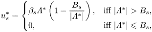 \begin{equation} u^*_{{s}} = \left\{\begin{array}{@{}ll} \beta_s \varLambda^* \left( 1 - \displaystyle\dfrac{B_{s}}{\vert \varLambda^* \vert} \right), & \text{iff}\ \vert \varLambda^* \vert > B_{s}, \\ 0, & \text{iff}\ \vert \varLambda^* \vert \leqslant B_{s}, \end{array} \right. \end{equation}
on the walls govern the [R] problem. Please note that  $G^*$ is the absolute value of the pressure gradient which enforces the unity flow rate for a given Bingham number $( {\hat {\tau }_y \hat {H}}/{\hat {\mu } \hat {U}} )$, $\alpha _s$ and $\beta _s$. The energy balance equation in this case is
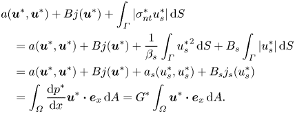 \begin{align} & a(\boldsymbol{u}^*,\boldsymbol{u}^*) + B j(\boldsymbol{u}^*) + \int_{\varGamma} \vert \sigma^*_{nt} u^*_s \vert \, \text{d}S \nonumber\\ &\quad = a(\boldsymbol{u}^*,\boldsymbol{u}^*) + B j(\boldsymbol{u}^*) + \frac{1}{\beta_s} \int_{\varGamma} {u^*_s}^2 \,\text{d}S + B_s \int_{\varGamma} \vert u^*_s \vert \,\text{d}S \nonumber\\ & \quad = a(\boldsymbol{u}^*,\boldsymbol{u}^*) + B j(\boldsymbol{u}^*) + a_s (u^*_s,u^*_s) + B_s j_s (u^*_s) \nonumber\\ &\quad = \int_{\varOmega} \frac{\text{d} p^*}{\text{d} x} \boldsymbol{u}^* \boldsymbol{\cdot} \boldsymbol{e}_x \,\text{d}A = G^* \int_{\varOmega} \boldsymbol{u}^* \boldsymbol{\cdot} \boldsymbol{e}_x \,\text{d}A. \end{align}
 Frigaard (Reference Frigaard2019) has shown that at the yield limit ( $B \to \infty$), viscous dissipation is at least one order of magnitude less than the plastic dissipation (when $B \to \infty$: $a(\boldsymbol {u}^*,\boldsymbol {u}^*) \ll B j(\boldsymbol {u}^*)$). With a little extra effort, we can show that this applies to $a_s (u^*_s,u^*_s)$ and $B_s j_s (u^*_s)$ as well, knowing that $u_s^* \leqslant 1$ (from the continuity equation $Q^*=1$) and $B_s \to \infty$ in this limit. Exploiting that generally the mapping between [M] and [R] problems is attainable via $Q = {Od}/{B}$ or $G^* = {B}/{Od}$, one can extract the critical Oldroyd number from the [R] formulation through
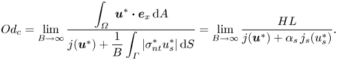 \begin{equation} Od_c = \lim_{B \to \infty} \frac{\displaystyle \int_{\varOmega} ~ \boldsymbol{u}^* \boldsymbol{\cdot} \boldsymbol{e}_x \,\text{d}A}{j(\boldsymbol{u}^*)+\displaystyle \frac{1}{B} \int_{\varGamma} \vert \sigma^*_{nt} u^*_s \vert \,\text{d}S} = \displaystyle \lim_{B \to \infty} \frac{HL}{j(\boldsymbol{u}^*)+\alpha_s \,j_s (u^*_s)}. \end{equation}
 To explain the relation between [R] and [M] problems further, we consider some examples in figure 4. The analytical solutions to (3.10)–(3.12) of the [R] problem are derived in appendix A.2. The absolute value of the pressure gradient versus the Bingham number under the no-slip condition and the sliding flow  $\alpha _s=0.2\ \&\ \beta _s=0.1$ are shown with the continuous black and red lines, respectively. While for both type of flows an increase in $G^*$ by increasing Bingham number can be observed, they display different trends. This can be explained by knowing that beyond a critical Bingham number ( $\bar {B} = 1/\beta _s (1-\alpha _s) \leqslant B$), the sliding flow state switches from the deforming regime to the fully sliding plug regime. Only at large enough Bingham numbers ( $B \to \infty$), we can use the numerical data to extract the yield limit. This is illustrated in figure 4 by the dotted lines, where at $B \to \infty$, $G^*$ asymptotes to $2B$ and $2 \alpha _s B = 0.4 B$ for no-slip and the sample sliding flow considered, respectively. In this limit, $j(\boldsymbol {u}^*)$ (dashed lines in figure 4) asymptotes to 2 and 0 for the no-slip and sliding flows: this is equivalent to $Od_c = 1/2$ and $1/2 \alpha_s$, respectively, knowing that $j_s (u_s)$ asymptotes to 2 for the sliding flows at sufficiently large Bingham numbers (follow the red dashed-dotted line in figure 4). These results are the same as the ones derived in appendix A.1 considering the [M] formulation. Please note that due to the log–log scaling used in figure 4, $j(\boldsymbol {u}^*)$ corresponds to the sliding flow, which is exactly equal to zero for $\bar {B} \leqslant B$ is not visible; however, its fast decay is clear: $j(\boldsymbol {u}^*)$ is almost equal to $10^{-2}$ for $B\approx 11.85$ where $\bar {B}(\alpha _s=0.2\ \&\ \beta _s=0.1) = 12.5$. From a different perspective, the inset in figure 4 shows how mesh adaptation helps us to achieve more accurate results.
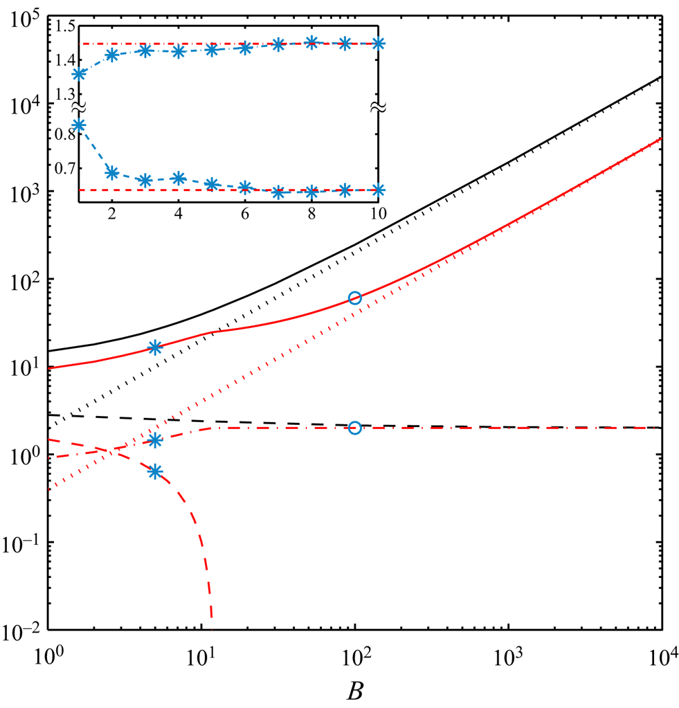
Figure 4. Features of the [R] problem for no-slip (in black) and sliding flow  $\alpha _s=0.2\ \&\ \beta _s = 0.1$ (in red). Lines represent analytically calculated values (see appendix A.2): continuous lines, $G^*$; dashed lines, $j(\boldsymbol {u}^*)$; dashed-dotted line, $j_s (u_s)$. The black dotted line is the asymptotic scaling $2 B$ and red dotted line $2 \alpha _s B = 0.4 B$. The asterisk symbols mark the computational data in the deforming regime and circle symbols in the fully sliding regime. Inset ( $B=5, B_s = 1\ \&\ \beta _s =0.1$): $j(\boldsymbol {u}^*)$ (cyan dashed line and asterisks) and $j_s (u_s)$ (cyan dashed-dotted line and asterisks) versus the cycles of mesh adaptation index with red lines showing the analytically calculated values in appendix A.2.
4. Slippery particle motion
Particle motion in yield-stress fluids has been considered in numerous studies ranging from numerical simulations (Beris et al. Reference Beris, Tsamopoulos, Armstrong and Brown1985; Tokpavi, Magnin & Jay Reference Tokpavi, Magnin and Jay2008; Putz & Frigaard Reference Putz and Frigaard2010; Nirmalkar, Chhabra & Poole Reference Nirmalkar, Chhabra and Poole2012; Fraggedakis, Dimakopoulos & Tsamopoulos Reference Fraggedakis, Dimakopoulos and Tsamopoulos2016; Chaparian & Frigaard Reference Chaparian and Frigaard2017a,Reference Chaparian and Frigaardb; Izbassarov et al. Reference Izbassarov, Rosti, Ardekani, Sarabian, Hormozi, Brandt and Tammisola2018) to experimental validations/extensions (Jossic & Magnin Reference Jossic and Magnin2001; Putz et al. Reference Putz, Burghelea, Frigaard and Martinez2008; Tokpavi et al. Reference Tokpavi, Jay, Magnin and Jossic2009). Unfortunately, fewer studies are devoted to investigating the effect of slip on the flow field around the particle surface. Although Fraggedakis et al. (Reference Fraggedakis, Dimakopoulos and Tsamopoulos2016) used the Navier-slip law in their simulations, the emphasis of their study was on the effect of elasticity of the yield-stress fluid in the particle sedimentation problem. On the experimental side, Jossic & Magnin (Reference Jossic and Magnin2001) reported the drag coefficient of the particle moving in a Carbopol gel and showed that for particles with smooth surfaces, the drag coefficient is smaller compared with the rough particles that prevent slip which is intuitive. However, the mentioned authors did not quantify the slip velocity/law on the particle surface and rather qualitatively addressed the effect of slip. In this section, we will shed light on the effect of slippery motion of the yield-stress fluid about a circular two-dimensional (2-D) particle and in detail will address the yield limit under this condition.
Flow configuration: the horizontal symmetry axis of the particle is aligned with the  $x$-axis (positive direction to the right) and the vertical one by $y$-axis (positive direction upward) where the origin of the coordinate system is fixed at the particle centre. The fluid flow about the particle ( $X$) with its radius $\hat {R}$ as the length scale can be described again by two formulations.
(i) The [R] formulation, where the particle is dragged through the fluid with a prescribed velocity $\hat {V}_p^*$ as the boundary condition. Hence, the drag force $\hat {F}^*_D$ can be calculated. In this formulation, $\hat {V}_p^*$ is used as the velocity scale and $\hat {\mu } \hat {V}_p^* / \hat {R}$ as the characteristic viscous stress to scale the deviatoric stress tensor and the pressure, hence the governing equation is
(4.1)with (3.11) and (3.12) as the constitutive and the slip law, respectively, where\begin{equation} {-}\boldsymbol{\nabla}p^* + \boldsymbol{\nabla} \boldsymbol{\cdot} \boldsymbol{\tau}^*=0\quad \text{in}\ \varOmega \setminus \bar{X}\ \&\ \boldsymbol{u}_{ns}^*=-\boldsymbol{e}_y\quad \text{on}\ \partial X \end{equation}$B=\hat {\tau }_y \hat {R}/ \hat {\mu } \hat {V}^*_p$. The drag force on the particle can be computed as a result from
(4.2)\begin{equation} a(\boldsymbol{u}^*,\boldsymbol{u}^*) + B j(\boldsymbol{u}^*) + a_s (u^*_s,u^*_s) + B_s j_s (u^*_s) = \int_{\partial X} \left( \boldsymbol{\sigma}^* \boldsymbol{\cdot} \boldsymbol{n} \right) \boldsymbol{\cdot} \boldsymbol{e}_y \,\text{d}S = F^*_D. \end{equation}
$\hat {V}_p^*$ as the boundary condition. Hence, the drag force $\hat {F}^*_D$ can be calculated. In this formulation, $\hat {V}_p^*$ is used as the velocity scale and $\hat {\mu } \hat {V}_p^* / \hat {R}$ as the characteristic viscous stress to scale the deviatoric stress tensor and the pressure, hence the governing equation is
(4.1)with (3.11) and (3.12) as the constitutive and the slip law, respectively, where\begin{equation} {-}\boldsymbol{\nabla}p^* + \boldsymbol{\nabla} \boldsymbol{\cdot} \boldsymbol{\tau}^*=0\quad \text{in}\ \varOmega \setminus \bar{X}\ \&\ \boldsymbol{u}_{ns}^*=-\boldsymbol{e}_y\quad \text{on}\ \partial X \end{equation}$B=\hat {\tau }_y \hat {R}/ \hat {\mu } \hat {V}^*_p$. The drag force on the particle can be computed as a result from
(4.2)\begin{equation} a(\boldsymbol{u}^*,\boldsymbol{u}^*) + B j(\boldsymbol{u}^*) + a_s (u^*_s,u^*_s) + B_s j_s (u^*_s) = \int_{\partial X} \left( \boldsymbol{\sigma}^* \boldsymbol{\cdot} \boldsymbol{n} \right) \boldsymbol{\cdot} \boldsymbol{e}_y \,\text{d}S = F^*_D. \end{equation}(ii) The [M] formulation, where the buoyancy of the particle is known and it falls freely under the action of the gravity
$-\hat {g} \boldsymbol {e}_y$. Hence, the settling velocity of the particle $\hat {V}_p$ can be calculated as a result. In this formulation, velocity is scaled with ${\rm \Delta} \hat {\rho } \hat {g} \hat {R}^2 / \hat {\mu }$: the velocity scale obtained via balancing the buoyancy stress with the characteristic viscous stress. Please note that here $\hat {g}$ is the gravitational acceleration and ${\rm \Delta} \hat {\rho }$ is the density difference between the particle and the suspending fluid. Hence, the governing equation is
(4.3)where\begin{equation} {-}\boldsymbol{\nabla}p + \boldsymbol{\nabla} \boldsymbol{\cdot} \boldsymbol{\tau} - \frac{\rho}{1-\rho} \boldsymbol{e}_y =0\quad \text{in} \ \varOmega \setminus \bar{X}\ \text{and} \int_{\partial X} \left( \boldsymbol{\sigma} \boldsymbol{\cdot} \boldsymbol{n} \right) \boldsymbol{\cdot} \boldsymbol{e}_y \,\text{d}S=\frac{\rm \pi}{1-\rho} \end{equation}$\rho$ is the ratio of the fluid density to the particle one (i.e. $\hat {\rho }_f / \hat {\rho }_p$). The constitutive and slip laws are the same as (3.2) and (3.3), respectively, with a slight difference: the yield number $Y$ is substituted for the Oldroyd number in the particle sedimentation problem; indeed, $Y=\hat {\tau }_y / {\rm \Delta} \hat {\rho } \hat {g} \hat {R}$.


The yield limit can be well understood using either the [R] or [M] formulations knowing the mapping between these two formulations:  $Y = {\rm \pi}B / F^*_D$ or $B=Y/V_p$. In the [R] formulation, the particle never stops because the particle velocity is set as the boundary condition, yet, in the yield limit $B \to \infty$, the drag force also goes to infinity. However, in the [M] problem, for a large enough yield number $(Y > Y_c)$, the yield stress can overcome the buoyancy of the particle and makes it stationary suspended. The connection between these two situations can be well discussed by the ‘plastic drag coefficient’,
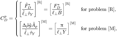 \begin{equation} C_D^p = \left\{ \begin{array}{@{}ll} \left[ \dfrac{\hat{F}^*_D}{\hat{\ell}_\bot \hat{\tau}_Y} \right]^{[\textrm{R}]} = \left[ \dfrac{F^*_D}{\ell_\bot B} \right]^{[\textrm{R}]} & \mbox{for problem [R]}, \\ \left[ \dfrac{ {\rm \Delta}\hat{\rho} \hat{g} \hat{A}_p}{\hat{\ell}_\bot \hat{\tau}_Y} \right]^{[\textrm{M}]} = \left[ \dfrac{\rm \pi}{\ell_\bot Y} \right]^{[\textrm{M}]} & \mbox{for problem [M]}, \end{array} \right. \end{equation}
where  $\ell _\bot$ is the width of the particle perpendicular to the flow direction ( $\ell _\bot =2$) and $\hat {A}_p$ is the area of the 2-D particle (i.e. ${\rm \pi} \hat {R}^2$ here). Then, the critical plastic drag coefficient (i.e. plastic drag coefficient at the yield limit) can be converted easily to the critical yield number,
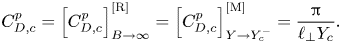 \begin{equation} C_{D,c}^p = \left[ C_{D,c}^p \right]^{[\textrm{R}]}_{B \to \infty} = \left[ C_{D,c}^p \right]^{[\textrm{M}]}_{Y \to Y_c^-} = \frac{\rm \pi}{\ell_\bot Y_c}. \end{equation}
For more details please see Chaparian & Frigaard (Reference Chaparian and Frigaard2017b). For instance, for a 2-D circle, as has been extensively validated (Tokpavi et al. Reference Tokpavi, Magnin and Jay2008; Putz & Frigaard Reference Putz and Frigaard2010; Chaparian & Frigaard Reference Chaparian and Frigaard2017a,Reference Chaparian and Frigaardb), the critical plastic drag coefficient under the no-slip condition is 11.94, which yields to  $Y_c=0.1316$.
Regarding the computational details, we conduct the same strategy as in our previous studies (Chaparian & Frigaard Reference Chaparian and Frigaard2017a,Reference Chaparian and Frigaardb; Iglesias et al. Reference Iglesias, Mercier, Chaparian and Frigaard2020). The computational box ( $\varOmega$) is chosen large enough to ensure independency from far-field conditions (Chaparian, Wachs & Frigaard Reference Chaparian, Wachs and Frigaard2018). The boundary condition $\boldsymbol {u}^*=0$ is enforced on $\partial \varOmega$.
The yield limit of particle motion in a quiescent yield-stress fluid is directly relevant to the lateral resistance of an object (e.g. a pile) in a perfectly plastic medium (e.g. soil) which can be investigated by method of characteristics (i.e. slipline solution) due to the hyperbolic nature of the equations. We briefly revisit this problem in the next subsection.
4.1. Revisiting the slipline solution and lower- and upper-bound calculations
In a deformed perfectly plastic medium, the second invariant of the stress is equal to  $B$ everywhere. The equilibrium equations for the unrestricted 2-D plastic flow then form a closed set of hyperbolic equations for which there are two families of orthogonal characteristic lines: the $\alpha$- and $\beta$-families (Hill Reference Hill1950; Chakrabarty Reference Chakrabarty2012). Physically, these lines (termed as sliplines) show the direction of the maximum shear stress which is equal to $B$. Properties of these lines facilitate studying the ‘yield limit’ in various viscoplastic problems (Dubash et al. Reference Dubash, Balmforth, Slim and Cochard2009; Chaparian & Frigaard Reference Chaparian and Frigaard2017a,Reference Chaparian and Frigaardb; Chaparian & Nasouri Reference Chaparian and Nasouri2018; Hewitt & Balmforth Reference Hewitt and Balmforth2018). However, finding the sliplines itself is not trivial in some complex problems. Indeed, the sliplines assist us in postulating admissible stress and velocity fields which yield to finding the lower and upper bounds, respectively, of the load limit.
Initially investigated by Randolph & Houlsby (Reference Randolph and Houlsby1984), a slipline solution was devised for calculating the lateral resistance of a circular pile in soil (considered as a perfectly plastic material), taking into account the effect of soil adhesion at the pile–soil interface,  $\widetilde {\alpha _s}$. In other words, the tangential shear stress at the pile-soil interface is assumed to be equal to $\tilde {\alpha }_s B$. Although widely believed that the Randolph & Houlsby (Reference Randolph and Houlsby1984) solution is exact (lower and upper bounds of the load/drag are the same for the whole range of $\tilde {\alpha }_s$), an issue was firstly detected by Murff, Wagner & Randolph (Reference Murff, Wagner and Randolph1989): for $\tilde {\alpha }_s < 1$, there is a region in the vicinity of the pile surfaces in which the rate of strain is negative and its absolute value should be taken into account in calculating the upper bound to avoid negative plastic dissipation. If one does so, then there is a discrepancy between the lower and upper bounds. Later, Martin & Randolph (Reference Martin and Randolph2006) proposed two new postulated velocity fields which improved the upper-bound predictions to some extent; one for small ( $\tilde {\alpha }_s \to 0$) and the other one for large ( $\tilde {\alpha }_s \to 1$) soil adhesion factors. By combining these two mechanisms, Martin & Randolph (Reference Martin and Randolph2006) proposed an alternative mechanism which markedly shrinks the uncertainty between the lower and upper bounds predictions for the entire range of $\tilde {\alpha }_s$. We will quickly review the lower- (Randolph & Houlsby Reference Randolph and Houlsby1984) and upper-bound (Martin & Randolph Reference Martin and Randolph2006) solutions here; however, for more details, readers are referred to the original references.
The first family of sliplines in this problem are straight lines that make a  ${{\rm \pi} }/{4}-{\psi }/{2}$ angle with the pile surface (say $\alpha$-lines) where $\psi =\sin ^{-1} \tilde {\alpha }_s$. Figure 5 represents these lines in cyan colour. The initial $\alpha$-line is $AB$ which makes a ${\rm \pi} /4$ angle with the vertical symmetry line since $\tilde {\tau }_{xy}$ is zero on $OB$. Hence, the region enclosed between $AB$ and the pile surface is the plug region shown in light grey. The $\alpha$-lines from $AB$ to $CD$ can be found easily as discussed above; the corresponding $\beta$-lines are curved lines which are the involutes unwrapped from an imaginary concentric circle – the evolute – with radius $\eta =\cos (\frac {1}{2} \cos ^{-1} \tilde {\alpha }_s )$ shown with a dashed white line. Please note that indeed $\alpha$-lines can be introduced as tangents of this imaginary circle as well. From $CD$ to $CE$,
$CE$,  $\alpha$-lines are spokes of a fan centred at $C$; hence, the $\beta$-lines in this part are arcs of concentric circles at point $C$.
$C$.
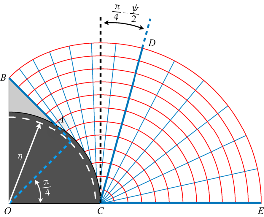
Figure 5. Schematic of the sliplines about a 2-D circle. The  $\alpha$-lines are in cyan colour and $\beta$-lines in red. Only a quarter of the whole domain is shown due to symmetry.
Hencky's equations (Hill Reference Hill1950),
 \begin{equation} \tilde{p}+2B\theta=\textrm{const}.\ \text{along an $\alpha$-line and}\ \tilde{p}-2B\theta=\textrm{const}.\ \text{along a $\beta$-line,} \end{equation}
provide the tool for finding the admissible stress field associated with these sliplines which can be used for calculating the lower bound of the plastic drag coefficient. Here,  $\theta$ is the anticlockwise orientation of the $\alpha$-lines made with the $x$-axis (aligned with $OE$). The individual stress contributions can be written as
 \begin{equation} \tilde{\sigma}_x = -\tilde{p}-B \sin (2\theta),\quad \tilde{\sigma}_y = -\tilde{p}+B \sin (2\theta),\quad \tilde{\tau}_{xy} = B \cos (2\theta) \end{equation}
in the new curvilinear coordinates  $\alpha$ and $\beta$. Then the lower bound can be calculated as
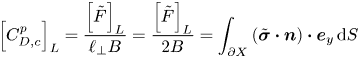 \begin{equation} \left[ C_{D,c}^p \right]_L = \frac{\left[ \tilde{F} \right]_L}{\ell_{\bot} B} = \frac{\left[ \tilde{F} \right]_L}{2B} = \int_{\partial X} \left( \tilde{\boldsymbol{\sigma}} \boldsymbol{\cdot} \boldsymbol{n} \right) \boldsymbol{\cdot} \boldsymbol{e}_y \,\text{d}S \end{equation}
which basically consists of four individual contributions in the shown quadrant: shear force acting on  $AB$,
$AB$,  $B \sin (\psi /2)$; shear force acting on $AC$,
$AC$,  $B \sin \psi \cos (\psi /2)$; normal force acting on $AB$,
$AB$,  $B ( c + {3{\rm \pi} }/{2} ) \sin ({\psi }/{2})$; and normal force acting on $AC$,
$AC$,
 \begin{align} B \left\{ c \left[ 1 - \sin\left(\frac{\psi}{2}\right)\right] + \left[ 2 \cos\left(\frac{\psi}{2}\right) + \frac{\rm \pi}{2} + \psi + \cos\psi - \left( \frac{3{\rm \pi}}{2} + \cos\psi\right) \sin\left(\frac{\psi}{2}\right)\right]\right\}, \end{align}
where  $cB$ is the reference mean stress, $( \tilde {\sigma }_x + \tilde {\sigma }_y )/2$, on $CE$ (position of the centre of the Mohr circle). Please note that $c$ will be eliminated if all four quadrants are taken into account. Hence, the total lower bound of the plastic drag coefficient will be
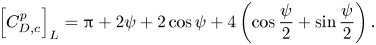 \begin{equation} \left[ C_{D,c}^p \right]_L = {\rm \pi}+ 2 \psi + 2 \cos \psi + 4 \left( \cos \frac{\psi}{2} + \sin \frac{\psi}{2} \right). \end{equation}
The upper-bound calculation can be performed by postulating admissible velocity fields. Geiringer equations (Hill Reference Hill1950) make it feasible via slipline solution,
 \begin{equation} \text{d}\tilde{u}_{\alpha} - \tilde{u}_{\beta} \,\text{d}\theta=0\ \text{along an $\alpha$-line}\ \&\ \text{d}\tilde{u}_{\beta} + \tilde{u}_{\alpha} \,\text{d}\theta=0 \ \text{along a $\beta$-line}, \end{equation}
where  $\tilde {u}_{\alpha }$ and $\tilde {u}_{\beta }$ are the velocities in the directions $\alpha$ and $\beta$ in the new curvilinear coordinate system. Based on these equations, Randolph & Houlsby (Reference Randolph and Houlsby1984) proposed a mechanism (see figure 6a) in which velocity along $\alpha$-lines is zero and along each $\beta$-line is a constant, which can be found by considering a no-penetration condition on the pile or fore-and-aft plugs surface. As mentioned above, this mechanism leads to a relatively large uncertainty with the lower-bound solution for $\tilde {\alpha }_s \neq 1$. Martin & Randolph (Reference Martin and Randolph2006) improved this mechanism by substituting a rotating rigid block (blue region in figure 6b) in the middle of the domain with angular velocity $\omega$ compatible with the no-penetration boundary condition on the pile surface; the centre of that is determined by the angle $\gamma$ and the imaginary evolute circle of radius $\eta$. By optimizing for $\gamma$, one can markedly reduce the uncertainty between the lower and upper bounds of $C_{D,c}^P$.

Figure 6. Schematic of the upper-bound mechanisms: (a) associated with the sliplines (Randolph & Houlsby Reference Randolph and Houlsby1984), (b) combined mechanism (Martin & Randolph Reference Martin and Randolph2006) with the blue region rotating as an unyielded block. Black arrows show velocity vectors. For a better representation, in this schematic the pile velocity is assumed to be  $\boldsymbol {e}_y$. Nevertheless, it should be noted that the flow has fore-and-aft symmetry.
It is worth mentioning that although  $\tilde {\alpha }_s$ and $\alpha _s$ do not have exactly the same physical origins, in what follows, we show that both display the same effect in the current problem and can be used interchangeably. Nevertheless, we should note that, $\alpha _s B$ in the viscoplastic fluid mechanics context not only marks the boundary between the presence of sliding or no-slip flow on the solid surface, but actually also controls the yield limit (see figure 1): for instance in the case of $\alpha _s =1$, the limit of flow/no-flow reduces to having stress as large as $B$ on the solid surfaces. Without a doubt, when there is a flow, it slides over solid boundaries depending on $\beta _s$ in this case. Yet, the case of $\alpha _s=1$ shares the same yield limit characteristics with the no-slip condition. In the perfectly plastic mechanics context, $\tilde {\alpha }_s B$ roughly has the same interpretation since if the tangential shear stress on the solid boundary is less than that, then there are no deformed regions. Indeed, this is the strict condition at the yield limit in a deformed perfectly plastic solid.
4.2. Results
Figure 7(a) represents the plastic drag coefficient versus the Bingham number under different conditions. As shown by Putz & Frigaard (Reference Putz and Frigaard2010) and Chaparian & Frigaard (Reference Chaparian and Frigaard2017b), with the no-slip condition on a circular particle surface,  $\lim _{B \to \infty }C_D^p = C_{D,c}^p \approx 11.94$ which is the value that can be obtained from the expression (4.10) as well when $\tilde {\alpha }_s=1$. Three main points can be drawn from figure 7(a) as follows.
(i) Plastic drag coefficients associated with the sliding flows over the particle surface are smaller compared with the same Bingham number flows with the no-slip condition. This seems intuitive and as mentioned has been validated experimentally by Jossic & Magnin (Reference Jossic and Magnin2001).
(ii) The plastic drag coefficient decreases by increasing Bingham number and reaches a plateau when
$B \to \infty$. More interestingly, the critical plastic drag coefficient associated with the flows of the same $\alpha _s$ asymptote to a same limiting value (see asterisks and circles). Indeed, $C_{D,c}^p$ is only a function of $\alpha _s$. However, in the Newtonian limit, $B \to 0$, this is $\beta _s$ which controls $C_D^p$ (see stars and circles).(iii) The lower-bound estimations from the slipline solutions accurately predicts
$C_{D,c}^p$.


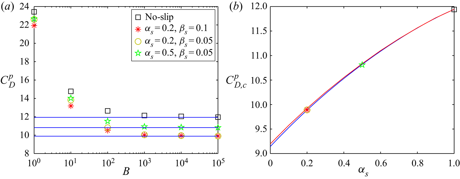
Figure 7. (a) Plastic drag coefficient versus the Bingham number for different  $\alpha _s$ and $\beta _s$. The continuous blue lines are lower-bound estimations for $\tilde {\alpha }_s = 0.2$, 0.5 and 1. (b) Critical plastic drag coefficient versus $\alpha _s$. The blue line is the lower-bound estimation and the red line shows the upper-bound estimation by the combined mechanism (Martin & Randolph Reference Martin and Randolph2006) with the same symbol interpretation as panel (a).
Figure 7(b) compares the lower and upper bounds of the critical plastic drag coefficient with the data obtained by the numerical computations. It clearly shows that even within the sliding flow context, perfectly plastic theories could be useful in investigating the yield limit. It is worth mentioning that, as investigated by Chaparian & Frigaard (Reference Chaparian and Frigaard2017b) in detail, although the computations and slipline analysis display same behaviours to some extent for the no-slip case, the envelope of the characteristics does not agree fully with the yield surfaces in the viscoplastic computations. Both the characteristics solution and the viscoplastic computation predict rigid caps fore-and-aft of the particle (although they are not exactly the same size), whereas the viscoplastic solution also has kidney plug regions along the side of the cylinder. The velocity fields are not exactly equal either – see figure 4 of the mentioned reference. The perfectly plastic velocity has discontinuities which are diffused in the viscoplastic field by the narrow viscous boundary layers. Given the discrepancies in both stress and velocity fields for the no-slip case, it is perhaps interesting that slipline solutions still predict the yield limit very well. Figure 8 reveals that these differences exist in the sliding flows as well. Figure 8(a) sketches the sliplines for the case  $\tilde {\alpha }_s=0.2$, and figure 8(c) shows the computed contours of velocity for the case $\alpha _s=0.2~\&~\beta _s=0.1$ at $B=10^5$. Figures 8(b) and 8(d) make the comparison possible with the no-slip condition. The frontal caps are significantly smaller for $\alpha _s=0.2$ while the side
kidneys are bigger and are in touch with the particle surface.
$\alpha _s=0.2$ while the side
kidneys are bigger and are in touch with the particle surface.
Figure 8. Sliplines for the case (a)  $\tilde {\alpha }_s=0.2$ and (b) no-slip ( $\tilde {\alpha }_s=1$); $\alpha$-lines in blue and $\beta$-lines in red while the rigid caps stock to the particle surface represented in light grey. The other panels show the contour of $\vert \boldsymbol {u}^* \vert$ at $B=10^5$: (c) $\alpha _s=0.2\ and\ \beta _s=0.1$; and (d) no-slip flow. Green lines in panels (c,d) represent the yield surfaces.
Figure 9 closely monitors these differences for the case  $\alpha _s=0.5$. Figure 9(a) shows the contour of velocity in the viscoplastic problem with yield surfaces in continuous green, whereas ‘yield surfaces’ predicted by the combined upper-bound mechanism (Martin & Randolph Reference Martin and Randolph2006) are shown with discontinuous blue lines. Moreover, figure 9(c) compares velocity distributions along the horizontal symmetry line: the two red lines represent the ones associated with the upper-bound mechanisms by Martin & Randolph (Reference Martin and Randolph2006) (continuous) and Randolph & Houlsby (Reference Randolph and Houlsby1984) (discontinuous), while the computed velocities for different Bingham numbers are shown in blue colours; the darker it is the higher the Bingham number. As $B$ increases, the velocity distributions get closer to the ones predicted by the upper-bound mechanisms, especially the combined mechanism where even the slip velocity on the particle surface at the equator is predicted correctly. Nevertheless, again the discontinuities in the perfectly plastic solution are replaced by the viscous boundary layers in the viscoplastic solutions.

Figure 9. Features of the flow about a particle  $\alpha _s=0.5\ \&\ \beta _s=0.05$: (a) velocity contour ( $\vert \boldsymbol {u}^* \vert$) at $B=10^5$, the green lines show the yield surfaces and blue discontinuous lines are yield surfaces predicted in combined upper-bound mechanism (Martin & Randolph Reference Martin and Randolph2006) with $\eta =0.866 \text{ and } \gamma =20.8^\circ$ and cyan discontinuous lines mark the start and end spokes of the rigid zones; (b) contour of $\log _{10} (\Vert \dot {\boldsymbol {\gamma }}^* \Vert )$; (c) velocity profile comparison in simulations with increasing Bingham number ( $B=10$, 100 and $10^5$ from cyan to dark blue colour, respectively) and upper-bound mechanisms (Martin & Randolph (Reference Martin and Randolph2006) combined mechanism with continuous red line and Randolph & Houlsby (Reference Randolph and Houlsby1984) mechanism with discontinuous dashed red line) over the horizontal symmetry line. Please note that particle surface velocity is $v^*=-1$.
5. Sliding flow in model porous media
Non-Newtonian fluid flows through porous media, especially yield-stress fluids, are of great practical importance for numerous industries such as filtration. Due to the complexities of these types of geometries and their randomness, it is expensive to conduct numerical simulations/experiments at the full scale. Hence, a common way is to model the medium as arrays of cylinders or other model geometries. For instance, Chevalier et al. (Reference Chevalier, Chevalier, Clain, Dupla, Canou, Rodts and Coussot2013) studied the flow of a Herschel–Bulkley fluid through confined packings of glass beads experimentally and proposed a semiempirical model for the pressure drop versus the flow rate. Chaparian et al. (Reference Chaparian, Izbassarov, De Vita, Brandt and Tammisola2020) and De Vita et al. (Reference De Vita, Rosti, Izbassarov, Duffo, Tammisola, Hormozi and Brandt2018), recently, studied the effect of elasticity of the yield-stress fluid in flows through model porous media. Another related topic is the flow along uneven channels: in a series of studies (Roustaei & Frigaard Reference Roustaei and Frigaard2013, Reference Roustaei and Frigaard2015; Roustaei, Gosselin & Frigaard Reference Roustaei, Gosselin and Frigaard2015; Roustaei et al. Reference Roustaei, Chevalier, Talon and Frigaard2016) investigated in detail the yield-stress fluid flow inside fractures and washouts for a wide range of flow configurations. They showed that large-amplitude variations in the duct walls lead to the formation of static unyielded zones (termed as ‘fouling layers’) adjacent to the walls. Lubrication approximation (which is based on a constant pressure gradient along the channel length), therefore, is an inadequate approach to study yield-stress fluid flows along wavy channels.
It should be mentioned that all the above studies are limited to the no-slip condition. Here, in the continuation of the previous sections, we investigate the effect of slip on the pressure-driven yield-stress fluid flows in porous media.
In this section, we consider flows through two model geometries mimicking porous media – the same ones as studied by Chaparian et al. (Reference Chaparian, Izbassarov, De Vita, Brandt and Tammisola2020). The schematic is represented in figure 10: both geometries are designed to have the same porosity  $\phi =0.38$ (i.e. $\hat {\ell }/\hat {R} = 0.25$ and 1.25 in figures 10a and 10b, respectively). The obstacle's radius, $\hat {R}$, is used as the length scale. We use the [R] formulation in this section; hence, for all the cases of the same geometry, the flow rate is constant and the pressure drop is a function of the Bingham number $( {\hat {\tau }_y \hat {R}}/{\hat {\mu } \hat {U}} )$, $\alpha _s$ and $\beta _s$. We consider an inertialess fully developed flow with the sliding boundary condition (3.12) on the solid topologies ( $\partial X$). Fixed flow rate condition is enforced using a Lagrange multiplier and periodic boundary conditions are applied at the inlet and outlet. On the top and bottom sides of the computational cell (horizontal faces), a symmetry boundary condition is imposed. For more details about the computational method and its validations please see Chaparian et al. (Reference Chaparian, Izbassarov, De Vita, Brandt and Tammisola2020).
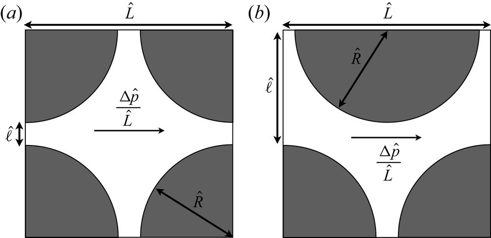
Figure 10. Schematic of the model porous media: (a) regular geometry, (b) staggered geometry.
Figure 11 compares different flows within a wide range of Bingham numbers. Dead zones (shaded in light grey) are smaller in the sliding flows since the fluid slides over the solid surfaces and ‘erodes’ the fouling parts. However, the unyielded regions in the middle of the passage (yield surfaces in green) are mostly larger compared with the no-slip condition, which is intuitive. Interestingly, because of the slip, unyielded zones are prone to attach to the solid surfaces (e.g. see figure 11p).
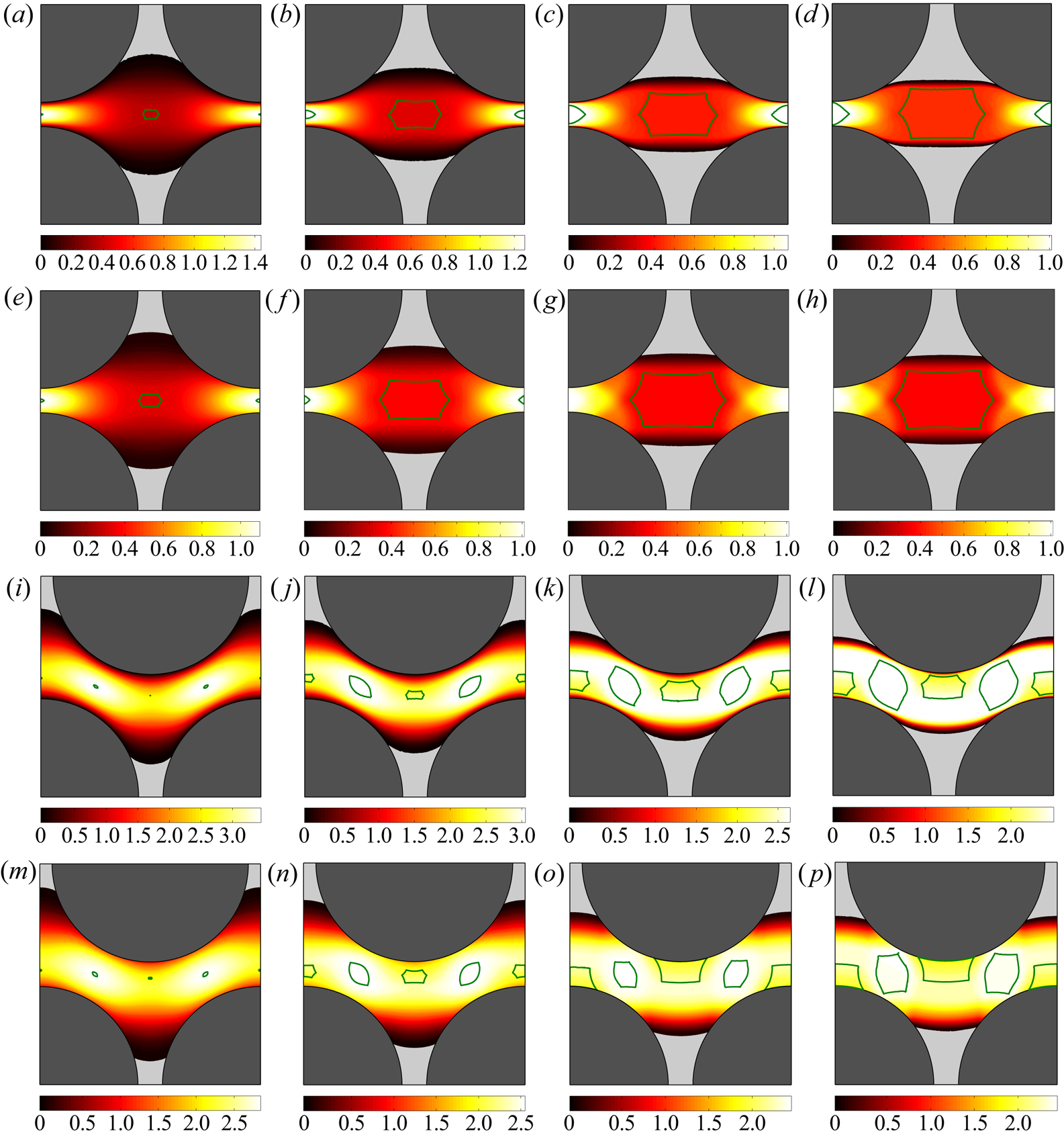
Figure 11. The velocity magnitude contour  $\vert \boldsymbol {u}^* \vert$. Panels (a–d) and (i–l) show the no-slip flow in the regular and staggered geometries, respectively. Panels (e–h) and (m–p) illustrate the sliding flow ( $\alpha _s=0.2,\beta _s=0.1$) in regular and staggered geometries, respectively. Panels (a,e,i,m), (b,f,j,n), (c,g,k,o) and (d,h,l,p) are associated with $B=1$, 10, 100 and 1000, respectively. The dead zones are shown in light grey and green lines represent the yield surfaces in the middle of the flow passage.
Figure 12 reveals, quantitatively, various features of the flow in the model porous media. Figure 12(a) sketches  $G^*$ with respect to the Bingham number; zoomed-in insets are provided in figure 12(b–e). In the range of small Bingham numbers – Newtonian limit – the pressure gradient is a function of $B$ and $\beta _s$ alone; see figures 12(b) and 12(d) in which the cyan and yellow curves ( $\beta _s = 0.05$) converge together and also red and purple curves ( $\beta _s = 0.1$) together. On the other hand, in the limit of large Bingham numbers (i.e. no flow or yield limit; figures 12c and 12e), the critical pressure gradient is a function of $B$ and $B_s$ or indeed $B$ and $\alpha _s$: yellow and red curves with $\alpha _s=0.2$ are almost indistinguishable; the same for the purple and cyan curves with $\alpha _s=0.8$. Moreover, as shown by Chaparian et al. (Reference Chaparian, Izbassarov, De Vita, Brandt and Tammisola2020), in the yield limit ( $B \to \infty$), the pressure gradient scales with ${\sim }B$; this is true for both the no-slip and sliding flows, yet with different prefactors. Indeed, as shown in § 3.2 for the simple channel flow,
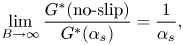 \begin{equation} \lim_{B \to \infty} \frac{G^*(\text{no-slip})}{G^*(\alpha_s)}=\frac{1}{\alpha_s}, \end{equation}
which is the case in the complex flows through model porous media as well.
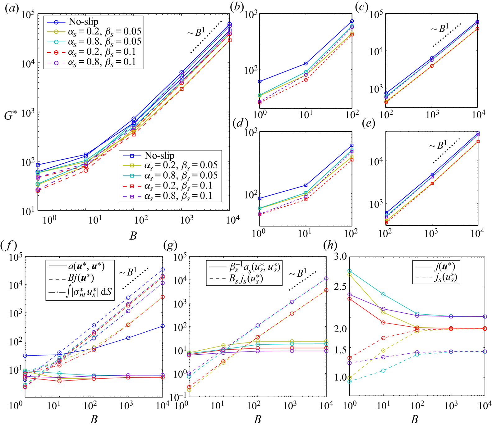
Figure 12. Features of the flow in model porous media: (a)  $G^*$ versus $B$, the circles stand for the regular geometry and squares for the staggered cases; (b,c) close-up of the panel (a) at small and large Bingham numbers, respectively (only data of the regular geometry is presented); (d,e) close-up of the panel (a) at small and large Bingham numbers, respectively (only data of the staggered geometry is presented); (f) different contributions to the total dissipation versus the Bingham number; (g) different contributions to the slip dissipation versus the Bingham number; (h) normalized plastic dissipation and ‘plastic’ slip dissipation versus $B$. The scale of the vertical axis in this panel is not logarithmic – it is linear. Please note that in panels (f–h) only data of the regular geometry is presented and the colour interpretation is the same as in panel (a).
Figure 12(f) confirms that the viscous dissipation, even in sliding flows, is at least one order of magnitude less than the plastic and slip dissipations. Interestingly, for sliding flows,  $a(\boldsymbol {u}^*,\boldsymbol {u}^*)$ converges to its limiting value when $B \to \infty$ and the limiting value is a function of $\alpha _s$ only. Whereas, in the no-slip flow, the viscous dissipation increases by increasing Bingham number but with a much smaller rate compared with the plastic dissipation. Figure 12(f) also shows that the leading-order dissipation terms (i.e. $Bj(\boldsymbol {u}^*)$ and $\int \vert \sigma ^*_{nt} u^*_s \vert \,\text {d}S$) scales with ${\sim } B$ at the yield limit for sliding flows which is the main reason of yielding to the same scaling for $G^*$ at this limit – see (3.13). Figure 12(g) also establishes that the leading-order term in the slip dissipation is the ‘plastic’ slip dissipation $B_s j_s(u^*_s)$.
Please note that although  $j(\boldsymbol {u}^*)$ of the no-slip flow is not shown in figure 12(h), the trend is the same as the sliding flows, but of course with larger values as it is clear from figure 12(f) where $Bj(\boldsymbol {u}^*)$ is shown.
Under the no-slip condition, the asymptotic values of  $j(\boldsymbol {u}^*)$ at $B \to \infty$ are equal to $3.42$ and $12.57$ for regular and staggered geometries which yield to $Od_c = {\hat {\tau }_y}/{\hat {R} \hat {G}_c} \approx 0.1645$ and ${\approx } 0.2237$, respectively, using (3.14) in the absence of any slip dissipation. The critical Oldroyd number in the presence of slip is calculated using the same expression in table 1. Please note that as an approximation, one may alternatively use
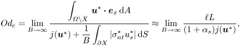 \begin{equation} Od_c = \lim_{B \to \infty} \frac{\displaystyle \int_{\varOmega \setminus \bar{X}} \, \boldsymbol{u}^* \boldsymbol{\cdot} \boldsymbol{e}_x \,\text{d}A}{j(\boldsymbol{u}^*)+\displaystyle \frac{1}{B} \int_{\partial X} \vert \sigma^*_{nt} u^*_s \vert \,\text{d}S} \approx \displaystyle \lim_{B \to \infty} \frac{\ell L}{(1+\alpha_s)j(\boldsymbol{u}^*)}, \end{equation}
in which  $j_s(u_s^*)$ is approximated by $j(\boldsymbol {u}^*)$ as is suggested by figure 12(h), especially for small values of $\alpha _s$ (i.e. more slippery flows). These values are reported in table 1 as well. A negligible difference between $Od_c$ calculated using (3.14) and (5.2) for $\alpha _s=0.2$ shows the validity of this approximation when the ‘sliding yield stress’ is much smaller than the material yield stress.
Table 1. Values of  $Od_c$ for regular and staggered geometries.
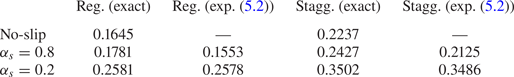
We shall mention that, as it is clear from figure 12(c,e,h),  $Od_c$ only depends on $\alpha _s$ as reported in table 1 (at least for $0 \leqslant \beta _s \leqslant 0.1$).
6. Towards more complex geometries
Although previous studies on the yield-stress fluid flows in the model porous media uncovered some generic interesting aspects of the problem, yet they were not capable of capturing the whole physics behind these type of complex flows. For instance, Talon & Bauer (Reference Talon and Bauer2013) utilized the lattice Boltzmann method (known as LBM) to study the Bingham fluid flow in a stochastically reconstructed porous media. These authors showed that due to the yield stress, channelization can happen: the material will flow only in self-selected paths depending on the imposed driving pressure gradient; at the yield limit it is only one path and by increasing the pressure gradient gradually, other paths will open up. This has been supported by the work of Liu et al. (Reference Liu, De Luca, Rosso and Talon2019) in model pore networks connected by straight tubes.
To capture these kinds of fascinating and more realistic behaviours, in this section we will complement the findings in § 5 by studying the flow in random-designed porous media with a wide range of porosities. The computational domain is a box of dimensions  $50 \times 50$ where the fluid flows around 2-D fixed rigid circles of radius unity with symmetric boundary conditions on the pair of the horizontal and vertical box faces. Again we use the [R] formulation in this section and the same numerical method as in the previous section. To have a better comparison, in addition to the random porous media, we simulate the flow again in the two introduced model porous media (figure 10); yet with the same porosity as the random cases: the size of the model cell in figure 10 is $L=\sqrt {{{\rm \pi} }/{1-\phi }}$.
6.1. Baseline no-slip flow
Figure 13 illustrates the no-slip flow in the case  $\phi = 0.7$ for a wide range of Bingham numbers from unity to $10^4$. Panels (a,b), (c) show the velocity magnitude contours and panels (d,e), (f) the logarithmic scale of the second invariant of the rate of strain tensor. When the Bingham number increases, the flow becomes more and more localized, and at the yield limit ( $B \to \infty$), the flow only passes through a single channel. Please note that the black level contours represent the quiescent parts. It is worth mentioning that due to the [R] scaling, the flow rate in all the simulations is the same (for a fixed geometry regardless of the Bingham number, $\alpha _s$ and $\beta _s$), hence, in figure 13(c) the whole fluid passes through the single open channel which results in extremely high velocities (compare the level of contours in the panels (a,b), (c)). By looking at the panels from left to right sequentially, the channelization characteristic is clearly observable: by increasing the Bingham number (i.e. moving to the yield limit), the flow occurs in lesser paths, until only one path remains at the yield limit.
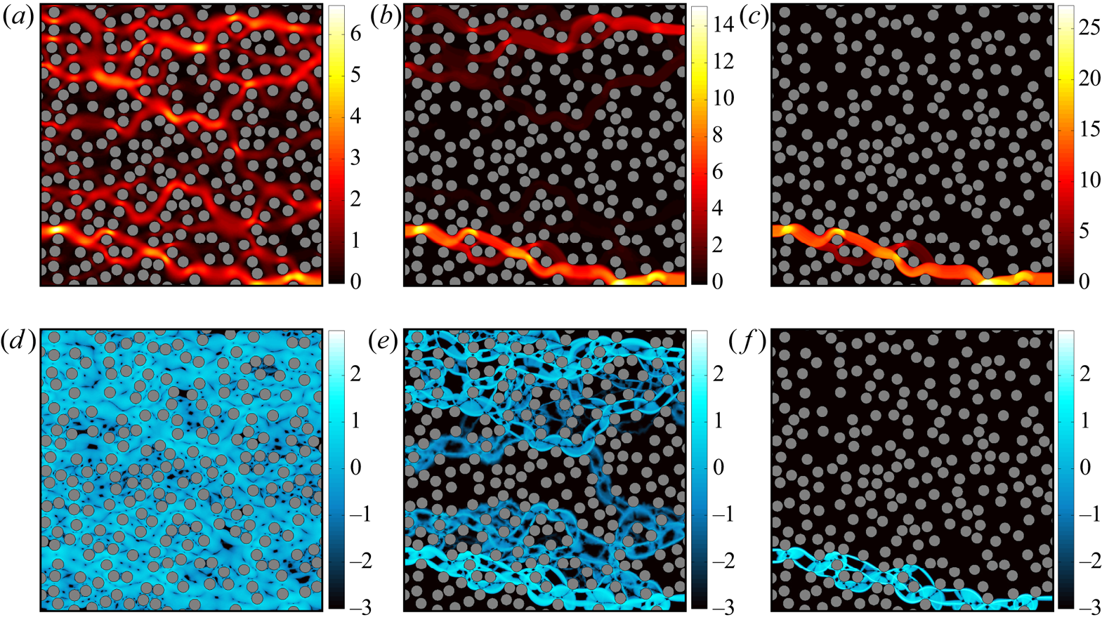
Figure 13. Here  $\phi =0.7$ where panels (a–c) illustrate $\vert \boldsymbol {u}^* \vert$ and (d–f) contour of $\log _{10} (\Vert \dot {\boldsymbol {\gamma }}^* \Vert )$ for flows with no-slip condition. Please note that the range of colourbars are different in velocity contours whereas it is the same in panels (d–f). Panels (a,d), (b,e) and (c,f) are associated with $B=1$, 100 and $10^4$, respectively.
Figure 14 shows the pressure drop against the Bingham number. The lines are computed data in the present study and the symbols are computational and experimental data by Bauer et al. (Reference Bauer, Talon, Peysson, Ly, Batôt, Chevalier and Fleury2019) for three-dimensional (3-D) flows. The blue lines are acquired from the randomized porous media and the red lines from the two model porous media for a wide range of porosities. To have a better comparison, we combined  $G^*$ from the regular and staggered models in the red lines by averaging. This figure demonstrates that the model porous media closely predicts the pressure drop in the randomized porous media, however, there are small discrepancies, more pronounced in the two limits of the problem – Newtonian and the yield limit. Yet, in the intermediate regime of the Bingham numbers, the predictions are more satisfactory. Table 2 compares the critical Oldroyd number under the no-slip condition computed in different configurations. As can be seen in figure 14, the model porous media slightly overpredicts the pressure drop which results in smaller $Od_c$ compared with the randomized geometries.
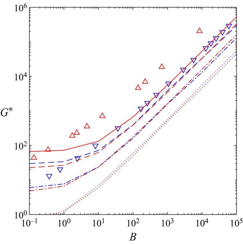
Figure 14. Pressure drop with respect to the Bingham number under the no-slip condition. The red colour stands for simulations of the model porous media and the blue colour the simulations of the random porous media. The lines represent our computations: the continuous line corresponds to  $\phi =0.38$, dashed line to $\phi =0.5$, dashed-dotted line to $\phi =0.7$ and the dotted line to $\phi =0.9$. The symbols are data borrowed from Bauer et al. (Reference Bauer, Talon, Peysson, Ly, Batôt, Chevalier and Fleury2019): simulations for face-centred cubic packing of spheres ( $\vartriangle$, $\phi =0.218$), simulations for random array of overlapping spheres ( $\triangledown$, $\phi =0.429$).
Table 2. Comparison of  $Od_c$ (under no-slip condition) for different geometries.
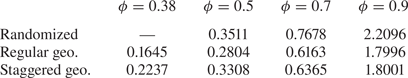
In figure 14, we also compare 2-D simulations in the present study and 3-D simulations by Bauer et al. (Reference Bauer, Talon, Peysson, Ly, Batôt, Chevalier and Fleury2019). They are partially comparable; specifically in the large Bingham number limit where a large portion of domain is filled with static/fouling regions. However, a closer comparison in the Newtonian limit is suggestive of different trends, which could be the consequence of different flow structures in 2-D and 3-D flows in this limit and also the difference between the viscous functionality in the Bingham model which is used here and the Herschel–Bulkley model used by Bauer et al. (Reference Bauer, Talon, Peysson, Ly, Batôt, Chevalier and Fleury2019). More sophisticated analyses/comparisons of the model and random porous media under the no-slip condition are presented in appendix B, as the main focus of the present study is on the sliding flows.
6.2. Effect of slip
In this subsection, we take a close look at the effect of slip in the randomized porous media. Figures 15 and 16 compare the velocity and the rate of strain fields, respectively, between the flows under the no-slip condition and the sliding flows ( $\alpha _s=0.2\ \&\ \beta _s=0.1$) at $B=10^4$. These two figures show that when the flow can slide over the pores’ surfaces, the channelization is not strong compared with the no-slip condition. Indeed, the flow slides over the solid surfaces which cover a large portion of the domain in the small porosities limit and consequently there is a flow in most of the passages. However, in the limit of high porosities (i.e. less solid surfaces), the effect of slip is negligible: compare panels (c) and (f) in figures 15 and 16. The static regions under the no-slip condition and in the sliding flows are almost the same when porosity is as high as $\phi =0.9$. There are slightly sheared parts out of the main open path (see figure 16f), but the flow mainly passes through the open channel whose shape and location are identical to the no-slip case.
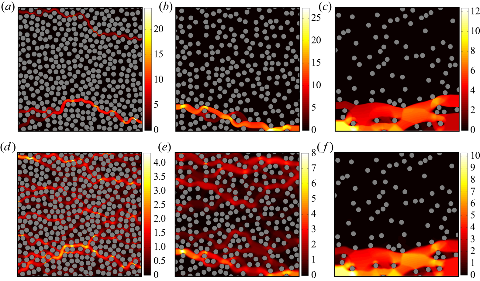
Figure 15. Here  $\vert \boldsymbol {u}^* \vert$ at $B=10^4$ for (a–c) no-slip flow, (d–f) sliding flow ( $\alpha _s=0.2$ and $\beta _s=0.1$). Panels (a,d), (b,e) and (c,f) correspond to $\phi =0.5$, 0.7 and 0.9, respectively.
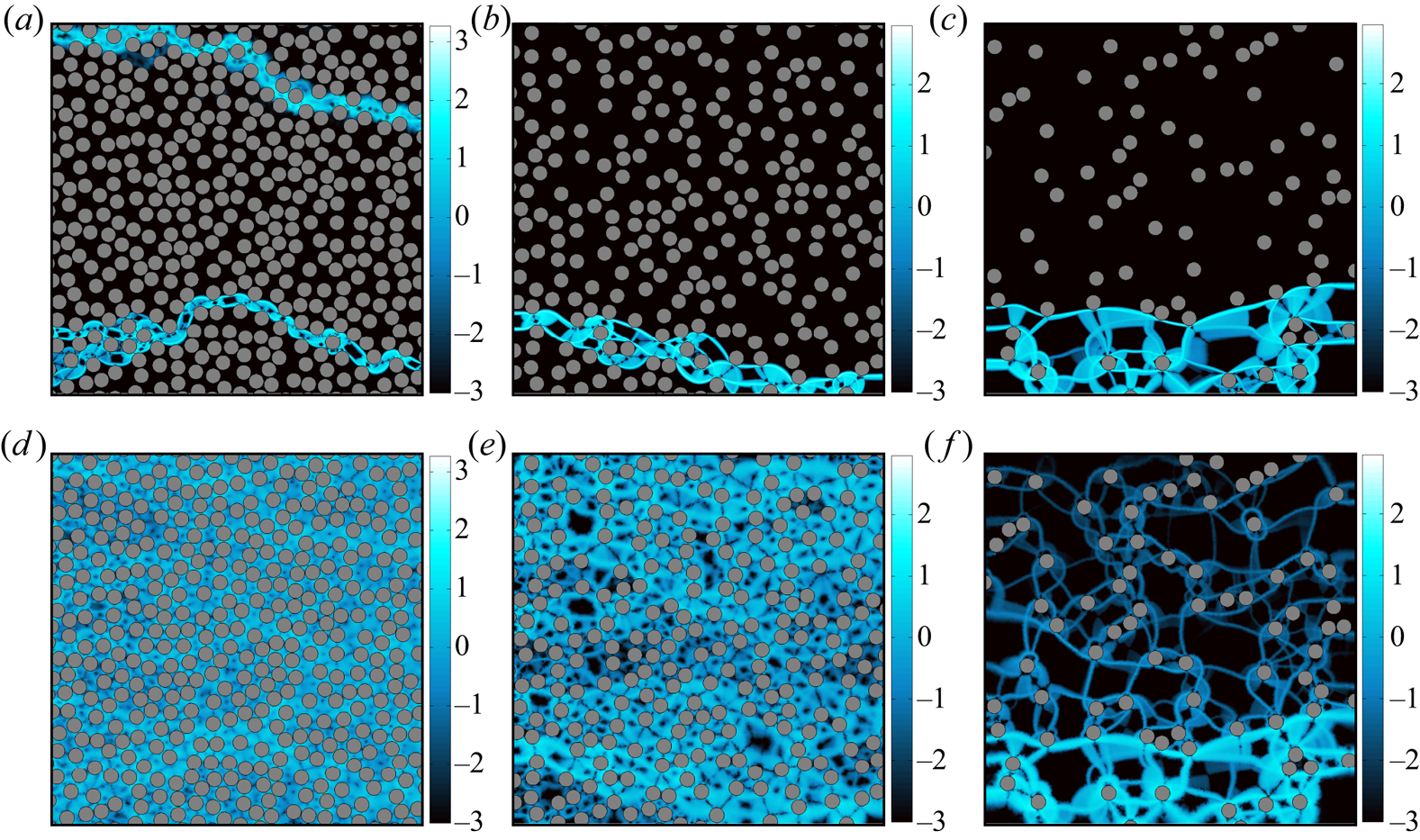
Figure 16. Here  $\log _{10} ( \Vert \dot {\boldsymbol {\gamma }}^* \Vert )$ at $B=10^4$ for (a–c) no-slip flow, (d–f) sliding flow ( $\alpha _s=0.2$ and $\beta _s=0.1$). Panels (a,d), (b,e) and (c,f) correspond to $\phi =0.5$, 0.7 and 0.9, respectively. Please note that for each row, we have used the same range of colourbar.
Figure 17 looks at this phenomenon from the pressure drop perspective. The lines (no-slip simulations) are borrowed from figure 14 for reference. The symbols refer to sliding flows ( $\alpha _s=0.2\ \&\ \beta _s=0.1$); the blue ones collected from the simulations in the randomized porous media and the red ones from the model porous media. Please note that again we plot the average value of $G^*$ corresponding to the two model porous media (normal and staggered cases). This figure demonstrates that as the porosity increases, the effect of slip on the pressure drop decreases, in agreement with figures 15 and 16 for the model porous media. Indeed, the symbols are much closer to their corresponding lines with the same porosity as $\phi \to 1$. Moreover, in this high porosity limit, the model porous media predictions are appropriate approximations of the pressure drop in the randomized porous media: the asterisks and pluses with different colours are not distinguishable. However, in the other limit (low porosities), the effect of slip on the pressure drop is more pronounced: the pressure drop in the sliding flows are smaller compared with no-slip flows, which is intuitive. Moreover, the intensity of the slip effect on the pressure drop depends on the geometric structures since there is a significant discrepancy between the predictions of the model porous media and the randomized porous media: the blue and red full circles are relatively far from each other specifically in the low Bingham number regime (please note the logarithmic scale).
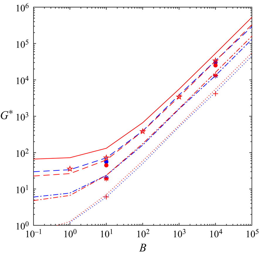
Figure 17. Pressure drop with respect to the Bingham number. The red colour stands for the simulations of the model porous media and blue colour the simulations of the random porous media. The lines are borrowed from figure 14 (no-slip condition): the continuous line corresponds to  $\phi =0.38$, dashed line to $\phi =0.5$, dashed-dotted line to $\phi =0.7$ and the dotted line to $\phi =0.9$. The symbols are computations of the sliding flow ( $\alpha _s=0.2\ \&\ \beta _s=0.1$): stars correspond to $\phi =0.38$, full circles to $\phi =0.5$, asterisks to $\phi =0.7$ and the pluses to $\phi =0.9$.
7. Summary and discussion
The hydrodynamic features of sliding flows of yield-stress fluids are investigated in the present study. It has been well-documented in the literature that yield-stress fluids slide over solid surfaces due to microscopic effects: formation of a lubrication layer of solvent and elastic deformation of soft particles in the vicinity of the solid surface (Meeker et al. Reference Meeker, Bonnecaze and Cloitre2004b). Firstly, we formulated a general vectorial form of the well known ‘stick–slip’ law and presented a numerical algorithm based on the augmented Lagrangian scheme combined with anisotropic mesh adaptation to attack these kinds of problems. We derived some theoretical tools as well to formulate the yield limit in the presence of slip. The whole framework was benchmarked in a simple channel Poiseuille flow. Then we addressed more complicated problems including moving solid surfaces and the sliding flow over complex topologies.
Firstly, we simulated the slippery particle sedimentation problem and addressed the yield limit in detail. Slipline solutions from the perfectly plastic mechanics were revisited and utilized to find the yield limit in the presence of slip. The slipline method has proved capable of finding the yield limit, even though the velocity/stress fields obtained from slipline solutions can differ from the viscoplastic solutions at large, yet finite Bingham numbers – see Chaparian & Frigaard (Reference Chaparian and Frigaard2017b). The conclusions from the present study are similar, showing again that the lower and upper bounds of the plastic drag coefficient are excellent estimations of the yield limit of slippery particle motion.
Secondly, we addressed the complex sliding flows in the model and randomized porous media. Different hydrodynamic features of the flow were investigated as well as the critical pressure gradient to ensure continuous non-zero flow was reported. Moreover, some general conclusions were drawn about modelling the flow in porous media by comparing the results computed from the model configurations and more realistic random-designed porous media, both under the no-slip condition and sliding flows. Furthermore, it was shown that the effect of slip is more severe in the low porosity limit where a larger portion of the domain is filled by occupying solids (i.e. a large portion of the flow is in contact with the solid surfaces). In this limit, the pressure drop of a slippery flow is decreased compared with the flow under the no-slip condition. For instance, the pressure drop under the no-slip condition at  $\phi =0.5$ closely follows the pressure drop of the sliding flow for the case $\phi =0.38$ when $\alpha _s=0.2~\&~\beta _s=0.1$ (see figure 17). Indeed, an effective porosity can be defined for the sliding flows in porous media to predict the pressure drop: $G^* (\phi _{eff}; \text {no-slip}) = G^* (\phi; \alpha _s, \beta _s)$ where $\phi _{eff} > \phi$. In the high porosity limit, however, $\phi _{eff} \approx \phi$ since the solid surfaces are occupied by a small portion of the whole domain.
By investigating different physical problems in the presence of slip, from particle motion to pressure-driven flows in complex geometries, the following general conclusions can be drawn about sliding flows of viscoplastic fluids.
(i) There are three sources of dissipation in sliding flows: viscous, plastic and slip dissipations. Slip dissipation itself can be split into two main contributions: ‘viscous’ slip dissipation which comes from the slip coefficient
$\beta _s$ and ‘plastic’ slip dissipation which is the contribution of the sliding yield stress.(ii) In the yield limit, the leading-order contribution to the total slip dissipation is the ‘plastic’ slip dissipation. Exploiting that viscous dissipation is at least one order of magnitude less than the plastic dissipation, we can conclude that the yield limit of sliding flows is indeed controlled by
$\alpha _s$ or sliding yield stress. This was evidenced both for particle sedimentation and pressure-driven flows in porous media.(iii) In the other limit (Newtonian limit), however, the flow characteristics are determined by the slip coefficient
$\beta _s$. For instance, the plastic drag coefficient in the particle sedimentation problem and the pressure drop in the porous media are the same for the flows with the same $\beta _s$ as $B \to 0$.


Finally, we should mention that, although in the entire study we considered  $k=1$ and the Bingham model as the rheological representation, the presented framework and most of the conclusions that are drawn are independent of these assumptions. In appendix C, we will show how we can adopt the presented numerical algorithm and the analytical tools to study the cases in which $k \neq 1$ and $n \neq 1$.
Acknowledgements
E.C. gratefully acknowledges the Linné FLOW PostDoc grant during the course of this study.
Funding
The authors appreciate the support of Swedish Research Council through grant VR 2017-0489. This project also has received funding from the European Research Council (ERC) under the European Union's Horizon 2020 research and innovation programme (grant agreement no. 852529).
Declaration of interests
The authors report no conflict of interest.
Appendix A. Analytical solution of the sliding Poiseuille flow
We derive analytical solutions for the sliding Poiseuille flow in a channel with gap width unity considering both [M] and [R] formulations.
A.1. The [M] problem
For the [M] problem, the only non-zero stress component is the shear stress which can be derived from
 \begin{equation} \frac{\text{d}\tau_{xy}}{\text{d}y} = 1, \end{equation}
and the slip velocity can be calculated from
 \begin{equation} u_{{s}} = \left\{ \begin{array}{@{}ll} \beta_s \left( \vert \tau_w \vert - Od_s \right), & \text{iff}\ \vert \tau_{w} \vert > Od_s, \\ 0, & \text{iff}\ \vert \tau_{w} \vert \leqslant Od_s, \end{array} \right. \end{equation}
where  $\tau _w$ is the wall shear stress. From the constitutive equation, we know that in the yielded regions (if there are any),
 \begin{equation} Od \,\text{sgn}(y)-y=\dot{\gamma}_{xy}=\frac{\text{d}u}{\text{d}y}. \end{equation}
Hence, if  $\vert y \vert \geqslant Od$,
 \begin{equation} u = Od\vert y \vert-\frac{y^2}{2} + A, \end{equation}
with the boundary condition,
 \begin{equation} u\left(y=\pm \frac{1}{2}\right) = u_s = \beta_s \left(\frac{1}{2} - Od_s \right). \end{equation}
 Therefore, three different scenarios can happen based on values of  $Od$ and $Od_s$, namely
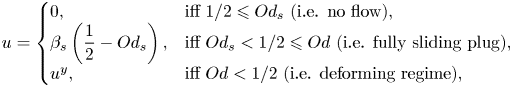 \begin{equation} u = \left\{ \begin{array}{@{}ll} 0, & \text{iff}\ 1/2 \leqslant Od_s ~\text{(i.e. no flow)}, \\ \beta_s \left(\dfrac{1}{2} - Od_s\right), & \text{iff}\ Od_s < 1/2 \leqslant Od\ \text{(i.e. fully sliding plug)}, \\ u^y, & \text{iff}\ Od < 1/2\ \text{(i.e. deforming regime)}, \end{array} \right. \end{equation}
where,
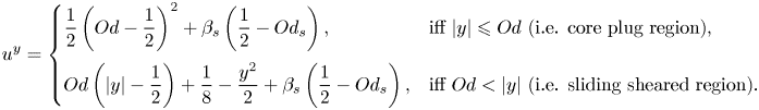 \begin{equation} u^y = \left\{ \begin{array}{@{}ll} \dfrac{1}{2} \left( Od - \dfrac{1}{2} \right)^2 + \beta_s \left( \dfrac{1}{2} - Od_s \right), & \text{iff}\ \vert y \vert \leqslant Od\ \text{(i.e. core plug region)}, \\ Od\left(\vert y \vert -\dfrac{1}{2}\right) + \dfrac{1}{8} - \dfrac{y^2}{2} + \beta_s \left(\dfrac{1}{2} - Od_s\right), & \text{iff}\ Od < \vert y \vert\ \text{(i.e. sliding sheared region)}. \end{array} \right. \end{equation}
Hence,  $Od_c = 1 / 2 \alpha _s$.
A.2. The [R] problem
In the [R] formulation, we always have a non-zero flow rate due to the velocity scaling. Hence, we shall identify two different regimes: deforming regime at small and moderate Bingham numbers ( $B < \bar {B}$) and a fully sliding plug at $B \to \infty$ (or strictly when $B > \bar {B}$). The shear stress satisfies
 \begin{equation} \frac{\text{d}\tau^*_{xy}}{\text{d}y^*} = G^*, \end{equation}
with the slip velocity,
 \begin{equation} u_s^* = \left\{\begin{array}{@{}ll} \beta_s \left( \vert \tau^*_{w} \vert - B_s \right), & \text{iff}\ \vert \tau_w^* \vert > B_s, \\ 0, & \text{iff}\ \vert \tau_w^* \vert \leqslant B_s. \end{array} \right. \end{equation}
In the deforming regime, in the yielded regions,
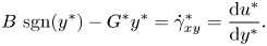 \begin{equation} B ~\text{sgn} (y^*)-G^* y^*=\dot{\gamma}^*_{xy}=\frac{\text{d}u^*}{\text{d}y^*}. \end{equation}
Hence,
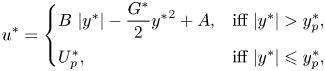 \begin{equation} u^* = \left\{ \begin{array}{@{}ll} B~\vert y^* \vert - \dfrac{G^*}{2} {y^*}^2 + A, & \text{iff}\ \vert y^* \vert > y^*_p, \\ U_p^*, & \text{iff}\ \vert y^* \vert \leqslant y^*_p, \end{array} \right. \end{equation}
where  $y^*_p = {B}/{G^*}$ and $u(y^*_p) = U^*_p$. The boundary condition for velocity is
 \begin{equation} u^* \left( \pm \frac{1}{2} \right) = u_s^* = \frac{\beta_s G^*}{2} \left( 1 - \frac{2 B_s}{G^*} \right), \end{equation}
therefore,
 \begin{equation} u^* = \left\{ \begin{array}{@{}ll} B\left( \vert y^* \vert - \displaystyle\dfrac{1}{2} \right) + \displaystyle\dfrac{G^*}{2} \left[ \dfrac{1}{4} - {y^*}^2 + \beta_s \left( 1-\dfrac{2 B_s}{G^*} \right) \right], & \text{iff}\ \vert y^* \vert > y^*_p, \\ U^*_p, & \text{iff}\ \vert y^* \vert \leqslant y^*_p. \end{array} \right. \end{equation}
Please note that still  $G^*$ is unknown and should be calculated from continuity
 \begin{equation} 1 = 2 \int_0^{1/2} u^* \,\text{d}y^* = G^* \left( \frac{1}{12} + \frac{\beta_s}{2} \right) + B \left( \frac{B^2}{3~{G^*}^2} - \frac{1}{4} \right) - \beta_s B_s. \end{equation}
The individual dissipation terms can be calculated as
 \begin{gather} a(\boldsymbol{u}^*,\boldsymbol{u}^*) = \int_{-1/2}^{1/2} \left( \frac{\text{d}u^*}{\text{d}y^*} \right)^2 \text{d}y^* = \frac{2}{3G^*} \left( \frac{G^*}{2} - B \right)^3, \end{gather}
 \begin{gather}B j(\boldsymbol{u}^*) = \int_{-1/2}^{1/2} \left\vert \frac{\text{d}u^*}{\text{d}y^*} \right\vert \text{d}y^* = B \left( \frac{G^*}{4} - B + \frac{B^2}{G^*} \right) \end{gather}
and
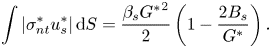 \begin{equation} \int \vert \sigma_{nt}^* u_s^* \vert \,\text{d}S = \frac{\beta_s {G^*}^2}{2} \left( 1 - \frac{2 B_s}{G^*} \right). \end{equation}
However, in the case of fully sliding plug, the slip velocity is
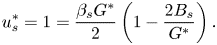 \begin{equation} u_s^* = 1 = \frac{\beta_s G^*}{2} \left( 1 - \frac{2 B_s}{G^*} \right). \end{equation}
Hence,
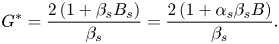 \begin{equation} G^* = \frac{2 \left( 1 + \beta_s B_s \right)}{\beta_s} = \frac{2 \left( 1 + \alpha_s \beta_s B \right)}{\beta_s} . \end{equation}
Therefore, the critical Bingham number beyond which the fully sliding plug occurs is
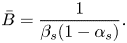 \begin{equation} \bar{B} = \frac{1}{\beta_s (1-\alpha_s)}. \end{equation}
Appendix B. Flow rate curve in porous media
Bauer et al. (Reference Bauer, Talon, Peysson, Ly, Batôt, Chevalier and Fleury2019) considered 3-D flow in model and random porous media using a regularized lattice–Boltzmann approach. The model geometry used was a face-centred cubic maximum-packing arrangement of spheres whereas, a random array of overlapping spheres was designed for more realistic porous media. Interestingly, Bauer et al. (Reference Bauer, Talon, Peysson, Ly, Batôt, Chevalier and Fleury2019) reported that the model and random porous media display different flow rate dependencies: i.e. flow rate ( ${\sim } B^{-1}$) as a function of the excessive pressure gradient ( ${\sim } Od^{-1} - Od_c^{-1}$) or
 \begin{equation} B^{-1} \sim \left( Od^{-1} - Od_c^{-1} \right)^{\zeta}. \end{equation}
They observed that the model porous media predicts a single scaling  $\zeta \approx 2$ while the random porous media exhibits two distinctive scalings in the range of moderate and low/high excessive pressure gradients. In other words, in random porous media, both viscous limit and yield (i.e. plastic) limit share similar characteristics/slopes in predicting the flow rate as a function of the excessive pressure gradient ( $\zeta \approx 2$). However, in the viscoplastic regime, the slope is higher ( $\zeta \approx 3$). This has been proved by experimental data collected by considering Carbopol flow through a sandstone bed.
Using the computational data of the present study under the no-slip condition, we consider how the 2-D model porous media and the 2-D randomized porous media predict the flow rate curves and how it differs from the simulations/experiments of Bauer et al. (Reference Bauer, Talon, Peysson, Ly, Batôt, Chevalier and Fleury2019). Moreover, we investigate if the model and randomized porous media share the same characteristics in converging to the yield limit at large  $B$.
$B$.
Figure 18(a) illustrates the convergence to the yield limit ( $1-{Od}/{Od_c}$) versus the Bingham number. All the simulations display more or less the same scalings,
 \begin{equation} 1-\frac{Od}{Od_c} \sim B^{-\nu}, \end{equation}
where  $\nu \approx -1$. However, two more conclusions can be drawn from figure 18(a).
(i) At small porosities, we need to go to the higher Bingham numbers to get close enough to the yield limit. This can be attributed to the highly localized and heterogeneous/channelized flow at small porosities. Data borrowed from Bauer et al. (Reference Bauer, Talon, Peysson, Ly, Batôt, Chevalier and Fleury2019) also show the same characteristics, yet a slower convergence rate (
$\vert \nu \vert < 0.9$) with the Bingham number compared with our results, which could be the consequence of 3-D flows.(ii) At high porosities, the model and randomized porous media display closely matched convergence to the yield limit by increasing the Bingham number. For instance, see the dotted blue line (randomized) and the two dotted red lines decorated with symbols (regular and staggered models with circles and squares). However, at the low porosities, the model porous media displays faster convergence compared with the randomized porous media (compare the red continuous lines and symbols (
$\phi =0.38$) with the dashed line ($\phi =0.5$)).


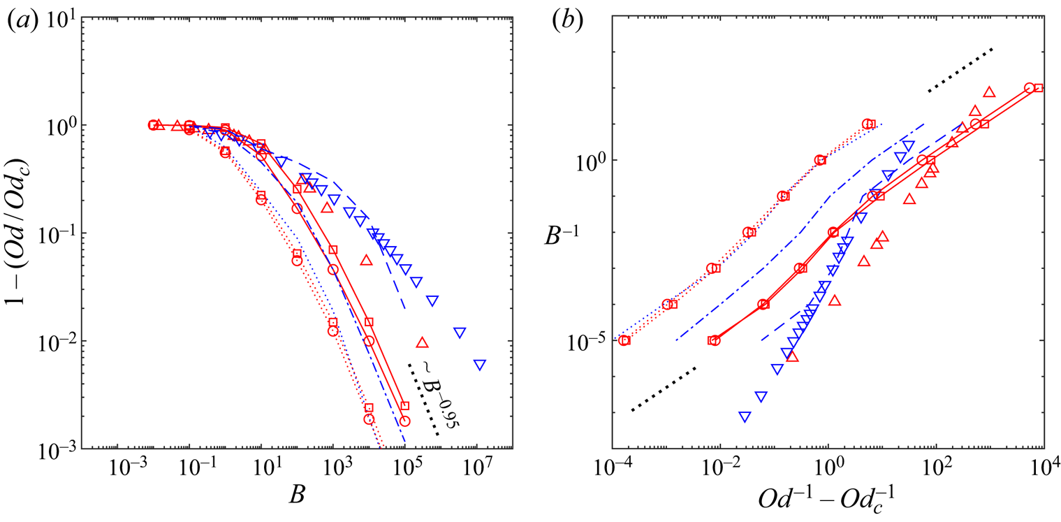
Figure 18. Flow features in model and random-designed porous media. The lines and symbols interpretation is the same as figures 14 and 17. Please note that in both panels, the lines with circles correspond to the regular model geometry (figure 10a) and those with squares to the staggered model geometry (figure 10b). The dotted black line in panel (a) marks  $B^{-0.95}$ scaling and the two dotted black lines in panel (b) 1 : 1 scaling for reference.
Another interesting feature to compare, as discussed above, is the flow rate curve – see figure 18(b) which shows the flow rate versus the excessive pressure gradient. Contradictory to what has been reported by Bauer et al. (Reference Bauer, Talon, Peysson, Ly, Batôt, Chevalier and Fleury2019), this figure shows that the model porous media (at least in two dimensions), predicts same behaviour: in the sense that at small and large excessive pressure gradients (yield and Newtonian limits, respectively), the flow rate scales linearly with the excessive pressure gradient; however, at the intermediate regime, the flow rate growth as a function of  ${1}/{Od}-{1}/{Od_c}$ is faster. This behaviour is manifested by the randomized porous media as well. Though, as is clear from figure 18(b), $\zeta$ is different in our data from the one reported by Bauer et al. (Reference Bauer, Talon, Peysson, Ly, Batôt, Chevalier and Fleury2019). Indeed, both Bauer et al. (Reference Bauer, Talon, Peysson, Ly, Batôt, Chevalier and Fleury2019) and Chevalier et al. (Reference Chevalier, Chevalier, Clain, Dupla, Canou, Rodts and Coussot2013) demonstrated that $\zeta$ is close to the inverse of the power-law index of the Herschel–Bulkley fluid, $\zeta \approx 1/n$. Considering that in the present problem we have used the Bingham model ( $n=1$), it makes sense why we found a different exponent ( $\zeta \approx 1$) which is consistent with the $\zeta \approx 1/n$ discussion.
Appendix C. Extensions to the non-ideal cases: $k \neq 1$ and $n \neq 1$


In the main analyses throughout the paper, we have assumed that  $k=1$. As discussed in §§ 1 and 2, this assumption is founded on many experimental observations. However, in this appendix, we intend to expand our understanding for the cases in which $k \neq 1$, and also non-ideal viscoplastic rheology. In the resolution of the presented numerical method, ‘simple’ viscoplastic models can be easily adopted such as Herschel–Bulkley and Casson models: step 7 needs updating in the presented algorithm, which is clearly explained by Huilgol & You (Reference Huilgol and You2005). For instance, for the Herschel–Bulkley model, it takes the form
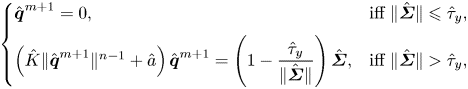 \begin{equation} \left\{\begin{array}{@{}ll} \hat{\boldsymbol{q}}^{m+1}=0, & \text{iff}\ \Vert \hat{\boldsymbol{\varSigma}} \Vert \leqslant \hat{\tau}_y, \\ \left( \hat{K} \Vert \hat{\boldsymbol{q}}^{m+1} \Vert^{n-1} + \hat{a} \right) \hat{\boldsymbol{q}}^{m+1} = \left( 1- \displaystyle\dfrac{\hat{\tau}_y}{\Vert\hat{\boldsymbol{\varSigma}}\Vert} \right) \hat{\boldsymbol{\varSigma}}, & \text{iff}\ \Vert \hat{\boldsymbol{\varSigma}} \Vert > \hat{\tau}_y, \end{array} \right. \end{equation}
where  $\hat {\boldsymbol {\varSigma }} = \hat {\boldsymbol {T}}^m+\hat {a} \,\hat {\dot {\boldsymbol {\gamma }}} (\hat {\boldsymbol {u}}^{m+1})$. In the case of more complex models, e.g. elastoviscoplastic models, one needs more effort – please see Chaparian & Tammisola (Reference Chaparian and Tammisola2019).
In the following, as an example, we consider the 2-D circular Couette flow between two infinitely long cylinders of radii  $\hat {R}_1$ and $\hat {R}_2$ – see figure 19. We consider this specific geometry to compare our numerical results with the experimental measurements reported by Medina-Bañuelos et al. (Reference Medina-Bañuelos, Marín-Santibáñez, Pérez-González, Malik and Kalyon2017): they reported the velocity profiles in the gap using rheo-particle image velocimetry measurements and also slip laws on the cylinder surfaces for a Carbopol microgel 0.12 wt. % with the rheological properties $\hat {\tau }_y = 27\ \textrm {Pa}$, $\hat {K}=5.5\ \textrm {Pa}.s^n$ and $n=0.43$. Figure 19(b) compares our numerically obtained velocity profiles (red lines) with the experimental measurements of Medina-Bañuelos et al. (Reference Medina-Bañuelos, Marín-Santibáñez, Pérez-González, Malik and Kalyon2017) for the case $\hat {R}_i = 14\ \textrm {mm}$ and $\hat {R}_o = 42.5\ \textrm {mm}$ for two different rotational speeds. The slip laws in this case are
 \begin{equation} \hat{u}_s = 2.74 \times 10^{-8} \vert \hat{\tau}_w \vert^{3.74} \end{equation}
for the deforming regime and
 \begin{equation} \hat{u}_s = 5.2 \times 10^{-5} \vert \hat{\tau}_w \vert^{1.45} \end{equation}
in the case of a sliding plug. As can be seen, there is a close agreement between our simulations and experimental measurements. In the case of  $\hat {\varOmega }_1 = 18\ \textrm {rad}\ \textrm {s}^{-1}$, the fluid is yielded close to the inner cylinder (up to ${\approx }0.75\ \hat {r}/\hat {d}$) and slides over the outer cylinder as a rotating plug, whereas in the case $\hat {\varOmega }_1 = 0.2\ \textrm {rad}\ \textrm {s}^{-1}$ the whole gap is unyielded and undergoes a solid-body rotation.
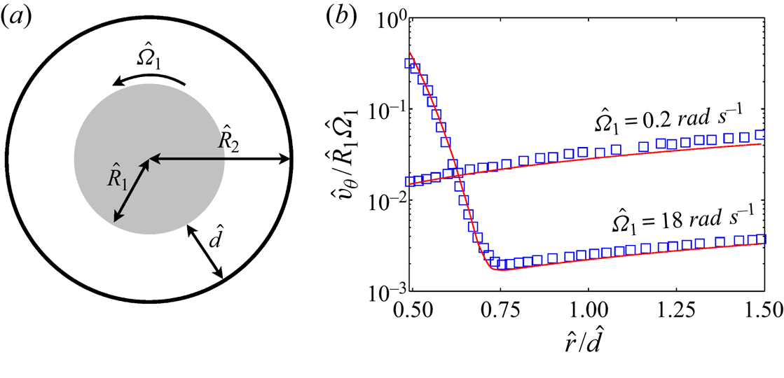
Figure 19. (a) Schematic of the 2-D Couette rheometry between two cylinders of radii  $\hat {R}_1$ (rotating with rotational speed $\hat {\varOmega }_1$) and $\hat {R}_2$ (stationary), (b) red lines are the present computations and the blue symbols are experimental data borrowed form Medina-Bañuelos et al. (Reference Medina-Bañuelos, Marín-Santibáñez, Pérez-González, Malik and Kalyon2017).
The only change that we need to implement in algorithm 1 is step 8,
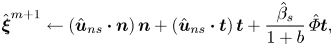 \begin{equation} \hat{\boldsymbol{\xi}}^{m+1} \gets \displaystyle \left( \hat{\boldsymbol{u}}_{{ns}} \boldsymbol{\cdot} \boldsymbol{n} \right) \boldsymbol{n} + \left( \hat{\boldsymbol{u}}_{{ns}} \boldsymbol{\cdot} \boldsymbol{t} \right) \boldsymbol{t} + \frac{\hat{\beta}_s}{1+ b} \,\hat{\varPhi}\boldsymbol{t}, \end{equation}
where  $\hat {\varPhi } = - ( \hat {\boldsymbol {\lambda }}^m \boldsymbol {\cdot } \boldsymbol {t} ) \vert \hat {\boldsymbol {\lambda }}^m \boldsymbol {\cdot } \boldsymbol {t} \vert ^{k-1} + {b}/{\hat {\beta }_s} ( \boldsymbol {\delta } \hat {\boldsymbol {u}}^{m+1} \boldsymbol {\cdot } \boldsymbol {t} - \hat {\boldsymbol {u}}_{ns} \boldsymbol {\cdot } \boldsymbol {t} )$.
As discussed in § 7, although the hydrodynamics features of the flows are different for different  $n$ and $k$, the yield limit of the problems are not dependent on these power indices. We will discuss this in the next few lines by considering a sample example in the circular Couette flow configuration and then will generalize this conclusion.
If the inner cylinder is slippery and the outer cylinder is jagged/treated to eliminate slip, then at the yield limit,
 \begin{equation} B = \frac{\hat{\tau}_y}{\hat{K}} \left( \frac{\hat{d}}{\hat{R}_1 \hat{\varOmega}_1} \right)^n \to \infty\quad \text{or}\quad Y = \frac{\hat{\tau}_y \hat{R}_1^2}{\hat{T}} \to Y_c^-, \end{equation}
the material fully slides over the inner surface and the whole gap is unyielded. Here,  $\hat {T}$ denotes the applied torque on the inner cylinder per unit length. Hence, in the [R] formulation where the scale of the velocity is $\hat {R}_1 \hat {\varOmega }_1$ and $\hat {d}$ is the length scale
 \begin{equation} u_s^* (r=R_1) = 1 = \beta_s \left(\tau_i^* - B_s \right)^k = \beta_s \left(\tau_i^* - \alpha_s B \right)^k \end{equation}
and
 \begin{equation} T^* = 2 {\rm \pi}\left( \sqrt[k]{\frac{1}{\beta_s}} + \alpha_s B \right). \end{equation}
Considering the map between the Bingham and the yield number
 \begin{equation} Y = B \displaystyle \frac{\hat{\mu} \hat{R}_1^3 \hat{\varOmega}_1}{\hat{T} \hat{d}} = \frac{B}{T^*} R_1^2, \end{equation}
we can conclude that the critical yield number is  $Y_c = {R_1^2}/{2 {\rm \pi}\alpha _s}$. Hence, the yield limit is independent of $n$ and $k$. This has been demonstrated in the problems studied in the present study that viscous dissipation is at least one order of magnitude less than the plastic dissipation at the yield limit. Frigaard (Reference Frigaard2019) has shown this before more generally. We have also demonstrated that ‘viscous’ slip dissipation is much less than the ‘plastic’ viscous dissipation at the yield limit for $k=1$. This statement is generally acceptable for $k \neq 1$. Considering that the total slip dissipation term can be split into
 \begin{equation} \int_{\varGamma} \vert \sigma_{nt}^* u_s^* \vert \,\text{d}S = \frac{1}{\beta_s^k} \int_{\varGamma} {u^*_s}^{({1}/{k})+1} \,\text{d}S + B_s \int_{\varGamma} \vert u_s^* \vert \,\text{d}S, \end{equation}
it can be easily understood why the yield limit is independent of  $k$: since the ‘plastic’ slip dissipation term, which is dominant at the yield limit, is independent of $k$. Definition (3.6) is also valid in the case $k \neq 1$ and one can extract the critical ratio of the yield stress to the driving stress by knowing $\hat {\tau }_s$, or alternatively $\alpha _s$ from the slip law.


 Open access