2.1. Resolvent-based estimation

We consider the Navier–Stokes equations

(2.1)\begin{equation} \boldsymbol{\mathsf{M}}\,\partial_t\boldsymbol{q}(\boldsymbol{x},t)=\mathcal{N}(\boldsymbol{q}(\boldsymbol{x},t)), \end{equation}

where $\boldsymbol {q}=[\rho,\,u,\,v,\,w,\,p]^{\text {T}}$ is the state vector, $\mathcal {N}$ denotes the nonlinear Navier–Stokes operator, and the matrix $\boldsymbol{\mathsf{M}}$ is zero for the continuity equation and identity matrix for the rest in incompressible flows, or the identity matrix in compressible flows. Discretisation in space and linearisation around the mean, $\bar {\boldsymbol {q}}(\boldsymbol {x})$, yields

(2.2)\begin{equation} \boldsymbol{\mathsf{M}}\,\partial_t\boldsymbol{q}^{\prime}(\boldsymbol{x},t)-\boldsymbol{\mathsf{A}}(\boldsymbol{x})\,\boldsymbol{q}^{\prime}(\boldsymbol{x},t)=\boldsymbol{f}(\boldsymbol{x},t), \end{equation}

where $\boldsymbol{\mathsf{A}}(\boldsymbol {x})=\partial _q\mathcal {N}|_{\bar {\boldsymbol {q}}}$ is the linear operator obtained from the Jacobian of $\mathcal {N}$, and $\boldsymbol {f}(\boldsymbol {x},t)$ denotes all the remaining nonlinear terms, interpreted as a forcing term in the above equation. The equations are linearised using primitive variables (Karban et al. Reference Karban, Bugeat, Martini, Towne, Cavalieri, Lesshafft, Agarwal, Jordan and Colonius2020). In the resolvent framework, (2.2) is Fourier transformed and rearranged to obtain

(2.3)\begin{equation} \hat{\boldsymbol{q}}(\boldsymbol{x},\omega)=\boldsymbol{\mathsf{R}}(\boldsymbol{x},\omega)\,\hat{\boldsymbol{f}}(\boldsymbol{x},\omega), \end{equation}

where $\boldsymbol {x}=[x,\,y,\,z]^{\text {T}}$ is the space vector, $\omega$ is the angular frequency, the hat indicates a Fourier transformed quantity, and $\boldsymbol{\mathsf{R}}(\boldsymbol {x},\omega )=(-{\rm i}\omega \boldsymbol{\mathsf{M}}-\boldsymbol{\mathsf{A}}(\boldsymbol {x}))^{-1}$ is the resolvent operator. In what follows, notation showing dependence on $\boldsymbol {x}$ and $\omega$ will be dropped for brevity.

The cross-spectral densities of the response and forcing can also be related via the resolvent operator

(2.4)\begin{equation} {\boldsymbol{\mathsf{S}}}=\boldsymbol{\mathsf{R}}{\boldsymbol{\mathsf{P}}}\boldsymbol{\mathsf{R}}^H, \end{equation}

where $\boldsymbol{\mathsf{S}}={\rm E}\{\hat {\boldsymbol {q}}\hat {\boldsymbol {q}}^H\}$ and $\boldsymbol{\mathsf{P}}={\rm E}\{\hat {\boldsymbol {f}}\hat {\boldsymbol {f}}^H\}$ denote the response and forcing cross-spectral density (CSD) matrices, respectively, with ${\rm E}\{\cdot \}$ denoting the expectation operator obtained by averaging different realisations, and the superscript $H$ denoting the conjugate transpose, or Hermitian.

The resolvent operator can be modified in order to explore the relationship between subsets of the forcing and response. For instance, limited measurements at a selection of points, $\boldsymbol {\hat {y}}$, may be considered and related to forcing:

(2.5)$$\begin{gather} \hat{\boldsymbol{y}}=\boldsymbol{\mathsf{C}}\hat{\boldsymbol{q}}, \end{gather}$$

(2.6)$$\begin{gather}\hat{\boldsymbol{y}}=\tilde{\boldsymbol{\mathsf{R}}}\hat{\boldsymbol{f}}, \end{gather}$$

where $\boldsymbol{\mathsf{C}}$ denotes the measurement matrix and $\tilde {\boldsymbol{\mathsf{R}}}\triangleq \boldsymbol{\mathsf{C}}\boldsymbol{\mathsf{R}}$ is the modified resolvent operator that connects forcing to those measurements. We will first investigate the case where $\boldsymbol{\mathsf{C}}=\boldsymbol{\mathsf{I}}$ and $\boldsymbol{\mathsf{R}}$ is full-rank, i.e. $\tilde {\boldsymbol{\mathsf{R}}}$ is also full-rank, before extending our analysis to cases where $\tilde {\boldsymbol{\mathsf{R}}}$ may be singular. Note that (2.2) and (2.3) are exact and provide a bijective relation between the forcing and the response when the resolvent operator is full-rank, and an injective relation when $\boldsymbol{\mathsf{R}}$ is singular.

We employ SPOD to identify coherent structures in the flow. This requires definition of an inner product

(2.7)\begin{equation} \langle \boldsymbol{a},\boldsymbol{b}\rangle = \int_\varOmega \boldsymbol{b}^H{\mathcal{W}}\boldsymbol{a}\,{\rm d}\kern0.7pt\boldsymbol{x}, \end{equation}

where ${\mathcal{W}}$ denotes an energy norm. Equation (2.7) can be written in discrete form as

(2.8)\begin{equation} \langle \boldsymbol{a},\boldsymbol{b}\rangle = \boldsymbol{b}^H\boldsymbol{\mathsf{W}}\boldsymbol{a}, \end{equation}

where $\boldsymbol{\mathsf{W}}$ now accounts for both the energy norm and the numerical quadrature weights. The SPOD modes, which are orthogonal with respect to the inner product defined by (2.8), are obtained by solving the eigenvalue problem

(2.9)\begin{equation} \boldsymbol{\mathsf{S}}\boldsymbol{\mathsf{W}}\boldsymbol{\psi} = \lambda\boldsymbol{\psi}, \end{equation}

where $\boldsymbol {\psi }$ and $\lambda$ denote the eigenvector (SPOD mode) and the eigenvalue (SPOD mode mean square value). The CSD matrix $\boldsymbol{\mathsf{S}}$ can be built from SPOD modes as

(2.10)\begin{equation} \boldsymbol{\mathsf{S}} = \sum_n \lambda_n\boldsymbol{\psi}_n\boldsymbol{\psi}_n^H, \end{equation}

where the subscript $n$ denotes SPOD mode number.

For non-singular $\boldsymbol{\mathsf{R}}$, the forcing mode that generates a given SPOD mode, $\boldsymbol {\psi }$, can be obtained by inverting the resolvent equation

(2.11)\begin{equation} \boldsymbol{\phi}=\boldsymbol{\mathsf{L}}\boldsymbol{\psi}, \end{equation}

where $\boldsymbol{\mathsf{L}}\triangleq (-{\rm i}\omega \boldsymbol{\mathsf{M}}-\boldsymbol{\mathsf{A}})$ and $\boldsymbol{\mathsf{R}}=\boldsymbol{\mathsf{L}}^{-1}$. In the case of $\tilde {\boldsymbol{\mathsf{R}}}$, which is singular, direct inversion is not possible, and the forcing mode associated with the SPOD mode, $\boldsymbol {\psi }$, can then be obtained by means of a pseudo-inverse of $\tilde {\boldsymbol{\mathsf{R}}}$:

(2.12)\begin{equation} \boldsymbol{\phi}=\tilde{\boldsymbol{\mathsf{R}}}^+\boldsymbol{\psi}. \end{equation}

The mode $\boldsymbol {\phi }$ in (2.12) can be understood as the minimal-norm forcing that creates the response, $\boldsymbol {\psi }$, through the resolvent operator, in what is called resolvent-based estimation (RBE) (Martini et al. Reference Martini, Cavalieri, Jordan, Towne and Lesshafft2020; Towne et al. Reference Towne, Lozano-Durán and Yang2020). The forcing structures that are correlated with the response but are ‘silent’, i.e. have no flow response, are not present in the forcing modes estimated using RBE. This might be a desired property for the kinematic modelling of forcing, as whatever is included in the estimated mode is ensured to contribute to the response. However, from a dynamical modelling point of view, elimination of the correlated-but-silent parts of the forcing may hide important dynamic traits of the interaction mechanisms that underpin the forcing structures. Since the silent components are correlated to the observable forces, they are likely generated by the same mechanisms. Thus their study can facilitate identification of these mechanisms. To identify such structures, we consider, in what follows, a data-driven approach that takes into account the forcing and response structures that are actually contained in the data.

2.2. Resolvent-based extended spectral proper orthogonal decomposition

The approach that we present is adapted from the EPOD of Borée (Reference Borée2003), whose goal was to identify correlations between an observed POD mode and some other target field. In Hoarau et al. (Reference Hoarau, Borée, Laumonier and Gervais2006), the method was used in spectral domain. We revisit EPOD also in frequency space, setting the target event as the forcing defined by (2.3). This specific construction of EPOD was first discussed in Towne et al. (Reference Towne, Colonius, Jordan, Cavalieri and Brès2015). We refer here to this implementation as ‘resolvent-based, extended spectral proper orthogonal decomposition’ (RESPOD).

The SPOD modes defined by (2.9) are orthogonal with respect to the norm defined by (2.8), i.e.

(2.13)\begin{equation} \langle \boldsymbol{\psi}_n,\boldsymbol{\psi}_p\rangle = \delta_{np}, \end{equation}

where $\boldsymbol {\psi }_n$ is the $n$th SPOD mode. The SPOD modes provide a complete basis that can be used to expand any realisation of the state vector as

(2.14)\begin{equation} \hat{\boldsymbol{q}} = \sum_n a_n\boldsymbol{\psi}_n, \end{equation}

where the projection coefficient $a_n$ associated with the $n$th eigenmode is obtained by the projection

(2.15)\begin{equation} a_n = \langle \hat{\boldsymbol{q}},\boldsymbol{\psi}_n\rangle. \end{equation}

The orthonormality of the SPOD basis, defined by (2.13), imposes that the projection coefficients satisfy

(2.16)\begin{equation} {\rm E}\{a_n a_p^H\} = \lambda_n\delta_{np}. \end{equation}

This can be seen as follows:

(2.17)\begin{align} {\rm E}\{a_n a_p^H\} &={\rm E}\{\langle\hat{\boldsymbol{q}},\boldsymbol{\psi}_n\rangle\langle\hat{\boldsymbol{q}},\boldsymbol{\psi}_n\rangle^H\} \nonumber\\ &={\rm E}\{\boldsymbol{\psi}_n^H\boldsymbol{\mathsf{W}}\hat{\boldsymbol{q}}\hat{\boldsymbol{q}}^H\boldsymbol{\mathsf{W}}^H\boldsymbol{\psi}_p\}\quad\text{(using (2.8))}\nonumber\\ &=\boldsymbol{\psi}_n^H\boldsymbol{\mathsf{W}}{\rm E}\{\hat{\boldsymbol{q}}\hat{\boldsymbol{q}}^H\}\boldsymbol{\mathsf{W}}^H\boldsymbol{\psi}_p\nonumber\\&= \boldsymbol{\psi}_n^H\boldsymbol{\mathsf{W}}\sum_k\lambda_k\boldsymbol{\psi}_k\boldsymbol{\psi}_k^H\boldsymbol{\mathsf{W}}^H\boldsymbol{\psi}_p\quad\text{(using (2.10))}\nonumber\\ &= \lambda_n\delta_{np}.\end{align}

Here, the expectation operator corresponds to an ensemble average of Fourier realisations. Borée (Reference Borée2003) used (2.14) and (2.16) to show that

(2.18)\begin{align} {\rm E}\{\hat{\boldsymbol{q}}\,a_p^H\}&={\rm E}\left\{\left(\sum_n a_n\boldsymbol{\psi}_n\right)a_p^H\right\}\nonumber\\ &=\sum_n{\rm E}\{a_na_p^H\}\boldsymbol{\psi}_n \nonumber\\ &=\lambda_p\boldsymbol{\psi}_p, \end{align}

which provides an alternative way to compute $\boldsymbol {\psi }_p$ as

(2.19)\begin{equation} \boldsymbol{\psi}_p=\frac{{\rm E}\{\hat{\boldsymbol{q}}\,a_p^H\}}{\lambda_p}, \end{equation}

assuming that $a_p$ is known. Equation (2.19) corresponds to the snapshot approach, shown by Towne et al. (Reference Towne, Schmidt and Colonius2018) to provide a less costly alternative to eigendecomposition of (2.9). Note that for this, one needs to calculate the projection coefficients beforehand. Using the decomposition given in (2.14), we can show that

(2.20)\begin{equation} \langle \hat{\boldsymbol{q}},\hat{\boldsymbol{q}}\rangle = \sum_n a_n a_n^H. \end{equation}

For a given $\hat {\boldsymbol{\mathsf{Q}}}$ defined as the set of realisations of $\hat {\boldsymbol {q}}$, (2.20) can be written as

(2.21)\begin{equation} \langle \hat{\boldsymbol{\mathsf{Q}}},\hat{\boldsymbol{\mathsf{Q}}}\rangle = \sum_n \boldsymbol{a}_n {\boldsymbol{a}_n}^H, \end{equation}

where $\boldsymbol {a}_n\triangleq \langle \hat {\boldsymbol{\mathsf{Q}}},\boldsymbol {\psi }_n\rangle$ denotes the projection coefficient vector. Note that (2.16) holds also for $\boldsymbol {a}_n$, implying the orthogonality of the projection coefficient vectors that correspond to different SPOD modes. Given this orthogonality, rewriting (2.21) by normalising $\boldsymbol {a}_n$ with $\lambda _n^{-1/2}$ as

(2.22)\begin{equation} \langle \hat{\boldsymbol{\mathsf{Q}}},\hat{\boldsymbol{\mathsf{Q}}}\rangle = \sum_n (\boldsymbol{a}_n\lambda_n^{{-}1/2})\lambda_n (\boldsymbol{a}_n^H\lambda_n^{{-}1/2}), \end{equation}

we obtain the eigendecomposition of $\langle \hat {\boldsymbol{\mathsf{Q}}},\hat {\boldsymbol{\mathsf{Q}}}\rangle$. Computing the eigendecomposition given in (2.22), one can obtain the projection coefficients before calculating the SPOD vectors.

Given the forcing vector $\hat {\boldsymbol {f}}$, its RESPOD mode is given by

(2.23)\begin{equation} \boldsymbol{\chi}_p=\frac{{\rm E}\{\hat{\boldsymbol{f}}a_p^H\}}{\lambda_p}. \end{equation}

The RESPOD mode $\boldsymbol {\chi }_p$ provides the forcing mode associated with the $p$th SPOD mode of the response. In Borée (Reference Borée2003), it was shown that the extended modes can be used to isolate, from the target event, the part that is correlated with the observed coherent structure. Given, for instance, the rank-1 representation of $\hat {\boldsymbol {q}}$ as $\hat {\boldsymbol {q}}_1=a_1\boldsymbol {\psi }_1$, the corresponding RESPOD mode $\boldsymbol {\chi }_1$ allows identification of $\hat {\boldsymbol {f}}_1\triangleq a_1\boldsymbol {\chi }_1$, which is the forcing correlated with $\hat {\boldsymbol {q}}_1$. This can be seen by comparing the two cross-covariances between the forcing and the response given as

(2.24)\begin{align} {\rm E}\{\hat{\boldsymbol{f}}\,\hat{\boldsymbol{q}}_1^H\} &= {\rm E}\{\hat{\boldsymbol{f}}a_1^H\boldsymbol{\psi}_1^H\}\nonumber\\ &= {\rm E}\{\hat{\boldsymbol{f}}a_1^H\}\boldsymbol{\psi}_1^H \nonumber\\ &= \lambda_1\boldsymbol{\chi}_1\boldsymbol{\psi}_1^H \end{align}

and

(2.25)\begin{align} {\rm E}\{\hat{\boldsymbol{f}}_1\hat{\boldsymbol{q}}_1^H\} &= {\rm E}\{a_1\boldsymbol{\chi}_1a_1^H\boldsymbol{\psi}_1^H\}\nonumber\\ &= \boldsymbol{\chi}_1{\rm E}\{a_1a_1^H\}\boldsymbol{\psi}_1^H \nonumber\\ &= \lambda_1\boldsymbol{\chi}_1\boldsymbol{\psi}_1^H. \end{align}

This indicates that $\hat {\boldsymbol {f}}_1$ contains all the forcing that is correlated with $\hat {\boldsymbol {q}}_1$.

As the target event we consider here is the forcing term in the resolvent framework, which satisfies (2.6), substituting (2.6) into (2.19), we can show that

(2.26)\begin{align} \boldsymbol{\psi}_p&=\frac{{\rm E}\{\tilde{\boldsymbol{\mathsf{R}}}\hat{\boldsymbol{f}}a_p^H\}}{\lambda_p}\nonumber\\ &=\tilde{\boldsymbol{\mathsf{R}}}\frac{{\rm E}\{\hat{\boldsymbol{f}}a_p^H\}}{\lambda_p} \nonumber\\ &=\tilde{\boldsymbol{\mathsf{R}}}\boldsymbol{\chi}_p, \end{align}

indicating that the correlated response and force modes are dynamically consistent, i.e. they satisfy (2.6).

As mentioned earlier, the relation between forcing and response becomes bijective for a non-singular resolvent operator; i.e. for a given response $\boldsymbol {\psi }$, there is a unique forcing mode that satisfies (2.26) and (2.11). This implies that for the non-singular resolvent operator, the forcing mode identified by RESPOD becomes identical to the RBE mode predicted using (2.11). But for the case of a singular resolvent operator, RESPOD finds both the minimal-norm forcing (also predicted by RBE) necessary to generate the SPOD mode and the correlated-but-silent components of the nonlinear scale interactions.

2.3. Comparison of RBE and RESPOD using a simple model

As a toy model to illustrate the techniques, we consider two rank-3 resolvent operators, $\boldsymbol{\mathsf{R}}_f$ and $\boldsymbol{\mathsf{R}}_s$, that are, respectively, full-rank and singular:

(2.27a,b)\begin{equation} \boldsymbol{\mathsf{R}}_f=\begin{bmatrix} 3 & 0 & 0 \\ 0 & 2 & 0 \\ 0 & 0 & 1 \end{bmatrix},\quad \boldsymbol{\mathsf{R}}_s=\begin{bmatrix} 3 & 0 & 0 & 0 & 0 \\ 0 & 2 & 0 & 0 & 0 \\ 0 & 0 & 1 & 0 & 0 \end{bmatrix}. \end{equation}

Both systems are driven by random forcing vectors, $\hat {\boldsymbol {f}}_f=[c_1,\,c_2,\,c_3]^{\text {T}}$ and $\hat {\boldsymbol {f}}_s=[c_1,\,c_2,\,c_3,\,3c_1,\,c_4]^{\text {T}}$, respectively, where $c_i$ is a random number with zero mean and unit variance. The random forcing realisations are generated using Matlab random number generator. The random number seeding is re-initialised for each simulation to ensure using the same random value series, which makes the results repeatable. The fourth and fifth components in $\hat {\boldsymbol {f}}_s$ project onto the null space of $\boldsymbol{\mathsf{R}}_s$, but the fourth component is fully correlated to the first since both contain the same random variable, $c_1$. Re-initialisation of the random number generator ensures that the first three components of $\hat {\boldsymbol {f}}_f$ and $\hat {\boldsymbol {f}}_s$, those that are observable through the corresponding resolvent operators, are identical. The responses obtained for the two systems are thereby identical. Two tests are carried out using 10 and 500 realisations, respectively. The leading SPOD mode for both singular and non-singular systems is obtained as $\boldsymbol {\psi }= [-0.9622, \, 0.2576, \, -0.0890]^{\text {T}}$ when 10 realisations are considered, and $\boldsymbol {\psi }= [-0.9943, \, -0.1056, \, 0.0148]^{\text {T}}$ with 500 realisations. As the forcing in the full-rank model problem is white, i.e. $\boldsymbol{\mathsf{P}}=\boldsymbol{\mathsf{I}}$, by inspection, one can see that the expected value for the leading SPOD mode is $\boldsymbol {\psi }=[1,\,0,\,0]^{\text {T}}$ (or its negative). The predictions based on realisations converge to the expected value with an algebraic convergence.

Using 10 realisations, the forcing modes computed using RBE and RESPOD, respectively $\boldsymbol {\phi }_{f/s}$ and $\boldsymbol {\chi }_{f/s}$, are, for the full-rank system,

(2.28a,b)\begin{equation} \boldsymbol{\phi}_f=\begin{bmatrix} -0.3207 \\ 0.1288 \\ -0.0890 \end{bmatrix}\quad \text{and}\quad \boldsymbol{\chi}_f=\begin{bmatrix} -0.3207 \\ 0.1288 \\ -0.0890 \end{bmatrix}, \end{equation}

while for the singular system we obtain

(2.29a,b)\begin{equation} \boldsymbol{\phi}_s=\begin{bmatrix} -0.3207 \\ 0.1288 \\ -0.0890 \\ 0 \\ 0 \end{bmatrix}\quad \text{and}\quad \boldsymbol{\chi}_s=\begin{bmatrix} -0.3207 \\ 0.1288 \\ -0.0890 \\ -0.9622 \\ 0.0283 \end{bmatrix}. \end{equation}

The same results for the cases based on 500 realisations are given as

(2.30a–d)\begin{align} \boldsymbol{\phi}_f=\begin{bmatrix} -0.3314 \\ -0.0528 \\ 0.0148 \end{bmatrix}, \quad \boldsymbol{\chi}_f=\begin{bmatrix} -0.3314 \\ -0.0528 \\ 0.0148 \end{bmatrix}, \quad \boldsymbol{\phi}_s=\begin{bmatrix} -0.3314 \\ -0.0528 \\ 0.0148 \\ 0 \\ 0 \end{bmatrix}\quad \text{and}\quad \boldsymbol{\chi}_s=\begin{bmatrix} -0.3314 \\ -0.0528 \\ 0.0148 \\ -0.9943 \\ 0.0066 \end{bmatrix}. \end{align}

As expected, the results obtained using RBE and RESPOD are identical in the full-rank system. The fourth component of $\boldsymbol {\chi }_s$ is three times the first component, where this correlation information was included in the definition of $\hat {\boldsymbol {f}}_s$. Although the RBE method, which finds the minimal-norm forcing for a given response, and the RESPOD method, which finds the correlated forcing for a given response, ask different questions, their results are the same when the resolvent operator is full-rank. This is because for a full-rank resolvent operator, no silent forcing exists. When different numbers of realisations are considered, RBE and RESPOD yield identical results when the resolvent operator is full-rank; this is because the SPOD response mode and the RESPOD forcing mode have identical convergence in that case. This will be the case when the two methods are based on the exact same realisations, and the realisations are consistent, i.e. they satisfy (2.6). The results may differ if the database contains noise on the response and/or the forcing, which is outside the scope of this study.

For the singular case, the forcing predictions obtained using RBE and RESPOD differ in the silent forcing components. RBE, by construction, predicts zero forcing in these components, while RESPOD captures the correlated information between the first and fourth components, and the fifth component, which is uncorrelated with the response, tends to zero. In a more complicated system, involving turbulent flow for example, this additional information obtained from RESPOD may be expected to provide additional insight regarding the mechanisms that underpin the forcing.

Note that although the SPOD modes are unit vectors in the Euclidean norm, the associated forcing modes obtained using RESPOD or RBE are not unit vectors. In (2.23), we see that the RESPOD mode is normalised using the response eigenvalue, so a unit norm is not ensured. Similarly, (2.11) implies that for a unit SPOD vector, the associated forcing mode obtained using RBE is not necessarily a unit vector. The norm of the forcing mode obtained by RBE/RESPOD is related by the associated gain. In RBE, amplified forcing modes will have a smaller-than-unity norm, such that $\boldsymbol{\mathsf{R}}\boldsymbol {\phi }$ will be unity. In RESPOD, besides the associated gain, the norm also depends on the correlated-but-silent parts.

3.1. Database and definitions

The flow data are provided by DNS of the incompressible Navier–Stokes equations using the ‘ChannelFlow’ code (see www.channelflow.ch for details). The DNS details are provided in table 1, where $T_{max}$ and $\Delta t$ denote the total simulation time and the time step, respectively, and $L_{x/y/z}$ and $N_{x/y/z}$ denote the domain and the grid size, respectively; the superscript $+$ denotes a near-wall unit. For dealiasing, a larger number of Fourier modes ($3/2$ times $N_x$ and $N_z$) was used in the simulations. The subscripts $x$, $y$ and $z$ denote the streamwise, wall-normal and spanwise directions, respectively. The mean velocities and the root-mean-square values of the DNS data used were compared against the literature (del Álamo & Jiménez Reference del Álamo and Jiménez2003) in Morra et al. (Reference Morra, Nogueira, Cavalieri and Henningson2021), and are therefore not presented here. To show the statistical convergence of the simulation, we check the balance in the mean momentum equation given as

(3.1)\begin{equation} 0 = \frac{1}{Re_\tau} + \frac{{\rm d}^2U_x^+}{{\rm d}{y^{+}}^2}-\frac{\overline{uv}^+}{{{\rm d} y}^+}, \end{equation}

where $U_x$ denotes the mean streamwise velocity, $u$ and $v$ denote the velocity fluctuations in the streamwise and wall-normal directions, respectively, an overbar indicates temporal averaging, and the superscript $+$ denotes quantities in wall units (see Wei et al. (Reference Wei, Fife, Klewicki and McMurtry2005) for further details). Integrating (3.1) in $y^+$ yields

(3.2)\begin{equation} -y = \frac{{\rm d}U_x^+}{{\rm d}{y^{+}}}-\overline{uv}^+. \end{equation}

The terms in (3.2) are plotted in figure 1, where it is seen that the summation of ${{\rm d}U_x^+}/{{\rm d}{y^{+}}}$ and $-\overline {uv}^+$ satisfies (3.2), hence the momentum balance is reached.

Figure 1. Momentum budget plot for the DNS of the channel flow.

Table 1. Details of the DNS database.

The Fourier realisations are calculated using 128 fast Fourier transform (FFT) points with 80 % overlap between successive time blocks. The second-order exponential windowing function given in Martini et al. (Reference Martini, Cavalieri, Jordan and Lesshafft2019) is used to perform the Fourier transform. The forcing correction associated with the windowing function is added to the Fourier realisations of the forcing as described in Martini et al. (Reference Martini, Cavalieri, Jordan and Lesshafft2019) to ensure that the forcing and the response are related accurately to each other via the resolvent operator, as shown by Morra et al. (Reference Morra, Nogueira, Cavalieri and Henningson2021) and Nogueira et al. (Reference Nogueira, Morra, Martini, Cavalieri and Henningson2021).

The resolvent framework for incompressible isothermal viscous flows is given as follows. Defining $\boldsymbol {u}_{tot}=\boldsymbol {U}+\boldsymbol {u}$ and $p_{tot}=P+p$ – where $\boldsymbol {U}=[U_x,\, 0,\, 0]^{\rm T}$ and $\boldsymbol {u}=[u,\, v,\, w]^{\rm T}$ are the mean and fluctuation velocities, respectively, defined in Cartesian coordinates ordered in streamwise, wall-normal and spanwise directions, and $P$ and $p$ are the mean and fluctuating pressure – the governing equations for momentum fluctuations are given as

(3.3)\begin{equation} \left. \begin{gathered} \partial_t\boldsymbol{u}+(\boldsymbol{U}\boldsymbol{\cdot}\boldsymbol{\nabla})\boldsymbol{u} +(\boldsymbol{u}\boldsymbol{\cdot}\boldsymbol{\nabla})\boldsymbol{U}={-}\boldsymbol{\nabla} p + \frac{1}{Re}\nabla^2\boldsymbol{u}+\boldsymbol{b}+\boldsymbol{f},\\ \boldsymbol{\nabla}\boldsymbol{\cdot}\boldsymbol{u}=0, \end{gathered} \right\} \end{equation}

where $Re=U_{bulk}h/\nu$ denotes the Reynolds number, $\nu$ is the molecular viscosity, $\boldsymbol {f}=-(\boldsymbol {u}\boldsymbol {\cdot }\boldsymbol {\nabla })\boldsymbol {u}$ and $\boldsymbol {b}=-\boldsymbol {\nabla } P + Re^{-1}\nabla ^2\boldsymbol {U}-(\boldsymbol {U}\boldsymbol {\cdot }\boldsymbol {\nabla })\boldsymbol {U}$. Spatial derivative operators are given as $\boldsymbol {\nabla }=[\partial _x,\, \partial _y,\, \partial _z]^\textrm {T}$ and $\nabla ^2=\boldsymbol {\nabla }\boldsymbol {\cdot }\boldsymbol {\nabla }$. Defining the state vector $\boldsymbol {q}=[u,\,v,\,w,\,p]^\textrm {T}$, and taking the Fourier transform in all homogeneous dimensions ($x$, $z$ and $t$) with the ansatz $\hat {\boldsymbol {q}}(\alpha,y,\beta,\omega ) \exp ({\textrm {i}(\alpha x + \beta z - \omega t)})$, the governing equations given in (3.3) can be written in matrix form as

(3.4)\begin{equation} {\rm i}\omega\boldsymbol{\mathsf{M}}\hat{\boldsymbol{q}}-{\boldsymbol{\mathsf{A}}}\hat{\boldsymbol{q}}=\boldsymbol{B}\hat{\boldsymbol{f}}, \end{equation}

considering that $\omega$, $\alpha$ and $\beta$ are not simultaneously zero, such that the $\boldsymbol {b}$ term, which varies only in $y$, has no contribution. Note that taking the Fourier transform in $x$ and $z$ allows an accurate and inexpensive explicit construction of the resolvent operator using pseudo-spectral methods.

Defining the transformation matrix $\hat {\boldsymbol {u}}=\boldsymbol{\mathsf{C}}\hat {\boldsymbol {q}}$, we can write (3.4) in resolvent form as

(3.5)\begin{equation} \hat{\boldsymbol{u}}=\boldsymbol{\mathsf{R}}\hat{\boldsymbol{f}}, \end{equation}

where $\boldsymbol{\mathsf{R}}=\boldsymbol{\mathsf{C}}(-\textrm {i}\omega \boldsymbol{\mathsf{M}}-\boldsymbol{\mathsf{A}})^{-1}\boldsymbol {B}$, and a hat denotes a Fourier-transformed variable. The matrices $\boldsymbol{\mathsf{A}}$, $\boldsymbol {B}$, $\boldsymbol{\mathsf{C}}$ and $\boldsymbol{\mathsf{M}}$ are given in explicit form in Appendix A.

To investigate the wall-attached structures, we will define a measurement matrix

(3.6)\begin{equation} \tilde{\boldsymbol{\mathsf{C}}}=[0\; 0\; \partial_z|_{y=0}\; 0], \end{equation}

which yields, when we left-multiply it with (3.5),

(3.7)\begin{equation} \tau_z=\tilde{\boldsymbol{\mathsf{C}}}\boldsymbol{\mathsf{R}}\hat{\boldsymbol{f}}, \end{equation}

where $\tau _z=\partial _zw|_{y=0}$ is the spanwise wall shear. We choose to measure $\tau _z$ considering that it is strongly associated to quasi-streamwise vortices. We then apply the RESPOD to obtain the forcing that is correlated with the wall shear. Note that since $\tau _z$ is a scalar quantity, it has one SPOD mode that is also scalar, and the associated forcing is bound to be rank-1, which yields

(3.8)\begin{equation} \psi=\tilde{\boldsymbol{\mathsf{C}}}\boldsymbol{\mathsf{R}}\boldsymbol{\chi}. \end{equation}

The RESPOD mode $\boldsymbol {\chi }$, when multiplied with the resolvent operator $\boldsymbol{\mathsf{R}}$, yields the velocity field that is correlated with $\tau _z$. The proof is provided in the following. Using the velocity vector $\hat {\boldsymbol {u}}$ as the target event in (2.23) instead of the forcing $\hat {\boldsymbol {f}}$, one can obtain the velocity field $\boldsymbol {\xi }$ that is correlated with $\tau _z$ as

(3.9)\begin{equation} \boldsymbol{\xi}=\frac{{\rm E}\{\hat{\boldsymbol{u}}a^H\}}{\lambda}, \end{equation}

where, for the particular case of $\tau _z$ being a scalar, $a=\langle \tau _z,1\rangle$ and the eigenvalue $\lambda$ is obtained simply by ${\rm E}\{\tau _z\tau _z^H\}$. Substituting (3.5) into (3.9) gives

(3.10)\begin{equation} \boldsymbol{\xi}=\boldsymbol{\mathsf{R}}\boldsymbol{\chi}, \end{equation}

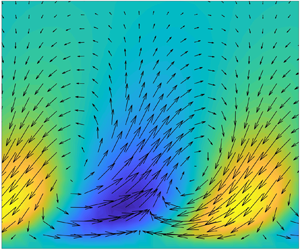
which proves the above statement. Since $\boldsymbol {\xi }$, also rank-1, corresponds to all and the only parts in $\hat {\boldsymbol {u}}$ that are correlated with $\tau _z$ (see the discussion in § 2.2 or alternatively Borée (Reference Borée2003)), we consider it as the wall-attached part of $\hat {\boldsymbol {u}}$.

3.2. Power spectral densities

The DNS database is decomposed into Fourier modes in streamwise and spanwise directions. In figure 2, we show the power spectral density (PSD) of $\tau _z$ at different $\alpha ^+$ and $\beta ^+$ values. Peak energy location is seen to move towards higher $\omega$ and $\beta$ for increasing $\alpha$ while the amplitude reduces. Attached eddies are expected to be the main energy-containing structures in the flow (Townsend Reference Townsend1976) and exhibit a self-similar organisation. Self-similarity implies that structures in the same hierarchy should have constant streamwise-to-spanwise and streamwise-to-wall-normal ratios. In a flow database that is decomposed into Fourier modes in the streamwise and spanwise directions, self-similarity can be investigated by imposing it in the horizontal plane by fixing the streamwise-to-spanwise aspect ratio (AR) and searching for it in the wall-normal direction, similar to Hellström et al. (Reference Hellström, Marusic and Smits2016) and Hellström & Smits (Reference Hellström and Smits2017). In what follows, we first set $\rm\lambda _x^+/\rm\lambda _z^+=6$, where $\rm\lambda _x$ and $\rm\lambda _z$ are the streamwise and spanwise wavelengths, and look for self-similar structures at this AR. We then extend our analysis to a range of ARs and provide an overall view of self-similarity for the given channel flow. We first investigate self-similarity of structures at frequencies with high spectral energy, which is followed by investigation of self-similarity in less energetic structures.

Figure 2. PSD map of $\tau _z$ for different $\alpha ^+$ values.

Maximum-energy-containing frequency $\omega _{max}$ for different $\alpha ^+$ values with $\textrm {AR}=6$ is shown in figure 3. We see that $\omega _{max}$ increases almost linearly with $\alpha ^+$. We approximate this trend with the red line shown in the figure, which is the best linear fit minimising $L_1$-norm error. The $L_1$-norm is chosen for the trend line to be less sensitive to outliers. The frequency corresponding to each $(\rm\lambda _x^+,\rm\lambda _z^+)$ pair is selected using this trend line.

Figure 3. Maximum-energy-containing frequency, $\omega _{max}$, of spanwise wall shear $\tau _z$ for different Fourier-mode pairs with $\textrm {AR}=6$. The red dashed line indicates the best fit minimising $L_1$-norm error.

The accuracy of the forcing database in $Re_\tau =543$ flow is verified by comparing the state $\hat {\boldsymbol {q}}$ to its resolvent-based prediction $\boldsymbol{\mathsf{R}}\hat {\boldsymbol {f}}$ in figure 4. Such an evaluation has already been performed by Morra et al. (Reference Morra, Nogueira, Cavalieri and Henningson2021) for two dominant structures, and it is here extended to a broader range of wavenumbers. As seen in the figure, the resolvent-based prediction of the response matches the DNS state data for the entire wavenumber span considered.

Figure 4. PSD of the response $\hat {\boldsymbol {q}}$ (solid lines) in comparison to its resolvent-based prediction $\boldsymbol{\mathsf{R}}\hat {\boldsymbol {f}}$ (markers) at $\omega _{max}$ for different Fourier-mode pairs with $\textrm {AR}=6$. Wavelengths plotted are $\rm\lambda _x^+=487$, 569, 683, 853, 1137 and 1706.

The square root of PSD of the wall shear $\tau _z$ calculated at $\omega _{max}$ is shown in figure 5. The amplitude is seen to decrease for increasing $\alpha ^+$ as expected from figure 2. The trend is almost linear for $\alpha ^+>7.4\times 10^{-3}$.

Figure 5. Amplitude spectral density of spanwise wall shear $\tau _z$ at $\omega _{max}$ for different Fourier-mode pairs with $\textrm {AR}=6$.

3.3. Wall-attached coherent structures and associated forcing for $\textrm {AR}=6$

We now focus on the wall-attached structures at the peak-energy frequency, $\omega _{max}^+$, for each $(\rm\lambda _x^+,\rm\lambda _z^+)$ pair with AR fixed at 6. The modes are forced to be symmetric in $u$ and $w$ (and anti-symmetric in $v$) about the channel centre in the wall-normal direction by averaging the flow fields in the bottom and the upper halves of the channel (considering a minus sign in $v$), as in Abreu et al. (Reference Abreu, Cavalieri, Schlatter, Vinuesa and Henningson2020a). In figure 6, wall-shear-associated forcing modes obtained using RESPOD and RBE methods, respectively, and the velocity fields generated by these forcing modes, are shown. Note that the mode amplitudes are adjusted to have unit wall shear. The forcing from the RBE method, $\boldsymbol {\phi }$, shows that the spanwise and wall-normal components of forcing drive the wall-shear dynamics observed in the flow at this AR, while the streamwise component is almost not required. For the forcing from the RESPOD method, $\boldsymbol {\chi }$, on the other hand, the forcing mechanisms that generate wall shear involve to a large extent the streamwise component of forcing, although its overall contribution to wall-shear dynamics can be small, as suggested by the RBE results. This indicates strong cancellations among the responses to different forcing components, similar to the results in Morra et al. (Reference Morra, Nogueira, Cavalieri and Henningson2021). This will be investigated further at the end of this subsection. As discussed earlier, the response $\boldsymbol {\xi }=\boldsymbol{\mathsf{R}}\boldsymbol {\chi }$ yields the velocity field associated with the wall shear. Similarly, $\boldsymbol{\mathsf{R}}\boldsymbol {\phi }$ can be interpreted as best prediction of the correlated velocity field when no data for forcing are available. This amounts to flow estimation using low-rank measurements with the assumption of forcing CSD $\boldsymbol{\mathsf{P}}=\boldsymbol{\mathsf{I}}$, as discussed in Martini et al. (Reference Martini, Cavalieri, Jordan, Towne and Lesshafft2020). We see that the velocity modes associated with the wall shear are significantly overpredicted when RBE is used.

Figure 6. Comparison of the wall-shear-associated forcing modes obtained by RESPOD (a,e,i) and RBE (b, f,j), and the corresponding velocity fields ((c,g,k) and (d,h,l), respectively), at $\rm\lambda _x^+=341$, 487, 682, 1137 and 1706, with $\rm\lambda _x^+/\rm\lambda _z^+=6$.

As mentioned above, the difference between the minimal-norm forcing $\boldsymbol {\phi }$ and the wall-shear-correlated forcing $\boldsymbol {\chi }$ implies that contributions to $\tau _z$ from each component of $\boldsymbol{\mathsf{P}}_{\chi }=\boldsymbol {\chi }\boldsymbol {\chi }^H$ cancel each other to a significant extent. To understand the effect of a particular component of $\boldsymbol {\chi }$ (or $\boldsymbol {\phi }$), we calculate the wall shear using $\boldsymbol {\chi }$ (or $\boldsymbol {\phi }$) with that component masked. The resulting wall-shear PSDs for partially masked $\boldsymbol {\chi }$ and $\boldsymbol {\phi }$, respectively, are shown in figure 7. The forcing modes are scaled such that using the full forcing mode generates a wall shear with unit amplitude at each wavenumber pair. For the wall-shear-correlated forcing $\boldsymbol {\chi }$, we see that the wall-normal component has the least effect on the resulting $\tau _z$ amplitude at every wavenumber pair. In the case of minimal-norm forcing $\boldsymbol {\phi }$, on the other hand, the streamwise component has negligible effect on wall-shear dynamics. This implies that the mechanisms involved in the two forcing modes are indeed different, although amounting to the same overall response. For $\boldsymbol {\phi }$, wall shear is generated by a pure streamwise vortical forcing at every wavenumber. For $\boldsymbol {\chi }$, it is the streamwise and spanwise components that are important, with the latter being the main driving component. This implies that turbulence does not follow the optimal path to generate wall-shear fluctuations. The fact that masking $\chi _x$ increases $\sqrt {{\rm E}\{\tau _z\tau _z^*\}}$ implies that simultaneous presence of the streamwise and spanwise components causes some cancellation in the wall-shear fluctuation amplitude.

Figure 7. Square root of PSD of $\tau _z$ obtained using partially masked $\boldsymbol {\chi }$ (a) and $\boldsymbol {\phi }$ (b) at different wavenumbers, with $\textrm {AR}=6$. Unmasked PSDs are all unity, shown by the dashed lines.

Note that the predictions from the RBE method can be improved using an eddy-viscosity model. The eddy viscosity is often used to enhance modelling properties of the resolvent operator (Morra et al. Reference Morra, Semeraro, Henningson and Cossu2019; Pickering et al. Reference Pickering, Rigas, Sipp, Schmidt and Colonius2019). It was used in Towne et al. (Reference Towne, Lozano-Durán and Yang2020) and was more effective to recover flow ($\boldsymbol {q}$) statistics. As shown in Morra et al. (Reference Morra, Nogueira, Cavalieri and Henningson2021), the eddy viscosity embeds some of the forcing statistics in the resolvent operator, but not all (Amaral et al. Reference Amaral, Cavalieri, Martini, Jordan and Towne2021). A drawback of using eddy viscosity is that the forcing of an eddy-viscosity-based resolvent operator does not correspond to the actual nonlinear Navier–Stokes terms. Since we are interested in these nonlinear terms, we use the molecular-viscosity-based resolvent operator, as it allows us to probe directly the nonlinear terms via the forcing $\boldsymbol {f}$.

3.4. Self-similarity of wall-attached forcing and response structures for $AR=6$

Townsend's AEH states that the attached eddies scale in size with respect to their distance to the wall (Townsend Reference Townsend1976; Perry & Chong Reference Perry and Chong1982). We will assess the validity of this assumption for the wall-attached structures investigated in this study. As mentioned earlier, by keeping the AR fixed, we impose self-similarity in the streamwise and spanwise directions. Regarding the modes seen in figure 6, although the amplitudes show different trends, particularly for different forcing components, we see that the mode shapes exhibit to a certain extent a self-similar trend, except for the wall-normal component of the forcing mode $\boldsymbol {\chi }$. The self-similarity can be made apparent by a proper scaling of the modes in the wall-normal direction and normalisation of each mode with its peak amplitude. To assess the self-similarity in the wall-normal direction, Hellström et al. (Reference Hellström, Marusic and Smits2016) proposed a scaling based on the peak of the POD modes. In a similar spirit, we propose a scaling based on the integral function

(3.11)\begin{equation} g(\alpha,y) = \int_0^{y} |{\xi}_x(\alpha,y,\beta(\alpha),\omega_{max}(\alpha))|\,{{\rm d} y}, \end{equation}

where ${\xi }_x$ is the streamwise component of the wall-shear-correlated velocity mode $\boldsymbol {\xi }$, and we use this function to define a characteristic length scale $y_h$ such that $g(\alpha,y_h)=g(\alpha,H)/2$, where $H$ is the channel half-height. In other words, $y_h(\alpha )$ is the wall-normal position that divides the area under $|\xi _x|$ into two equal parts. The $\beta ^+$ dependence of $y_h^+$ is shown in figure 8. We repeat this analysis with ${\chi }_z$ instead of ${\xi }_x$ and show the results in the same figure. The component $\chi _z$ is chosen as it is the dominant component in generating wall shear, as shown in figure 7. Consistent with the attached-eddy hypothesis (Townsend Reference Townsend1976; Perry & Chong Reference Perry and Chong1982), the wall-attached structures with the same AR computed at the peak-energy frequency, $\omega _{max}$, follow a $\beta ^{-1}$ trend except for the very small scales ($\beta ^+>0.09$). The forcing modes also follow a similar trend, which again deviates from $\beta ^{-1}$ at small scales. The wall-attached structures scaling with $\beta ^{-1}$, consistent with the AEH, suggests a self-similar behaviour. The forcing modes following a similar trend suggests that the mechanisms that generate these structures may also be self-similar, i.e. dynamic self-similarity in addition to Townsend's kinematic self-similarity.

Figure 8. Mode centre $y_h^+$ obtained using $\xi _x$ (square) and $\chi _z$ (triangle) at different wavenumbers, with $\textrm {AR}=6$. The dashed line shows the $1/{\beta ^+}$ trend.

The characteristic eddy length scale, $y_h$, can now be used to normalise the structures seen in figure 6. We reconstruct the forcing and response modes in the $y$–$z$ plane, which corresponds to channel cross-section. Mode phases at each $(\rm\lambda _x^+,\rm\lambda _z^+)$ pair are shifted to have $\angle \tau _z=0$. We use $y_h$ based on ${\xi }_x$ to scale both the forcing and response modes in the $y$- and $z$-directions. We normalise the wall-normal and spanwise components of both forcing modes, $\boldsymbol {\chi }$ and $\boldsymbol {\phi }$, with ${\chi }_x$, and similarly those of the response modes with ${\xi }_x$. The reconstructed modes, shown in figure 9, reveal self-similarity of the wall-attached structures and the associated forcing. The streaks and the streamwise vortices seen in the response modes $\boldsymbol {\xi }$ indicate that the wall shear $\tau _z$ is associated with the lift-up mechanism (Brandt Reference Brandt2014). As discussed earlier, the RBE method overpredicts the wall-shear-correlated velocity field. The modes are once again reminiscent of the lift-up mechanism, with the streaks and the streamwise vortices considerably more tilted in the spanwise direction. The optimal forcing $\boldsymbol {\phi }$, which is sufficient to create the wall shear observed in the flow, has a streamwise-vortex-like structure. This is consistent with the optimal forcing modes in Couette flow discussed in Hwang & Cossu (Reference Hwang and Cossu2010a). The forcing modes that actually take place in the flow, on the other hand, do not reveal immediately such a simple structure, although showing self-similarity in itself.

Figure 9. Reconstruction of wall-shear-associated forcing modes $\boldsymbol {\chi }$ (a,e,i) and $\boldsymbol {\phi }$ (b, f,j), and the corresponding velocity fields ((c,g,k) and (d,h,l), respectively) in the $y$–$z$ plane at three wavenumbers (from top to bottom). Colour plots indicate the $x$-component, while vectors show $y$- and $z$-components. The domain is rescaled using $y_h$ for each wavenumber.

3.5. Extension of self-similarity analysis to other ARs

Given the self-similarity observed at the wall-attached structures with $\textrm {AR}=6$, we now extend our analysis to other ARs ranging from 2 to 10. Once again we look for the dominant structures extracted by choosing the maximum-energy-containing frequency for each $(\rm\lambda _x^+,\rm\lambda _z^+)$ pair for a given AR. Figure 10 shows the peak-energy frequency $\omega _{max}^+$ versus wavenumber plots for different ARs, together with the linear trends minimising $L_1$-norm error. We see that all the trends for different ARs collapse onto the same line, given by $\omega ^+=9.04\alpha ^+ + 0.0166$. We use this linear trend to set the frequency for a given $(\rm\lambda _x^+,\rm\lambda _z^+)$ pair at a given AR.

Figure 10. Peak-energy-containing frequencies for different wavenumber pairs with fixed AR. Different markers indicate different AR values. The coloured dashed lines correspond to the best-fit lines for different ARs, using the same colour code.

We calculate the mode centre $y_h$ and investigate its change with respect to the spanwise wavenumber $\beta$. Similar to the analysis conducted for the $\textrm {AR}=6$ case, we compute $y_h$ using ${\xi }_x$ and ${\chi }_z$, respectively, and show the results for different ARs in figure 11. Overall, we observe the $\beta ^{-1}$ trend for both the response and forcing structures at every AR, which imply that self-similarity may be present for all the dominant wall-attached structures and the associated forcing for a broad range of ARs. In general, the small-scale structures near the wall are seen to deviate from the $\beta ^{-1}$ trend for all the ARs. This deviation may be due to increasing viscous effects at this region. We see that at certain ARs, the largest forcing and/or response structures also deviate from the $\beta ^{-1}$ trend. This may be caused by these structures being affected by the other half-channel at the given $Re$.

Figure 11. Mode centre $y_h^+$ obtained using $\xi _x$ (square) and and $\chi _z$ (triangle) at different wavenumbers. Each subplot shows results for a different AR. The dashed lines show the $1/{\beta ^+}$ trends.

To quantify self-similarity, we define the following measure. Given $\zeta$ as any component of any response or forcing mode for a given $(\rm\lambda _x^+,\rm\lambda _z^+)$ pair at a given AR, we first normalise $\zeta$ with its peak value, given as $\zeta _n$, and then perform $y_h$ scaling as

(3.12)\begin{equation} \zeta_n(y)=\tilde{\zeta}_n(y/y_h), \end{equation}

to get $\zeta _n$ in self-similar coordinates, where $y_h$ is calculated using ${\xi }_x$. After performing this analysis for all the wavenumber pairs at a given AR, we find the ‘mean’ self-similar mode by averaging these modes as

(3.13)\begin{equation} {\rm E}\{\tilde{\zeta}_n\}=\frac{1}{N}\sum_i^N\tilde{\zeta}_n^{(i)}, \end{equation}

where $N$ denotes the total number of wavenumber pairs at that AR. We then compute the alignment of $\tilde {\zeta }_n^{(i)}$, which corresponds to the $i{\textrm {th}}$ wavenumber pair, with this mean self-similar mode as

(3.14)\begin{equation} \gamma_\zeta^{(i)}=\frac{|\langle\tilde{\zeta}_n^{(i)},{\rm E}\{\tilde{\zeta}_n\}\rangle|}{\sqrt{\langle\tilde{\zeta}_n^{(i)},\tilde{\zeta}_n^{(i)}\rangle}\sqrt{\langle {\rm E}\{\tilde{\zeta}_n\},{\rm E}\{\tilde{\zeta}_n\}\rangle}}. \end{equation}

According to (3.14), $\gamma _\zeta ^{(i)}$ becomes 1 in case of perfect self-similarity, and 0 in case of no self-similarity. Assuming that a self-similar behaviour is present in all the data considered, the averaging process will clearly reveal the self-similar profile, with each data point showing small deviations from it. Note, however, that if self-similar behaviour is found in only a limited range of parameters, e.g. $\rm\lambda _z$, then including data points outside this range can mask the self-similar behaviour. That is, the approach used is prone to false negatives, being a conservative identification method.

In figure 12, we show the similarity maps $\gamma _{\boldsymbol {\chi }}$, $\gamma _{\boldsymbol {\phi }}$ and $\gamma _{\boldsymbol {\xi }}$ for different ARs and $\alpha ^+$ values. White regions in the figure correspond to wavenumber pairs that are not contained in the database. In general, as all the modes have similar phase and the mode shapes are never too different from each other, for almost all the cases the self-similarity coefficient given in (3.14) takes values close to 1. However, we observed by visual inspection that self-similarity is sufficiently clear only for $\gamma >0.9$. Therefore, we set this as the lower limit in the maps shown in figure 12. The wall-attached structures given by $\boldsymbol {\xi }$ show strong self-similarity except the very-large-scale structures, which, once again, potentially are affected by the other half-channel. We see a slight reduction in the self-similarity of the smallest scales, particularly in the wall-normal and spanwise velocity components, $\xi _y$ and $\xi _z$, respectively. This reduced self-similarity is in agreement with the deviation of the small-scale structures from the $\beta ^{-1}$ trend as shown in figure 11.

Figure 12. Self-similarity maps $\gamma _{\boldsymbol {\chi }}$ (a,d,g), $\gamma _{\boldsymbol {\phi }}$ (b,e,h) and $\gamma _{\boldsymbol {\xi }}$ (c, f,i), for different ARs and $\alpha ^+$ values. Panels (a–c), (d–f) and (g–i) correspond to the $x$-, $y$- and $z$-components, respectively.

Parallel to the wall-attached structures, the associated minimal-norm forcing, $\boldsymbol {\phi }$ shows also self-similarity, although slightly reduced, in all its components except the large-scale structures. Note that the minimal-norm forcing $\boldsymbol {\phi }$ involves only the response and the resolvent operator. Given that the response is self-similar, this result implies that the resolvent operator induces self-similarity as well. This is in line with the findings of Hwang & Cossu (Reference Hwang and Cossu2010a), McKeon (Reference McKeon2017) and Sharma et al. (Reference Sharma, Moarref and McKeon2017).

Regarding the wall-shear-correlated forcing $\boldsymbol {\chi }$, we observe self-similarity in the streamwise and spanwise components, $\chi _x$ and $\chi _z$, respectively, with that in $\chi _z$ being slightly higher. No such self-similarity is seen in the wall-normal component $\chi _y$. A potential reason for that may be the lower amplitude of forcing modes in the $y$-direction compared to other components, as illustrated in figure 6; statistical convergence for low-amplitude components is sufficiently harder, as $\chi _y$ is the smallest and the least effective forcing component in terms of wall-shear dynamics (see figure 7). Even being limited to $\chi _x$ and $\chi _z$, given that wall shear is determined mainly by these components, the self-similarity seen in $\boldsymbol {\chi }$ implies self-similar mechanisms associated with the wall-attached structures. The presence of such self-similar mechanisms may be beneficial for modelling wall-shear dynamics and attached eddies.

The mean self-similar modes of forcing and response for different ARs are shown in figure 13. The streamwise and wall-normal response components, $\xi _x$ and $\xi _y$, respectively, have similar mode shapes for all ARs. The spanwise component has a double-peak structure, becoming more apparent with increasing AR, which implies that the streamwise vortex, and the lift-up mechanism, become more evident at higher AR. The double-peak in the spanwise component of the minimal-norm forcing $\phi _z$ seen at every AR indicates that the optimal forcing for wall shear always has a vortex-like structure. We do not see such a structure in the correlated forcing $\boldsymbol {\chi }$. Note that the correlated forcing contains both solenoidal and non-solenoidal parts, which may result in disappearance of the vortex shape. A similar observation was reported in Morra et al. (Reference Morra, Nogueira, Cavalieri and Henningson2021).

Figure 13. Mean self-similar modes for $\boldsymbol {\chi }$ (a,d,g), $\boldsymbol {\phi }$ (b,e,h) and $\boldsymbol {\xi }$ (c, f,i). Panels (a–c), (d–f) and (g–i) correspond to the $x$-, $y$- and $z$-components, respectively.

The similarity analysis provided in this subsection involves only the mode shapes, ignoring any amplitude information. To investigate the trends in the mode amplitudes, we plot also the peak values for the absolute value of each mode component in figure 14, this time without normalising the modes to have unit wall shear. We see in figure 14 that mode amplitudes of correlated velocity decay with constant power with increasing $\beta ^+$, with the decay rate being $\sim$2. The only exception is at $\textrm {AR}=2$, which is shown in red. The decay rate is nearly the same for all three components at all ARs from 3 to 10. Mode amplitude increases up to $\textrm {AR}=6$, and then saturates. In the minimal-norm forcing $\boldsymbol {\phi }$, the amplitude of the streamwise component is seen to be an order of magnitude smaller than the spanwise component. The amplitude difference increases with AR: $\phi _x$ becomes smaller, while $\phi _z$ remains unchanged. Similar to the minimal-norm forcing, wall-normal and spanwise components of wall-shear-correlated forcing, $\chi _y$ and $\chi _z$, respectively, have nearly the same amplitudes with increasing AR. The amplitude of the streamwise component $\chi _x$, on the other hand, increases up to $\textrm {AR}=6$ and saturates for higher AR, similar to the response mode.

Figure 14. Mode amplitudes for $\boldsymbol {\chi }$ (a,d,g), $\boldsymbol {\phi }$ (b,e,h) and $\boldsymbol {\xi }$ (c, f,i) at different wavenumber pairs. Panels (a–c), (d–f) and (g–i) correspond to the $x$-, $y$- and $z$-components, respectively. ARs range from 2 to 10; $\textrm {AR}=2$ is shown in red, and the rest with greyscale. Dashed lines indicate the $1/(\beta ^+)^2$ trends.

3.6. Self-similarity at sub-dominant wall-attached structures

We will now investigate if the self-similarity observed in the dominant wall-attached structures extends to sub-dominant structures as well. To achieve this, we shift the trend line used to select the frequency for a given wavelength pair, as seen in figure 15. The ratio of the corresponding wall-shear spectra to that of the dominant structures investigated above is shown in figure 16. We see that when shifting to higher frequencies, the energy content at small wavenumbers drops significantly, while at high wavenumbers, it remains comparable to the energy in dominant structures.

Figure 15. Shifted trend line for $\omega ^+$ corresponding to sub-dominant wall-shear structures.

Figure 16. Ratio of the amplitude of $\tau _z$ calculated at sub-dominant frequencies to that calculated at $\omega _{max}$ at different wavenumbers.

We calculate mode centre $y_h$ based on $\xi _x$ for these sub-dominant structures, and investigate its change with $\beta$ in figure 17. It is observed that the $\beta ^{-1}$ trend appears only at wavenumbers where $\tau _z$ contains energy at levels comparable to the dominant structures. Figure 18 shows the self-similarity maps $\gamma _{\boldsymbol {\chi }}$, $\gamma _{\boldsymbol {\phi }}$ and $\gamma _{\boldsymbol {\xi }}$ for these sub-dominant structures, similar to figure 12. Consistent with the $y_h$ versus $\beta$ trends in figure 17, we observe self-similarity only at wavenumbers that contain high energy. The analysis was repeated for different shift values for $\omega$, and similar results were obtained but are not presented here for brevity. These results imply that high-energy-containing wall-attached structures, even if sub-dominant, and the associated forcing show self-similarity at a wide range of wavenumbers and ARs. Parallel to the lack of self-similarity in the wall-normal component of the forcing, the reason for not observing self-similarity in the low-energy modes may once again be slower convergence rates for these modes.

Figure 17. Mode centre $y_h^+$ obtained using $\xi _x$ (square) and and $\chi _z$ (triangle) at different wavenumbers at sub-dominant frequencies. Each subplot shows results for a different AR. The dashed lines show the $1/{\beta ^+}$ trends.

Figure 18. Self-similarity maps $\gamma _{\boldsymbol {\chi }}$ (a,d,g), $\gamma _{\boldsymbol {\phi }}$ (b,e,h) and $\gamma _{\boldsymbol {\xi }}$ (c, f,i), for different ARs and $\alpha ^+$ values, obtained at sub-dominant frequencies. Panels (a–c), (d–f) and (g–i) correspond to the $x$-, $y$- and $z$-components, respectively.