


1. Introduction
In 1985, Caflisch and co-workers analysed the wave propagation in bubbly liquids (Caflisch et al. Reference Caflisch, Miksis, Papanicolaou and Ting1985a,Reference Caflisch, Miksis, Papanicolaou and Tingb) offering a rigorous mathematical framework to the former analysis developed by Van Wijngaarden (Reference Van Wijngaarden1968). Using asymptotic analysis, they derived an effective wave equation involving a continuous version of the bubble radius satisfying an equation of the Rayleigh–Plesset type. Once linearized in the harmonic regime, they exhibited an effective speed of sound with strong variations in the vicinity of the Minnaert frequency.
In some practical situations, the region of the bubbles is reduced to one or a few layers (figure 1). The most famous examples are the anechoic tiles, codenamed Alberich, developed during the Second World War by the German Navy; these tiles are the building blocks of a rubber net containing bubbles used to block the signals of sonars (Gaunaurd Reference Gaunaurd1977; Hladky-Hennion & Decarpigny Reference Hladky-Hennion and Decarpigny1991). Other examples are the bubble nets used to protect underwater structures from damage by underwater explosions (Domenico Reference Domenico1982) or those created by some of the marine mammals to catch fish (Leighton Reference Leighton2004). Recently, these bubbly screens with subwavelength thickness have been revisited in the context of metamaterials. Leroy et al. (Reference Leroy, Strybulevych, Scanlon and Page2009) realized controlled experiments to study the transmission of ultrasound by a single layer of bubbles in water; Bretagne, Tourin & Leroy (Reference Bretagne, Tourin and Leroy2011) realized a bubble raft close to an interface with air or sandwiched in air and analysed the effects of such interfaces; Leroy et al. (Reference Leroy, Strybulevych, Lanoy, Lemoult, Tourin and Page2015) demonstrate the ability of the metascreens to produce superabsorption and Lanoy et al. (Reference Lanoy, Guillermic, Strybulevych and Page2018) obtain perfect absorption by critical coupling. Eventually an original metasurface has been recently proposed by Schnitzer, Brandão & Yariv (Reference Schnitzer, Brandão and Yariv2019) with cylindrical bubbles trapped in the grooves of a microstuctured hydrophobic wall which is shown to be capable of supporting guided waves analogues to spoof plasmon waves.

Figure 1. The actual problem: a bubbly screen in the  $x=0$ plane with spacing
  $h$ in both directions.
From a theoretical point of view, the first study on the interaction of acoustic waves with an array of bubbles dates from 1966 (Weston Reference Weston1966). Although Weston concludes that ‘a plane array behaves as a plane screen of gas – there is no resonance at all’, his study contains almost all the elements of the model of Leroy et al. (Reference Leroy, Strybulevych, Scanlon and Page2009). In both cases, the analysis is based on multiple scattering theory in the linear regime but Weston consider an over-simplified scattering function of a single bubble. In contrast, the model of Leroy et al. (Reference Leroy, Strybulevych, Scanlon and Page2009) shows that bubbles within a screen experience a radiative damping much larger than an isolated bubble does; also that the resonant frequency of the screen is higher than that of an isolated bubble due to bubble–bubble interactions. A different approach has been proposed by Ng & Ting (Reference Ng and Ting1986) and Miksis & Ting (Reference Miksis and Ting1989) who use the effective wave equation derived in Caflisch et al. (Reference Caflisch, Miksis, Papanicolaou and Ting1985a,Reference Caflisch, Miksis, Papanicolaou and Tingb) for a bubbly liquid. By considering the limiting case of a thin layer, they derive transmission conditions through an effective screen in the nonlinear regime and in the time domain. This model recovers the large damping of the screen but misses the shift of the resonant frequency. Eventually, Ammari et al. (Reference Ammari, Fitzpatrick, Gontier, Lee and Zhang2017a) provides almost exact analytical solution of the scattering coefficients in the linear harmonic regime within a rigorous mathematical framework when the screen is placed in the vicinity of a Dirichlet wall; their work applies mutatis mutandis to an isolated screen.
In parallel to these works, one approach has become popular to describe the collective dynamics of a cluster of bubbles. It consists of enriching the Rayleigh–Plesset (RP) equation with a term encapsulating the effect of bubble–bubble interaction. Starting with Harkin, Kaper & Nadim (Reference Harkin, Kaper and Nadim2001) and Doinikov (Reference Doinikov2001), who consider the interaction of two bubbles, the model has been further extended heuristically to a system of  $N$ bubbles. With neglect of the surface tension and liquid viscosity, this heuristic RP equation reads
 \begin{equation} \displaystyle \rho_{\ell}\left(R_i\ddot R_i+\frac{3}{2}\dot{R}_i^2\right)+p_{eq}\left(1-\left(\frac{R_{eq}}{R_i}\right)^{3\gamma}\right) =-p_a-\rho_{\ell}\frac{\textrm{d}}{\textrm{d}t}\sum_{j=1,j\neq i}^N\frac{R_j^2\dot{R}_j}{h_{ij}}, \end{equation}
where  $\rho _{\ell }$ is the mass density of the liquid,
  $R_i$ is the radius of one bubble within the cluster and
  $R_{eq}$ its value at equilibrium,
  $p_{eq}$ the pressure at equilibrium and
  $p_a$ the forcing acoustic pressure (
 $\gamma$ stands for the adiabatic index). In this equation, the sum in the right-hand side term is assumed to account for the effect of the
  $(N-1)$ bubbles with radii
  $R_j$ at distances
  $h_{ij}$ of the
  $i\textrm {th}$ bubble, see e.g. Bremond et al. (Reference Bremond, Arora, Ohl and Lohse2006), Guédra, Cornu & Inserra (Reference Guédra, Cornu and Inserra2017). One obvious drawback of (1.1) is that
  $\sum {1}/{h_{ij}}$ diverges for large
  $N$ while
  $R_j^2\dot {R}_j$ is bounded. The reason is that this sum is the contribution of the bubbles
  $j$ to the pressure seen by the bubble
  $i$; as such, it should contain the term
  $\textrm {e}^{i k h_{ij}}$ with
  $k$ the wavenumber, as in Weston (Reference Weston1966) and Leroy et al. (Reference Leroy, Strybulevych, Scanlon and Page2009). Hence, (1.1) holds for a cluster extension much smaller than the typical wavelength.
In this study, we adapt the asymptotic analysis of Miksis & Ting (Reference Miksis and Ting1989) to the case of a thin bubbly screen. The calculations are performed in the time domain and preserving the nonlinear dynamics of the bubble oscillations. To do so, we focus on the limit of sparse arrays with spacing much larger than the bubble radius, which allows for the resonances to take place; in the other limit, a dense array would behave basically as a wall. As the typical wavelength remains larger than the spacing, three scales can be defined. In § 2, we discuss the meanings of the problems obtained at these three scales and their matchings; the technical calculations have been collected in appendix A. The whole analysis results in effective transmission conditions with a jump of the normal acoustic velocity dictated by a modified RP equation, see forthcoming (2.5) (figure 2). In § 3 results of the model are discussed in the linear and nonlinear regimes for a short incident pulse. In particular, it is shown that for one-dimensional propagation, a different (although equivalent) formulation of the effective problem provides a simple physical interpretation of the mechanisms of interaction, see forthcoming (3.2); our modified RP equation is similar although not equivalent to (1.1) and it generalizes to the nonlinear regime the result of Leroy et al. (Reference Leroy, Strybulevych, Scanlon and Page2009). The properties of the model in terms of energy conservation are discussed in § 4. Eventually, concluding remarks and perspectives are given in § 5.

Figure 2. The effective problem: an equivalent screen at  $x=0$ across which jump conditions (2.5) apply, with
  $R({{\boldsymbol {r}}},t)$ being a continuous version of the bubble radius.
The numerical results reported throughout the paper use the following parameters:
 \begin{equation} \left.\begin{gathered} \rho_{\ell}=10^3 \ \text{kg}\ \textrm{m}^{-3},\quad c_{\ell}= 1500 \ \text{m}\ \text{s}^{-1}, \quad p_{eq}=\frac{\rho_{g} c_{g}^2}{\gamma}=0.225 \ \text{atm.},\\ \gamma=1.4,\quad R_{eq}=10\ \mathrm{\mu}\text{m}, \end{gathered}\right\} \end{equation}
with  $\rho _{{g},{\ell }}$ and
  $c_{{g},{\ell }}$ the mass density and speed of sound in the gas and in the liquid at equilibrium. Different spacings
  $h$ from 0.1 to 2 mm will be considered. The separation of the three scales is verified with a wavelength
  $\lambda _{M}\simeq 1$ cm at the Minnaert resonance
 \begin{equation} \omega_{M} =\sqrt{\frac{3\gamma p_{eq}}{\rho_{\ell} R_{eq}^2}}. \end{equation}
2. The actual problem and the effective screen problem
The effective screen problem aims to simplify the actual problem of the interaction of acoustic waves with an array of gas bubbles. In the actual problem, the array is located at  $x=0$ and it has the periodicity
  $h$ in both directions (figure 1). We assume a weak compressibility of the liquid, an irrotational flow and the effects of the viscosity and surface tension are disregarded. Let
  $\rho$,
  $p$ and
  ${\boldsymbol {u}}$ be the density, the acoustic pressure and the acoustic velocity which are functions of the time
  $t$ and space
  ${{\boldsymbol {x}}}=x{{\boldsymbol {e}}}_x+{{\boldsymbol {r}}}$ (with
  ${{\boldsymbol {r}}}\boldsymbol {\cdot } {{\boldsymbol {e}}}_x=0$). In the liquid and in the gas,
  $(\rho ,p,{\boldsymbol {u}})$ satisfy the Euler equations
 \begin{equation} \displaystyle \frac{\partial \rho}{\partial t}+{\rm div} (\rho {\boldsymbol{u}})=0,\quad \displaystyle \rho\left(\frac{\partial {\boldsymbol{u}}}{\partial t} + ({\boldsymbol{u}} \boldsymbol{\cdot} \boldsymbol{\nabla}) {\boldsymbol{u}} \right)=- {\boldsymbol{\nabla}} p, \quad \quad \displaystyle \boldsymbol{\nabla} \land {\boldsymbol{u}} = 0, \end{equation}
where  $p=(p_{tot}-p_{eq})$ with
  $p_{tot}$ the total pressure. At the equilibrium
  $p_{tot}=p_{eq}$,
  ${\boldsymbol {u}}=0$ and the mass densities in the liquid and in the gas are
  $\rho _{\ell ,g}$. For a weakly compressible liquid and a perfect gas under adiabatic transformations (see e.g. Bergamasco & Fuster (Reference Bergamasco and Fuster2017) for a discussion on the validity of the adiabatic regime), the equations of state are written in the form
 \begin{align} \left.\begin{aligned} {}p_{tot}&=p_{eq}+c_{\ell}^2(\rho-\rho_{\ell}),\quad \text{in the liquid},\\ {}\dfrac{p_{tot}}{p_{eq}}&=\left(\dfrac{\rho}{\rho_{g}}\right)^\gamma, \,\,\,\,\qquad\qquad\text{in the gas, with}\ c_{g}^2=\dfrac{\gamma p_{eq}}{\rho_{g}}. \end{aligned}\right\} \end{align}
 For an acoustic wavelength that is large compared to the bubble radii, each bubble with index  $i$ is set in forced radial oscillations
  $R_i(t)$. Thus, at the interface gas/liquid, the pressure and the velocity are continuous and
 \begin{equation} {\boldsymbol{u}}\boldsymbol{\cdot} {{\boldsymbol{n}}}=\dot{R_i}, \end{equation}
where the dot means the time derivative.
2.1. Formulation of the effective screen problem
The effective problem is set in the liquid only; because of the weak compressibility of the liquid and because of the low Mach number, the propagation is linear, hence  $(p,{\boldsymbol {u}})$ satisfy the Euler equations
 \begin{equation} \displaystyle \frac{\partial p}{\partial t}+\rho_{\ell} c_{\ell}^2 \,{\rm div}\,{\boldsymbol{u}} =0,\quad \rho_{{\ell}}\frac{\partial {\boldsymbol{u}}}{\partial t}=- {\boldsymbol{\nabla}} p,\quad \displaystyle \boldsymbol{\nabla} \land {\boldsymbol{u}} = 0. \end{equation}
The bubbly screen has disappeared, its effects being now encapsulated in a jump of the normal velocity, specifically
 \begin{equation} \left.\begin{gathered} [\kern-1pt[ p ]\kern-1pt]=0, \quad [\kern-1pt[ u_x ]\kern-1pt]=\dfrac{4 {\rm \pi}R^2}{h^2}\, \dot{R},\\ {}\rho_{\ell}\left(R\ddot R+\dfrac{3}{2}\dot{R}^2\right)+\dfrac{\rho_{g} c_{g}^2}{\gamma} \left(1-\left(\dfrac{R_{eq}}{R}\right)^{3\gamma}\right)-\delta \dfrac{\rho_{\ell}}{h}\frac{\partial }{\partial t} \left(R^2\dot{R}\right) =-p(x=0,{{\boldsymbol{r}}},t), \end{gathered}\right\} \end{equation}
where  $R({{\boldsymbol {r}}},t)$ is a continuous version of the bubble radius. We have defined
  $[\kern-1pt[ p ]\kern-1pt] =p(0^+,{{\boldsymbol {r}}},t)-p(0^-,{{\boldsymbol {r}}},t)$ and
  $[\kern-1pt[ u_x ]\kern-1pt] =u_x(0^+,{{\boldsymbol {r}}},t)-u_x(0^-,{{\boldsymbol {r}}},t)$ the jumps of the acoustic pressure and normal velocity across the effective screen (figure 2). In (2.5), the RP equation contains two important contributions. Firstly, the forcing term is the acoustic pressure
  $p(0,{{\boldsymbol {r}}},t)$ at the equivalent interface; from (2.4a–c) and the form of
  $[\kern-1pt[ u_x ]\kern-1pt]$ in (2.5),
  $p(0,{{\boldsymbol {r}}},t)$ has a contribution
  $\rho _{\ell } c_{\ell } ({R^2\dot {R}}/{h^2})$ corresponding to the radiative damping of the screen. It is termed superradiative damping in Leroy et al. (Reference Leroy, Strybulevych, Lanoy, Lemoult, Tourin and Page2015) since it is much greater than the radiative damping of an isolated bubble considered in, for example, Keller & Miksis (Reference Keller and Miksis1980). Next, the term
  $\delta \,({\rho _{\ell }}/{h})\,\partial _t(R^2\dot {R})$ is attributable to the bubble–bubble interaction, with
  $\delta$ a constant depending on the arrangement of the bubbles within the array; it will be discussed further in the following section. For the time being, we can notice that the RP equation in (2.5) differs from (1.1); it applies to an infinite number of bubbles since
  $\delta$ is finite with a sign a priori free while
  $\delta$ is negative by construction in (1.1).
2.2. Results of the asymptotic analysis at the three scales
As previously said, the effective screen problem is obtained using asymptotic analysis combined with homogenization. The underlying assumptions are (i) a low frequency regime, (ii) a dilute screen and (iii) a low Mach number, specifically
 \begin{equation} \varepsilon=\frac{\omega}{c_{\ell}} h \ll 1, \quad \frac{R_{eq}}{h}=O(\varepsilon),\quad Ma=O(\varepsilon^4), \end{equation}
where  $\omega$ is the typical frequency imposed by the source. These scalings produce a separation of three scales, the scale of a single bubble, that of the screen spacing and that of the typical wavelength
  $\lambda =2{\rm \pi} ({c_{\ell }}/{\omega })$; each scale is associated with a problem much simpler than the complete actual one and which can be solved at the dominant order and then iteratively at higher orders in
  $\varepsilon$. At each order, the analysis aims to put those three problems together using matching conditions. Our analysis has been conducted at the dominant, order 0 in
  $\varepsilon$, see appendix A.2 and at order 1 in
  $\varepsilon$, see appendix A.3; the results at the two first orders are then gathered to form a unique problem. Below, we summarize the results at the three scales.
The microscopic problem results from a zoom in on a single bubble of centre  ${{\boldsymbol {r}}}_n$. It corresponds to the classical problem of an isolated bubble submitted to a pressure at infinity
  $p_\infty ({{\boldsymbol {r}}}_n,t)$, primarily considered by Rayleigh (Reference Rayleigh1917) in the incompressible case, see also Plesset & Prosperetti (Reference Plesset and Prosperetti1977). Due to the low Mach number, the pressure and mass density are uniform within the bubble, with
  $\partial _t \rho _{{g}}+\rho _{{g}}\,{\rm div} \,{{\boldsymbol {u}}}=0$. In the liquid, the flow satisfies the incompressible nonlinear Euler equation
  $\rho _{{\ell }} (\partial _t {{\boldsymbol {u}}}+{{\boldsymbol {u}}}\boldsymbol {\cdot }{\boldsymbol {\nabla }} {{\boldsymbol {u}}})=-{\boldsymbol {\nabla }} p$. We get
 \begin{align} \left.\begin{array}{@{}lc@{}} \text{at the { microscopic} scale: }\\ \begin{array}{lll} \text{in the bubble,} & p(t)= p_{eq}\left( \left(\dfrac{R_{eq}}{R}\right)^{3\gamma}-1\right), & {\boldsymbol{u}}({{\boldsymbol{x}}},t)=\dfrac{\dot{R}|{{\boldsymbol{x}}}-{{\boldsymbol{r}}}_n|}{R}\, {{\boldsymbol{e}}}_r, \\ {}\text{in the liquid,} & p({{\boldsymbol{x}}},t)=p_{\infty}({{\boldsymbol{r}}}_n,t)+\rho_{\ell} \left(\dfrac{\partial_t(R^2\dot{R})}{|{{\boldsymbol{x}}}-{{\boldsymbol{r}}}_n|}-\dfrac{R^4\dot{R}^2}{2|{{\boldsymbol{x}}}-{{\boldsymbol{r}}}_n|^4} \right), & {\boldsymbol{u}}({{\boldsymbol{x}}},t)=\dfrac{\dot{R} R^2}{|{{\boldsymbol{x}}}-{{\boldsymbol{r}}}_n|^2}\,{{\boldsymbol{e}}}_r. \end{array}\\ \end{array} \right\} \end{align}
A classical form of the Rayleigh–Plesset equation is obtained of the form  $\rho _{\ell }(R\ddot {R} +\frac {3}{2}\dot {R}^2)=p_n-p_{\infty }$, where
  $p_n(t)$ is the pressure in the liquid at the interface
  $|{{\boldsymbol {x}}}-{{\boldsymbol {r}}}_n|=R$, and in the absence of surface tension
  $p_n(t)=p(t)$. However, at this scale
  $p_{\infty }(t)$, being the pressure at infinity seen by a single bubble, is unknown. In figure 3, we report an illustration of the patterns of the radial velocity
  ${{\boldsymbol {u}}}\boldsymbol {\cdot } {{\boldsymbol {e}}}_r$ and of the projection
  ${{\boldsymbol {u}}}\boldsymbol {\cdot } {{\boldsymbol {e}}}_x$ for a bubble at
  ${{\boldsymbol {r}}}_n=\textbf {{0}}$ and
  $t=0$. We have considered a plane wave at incidence
  $45^\circ$ in the linear regime
  $p^{inc}({{\boldsymbol {x}}},t)={\rm \Delta} p \exp ({\textrm {i}{\boldsymbol {k}}\boldsymbol {\cdot } {{\boldsymbol {x}}}-\textrm {i}\omega t})$ with
  ${\rm \Delta} p=0.1p_{eq}$ and
  $\omega =0.7\omega _{M}$; the array spacing is
  $h=50R_{eq}$. The velocity fields (2.7) in the bubble and in the liquid are easily obtained owing to the resolution of the linearized version of (2.5), see appendix B. The order of magnitude of the velocity of
  $0.1\ \textrm {m}\ \textrm {s}^{-1}$ is given by
  $\dot {R}\sim {\omega {\rm \Delta} p}/{\rho _{\ell }R_{eq}(\omega _{M}^2-\omega ^2)}$.

Figure 3. Solution of the microscopic problem – a single bubble with pressure  $p_\infty$ at infinity (a). Radial velocity (b) and velocity along the
  $x$-axis (b) in
  $\textrm {m}\ \textrm {s}^{-1}$ for an incident plane wave at oblique incidence in the linear regime with amplitude
  ${\rm \Delta} p=0.1p_{eq}$, see main text.
The mesoscopic problem corresponds to the scale of the array spacing, intermediate between the scale of the bubbles and that of the wavelength (figure 4). At this scale, the bubbles are reduced to points at  ${{\boldsymbol {r}}}_n$. The flow in the liquid is still incompressible but now it is linear. Specifically, for
  ${{\boldsymbol {x}}}\in {\mathcal {Y}}_n$ the periodic cell containing
  ${{\boldsymbol {r}}}_n$, we have
 \begin{equation} \left.\begin{gathered} \text{at the mesoscopic scale (in the liquid):}\\ p({{\boldsymbol{x}}},t)=p_{\infty}({{\boldsymbol{r}}}_n,t)-\rho_{\ell} \dfrac{\partial_t(R^2\dot{R})}{h}\left(G({{\boldsymbol{x}}}-{{\boldsymbol{r}}}_n)-\delta\right),\\ {\boldsymbol{u}}({{\boldsymbol{x}}},t)={\boldsymbol{u}}_{\infty}({{\boldsymbol{r}}}_n,t)+\dfrac{R^2 \dot{R}}{h}{\boldsymbol{\nabla}} G({{\boldsymbol{x}}}-{{\boldsymbol{r}}}_n), \end{gathered}\right\} \end{equation}
where  $\rho _{{\ell }}\partial _t {\boldsymbol {u}}_{\infty }=-{\boldsymbol {\nabla }} p_{\infty }$ and
  $G({{\boldsymbol {x}}})$ is the Green's function for the Laplace problem set in
  ${\mathcal {Y}}_n$ with
 \begin{equation} G({{\boldsymbol{x}}}) \underset{|{{\boldsymbol{x}}}| \to 0}{\sim} -\frac{h}{|{{\boldsymbol{x}}}|}+\delta, \end{equation}
and  $G({{\boldsymbol {x}}}) \sim _{|x| \to \infty } {2{\rm \pi} }/{h} |x|$ (i.e. without constant at infinity), see also (A 34). For a square array, the Green's function can be calculated explicitly using the decomposition
 \begin{equation} G({{\boldsymbol{x}}})\!=\!\frac{2{\rm \pi}}{h} |x|+S({{\boldsymbol{x}}}), \quad \text{with}\ S({{\boldsymbol{x}}})\!=\!-\sum_\ell \frac{1}{\ell}\exp({-({2{\rm \pi}}/{h}) \ell |x|})\exp({{2\textrm{i}{\rm \pi}}/{h} (n r_2+m r_3)}), \end{equation}
with  $\ell =\sqrt {n^2+m^2}$ and
  $(n,m)\in {\mathbb {Z}}^2\backslash (0,0)$. The Green's function is singular at
  ${{\boldsymbol {x}}}=0$ since
  $S({{\boldsymbol {x}}})\sim _{{{\boldsymbol {x}}}\to \textbf {{0}}} -({h}/{|{{\boldsymbol {x}}}|})+\delta$. We find
  $\delta =3.9$ in excellent agreement with Weston (Reference Weston1966) and Leroy et al. (Reference Leroy, Strybulevych, Scanlon and Page2009). In both references the authors evaluate the pressure seen by a single bubble within the array using multiple scattering theory in the linear harmonic regime. They introduce a cutoff distance
  $b$ as the effective inter-bubble distance; in Weston (Reference Weston1966),
  $b=h\log \gamma$ with
  $\log \gamma =0.58$ the Euler constant and in Leroy et al. (Reference Leroy, Strybulevych, Scanlon and Page2009),
  $b=h/\sqrt {{\rm \pi} }$; the cutoff is linked to
  $\delta$ through
  $\delta =2{\rm \pi} ({b}/{h})$ which allows us to conclude on the agreement. Interestingly, both authors justify this value by making reference to a problem similar to the Green's function problem (2.9). However, this problem is set for the Helmholtz problem while ours is set for the Laplace problem since
  $k\to 0$ at this intermediate scale. An illustration of the mesoscopic solution is shown in figure 4. From (2.8), the order of magnitude of the velocity
  $({{\boldsymbol {u}}}-{\boldsymbol {u}}_{\infty })\boldsymbol {\cdot } {{\boldsymbol {e}}}_x$ when
  $x\to \pm \infty$, of approximately
  $0.5 \times 10^{-3}\ \textrm {m}\ \textrm {s}^{-1}$, is given by
  $({2{\rm \pi} R^2}/{h^2})\dot {R}\sim {2{\rm \pi} \omega R_{eq} {\rm \Delta} p}/{\rho _{\ell } h^2(\omega _{M}^2-\omega ^2)}$ and it diverges at
  ${{\boldsymbol {x}}}={{\boldsymbol {r}}}_n$ due to the singularity of the Green's function (see appendix B).

Figure 4. Solution of the mesoscopic problem – the bubble is reduced to a singularity at  ${{\boldsymbol {r}}}_n$ within a cell
  ${\mathcal {Y}}_n$ infinite along
  ${\boldsymbol {e}}_x$ and periodic in the two other directions (a). Velocity
  $({{\boldsymbol {u}}}-{\boldsymbol {u}}_{\infty })\boldsymbol {\cdot } {{\boldsymbol {e}}}_x$ along the
  $x$-axis from (2.8) resulting from the microscopic solution in figure 3. The profile along
  $x$ is taken at a distance 0.15
  $h$ from the centreline; the profile at the centreline is singular at
  $x=0$ according to (2.9) (b).
The singularity of the mesoscopic solution results from the micro-to-meso matching. Indeed, the mesoscopic solution in (2.8) when  ${x}/{h}\to 0$ has to coincide with the microscopic solution (2.7) when
  ${|{{\boldsymbol {x}}}-{{\boldsymbol {r}}}_n|}/{R}\to \infty$. Hence, from (2.7), the singular behaviour of the pressure has to be of the form
  $p\sim p_{\infty }({{\boldsymbol {r}}}_n,t)+\rho _{{\ell }}({\partial _t(R^2\dot {R})}/{|{{\boldsymbol {x}}}-{{\boldsymbol {r}}}_n|})$, and that of
  ${\boldsymbol {u}}$ is given by
  $\rho _{\ell }\partial _t {\boldsymbol {u}}=-{\boldsymbol {\nabla }} p$; this is what we recover with (2.8). This matching is illustrated in figure 5. Reporting the fields of both solutions for a small but non-zero
  ${R_{eq}}/{h}$ shows that the mesoscopic solution coincides with the microscopic one in the liquid that it extends up to 0. At this stage
  $p_{\infty }({{\boldsymbol {r}}}_n,t)$ is still unknown.

Figure 5. Micro-to-meso matching – the solution at the mesoscopic scale is the limit of that at the microscopic scale when  ${2R_{eq}}/{h}$ vanishes. Two-dimensional fields of the
  $u_x$ velocity at the microscopic scale (a) and at the mesoscopic scale (b); the dotted white lines show the bubble boundary; velocity profiles along the centreline (c).
The compressibility of the liquid appears in the macroscopic problem. At this wavelength scale, the discrete set of points  ${{\boldsymbol {r}}}_n$ is seen as a continuum hence
  $p_{\infty }({{\boldsymbol {r}}}_n,t)$ can be replaced by
  $p_{\infty }({{\boldsymbol {r}}},t)$, the same for
  ${\boldsymbol {u}}_{\infty }$. Now, we aim to know the meanings of
  $p_{\infty }$ and
  ${\boldsymbol {u}}_{\infty }$ and this is done by considering the limits
  ${x}/{h}\to \pm \infty$ of the mesoscopic solution which provide the limits
  ${x}/{\lambda }\to 0^\pm$ of the macroscopic solution. Owing to the behaviour of
  $G$ in (2.8), the macroscopic solution has to satisfy
 \begin{equation} \left.\begin{gathered} p(x\to 0^\pm,{{\boldsymbol{r}}},t)=p_{\infty}({{\boldsymbol{r}}},t)+\rho_{\ell} \frac{\partial_t(R^2\dot{R})}{h}\delta \mp\rho_{\ell} \frac{\partial_t(2{\rm \pi} R^2\dot{R})}{h^2}x,\\ {{\boldsymbol{u}}}(x\to 0^\pm,{{\boldsymbol{r}}},t)={\boldsymbol{u}}_{\infty}({{\boldsymbol{r}}},t)\pm \frac{2{\rm \pi} R^2 \dot{R}}{h^2}{{\boldsymbol{e}}}_x. \end{gathered}\right\} \end{equation}
The meaning of the relations for  ${{\boldsymbol {u}}}$ is unambiguous:
  ${\boldsymbol {u}}_{\infty }=\frac {1}{2}({{\boldsymbol {u}}}_{|x=0^+}+{{\boldsymbol {u}}}_{|x=0^-})$ is the mean value of the velocity at
  $x=0$ and
  ${{\boldsymbol {u}}}$ experiences a jump
  $({{\boldsymbol {u}}}_{|x=0^+}-{{\boldsymbol {u}}}_{|x=0^-})={4{\rm \pi} R ^2\dot {R}}/{h^2}{{\boldsymbol {e}}}_x$ as announced in (2.5). Owing to this result, and with
  $\rho _{{\ell }}\partial _t {{\boldsymbol {u}}}=-{\boldsymbol {\nabla }} p$ which applies for
  $(p,{{\boldsymbol {u}}})$ and
  $(p_{\infty },{\boldsymbol {u}}_{\infty })$, the relations for
  $p$ appear as the Taylor expansions of the pressure
  $p$ being continuous at
  $x=0$ with a discontinuous first derivative with respect to
  $x$. Specifically, the relations on
  $p$ in (2.11) can be written as
 \begin{equation} \left.\begin{gathered} p(x\to 0^\pm,{{\boldsymbol{r}}},t)=p(0,{{\boldsymbol{r}}},t)+\frac{\partial p}{\partial x}(0^\pm,{{\boldsymbol{r}}},t)x, \\ \text{with} \quad p(0,{{\boldsymbol{r}}},t)=p_{\infty}({{\boldsymbol{r}}},t)+\rho_{\ell} \frac{\partial_t(R^2\dot{R})}{h}\delta,\quad \frac{\partial p}{\partial x}(0^\pm,{{\boldsymbol{r}}},t)=\mp \rho_{\ell} \frac{\partial_t(2{\rm \pi} R^2\dot{R})}{h^2}. \end{gathered}\right\} \end{equation}
 This tells us that  $[\kern-1pt[ p ]\kern-1pt] =0$, as announced in (2.5), and provides the meaning of
  $p_{\infty }$. The pressure
  $p_{\infty }({{\boldsymbol {r}}},t)=p(0,{{\boldsymbol {r}}},t)-\rho _{\ell } ({\partial _t(R^2\dot {R})}/{h})\delta$ seen by a single bubble has a contribution due to the arrangement of the array and which has been captured by the Green's function at the mesoscopic scale; again, as the Green's function is that for the Laplace problem,
  $\delta$ is independent of the frequency. It is now sufficient to replace
  $p_{\infty }$ in the RP equation that we recover from the microscopic solution (2.7) to get the final RP equation in (2.5).
The meso-to-macro matching is illustrated in figures 6 (for  $\omega =0.7 \omega _{M}$) and 7 (for
  $\omega =\omega _{M}$). We have represented the macroscopic solution in reflection and transmission for
  ${|x|}/{\lambda }>{h}/{\lambda }$ and the mesoscopic ones for
  ${|x|}/{\lambda }<{h}/{\lambda }$; this choice of the
  $x$-range is somehow arbitrary, it simply means the close vicinity of the array. It is visible in both cases that the mesoscopic velocities are basically reduced to constant values
  ${\boldsymbol {u}}_{\infty }({{\boldsymbol {r}}}_n,t)\pm ({2{\rm \pi} R^2 \dot {R}}/{h^2}){{\boldsymbol {e}}}_x$ from (2.8); also visible is the fact that these values coincide with the macroscopic velocities
  ${{\boldsymbol {u}}}(x\to 0^\pm , {{\boldsymbol {r}}}\in {\mathcal {Y}}_n,t)$.

Figure 6. Meso-to-macro matchings – the solution at the macroscopic scale for  ${x}/{\lambda }\to 0$ is the limit of that of the mesoscopic scale for large
  ${x}/{h}$; the solution at the mesoscopic scale accounts for the jump in the velocity (2.5). Profiles and fields of the solutions (a); panel (b) shows a zoom near the screen. The incident wave is a plane wave at incidence
  $45^\circ$ and
  $\omega =0.7\omega _{M}$.

Figure 7. Same representation as in figure 6 for  $\omega =\omega _{M}$ resulting in almost perfect reflection.
3. Analysis of the effective model
In this section we shall analyse the effective model (2.5) thanks to numerical simulations. The one-dimensional compressible Euler equations in the liquid are solved using the finite element method presented in Fuster, Dopazo & Hauke (Reference Fuster, Dopazo and Hauke2011) and the transmission condition is accounted for by using dual nodes at the location of the bubbly screen, each node representing the two side solution  $u_x(0^\pm ,t)$. Next,
  $R$ is obtained by integrating the RP equation in (2.5) with a classical Runge–Kutta method. Following Doc et al. (Reference Doc, Conoir, Marchiano and Fuster2016), we consider an initial Gaussian pulse of the form
 \begin{equation} p^{inc}(x,t)={\rm \Delta} p \exp({-(x-c_{\ell} t)^2/\sigma^2}), \end{equation}
and we use  $\sigma ={\lambda _{M}}/{10}$. Hence, with a duration
  ${T}/{10}$, and
  $T={\lambda _{M}}/{c_{\ell }}\sim 6\ \mathrm {\mu }\textrm {s}$, the pulse acts almost as a delta Dirac function and excites a wide frequency band around
  $\omega _{M}$.
Results are reported in figure 8 against  ${h}/{R_{eq}}$ in the linear and nonlinear regimes. The two time scales, the duration of pulse
  ${T}/{10}$ and the free oscillation period
  $T$, are visible in the response
  $R(t)$ of the bubbly screen and in the resulting acoustic pressure
  $p(0,t)$. Next, two limiting cases are observed. For large inter-bubble distances
  ${h}/{R_{eq}}$, each bubble behaves as if it were on its own. The radiative damping is small, which allows for long time oscillations but as a counterpart, the screen has a weak interaction with the liquid (
 $p(0,t)\sim p^{inc}(0,t)$). In the opposite limit of small inter-bubble distances, the radiative damping is large, resulting in over-damped oscillations and strong interaction with the liquid (
 $p(0,t)$ significantly departs from
  $p^{inc}(0,t)$). This is consistent with the intuitive idea that dense arrays of bubbles act basically as perfect shields while sparse ones are transparent. From figure 8, the intermediate regime is for
  ${h}/{R_{eq}}$ equal to a few dozen.

Figure 8. Time variations of the radius  $R(t)$ and acoustic pressure
  $p(0,t)$ in (2.5) for increasing array spacing
  ${h}/{R_{eq}}$ (a) in the linear regime,
 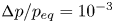 ${\rm \Delta} p/p_{eq}=10^{-3}$ and (b) in the nonlinear regime,
  ${\rm \Delta} p/p_{eq}=15$;
  ${\rm \Delta} R=({{\rm \Delta} p}/{3\gamma p_{eq}})R_{eq}$ is the amplitude of linear undamped oscillations.
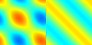
The figure 9 show snapshots of the acoustic pulse  $p(x,t)$ in the liquid in this intermediate regime (
 ${h}/{R_{eq}}=20$) for increasing
  ${\rm \Delta} p$. While the propagation in the liquid is linear, increasing
  ${\rm \Delta} p$ affects the response of the nonlinear oscillator (the screen). It is visible that the signal emitted by the screen, with nonlinear shape, is transmitted to the liquid, in reflection and also, but less visible, in transmission. What is also visible is the fact that increasing the nonlinearities weakens the interaction of the screen with the liquid.

Figure 9. Snapshots of the acoustic pressure in the liquid  ${p(x,t)}/{{\rm \Delta} p}$ for the bubbly screen in a over-damped regime and increasing nonlinearities
  ${{\rm \Delta} p}/{p_{eq}}$ (
 ${h}/{R_{eq}}=20$).
3.1. Analysis in a one-dimensional problem
We shall now simplify the screen model (2.5) to get physical insights into the interaction mechanisms. Restricting ourselves to one-dimensional problem allows for the emergence of a modified RP equation which contains explicitly the radiative damping term and which is independent of the propagation in the liquid; this later will appear as a simple byproduct of the RP solution  $R(t)$. We shall after this consider the harmonic regime for a direct comparison with the model of Leroy et al. (Reference Leroy, Strybulevych, Scanlon and Page2009).
3.1.1. Interpretation in terms of pressure radiated by the screen
One-dimensional propagation involves acoustic pressure of the form  $p(x,t)=p^{inc}(x,t)+f(t\mp {x}/{c_{{\ell }}})$ for
  $x\in {\mathbb {R}}^\pm$. The same function
  $f$ is involved for
  $x\in {\mathbb {R}}^\pm$ since in our problem (2.5) the pressure at
  $x=0$ is continuous; whence
  $f(t)=p(0,t)-p^{inc}(0,t)$. Next, the propagation in the liquid is governed by the Euler equations (2.4a–c) which implies that
  $u_x(x,t)={1}/{\rho _{\ell } c_{\ell }} (p^{inc}(x,t)\pm f(t\mp {x}/{c_{{\ell }}}))$ for
  $x\in {\mathbb {R}}^\pm$. Eventually the jump in the velocity in (2.5) provides
  $f(t)=2{\rm \pi} \rho _{\ell } c_{\ell } ({R^2}/{h^2})\dot {R}$. It follows that the problem (2.4a–c) and (2.5) can be written as
 \begin{align} \left.\begin{gathered} \displaystyle \rho_{\ell}\left(R\ddot R+\frac{3}{2}\dot{R}^2\right)+\frac{\rho_{g} c_{g}^2}{\gamma}\left(1-\left(\frac{R_{eq}}{R}\right)^{\hspace{-.12cm}3\gamma}\right)+\frac{2{\rm \pi} \rho_{\ell} c_{\ell}}{h^2} \,R^2\dot{R}-\frac{\delta \rho_{\ell}}{h}\frac{\textrm{d}\left(R^2\dot{R}\right)}{\textrm{d}t}=-p^{inc}(0,t),\\ \displaystyle p(x,t)=p^{inc}(x,t)+p^{rad}\left(t\mp \frac{x}{c_{\ell}}\right), \quad \text{with}\ p^{rad}(t)=2{\rm \pi}\rho_{\ell} c_{\ell} \frac{R^2(t)\dot{R}(t)}{h^2}, \end{gathered}\right\} \end{align}
for  $x\in {\mathbb {R}}^\pm$ (figure 10). This formulation provides a different although equivalent interpretation of the mechanism of interaction. In a first step, the incident pulse excites the screen;
  $p^{inc}(0,t)$ is the forcing term in the RP equation, (3.2), and it is worth noting that the superradiative damping is now explicitly accounted for by the term in
  $R^2\dot {R}$. In a second step, the screen radiates pressure fluctuations in the liquid, symmetrically on the right and on the left. These fluctuations
  $p^{rad}(t\mp {x}/{c_{\ell }})$, initially generated through a nonlinear mechanism at
  $x=0$, propagate linearly in the liquid; they contain the two time scales, that of the forcing term
  $p^{inc}$ and that of the natural oscillation (under- or over-damped). For our short incident pulse
  $p^{inc}$ the radiated pressure lasts much longer than the pulse as sketched in figure 10. Incidentally, and from a practical point of view, the resolution of (3.2) is simpler than that of (2.4a–c) and (2.5). Indeed, the RP equation is set in time only, hence it can be solved once and for all, and afterwards the solution in the liquid is explicitly known. In figure 10(b), the two numerical solutions of (2.4a–c) and (2.5) and of (3.2) are shown to coincide.

Figure 10. (a) In the one-dimensional problem (3.2), the screen radiates pressure wave trains symmetrically on the right and on the left after the incident signal has passed through it. The solution is the sum of the two contributions  $p=p^{inc}+p^{rad}$ from (3.2). (b) Resulting pressure profiles
  $p$ in the linear and nonlinear regimes, blue lines from (3.2) and dotted red line from the resolution of (2.5).
3.1.2. One-dimensional problem in the linear regime
In the linear regime, with  $R=R_{eq}+r$,
  $r\ll R_{eq}$, (3.2) simplifies further to
 \begin{align} \left.\begin{gathered} \displaystyle \left(1-\frac{\delta R_{eq}}{h}\right)\ddot r+\frac{2{\rm \pi} c_{\ell}}{h^2} R_{eq} \dot{r} +\omega_{M}^2 r=-\frac{p^{inc}(0,t)}{\rho_{\ell}R_{eq}},\\ \displaystyle p(x,t)=p^{inc}(x,t)+p^{rad}\left(t\mp \frac{x}{c_{\ell}}\right), \quad \text{with}\ p^{rad}(t)=2{\rm \pi}\rho_{\ell} c_{\ell} \frac{R_{eq}^2}{h^2}\dot r,\quad \text{for } x\in {\mathbb{R}}^\pm. \end{gathered}\right\} \end{align}
 The analysis can be conducted frequency by frequency by simple Fourier transform. We use  $p^{inc}(x,t)=\int \hat {p}^{inc}(\omega )\exp ({-\textrm {i}(\omega t-kx)})\,\text {d}\omega$ and
  $p^{rad}(t\pm {x}/{c_{\ell }} )=\int \hat p^{rad}(\omega ) \exp ({-\textrm {i}(\omega t\pm kx)})\,\text {d}\omega$, with
  $k={\omega }/{c_{\ell }}$ the wavenumber. The reflection
  ${\mathcal {R}}$ and transmission
  ${\mathcal {T}}$ coefficients read
 \begin{equation} \hat{p}^{rad}(\omega)={\mathcal{R}}(\omega)\hat p^{inc}(\omega)=({\mathcal{T}}(\omega)-1)\hat p^{inc}(\omega),\end{equation}
and  $[\omega _{M}^2-\omega ^2(1-{\delta R _{eq}}/{h} +\textrm {i}KR_{eq})] \hat r=-{\hat p^{inc}}/{\rho _{{\ell }} R_{eq}}$,
  ${\hat p}^{rad}=-\textrm {i}K\rho _{\ell }R_{eq}^2 \omega ^2 \hat {r}$ with
  $K={2{\rm \pi} }/{kh^2}$, hence
 \begin{equation} {\mathcal{R}}(\omega)=\frac{\textrm{i}KR_{eq}}{\left(\dfrac{\omega_{M}}{\omega}\right)^2-1+\dfrac{\delta R_{eq}}{h} -\textrm{i}KR_{eq}}, \quad {\mathcal{T}}(\omega)=1+{\mathcal{R}}(\omega), \end{equation}
with the radiative damping contained in  $KR_{eq}$ and a mass correction contained in
  $\delta ({R_{eq}}/{h})$. (Obviously, the same result for
  $({\mathcal {R}},{\mathcal {T}})$ is found by linearizing (2.5) with
  $u_x=-i/(\rho _{\ell }\omega )\partial _x p$ from (2.4a–c).) As previously said, the damping of the array is much larger than that of an isolated bubble; this latter is given by
  $kR_{eq}$ and we have
  ${k}/{K}=(kh)^2\ll 1$. The mass correction is the product of
  $\delta$ with
  ${R_{eq}}/{h}$. The constant
  $\delta$ depends on the arrangement of the bubbles within the array and it is independent of
  $R_{eq}$ and
  $h$. Hence, for the same arrangement, the mass correction vanishes for sparse arrays
  ${R_{eq}}/{h}\to 0$. From (3.5a,b), the terms of bubble–bubble interaction and of radiative damping vanish for large
  $h$ resulting in
  ${\mathcal {R}}\simeq 0$ (the screen is transparent for the acoustic waves). In the opposite limit of dense arrays
  ${R_{eq}}/{h}\sim 1$, hence
  $KR_{eq} \gg 1$, resulting in
  ${\mathcal {R}}\simeq -1$; the screen becomes equivalent to a wall of air with vanishing acoustic pressure. In the intermediate regime,
  ${\mathcal {R}}$ has a maximum at a frequency
  ${\omega _{M}}/{\sqrt {1-{\delta R_{eq}}/{h}}}$ shifted above the Minnaert frequency as observed in experiments (Leroy et al. Reference Leroy, Strybulevych, Scanlon and Page2009, Reference Leroy, Strybulevych, Lanoy, Lemoult, Tourin and Page2015).
It is worth noting that nonlinearities also produce a shift of the resonance frequency. This is illustrated in figure 11 where we report the Fourier transforms of the reflected and transmitted pressure fields for increasing  ${{\rm \Delta} p}/{p_{eq}} \in (1, 50)$ in our Gaussian pulse (3.1). By analogy with the linear regime, the nonlinear resonance frequency is identified at the maximum in the reflected signal. Expectedly, the frequency shift in the linear regime (
 ${{\rm \Delta} p}/{p_{eq}}=1$) for
  ${h}/{R_{eq}}=40$ is small and we recover (3.4). In the nonlinear regime, the screen imparts to the liquid acoustic pressure fluctuations with complex frequency content. It is in particular visible that (i) for moderate nonlinearities (up to
  ${{\rm \Delta} p}/{p_{eq}}\sim 10$) the shift of the resonance to higher frequency is significantly increased from
  $\omega _{M}$ to approximately
  $3\omega _{M}$ in the reported case, (ii) strong nonlinearities produce the appearance of harmonics and multiple local maxima and minima in the reflection spectrum; in this case, the fundamental resonance is shifted back to
  $\omega _{M}$.

Figure 11. Fourier transforms of the reflected  $\hat p(x<0,\omega )$ and transmitted
  $\hat p(x>0,\omega )$ pressures for increasing nonlinearities
  ${{\rm \Delta} p}/{p_{eq}}$ (
 ${h}/{R_{eq}}=40$).
4. Energy equation
4.1. Conservation of the energy in the screen model
In the absence of viscous loss, the sum of the energy in the liquid and of that in the bubbles is conserved in time. This has to be true in the effective model (2.4a–c) and (2.5) too. To check that this is indeed the case, we consider the equation of energy conservation associated with the Euler equations in the liquid
 \begin{equation} \frac{\textrm{d}}{\textrm{d}t}{\mathcal{E}}+\varPhi=0,\quad \text{with}\ {\mathcal{E}}=\frac{1}{2} \int_\varOmega \left(\frac{p^2}{\rho_{\ell} c_{\ell}^2} +\rho_{\ell} u^2\right)\text{d}{\boldsymbol{r}}\,\text{d}x, \end{equation}
for any bounded domain  $\varOmega$;
  ${\mathcal {E}}$ is the acoustic energy and
  $\varPhi =\int _{\partial \varOmega } p\,{\boldsymbol {u}}\boldsymbol {\cdot } {\boldsymbol {n}} \,\text {d} S$ the flux of the Poynting vector. However, since
  $x=0$ is a surface of discontinuity,
  $\varPhi$ has a contribution
  $\varPhi ^{scr}=-\int _\varGamma p[\kern-1pt[ u_x ]\kern-1pt] \textrm {d}{{\boldsymbol {r}}}$ which from (2.5) reads
 \begin{equation} \varPhi^{scr}=4 {\rm \pi}\int_{x=0} \left[\rho_{\ell}\left(R\ddot R+\frac{3}{2}\dot{R}^2\right)+ \frac{\rho_{g} c_{g}^2}{\gamma}\left(1-\left(\frac{R_{eq}}{R}\right)^{3\gamma}\right)-\frac{\delta\rho_{\ell}}{h} \frac{\partial }{\partial t}\left(R^2\dot{R}\right)\right] R^2 \dot{R}\,\frac{\text{d}{{\boldsymbol{r}}}}{h^2}. \end{equation}
It is easy to see that this flux is the time derivative of an effective energy  $\varPhi ^{scr}=({\textrm {d}}/{\textrm {d}t}) {\mathcal {E}}^{scr}$ with
 \begin{equation} \left.\begin{gathered} {\mathcal{E}}^{scr}=\int_{x=0} \left(e_{p}+e_{c}\right) \frac{\text{d}{{\boldsymbol{r}}}}{h^2},\\ e_{p}=\frac{M_{g}c_{g}^2}{\gamma} \left[\left(\frac{R}{R_{eq}}\right)^3 + \frac{1}{\gamma-1}\left(\frac{R_{eq}}{R}\right)^{3(\gamma-1)}-\frac{\gamma}{\gamma-1}\right],\quad e_{c}= \frac{1}{2}M_{rad} {\dot{R}}^2, \end{gathered}\right\} \end{equation}
where  $e_{p}=0$ at equilibrium (note that, to derive (4.3), we used notably that
  ${\textrm {d}}/{\textrm {d}t} ( R^{{3}/{2}}\dot {R} )^2=2R^2\dot {R} (R\ddot R+\frac {3}{2}\dot {R}^2)$), and
 \begin{equation} M_{g}=\frac{4{\rm \pi}}{3} \rho_{g} R_{eq}^3, \quad M_{rad}=4{\rm \pi} \rho_{\ell} R^3\left(1-\delta\frac{R}{h}\right). \end{equation}
Here,  $M_{g}$ is the (constant) mass of a bubble and
  $M_{rad}$, sometimes termed the ‘radiation mass’, is the effective, or dynamic, mass obtained in the linear regime in (3.3). Expectedly, the effective energy is similar to the classical energy of a single bubble in an incompressible liquid, with
 \begin{equation} e_{p}=- \int_{R_{eq}}^R p (4{\rm \pi} R'^2\,\text{d}R'), \quad\text{with } p=p_{eq}\left(\left(\frac{R_{eq}}{R}\right)^{3\gamma}-1\right) \end{equation}
the work necessary to change the bubble radius from  $R_{eq}$ to
  $R$. Next,
  $e_{c}$ is the kinetic energy invested in a (incompressible) liquid during bubble oscillations; it takes the form
  $e_{c} =\frac {1}{2} \int _R^\infty u^2(4{\rm \pi} \rho _{\ell } r^2\,\textrm {d}r)$ for an isolated bubble. For the array, it can be written
 \begin{equation} e_{c} =\frac{1}{2} \int_R^{{h}/{\delta}} u^2(4{\rm \pi} \rho_{\ell} r^2 \,\textrm{d}r),\quad \text{with } {\boldsymbol{u}}=\frac{R^2\dot{R}}{r^2}\,{{\boldsymbol{e}}}_r, \end{equation}
where we recover the cutoff distance  ${h}/{\delta }$ introduced by Weston (Reference Weston1966) and Leroy et al. (Reference Leroy, Strybulevych, Scanlon and Page2009). Recent works discuss the conservation of energy for a compressible liquid, see e.g. Devaud et al. (Reference Devaud, Hocquet, Bacri and Leroy2008) and Wang (Reference Wang2016), and the effects of confinement (Leighton Reference Leighton2011). As in these references, we find that the energy which is conserved is not the ‘local energy’
  ${\mathcal {E}}^{scr}$ of the bubbles; the liquid and the bubbles can exchange energy hence, in the absence of viscous losses, only
  $({\mathcal {E}}^{scr}+{\mathcal {E}})$ is conserved.
We report in figure 12(a) an example of the time variations of  ${\mathcal {E}}^{scr}(t)$ along with those of
  ${\mathcal {E}}_{R}$ (reflected, i.e. computed in
  $x<0$) and
  ${\mathcal {E}}_{T}$ (transmitted, i.e. computed in
  $x>0$) in the linear regime. In (4.1)
  ${\mathcal {E}}={\mathcal {E}}_{R}+{\mathcal {E}}_{T}$ is the energy in the liquid and the energy conservation applies to
  $({\mathcal {E}}+{\mathcal {E}}^{scr})$. In agreement with the snapshots in the figure 8(a), the screen takes a significant part of the acoustic energy during the transit of the incident pulse, up to 40 % of the total energy in the reported case. It then releases this energy over a time which scales with
  $T$. In the present case, the regime is over-damped and the energy release varies as
  ${\sim }\exp (-5.6 ({t}/{T}))$, in agreement with (3.3) (
 ${\delta R _{eq}}/{h}\simeq 0.2$,
  $KR_{eq}\simeq 2.4$). Panels (b,c) further quantify the influence of the array spacing and of the nonlinearities. We have considered a sufficiently large time so that almost all the energy is in the liquid. As previously said, going from sparse to dense array increasing
  ${h}/{R_{eq}}$ produces a transition from a perfect shield (total reflection) to a transparent screen (total transmission). Next, incident signals with high nonlinearities are less sensitive to the screen; for
  ${{\rm \Delta} p}/{p_{eq}}$ larger than approximately 50, the reflected energy
  ${\mathcal {E}}_{R}$ is negligible.

Figure 12. Normalized energies. (a) Example of time variations of  ${\mathcal {E}}_{R}$ and
  ${\mathcal {E}}_{T}$ (energies in the liquid, computed for
  $x<0$ and
  $x>0$, with
  ${\mathcal {E}}={\mathcal {E}}_{R}+{\mathcal {E}}_{T}$ in (4.1)), and
  ${\mathcal {E}}^{scr}$ from (4.3); grey dashed line shows
  $({\mathcal {E}}+{\mathcal {E}}^{scr})\simeq 1$ (
 $h/R_{eq}=20$,
  ${\rm \Delta} p/p_{eq}=10^{-3}$); (b)
  ${\mathcal {E}}_{R}$ and
  ${\mathcal {E}}_{T}$ against
  $h/R_{eq}$ in the linear regime (
 ${\rm \Delta} p/p_{eq}=10^{-3}$); (c)
  ${\mathcal {E}}_{R}$ and
  ${\mathcal {E}}_{T}$ against
  ${\rm \Delta} p/p_{eq}$ (
 $h/R_{eq}=20$).
5. Concluding remarks
We have derived an effective model which aims to reproduce the scattering properties of a bubbly screen with resonances of the Minnaert type. The model enables to reduce the effect of the screen to a jump of the acoustic velocity in the liquid coupled to a modified RP equation. The RP equation contains the super-radiative damping of the array being much larger than the classical damping of an isolated bubble. Next, a more significant result is the derivation of the term of bubble–bubble interaction in the RP equation dictating the nonlinear dynamics of the array. This contribution was absent from the analysis of Caflisch et al. (Reference Caflisch, Miksis, Papanicolaou and Ting1985a,Reference Caflisch, Miksis, Papanicolaou and Tingb) for a bubbly liquid and its extension to a bubbly screen (Ng & Ting Reference Ng and Ting1986; Miksis & Ting Reference Miksis and Ting1989); indeed its derivation requires the analysis to be conducted one order further than the dominant one considered in these references. Our result generalizes the findings of Leroy et al. (Reference Leroy, Strybulevych, Scanlon and Page2009) to the nonlinear regime and to the time domain. It was shown that this contribution was able to describe the shift in the resonance frequency to the higher frequency observed experimentally (Leroy et al. Reference Leroy, Strybulevych, Scanlon and Page2009, Reference Leroy, Strybulevych, Lanoy, Lemoult, Tourin and Page2015; Lanoy et al. Reference Lanoy, Guillermic, Strybulevych and Page2018); we have stressed that this tendency can be significantly accentuated in the weakly nonlinear regime and inverted with the occurrence of harmonics.
Some extensions of the present work are easy, some others are more tricky. We have neglected the effects of surface tension and viscosity; as in Schnitzer et al. (Reference Schnitzer, Brandão and Yariv2019), this is partially justified by the large, dominant, radiative damping of the array. However, there are no particular difficulties in including them, as has been done in Caflisch et al. (Reference Caflisch, Miksis, Papanicolaou and Ting1985a,Reference Caflisch, Miksis, Papanicolaou and Tingb), and there is little doubt that this will affect the Rayleigh–Plesset equation only. This may become necessary, for instance to explain the perfect absorption by critical coupling (a balance between viscous loss and radiative damping) studied by Lanoy et al. (Reference Lanoy, Guillermic, Strybulevych and Page2018). It is also straightforward to account for different arrangements within the array which would affect the mesoscopic solution by modifying the cross-section of the unit cell for the Green's function in (2.9). Next, accounting for different shape of the bubbles would affect the microscopic solution, namely the response of a single bubble e.g. a disk with monopolar resonance (Calvo et al. Reference Calvo, Thangawng, Layman, Casalini and Othman2015). Following Ammari et al. (Reference Ammari, Fitzpatrick, Gontier, Lee and Zhang2017a, Reference Ammari, Fitzpatrick, Gontier, Lee and Zhang2018, Reference Ammari, Fitzpatrick, Hiltunen, Lee and Yu2019), it should be possible to extend our present work to any geometry. The case of arrays of cylindrical bubbles involved in anechoic tiles, see e.g. Hladky-Hennion & Decarpigny (Reference Hladky-Hennion and Decarpigny1991) and Sharma et al. (Reference Sharma, Skvortsov, MacGillivray and Kessissoglou2017), with a long or infinite length in one direction is slightly more involved but of interest; it requires us to use a different scaling adapted to the two-dimensional problem, as done in Schnitzer et al. (Reference Schnitzer, Brandão and Yariv2019). For this application, accounting in addition for a viscoelastic matrix rather than for a liquid may be quite involved depending on the considered viscoelastic model. Next, a different extension concerns the case of bubbly liquids. Pursuing the analysis of Caflisch et al. (Reference Caflisch, Miksis, Papanicolaou and Ting1985a,Reference Caflisch, Miksis, Papanicolaou and Tingb), and using the mathematical framework of Ammari & Zhang (Reference Ammari and Zhang2017), Ammari et al. (Reference Ammari, Fitzpatrick, Gontier, Lee and Zhang2017b), would provide the bubble–bubble interaction in these media by use of a Green's function that is periodic in the three directions; this would allow us to test the validity of (1.1) and in particular to inspect under which circumstances the dynamic mass  $M_{rad}$ in (4.4a,b) is higher or lower than the actual bubble mass (
 $\delta$ positive or negative). Eventually, we have assumed that the transformations undergone by the gas are adiabatic and the result holds for isothermal transformations by simply setting
  $\gamma =1$. A much more challenging extension is to account for the thermal exchanges between the gas and the liquid since the whole asymptotic analysis has to be reconsidered including the complete thermodynamics.
Acknowledgements
K.P., J.-F.M. and A.M. thank V. Leroy for fruitful discussions. K.P. thanks the support of the Agence de l'Innovation de Défense (AID) from the Direction Générale de l'Armement (DGA), under grant 2019 65 0070.
Declaration of interests
The authors report no conflict of interest.
Appendix A. Asymptotic analysis
In this appendix, we shall use non-dimensional variables  $t\to \omega t$ and
  ${{\boldsymbol {x}}} \to ({\omega }/{c_{\ell }}){{\boldsymbol {x}}}$ (with
  ${{\boldsymbol {x}}}=(x,{{\boldsymbol {r}}})$), where
  $\omega$ is the typical frequency imposed by the source. Denoting by
  $U_{a}$ the amplitude of the acoustic velocity, we have, from (2.1a–c) and (2.2),
  $u\sim U_{a}$,
  $p\sim \rho _{\ell } c_{\ell } U_{a}$,
  $(\rho -\rho _{\ell }) \sim ({\rho _{\ell }}/{c_{\ell }}) U_{a}$. With
  $Ma={U_{a}}/{c_{\ell }}$ the Mach number, we shall use dimensionless quantities
 \begin{equation} p\to \frac{1}{\rho_{\ell} c_{\ell}^2\,Ma} p,\quad \rho\to \frac{1}{\rho_{\ell}Ma} \left(\rho-\rho_{{\ell},{g}}\right),\quad {{\boldsymbol{u}}} \to\frac{1}{c_{\ell} Ma}\,{\boldsymbol{u}},\quad R\to \frac{R}{R_{eq}}. \end{equation}
Note that the bubble radius is not assumed to scale with the Mach number. This choice prevents a simple linear response where the solution would be proportional to  $Ma$. In the low frequency regime, the maximum wavelength imposed by the source is much larger than
  $h$ and
  $R_{eq}$; this is accounted for with
  $\varepsilon =({\omega }/{c_{\ell }}) h \ll 1$. Next, we impose the following scalings:
 \begin{equation} \frac{\omega}{c_{{\ell}}} R_{eq}={\boldsymbol{\mathsf{r}}}_{eq}\varepsilon^2,\quad \frac{\rho_{g}}{\rho_{\ell}}=\alpha \varepsilon^4,\quad \frac{\rho_{g}c_{g}^2}{\rho_{\ell}c_{\ell}^2}=\beta\varepsilon^4,\quad Ma= m \varepsilon^4. \end{equation}
Doing so, we assume that the bubbly screen is dilute since  ${R_{eq}}/{h}=O(\varepsilon )$. Such separation of scales was already used in Caflisch et al. (Reference Caflisch, Miksis, Papanicolaou and Ting1985b) for bubbly liquid, and in this case, the separation was even more demanding with
  ${R_{eq}}/{h}=O(\varepsilon ^2)$. The Minnaert resonance is dictated by the contrast in the mass densities only, hence, we set
  ${\rho _{g}}/{\rho _{\ell }}=O(\varepsilon ^4)$ and
  ${c_{g}}/{c_{\ell }}=O(1)$. The scalings are such that the resonance takes place in the low frequency regime, specifically
  ${\omega _{M} h}/{c_{\ell }}=O(\varepsilon )$. Eventually, the scaling for the Mach number produces a linear propagation of waves at large scale in the liquid while keeping nonlinear responses of the bubbles, see Lombard, Barrière & Leroy (Reference Lombard, Barrière and Leroy2015). The asymptotic analysis requires the use of the rescaled dimensionless coordinates
  ${{\boldsymbol {x}}}$ at the macroscopic scale of the wavelength,
  ${{\boldsymbol {x}}}_{m}$ at the mesoscopic scale of the array spacing and
  ${{\boldsymbol {x}}}_{\mu }$ at the microscopic scale of the bubble radius (figure 13), with
 \begin{equation} \left.\begin{gathered} \displaystyle {{\boldsymbol{x}}}, \quad {{\boldsymbol{x}}}=(x,{{\boldsymbol{r}}})\in\mathbb{R}^3,\\ \displaystyle{{\boldsymbol{x}}}_{m}=\frac{{{\boldsymbol{x}}}}{\varepsilon}, \quad \displaystyle {{\boldsymbol{x}}}_{m}=(x_{m},{{\boldsymbol{r}}}_{m})\in {\mathcal{Y}},\ {\mathcal{Y}}= \left\{x_{m}\in \mathbb{R}, {{\boldsymbol{r}}}_{m}\in {\boldsymbol{\mathsf{Y}}}\right\}, {\boldsymbol{\mathsf{Y}}}=\left(-\frac{1}{2},\frac{1}{2}\right)^2,\\ \displaystyle {{\boldsymbol{x}}}_{\mu}=\frac{1}{{\boldsymbol{\mathsf{r}}}_{eq}R({{\boldsymbol{r}}},t)}\,\frac{{{\boldsymbol{x}}}}{\varepsilon^2}, \quad \displaystyle {{\boldsymbol{x}}}_{\mu} \in \mathbb{R}^3. \end{gathered}\right\} \end{equation}
Figure 13. The separation of the scales – at the microscopic scale, the problem is that of a single bubble with a radius of unity in a liquid with  ${{\boldsymbol {x}}}_{\mu }\in {\mathbb {R}}^3$. At the mesoscopic scale, the bubble is reduced to a singularity within a periodic cell
  ${\mathcal {Y}}$ with
  ${{\boldsymbol {x}}}_{m}=x_{m}{{\boldsymbol {e}}}_x+{\boldsymbol {r}}_{m}$,
  $x_{m}\in {\mathbb {R}}$ and
  ${\boldsymbol {r}}_{m}\in {\boldsymbol{\mathsf{Y}}}$,
  ${\boldsymbol{\mathsf{Y}}}=(-\frac {1}{2},\frac {1}{2})^2$. At the final, macroscopic scale the whole bubbly screen is reduced to an effective screen at
  $x=0$ across which jump conditions apply (with
  ${{\boldsymbol {x}}}=x{{\boldsymbol {e}}}_x+{{\boldsymbol {r}}}$,
  ${{\boldsymbol {x}}}\in {\mathbb {R}}^2$).
A.1. Non-dimensional form of the problem
The problem (2.1a–c) and (2.2) now reads as
 \begin{equation} \text{in the gaz:}\quad \left\{\begin{aligned} &\displaystyle \dfrac{\partial \rho}{\partial t}+ \varepsilon^4 \left(\alpha \,{\rm div} \,{{\boldsymbol{u}}}+ m \,{\rm div} (\rho {{\boldsymbol{u}}})\right)=0,\quad \displaystyle 1+\dfrac{\gamma m}{\beta} \,p=\left(1+\dfrac{m}{\alpha} \,\rho\right)^\gamma,\\ &\displaystyle \varepsilon^4(\alpha +m \rho) \left(\dfrac{\partial {{\boldsymbol{u}}}}{\partial t} + \varepsilon^4 m({{\boldsymbol{u}}} \boldsymbol{\cdot} \boldsymbol{\nabla}){{\boldsymbol{u}}} \right)=- {\boldsymbol{\nabla}} p,\quad \displaystyle \boldsymbol{\nabla} \land {{\boldsymbol{u}}} = 0, \end{aligned}\right. \end{equation}
 \begin{equation}\text{in the liquid:}\quad \left\{\begin{aligned} &\displaystyle \dfrac{\partial \rho}{\partial t}+{\rm div}\,{{\boldsymbol{u}}} + m \varepsilon^4 \,{\rm div}(\rho {{\boldsymbol{u}}})=0,\quad p=\rho,\\ &\displaystyle \left(1 + \varepsilon^4m \rho\right) \left(\dfrac{\partial {{\boldsymbol{u}}}}{\partial t} + \varepsilon^4 m ({{\boldsymbol{u}}} \boldsymbol{\cdot} \boldsymbol{\nabla}) {{\boldsymbol{u}}} \right)=- {\boldsymbol{\nabla}} p,\quad \displaystyle \boldsymbol{\nabla} \land {{\boldsymbol{u}}} = 0, \end{aligned} \right. \end{equation}
with initial conditions (i.c.) and boundary conditions at the bubble interface (b.c.)
 \begin{equation} \left.\begin{gathered} \text{i.c.} \quad p({{\boldsymbol{x}}},0)=0,\quad \rho({{\boldsymbol{x}}},0)=0 ,\quad {{\boldsymbol{u}}}({{\boldsymbol{x}}},0)=\textbf{{0}},\\ \text{b.c.}\quad p,\ {{\boldsymbol{u}}}\boldsymbol{\cdot} {\boldsymbol{n}}\ \text{are continuous and}\ \displaystyle {{\boldsymbol{u}}}\boldsymbol{\cdot}{\boldsymbol{n}}= \frac{1}{\varepsilon^2}\frac{{\boldsymbol{\mathsf{r}}}_{eq}}{m}\,\dot{R}. \end{gathered}\right\} \end{equation}
A.2. Derivation of effective transmission conditions at the dominant order
The separation of the scales requires the asymptotic analysis to be performed at three scales, the microscopic scale being that of a single bubble, the mesoscopic scale of the array where the bubbles are reduced to points and eventually the macroscopic scale of the waves, the scale at which the whole screen is reduced to an interface  $x=0$ (figure 2).
A.2.1. Order 0 – resolution at the microscopic scale: the scale of the bubble
The microscopic scale is the scale corresponding to a zoom on a single bubble at a given time  $t$. At this scale, the spherical coordinate
  ${{\boldsymbol {x}}}_{\mu }=({1}/{{\boldsymbol{\mathsf{r}}}_{eq}R({{\boldsymbol {r}}},t)}){{{\boldsymbol {x}}}}/{\varepsilon ^2}$ (see (A 3)) where, following Caflisch et al. (Reference Caflisch, Miksis, Papanicolaou and Ting1985b), the discrete version of the bubble radius
  $R_i$ (see e.g. (2.3)) has been replaced by a continuous counterpart
  $R({{\boldsymbol {r}}},t)$. Doing so, the bubble has a unitary radius and the nearby bubbles have been sent to infinity. We consider the following expansions of the solution in the gas:
 \begin{equation} \left.\begin{gathered} {{\boldsymbol{u}}}=\dfrac{1}{\varepsilon^2}\hat{\boldsymbol{u}}_{\mu}^{-2}({{\boldsymbol{x}}}_{\mu},{{\boldsymbol{r}}},t)+\dfrac{1}{\varepsilon} \hat{\boldsymbol{u}}_{\mu}^{-1}({{\boldsymbol{x}}}_{\mu},{{\boldsymbol{r}}},t)\cdots,\quad p=\hat{p}_{\mu}^0({{\boldsymbol{x}}}_{\mu},{{\boldsymbol{r}}},t)+\varepsilon \hat{p}_{\mu}^1({{\boldsymbol{x}}}_{\mu},{{\boldsymbol{r}}},t)+\cdots,\\ \rho=\hat{\rho}_{\mu}^0({{\boldsymbol{x}}}_{\mu},{{\boldsymbol{r}}},t)+\varepsilon \hat{\rho}_{\mu}^1({{\boldsymbol{x}}}_{\mu},{{\boldsymbol{r}}},t)+\cdots,\quad R=R^0({{\boldsymbol{r}}},t)+\varepsilon R^1({{\boldsymbol{r}}},t)+\cdots, \end{gathered}\right\} \end{equation}
and in the liquid (where  $p=\rho$)
 \begin{equation} {{\boldsymbol{u}}}=\displaystyle\frac{1}{\varepsilon^2}{\boldsymbol{u}}_{\mu}^{-2}({{\boldsymbol{x}}}_{\mu},{{\boldsymbol{r}}},t)+\frac{1}{\varepsilon} {\boldsymbol{u}}_{\mu}^{-1}({{\boldsymbol{x}}}_{\mu},{{\boldsymbol{r}}},t)+\cdots, \quad p=p_{\mu}^0({{\boldsymbol{x}}}_{\mu},{{\boldsymbol{r}}},t)+\varepsilon p_{\mu}^1({{\boldsymbol{x}}}_{\mu},{{\boldsymbol{r}}},t)+\cdots. \end{equation}
Accordingly, denoting  ${{\boldsymbol {\nabla }}}_{\mu }\,=\partial /\partial \boldsymbol {x}_{\mu }$ and
  ${\boldsymbol {\nabla }}_{{{\boldsymbol {r}}}}=\partial /\partial \boldsymbol {r}$, the differential operators read
 \begin{equation} {\boldsymbol{\nabla}} \to \displaystyle \frac{1}{{\boldsymbol{\mathsf{r}}}_{eq}R} \frac{{{\boldsymbol{\nabla}}}_{\mu}\, }{\varepsilon^2} +{\boldsymbol{\nabla}}_{{{\boldsymbol{r}}}}- \frac{{\boldsymbol{\nabla}}_{{{\boldsymbol{r}}}} R}{R}\, {{\boldsymbol{x}}}_{\mu} \boldsymbol{\cdot} {{\boldsymbol{\nabla}}}_{\mu}\,\quad \text{and} \quad \displaystyle \frac{\partial}{\partial t} \to \displaystyle \frac{\partial}{\partial t}-\frac{\dot{R}}{R} \,{{\boldsymbol{x}}}_{\mu} \boldsymbol{\cdot} {{\boldsymbol{\nabla}}}_{\mu}\,. \end{equation}
 Resolution inside the bubble – using the expansions (A 7) in (A 4) along with (A 9), the problem at the dominant order gives uniform pressure and mass density with  ${{\boldsymbol {\nabla }}}_{\mu }\, \hat {p}_{\mu }^0 = 0$ and
 \begin{align} \displaystyle \frac{\partial \hat{\rho}_{\mu}^0}{\partial t} +\frac{\left(\alpha + m\hat{\rho}_{\mu}^0\right)}{{\boldsymbol{\mathsf{r}}}_{eq}R^0}\,\text{div}_{\mu}\, \hat{\boldsymbol{u}}_{\mu}^{-2}=0,\quad \boldsymbol{\nabla} \land \hat{\boldsymbol{u}}_{\mu}^{-2} = 0, \quad 1+\gamma\frac{m}{\beta} \hat{p}_{\mu}^0=\left(1+\frac{m}{\alpha} \hat{\rho}_{\mu}^0\right)^\gamma, \end{align}
and initial and boundary conditions, from (A 6), of the form
 \begin{equation} \left.\begin{gathered}{}{\rm i.c.\quad at } t=0,\quad \hat{p}_{\mu}^0=\hat{\rho}_{\mu}^0=0, \quad \hat{\boldsymbol{u}}_{\mu}^{-2}=\textbf{{0}}, \quad R^0=1,\\ {\rm b.c.\quad for } |{{\boldsymbol{x}}}_{\mu}|=1,\quad \displaystyle \hat{p}_{\mu}^0=p_{\mu}^0, \quad \hat{\boldsymbol{u}}_{\mu}^{-2}\boldsymbol{\cdot} {{\boldsymbol{e}}}_r= \frac{{\boldsymbol{\mathsf{r}}}_{eq}}{m}\, \dot{R}^0, \end{gathered}\right\} \end{equation}
where  ${{\boldsymbol {e}}}_r={{\boldsymbol {x}}}_{\mu }/|{{\boldsymbol {x}}}_{\mu }|$. Now, we shall express
  $\hat {p}_{\mu }^0({{\boldsymbol {r}}},t)$ and
  $\hat {\rho }_{\mu }^0({{\boldsymbol {r}}},t)$ as a function of
  $R^0({{\boldsymbol {r}}},t)$. By integrating the balance of mass over the gas bubble (first equation in (A 10a–c)) we get
  $({4{\rm \pi} }/{3})(\partial\hat {\rho }_{\mu }^0/\partial t)+(\alpha + m\hat {\rho }_{\mu }^0)({1}/{{\boldsymbol{\mathsf{r}}}_{eq}R^0})\int _{|{{\boldsymbol {x}}}_{\mu }|=1} \hat {\boldsymbol {u}}_{\mu }^{-2}\boldsymbol {\cdot } {{\boldsymbol {e}}}_r\, \text {d}s=0$. This differential equation on
  $\hat {\rho }_{\mu }^0$ is solved using in (A 11) (i) the boundary condition on
  $\hat {\boldsymbol {u}}_{\mu }^{-2}$ and (ii) the initial conditions
  $\hat {\rho }_{\mu }^0=0$,
  $R^0=1$ at
  $t=0$. Also, making use of the equation of state in (A 10a–c), we obtain the pressure
  $\hat {p}_{\mu }^0$. Eventually, the velocity
  $\hat {\boldsymbol {u}}_{\mu }^{-2}$ is a byproduct of
  $\hat {\rho }_{\mu }^0$ in (A 10a–c). The result is
 \begin{equation} \left.\begin{gathered} \hat{\rho}_{\mu}^0({{\boldsymbol{r}}},t)=\frac{\alpha}{m} \left(\frac{1}{(R^0)^3}-1\right),\quad \hat{p}_{\mu}^0({{\boldsymbol{r}}},t)=\frac{\beta}{\gamma m}\left(\frac{1}{(R^0)^{3\gamma}} -1\right),\\ \hat{\boldsymbol{u}}_{\mu}^{-2}({{\boldsymbol{x}}}_{\mu},{{\boldsymbol{r}}},t)=\frac{{\boldsymbol{\mathsf{r}}}_{eq}}{m} \dot{R}^0 |{{\boldsymbol{x}}}_{\mu}|\,{{\boldsymbol{e}}}_r, \end{gathered}\right\} \end{equation}
given in dimensional form in (2.7).
Resolution in the liquid – in the liquid, we repeat the exercise, using the expansions (A 8) in (A 5) and (A 6) along with (A 9). We get at the dominant order
 \begin{equation} \left.\begin{array}{c} \displaystyle \text{div}_{\mu}\, {\boldsymbol{u}}_{\mu}^{-2}=0, \quad {{\boldsymbol{\nabla}}}_{\mu}\, \land {\boldsymbol{u}}_{\mu}^{-2} = 0,\\ \displaystyle \dfrac{\partial{\boldsymbol{u}}_{\mu}^{-2}}{\partial t} +\dfrac{m}{{\boldsymbol{\mathsf{r}}}_{eq}R^0} ({\boldsymbol{u}}_{\mu}^{-2} \boldsymbol{\cdot} {{\boldsymbol{\nabla}}}_{\mu}\,) {\boldsymbol{u}}_{\mu}^{-2}-\dfrac{\dot{R}^0}{R^0}\,{{\boldsymbol{x}}}_{\mu} \boldsymbol{\cdot} {{\boldsymbol{\nabla}}}_{\mu}\,{\boldsymbol{u}}_{\mu}^{-2}=-\dfrac{1}{{\boldsymbol{\mathsf{r}}}_{eq}R^0} {{\boldsymbol{\nabla}}}_{\mu}\, p_{\mu}^0, \end{array} \right\} \end{equation}
with initial and boundary conditions
 \begin{align} \left.\begin{gathered}{} \displaystyle \text{i.c.}\quad \text{at }t=0, \quad p_{\mu}^0=0, \quad {\boldsymbol{u}}_{\mu}^{-2}=\textbf{{0}}, \\ \displaystyle \text{b.c.}\quad \text{for } |{{\boldsymbol{x}}}_{\mu}|=1,\quad {\boldsymbol{u}}_{\mu}^{-2}\boldsymbol{\cdot} {{\boldsymbol{e}}}_r= \dfrac{{\boldsymbol{\mathsf{r}}}_{eq}}{m}\, \dot{R}^0\quad \text{and} \quad \displaystyle \lim_{|{{\boldsymbol{x}}}_{\mu}|\to +\infty} p_{\mu}^0({{\boldsymbol{x}}}_{\mu},{{\boldsymbol{r}}},t)=P^0({{\boldsymbol{r}}},t). \end{gathered}\right\} \end{align}
For the time being, the continuity of the pressure at  $|{{\boldsymbol {x}}}_{\mu }|=1$ is not needed, but we have introduced the (unknown) pressure field
  $P^0({{\boldsymbol {r}}},t)$; its meaning will appear later on. We have also assumed that the bubble remains spherical.
From (A 13), the flow is incompressible and irrotational. Hence it is associated with a velocity potential  $\phi$ and, the bubble remaining spherical,
  ${\phi =({A}/{|{{\boldsymbol {x}}}_{\mu }|})+B}$. Next, the boundary condition in (A 14) for
  ${\boldsymbol {u}}_{\mu }^{-2}={{\boldsymbol {\nabla }}}_{\mu }\, \phi$ provides
  $A=-{{\boldsymbol{\mathsf{r}}}_{eq}\dot {R}^0}/{m}$. Using
  ${\boldsymbol {u}}_{\mu }^{-2}$ in (A 13), the pressure
  $p_{\mu }^0$ is found to satisfy a Bernoulli equation
  ${{\boldsymbol {\nabla }}}_{\mu }\,(p_{\mu }^0+({{\boldsymbol{\mathsf{r}}}_{eq}^2}/{m})\,F(R^0,\dot R^0,\ddot R^0,|{{\boldsymbol {x}}}_{\mu }|))=0$, that we integrate using
  $p_{\mu }^0\to _{|{{\boldsymbol {x}}}_{\mu }|\to +\infty } P^0({{\boldsymbol {r}}},t)$ from (A 14). Doing so, the fields
  $({\boldsymbol {u}}_{\mu }^{-2},p_{\mu }^0)$ are found to be functions of
  $R^0$ and of their time derivatives
 \begin{align} {\boldsymbol{u}}_{\mu}^{-2}({{\boldsymbol{x}}}_{\mu},{{\boldsymbol{r}}},t)=\frac{{\boldsymbol{\mathsf{r}}}_{eq}}{m}\,\frac{\dot{R}^0}{|{{\boldsymbol{x}}}_{\mu}|^2}\, {{\boldsymbol{e}}}_r, \quad p_{\mu}^0({{\boldsymbol{x}}}_{\mu},{{\boldsymbol{r}}},t)=P^0+\frac{{\boldsymbol{\mathsf{r}}}_{eq}^2}{m} \left(\frac{R^0\ddot{R}^0+2(\dot{R}^0)^2}{|{{\boldsymbol{x}}}_{\mu}|}- \frac{(\dot{R}^0)^2}{2|{{\boldsymbol{x}}}_{\mu}|^4}\right), \end{align}
given in dimensional form in (2.7). At this stage, once  $R^0({{\boldsymbol {r}}},t)$ is known, the solution in the bubble is known from (A 12a–c), and the solution in the liquid is known up to the pressure field
  $P^0({{\boldsymbol {r}}},t)$ from (A 15a,b).
An equation of the Rayleigh–Plesset type – we shall establish that  $R^0({{\boldsymbol {r}}},t)$ satisfies a continuous version of the Rayleigh–Plesset equation. To do so, we use
  $p_{\mu }^0=\hat {p}_{\mu }^0$ for
  ${|{{\boldsymbol {x}}}_{\mu }|=1}$, with
  $\hat {p}_{\mu }^0$ in (A 12a–c) and
  $p_{\mu }^0$ in (A 15a,b). We get that
  $R^0({{\boldsymbol {r}}},t)$ is solution of
 \begin{equation} R^0\ddot{R}^0+\frac{3}{2}(\dot{R}^0)^2+\frac{\beta}{\gamma {\boldsymbol{\mathsf{r}}}_{eq}^2}\left(1-\frac{1}{(R^0)^{3\gamma}}\right)=-\frac{m}{{\boldsymbol{\mathsf{r}}}_{eq}^2} P^0({{\boldsymbol{r}}},t) \end{equation}
and at the equilibrium  $P^0=0$, the bubbles and the liquid are at rest and the acoustic pressures vanish (
 $R^0=1$ in (A 16) hence,
  ${\boldsymbol {u}}_{\mu }^{-2}=\textbf {{0}}$ and
  $\hat {p}_{\mu }^0=p_{\mu }^0=0$ in (A 15a,b)).
A.2.2. Order 0 – resolution at the mesoscopic scale: the scale of the screen spacing
From (A 12a–c), (A 15a,b) and (A 16), the solution at the microscopic scale is known once  $P^0({{\boldsymbol {r}}},t)$ is known, and
  $P^0$ will be provided by the mesoscopic problem. This scale is that of the array spacing, intermediate between the bubble size and the wavelength. It is associated with
  ${{\boldsymbol {x}}}_{m}={{{\boldsymbol {x}}}}/{\varepsilon }$,
  ${{\boldsymbol {x}}}_{m}=(x_{m},{{\boldsymbol {r}}}_{m})$ defined in (A 3), and we use the expansions
 \begin{align} \left.\begin{gathered} \displaystyle{{\boldsymbol{u}}}={\boldsymbol{u}}_{m}^0({{\boldsymbol{x}}}_{m},{{\boldsymbol{r}}},t)+\varepsilon {\boldsymbol{u}}_{m}^1({{\boldsymbol{x}}}_{m},{{\boldsymbol{r}}},t)+\cdots,\\ p=p_{m}^0({{\boldsymbol{x}}}_{m},{{\boldsymbol{r}}},t)+\varepsilon p_{m}^1({{\boldsymbol{x}}}_{m},{{\boldsymbol{r}}},t)+\cdots,\quad \rho=\rho_{m}^0({{\boldsymbol{x}}}_{m},{{\boldsymbol{r}}},t)+\varepsilon \rho_{m}^1({{\boldsymbol{x}}}_{m},{{\boldsymbol{r}}},t)+\cdots, \end{gathered}\right\} \end{align}
where the  $({\boldsymbol {u}}_{m}^i,p_{m}^i,\rho _{m}^i)$,
  $i=0,1,\ldots$ are periodic with respect to
  ${{\boldsymbol {r}}}_{m}\in {\boldsymbol{\mathsf{Y}}}$. In
  ${{\boldsymbol {x}}}_{m}$-coordinate, denoting
  ${\boldsymbol {\nabla }}_{{m}}\,=\partial /\partial \boldsymbol {x}_{m}$ (and
  ${\boldsymbol {\nabla }}_{{{\boldsymbol {r}}}}=\partial /\partial \boldsymbol {r}$ as in (A 9)), the differential operators read
 \begin{equation} {\boldsymbol{\nabla}} \to \displaystyle \frac{1}{\varepsilon} {\boldsymbol{\nabla}}_{{m}}\, +{\boldsymbol{\nabla}}_{{{\boldsymbol{r}}}}, \quad \frac{\partial}{\partial t} \to \displaystyle \frac{\partial}{\partial t}. \end{equation}
 Matching conditions – the matching conditions tell us that the solution of the microscopic problem has to coincide with that of the mesoscopic problem in some intermediate region, when  $|{{\boldsymbol {x}}}_{\mu }|\to +\infty$ and
  ${{\boldsymbol {x}}}_{m} \to 0$. Since
  $|{{\boldsymbol {x}}}_{m}|=O({|{{\boldsymbol {x}}}|}/{\varepsilon })$ and
  $|{{\boldsymbol {x}}}_{\mu }|=O({|{{\boldsymbol {x}}}|}/{\varepsilon ^2})$, this intermediate region can be sought at distance
  $\varepsilon \sqrt {\varepsilon }$ of the bubble, in
  ${{\boldsymbol {x}}}$ coordinate; hence,
  $|{{\boldsymbol {x}}}_{\mu }|\sim {1}/{\sqrt {\varepsilon }}$ and
  $|{{\boldsymbol {x}}}_{m}|\sim \sqrt {\varepsilon }$. The matching conditions are obtained by identifying the expansions (A 7) and (A 17) for
  ${{\boldsymbol {x}}}_{\mu }={{{\boldsymbol {x}}}_{m}}/{\varepsilon {\boldsymbol{\mathsf{r}}}_{eq}R}$ and
  ${{\boldsymbol {x}}}_{m}\to 0$. At the dominant order, anticipating that
  $p_{m}^0$ does not depend on
  ${{\boldsymbol {x}}}_{m}$, we get
 \begin{equation} \displaystyle p_{m}^0({{\boldsymbol{r}}},t)\!+\cdots \sim p_{\mu}^0\left(\frac{{{\boldsymbol{x}}}_{m}}{{\boldsymbol{\mathsf{r}}}_{eq}\varepsilon R},{{\boldsymbol{r}}},t\right)\!+\cdots, \quad \displaystyle {\boldsymbol{u}}_{m}^{0}({{\boldsymbol{x}}}_{m},{{\boldsymbol{r}}},t)+\cdots \sim \frac{1}{\varepsilon^2}{\boldsymbol{u}}_{\mu}^{-2}\left(\frac{{{\boldsymbol{x}}}_{m}}{{\boldsymbol{\mathsf{r}}}_{eq}\varepsilon R},{{\boldsymbol{r}}},t\right) \!+\cdots \end{equation}
for  ${{\boldsymbol {x}}}_{m}\to \textbf {{0}}$, hence
 \begin{align} \lim_{|{{\boldsymbol{x}}}_{\mu}|\to +\infty} p_{\mu}^0({{\boldsymbol{x}}}_{\mu},{{\boldsymbol{r}}},t)=p_{m}^0({{\boldsymbol{r}}},t)=P^0({{\boldsymbol{r}}},t),\quad \displaystyle {\boldsymbol{u}}_{m}^0({{\boldsymbol{x}}}_{m},{{\boldsymbol{r}}},t) \underset{ {{\boldsymbol{x}}}_{m} \to \textbf{{0}}}{\sim} \frac{{\boldsymbol{\mathsf{r}}}_{eq}^3}{m} (R^0)^2\dot{R}^0\,\frac{{{\boldsymbol{x}}}_{m}}{ |{{\boldsymbol{x}}}_{m}|^3}. \end{align}
 We have used  ${\boldsymbol {u}}_{\mu }^{-2}$ in (A 15a,b) and we have assumed that the terms
  ${\boldsymbol {u}}_{\mu }^{n}$, when increasing
  $n>-2$, decrease faster than
  ${\boldsymbol {u}}_{\mu }^{-2}\propto {1}/{|{{\boldsymbol {x}}}_{\mu }|^2}$, which is consistent with non-diverging mass flux through a spherical cap. It follows that the main results provided by the mesoscopic problem are: the pressure
  $\tilde {P}^0({{\boldsymbol {r}}},t)$ introduced in (A 14) is the pressure
  $p_{m}^0$ at
  $|{{\boldsymbol {x}}}_{m}|=0$ (at the mesoscopic scale, the bubbles are reduced to points), the velocity
  ${\boldsymbol {u}}_{m}^0$ is singular at the origin, and it encapsulates the effect of the oscillating bubble point (if
  $\dot R^0=0$, the bubble is not seen and
  ${\boldsymbol {u}}_{m}^0$ is regular). In dimensional form, these results contribute to the solution given in (2.8) at the dominant order; they will be complemented with the solution found at the following order.
The mesoscopic problem – using (A 17) in (A 5) along with (A 18a,b), we get that  ${\boldsymbol {\nabla }}_{{m}}\, p_{m}^0=\textbf {{0}}$. At this scale again, the pressure
  $p_{m}^0$ is uniform as announced in (A 19a,b) resulting in (A 20a,b). It follows that the problem at the dominant order is set on
  $({\boldsymbol {u}}_{m}^0,p_{m}^1)$ with
 \begin{equation} \left.\begin{gathered}{} {\rm div}_{m}\, {\boldsymbol{u}}_{m}^{0}=\textbf{{0}},\quad \boldsymbol{\nabla} \land {\boldsymbol{u}}_{m}^{0} = \textbf{{0}},\quad\displaystyle \frac{\partial {\boldsymbol{u}}_{m}^{0}}{\partial t}=-{\boldsymbol{\nabla}}_{{{\boldsymbol{r}}}} P^0({{\boldsymbol{r}}},t)-{\boldsymbol{\nabla}}_{{m}}\, p_{m}^1,\\ \text{i.c.} \quad p_{m}^1=0, \quad {\boldsymbol{u}}_{m}^{0}=\textbf{{0}}\quad \text{at } t=0,\\ \text{b.c.} \quad \displaystyle \lim_{x_{m}\to \pm\infty} {\boldsymbol{u}}_{m}^0= \textbf{U}^{0\pm}({{\boldsymbol{r}}},t), \quad p_{m}^1, {\boldsymbol{u}}_{m}^{0} \text{ periodic on } \partial{\boldsymbol{\mathsf{Y}}}, \end{gathered}\right\} \end{equation}
and  ${\boldsymbol {u}}_{m}^0$ is singular at
  ${{\boldsymbol {x}}}_{m}=\textbf {{0}}$ from (A 20a,b). We have three unknown macroscopic fields:
  $P^0$ that we reach back from the microscopic scale (see (A 14)) and
  $\textbf {U}^{0\pm }$ in (A 21). Note that we have assumed that
  $\textbf {U}^{0\pm }$ do not depend on
  ${{\boldsymbol {r}}}_{m}$; this will be justified in the forthcoming section.
A.2.3. Order 0 – derivation of the effective transmission conditions
We now dive into the problem at the macroscopic scale, where only the coordinate  ${{\boldsymbol {x}}}$ is needed, and we consider the following expansions:
 \begin{equation} \left.\begin{gathered} {{\boldsymbol{u}}}={{\boldsymbol{u}}}^0({{\boldsymbol{x}}},t)+\varepsilon {{\boldsymbol{u}}}^1({{\boldsymbol{x}}},t) +\cdots,\quad p=p^0({{\boldsymbol{x}}},t)+\varepsilon p^1({{\boldsymbol{x}}},t) +\cdots,\\ \rho=\rho^0({{\boldsymbol{x}}},t)+\varepsilon \rho^1({{\boldsymbol{x}}},t)+\cdots. \end{gathered}\right\} \end{equation}
At this scale, the bubbly screen is reduced to an interface but the boundary conditions when  $x\to 0^\pm$ are still missing. These are the conditions we are looking for and they are provided by matching the solutions of the mesoscopic and macroscopic problems. The intermediate region where both solutions are valid corresponds to
  $x\sim \pm \sqrt {\varepsilon }$ hence
  $x_{m}\sim \pm {1}/{\sqrt {\varepsilon }}$. Hence, at the dominant order, the matchings read
 \begin{equation} p^0(0^\pm,{{\boldsymbol{r}}},t)=\displaystyle p_{m}^0({{\boldsymbol{r}}},t)=P^0({{\boldsymbol{r}}},t),\quad {{\boldsymbol{u}}}^0(0^\pm,{{\boldsymbol{r}}},t)=\displaystyle \lim_{x_{m}\to\pm\infty} {\boldsymbol{u}}_{m}^0({{\boldsymbol{x}}}_{m},{{\boldsymbol{r}}},t)= {\boldsymbol{U}}^{0\pm}({{\boldsymbol{r}}},t), \end{equation}
where we used (A 20a,b) and (A 21). In (A 23a,b),  ${\boldsymbol {U}}^{0\pm }$ appear as the limits of the acoustic velocity on both sides of the array; this justifies a posteriori that
  ${\boldsymbol {U}}^{0\pm }$ do not depend on
  ${{\boldsymbol {r}}}_{m}$. Eventually, from (A 5) written at the dominant order,
  $(p^0,{{\boldsymbol {u}}}^0)$ satisfy the linearized Euler equations in an irrotational flow
 \begin{equation} \frac{\partial p^0}{\partial t}+{\rm div}_{\boldsymbol{x}}{{\boldsymbol{u}}}^0 =0,\quad \frac{\partial {{\boldsymbol{u}}}^0}{\partial t}=- {\boldsymbol{\nabla}}_{\boldsymbol{x}} p^0,\quad \displaystyle \boldsymbol{\nabla} \land {{\boldsymbol{u}}}^0 = 0, \end{equation}
with the boundary conditions (A 23a,b) and the initial conditions  $p^0({{\boldsymbol {x}}},0)=0$,
  ${{{\boldsymbol {u}}}^0({{\boldsymbol {x}}},0)=\textbf {{0}}}$. From (A 23a,b), the pressure
  $p^0$ is continuous at
  $x=0$. This is not the case for the normal velocity, and to show this result, we have to come back to the problem satisfied by
  ${\boldsymbol {u}}_{m}^0$. The equation of incompressibility,
  ${\rm div}_{m}\, {\boldsymbol {u}}_{m}^0=0$ in (A 21), is integrated in the domain
  ${\mathcal {Y}}$ minus a ball
  $B_r$ of radius
  $r$ (in order to avoid the singularity of
  ${\boldsymbol {u}}_{m}^0$). Using the boundary conditions in (A 21) and the singular behaviour of
  ${\boldsymbol {u}}_{m}^0$ in (A 20a,b), we get
  $0=\int _{{\mathcal {Y}}/B_r} {\rm div}_{m}\,{\boldsymbol {u}}_{m}^0\, \textrm {d}{{\boldsymbol {x}}}_{m}$ from which
  $u_x^0(0^+,{{\boldsymbol {r}}},t)-u_x^0(0^-,{{\boldsymbol {r}}},t)=\int _{\partial B_r}({{\boldsymbol{\mathsf{r}}}_{eq}^3}/{m})({(R^0)^2\dot {R}^0}/{ |{{\boldsymbol {x}}}_{m}|^2})\,\text {d}{{\boldsymbol {x}}}_{m}$. The integral over
  $\partial B_r$ gives a finite but non-zero contribution (independent of the radius of
  $B_r$), and eventually we obtain a non-trivial transmission condition
 \begin{equation} \displaystyle [\kern-1pt[ p^0 ]\kern-1pt]=0, \quad [\kern-1pt[ u_x^0 ]\kern-1pt]=\frac{4{\rm \pi}{\boldsymbol{\mathsf{r}}}_{eq}^3}{m}(R^0)^2\dot{R}^0. \end{equation}
 Conclusion of the dominant order – at this stage the dominant order provides a model in which the bubbly screen is reduced to an effective screen across which the normal velocity experiences a jump dictated by  $R^0$, and
  $R^0$ satisfies (A 16) with
  $P^0({{\boldsymbol {r}}},t)=p^0(0,{{\boldsymbol {r}}},t)$. The result is identical to that obtained in Miksis & Ting (Reference Miksis and Ting1989). We shall see that conducting the analysis at the following order makes the contribution of the bubble–bubble interaction appear.
A.3. A result at the following order: the bubble–bubble interaction
The analysis at order 1 is conducted following exactly the same steps as at order 0. For most of the results, we simply recover the same prediction in terms of Taylor expansions of the fields with respect to the small bubble radius, see e.g. (A 12a–c) and forthcoming (A 28a–c); this will be specified whenever it happens. The single but significant difference concerns the pressure seen by a single bubble at infinity. It is  $P^0$ in (A 15a,b) and we have established that
  $P^0({{\boldsymbol {r}}},t)=p^0(0,{{\boldsymbol {r}}},t)$ the macroscopic pressure. It will be
  $\tilde {P}^1$ in (A 30) and we shall establish that
  $\tilde {P}^1({{\boldsymbol {r}}},t)=p^1(0,{{\boldsymbol {r}}},t)+$ a ‘
 $\delta$-contribution’ due to the presence of the other bubbles, with
  $\delta$ defined by (A 34) and (A 36). This result is given in (A 49); it results in the modified Rayleigh–Plesset equation (A 52) whose dimensional form is (2.5).
Incidentally, solving at order 1 allows us to obtain the explicit form of the solution at the mesoscopic scale (A 33), which coincides with (2.8) in dimensional form.
A.3.1. Order 1 – resolution at the microscopic scale
Resolution inside the bubble – at the next order, we get from (A 4) that the pressure and mass density are still uniform, with  ${{\boldsymbol {\nabla }}}_{\mu }\, \hat {p}_{\mu }^1 = 0$ and
 \begin{equation} \left.\begin{gathered} \displaystyle\frac{\partial \hat{\rho}_{\mu}^1}{\partial t} +\frac{\left(\alpha + m\hat{\rho}_{\mu}^0\right)}{{\boldsymbol{\mathsf{r}}}_{eq}R^0}\,\text{div}_{\mu}\, \hat{\boldsymbol{u}}_{\mu}^{-1} +\left(\frac{m\hat{\rho}_{\mu}^1}{{\boldsymbol{\mathsf{r}}}_{eq}R^0}-\frac{\left(\alpha + m\hat{\rho}_{\mu}^0\right)R^1}{{\boldsymbol{\mathsf{r}}}_{eq}(R^0)^2}\right)\text{div}_{\mu}\, \hat{\boldsymbol{u}}_{\mu}^{-2} =0,\\ \displaystyle\boldsymbol{\nabla} \land \hat{\boldsymbol{u}}_{\mu}^{-1} = 0,\quad\hat{p}_{\mu}^1=\frac{\beta}{\alpha}(R^0)^{3(1-\gamma)}\hat{\rho}_{\mu}^1, \end{gathered}\right\} \end{equation}
where  $(\alpha + m\hat {\rho }_{\mu }^0)={\alpha }/{(R^0)^3}$ and
  $\text {div}_{\mu }\, \hat {\boldsymbol {u}}_{\mu }^{-2}={3{\boldsymbol{\mathsf{r}}}_{eq}\dot {R}^0}/{m}$ from (A 12a–c). The system in
  $(\hat {\boldsymbol {u}}_{\mu }^{-1},\hat {p}_{\mu }^1,\hat {\rho }_{\mu }^1)$ is complemented with initial and boundary conditions coming from (A 6), of the form
 \begin{equation} \left.\begin{gathered} {\rm i.c.\quad at } t=0,\quad \hat{p}_{\mu}^1=\hat{\rho}_{\mu}^1=0, \quad \hat{\boldsymbol{u}}_{\mu}^{-1}=\textbf{{0}}, \quad R^0=0,\\ {\rm b.c.\quad for } |{{\boldsymbol{x}}}_{\mu}|=1,\quad \displaystyle \hat{p}_{\mu}^1=p_{\mu}^1, \quad \hat{\boldsymbol{u}}_{\mu}^{-1}\boldsymbol{\cdot} {{\boldsymbol{e}}}_r= \frac{{\boldsymbol{\mathsf{r}}}_{eq}}{m}\, \dot{R}^1. \end{gathered}\right\} \end{equation}
By integrating the balance of mass in (A 26) along with (A 27), as we have done at order 0 ((A 10a–c) and (A 11) providing (A 12a–c)) we get an ordinary differential equation on  $\hat {\rho }_{\mu }^1$ which can be solved explicitly and leads to
 \begin{equation} \hat{\rho}_{\mu}^1({{\boldsymbol{r}}},t)=-\frac{3\alpha}{m}\frac{R^1}{(R^0)^4},\quad \hat{p}_{\mu}^1({{\boldsymbol{r}}},t)=-\frac{3\beta}{m}\frac{R^1}{(R^0)^{3\gamma+1}},\quad \hat{\boldsymbol{u}}_{\mu}^{-1}({{\boldsymbol{x}}}_{\mu},{{\boldsymbol{r}}},t)=\frac{{\boldsymbol{\mathsf{r}}}_{eq}}{m} \dot{R}^1 |{{\boldsymbol{x}}}_{\mu}|\,{{\boldsymbol{e}}}_r. \end{equation}
We remark that (A 12a–c) along with (A 28a–c) correspond to the Taylor expansions up to  $O(\varepsilon ^2)$ of
  $\hat {\rho }_{\mu }={\alpha }/{m} ({1}/{R^3}-1)$,
  $\hat {p}_{\mu }={\beta }/{\gamma m }({1}/{R^{3\gamma }} -1)$ and
  $\hat {\boldsymbol {u}}_{\mu }=({{\boldsymbol{\mathsf{r}}}_{eq}}/{m})\dot {R} |{{\boldsymbol {x}}}_{\mu }|\,{{\boldsymbol {e}}}_r$. Hence, order 1 does not modify the form of the solution obtained at order 0, and given in dimensional form in (2.7).
Resolution in the liquid – next, in the liquid, we have from (A 5)
 \begin{align} \left.\begin{gathered} \displaystyle \text{div}_{\mu}\, {\boldsymbol{u}}_{\mu}^{-1}=0, \quad {{\boldsymbol{\nabla}}}_{\mu}\, \land {\boldsymbol{u}}_{\mu}^{-1} = 0,\\ \displaystyle \frac{\partial{\boldsymbol{u}}_{\mu}^{-1}}{\partial t} +\frac{m}{{\boldsymbol{\mathsf{r}}}_{eq}R^0} \left(({\boldsymbol{u}}_{\mu}^{-2} \boldsymbol{\cdot} {{\boldsymbol{\nabla}}}_{\mu}\,) {\boldsymbol{u}}_{\mu}^{-1}+ ({\boldsymbol{u}}_{\mu}^{-1} \boldsymbol{\cdot} {{\boldsymbol{\nabla}}}_{\mu}\,) {\boldsymbol{u}}_{\mu}^{-2}-\frac{R^1}{R^0} ({\boldsymbol{u}}_{\mu}^{-2} \boldsymbol{\cdot} {{\boldsymbol{\nabla}}}_{\mu}\,) {\boldsymbol{u}}_{\mu}^{-2}\right)\ldots\\ \displaystyle\ldots-\frac{\dot{R}^0}{R^0}\,{{\boldsymbol{x}}}_{\mu} \boldsymbol{\cdot} {{\boldsymbol{\nabla}}}_{\mu}\,{\boldsymbol{u}}_{\mu}^{-1}+\frac{R^1 \dot{R}^0-R^0\dot{R}^1}{(R^0)^2}\,{{\boldsymbol{x}}}_{\mu} \boldsymbol{\cdot} {{\boldsymbol{\nabla}}}_{\mu}\,{\boldsymbol{u}}_{\mu}^{-2} \displaystyle=-\frac{1}{{\boldsymbol{\mathsf{r}}}_{eq}R^0} \left({{\boldsymbol{\nabla}}}_{\mu}\, p_{\mu}^0-\frac{R^1}{R^0} {{\boldsymbol{\nabla}}}_{\mu}\, p_{\mu}^1\right), \end{gathered} \right\} \end{align}
where  $({\boldsymbol {u}}_{\mu }^{-2},p_{\mu }^0)$ are known from (A 15a,b), hence the above system is set on
  $({\boldsymbol {u}}_{\mu }^{-1},p_{\mu }^1)$. The first two equations in (A 29) together with the boundary condition (A 27) provide the same form of the velocity as that obtained at order 0. Using further
  ${\boldsymbol {u}}_{\mu }^{-1}$ in the third equation of (A 29), we obtain a differential equation in
  $p_{\mu }^1$ which can be integrated in space. This provides
 \begin{align} {\boldsymbol{u}}_{\mu}^{-1}({{\boldsymbol{x}}}_{\mu},{{\boldsymbol{r}}},t)=\frac{{\boldsymbol{\mathsf{r}}}_{eq}}{m}\,\frac{\dot{R}^1}{|{{\boldsymbol{x}}}_{\mu}|^2}\, {{\boldsymbol{e}}}_r, \quad p_{\mu}^1({{\boldsymbol{x}}}_{\mu},{{\boldsymbol{r}}},t)\!=\!\tilde{P}^1+\frac{{\boldsymbol{\mathsf{r}}}_{eq}^2}{m} \left(\frac{R^1\ddot{R}^0\!+R^0\ddot{R}^1\!+4\dot{R}^0\dot{R}^1}{|{{\boldsymbol{x}}}_{\mu}|}- \frac{\dot{R}^0\dot{R}^1}{|{{\boldsymbol{x}}}_{\mu}|^4}\right). \end{align}
Again, we recognize the second contribution of the Taylor expansions of the pressure and of the velocity in (A 15a,b). However, we shall see that  $\tilde {P}^1({{\boldsymbol {r}}},t)$ in (A 30), being the equivalent of
  $P^0({{\boldsymbol {r}}},t)=p^0(0,{{\boldsymbol {r}}},t)$ in (A 15a,b), differs from
  $p^1(0,{{\boldsymbol {r}}},t)$; specifically, it contains a contribution due to the arrangement of the bubbles within the array. Once
  $\tilde {P}^1$ is known, the Rayleigh–Plesset equation will be obtained by equating the pressure
  $p_{\mu }^1$ in (A 30) and
  $\hat {p}_{\mu }^1$ in (A 28a–c) at the interface
  $|{{\boldsymbol {x}}}_{\mu }|=1$; this requires some work and it will be done in the forthcoming (A 50).
A.3.2. Order 1 – resolution at the mesoscopic scale
The mesoscopic problem associated with  $(p_{m}^1,{\boldsymbol {u}}_{m}^0)$ is given by (A 21) but now, we have established that
  $P^0({{\boldsymbol {r}}},t)=p^0(0,{{\boldsymbol {r}}},t)$ and
  ${\boldsymbol {U}}^{0\pm }({{\boldsymbol {r}}},t)={{\boldsymbol {u}}}^0(0^\pm ,{{\boldsymbol {r}}},t)$, (A 23a,b). It is convenient to denote
  ${{\boldsymbol {u}}}^0=u^0_x{{\boldsymbol {e}}}_x+{\boldsymbol {u}}_{{{\boldsymbol {r}}}}^0$ (with
  ${\boldsymbol {u}}_{{{\boldsymbol {r}}}}^0\boldsymbol{\cdot} {{\boldsymbol {e}}}_x=0$). From (A 24a–c) and (A 25a,b),
  $u_x^0$ is discontinuous at
  $x=0$ while
  ${\boldsymbol {u}}_{{{\boldsymbol {r}}}}^0$ is continuous with
  $\partial _t{\boldsymbol {u}}_{{{\boldsymbol {r}}}}^0=-{\boldsymbol {\nabla }}_{{{\boldsymbol {r}}}} p^0$ (and
  $p^0$ is continuous). Besides, from (A 20a,b) and (A 25a,b), we know that
  ${\boldsymbol {u}}_{m}^0 \sim _{{{{\boldsymbol {x}}}_{m}\to \textbf {{0}}}} {1}/{4{\rm \pi} }[\kern-1pt[ u^0_x ]\kern-1pt] \,{{{\boldsymbol {x}}}_{m}}/{ |{{\boldsymbol {x}}}_{m}|^3}$. Hence denoting
 \begin{equation} {{\boldsymbol{u}}}^0(0^\pm,{{\boldsymbol{r}}},t)=u^0_x(0^\pm,{{\boldsymbol{r}}},t){{\boldsymbol{e}}}_x+{\boldsymbol{u}}_{{{\boldsymbol{r}}}}^0(0,{{\boldsymbol{r}}},t) \quad \text{and}\quad u^0_x(0^\pm,{{\boldsymbol{r}}},t)=\bar{u^0_x }(0,{{\boldsymbol{r}}},t)\pm\tfrac{1}{2}[\kern-1pt[ u^0_x ]\kern-1pt], \end{equation}
the problem (A 21) can be written
 \begin{align} \left.\begin{aligned} {\rm div}_{m}\, {\boldsymbol{u}}_{m}^{0}=\textbf{0},\quad \boldsymbol{\nabla} \land {\boldsymbol{u}}_{m}^{0} = \textbf{0},\quad \displaystyle\dfrac{\partial {\boldsymbol{u}}_{m}^{0}}{\partial t}=\dfrac{\partial {\boldsymbol{u}}_{{{\boldsymbol{r}}}}^0}{\partial t} (0,{{\boldsymbol{r}}},t)-{\boldsymbol{\nabla}}_{{m}}\, p_{m}^1,\\ \begin{aligned} \text{b.c.} & \displaystyle \lim_{x_{m}\to \pm\infty} {\boldsymbol{u}}_{m}^0=\left(\bar{u^0_x }(0,{{\boldsymbol{r}}},t)\pm\dfrac{1}{2} [\kern-1pt[ u^0_x ]\kern-1pt]\right){\boldsymbol{e}}_x+{\boldsymbol{u}}_{{{\boldsymbol{r}}}}^0(0,{{\boldsymbol{r}}},t), \\ & \displaystyle(p_{m}^1, {\boldsymbol{u}}_{m}^{0}) \text{ periodic on } \partial{\boldsymbol{\mathsf{Y}}},\quad {\boldsymbol{u}}_{m}^0 \underset{ {{\boldsymbol{x}}}_{m} \to \textbf{{0}}}{\sim} \dfrac{[\kern-1pt[ u^0_x ]\kern-1pt]}{4{\rm \pi}}\, \dfrac{{{\boldsymbol{x}}}_{m}}{ |{{\boldsymbol{x}}}_{m}|^3}. \end{aligned} \end{aligned}\right\} \end{align}
The above problem set in  $(\partial _t({\boldsymbol {u}}_{m}^0-{\boldsymbol {u}}_{{{\boldsymbol {r}}}}^0(0,{{\boldsymbol {r}}},t)),p_{m}^1)$ is linear with respect to the macroscopic fields
  $\partial _t \bar {u^0_x }(0,{{\boldsymbol {r}}},t)$ and
  $\partial _t[\kern-1pt[ u^0_x ]\kern-1pt]$. It follows that
  $(p_{m}^1,{\boldsymbol {u}}_{m}^0)$ read
 \begin{equation} \left.\begin{array}{c} \displaystyle p_{m}^1({{\boldsymbol{x}}}_{m},{{\boldsymbol{r}}},t)=-\dfrac{\partial \bar{u_x^0 }}{\partial t}(0,{{\boldsymbol{r}}},t)x_{m} -\dfrac{1}{4{\rm \pi}}\dfrac{\partial [\kern-1pt[ u_x^0 ]\kern-1pt]}{\partial t}\, G({{\boldsymbol{x}}}_{m})+P^1({{\boldsymbol{r}}},t),\\ \displaystyle {\boldsymbol{u}}_{m}^{0}({{\boldsymbol{x}}}_{m},{{\boldsymbol{r}}},t)={\boldsymbol{u}}_{{{\boldsymbol{r}}}}^0(0,{{\boldsymbol{r}}},t)+\bar{u_x^0 }(0,{{\boldsymbol{r}}},t){{\boldsymbol{e}}}_x +\dfrac{[\kern-1pt[ u_x^0 ]\kern-1pt]}{4{\rm \pi}}\, {\boldsymbol{\nabla}}_{{m}}\, G({{\boldsymbol{x}}}_{m}), \end{array}\right\}\end{equation}
where  $P^1({{\boldsymbol {r}}},t)$ is an unknown (at this stage) constant at the mesoscopic scale and where the field
  $G$ is the Green's function of the periodic cell
  ${\mathcal {Y}}$ satisfying
  $G$,
$G$,  ${\boldsymbol {\nabla }}_{{m}}\, G$ periodic in
  $\partial {\boldsymbol{\mathsf{Y}}}$ and
 \begin{equation} \displaystyle\Delta_{m}\, G=0,\quad \text{with}\ \displaystyle \lim_{x_{m}\to \pm\infty} (G-2{\rm \pi} |x_{m}|)=0, \quad G \underset{ {{\boldsymbol{x}}}_{m} \to \textbf{{0}}}{\sim} -\frac{1}{ |{{\boldsymbol{x}}}_{m}|}. \end{equation}
It is worth noting that (A 33) leads to
 \begin{equation} \lim_{x_{m}\to\pm\infty}{\boldsymbol{u}}_{m}^{0}({{\boldsymbol{x}}}_{m},{{\boldsymbol{r}}},t)={{\boldsymbol{u}}}^0(0^\pm,{{\boldsymbol{r}}},t), \end{equation}
as imposed by the macro-to-meso matching conditions (A 23a,b). Eventually, we shall see that an important effective parameter resulting from the Green's function problem is
 \begin{equation} \delta=\lim_{{{\boldsymbol{x}}}_{m}\to \textbf{{0}}} \left(G({{\boldsymbol{x}}}_{m})+\frac{1}{ |{{\boldsymbol{x}}}_{m}|}\right). \end{equation}
A.3.3. Order 1 – derivation of the effective transmission conditions
Jump condition on the pressure – equipped with the expression (A 33) of  $p_{m}^1$, the jump conditions at order 1 in the pressure can now be written. The macro-to-meso matching condition at order 1 in the pressure is given by
 \begin{equation} p^0({{\boldsymbol{x}}},t)+\varepsilon p^1({{\boldsymbol{x}}},t)\underset{x\rightarrow0^\pm, x_{m}\rightarrow \pm\infty}{\sim}p_{m}^0({{\boldsymbol{x}}}_{m},{{\boldsymbol{r}}},t)+\varepsilon p_{m}^1({{\boldsymbol{x}}}_{m},{{\boldsymbol{r}}},t), \quad {{\boldsymbol{x}}}=\varepsilon{{\boldsymbol{x}}}_{m}. \end{equation}
Making the Taylor expansion of the left-hand side in (A 37) and passing to the limit when  $x_{m}\to \pm \infty$ gives the order-0 matching condition (A 23a,b) and at order 1, we get
 \begin{equation} p^1(0^\pm,{{\boldsymbol{r}}},t)=\lim_{x_{m}\to \pm\infty}\left(p_{m}^1({{\boldsymbol{x}}}_{m},{{\boldsymbol{r}}},t)-x_{m}\frac{\partial p^0}{\partial x}(0^\pm,{{\boldsymbol{r}}},t) \right).\end{equation}
At the macroscopic scale, the Euler equation (A 24a–c) imposes
 \begin{equation} \frac{\partial p^0}{\partial x}(0^\pm,{{\boldsymbol{r}}},t)=-\frac{\partial \bar{u^0_x }}{\partial t}(0,{{\boldsymbol{r}}},t)\mp\frac{1}{2}\frac{\partial [\kern-1pt[ u^0_x ]\kern-1pt]}{\partial t}. \end{equation}
By using the above relation in (A 38) along with (A 33) and (A 34), we get the continuity of the pressure at the next order
 \begin{equation} p^1(0^\pm,{{\boldsymbol{r}}},t)=P^1({{\boldsymbol{r}}},t),\quad \Rightarrow [\kern-1pt[ p^1 ]\kern-1pt]=0.\end{equation}
We also obtain  $P^1$, which contributes to
  $p_{m}^1$ in the liquid (A 33), and we shall see now that
  $P^1$ differs from
  $\tilde {P}^1$, which contributes to
  $p_{\mu }^1$ in the bubble (A 30), as previously said, this is the important result at this order. To do so, we have to inspect the meso-to-micro matching conditions.
Jump condition on the velocity – we use the meso-to-micro matching condition on the velocity which formally reads
 \begin{align} {\boldsymbol{u}}_{m}^{0}({{\boldsymbol{x}}}_{m},{{\boldsymbol{r}}},t)+\varepsilon {\boldsymbol{u}}_{m}^{1}({{\boldsymbol{x}}}_{m},{{\boldsymbol{r}}},t) +\cdots\underset{{{\boldsymbol{x}}}_{m}\rightarrow\textbf{{0}},|{{\boldsymbol{x}}}_{\mu}|\to \infty}{\sim} \,\frac{1}{\varepsilon^2}{\boldsymbol{u}}_{\mu}^{-2}({{\boldsymbol{x}}}_{\mu},{{\boldsymbol{r}}},t)+\frac{1}{\varepsilon}{\boldsymbol{u}}_{\mu}^{-1}({{\boldsymbol{x}}}_{\mu},{{\boldsymbol{r}}},t)+\cdots, \end{align}
where up to the second order in  $\varepsilon$,
  ${{\boldsymbol {x}}}_{m}\sim \varepsilon {\boldsymbol{\mathsf{r}}}_{eq}(R^0+\varepsilon R ^1){{\boldsymbol {x}}}_{\mu }$, see (A 3). Using
  ${\boldsymbol {u}}_{\mu }^{-2}$ in (A 15a,b) and
  ${\boldsymbol {u}}_{\mu }^{-1}$ in (A 30), we recover the singular behaviour of
  ${\boldsymbol {u}}_{m}^0$ in (A 20a,b) but also that of
  ${\boldsymbol {u}}_{m}^1$ which reads
 \begin{equation} {\boldsymbol{u}}_{m}^{1}({{\boldsymbol{x}}}_{m},{{\boldsymbol{r}}},t) \underset{{{\boldsymbol{x}}}_{m}\rightarrow\textbf{{0}}}{\sim} \,\frac{{\boldsymbol{\mathsf{r}}}_{eq}^3}{m}\left(2R^0R^1\dot{R}^0+(R^0)^2\dot{R}^1\right) \frac{{{\boldsymbol{x}}}_{m}}{|{{\boldsymbol{x}}}_{m}|^3}.\end{equation}
We are now able to derive the jump conditions on the velocity at order 1. As we have done at order 0 to get (A 25a,b), we start with the balance of mass at order 0 at the mesoscopic scale. From (A 4) and (A 18a,b), it reads
 \begin{equation} \frac{\partial p_{m}^0}{\partial t}+{\rm div}_{m}\,{\boldsymbol{u}}_{m}^1+{\rm div}_{{{\boldsymbol{r}}}}\,{\boldsymbol{u}}_{m}^0=0,\end{equation}
that we shall integrate on  ${\mathcal {Y}}_r={\mathcal {Y}}^*/ B_r$ where
  ${\mathcal {Y}}^*=(-x_{m}^*,x_{m}^*)\times (-\frac {1}{2},\frac {1}{2})^2$ and
  $B_r$ a ball of radius
  $r$ then pass to the limit
  $r\to 0$ and
  $x_{m}^*\rightarrow +\infty$. Firstly, we know that
  $p_{m}^0=p^0(0,{{\boldsymbol {r}}},t)$ from (A 23a,b) while
  ${\boldsymbol {u}}_{m}^0$ is given by (A 33) hence
  ${\rm div}_{{{\boldsymbol {r}}}}\,{\boldsymbol {u}}_{m}^0={\rm div}_{{{\boldsymbol {r}}}}\,{\boldsymbol {u}}_{{{\boldsymbol {r}}}}^0(0,{{\boldsymbol {r}}},t)+({1}/{4{\rm \pi} })\,{\boldsymbol {\nabla }}_{{{\boldsymbol {r}}}} [\kern-1pt[ u_x^0 ]\kern-1pt] \boldsymbol{\cdot} {\boldsymbol {\nabla }}_{{m}}\, G({{\boldsymbol {x}}}_{m})$. From (A 34),
  $G$ is an even function of
  ${{\boldsymbol {x}}}_{m}\boldsymbol {\cdot } {{\boldsymbol {e}}}_y$ and of
  ${{\boldsymbol {x}}}_{m}\boldsymbol {\cdot } {{\boldsymbol {e}}}_z$ hence
  $\int _{{\mathcal {Y}}_r}{\boldsymbol {\nabla }}_{{{\boldsymbol {r}}}} [\kern-1pt[ u_x^0 ]\kern-1pt] \boldsymbol {\cdot } {\boldsymbol {\nabla }}_{{m}}\, G({{\boldsymbol {x}}}_{m})\,\text {d}{{\boldsymbol {x}}}_{m}=0$. Using (A 24a–c), it results that
  $\int _{{\mathcal {Y}}_r}(\partial _t p_{m}^0+{\rm div}_{{{\boldsymbol {r}}}}\,{\boldsymbol {u}}_{m}^0)\,\text {d}{{\boldsymbol {x}}}_{m} =-{\mathcal {V}}({\mathcal {Y}}_r){\partial u^0_x}/{\partial x}(0,{{\boldsymbol {r}}},t)$ with
  ${\mathcal {V}}({\mathcal {Y}}_r)=(2x_{m}^*- ({4{\rm \pi} }/{3})r^3)$. The result of the integration of (A 43) reads
 \begin{align} &\displaystyle \int \left({{\boldsymbol{u}}_{m}^1\boldsymbol{\cdot} {{\boldsymbol{e}}}_x}_{|x_{m}^*}-x_{m}^*\frac{\partial u^0_x}{\partial x}(0,{{\boldsymbol{r}}},t)\right)\text{d} {\boldsymbol{r}}_{m}\nonumber\\ &\quad -\int \left({{\boldsymbol{u}}_{m}^1\boldsymbol{\cdot} {{\boldsymbol{e}}}_x}_{|-x_{m}^*}+x_{m}^*\frac{\partial u^0_x}{\partial x}(0,{{\boldsymbol{r}}},t)\right)\text{d} {\boldsymbol{r}}_{m}=\cdots \int_{\partial B_r} {\boldsymbol{u}}_{m}^{1}({{\boldsymbol{x}}}_{m},{{\boldsymbol{r}}},t)\boldsymbol{\cdot}{{\boldsymbol{e}}}_r\,\text{d}{{\boldsymbol{x}}}_{m}. \end{align}
It is now sufficient to use the matching condition written as
 \begin{equation} {{\boldsymbol{u}}}^1(0^\pm,{{\boldsymbol{r}}},t)=\lim_{x_{m}^*\to +\infty}\left({{\boldsymbol{u}}_{m}^1}_{|\pm x_{m}^*}\mp x_{m}^*\frac{\partial {\boldsymbol{u}}_{m}^0}{\partial x}(0^\pm,{{\boldsymbol{r}}},t) \right),\end{equation}
and the singular behaviour (A 42) of  ${\boldsymbol {u}}_{m}^1$ yielding
  $\int _{\partial B_r} {\boldsymbol {u}}_{m}^{1}\boldsymbol {\cdot }{{\boldsymbol {e}}}_r={4{\rm \pi} {\boldsymbol{\mathsf{r}}}_{eq}^3}/{m}(2R^0R^1\dot {R}^0+(R^0)^2\dot {R}^1)$ to get
 \begin{equation} [\kern-1pt[ u_x^1 ]\kern-1pt]=\frac{4{\rm \pi}{\boldsymbol{\mathsf{r}}}_{eq}^3}{m}\left(2R^0R^1\dot{R}^0+(R^0)^2\dot{R}^1\right).\end{equation}
Again, we recognize a Taylor expansion with respect to the bubble radius of the jump on the normal velocity at the dominant order, see (A 25a,b).
A.3.4. The Rayleigh–Plesset equation at order 1
To derive the Rayleigh–Plesset equation at order 1, we use the meso-to-micro matching conditions on the pressure. It formally reads
 \begin{equation} p_{m}^{0}({{\boldsymbol{r}}},t)+\varepsilon p_{m}^{1}({{\boldsymbol{x}}}_{m},{{\boldsymbol{r}}},t)+\cdots \underset{{{\boldsymbol{x}}}_{m}\rightarrow\textbf{{0}},|{{\boldsymbol{x}}}_{\mu}|\rightarrow +\infty}{\sim} \,p_{\mu}^{0}({{\boldsymbol{x}}}_{\mu},{{\boldsymbol{r}}},t)+\varepsilon p_{\mu}^{1}({{\boldsymbol{x}}}_{\mu},{{\boldsymbol{r}}},t) +\cdots, \end{equation}
where, up to the first order in  $\varepsilon$,
  ${{\boldsymbol {x}}}_{m}\sim \varepsilon {\boldsymbol{\mathsf{r}}}_{eq}R^0{{\boldsymbol {x}}}_{\mu }$, see (A 3). All the fields are known from (A 15a,b), (A 20a,b), (A 23a,b), (A 30), (A 33) and (A 40), but in (A 30)
  $\tilde {P}^1$ is still unknown. Owing to
  ${{\boldsymbol {x}}}_{m}\sim \varepsilon {\boldsymbol{\mathsf{r}}}_{eq}R^0{{\boldsymbol {x}}}_{\mu }$, it results that
 \begin{equation} \frac{{\boldsymbol{\mathsf{r}}}_{eq}^2}{m} \frac{R^0\ddot{R}^0+2(\dot{R}^0)^2}{|{{\boldsymbol{x}}}_{\mu}|}+\varepsilon \tilde{P}^1 +\cdots \underset{|{{\boldsymbol{x}}}_{\mu}|\rightarrow+\infty}{\sim} \frac{\partial_t [\kern-1pt[ u_x^0 ]\kern-1pt]}{4{\rm \pi}{\boldsymbol{\mathsf{r}}}_{eq}R^0|{{\boldsymbol{x}}}_{\mu}|} +\varepsilon \left(p^1_{|x=0} -\frac{\partial_t[\kern-1pt[ u_x^0 ]\kern-1pt]}{4{\rm \pi}}\, \delta\right)+\cdots. \end{equation}
With  $[\kern-1pt[ u_x^0 ]\kern-1pt] ={4{\rm \pi} {\boldsymbol{\mathsf{r}}}_{eq}^3}/{m}(R^0)^2\dot {R}^0$ from (A 25a,b), it is easy to see that the above matching is consistent at the order 0 and at the order 1 it provides
  $\tilde {P}^1$ of the form
 \begin{equation} \tilde{P}^1=p^1_{|x=0} -\frac{\delta {\boldsymbol{\mathsf{r}}}_{eq}^3}{m}\frac{\partial }{\partial t}\left((R^0)^2\dot{R}^0\right). \end{equation}
Once  $\tilde {P}^1$ is known, we use the equality of the pressures in the gas (A 28a–c) and in the liquid (A 30) at the microscale at
  $|{{\boldsymbol {x}}}_{\mu }|=1$. We deduce the Rayleigh–Plesset equation at the order 1
 \begin{equation} R^1\ddot{R}^0+R^0\ddot{R}^1+3\dot{R}^0\dot{R}^1 +3\frac{\beta}{{\boldsymbol{\mathsf{r}}}_{eq}^2}\frac{R^1}{(R^0)^{1+3\gamma}}-\delta {\boldsymbol{\mathsf{r}}}_{eq}\frac{\partial }{\partial t}\left((R^0)^2\dot{R}^0\right) =-\frac{m}{{\boldsymbol{\mathsf{r}}}_{eq}^2}p^1_{|x=0}.\end{equation}
The new contribution of order 1 is visible in the above relation which appears to differ from the simple Taylor expansion of (A 16) by the contribution of the term proportional to  $\delta$.
A.4. A unique effective problem
The final jump conditions are obtained on a unique problem with macroscopic unknowns  $(R,p,u_x)$ which are the Taylor expansion up to order 1 of the bubble radius, the pressure and the normal velocity
 \begin{equation} R=R^0+\varepsilon R^1, \quad p=p^0+\varepsilon p^1,\quad u_x=u_x^0+\varepsilon u_x^1 . \end{equation}
Using the Rayleigh–Plesset equations (A 16) and (A 50); the continuity of the macroscopic pressures  $p^0$ and
  $p^1$ given by (A 25a,b) and (A 40); the jump conditions on the normal velocity (A 25a,b) and (A 46), we deduce that up to the second order in
  $\varepsilon$
 \begin{equation} \left.\begin{gathered} \displaystyle [\kern-1pt[ p ]\kern-1pt]=0, \quad [\kern-1pt[ u_x ]\kern-1pt]=\frac{4{\rm \pi}{\boldsymbol{\mathsf{r}}}_{eq}^3}{m}(R)^2\dot{R},\\ \displaystyle R\ddot{R}+\frac{3}{2}(\dot{R})^2+\frac{\beta}{\gamma {\boldsymbol{\mathsf{r}}}_{eq}^2}\left(1-\frac{1}{(R)^{3\gamma}}\right)-\varepsilon\delta{\boldsymbol{\mathsf{r}}}_{eq}\frac{\partial }{\partial t}\left(R^2\dot{R}\right)=-\frac{m}{{\boldsymbol{\mathsf{r}}}_{eq}^2} p(0,{{\boldsymbol{r}}},t), \end{gathered}\right\} \end{equation}
which provides (2.5) in dimensional form.
Appendix B. Reconstruction of the solutions at the three scales
In this section, with two-dimensional settings and a one-dimensional propagation problem (along  $x$), we denote by
  $y={{\boldsymbol {r}}}\boldsymbol {\cdot } {{\boldsymbol {e}}}_y$ the spatial coordinate along the array, and
  $y_n=nh$ the centres of the bubbles.
(i) The microscopic scale – from (3.3), we have
 \begin{equation} R(y_n,t)=R_{eq}-\frac{{\rm \Delta} p\exp({\textrm{i} k_y n h-\textrm{i}\omega t})}{\rho_{\ell}R_{eq} \left(\omega_{M}^2-\omega^2\left(1-\delta\dfrac{R_{eq}}{h}+\textrm{i}KR_{eq}\right)\right)}, \end{equation}
with  $K={2{\rm \pi} }/{kh^2}$, and
  $\dot {R}=-\textrm {i}\omega (R-R_{eq})$. This is sufficient to get
  ${{\boldsymbol {u}}}$ in (2.7).
(ii) The mesoscopic scale – with  ${\boldsymbol {u}}_{\infty }=\frac {1}{2}({{\boldsymbol {u}}}_{|x=0^+}+{{\boldsymbol {u}}}_{|x=0^-})$, see (2.11), and making use of (3.4) and (3.5a,b) in (2.8), we have
 \begin{equation} {{\boldsymbol{u}}}({{\boldsymbol{x}}},t)={\boldsymbol{u}}_{\infty}(y_n,t)-\textrm{i}\omega\frac{R_{eq}^2\dot{R}}{h} {\boldsymbol{\nabla}} G({{\boldsymbol{x}}}-{{\boldsymbol{r}}}_n) , \quad {\boldsymbol{u}}_{\infty}(y_n,t)=\frac{k_x{\rm \Delta} p}{\rho_{\ell}\omega}\exp({\textrm{i}k_y n h-\textrm{i}\omega t}). \end{equation}
(iii) The macroscopic scale – solving the linearized version of (2.5) for an incident wave
 \begin{equation} p^{inc}({{\boldsymbol{x}}},t)={\rm \Delta} p \exp({\textrm{i}{\boldsymbol{k}} {{\boldsymbol{x}}} -\textrm{i}\omega t}), \end{equation}
gives the transmitted and reflected velocity fields
 \begin{equation} u_x({{\boldsymbol{x}}},t)=\frac{k_x{\rm \Delta} p}{\rho_{\ell} \omega} \left(\textrm{e}^{\textrm{i}k_x x}-{\mathcal{R}} \,\textrm{e}^{-\textrm{i} k_x x}\right)\textrm{e}^{\textrm{i}k_y y -\textrm{i}\omega t},\quad u_x({{\boldsymbol{x}}},t)=\frac{k_x{\rm \Delta} p}{\rho_{\ell} \omega} {\mathcal{T}} \,\textrm{e}^{\textrm{i} k_x x}\,\textrm{e}^{\textrm{i}k_y y -\textrm{i}\omega t}, \end{equation}
for  $x<0$ and
  $x>0$ and with
  $({\mathcal {R}},{\mathcal {T}})$ in (3.5a,b), see figures 6 and 7 for
  ${|x|}/{\lambda }>{h}/{\lambda }$.


 Open access