


1. Introduction
The addition of wall roughness to thermal systems involving turbulent convection is a common strategy to enhance the heat transfer of industrial systems. Roughness also constitutes a major factor in many turbulent flows encountered in nature. To explain the physical mechanisms involved in a flow interacting with roughness and at the origin of the intensification of heat transfer, many efforts have been made in the specific case of Rayleigh–Bénard (RB) convection. The classic RB convection consists in a fluid flow enclosed in a cavity heated from the bottom and cooled at the top. The corresponding flow depends on the following main control parameters: the Rayleigh number,  $Ra$, the Prandtl number, $Pr$, and the cavity aspect ratio, $\varGamma$, while the main response of the system can be expressed in terms of a dimensionless heat transfer i.e. by means of the Nusselt number, $Nu$. The dependence of the Nusselt number on the control parameters ( $Nu \sim \alpha Ra^{\beta } Pr^{\zeta }$) has been widely investigated (see Ahlers, Grossmann & Lohse Reference Ahlers, Grossmann and Lohse2009; Chillà & Schumacher Reference Chillà and Schumacher2012 for reviews), and the unifying theory of Grossmann & Lohse (Reference Grossmann and Lohse2000, Reference Grossmann and Lohse2001) has been proposed to describe the multiple scaling laws of the Nusselt number in the ( $Ra-Pr$) parameter space. This theory follows the pioneering works of Malkus (Reference Malkus1954) and Priestley (Reference Priestley1954), that predict $\beta =1/3$, assuming that the heat flux does not depend on the distance between the plates. Many numerical and experimental studies agree with this scaling, although there is some controversy about deviations reported in the literature. When the diffusive processes become negligible, a larger exponent is obtained ( $\beta =1/2$) (Kraichnan Reference Kraichnan1962; Spiegel Reference Spiegel1963), which is sometimes referred to as the ultimate regime. Indeed, it has been demonstrated that it is a rigorous upper limit on heat transport (Howard Reference Howard1963; Doering & Constantin Reference Doering and Constantin1996). Some experimental studies have reported this regime, such as Chavanne et al. (Reference Chavanne, Chillà, Castaing, Hébral, Chabaud and Chaussy1997) (see Roche (Reference Roche2020) for a review).
In the case of turbulent RB convection with rough plates, three successive heat transfer regimes have been observed as  $Ra$ is increased. This was first demonstrated experimentally by using a series of convection cavities with varying roughness aspect ratios $\lambda$, defined as the pyramid-shaped roughness height over its base (Xie & Xia Reference Xie and Xia2017). It has been shown that the two transitions delimiting the enhanced heat transfer ‘regime II’ occur when the thicknesses of thermal, then kinetic, boundary layers are of the same size as the roughness height $H_p$. Similar results were obtained by Rusaouën et al. (Reference Rusaouën, Liot, Castaing, Salort and Chillà2018) in a cylindrical water RB cavity, where the horizontal plates were smooth at the top and roughened by rectangular shaped obstacles at the bottom. They found an increase of the scaling exponent $\beta$ close to 0.5 in regime II. A heat transfer scaling law similar to those of the smooth plate was further obtained in regime III but with an increased prefactor. Several experimental studies describe results inside regime II (Roche et al. Reference Roche, Castaing, Chabaud and Hébral2001; Qiu, Xia & Tong Reference Qiu, Xia and Tong2005; Tisserand et al. Reference Tisserand, Creyssels, Gasteuil, Pabiou, Gibert, Castaing and Chillà2011; Wei et al. Reference Wei, Chan, Ni, Zhao and Xia2014), while other configurations correspond to regime III (Shen, Tong & Xia Reference Shen, Tong and Xia1996; Du & Tong Reference Du and Tong1998, Reference Du and Tong2000; Wei et al. Reference Wei, Chan, Ni, Zhao and Xia2014). In both cases, the intensification of the emission of the thermal plumes from roughness is considered to be at the origin of the heat transfer increase. By means of a quantitative analysis of the plumes (Belkadi et al. Reference Belkadi, Guislain, Sergent, Podvin, Chillà and Salort2020), it has been shown that the plume density and its velocity distribution are significantly affected by the presence of roughness, as compared with the case of a smooth plate. By introducing a critical Rayleigh number $Ra_c$, defined as the Rayleigh number for which the thermal boundary layer has the size of the roughness height, Rusaouën et al. (Reference Rusaouën, Liot, Castaing, Salort and Chillà2018) succeed in collapsing results obtained in different asymmetric rough RB cavities over the three regimes, whatever the roughness shape.
Given its efficiency in transferring heat, many recent works have attempted to optimize regime II and to extend its  $Ra$-range of existence by modifying the roughness geometry (Toppaladoddi, Succi & Wettlaufer Reference Toppaladoddi, Succi and Wettlaufer2015; Xie & Xia Reference Xie and Xia2017; Jiang et al. Reference Jiang, Zhu, Mathai, Verzicco, Lohse and Sun2018; Xia Reference Xia2019; Zhu et al. Reference Zhu, Stevens, Shishkina, Verzicco and Lohse2019). These studies have adopted sinusoidal-shaped roughness blocks in two-dimensional direct numerical simulations (DNS) or pyramid-shaped roughness blocks in experiments. Note that the first three-dimensional DNS of rough RB convection was performed in a cylindrical rough cell with V-grooved plates at the top and bottom plates (Stringano, Pascazio & Verzicco Reference Stringano, Pascazio and Verzicco2006), in which a scaling exponent increase was observed. For this kind of rough plate, an additional geometric parameter $\lambda$ is used to describe the roughness in terms of wavelength or pyramid aspect ratio ( $\lambda$ is the height over the base of the element). It has been demonstrated that the roughness density and $\lambda$ as well, increase the $\beta$ scaling exponent to a value close to $1/2$, at least inside a particular range of $Ra$. Similar trends have been obtained in the case of rectangular blocks. Wagner & Shishkina (Reference Wagner and Shishkina2015) and Emran & Shishkina (Reference Emran and Shishkina2020) performed three-dimensional DNS in cubic or cylindrical domains where the roughness is modelled respectively by large size straight or round bars. The influence of the gap width ( $g$) between blocks and of the roughness height ( $H_p$) on the heat transfer and on the flow structure has been documented for Rayleigh numbers up to $5\times 10^{8}$ and $Pr\sim 1$. Bulk flow has been shown to be enhanced both by increasing $H_p$ and $g$, while the secondary flow circulations located inside the obstacle gap weaken as the width of the obstacle increases. This leads to an increase of $Nu$ when $H_p$ and $g$ become larger than the thermal boundary layer thickness. The influence of rectangular-shaped obstacles on the flow has been previously investigated experimentally at higher $Ra$ in a water-filled cavity (Salort et al. Reference Salort, Liot, Rusaouën, Seychelles, Tisserand, Creyssels, Castaing and Chillà2014; Liot et al. Reference Liot, Ehlinger, Rusaouën, Coudarchet, Salort and Chillà2017). It has been shown that roughness does not clearly affect the mean flow, but enhances drastically the velocity fluctuations in the whole cavity, which results in a short logarithmic layer above the roughness blocks. Two potential mechanisms are put forward: a transition to a turbulent boundary layer above the roughened plate and a plume emission increase, which relative influences may vary with the roughness shape.
These previous studies demonstrate that the roughness geometry is a crucial factor in the alteration of flow and heat transfer, illustrating the key role of the flow surrounding roughness blocks. Taking advantage of the full three-dimensional information obtained from DNS, this paper aims at describing the evolution of the fluid dynamics around the roughness blocks for the three heat transfer regimes and to explain how it contributes to enhancing heat transfer.
To this purpose, we simulate the flow inside an asymmetric RB cavity with a bottom plate roughened by box-shaped obstacles, whereas the top plate is kept smooth. This asymmetric geometry allows us to study separately the smooth and rough half-cavities in a single simulation, provided that the bulk temperature is considered (Tisserand et al. Reference Tisserand, Creyssels, Gasteuil, Pabiou, Gibert, Castaing and Chillà2011; Salort et al. Reference Salort, Liot, Rusaouën, Seychelles, Tisserand, Creyssels, Castaing and Chillà2014). Still, due to resolution requirements, numerical studies are usually performed with simplified geometries (macroscopic scale roughness blocks, in limited numbers, with specific symmetries or quasi-two-dimensional geometry), or at moderate Rayleigh numbers (Wagner & Shishkina Reference Wagner and Shishkina2015; Zhu et al. Reference Zhu, Stevens, Shishkina, Verzicco and Lohse2019; Emran & Shishkina Reference Emran and Shishkina2020). To overcome this difficulty, we set  $H_p$ at a particular value which locates the first transition between regimes I and II at a moderate $Ra$ (here around $10^{7}$). Both transition regimes are then potentially feasible at intermediate Rayleigh numbers with a reasonable mesh size. This supposition has been recently confirmed experimentally (Tummers & Steunebrink Reference Tummers and Steunebrink2019) and numerically (Emran & Shishkina Reference Emran and Shishkina2020) in set-ups where both horizontal plates are rough. In addition, we seek to construct a spatial arrangement of box-shaped blocks in sufficient number to consider that the influence of the flow along the vertical walls is negligible in the central part of the cavity. It is worth noting that the critical Rayleigh number of the present configuration is two to three decades smaller than in the previous experiments using water (Wei et al. Reference Wei, Chan, Ni, Zhao and Xia2014; Xie & Xia Reference Xie and Xia2017; Rusaouën et al. Reference Rusaouën, Liot, Castaing, Salort and Chillà2018).
In this paper, we report DNS results covering five decades in Rayleigh number (up to  $10^{10}$). The first issue is to clearly establish the existence of the three heat transfer regimes in the asymmetric cell, and to assess the relevance of the DNS results regarding experimental data from the literature, despite the moderate values of the $Ra$ range. Then, we investigate which physical mechanisms in the neighbourhood of the roughness blocks may explain the enhanced heat transfer of regimes II and III. In particular, we seek to identify the respective roles of the flow above the top surface of the blocks, and of the fluid circulating within the roughness valleys (called the inner fluid). Finally, we examine how the flow dynamics is altered by the regime changes.
The paper is organized as follows. Section 2 introduces the physical and numerical problem. Section 3 presents the roughness effect on the global heat transfer for the three heat transfer regimes and compares the DNS results to experimental data. Next, the study details the respective contributions of the roughness blocks and the inner fluid retained between them, and to global heat transfer in § 4. Finally, the roughness effect on the fluid flow is described in § 5.
2. Physical configuration and governing equations
2.1. Physical set-up
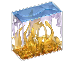
We study the fluid flow occurring in an asymmetric RB rectangular cavity with a rough bottom plate, as sketched in figure 1. The geometrical aspect ratios are set at  $\varGamma _{x}\!=\!W/H\!=\!1$ and $\varGamma _{y}=D/H=0.5$, where $H$ is the height, $D$ the depth and $W$ the width of the cavity. The smooth cold top plate (respectively the hot bottom plate including roughness blocks) is isothermal at constant temperature $T_{S}$ (respectively $T_{R}$). Vertical sidewalls are considered to be adiabatic. No-slip conditions are imposed on walls. The physical problem depends on the Rayleigh number defined as $Ra=\alpha g \Delta T H^{3}/(\nu \kappa )$ and the Prandtl number ( ${Pr}=\nu /\kappa$), where $\alpha$ is the volumetric thermal expansion coefficient, $g$ the gravity, $\Delta T=T_{R}-T_{S}$ the temperature difference, $\nu$ the kinematic viscosity and $\kappa$ the thermal diffusivity. The Prandtl number is taken equal to $4.38$, which corresponds to taking water as the working fluid at a mean temperature of $40\,^{\circ }\textrm {C}$.

Figure 1. (a) Asymmetric RB cavity ( ${R/S}$) with a rough bottom plate. (b) Characteristic lengths of the block spatial arrangement.
The roughness is modelled by a set of square-based blocks. We call the fluid space present between the blocks a valley. The typical size of the blocks (width  $W_{p}$, depth $D_{p}$ and height $H_{p}$) and their horizontal distribution ( $D_{r},W_{r}$) has been chosen to meet two criteria: (i) a roughness height sufficiently large to obtain the first transition between regimes I and II at a Rayleigh number close to $10^{7}$; (ii) a spatial distribution of roughness blocks sufficiently close to Lyon's experiments (Salort et al. Reference Salort, Liot, Rusaouën, Seychelles, Tisserand, Creyssels, Castaing and Chillà2014) to facilitate comparison.
Accordingly, we set the roughness height to  $H_{p}=0.03H$. Following Rusaouën et al. (Reference Rusaouën, Liot, Castaing, Salort and Chillà2018), we estimate the critical Rayleigh number ( $Ra_c$) of the first transition equal to $Ra_{c}=9 \times 10^{6}$ based on an approximation of the thickness of the thermal boundary layer ( $\delta _\theta$) estimated from the Grossmann–Lohse (GL) theory (Stevens et al. Reference Stevens, van der Poel, Grossmann and Lohse2013). The retained shape and distribution of roughness blocks ( $W_{p}=0.075H$, $D_{p}=0.075H$, $H_{p}=0.03H$ and $W_{r}=0.075H$, $D_{r}=0.05H$, see figure 1 for definitions) is equivalent to Lyon's experiment (Salort et al. Reference Salort, Liot, Rusaouën, Seychelles, Tisserand, Creyssels, Castaing and Chillà2014), leading to four rows of six box-shaped blocks to the bottom plate. The resulting ratio between the heat-exchange surface ( $A$) of the asymmetric cavity and that of a fully symmetrical smooth cavity (hereafter respectively denoted as ${R/S}$ and ${S/S}$) is equal to $C_{s}=(A_R+A_S)/(2 A_S)=1.216$. Here, $A_S$ and $A_R$ stand for the dimensionless area of the smooth and the rough plates, respectively, using the cavity height $H$ as length reference, as applied in the following.
2.2. Governing equations and system response
We solve the Navier–Stokes equations under the Boussinesq approximation. Dimensionless equations are written in the following form considering the cell height  $H$ as characteristic length scale, $\Delta T$ as characteristic temperature scale and $({\kappa }/{H})Ra^{0.5}$ as characteristic velocity scale (one obtained from a balance between the friction and buoyancy forces, equivalent to the free-fall velocity divided by $Pr^{0.5}$)
 $$\begin{gather} \boldsymbol{\nabla}\boldsymbol{\cdot}\boldsymbol{u} = 0, \end{gather}$$
 $$\begin{gather}\partial_t \boldsymbol{u}+\boldsymbol{u}\boldsymbol{\cdot} \boldsymbol{\nabla}\boldsymbol{u} ={-} \boldsymbol{\nabla} P^{*}+ {Pr}Ra^{-{1}/{2}} \nabla^{2}\boldsymbol{u}+{Pr} \theta \boldsymbol{e_{z}}, \end{gather}$$
 $$\begin{gather}\partial_t \theta+\boldsymbol{u}\boldsymbol{\cdot}\boldsymbol{\nabla}\theta =Ra^{-{1}/{2}} \nabla^{2} \theta \end{gather}$$
where  $\boldsymbol {u}=(u,v,w)$ is the velocity vector, $t$ the time, $P^{*}$ the dimensionless driving pressure, $\theta$ the temperature and $\boldsymbol {e_{z}}$ the unit vector in the vertical upward direction. The temperature of the top cold plate is taken as reference, so that the dimensionless temperature $\theta$ ranges from $\theta _S=0$ to $\theta _R=1$.
The response of the system to the temperature difference  $\Delta T$ applied to the two horizontal plates is measured in terms of dimensionless heat transfer by the local Nusselt number
 \begin{equation} {Nu(\boldsymbol{x},t)=\sqrt{Ra} \, w(\boldsymbol{x},t) \theta(\boldsymbol{x},t) - \partial_z \theta(\boldsymbol{x},t),} \end{equation}
where  $\boldsymbol {x}=(x,y,z)$ is the coordinate vector. We note by $Nu_{R/S}$, the time and space average of $Nu(\boldsymbol {x},t)$ over the fluid volume contained in the upper part of the asymmetrical RB cavity for $z \ge H_p$. Similarly, $Ra_{R/S}$ refers hereafter to the Rayleigh number imposed on the asymmetric cavity.
Due to the geometrical asymmetry of the configuration, the bulk temperature  $\theta _{bulk}$ is no longer equal to the mean between smooth and rough plates temperatures, i.e. $\theta _{bulk}\neq (\theta _{R}+\theta _{S})/2$. In order to highlight the effect of the asymmetry of the temperature field on each of the horizontal boundary layers (top and bottom), and in particular on the heat fluxes transferred by them respectively, we define two additional temperature differences ( $\Delta \theta _{R}$ and $\Delta \theta _{S}$); $\Delta \theta _{R}$ corresponds to the temperature difference that would be applied to a symmetric RB cavity with a temperature drop at the edges of the boundary layers equivalent to that of the rough half-cavity (bottom) of this study and $\Delta \theta _{S}$ is the same but for the smooth half-cavity (top). Following Tisserand et al. (Reference Tisserand, Creyssels, Gasteuil, Pabiou, Gibert, Castaing and Chillà2011), one can then define two additional Rayleigh and Nusselt numbers related to each plate as follows,
 \begin{equation} \left. \begin{gathered} \Delta \theta_{S} = 2 (\theta_{bulk}-\theta_{S}), \quad \Delta \theta_{R} = 2 (\theta_{R}-\theta_{bulk}),\\ Ra_{S} = Ra_{R/S} \, \Delta \theta_{S}, \quad Ra_{R} = Ra_{R/S} \, \Delta \theta_{R},\\ Nu_{S} = Nu_{R/S} / \Delta \theta_{S} , \quad Nu_{R} = Nu_{R/S} / \Delta \theta_{R}, \end{gathered} \right\} \end{equation}
where we denote by  $Ra_{S}$ (respectively $Ra_{R}$) and $Nu_{S}$ (respectively $Nu_{R}$) the Rayleigh and Nusselt numbers related to the smooth (respectively rough) plate. This is equivalent to taking into account different reference heat fluxes ( $\varPhi _R^{ref}=A_S \Delta \theta _R$ and $\varPhi _S^{ref}= A_S \Delta \theta _S$, here expressed as dimensionless). Note that the issue of different temperature drops within the lower and upper halves of the cavity has also been discussed previously in a context of RB convection under non-Oberbeck–Boussinesq conditions (Weiss et al. Reference Weiss, He, Ahlers, Bodenschatz and Shishkina2018), which do not correspond to the case in the present study.
2.3. Numerical methods and validation
A finite volume approach is applied to discretize the governing equations ((2.1)), by means of the in-house SUNFLUIDH solver. A centred scheme is used for the spatial discretization on a staggered grid and the time discretization is done by a second-order backward differentiation scheme. The diffusive terms are implicitly treated and the convective terms are approximated using the explicit second-order Adams–Bashforth scheme. This leads to a Helmholtz-like equation for each velocity component and the temperature, which is solved by applying the alternating direction implicit method and the Thomas algorithm. The incompressibility constraint is ensured by using a prediction–projection method (Goda Reference Goda1979; Guermond, Minev & Shen Reference Guermond, Minev and Shen2006). The resulting Poisson equation for the pressure is solved by a multi-grid method coupled to the iterative successive over-relaxed algorithm (Strang Reference Strang2007). The flow incompressibility is assessed by calculating the  $L_\infty$ norm of the divergence of the velocity vector, which is kept at around $10^{-9}$. A domain decomposition method is implemented using MPI as well as OpenMP in order to increase the level of parallelism. In this context, the alternating direction implicit method is completed by a Schur decomposition technique. Roughness blocks are not modelled, because we have defined body-fitted meshes. As a consequence, Dirichlet boundary conditions are applied to all walls for velocity and to the top smooth and bottom rough plates for temperature, whereas homogeneous Neumann boundary conditions are applied to all walls for the pressure and to the vertical walls for temperature. SUNFLUIDH code is a general purpose solver for modelling quasi-incompressible fluid flows, such as rotating flows with a free interface (Yang et al. Reference Yang, Delbende, Fraigneau and Martin Witkowski2020), turbulent flows (Derebail Muralidhar et al. Reference Derebail Muralidhar, Podvin, Mathelin and Fraigneau2019) or multi-physics studies (Hireche et al. Reference Hireche, Ramadan, Weisman, Bailliet, Fraigneau, Baltean-Carlès and Daru2020).
Computations are performed for a large range of Rayleigh numbers  $(Ra\in [10^{5}:10^{10}])$ in order to cover the three heat transfer regimes. The initial condition corresponds to the fluid at rest with a uniform temperature ( $\boldsymbol {u} = 0$ and $\theta =0.5$) for all cases, except for the four highest Rayleigh numbers. In these cases, time integration of the governing equations starts from data obtained at the lower Rayleigh number. Statistics sampling begins once the flow regime is settled, which takes between 150 and 300 time units depending on the type of the initial condition and the flow regime. Details about the test cases can be found in table 1. A non-uniform Cartesian grid is constructed for each test case in order to resolve the Kolmogorov microscale ( $\eta$). The mesh size never exceeds $0.55 \eta$ (or $0.76 \eta$) between blocks (or within the cavity bulk, respectively). Moreover, the mesh is refined near the horizontal plates. In particular, up to 56 nodes have been placed along the block height to capture the complex flow inside the valleys. The spatial resolution of the diffusive thermal boundary layer of the smooth top plate meets the criteria proposed by Shishkina et al. (Reference Shishkina, Stevens, Grossmann and Lohse2010).
Table 1. Computational parameters and dimensionless heat transfers:  $Ra_{R/S}$, Rayleigh number imposed to the cavity; $N_{x}\times N_{y}\times N_{z}$, mesh size; $\tau$, time period used for statistics in dimensionless time units; $Nu_{R/S}$, the Nusselt number in the $R/S$ cavity; $(Ra_S, Nu_S)$, the Rayleigh and Nusselt numbers corresponding to the smooth part of the cavity; $(Ra_R, Nu_R)$, and the same for the rough part of the cavity (see (2.3)). $^{\rm a}$ Note that for $Ra \leqslant 2\times 10^{5}$ the flow is stationary.

The space and time convergence of statistics have been verified by computing the global Nusselt number from different formulations as proposed by Stevens, Verzicco & Lohse (Reference Stevens, Verzicco and Lohse2010). This methodology remains applicable for  $z \ge H_p$ due to the adiabatic sidewalls. The obtained values converge with a deviation smaller than $1\,\%$ around the mean value $(Nu_{R/S})$.
The code SUNFLUIDH has been validated in the classic RB configuration beforehand. For this purpose, simulations have been performed in a fully smooth cavity (called  $S/S$) of aspect ratio $\varGamma _y=0.5$ filled with water for Rayleigh numbers up to $Ra=2 \times 10^{9}$, in order to compare with Kaczorowski, Chong & Xia (Reference Kaczorowski, Chong and Xia2014) data. A very good agreement is obtained for the compensated Nusselt number $(NuRa^{-1/3})$, as shown in figure 2.

Figure 2. Compensated Nusselt number as a function of Rayleigh number for the fully smooth cavity ( $S/S$) and the asymmetric cavity ( $R/S$). The blue line corresponds to the Nusselt number increased by the factor $C_s$ (corresponding to the relative increase of the heat-exchange surface in the $(R/S)$ cavity). Red points refer to DNS results from Kaczorowski et al. (Reference Kaczorowski, Chong and Xia2014).
3. Roughness effect on the global heat transfer
3.1. Global heat transfer measured in the asymmetric cavity
The influence of roughness on the heat transfer is first brought to light by comparing the responses of a fully smooth cavity ( $S/S$) and of the asymmetric cavity ( $R/S$). The effect of the roughness on heat transfer due to the increase of the heat-exchange surface area $(C_{s}\times Nu_{S/S})$ is plotted as an indication. Three regimes of heat transfer clearly appear for the $R/S$ cavity in figure 2. (i) A reduction of the Nusselt number $Nu_{R/S}$ compared with $Nu_{S/S}$ is observed at low Rayleigh numbers for one decade in the range $Ra\lesssim 10^{6}$. This phenomenon has already been described experimentally (Tisserand et al. Reference Tisserand, Creyssels, Gasteuil, Pabiou, Gibert, Castaing and Chillà2011) or using two-dimensional simulations (Shishkina & Wagner Reference Shishkina and Wagner2011). (ii) For $Ra \gtrsim 10^{8}$, an increase of the Nusselt number $Nu_{R/S}$ compared with the $S/S$ cavity is obtained, that exceeds the relative increase due to the additional surface due to the roughness blocks as reported in previous works (Tisserand et al. Reference Tisserand, Creyssels, Gasteuil, Pabiou, Gibert, Castaing and Chillà2011). (iii) In between, a transitional regime is present, corresponding to an enhancement of the heat transfer.
The asymmetric cell thus experiences three different heat transfer regimes, two of which correspond to an intensification of the heat transfers compared with a perfectly smooth cell. We now study separately the two smooth top/rough bottom half-cavities of the asymmetric cell ( $R/S$) in the following section.
3.2. Scaling analysis considering each half-cavity individually
We focus on the behaviours of the smooth and rough plates considering the temperature drop of each horizontal boundary layer, as proposed by Tisserand et al. (Reference Tisserand, Creyssels, Gasteuil, Pabiou, Gibert, Castaing and Chillà2011). The results ( $Ra_{S},Nu_{S}$) and ( $Ra_{R},Nu_{R}$) (see (2.3) and table 1) are plotted in figure 3. First, we note that the heat transfer on the smooth plate ( $Nu_S$) follows a single $Nu - Ra$ scaling law. Conversely, the heat transfer on the rough plate $(Nu_R)$ clearly presents two changes in the scaling law. As the regime change is only carried by the heat transfer on the rough wall, we retain the scaling laws for the rough plate ( $Nu_R \sim Ra_R^{\beta }$, given in the caption of figure 3c), to roughly establish the limits of the intermediate regime (around $Ra_R \sim 3\times 10^{6}$ and $1.2\times 10^{8}$). The range of $Ra$ numbers thereby determined will be shaded in all of the figures in the rest of the article. We note that the critical Rayleigh number ( $Ra_c=9 \times 10^{6}$) is in between.

Figure 3. (a) Comparison of the Rayleigh scaling of the Nusselt numbers for the asymmetric  $R/S$ cavity and the smooth $S/S$ cavity and for the rough $R$ and the smooth $S$ plates. (b,c) Compensated Nusselt numbers. The solid lines correspond to the least-squares fits of the $R$ plate results for the three regimes: regime I: $Nu_{R}\sim 0.078 Ra_{R}^{0.34}$, regime II: $Nu_{R}\sim 0.024 Ra_{R}^{0.42}$ and regime III: $Nu_{R}\sim 0.136 Ra_{R}^{0.33}$. The shaded area marks the $Ra$-range of regime II.
As a consequence, three heat transfer regimes can be identified on the rough plate, in agreement with previous experimental studies (Xie & Xia Reference Xie and Xia2017; Rusaouën et al. Reference Rusaouën, Liot, Castaing, Salort and Chillà2018; Tummers & Steunebrink Reference Tummers and Steunebrink2019). In regime I, no difference between the rough and the smooth plates is distinguishable, meaning that the temperature drops viewed by both thermal boundary layers (i.e.  $\Delta \theta _S$ and $\Delta \theta _R$) remain quite similar. In regime III, the rough plate presents a scaling law exponent $\beta$ almost similar to regime I and close to the classic value $1/3$, but the prefactor $\alpha$ is smaller for regime I than for regime III. In contrast, regime II corresponds to an exponent of $\beta \sim 0.42$, indicating an intensified heat transfer.
To summarize, roughness enhances the heat transfer either by increasing the exponent  $\beta$ (regime II) or the prefactor $\alpha$ of the $(Nu-Ra)$ scaling law in regime III for simulations up to $Ra = 10^{10}$. This suggests that regime II can be seen as a transitional regime, after which the flow would revert to a classic organization. However, it is worth noting that, in regime III, the overall heat transfer $Nu_{R/S}$ is larger than the simple additional contribution due to the increase in exchange surface area.
Results obtained in the  $S/S$ cavity have been added to figure 3(b) for comparison with the smooth plate ( $S$). Generally speaking, a similar behaviour (a unique scaling law) is observed for $Nu_{S/S}$ and $Nu_{S}$. This result is consistent with previous experimental observations (Tisserand et al. Reference Tisserand, Creyssels, Gasteuil, Pabiou, Gibert, Castaing and Chillà2011; Wei et al. Reference Wei, Chan, Ni, Zhao and Xia2014). But we note in regime I that the heat transfer is slightly reduced by the addition of roughness in the asymmetric cavity ( $R/S$) when compared with the $S/S$ cavity, as previously shown by Tisserand et al. (Reference Tisserand, Creyssels, Gasteuil, Pabiou, Gibert, Castaing and Chillà2011); Shishkina & Wagner (Reference Shishkina and Wagner2011). An opposite effect is observed in regime III, where $Nu_S$ is slightly larger than $Nu_{S/S}$. A potential interpretation is that, not only the thermal boundary layers are altered by the roughness, but also the dynamics of the bulk flow, as suggested by Wei et al. (Reference Wei, Chan, Ni, Zhao and Xia2014).
3.3. Comparison with experimental data
We seek to assess the relevance of our DNS data with experiments performed in water. The shape of the experimental containers are either cylindrical (Tisserand et al. Reference Tisserand, Creyssels, Gasteuil, Pabiou, Gibert, Castaing and Chillà2011; Wei et al. Reference Wei, Chan, Ni, Zhao and Xia2014; Rusaouën et al. Reference Rusaouën, Liot, Castaing, Salort and Chillà2018) or rectangular (Salort et al. Reference Salort, Liot, Rusaouën, Seychelles, Tisserand, Creyssels, Castaing and Chillà2014). The roughness is made by a set of square box-shaped blocks, except the Wei et al. (Reference Wei, Chan, Ni, Zhao and Xia2014) set-up, where pyramid-shaped blocks are used.
In order to compare the present DNS results with data obtained at Rayleigh numbers three decades higher, a compensated rough Nusselt number is built using a reference value depending on  $Ra$, i.e. the Nusselt number estimated from the GL model $(Nu_{GL})$ using prefactors from Stevens et al. (Reference Stevens, van der Poel, Grossmann and Lohse2013) for a cylinder of aspect ratio $\varGamma =1$. This compensated Nusselt number is plotted as a function of the rough Rayleigh number in figure 4(a). It is shown that all datasets experience similar trends with $Ra$, with a steeper slope from $Nu_R/Nu_{GL} \gtrsim 1$ over one or two $Ra$-decades.

Figure 4. Comparison of the normalized heat transfer on the rough plate with experimental data. Here,  $Nu_{R}$ is normalized by the GL model $(Nu_{GL})$ estimated from Stevens et al. (Reference Stevens, van der Poel, Grossmann and Lohse2013). DNS data are plotted with red open circles ( $\circ$, red). Symbols correspond to experimental data: $H_p=2\ \textrm {mm}$ in the small cavity ( $\vartriangle$, brown; $\vartriangle$, green; $\vartriangle$, blue), or the tall $R/S$ cylindrical cavity ( $\circ$, brown; $\circ$, green) from Tisserand et al. (Reference Tisserand, Creyssels, Gasteuil, Pabiou, Gibert, Castaing and Chillà2011); $H_p=4\ \textrm {mm}$ in the small cavity ( $\blacktriangle$, orange; $\blacktriangle$, green) or the tall $R/S$ cylindrical cavity ( $\bullet$, orange; $\bullet$, green; $\bullet$, blue) from Rusaouën et al. (Reference Rusaouën, Liot, Castaing, Salort and Chillà2018); $H_p = 3\ \textrm {mm}$ $R/S$ (black $\otimes$), $H_p = 8\ \textrm {mm}$ $S/R$ ( $\oplus$, black) and $H_p = 8\ \textrm {mm}$ $R/S$ ( $\ast$, black) in a cylindrical cavity with pyramid-shaped roughness blocks from Wei et al. (Reference Wei, Chan, Ni, Zhao and Xia2014); $H_p=2\ \textrm {mm}$ in a $R/S$ rectangular cavity ( $\Box$, purple; $\Box$, olive; $\Box$, navy) from Salort et al. (Reference Salort, Liot, Rusaouën, Seychelles, Tisserand, Creyssels, Castaing and Chillà2014).
Additionally, Rusaouën et al. (Reference Rusaouën, Liot, Castaing, Salort and Chillà2018) proposed recently to make use of the critical Rayleigh number ( $Ra_c$) to bring out the effect of roughness on the heat transfer, whatever the roughness shape. This is based on the idea that the transition to the enhanced heat transfer regime (II) occurs when the thermal boundary layer thickness $\delta _{\theta }$ becomes of the same size as the roughness blocks. The authors obtained collapsed data, showing the same trend from the reduced heat transfer regime (I) for $Ra_{R}< Ra_{c}$ to an increased regime (III), when applied to experiments performed in asymmetric RB cavities.
The present DNS results agree well with this physical representation. figure 4(b) retains the reduced variables  $(Nu_R/Nu_{GL};Ra_R/Ra_c)$. Normalization by the respective $Ra_{c}$ for each data set allows us to bring together most results, including our numerical data, which fit a similar trend of $Nu$ increase, especially with Lyon's data. In particular, the agreement is remarkable during regime II. This result was hoped for despite a gap of three $Ra$-decades with the experimental configurations, as we use a comparable shape and distribution of roughness blocks. In contrast, a clear decreasing $Nu$ for $Ra_{R}/Ra_{c}\geqslant 10^{2}$ is reported by Wei et al. (Reference Wei, Chan, Ni, Zhao and Xia2014), when using pyramid-shaped roughness. This illustrates the potential influence of the three-dimensional flow dynamics around roughness blocks on the global heat transfer.
4. Contribution of the inner fluid to the heat transfer
The heat transfer regime depends strongly on the pair (Rayleigh number; height of roughness blocks), as shown by the unifying aspect of  $Ra_c$. In the $R/S$ cavity, the vertical heat flux ( $Nu$) below the roughness height is smaller than its global value $(Nu~(z< H_{p})< Nu_{R/S})$ due to the horizontal contribution originating from the vertical surfaces of the roughness blocks. Conversely, $Nu(z\geq H_{p})=Nu_{R/S}$, because of the adiabaticity of the vertical sides of the cavity. For the rough Nusselt number ( $Nu_R$), a similar differentiation between altitudes smaller or larger than the roughness height has to be done; $Nu_R$ results from both the dynamics of the thermal boundary layer above the roughness blocks and the dynamics of the inner fluid retained within roughness valleys. The heat flux measured at $z=H_p$ is an indicator of both dynamics.
In order to gain insights into the mechanisms of heat exchange at the roughness height, we first focus on the rough heat flux  $Nu_{R}$ at $z=H_{p}$, noted hereafter $Nu_R|_{H_p}$; $Nu_R|_{H_p}$ is contributed from two complementary surfaces (see figure 5a): (i) the top surface of the solid blocks, referred to as $Nu_R|^{solid}_{H_p}$, and (ii) the fluid interface between the bulk of the cavity and the inner fluid retained within the roughness valleys, referred to as $Nu_R|^{fluid}_{H_p}$. The heat transfer across the fluid interface at $z=H_p$ $(Nu_R|^{fluid}_{H_p})$ can be divided into two contributions, depending on the heat transfer mode, a conductive part ( $Nu^{cd}_R|^{fluid}_{H_p}$) and convective part ( $Nu^{cv}_R|^{fluid}_{H_p}$). This leads to the following expression:
 \begin{equation} Nu_R|_{H_p}=Nu_R|^{solid}_{H_p}+Nu^{cd}_R|^{fluid}_{H_p}+Nu^{cv}_R|^{fluid}_{H_p} \end{equation}
with
 $$\begin{gather} Nu_R|^{solid}_{H_p}=\dfrac{1}{\Delta \theta_R \, A_S } \int_{A_{solid}} -\partial_z\langle\bar{\theta}\rangle_{A_{solid}} \,\textrm{d}s ; \end{gather}$$
 $$\begin{gather}Nu_R^{cd}|^{fluid}_{H_p}=\dfrac{1}{\Delta \theta_R \, A_S }\int_{A_{fluid}} -\partial_z\langle\bar{\theta}\rangle_{A_{fluid}}\, \textrm{d}s ; \end{gather}$$
 $$\begin{gather}Nu_R^{cv}|^{fluid}_{H_p}=\dfrac{1}{\Delta \theta_R \, A_S }\int_{A_{fluid}} \sqrt{Ra_{R/S}}~\langle\bar{w\theta}\rangle_{A_{fluid}} \,\textrm{d}s, \end{gather}$$
where  $A_{solid}$ ( $A_{fluid}$) is the total area of the top surface of all blocks (of the fluid interface at $z=H_p$ respectively), i.e. $A_S=A_{solid}+A_{fluid}$. The notations $\langle \phi \rangle _{A}$ and $\overline \phi$ stand for the space average over the horizontal surface area $A$ and the time average of the variable $\phi$, respectively.

Figure 5. (a) Sketch of the geometric division of the horizontal plane at  $z=H_p$. (b) Separation of rough heat flux at $z=H_p$ (noted $Nu_{R}|_{H_p}$) into a contribution from the fluid interface $(Nu_{R}|_{H_{p}}^{fluid})$ and from the solid surface $(Nu_{R}|_{H_{p}}^{solid})$. The solid lines correspond to the least-squares fits of the results on the fluid interface for the three regimes: regime I: $Nu_{R}|_{H_{p}}^{fluid}\sim 0.041 Ra_{R}^{0.34}$; regime II: $Nu_{R}|_{H_{p}}^{fluid}\sim 0.005 Ra_{R}^{0.49}$; regime III: $Nu_{R}|_{H_{p}}^{fluid}\sim 0.072 Ra_{R}^{0.34}$. The shaded area marks the $Ra$-range of the regime II.
4.1. Contributions from solid and fluid zones to the rough heat flux
Figure 5(b) compares the evolution of the global rough Nusselt number  $Nu_R$ as a function of $Ra$, with Nusselt numbers originating from the top solid surface of the blocks and from the fluid interface. First, it is shown that the three regimes of heat transfer observed in the $(Ra_R-Nu_R)$ scaling law come mainly from a change of $Nu_R|_{H_p}^{fluid}$. The three power-law fits for $Nu_R|_{H_p}^{fluid}$ are given in the caption of figure 5. In agreement with previous two-dimensional DNS or experiments with pyramid-shaped roughness (see for example Roche et al. Reference Roche, Castaing, Chabaud and Hébral2001; Qiu et al. Reference Qiu, Xia and Tong2005; Toppaladoddi, Succi & Wettlaufer Reference Toppaladoddi, Succi and Wettlaufer2017; Zhu et al. Reference Zhu, Stevens, Verzicco and Lohse2017), we obtain a scaling exponent for regime II close to $1/2$ ( $\beta =0.49$). In contrast, $Nu_R|_{H_p}^{solid}$ is hardly modified by the successive regimes. It can be roughly associated with a single scaling exponent ( $\beta \sim 0.274$, when the data fit is applied to the whole $Ra$-range).
As a consequence, the physical mechanisms responsible for the two transitions between the successive heat transfer regimes appear to be mainly driven by the fluid dynamics occurring within the valleys. This finding is consistent with manipulating the scaling laws of heat transfer through roughness wavelength modification (Toppaladoddi et al. Reference Toppaladoddi, Succi and Wettlaufer2015; Xie & Xia Reference Xie and Xia2017; Zhu et al. Reference Zhu, Stevens, Shishkina, Verzicco and Lohse2019).
4.2. Contributions of conduction and convection to the rough heat flux
The heat transfer through the fluid interface depends both on the temperature field of its conductive part ( $Nu^{cd}_R|^{fluid}_{H_p}$) and on the temperature and velocity fields of its convective part ( $Nu^{cv}_R|^{fluid}_{H_p}$) (see (4.1)). Figure 6(a) illustrates this division. First, we observe that the three successive heat transfer regimes do not appear clearly with $Ra$ increasing in this figure. The critical Rayleigh number $(Ra_c)$ is a significant parameter for the heat transfer through the fluid interface: when $Ra< Ra_c$, the conduction mode is dominant and the convection mode through the fluid interface is negligible, while this is the opposite when $Ra>Ra_c$. A negligible convective heat transfer through the fluid interface does not mean that the fluid within valleys is at rest, but that the mass exchange between the valleys and the bulk is negligible. Around $Ra_c$, the three contributions to $Nu_R$ are of the same order.

Figure 6. (a) Comparison of the different contributions from the solid surface  $(Nu_{R}^{cd}|_{H_{p}}^{solid})$ and the fluid interface ( $Nu_{R}^{cd}|_{H_{p}}^{fluid}$ and $Nu_{R}^{cv}|_{H_{p}}^{fluid}$) to the rough heat flux $Nu_{R}$ at $z=H_{p}$ as a function of the rough Rayleigh number ( $Ra_R$) (see (4.1)). The vertical red line marks the critical Rayleigh number $(Ra_{c})$. (b) Bulk temperature $(\theta _{bulk})$ as a function of $Ra$. The shaded area marks the $Ra$-range of regime II.
Besides, some specific features can be identified in regimes I and III, the intermediate regime II appearing as transitional with the competition between the conductive and convective modes at the fluid interface. In regime I,  $Nu_R|^{solid}_{H_p}$ and $Nu^{cd}_R|^{fluid}_{H_p}$ share a similar trend (in particular the exponent $\beta$ of the scaling law in $Ra$), that is consistent with a diffusive boundary layer covering the top of blocks. In regime III, the dominance of $Nu^{cv}_R|^{fluid}_{H_p}$ on $Nu_R$ reveals an intensification of the mass exchange through the fluid interface. Concurrently, we observe a saturation of the conductive part of the heat transfer through the fluid interface, that forms a plateau around a constant value $(Nu^{cd}_R|^{fluid}_{H_p}\approx 3.7)$. This is also the case for the bulk temperature that saturates around $\theta _{bulk}\sim 0.6$ in regime III in figure 6(b). Moreover, this figure demonstrates the up–down symmetry breaking of the temperature field in regimes II and III.
The dominance of convection and the saturation of  $\theta _{bulk}$ and $Nu^{cd}_R|^{fluid}_{H_p}$ towards constant values suggest that the fluid is well mixed in regime III within the cavity bulk but also within the valleys. As a result, the bottom boundary layer can be assumed to follow the topology of the plate at this regime. Considering uniform diffusive boundary layers of the same thickness covering the top and bottom walls, a simple thermal balance between the top and bottom walls gives an estimate of the bulk temperature as
 \begin{equation} \theta^{*}_{bulk}= \dfrac{A_R \, \theta_R + A_S \, \theta_S}{A_R+A_S}. \end{equation}
The asterisk  $(^{*})$ marks the theoretical estimate of the variable. The above formula gives a good estimate of the bulk temperature ( $\theta ^{*}_{bulk}\simeq 0.59$), when compared with the asymptotic value of figure 6(b). The bulk temperature in regime III is thus only determined by the roughness geometry.
We now explain that this is also the case for  $Nu^{cd}_R|^{fluid}_{H_p}$. At $z=H_p$, we cannot consider that the temperature is equal to $\theta _{bulk}$ due to the inhomogeneity imposed by the alternating of the blocks and the fluid interfaces. A fluid layer at an intermediate temperature ( $\theta ^{*}_i$) results from mixing processes occurring above the roughness height. We refer hereafter to this layer as the fluctuating rough fluid layer.
Additionally, the inner fluid retained inside the valleys can be seen to act as small, well-mixed RB cells with a bulk temperature equal to the mixing temperature of the fluctuating rough layer ( $\theta ^{*}_i$). This enables us to define a film temperature of the inner boundary layer of the valleys, which goes along the bottom wall, as $\theta ^{*}_f=(\theta ^{*}_i+\theta _R)/2$. As a consequence, we can model the conductive heat flux through the fluid interface between the fluctuating rough fluid layer at $\theta ^{*}_{i}$ and the inner boundary layer at $\theta ^{*}_f$, as
 \begin{equation} { Nu^{*cd}_R|^{fluid}_{H_p} = \dfrac{A_{fluid}}{ A_S {\Delta \theta^{*}_R}}\dfrac{ \left(\theta^{*}_f - \theta^{*}_{i}\right)}{H_p}} \quad \text{with} \ \theta^{*}_{i}= \dfrac{A_{fluid}}{A_S} \theta^{*}_{bulk} + \dfrac{A_{solid} }{A_S}\theta_R , \end{equation}
where  $\Delta \theta ^{*}_R$ refers to the estimate of the temperature difference related to the rough half-cavity ( $\Delta \theta ^{*}_R=2 \, ( \theta _R - \theta ^{*}_{bulk}$)). Applying (4.6) to the particular physical configuration of this study, a value of $Nu^{*cd}_R|^{fluid}_{H_p}$ around 4.5 is found for regime III. This is in good agreement with the DNS result. It suggests that, in regime III, the global thermal organization of the cavity is fixed by the geometry, with thermal and velocity boundary layers following the geometry of the roughness and a thicker fluctuating rough fluid layer overlying the roughness, the rest of the cavity being well mixed, including the inner fluid.
5. Effect of roughness on the flow structure
5.1. Boundary layers along the plate centre
In this section, we focus on a restrictive volume of the cavity far from the vertical sidewalls, in order to describe the mean boundary layers developing along the top solid surface of the blocks, or within the valleys and above. To do this, we retain the spatial division methodology of the previous section (in terms of solid or fluid zones), but only considering eight of the 24 blocks located in the centre of the bottom plate, or their direct fluid neighbourhood. Before focusing on the evolution of the boundary layer (BL) thicknesses with the heat transfer regimes, we present the space- and time-averaged vertical profiles of the temperature and horizontal velocity fields close to the top and bottom plates. The horizontal velocity is defined as  $U=\sqrt {u^{2}+v^{2}}$. For clarity reason, we consider three particular $Ra$ belonging to the three regimes, as shown in figures 7 and 8.

Figure 7. Space- and time-averaged vertical temperature profiles in the solid, fluid and smooth zones for three particular  $Ra$: (a) $Ra=2\times 10^{6}$ (regime I); (b) $Ra=5\times 10^{7}$ (regime II); (c) $Ra=10^{9}$ (regime III). The profile for the smooth zone (in green) has been reflected in $(1-z;1-\theta )$ allowing the comparison with rough zone profiles. A profile offset by the distance $H_p$ is plotted for the solid zone with a dashed black line. The red line marks the roughness height $H_p$.

Figure 8. Space- and time-averaged vertical profiles of the horizontal velocity magnitude  $(U=\sqrt {u^{2}+v^{2}})$ in solid, fluid and smooth zones for three particular $Ra$: (a) $Ra=2\times 10^{6}$ (regime I); (b) $Ra=5\times 10^{7}$ (regime II); (c) $Ra=10^{9}$ (regime III). A profile offset by the distance $H_p$ is plotted for the solid zone with a dashed black line. The red line marks the roughness height $H_p$.
As expected, we observe that the thermal BL located along the block top surface and the smooth plate becomes thinner with  $Ra$. But surprisingly, in regimes II and III, the temperature profiles above the blocks and close to the smooth plate appear to be similar in the near wall region, although the bulk temperature value is not equal to the mean temperature of the plates ( $(\theta _S+\theta _R)/2$). The temperature profile in the fluid zone is more complicated. In regime I, a slow decrease of the temperature is observed in the valleys. In regime II, the decrease is more pronounced, but with a change of slope as $z$ passes through $H_p$. This slope change illustrates the onset of the convective heat transfers between the bulk of the cavity and the inner fluid of the valleys. In regime III, the temperature shows a quasi-plateau in the centre of the valleys (see figure 7c), confirming the presence of a kind of secondary well-mixed cells within the valleys. Similar interpretations can be drawn for the viscous BL. In particular, within the valleys, the horizontal velocity increases with the heat transfer regime, up to a plateau in regime III that we can liken to a mean wind (figure 8c).
As seen above, the temperature distribution and the fluid flow within the valleys do not present a classic BL shape. As a consequence, we consider the displacement thickness definition, to take into account inhomogeneity of the temperature and velocity fields, especially within the valleys. The definitions of the thermal and viscous BL thicknesses ( $\delta _\theta$ and $\delta _U$) are as follows,
 $$\begin{gather} \delta_{\theta}=\int_{0}^{0.5}\left(\frac{\langle\bar{\theta}\rangle_A(z)-\theta_{bulk}}{\theta_{R}-\theta_{bulk}}\right)\,\textrm{d}z, \end{gather}$$
 $$\begin{gather}\delta_{U}=\int_{0}^{z_0}\left(1-\frac{\langle\bar{U}\rangle_{A}(z)}{U_0}\right)\,\textrm{d}z \quad \text{with} \end{gather}$$
 $$\begin{gather}U_{0}=max(\langle\bar{U}\rangle_{A}(z): 0 \leq z \leq 0.5) \quad \text{and}\quad z_{0}=z(\langle\bar{U}\rangle_{A}=U_{0}). \end{gather}$$
 The BL thicknesses can be measured over the smooth plate, but also separately above the block top surfaces and the fluid interfaces, following the methodology proposed at the beginning of the present section. Their  $Ra$-dependences are plotted in figure 9. First, we note that a single law (given in the caption of figure 9) is sufficient to describe the $\delta _\theta$ and $\delta _U$ decreases with $Ra$ over the three heat transfer regimes, once the spatial division (solid/fluid) is applied. The similarity between the smooth and solid BL, previously described for three particular $Ra$ in figures 7 and 8, is confirmed. In the fluid zone, the decrease of both BL thicknesses ( $\delta _\theta$ and $\delta _U$) is much slower, although it always remains larger than the BL thicknesses above the solid and smooth zones. However, it is noteworthy that regime II begins with the crossing of $\delta _\theta ^{fluid}$ with $H_p$. This is in good agreement with previous experimental investigations made with different roughness shapes such as Du & Tong (Reference Du and Tong2000) using pyramids, Tisserand et al. (Reference Tisserand, Creyssels, Gasteuil, Pabiou, Gibert, Castaing and Chillà2011); Salort et al. (Reference Salort, Liot, Rusaouën, Seychelles, Tisserand, Creyssels, Castaing and Chillà2014) and Xie & Xia (Reference Xie and Xia2017) using square based parallelepipeds and with the numerical study of Stringano et al. (Reference Stringano, Pascazio and Verzicco2006) using grooved plates. Additionally, we observe that regime II ends when $\delta _U^{fluid}$ becomes smaller than $H_p$, which was also observed experimentally (Xie & Xia Reference Xie and Xia2017).

Figure 9. Displacement boundary layer thicknesses as a function of  $Ra$ and for each space-averaging zone (smooth, solid and fluid). (a) Thermal thickness $\delta _{\theta }$, (b) kinetic thickness $\delta _{U}$. The shaded area illustrates the $Ra$-range of regime II. The red line marks the roughness height ( $H_p$). The black and blue solid lines correspond to the least-squares fits of the results for the solid and fluid zones $\delta _{\theta }^{solid}\sim 0.90 Ra^{-0.25}$, $\delta _{\theta }^{fluid}\sim 0.42 Ra^{-0.17}$, $\delta _{U}^{solid}\sim 0.50 Ra^{-0.21}$, $\delta _{U}^{fluid}\sim 0.28 Ra^{-0.12}$.
A second measure of the BL thicknesses (noted  $\delta ^{rms}$) considers the distance from the wall to the peak of the temperature or horizontal velocity r.m.s.-fluctuations. The figure 10 illustrates their evolution with $Ra$. Once again, we divide the rough cavity part into two parts, the solid zone above the roughness blocks and the fluid zone above the valleys. As already observed, the smooth and solid $\delta _\theta ^{rms}$ and $\delta _U^{rms}$ follow a similar trend, with a single scaling law describing the BL thickness decrease whatever the regime. We note that the thermal BL along the smooth wall remains always slightly thicker than the solid one above the roughness blocks. The fluid BL behaves in a different way. After becoming thinner with $Ra$ in regimes I and II, $\delta _\theta ^{rms}$ and $\delta _U^{rms}$ tend towards a plateau in regime III, that corresponds approximately to the roughness height. This plateau can be interpreted as the signature of a fluctuating rough fluid layer mentioned in § 4.2. Moreover, for this regime and the fluid region, a second local maximum can be determined in the vertical profiles of temperature and velocity field r.m.s.-fluctuations, that defines a turbulent BL within valleys of a similar thickness to $\delta _\theta ^{rms}$ and $\delta _U^{rms}$ for the solid region and the smooth plate. It confirms the onset of a turbulent RB convection-like flow within valleys in regime III.

Figure 10. The root-mean-square (r.m.s.) based boundary layer thicknesses as a function of  $Ra$ and for each space-averaging zone (smooth, solid and fluid). See (5.1) and (5.2) for definitions. (a) Thermal boundary layer thickness $\delta _{\theta }^{rms}$ measured as the peak of $\theta _{rms}$; (b) kinetic BL thickness measured as the peak of $U_{rms}$. The shaded area illustrates the $Ra$-range of regime II. The red line marks the roughness height ( $H_p$).
5.2. Global flow structure
The effect of roughness on the flow structure is first investigated by considering temperature fluctuations around the roughness (see figure 11). We observe that a turbulent layer develops around the roughness in all cases. However, while in regime I this layer remains mainly above the roughness, it fills almost entirely the valleys in regime II. In regime III, a less fluctuating small flow takes place within the valleys, with a BL along the bottom plate and a turbulent layer around  $z\sim H_p$, illustrating interactions between the valley flow and the large-scale circulation (LSC). These two layers are responsible of the two peaks observed in the r.m.s.-fluctuations used to define the BL thicknesses displayed in figure 10. Additionally, it is noticeable that the temperature fluctuations are particularly intense in regime II, when compared with regimes I and III.

Figure 11. Temperature fluctuation r.m.s. field ( $\theta _{rms}$) on vertical planes in the vicinity of the rough plate for three particular $Ra$: (a,d) $Ra=2\times 10^{6}$ (regime I); (b,e) $Ra=5\times 10^{7}$ (regime II); (c,f) $Ra=10^{9}$ (regime III). (a–c) Above a row of roughness blocks ( $y=0.3125$); (d–f) between two rows of roughness blocks ( $y=0.25$). The $x$-axes of (b,e) have been flipped to maintain a similar direction of large-scale circulation for all Rayleigh numbers.
Figure 12 illustrates how the change in the heat transfer regime modifies plume organization. A qualitative overview of the isocontours of instantaneous temperature shows a number of large hot plumes within the cavity bulk in regime II (figure 12b), while plumes appear more altered by the LSC in regime III (figure 12c,d). Moreover, asymmetry of the flow seems to appear for regimes II and III.

Figure 12. Instantaneous temperature field for (a)  $Ra=2\times 10^{6}$ (regime I), (b) $Ra=5\times 10^{7}$ (regime II), (c) $Ra=10^{9}$ (regime III) and (d) $Ra=10^{10}$ (regime III). Isosurface values correspond to $\theta =(0.2,0.45,0.65,0.8)$.
A more global point of view can be obtained by considering the spatial average of the r.m.s. temperature over the volume of half a cavity  $(V = V_R \textrm { or } V_S)$, as a function of $Ra$. As plotted in figure 13(a), the asymmetry of temperature r.m.s.-fluctuations only occurs in regime II, where larger values are present on the rough part of the cavity rather than on the smooth part. But for each half-cavity, the maximum value of fluctuations is reached around $Ra_{c}$. Unlike regime II, the intensity of $\theta _{rms}$ is similar on both parts of the cavity in regimes I and III. These observations are in agreement with the statement of Du & Tong (Reference Du and Tong1998), that interactions between roughness and LSC enhances the detachment of the thermal BL leading to extra thermal plumes, but only in regime II in our case.

Figure 13. (a) Integral of r.m.s. temperature fields over the fluid volume in half a cavity ( $V_R$ volume of the rough half-cavity; $V_S$ volume of the smooth half-cavity). The vertical red line represents the critical Rayleigh number $Ra_{c}$. (b) Friction coefficient normalized by dissipation vs Reynolds number. The dashed lines display $Re_U^{-0.5}$ power laws. Inset: the Reynolds number $Re_U$ as a function of the Rayleigh number $Ra$ for the two half-cavities. Data for the rough part can be fitted by a power law: $Re_R=0.054 Ra_R^{0.48}$ (regime I), $Re_R=0.009 Ra_R^{0.58}$ (regime II) and $Re_R=0.029 Ra_R^{0.53}$ (regime III). The shaded area illustrates the $Ra$-range of regime II.
Mechanical interactions of the LSC with roughness can be quantified considering the Reynolds number ( $Re_U$) based on the maximum of the horizontal velocity ( $\left \langle \bar {U} \right \rangle$). In a similar manner as $Nu$ and $Ra$,
$Ra$,  $Re_U$ can be estimated separately for the rough or smooth parts of the cavity. Figure 13(b) (inset) presents its evolution as a function of $Ra$. The scaling laws are given in the caption for the rough part of the cavity. It can be noted that no clear difference between the two half-cavities is noticeable, except for regime III, where the LSC appears to be stronger in the rough part than in the smooth part. This suggests that the increase in the $\alpha$ prefactor of the scaling law ( $Nu_R - Ra_R$) observed in regime III, could result from a faster LSC, since the temperature fluctuations remain similar in the two half-cavities. Moreover, the scaling exponents of $Re_U$ ( $\beta _R=0.58$) and $Nu_R$ ( $\beta _R=0.42$) with $Ra_R$ obtained for regime II are consistent with the regime IIIu proposed by the GL theory (Grossmann & Lohse Reference Grossmann and Lohse2000, Reference Grossmann and Lohse2001). This means that the bulk contribution to the thermal dissipation rate is dominant (here, the heat is injected directly by the roughness within the bulk), while the BL contribution remains dominant for the energy dissipation rate.
From the above dimensionless numbers, a friction coefficient can be built as  $Nu Ra / (Re_U^{3} Pr^{2})$ (Chavanne et al. Reference Chavanne, Chillà, Chabaud, Castaing and Hébral2001) for each side of the cavity separately. This is equivalent to the ratio $\epsilon _u/\epsilon _{u,bulk}$, where $\epsilon _u$ is the global energy dissipation rate, and $\epsilon _{u,bulk}$ its bulk contribution. Given the exact relation $\epsilon _u=({\nu ^{3}}/{H^{4}})(Nu-1)Ra Pr^{-2}$ (Siggia Reference Siggia1994) and the $Re$ dependences of the bulk and the BL contributions ( $\epsilon _{u,bulk}\sim Re^{3}$ and $\epsilon _{u,BL}\sim Re^{5/2}$), the friction coefficient is expected to vary with $1/\sqrt {Re}$ when the total energy dissipation is dominated by the laminar velocity BLs (Chavanne et al. Reference Chavanne, Chillà, Castaing, Hébral, Chabaud and Chaussy1997). In figure 13(b), the friction coefficient vs $Re_U$ is displayed. As observed for $Re_U$, both sides of the cavity evolve in a similar way. Unsurprisingly, it is seen that the friction coefficient fits quite well with the $Re^{-1/2}$ power law, as already observed by Chavanne et al. (Reference Chavanne, Chillà, Chabaud, Castaing and Hébral2001) for $Re$ lower than $10^{4}$. In our study, the velocity BLs are therefore laminar whatever the regime. Interestingly, the friction coefficient is higher during regime II compared with regimes I and III. This can be interpreted as stronger interactions between the flow coming from the roughness region and the LSC, when the block top is sandwiched between the thermal and kinetic BL ( $\delta _\theta \leq H_p \leq \delta _U$).
6. Conclusion
In this paper, we present DNS results of turbulent RB convection in an asymmetric rough water-filled cavity for five decades in Rayleigh number ( $Ra\in [10^{5}-10^{10}]$). The study case has been dimensioned in order to obtain a moderate value of the critical roughness-height-based Rayleigh number ( $Ra_c=9\times 10^{6}$). The resulting rough plate consists of a sufficient number of box-shaped blocks to consider that the influence of the flow along the vertical walls is negligible in the central part of the cavity. The main objective of this study is to determine whether particular physical mechanisms in the block surroundings can explain the enhanced heat transfer in regimes II and III. For this purpose, it is proposed to use a single physical set-up to capture the two successive heat transfer regime transitions.
First, a global description of the heat transfer in the asymmetric cavity  $R/S$ is discussed. As expected, we have identified three successive regimes of heat transfer: (i) a thermally resistant regime I where the global Nusselt number ( $Nu_{R/S}$) is reduced compared with the heat transfer in a perfectly smooth cavity ( $Nu_{S/S}$), (ii) a transitional regime II where the heat transfer is particularly intense and (iii) a regime III in which the increase of $Nu_{R/S}$ is larger than the relative increase of surface due to roughness. By considering the typical temperature drops of each horizontal BL, individual Rayleigh and Nusselt numbers have been constructed for each plate. It is seen that only one scaling exponent describes the heat transfer on the smooth plate, whereas two scaling exponents stand for the rough plate ( $Nu_R\sim Ra^{\beta }_R$): in regimes I and III, $\beta _{R}\sim 1/3$ is found and it increases to $\beta _{R}=0.42$ in regime II. Based on the parameters of the rough plate ( $Ra_R, Nu_R$), the relevance of the DNS results has been assessed regarding experimental data from the literature, despite a gap of three $Ra$-decades with the experiments.
In order to highlight the role of the inner fluid retained within roughness valleys, the horizontal plane at the roughness height is divided into two parts, which enables us to define two distinct heat transfer contributions: a first one coming from the solid top surface of the roughness blocks, and a second one passing through the fluid interface between the cavity bulk and the inner fluid. Whatever the heat transfer regime, a unique scaling law holds for the heat transfer on the solid top surface. In contrast, the fluid interface at  $z=H_p$ appears to fully drive heat transfer in the rough half-cavity. Concerning $Nu_R|^{fluid}_{H_p}$, the $\beta$ exponent of the $(Nu-Ra)$ scaling law is approximately $\beta _{F}\sim 1/3$ in regimes I and III and it increases to $\beta _{F}\sim 0.5$ in regime II, which agrees well with experimental results obtained with pyramid-shaped roughness elements.
By using the decomposition of the rough Nusselt number at the fluid interface ( $Nu_R|^{fluid}_{H_p}$) into conductive and convective parts, it has been shown that conduction is the dominant mode of heat transfer from the valleys to the bulk in regime I. Convection contribution becomes sufficiently large in regime II to compete against conduction. In regime III, convection becomes the dominant mode, while heat transfer by conduction saturates at a specific value. This value, as well as the bulk temperature, is shown to depend only on geometric parameters. It suggests that the flow in regime III is organized in the form of BLs flowing along the geometry of the top and bottom plates and of a separate fluctuating rough fluid layer overlaying roughness. The fluid volume can be considered to be well mixed, including the small fluid volumes within the roughness valleys.
Since the heat transfer is initiated inside the BLs, the  $Ra$-evolution of their thicknesses has been analysed by adopting the previous spatial division (viz. smooth plate/the solid zone above the top surface of blocks/the fluid zone located inside the valleys and above). Considering the displacement BL thicknesses, only the BLs within valleys mark out the limits of regime II. As proposed by Xie & Xia (Reference Xie and Xia2017) for $Pr$ larger than 1, it is observed that this regime starts when the thermal BL is thinner than the roughness height and ends when the kinetic BL is thinner than the roughness height. Concurrently, the BL above blocks behaves like a smooth BL, becoming thinner than the roughness height early in regime I.
A measure of the fluctuating rough fluid layer thickness has been obtained by tracking the peaks of the temperature r.m.s.-fluctuations. This measure points out the presence of this fluid layer only in regime III.
Finally, a global point of view is adopted. It is shown that the top and bottom half-cavities display the same level of thermal fluctuations, except in regime II where more intense fluctuations are present in the rough part. This is in agreement with the Du & Tong (Reference Du and Tong1998) interpretation of extra plumes emissions by roughness, but only for regime II. Using a Reynolds number based on the maximum of the time-averaged horizontal velocity, the friction coefficient is calculated. It follows a  $Re^{-1/2}$ power law, suggesting a laminar velocity BL whatever the regime, but with a higher prefactor for regime II. The LSC and the flow coming from the roughness region therefore interact more strongly. Moreover, the $Ra_R$ dependence in regime II of both $Re_R$ and $Nu_R$ present scaling exponents ( $\beta _R=0.58$ and 0.42, respectively) consistent with the regime IIIu proposed by the GL theory (Grossmann & Lohse Reference Grossmann and Lohse2000, Reference Grossmann and Lohse2001), meaning that the bulk contribution to the thermal dissipation rate is dominant, while the BL contribution remains dominant for the energy dissipation rate. In regime III, the Reynolds number of the rough half-cavity becomes higher than in the smooth one. The increase in the heat transfer scaling prefactor ( $\alpha _R$) observed at this regime could result from a faster and more efficient LSC in transporting heat, as the temperature fluctuations remain similar in both half-cavities.
However, these conclusions pertain to a particular Prandtl number and a range of moderate Rayleigh numbers due to the value of the set critical Rayleigh number. Further investigations should be performed to clarify the interplays between roughness, LSC and a higher turbulence level.
Acknowledgements
We are grateful to F. Chillà and J. Salort for valuable discussions.
Funding
This study was granted access to the HPC resources of GENCI-IDRIS under allocation 2a0326 made by GENCI. This work has benefited from the financial support of the INSIS CNRS (PEPS Energie 2018).
Declaration of interests
The authors report no conflict of interest.


 Open access