


1. Introduction
Some months ago, an article (Kuehnen et al. Reference Kuehnen, Song, Scarselli, Budanur, Riedl, Willis, Avila and Hof2018b) was brought to our attention about a set of extraordinary experiments that could turn a turbulent flow into laminar before your eyes, without reducing its bulk velocity. All experiments begin with a steady-state fully developed turbulent pipe flow, which is disturbed by different agents until it finally turns into a laminar Hagen–Poiseuille flow downstream. The bulk velocity (Reynolds number) is kept strictly constant during each process. In the first experiment, the disturbance is caused by four small electric rotors inserted within the flow, which can be switched on and off. While they are static, the flow is turbulent. Upon powering them, they stir the fluid around vigorously and the flow becomes laminar farther downstream. In the second, a previously diverted portion of the fluid is reinserted into the flow through a set of 25 thin holes drilled helically in the pipe's wall, creating 25 identical small radial jets that disrupt the flow circulating within the pipe. The flow is initially turbulent with the jets switched off and, again, upon starting the jets, the flow turns laminar farther downstream. In the third experiment, a short segment of pipe is replaced by a device that has a circular narrow gap parallel to the pipe's wall. Again, a previously diverted portion of the fluid is reinserted into the flow through the gap, creating an annular streamwise jet next to the wall and, once more, the perturbed flow becomes laminar farther downstream. In the last experiment, a long segment of pipe is replaced by a slightly thicker one that can slide streamwise rather rapidly. While the segment is static, the flow is turbulent, whereas after sliding at velocities slightly above the flow's bulk velocity, a laminar flow is recorded downstream. We strongly recommend reading Kuehnen et al. (Reference Kuehnen, Song, Scarselli, Budanur, Riedl, Willis, Avila and Hof2018b) before continuing with this paper, since a previous knowledge of its content is assumed.
A few years ago, we finally solved the Reynolds-averaged Navier–Stokes equation (RANSE) for any fully developed incompressible pipe flow (García García Reference García García2017; García García & Fariñas Alvariño Reference García García and Fariñas Alvariño2019b), a second-order parabolic partial differential equation on the mean-velocity field. The general solution takes the form of a Fourier–Bessel series, rooted in a weighted Hilbert space  $L^2_{\alpha }(0,1)$, which is the functional space where the ensemble-averaged flow fields are defined. With this solution we can obtain the mean-velocity field of any flow, regardless of its being laminar, turbulent, steady or unsteady, always provided that it is fully developed. Using the said general solution as a cornerstone, we have built a theory that explains and predicts an ever-growing number of features and properties of pipe flows, some of them radically new. It is known as the theory of underlying laminar flow (TULF), for reasons that will become clear shortly, and we have already applied it to successfully explain unsteady flows (U-flows) reported in the literature (García García & Fariñas Alvariño Reference García García and Fariñas Alvariño2019c, Reference García García and Fariñas Alvariño2020, Reference García García and Fariñas Alvariño2021), some of which have remained unexplained for decades.
The TULF is a theory of mean flows; it is not a theory about physical flows. Physical flows (realisations) respond to the Navier–Stokes equations, which are nonlinear, and are subject to turbulent streaks, coherent structures, nonlinearities, chaos and show an extreme variability, whereas mean flows (ensemble average of infinite realisations) respond to the RANSE, which in the case of pipe flow is a perfectly linear differential equation, and does not show any of the nonlinearities mentioned above. The linear superposition principle holds in the RANSE for pipe flow (and other canonical flows) and we make good use of it. This is the main reason why the RANSE has been solved for some canonical flows, while the corresponding Navier–Stokes equations still await solution. What it is hard to explain is why the general solution of the RANSE for those canonical flows had to wait almost a century and a half, until it finally came from Spain. Even harder if one acknowledges the particular solution for pipe steady flow (S-flow) offered in Pai (Reference Pai1953), which should have triggered the quest for the general solution of any mean pipe flow.
A mean flow only shows streaks or other turbulent structures if they are repeatable enough to be present in all realisations, at about the same position and time. A mean flow cannot be physical, and vice versa, except in the case of purely laminar flow. Mathematically: a turbulent mean flow is not a solution of the Navier–Stokes equations and a turbulent physical flow is not a solution of the RANSE. Later, we shall see that solutions of the RANSE belong to a functional space that is essentially different from physical space.
Since the four experiments destabilising turbulence described above qualify as pipe flow, it is to be expected that the TULF could also furnish an explication to them, for they may stand to reason. The present research aims to grant a detailed explanation of the process and mechanism whereby the turbulence vanishes from a turbulent flow. The account we shall offer is of a physico-mathematical character, based entirely upon the TULF, albeit we shall employ a very simple model, lest the description be marred by complicated mathematics. We shall see that even a simple model suffices to illustrate the behaviour leading to the flow's laminarisation. And most important, the model will allow us to calculate the new pressure gradient that must be enforced in a flow to laminarise it completely. After learning how (and how much) things happen, we expect researchers to be successful in designing new insightful ways to remove turbulence from pipe flows.
Possibly, this is the right place to praise the ingenuity demonstrated by the authors of those experiments, which are so extraordinarily suited to test our theory that we cannot think of any better set of proofs for it. We, despite having the decisive advantage of knowledge, would have been unable to design them ourselves, let alone to craft them with such care and quality.
Of the four experiments, rotors, radial jets, annular streamwise jet and sliding pipe segment, the first three respond to a common pattern for laminarisation, whereas the fourth involves a considerably more complex mechanism, in which the sliding-wall velocity enters into the mathematical equations. Since explaining the laminarisation under a sliding pipe segment is rather lengthy, and this paper is already long enough, we have decided to relay the account of this phenomenon to a future publication, and thereby it will not be considered any further in the remainder of this one.
In order to fully understand the coming explanations, a certain knowledge of the TULF scope and methods would be necessary. Therefore, we shall begin this work with some basic notions, albeit a comprehensive account can be found in our previous publications (García García & Fariñas Alvariño Reference García García and Fariñas Alvariño2019b,Reference García García and Fariñas Alvariñoc, Reference García García and Fariñas Alvariño2020, Reference García García and Fariñas Alvariño2021). The TULF is a theory heavily based upon mathematical analysis, and most of the concepts that will be introduced, however strange they might appear at first sight, arise out of mathematical necessity. Thus, only the hypothesis leading to some results or the physical interpretation of them would be subject to discussion, although not the results themselves.
This article is structured as follows. We begin with a brief account of the proposed formalism, where we shall learn the basic notions of the TULF without which hardly any explanation would be feasible. This introductory part ends with the most comprehensive solution to the governing equation of fully developed mean pipe flow that, to our knowledge, has ever been proposed. Then, we use the information gained to build a general schematic sequence of the laminarisation process, which is applicable to the three experiments of (Kuehnen et al. Reference Kuehnen, Song, Scarselli, Budanur, Riedl, Willis, Avila and Hof2018b), and with such a laminarisation pattern we proceed to explain them. Next, we take the general solution to devise the simple mathematical model referred to above. The model yields to some equations that are applied to each experiment, producing numerical data that are contrasted with the experimental results. Also, a figure of merit is proposed to assess the effectiveness of each laminarisation method. Finally, we end this work with a summary of our conclusions and an address to researchers willing to design experiments in which turbulence vanishes.
In this paper, whenever we say ‘flow’ it should be understood as ‘fully developed flow’, unless otherwise specified. Henceforth, the terms U-profile, U-field, U-flow, U-configuration, etc. will be used to denote the unsteady profile of any quantity, or any characteristic of unsteady flows; whereas the terms S-profile, S-field, S-flow, S-configuration, etc. will refer to the corresponding statistically steady-state profile or characteristic. A list of all acronyms used can be found in Appendix A. The present article is the fifth in a series (García García & Fariñas Alvariño Reference García García and Fariñas Alvariño2019b,Reference García García and Fariñas Alvariñoc, Reference García García and Fariñas Alvariño2020, Reference García García and Fariñas Alvariño2021) that intends to explain a number of experimental results reported in the literature, which to date remain unexplained.
2. Laminar Hagen–Poiseuille pipe flow
Most concepts presented in this section are already well known, but they need be repeated so that we can cogently link the ideas leading to the object of this article. The physical system under study is an inclined pipe of diameter  $D=2R$ and indefinite length, filled with a Newtonian incompressible fluid of constant density $\rho$ and kinematic viscosity $\nu$ (see figure 1 with $V_w=0$). A cylindrical coordinate system $(r,\theta,z)$ is naturally defined in the pipe, whose centreline is taken as the $z$-axis. The fluid is driven by the combined action of a pressure gradient $G=-\mathrm {d} p / \mathrm {d} z \geq 0$, constant in time, and the gravity force density $-\rho g \cos \varTheta$, both causing a steady-state flow with velocity field $\boldsymbol {u}=[u_i]=[u_r,u_{\theta },u_z]$. The influence of gravity across the pipe section is neglected and only its effect along the streamwise direction is contemplated. Circular symmetry is assumed within the pipe, thereby $u_{\theta }=0$ and $\partial u_i/\partial \theta =0$ for any component $u_i$. Only fully developed flow is considered, which implies $\partial u_i /\partial z =0$ . In these conditions, it can be proved (White Reference White2016, § 4.10) that the flow is one-dimensional, parallel to the pipe axis, the velocity field only depends upon $r$ (
$r$ ( $\boldsymbol {u}=[0,0,u_z(r)]$) and the pressure gradient is also constant in space. The governing equation for steady-state laminar pipe flow is the one-dimensional Navier–Stokes equation (see White Reference White2016, p. 265)
 \begin{equation} \frac{\mathrm{d}^2 u_z}{\mathrm{d} r^2} + \frac{1}{r} \frac{\mathrm{d} u_z}{\mathrm{d} r} ={-}\frac{G}{\rho \nu}-\frac{g \cos \varTheta}{\nu}, \end{equation}
subject to the no-slip boundary condition,  $u_z(R)=0$, whose solution is the well known Hagen–Poiseuille flow,
 \begin{equation} u_z(r)=\frac{(G+\rho g \cos \varTheta) R^2}{4 \rho \nu} \left( 1-\frac{r^2}{R^2} \right). \end{equation}
In (2.1),  $G+\rho g \cos \varTheta$ acts as the cause of the fluid's motion, i.e. as the source of the field $u_z(r)$. It is very convenient to express our results in dimensionless form. We shall define the natural normalisation, in which the dimensionless variables and fields are expressed as
 $$\begin{gather} \alpha=\frac rR, \quad \beta=\frac zR, \quad \tau=\frac{t\nu}{R^2}, \end{gather}$$
 $$\begin{gather}u(\alpha)= \frac{u_z(r) R}{\nu}, \quad \mathfrak{p}=\frac{(p-p_0) R^2}{\rho \nu^2}, \quad \sigma_w=\frac{\tau_w R^2}{\rho \nu^2}, \quad \varPi=\frac{G R^3}{\rho \nu^2}, \quad \varGamma=\frac{g R^3 \cos \varTheta}{\nu^2}, \end{gather}$$
where  $p_0$ is a reference pressure at $r=R$ and $z=0$, and $\tau _w$ the wall-shear stress (WSS). In the natural normalisation, (2.2) adopts the simple form
 \begin{equation} u(\alpha)=\frac{\varPi+\varGamma}{4}(1-\alpha^2), \end{equation}
which is also known as the Hagen–Poiseuille parabola. The mathematical details for deriving equations in the natural normalisation are found in García García & Fariñas Alvariño (Reference García García and Fariñas Alvariño2019b).

Figure 1. Schematics of general pipe flow.
In pipe flow we can also define the dimensionless quantities, WSS ( $\sigma _w$), friction velocity ( $u_{\tau }$), cross-section-averaged or bulk velocity ( $\tilde {u}$), Darcy friction factor ( $f$), skin-friction coefficient ( $C_f$), as follows:
 $$\begin{gather} \sigma_w = \frac{\mathrm{d} u(1)}{\mathrm{d} \alpha} , \quad u_{\tau}=\sqrt{|\sigma_w|} , \quad \tilde{u}=2\int_0^1 \alpha u(\alpha) \, \mathrm{d} \alpha, \end{gather}$$
 $$\begin{gather}f=\frac{4( \varPi+\varGamma)}{\tilde{u}^2} , \quad C_f=\frac{2|\sigma_w|}{\tilde{u}^2}=2 \left( \frac{u_{\tau}}{\tilde{u}} \right)^2, \end{gather}$$
and also the Reynolds number,  $Re=\widetilde {u_z} D /\nu$. These quantities are positive real numbers, except the WSS which is negative because it opposes motion. We adopt a sign convention that establishes $\sigma _w= -( \varPi +\varGamma )/2$ for Hagen–Poiseuille flow. Among all dimensionless quantities defining this laminar S-flow, we can establish the following simple relationship (see White Reference White2016):
 \begin{equation} Re = 2\tilde{u} = u(0) = \frac{\varPi+\varGamma}{4}={-} \frac{\sigma_w}{2} = \frac{u_{\tau}^2}{2} = \frac{64}{f}=\frac{16}{C_f}, \end{equation}
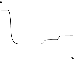
whereby given any one of them, the remaining become automatically fixed, and possibly the easiest to measure in a flow is  $\varPi +\varGamma$. Equation (2.8) is decisive for the present research and we shall call it the zero theorem of laminar fully developed steady-state Hagen–Poiseuille pipe flow, or simply laminar Hagen–Poiseuille flow. Note the zero theorem is a rigorous mathematical statement, not a rule of thumb. Also, from the zero theorem follows the very compact and neat expression for the velocity field,
 \begin{equation} u(\alpha)=Re (1-\alpha^2), \end{equation}
valid only for laminar S-flow. Equations (2.8) and (2.9) illustrate how a convenient choice of reference units, such as the natural normalisation introduced herein, contributes to simplify the expressions of a science, which now adopt a very elegant form.
3. Turbulent Hagen–Poiseuille pipe flow
Turbulent flows are normally approached from a different standpoint. As the physical fields are so fluctuating, knowing the instantaneous flow is both difficult and less interesting; instead, it is preferred to determine the average fields and there are various averaging methods (see García García Reference García García2017, § 3.2), being the ensemble average over an infinite number of realisations that is chosen herein. With this approach, the velocity field in S-flow would be expressed as  $\boldsymbol {u}(t,\boldsymbol {x})=\langle \boldsymbol {u}(\boldsymbol {x}) \rangle +\boldsymbol {u}'(t,\boldsymbol {x}) \equiv \boldsymbol {U}(\boldsymbol {x})+\boldsymbol {u}'(t,\boldsymbol {x})$, whereby $\boldsymbol {u}(t,\boldsymbol {x})$ is the time-dependent instantaneous physical field, $\langle \boldsymbol {u}(\boldsymbol {x}) \rangle \equiv {\boldsymbol{U}}(\boldsymbol {x})$ is the time-constant average or mean field and $\boldsymbol {u}'(t,\boldsymbol {x})$ is simply the difference between the two, called the fluctuating component. A similar decomposition can be performed for any other flow field: pressure, temperature, vorticity, etc. Note that mean fields are not physical fields, meaning that not a single realisation of the actual flow would yield a set of values equal to those of the mean field; in mathematical terms, the set of space–time points at which $\boldsymbol {u}'(t,\boldsymbol {x})=0$ has measure zero, i.e. is a null set. Mean fields are mathematical entities that belong to, shall we say, the mean space, which is not the physical spacetime. To fix ideas, we shall denote with $\mathfrak {M}$ the set of mean fields arising in fully developed pipe flow; we shall see later, in § 5, that the mean space is actually a subset of the weighted Hilbert space $L^2_{\alpha }(0,1)$, $\mathfrak {M} \subset L^2_{\alpha }(0,1)$. Of course, in the case of a strictly laminar flow, mean fields and instantaneous physical fields are coincident.
The governing equation for the mean-velocity field is not the Navier–Stokes equation, but rather the RANSE. The RANSE is almost formally identical to the Navier–Stokes equation: an extra term must be added including the so-called Reynolds stresses  $\langle \rho u'_i u_j' \rangle$. In the case of turbulent fully developed statistically steady-state Hagen–Poiseuille mean pipe flow (see figure 1 with $V_w=0$), or simply turbulent Hagen–Poiseuille flow, the only component of interest for this section is the time-constant Reynolds shear stress (RSS) $\langle \rho u'_r u_z' \rangle (\boldsymbol {x})$, whose dimensionless version in the natural normalisation is given by
 \begin{equation} \sigma(\alpha) = \frac{\langle \rho u'_r u_z' \rangle R^2 }{\rho \nu^2}. \end{equation}
The mean flow, which only exists in the mean space  $\mathfrak {M}$, is determined by the combined action of the mean pressure gradient (MPG), gravity and RSS. The physical velocity field of any particular realisation, $\boldsymbol {u}(t,\boldsymbol {x})$, does not ‘feel’ the Reynolds stress: each individual flow is exclusively driven by actual pressure gradient, gravity and viscous forces. Only upon averaging does the notion of Reynolds stress emerge, and averaging is a mathematical operation, not a physical one. One of the most paradoxical facts of turbulent flows is that the mean-velocity field is not a solution of the Navier–Stokes equation, and vice versa, the physical instantaneous velocity field cannot be a solution of the RANSE. Mean and physical fields are disjoint sets in turbulent flows; we shall never see any mean turbulent flow occurring in laboratory. In computational fluid dynamics terms, even if the Reynolds stresses were perfectly modelled, a perfect Reynolds-averaged simulation cannot yield the same results as one perfect direct numerical simulation (DNS), for the equations solved are different.
The dimensionless mean-velocity field is also denoted by  $u(\alpha )$, since laminar flow would be the particular case of mean flow with $\sigma (\alpha )=0$. Taking into account the RSS, the RANSE is expressed as
 \begin{equation} \frac{\mathrm{d}^2 u}{\mathrm{d} \alpha^2} + \frac{1}{\alpha} \frac{\mathrm{d} u}{\mathrm{d} \alpha} ={-}\varPi-\varGamma+\frac{1}{\alpha}\frac{\mathrm{d}(\alpha \sigma)}{\mathrm{d} \alpha}={-}\varPi-\varGamma-\varSigma(\alpha) , \quad \alpha \in (0,1), \ u,\sigma,\varSigma \in \mathfrak{M}, \end{equation}
together with the no-slip boundary condition  $u(1)=0$, the symmetry boundary condition $\mathrm {d} u(0)/\mathrm {d} \alpha =0$ and boundary conditions for the RSS, $\sigma (0)=\sigma (1)=0$. The field $\varSigma (\alpha )=-(1/\alpha )\mathrm {d}(\alpha \sigma )/\mathrm {d} \alpha$ is the RSS radial gradient (RSSRG). The solution of (3.2) in the natural normalisation is (Pai Reference Pai1953)
 \begin{equation} u(\alpha)=\frac{\varPi+\varGamma}{4}(1-\alpha^2)-\int _{\alpha}^{1} \sigma(\alpha') \, \mathrm{d} \alpha' , \quad \sigma(\alpha)=\frac{\mathrm{d} u}{\mathrm{d} \alpha} + \frac{\varPi+ \varGamma}{2} \alpha. \end{equation}
In (3.2)  $\varPi$, $\varGamma$ and $\varSigma (\alpha )$ act as the sources of motion (forces). Note that $u(\alpha )$ in (3.3a,b) has the general form $u=u_L + u_T$, where
 \begin{equation} u_L(\alpha) = \frac{\varPi+\varGamma}{4} (1-\alpha^2), \end{equation}
is a laminar Hagen–Poiseuille flow that we call the underlying laminar flow (ULF), whereas
 \begin{equation} u_T(\alpha)={-}\int _{\alpha}^{1} \sigma(\alpha') \, \mathrm{d} \alpha', \end{equation}
is the purely turbulent component (PTC), a term that encompasses the contribution of turbulence to the mean flow. Note the ULF is created by a constant MPG,  $\varPi \in \mathbb {R}$, and the gravity field $\varGamma \in \mathbb {R}$, and hence the ULF is referred to as mean-laminar flow; the physical pressure gradient has a fluctuating component. Figure 2 plots solutions (3.3a,b) and (3.4) for three Reynolds numbers, according to table 1 ( $\varGamma =0$ in table 1). This figure shows, dramatically, what turbulence does to a pipe flow: most of the energy is dissipated by the turbulence. We shall explain later how this figure has been obtained, for now it is only important to appreciate the different sizes of each curve: the mean-velocity profiles are dwarves when compared with the giant ULF profiles. The ULF is the aspect a flow would have if turbulence were non-existent. A similar figure is also reported by Marusic, Joseph & Mahesh (Reference Marusic, Joseph and Mahesh2007, figure 1), who, albeit using a different approach, obtain results and reach conclusions complementary to ours.
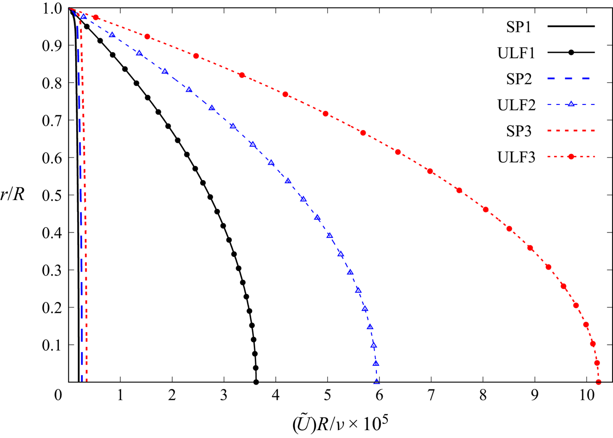
Figure 2. Mean velocity and corresponding ULF S-profiles for Princeton Superpipe flows SP1, SP2, and SP3 (see table 1).
Table 1. Princeton Superpipe experimental data and best fitting Pai polynomials for moderate  $Re$ (from García García & Fariñas Alvariño Reference García García and Fariñas Alvariño2019b).

The zero theorem for turbulent Hagen–Poiseuille flow is somewhat different, and is expressed as
 \begin{equation} Re_L = 2 \tilde{u}_L = u_L(0) =\frac{\varPi+\varGamma}{4}={-} \frac{ \sigma_w}{2} = \frac{u_{\tau}^2}{2} = \frac{64}{f_L}= \frac{16}{C_{f_L}}, \end{equation}
where  $Re_L$, $u_L(0)$, $\tilde {u}_L$ and $f_L=8 |\sigma _w|/\tilde {u}_L^2=4C_{f_L}$ refer to the ULF, whereas the MPG $\varPi$, gravity $\varGamma$, WSS $\sigma _w$ and friction velocity $u_{\tau }$ are those of the actual turbulent flow. This blend of mean-flow quantities, which can be measured directly on the flow, and those belonging to the ULF, will reveal itself as a most powerful tool. In fact, $\varPi +\varGamma$ is the quantity that can be measured most easily of all above and plays a prominent role within the TULF, as we shall see in the coming pages. Note how the zero theorem, (3.6), imposes another strong analytical constraint: given any smooth-pipe S-flow, complete laminarisation can only take place if $Re \rightarrow Re_L=(\varPi +\varGamma )/4$, or vice versa, $Re_L=(\varPi +\varGamma )/4 \rightarrow Re$, if $Re$ is kept constant. This last situation implies necessarily to decrease $\varPi +\varGamma$, which constitutes, at least, one of the driving mechanisms for complete laminarisation at constant $Re$. In any successful laminarisation instance, the PTC would be non-existent and the whole flow field would be determined by the ULF alone.
The consequences of the zero theorem are also observed in other experiments with horizontal pipes (Mullin Reference Mullin2011): if the pressure gradient of a laminar flow is slowly and gradually increased, its  $Re$ increases proportionally until transition to turbulence occurs, which is accompanied by a noticeable reduction in $Re$. Also, once the flow becomes turbulent, a proportionally ever-higher MPG must be applied to obtain each unit increase of $Re$. This additional MPG increases directly and proportionally the ULF (as in any ordinary laminar flow), and also serves to power the PTC (see figure 2); in turn, this implies that $Re_L$ grows proportionally more than $Re$ with each unit increase of MPG. The decrease of $Re$ during transition to turbulence is also predicted in Marusic et al. (Reference Marusic, Joseph and Mahesh2007, p. 471), although it is not necessarily accompanied by an adverse MPG, as suggested by those authors. Instead, the loss of bulk velocity may be due to the increased dissipation caused by the newly arisen RSSRG, source of the PTC. Conversely, as shown by (3.3a,b), any action that reduces the PTC, without modifying the MPG, will increase significantly the bulk velocity of the flow, as also suggested in Marusic et al. (Reference Marusic, Joseph and Mahesh2007, § 5).
A consequence of (3.3a,b) and boundary condition  $\sigma (1)=0$ is $\mathrm {d} u(1)/\mathrm {d} \alpha =-( \varPi +\varGamma )/2$. Equation (2.6a–c) defines $\mathrm {d} u(1)/\mathrm {d} \alpha$ as the WSS $\sigma _w$, and (2.8) confirms the well known fact that the WSS of a turbulent S-flow is coincident with that of a laminar S-flow driven by the same MPG. Thus, it follows that, in the neighbourhood of the wall, the turbulent S-flow has properties of laminar S-flow (viscous sublayer). One can check by zooming into figure 2 how each pair SPi-ULFi is coincident about the wall, including the curve's slope at $\alpha =1$. In a previous paper (García García & Fariñas Alvariño Reference García García and Fariñas Alvariño2019c), we showed that the near-wall viscous sublayer observed in turbulent Hagen–Poiseuille flow is a domain where the S-ULF prevails and the S-PTC is virtually zero. The field $u_T(\alpha )$ is negligible about the wall in any S-flow and wall-related quantities, such as $\sigma _w$ or $u_{\tau }$, are exclusively defined by the S-ULF. In other words, the viscous sublayer is the manifestation of the S-ULF in the actual physical flow, and is the region where the mathematical concept becomes real. The S-ULF is the agent directly causing wall-related stresses and constitutes a very useful notion for the study of pipe flows, and for the present research, as will be shown in § 6.
We shall now offer a very intuitive (and rigorous) demonstration of how the familiar viscous sublayer stems from the S-ULF. We begin with the laminar Hagen–Poiseuille equation that represents the S-ULF,
 \begin{equation} u_L(\alpha) = \frac{\varPi+\varGamma}{4} (1-\alpha^2). \end{equation}
The zero theorem (3.6) states that  $u_{\tau }^2 / 2 = (\varPi +\varGamma )/4$, therefore
 \begin{equation} u_L(\alpha) = \frac{u_{\tau}^2 }{2} (1-\alpha^2) \end{equation}
or
 \begin{equation} \frac{u_L(\alpha)}{ u_{\tau}} = u^+ (\alpha)= \frac{u_{\tau} }{2} (1-\alpha^2), \end{equation}
with  $u^+$ the ULF expressed in wall units. Now we write $\alpha = 1- y/R=1-\hat y$, where $y$ is the distance measured from the wall, not from the centreline as $\alpha = r/R$. Thus,
 \begin{equation} 1-\alpha^2 = 1- (1-\hat{y})^2 = 2 \hat{y} - \hat{y}^2. \end{equation}
Insert this result into (3.9), and we have
 \begin{equation} u^+ (\alpha ) = u^+ (\hat y )= \frac{u_{\tau} }{2} (2 \hat{y} - \hat{y}^2)= u_{\tau} \hat y - \frac{u_{\tau}}{2}\hat y^2 = y^+{+} O(\hat y^2). \end{equation}
Near the wall, the term  $O(\hat y^2)$ becomes negligible and we find the very expression defining the viscous sublayer, $u^+ = y^+$, which has emanated directly from the Hagen–Poiseuille equation of the S-ULF. This simple exercise furnishes two important pieces of information: (i) the viscous sublayer is the physical manifestation of the S-ULF near the wall; and (ii) the viscous sublayer is a Hagen–Poiseuille flow.
The TULF puts forward a new interpretation of the Moody chart, i.e. the relationship between the flow rate ( $Re$) and $\varPi +\varGamma$ (or the friction factor $f$) for a smooth-pipe S-flow. To understand it, we show first the general expression for the bulk velocity of turbulent Hagen–Poiseuille flow, obtained from (2.6a–c) and (3.3a,b),
 \begin{equation} \tilde{u}=\tilde{u}_L+\tilde{u}_T=\frac{\varPi+\varGamma}{8}-2\int _0^1 \mathrm{d} \alpha \ \alpha \int _{\alpha}^{1} \, \mathrm{d} \alpha' \ \sigma(\alpha'). \end{equation}
The double integral of the RSS (the bulk S-PTC) is what explains the different behaviour of the Moody chart in the turbulent region. Using (3.12) and the definition of Darcy friction factor  $f$, (2.7a,b), we get the following relationship between $f$ and the bulk S-PTC for smooth pipes:
 \begin{equation} \int _0^1 \mathrm{d} \alpha \ \alpha \int _{\alpha}^{1} \, \mathrm{d} \alpha' \sigma(\alpha') = \frac{Re}{4}\left( \frac{f \, Re}{64} -1 \right). \end{equation}
If the S-flow were laminar,  $f=64/Re$ and the expression between brackets would be zero. Equation (3.13) shows that for any smooth-pipe S-flow of given $Re$ there is a one-to-one mapping between $f$ and the double integral of the RSS (or bulk S-PTC). And also, that the wall-roughness changes the distribution of RSS within a pipe flow, for given $Re$.
$Re$.
To end this section, the TULF brings forth a very intuitive field to assess, just at a glance, how turbulent a mean flow is in a given region. This scalar field is called the turbulence index  $\mathfrak {I}(\alpha )$, and is defined as the ratio of the mean velocity to the ULF (see García García & Fariñas Alvariño Reference García García and Fariñas Alvariño2019c, Reference García García and Fariñas Alvariño2020, Reference García García and Fariñas Alvariño2021),
 \begin{equation}
\mathfrak{I}(\alpha)= \frac{u(\alpha)}{u_L(\alpha)}=1+
\frac{u_T(\alpha)}{u_L(\alpha)},
\end{equation}
\begin{equation}
\mathfrak{I}(\alpha)= \frac{u(\alpha)}{u_L(\alpha)}=1+
\frac{u_T(\alpha)}{u_L(\alpha)},
\end{equation}
with  $0<\mathfrak {I}\leq 1$ in a S-flow, and $\mathfrak {I}= 1$ in regions where the flow is mean laminar; that is, in regions where $u_T=0$. We shall see later that $\mathfrak {I}(\alpha )$ is very useful in determining where a turbulent flow is laminarised, and the degree of laminarisation it presents. The turbulence index thereby defined is itself a mean scalar field that measures, at each point, how much the mean velocity departs from the ULF. The turbulence is seen as an agent that detaches the flow from its best possible configuration, which is the ULF. A turbulent Hagen–Poiseuille flow verifies $\lim _{\alpha \rightarrow 1} \mathfrak {I}(\alpha )= 1$; otherwise put, the viscous sublayer is a retrodiction of the TULF, see García García & Fariñas Alvariño (Reference García García and Fariñas Alvariño2019c) and (3.11).
It is also possible to define the bulk turbulence index
 \begin{equation} \tilde{\mathfrak{I}} = 2 \int _0^1 \alpha \mathfrak{I}(\alpha) \, \mathrm{d} \alpha, \end{equation}
with which the complete S-flow is characterised by a single real number  $0< \tilde {\mathfrak {I}} \leq 1$. Note $\tilde {\mathfrak {I}} =1$ in laminar S-flow, i.e. in Hagen–Poiseuille flow.
4. Turbulent Hagen–Poiseuille–Couette pipe flow
Although the experiment with a sliding pipe segment will not be explained in this paper, for the sake of completeness we shall also consider briefly the mixed fully developed turbulent steady-state Hagen–Poiseuille–Couette mean pipe flow, or simply turbulent Hagen–Poiseuille–Couette flow, in which the flow is driven by a constant  $\varPi +\varGamma$, a constant RSSRG $\varSigma (\alpha )=-(1/\alpha ) \, \mathrm {d}(\alpha \sigma )/\mathrm {d} \alpha$ and a pipe moving in the streamwise direction with constant velocity $V_w$ (see figure 1). The governing equation for such a mean flow is also (3.2), together with the boundary conditions,
 \begin{equation} u(1)=V_w , \quad \frac{\mathrm{d} u(0)}{\mathrm{d} \alpha}=0 , \quad \sigma(0)=\sigma(1)=0, \end{equation}
where  $V_w$ is the constant velocity of the pipe's wall in the natural normalisation. The solution for the turbulent Hagen–Poiseuille–Couette flow is
 \begin{equation} u(\alpha)=V_w + \frac{\varPi+\varGamma}{4} (1-\alpha^2)- \int _{\alpha}^1 \sigma(\alpha') \, \mathrm{d} \alpha', \quad \sigma(\alpha)= \frac{\mathrm{d} u}{\mathrm{d} \alpha} + \frac{\varPi+\varGamma}{2} \alpha, \end{equation}
thereby the wall velocity  $V_w$ is added to $(\varPi +\varGamma )(1-\alpha ^2)/4$ to yield the S-ULF,
 \begin{equation} u_L(\alpha)=V_w + \frac{\varPi+\varGamma}{4} (1-\alpha^2), \end{equation}
which is coincident with the laminar Hagen–Poiseuille–Couette velocity field. Note this RSS  $\sigma (\alpha )$ is formally indistinguishable from that of the turbulent Hagen–Poiseuille flow, (3.3a,b); this follows from the fact that the mean field $u_w(\alpha )\equiv u(\alpha )-V_w$ is, from a mathematical standpoint, a turbulent Hagen–Poiseuille flow with the same sources $\varPi +\varGamma$ and $\varSigma (\alpha )$. We shall use this result later in § 7.1.
The zero theorem for turbulent Hagen–Poiseuille–Couette flow is not too different from the turbulent Hagen–Poiseuille flow, and with the same nomenclature takes the form
 \begin{align} Re_L
&= 2\tilde{u}_L=2 V_w+\frac{\varPi+\varGamma}{4}=V_w+u_L(0)=
2 V_w - \frac{ \sigma_w}{2}\nonumber\\
& = 2 V_w + \frac{u_{\tau}^2}{2}
= \frac{64 (\varPi+\varGamma)}{f_L (8
V_w+\varPi+\varGamma)},
\end{align}
\begin{align} Re_L
&= 2\tilde{u}_L=2 V_w+\frac{\varPi+\varGamma}{4}=V_w+u_L(0)=
2 V_w - \frac{ \sigma_w}{2}\nonumber\\
& = 2 V_w + \frac{u_{\tau}^2}{2}
= \frac{64 (\varPi+\varGamma)}{f_L (8
V_w+\varPi+\varGamma)},
\end{align}
with  $f_L=8|\sigma _w|/\tilde {u}_L^2=4C_{f_L}$. Again, note how the knowledge of $\varPi +\varGamma$ and $V_w$ permits to determine the relevant quantities of the S-flow, and also that (4.4) provides a necessary condition for the flow to become laminar: any attempt to approximate $Re$ to $Re_L=2 V_w+(\varPi +\varGamma )/4$, or vice versa, would laminarise the flow and increase the turbulence index field.
We also end this section with the general expression for the bulk velocity of turbulent Hagen–Poiseuille–Couette flow, obtained from (2.6a–c) and (4.2a,b),
 \begin{equation} \tilde{u}=\tilde{u}_L+\tilde{u}_T=V_w+\frac{\varPi+\varGamma}{8}- 2\int _0^1 \mathrm{d} \alpha \ \alpha \int _{\alpha}^{1} \, \mathrm{d} \alpha' \sigma(\alpha'). \end{equation}
5. General incompressible fully developed mean pipe flow
We have just covered the most important instances of pipe S-flow. Now we shall consider the case of general incompressible fully developed mean flow, regardless of its being steady, unsteady, laminar or turbulent. As mentioned in § 3, this exercise is entirely developed in the mean space  $\mathfrak {M}$.
Let the incompressible fully developed pipe flow be as shown in figure 1, which we assume circularly symmetric on average, i.e.  $\partial \varPsi / \partial \theta =0$ for any mean-flow quantity $\varPsi \in \mathfrak {M}$. Mean-flow quantities are supposed the result of an ensemble-average over denumerable infinite realisations of the same flow, see García García (Reference García García2017, § 3.2.1). The flow is actuated upon by a MPG $\varPi (\tau )$ and a RSSRG $\varSigma (\tau,\alpha )$, the pipe wall is moving streamwise with dimensionless velocity $V_w(\tau )$, and it is undergoing the force of gravity. The angle $\varTheta =\varTheta (\tau )$ is assumed variable, always provided its variation causes negligible radial and azimuthal mean-velocity components, i.e. the mean flow always remains one-directional along the pipe's axis. A pipe-wall velocity $V_w(\tau )$ could be interpreted as a sliding pipe, as in Kuehnen et al. (Reference Kuehnen, Song, Scarselli, Budanur, Riedl, Willis, Avila and Hof2018b), or, for example, as the flow created in the longitudinal pipes of a decelerating train, or any other moving vessel. Leaving aside electromagnetic forces and fancy effects, like spinning or shaking pipes, the flow illustrated in figure 1 would rank as rather comprehensive. The action of gravity is expressed in the natural normalisation as the following time-dependent dimensionless quantity:
 \begin{equation} \varGamma(\tau)=\frac{g R^3 \cos \varTheta(\tau)}{\nu^2}. \end{equation}
We neglect the difference in gravity across the pipe diameter, for it would lead to circular-symmetry breaking. At  $\tau =0$, which is taken as the initial instant without loss of generality, the mean-velocity field within the pipe is
 \begin{equation} u_0(\alpha)=u_{0_L}(\alpha)+u_{0_T}(\alpha) , \quad u_0\in \mathfrak{M}, \end{equation}
which is decomposed into an ULF and a PTC. Here  $u_0(\alpha )$ might be a S-flow or the frozen profile at $\tau =0$ of any U-flow, thus corresponding to real mean flows, or it could be any arbitrary smooth function fulfilling the boundary conditions. Let also $V_{w_0}=V_w(0)\in \mathbb {R}$ be the initial velocity at $\tau =0$ of the pipe's wall.
The governing equation for the dynamical system thus described is the RANSE, which in the natural normalisation adopts the form
 $$\begin{gather} \frac{\partial u}{\partial \tau}-\left( \frac{\partial^2 u}{\partial \alpha^2}+\frac{1}{\alpha}\frac{\partial u}{\partial \alpha}\right) =\varPi(\tau) +\varGamma(\tau)-\frac{1}{\alpha}\frac{\partial (\alpha \sigma)}{\partial \alpha}=\varPi(\tau)+\varGamma(\tau)+ \varSigma(\tau,\alpha), \end{gather}$$
 $$\begin{gather}\alpha \in (0,1), \quad \tau \in \mathbb{R}^+, \quad u,\varPi,\varGamma, \sigma,\varSigma \in \mathfrak{M}, \end{gather}$$
subject to the boundary conditions in  $\alpha =0$ and $\alpha =1$,
 \begin{equation} u(\tau,1)=V_w(\tau) , \quad \frac{\partial u(\tau,0)}{\partial \alpha}=0 , \quad \sigma(\tau,0)=\sigma(\tau,1)=0 \end{equation}
and to the initial condition for  $\tau =0$,
 \begin{equation} u(0,\alpha)=u_0(\alpha)=u_{0_L}(\alpha)+u_{0_T}(\alpha), \end{equation}
plus the dimensionless Reynolds-averaged continuity equation,
 \begin{equation} \frac{\partial u(\tau,\alpha)}{\partial \beta}=0, \end{equation}
which is trivial in this case. The boundary condition at  $\alpha =0$, $\partial u(\tau,0)/\partial \alpha =0$, is necessary to maintain the circular symmetry of the mean flow (independence of azimuth coordinate $\theta$), since only mean-velocity fields with continuous derivatives are acceptable as solutions. Equation (5.3) is a non-homogeneous parabolic partial differential equation for the function $u(\tau,\alpha )$, and the function $\varPi (\tau )+\varGamma (\tau )+\varSigma (\tau,\alpha )$ is called the non-homogeneous term in mathematics texts, the input in signal analysis theory, or the source in electrodynamics parlance, which is the usage we shall adopt herein. The mean field $\varSigma (\tau,\alpha )$ is called the RSSRG. Note the different role of the sources involved in (5.3): $\varPi (\tau )$ and $\varGamma (\tau )$ contribute to create motion in the fluid and may be loosely called active forces or agents, whereas $\varSigma (\tau,\alpha )$ is meant to dissipate energy from the flow and thus deserves the name of reactive force or agent. $V_w(\tau )$ qualifies also as an active agent, because it transmits momentum to the flow, but it is not itself a force, although a force is needed to set in motion the pipe's wall. Likewise, $\sigma (\tau,\alpha )$ would be a reactive agent, albeit not a force by itself.
The TULF considers the mean flow as a dynamical system, whose evolution is described and explained through its governing equation (5.3), in which the sources (inputs) cause the changes in the mean-velocity field (output). Here  $V_w(\tau )$ is not a mathematical source of motion, but a boundary condition that contributes to imparting momentum. A force (and thus a source of motion) makes the wall move, which is indirectly transmitted to the fluid to cause flow.
Equation (5.3) is solved considering first the associated homogeneous equation, i.e. the same expression with  $\varPi +\varGamma +\varSigma \equiv 0$ and zero boundary conditions, $V_w\equiv 0$. After separation of variables, the homogeneous equation in $\alpha$ corresponds to the eigenvalue problem for the Laplace operator in the open unit disc with rotational ( $\partial /\partial \theta = 0$) and axial ( $\partial / \partial z =0$) symmetry (see García García (Reference García García2017, § 3.4.2) and García García & Fariñas Alvariño (Reference García García and Fariñas Alvariño2019b)),
 \begin{equation} \frac{1}{\alpha} \frac{\mathrm{d} \phi}{\mathrm{d} \alpha}+\frac{\mathrm{d}^2 \phi}{\mathrm{d} \alpha^2}={-}\lambda^2 \phi , \quad \phi(1)=0, \alpha \in (0,1), \ \lambda \in \mathbb{R}, \end{equation}
which constitutes a classical Sturm–Liouville problem whose solution is the set of normalised eigenfunctions,
 \begin{equation} \phi_n(\alpha)=\frac{\sqrt{2}\ J_0(\lambda_n \alpha)}{J_1(\lambda_n)}, \end{equation}
with  $\lambda _n$ the $n$th root (or zero) of $J_0(\alpha )$, the Bessel function of the first kind of order zero. Being a Sturm–Liouville eigenvalue problem, it is guaranteed that the set $\{\phi _n(\alpha )\}$ constitutes an orthonormal basis of the weighted Hilbert space of square-integrable functions in the interval $(0, 1)$, see García García (Reference García García2017, § 3.4.2) and García García & Fariñas Alvariño (Reference García García and Fariñas Alvariño2019b). Among other things, this last statement means that any mean field $\varPsi (\tau,\alpha ) \in \mathfrak {M}\subset L^2_{\alpha }(0,1)$ can be uniquely expressed in the basis $\{\phi _n(\alpha )\}$ as
 \begin{equation} \varPsi(\tau,\alpha)=\sum _{n=1}^{\infty} \langle \varPsi, \phi_n \rangle \phi_n=\sum _{n=1}^{\infty} \varPsi_n(\tau) \phi_n(\alpha), \end{equation}
whereby  $\langle \varPsi,\phi _n \rangle$ is the inner product naturally defined in the weighted Hilbert space $L^2_{\alpha }(0,1)$, namely
 \begin{equation} \varPsi_n(\tau) =\langle \varPsi,\phi_n \rangle \equiv \int _0^1 \alpha \varPsi(\tau,\alpha) \phi_n(\alpha) \, \mathrm{d} \alpha. \end{equation}
Every function appearing in (5.3)–(5.6) has its corresponding expansion in a Fourier–Bessel series as in (5.10). Thereby, making good use of the mathematical apparatus of partial differential equations and functional analysis in Hilbert spaces, the general analytic solution for incompressible fully developed mean pipe flow is obtained, which takes the form (García García (Reference García García2017, § 3.4.2); García García & Fariñas Alvariño (Reference García García and Fariñas Alvariño2019b)),
 \begin{align} u(\tau,\alpha)&=\sum
_{n=1}^{\infty} u_n(\tau) \phi_n(\alpha)= \sum
_{n=1}^{\infty} ( u_{I_{L_n}}+u_{P_{n}}+u_{G_{n}}+u_{W_{n}}
+u_{I_{T_n}}+u_{R_{n}} ) \phi_n(\alpha) \nonumber\\ &=\sum
_{n=1}^{\infty} \left \{ \left( u_{L_n}^{(0)}-
\frac{\sqrt{2}V_{w_0}}{\lambda_n} \right)\,
\mathrm{e}^{-\lambda_n^2 \tau} +
\frac{\sqrt{2}}{\lambda_n}\int _0^{\tau} [\varPi(\tau') +
\varGamma(\tau')] \mathrm{e}^{-\lambda_n^2 (\tau-\tau')} \,
\mathrm{d}\tau' \right. \nonumber\\ &\quad
+\frac{\sqrt{2}}{\lambda_n} \left( V_w(\tau) - \int
_0^{\tau} \dot{V}_w(\tau')\, \mathrm{e}^{-\lambda_n^2
(\tau-\tau')} \, \mathrm{d}\tau' \right) \nonumber\\ &
\left. \quad +u_{T_n}^{(0)} \mathrm{e}^{-\lambda_n^2 \tau}
+ \int _0^{\tau} \varSigma_n(\tau')\,
\mathrm{e}^{-\lambda_n^2(\tau- \tau')} \, \mathrm{d}\tau'
\right\}\frac{\sqrt{2} J_0(\lambda_n
\alpha)}{J_1(\lambda_n)} = u_L(\tau,\alpha) +
u_T(\tau,\alpha), \end{align}
\begin{align} u(\tau,\alpha)&=\sum
_{n=1}^{\infty} u_n(\tau) \phi_n(\alpha)= \sum
_{n=1}^{\infty} ( u_{I_{L_n}}+u_{P_{n}}+u_{G_{n}}+u_{W_{n}}
+u_{I_{T_n}}+u_{R_{n}} ) \phi_n(\alpha) \nonumber\\ &=\sum
_{n=1}^{\infty} \left \{ \left( u_{L_n}^{(0)}-
\frac{\sqrt{2}V_{w_0}}{\lambda_n} \right)\,
\mathrm{e}^{-\lambda_n^2 \tau} +
\frac{\sqrt{2}}{\lambda_n}\int _0^{\tau} [\varPi(\tau') +
\varGamma(\tau')] \mathrm{e}^{-\lambda_n^2 (\tau-\tau')} \,
\mathrm{d}\tau' \right. \nonumber\\ &\quad
+\frac{\sqrt{2}}{\lambda_n} \left( V_w(\tau) - \int
_0^{\tau} \dot{V}_w(\tau')\, \mathrm{e}^{-\lambda_n^2
(\tau-\tau')} \, \mathrm{d}\tau' \right) \nonumber\\ &
\left. \quad +u_{T_n}^{(0)} \mathrm{e}^{-\lambda_n^2 \tau}
+ \int _0^{\tau} \varSigma_n(\tau')\,
\mathrm{e}^{-\lambda_n^2(\tau- \tau')} \, \mathrm{d}\tau'
\right\}\frac{\sqrt{2} J_0(\lambda_n
\alpha)}{J_1(\lambda_n)} = u_L(\tau,\alpha) +
u_T(\tau,\alpha), \end{align}
with  $\dot {V}_w \equiv \mathrm {d} V_w/\mathrm {d} \tau$, and $u_{L_n}^{(0)}$ and $u_{T_n}^{(0)}$ the components in the Fourier–Bessel series of the ULF and PTC, respectively, of the initial mean-velocity field $u_0(\alpha )$, according to (5.10). The remaining components will be defined next.
Note the analogous role played by MPG  $\varPi (\tau )$ and gravity $\varGamma (\tau )$ in the solution (5.12); many effects obtained with a MPG in the mean flow can also be attained through gravity and a suitable inclination. The mean-velocity field $u(\tau,\alpha )$ has two main components, the ULF and the PTC. The subcomponents of the ULF $u_L(\tau,\alpha )$ arise from the active forces or agents and are the following.
(i) The term derived from initial conditions, called the ULF of IniTrans $u_I(\tau,\alpha )$,
(5.13)which typically is also dependent upon the value of active agents for\begin{equation} u_{I_L}(\tau,\alpha)=\sum _{n=1}^{\infty}u_{I_{L_n}}\phi_n (\alpha) =\sum _{n=1}^{\infty} \left( u_{L_n}^{(0)}- \frac{\sqrt{2}V_{w_0}}{\lambda_n} \right)\, \mathrm{e}^{-\lambda_n^2 \tau} \phi_n (\alpha), \end{equation}$\tau \leq 0$.
$u_I(\tau,\alpha )$,
(5.13)which typically is also dependent upon the value of active agents for\begin{equation} u_{I_L}(\tau,\alpha)=\sum _{n=1}^{\infty}u_{I_{L_n}}\phi_n (\alpha) =\sum _{n=1}^{\infty} \left( u_{L_n}^{(0)}- \frac{\sqrt{2}V_{w_0}}{\lambda_n} \right)\, \mathrm{e}^{-\lambda_n^2 \tau} \phi_n (\alpha), \end{equation}$\tau \leq 0$.(ii) The term derived from MPG
$\varPi (\tau )$, called PresGrad,
(5.14)\begin{equation} u_{P}(\tau,\alpha)=\sum _{n=1}^{\infty}u_{P_{n}}\phi_n (\alpha) =\sum _{n=1}^{\infty} \frac{\sqrt{2}}{\lambda_n} \phi_n(\alpha) \int _0^{\tau} \varPi(\tau')\, \mathrm{e}^{-\lambda_n^2 (\tau-\tau')} \, \mathrm{d}\tau'. \end{equation}(iii) The term derived from gravity
$\varGamma (\tau )$, called Gravit,
(5.15)\begin{equation} u_{G}(\tau,\alpha)=\sum _{n=1}^{\infty}u_{G_{n}}\phi_n (\alpha) =\sum _{n=1}^{\infty}\frac{\sqrt{2}}{\lambda_n} \phi_n(\alpha) \int _0^{\tau} \varGamma(\tau')\,\mathrm{e}^{-\lambda_n^2 (\tau-\tau')} \, \mathrm{d}\tau'. \end{equation}(iv) The term derived from the wall-velocity boundary condition, called Wallit,
(5.16)\begin{equation} u_{W}(\tau,\alpha)=\sum _{n=1}^{\infty}u_{W_{n}}\phi_n (\alpha) =\sum _{n=1}^{\infty} \frac{\sqrt{2}}{\lambda_n}\left( V_w(\tau) - \int _0^{\tau} \dot{V}_w(\tau')\, \mathrm{e}^{-\lambda_n^2 (\tau-\tau')} \, \mathrm{d}\tau' \right) \phi_n(\alpha). \end{equation}


On the other hand, the subcomponents of the PTC  $u_T(\tau,\alpha )$ spring from reactive forces or agents, namely (v) and (vi), next.
(v) The term derived from initial conditions, called the PTC of IniTrans
$u_I(\tau,\alpha )$,
(5.17)which normally is also dependent upon the value of reactive agents for\begin{equation} u_{I_T}(\tau,\alpha)=\sum _{n=1}^{\infty} u_{I_{T_n}}\phi_n (\alpha) =\sum _{n=1}^{\infty} u_{T_n}^{(0)} \mathrm{e}^{-\lambda_n^2 \tau} \phi_n (\alpha), \end{equation}$\tau \leq 0$.(vi) The term derived from the RSSRG
$\varSigma (\tau,\alpha )$, called RStress,
(5.18)\begin{equation} u_{R}(\tau,\alpha)=\sum _{n=1}^{\infty}u_{R_{n}}\phi_n (\alpha) = \sum _{n=1}^{\infty}\phi_n(\alpha) \int _0^{\tau} \varSigma_n(\tau')\, \mathrm{e}^{-\lambda_n^2 (\tau-\tau')} \,\mathrm{d}\tau'. \end{equation}


From (5.13) and (5.17) follows the complete expression of the component IniTrans,  $u_I(\tau,\alpha )=u_{I_L}(\tau,\alpha )+u_{I_T}(\tau,\alpha )$. To the authors’ knowledge, this is the first time such a comprehensive solution for general fully developed mean pipe flow has ever been written.
From the above relationships it follows that active agents cause exclusively the ULF, whereas reactive agents cause exclusively the PTC. As a general rule, active agents are those appearing in the Navier–Stokes equation from which the RANSE stems, whereas reactive agents belong exclusively to the RANSE; no Reynolds stresses appear in the Navier–Stokes equations.
We must repeat that (5.12) is the general solution for fully developed mean pipe flow, with governing equations (5.3)–(5.7). Any actual fully developed mean pipe flow must be written in this form and, conversely, any given expression of the form (5.12) would correspond to the unique mean flow obtained if the sources (forces)  $\varPi (\tau )$, $\varGamma (\tau )$ and $\varSigma (\tau,\alpha )$, and the boundary and initial conditions $V_w(\tau )$ and $u_0(\alpha )$, were actually actuating upon the flow. The S-flows discussed in previous sections are all expressible in the form (5.12). The problem is now reduced to finding the appropriate functions $\varPi (\tau )$, $\varGamma (\tau )$, $\varSigma (\tau,\alpha )$, $V_w(\tau )$ and $u_0(\alpha )$ for any reported flow, to the maximum degree of accuracy. This can be done by measurements in real flows or from computational fluid dynamics simulations. When data is scarce, or simply not available, one can always presume, ad hoc, some functions (inputs) and check whether the resulting mean-velocity field (the output) would be accurate enough to reproduce the actual flow. We have already performed such a type of exercise in our previous papers (García García & Fariñas Alvariño Reference García García and Fariñas Alvariño2019a,Reference García García and Fariñas Alvariñob,Reference García García and Fariñas Alvariñoc, Reference García García and Fariñas Alvariño2020, Reference García García and Fariñas Alvariño2021), which we call ‘theoretical experiments’, and the results were satisfactory and provided true explanations for the observed facts, also allowing us to issue predictions that still await confirmation. Regardless of the procedure, the set of particular functions $\varPi (\tau )$, $\varGamma (\tau )$, $\varSigma (\tau,\alpha )$, $V_w(\tau )$ and $u_0(\alpha )$ chosen for any given application is called the ‘model’. We shall select particular functions in § 7 to explain the laminarisation process observed in the experiments of Kuehnen et al. (Reference Kuehnen, Song, Scarselli, Budanur, Riedl, Willis, Avila and Hof2018b), which would justify the title given to the present research work. We are aware that the solution furnished by (5.12) is rather complicated, but so is the problem that it is meant to solve. Surely, the reader would not expect any easy solution for a century-old unsolved problem.
We would like to highlight the parallel roles of mean pressure and RSS in the mean flow. The RSS plays for the PTC a similar role that the mean pressure plays for the ULF: what it really counts is the gradient, not the quantity itself. In the case of the ULF it is the streamwise gradient (of mean pressure) and in the case of the PTC is the radial gradient (of RSS). A flow can have very high levels of mean pressure or of RSS, but if their gradients are small, then so would be the corresponding mean fields, ULF and PTC.
The turbulence index field for this general mean flow is also defined as
 \begin{equation} \mathfrak{I}(\tau,\alpha)= \frac{u(\tau,\alpha)}{u_L(\tau,\alpha)}=1+ \frac{u_T(\tau,\alpha)}{u_L(\tau,\alpha)}, \end{equation}
with  $u$,
$u$,  $u_L$ and $u_T$ given by the expressions above. Unlike its steady-state counterpart, (3.14), the turbulence index of (5.19) can be greater than $1$. In those space–time domains with $\mathfrak {I}(\tau,\alpha )>1$ the U-flow is said to be hyperlaminar, for the mean velocity would be greater than that corresponding to purely laminar U-flow (to the U-ULF). Otherwise put, the turbulence would create an additional positive mean velocity that adds up to the laminar component; instead of dissipating energy, the turbulence forces would cooperate to locally erect some new mean velocity. Within a spatial region, and during a time interval, the reactive forces would become active and would contribute to create fresh motion. Outstanding experimental examples of hyperlaminarity are observed in Annus et al. (Reference Annus, Koppel, Sarv and Ainola2013, figure 3) and Mathur et al. (Reference Mathur, Gorji, He, Seddighi, Vardy, O'Donoghue and Pokrajac2018, figure 5). We consider hyperlaminarity one of the most interesting and intriguing phenomena in the current panorama of fluid mechanics, and we shall devote further research articles to its study.
The bulk velocity  $\tilde {u}(\tau )$ corresponding to the mean velocity $u(\tau,\alpha )$ of (5.12) is given by
 \begin{align} \tilde{u}(\tau)&=2 \sqrt{2}\sum _{n=1}^{\infty} \frac{u_n(\tau)}{\lambda_n}=2 \sqrt{2}\sum _{n=1}^{\infty} \frac{1}{\lambda_n} \left( u_{I_{L_n}}+u_{P_{n}}+u_{G_{n}}+u_{W_{n}}+u_{I_{T_n}}+u_{R_{n}} \right ) \nonumber\\ &=4 \sum _{n=1}^{\infty} \left \{ \left( \frac{u_{L_n}^{(0)}}{\sqrt{2}}-\frac{V_{w_0}}{\lambda_n} \right) \frac{\mathrm{e}^{-\lambda_n^2 \tau}}{\lambda_n} + \frac{1}{\lambda_n^2} \int _0^{\tau} [\varPi(\tau') + \varGamma(\tau')] \, \mathrm{e}^{-\lambda_n^2 (\tau-\tau')} \, \mathrm{d}\tau' \right. \nonumber\\ &\quad +\frac{1}{\lambda_n^2} \left( V_w(\tau) - \int _0^{\tau} \dot{V}_w(\tau')\, \mathrm{e}^{-\lambda_n^2 (\tau-\tau')} \, \mathrm{d}\tau' \right) \nonumber\\ & \quad \left. +\frac{u_{T_n}^{(0)}}{\sqrt{2}} \frac{\mathrm{e}^{-\lambda_n^2 \tau}}{\lambda_n} + \frac{1}{\sqrt{2} \lambda_n}\int _0^{\tau} \varSigma_n(\tau')\, \mathrm{e}^{-\lambda_n^2(\tau- \tau')} \, \mathrm{d}\tau' \right\} = \tilde{u}_L(\tau) + \tilde{u}_T(\tau), \end{align}
and the bulk turbulence index corresponding to (5.19) is defined by
 \begin{equation} \tilde{\mathfrak{I}}(\tau) = 2 \int _0^1 \alpha \, \mathfrak{I}(\tau,\alpha) \, \mathrm{d} \alpha. \end{equation}
6. Explanation of experiments destabilising turbulence in pipe flow
What we have exposed so far are indisputable mathematical results that explain the ensemble-average behaviour of fully developed pipe flow. With these tools, we now approach the task of explaining the relevant experiments on destabilising turbulence in pipe flow of Kuehnen et al. (Reference Kuehnen, Song, Scarselli, Budanur, Riedl, Willis, Avila and Hof2018b). Since no gravity effects or pipe-wall velocity are applicable to such experiments, we shall consider (5.12) and (5.20) with  $\varGamma =V_w=V_{w_0}=\dot {V}_w=0$. In this case, PresGrad $u_P$ is the main component of the ULF, $u_L=u_{I_L}+u_P$, and frequently we shall say the MPG $\varPi$ is the source of the ULF, albeit rigorously $\varPi (\tau )$ for $\tau >0$ determines PresGrad, while $u_{I_L}$ normally depends on the MPG for $\tau \leq 0$. Likewise, we shall say the RSSRG $\varSigma$ is the source of the PTC, albeit rigorously $\varSigma (\tau,\alpha )$ for $\tau >0$ determines RStress, while $u_{I_T}$ most often depends upon the RSSRG for $\tau \leq 0$.
Let us summarise the set of facts needed for such explanations (in all that follows, the expression ‘under its own dynamics’ should be understood as ‘the field follows the evolution of its source (force) according to the governing equation’).
(i) A constant
$Re$, i.e. a constant bulk velocity $\tilde {u}$, is enforced on each experiment, that is, ULF and PTC cannot change independently (see figure 4).(ii) The zero theorem is (quasi)applicable in (quasi)S-flows. The zero theorem is only an approximation if the flow is not fully developed or slightly unsteady.
(iii) With
$\tilde {u}$ constant, the equation $\varPi =-2\sigma _w$ is a mathematical necessity, regardless of the flow being unsteady or stationary.(iv) Changes of pressure are transmitted (almost) instantaneously all over the flow, for it is considered incompressible; however, changes in MPG and WSS would take some time to propagate within the flow, for inertia plays a role in U-flows.
(v) Under its own dynamics, the ULF tends to follow the behaviour of the MPG, for
$\varPi (\tau )$ is the source of $u_L(\tau,\alpha )$ (García García & Fariñas Alvariño Reference García García and Fariñas Alvariño2019b,Reference García García and Fariñas Alvariñoc, Reference García García and Fariñas Alvariño2020, Reference García García and Fariñas Alvariño2021). The ${u}_L(\tau,\alpha )$ reacts rather quickly to changes in $\varPi (\tau )$, although it does not trail the MPG evolution instantaneously.(vi) Under its own dynamics, the PTC tends to follow the behaviour of the RSSRG, for
$\varSigma (\tau,\alpha )$ is the source of $u_T(\tau,\alpha )$ (García García & Fariñas Alvariño Reference García García and Fariñas Alvariño2019b,Reference García García and Fariñas Alvariñoc, Reference García García and Fariñas Alvariño2020, Reference García García and Fariñas Alvariño2021). In general, ${u}_T(\tau,\alpha )$ reacts more slowly than ${u}_L(\tau,\alpha )$.(vii) Close to the wall, in the viscous sublayer, the S-PTC is negligible and can be safely ignored (García García & Fariñas Alvariño (Reference García García and Fariñas Alvariño2019c) and (3.11)). In slightly unsteady flow this statement is approximately valid, whereas it is not in case of strongly accelerated/decelerated flow (García García & Fariñas Alvariño Reference García García and Fariñas Alvariño2020).
(viii) Upon changes in
$\varPi (\tau )$, the U-ULF $u_L(\tau,\alpha )$ would try to follow the evolution of $\varPi (\tau )$ according to its own time constants (see (7.23)), and $u_L(\tau,\alpha )$ will no longer be a laminar Hagen–Poiseuille flow. Thereby, $u_L(\tau,\alpha )$ and $\varPi (\tau )$ become uncoupled, meaning that even if $\varPi (\tau )$ becomes constant for $\tau \geq \tau _1$, $u_L(\tau,\alpha )$ would still be changing for $\tau \geq \tau _1$. However, $u_L(\tau,\alpha )$ has a bulk velocity $\tilde {u}_L(\tau )$, i.e. a Reynolds number $Re_L(\tau )$, which can be matched to a virtual laminar Hagen–Poiseuille flow $u^S(\alpha ;\tau )=\varPi _L(\tau )(1-\alpha ^2)/4$, such that $Re_L(\tau )=\varPi _L(\tau )/4$, or $\tilde {u}_L(\tau ) =\tilde {u}^S(\tau )$, for any time $\tau$. This continuous sequence of virtual Hagen–Poiseuille flows $u^S(\alpha ;\tau )$, each corresponding to $u_L(\tau,\alpha )$ for each time $\tau$, permits us to associate naturally an instantaneous MPG to the U-ULF (and mean velocity), so that we can compare $\varPi _L(\tau )$ with $\varPi (\tau )$ (the source), and evaluate how far the U-flow is from reaching the agent causing its motion, $\varPi (\tau )$ (recall in U-flow it is $\varPi (\tau ) \neq \varPi _L(\tau )$ but $\tilde {u}_L(\tau ) =\tilde {u}^S(\tau )$). Whenever $\varPi _L(\tau )=\varPi (\tau )$ the ULF and MPG will become coupled, which implies $\varPi ={\rm const}.$ and $Re_L=Re$, which is also constant. We shall call the continuous sequence of virtual laminar Hagen–Poiseuille flows $u^S(\alpha ;\tau )$ the steady-bulk flow (SB-flow), associated with the U-flow $u_L(\tau,\alpha )$.(ix) In any S-flow the MPG, the ULF, the RSSRG, the PTC and the mean velocity are always coupled.
(x) It must be understood that the TULF cannot issue accurate predictions over the flow's behaviour in regions where the flow is not fully developed.


Before beginning the actual explanation, let us discuss two potential naïve explanations that someone might suggest (after a first impression with scarce reflection) as the cause for the observed behaviour. (a) The external disturbance affects the ULF very little but destabilises the PTC, which is no longer able to maintain itself, and farther downstream we arrive at the outcome  $u_T(\alpha ) \approx 0$. Thus, the only surviving component would be the ULF, which is laminar, and this is the result we witness in the experiments, a lone laminar ULF. However, this scenario is not possible, because the surviving ULF would have a much greater Reynolds number than the original flow, $Re_L \gg Re$ (see figure 2), and what we witness is a flow that does not change its Reynolds number. Therefore, a true explanation must also account for a radical reduction in ULF. (b) The external disturbance modifies the RSS $\sigma (\alpha )$ in such a way that the resultant flow would be parabolic. For example, if $\sigma (\alpha )=K \alpha$ for constant $K$, then (3.5) implies $u_T(\alpha )=-K (1-\alpha^2)/2$, and the mean velocity would be $u(\alpha )=u_L+u_T=(\varPi - 2K) (1-\alpha^2)/4$, which resembles a parabolic Hagen–Poiseuille flow with effective MPG $\varPi -2K$, supposedly in agreement with the experiments. Neither would this outcome be possible, for two reasons: (1) the resulting flow, however parabolic, would still be turbulent, for the PTC would not be zero ( $u_T\neq 0$); and (2) a RSS with the functional form $\sigma (\alpha )=K\alpha$ would not fulfil the no-slip boundary condition at the wall, $\sigma (1)=0$. The immediate conclusion is that a PTC cannot be parabolic. Therefore, none of those naïve explanations would qualify as a true explanation. The examples above are offered to illustrate that tampering with numbers, without solid physics foundations, is a practice that frequently leads to erroneous results.
6.1. Statement of the problem
Firstly, it must be observed that this problem has two natural parabolic variables, in the sense of partial differential equations theory: time  $\tau$ and axial streamwise coordinate $\beta =z/R$. As the Reynolds number is constant in those experiments, we can establish a linear mapping between them as follows:
 \begin{equation} \beta=\tau \, Re / 2, \end{equation}
whereby the dynamic behaviour could either be described in terms of  $\tau$ or $\beta$. Due to the character of the TULF, we shall be using $\tau$ in our reasoning. Moreover, we shall consider horizontal pipes and henceforth it will be assumed $\varGamma =0$ everywhere.
The statement of the physico-mathematical problem is as follows (see figure 3). We begin with a horizontal turbulent S-flow characterised by  $\varPi _0$ and $Re=2\tilde {u}$, satisfying the zero theorem (3.6) with $Re_{L_0}>Re$ (and possibly $Re_{L_0} \gg Re$), which we wish to convert into a laminar Hagen–Poiseuille flow defined by $\varPi _f(1-\alpha ^2)/4=Re (1-\alpha ^2)$, with $\varPi _f<\varPi _0$ (and possibly $\varPi _f \ll \varPi _0$) and the same $Re=Re_{L_f}=2\tilde {u}$, fulfilling the zero theorem (2.8) with $\varPi _f=4Re$; that is, we must decrease considerably the MPG while maintaining constant the flow rate, since even for moderate $Re$ it will generally be $\varPi _f \ll \varPi _0$ (see figure 2). Otherwise put, we must decrease considerably the initial $Re_{L_0}$ and bring it down to $Re$, so that $Re_{L_f}=Re$ at the end of the process. Although $Re$ is constant throughout the process, and it would thus appear as a S-flow, there is an underlying laminar U-flow that must evolve from $Re_{L_0}=\varPi _0/4$ to $Re_{L_f}=\varPi _f/4$, and thereby we should write $Re_L(\tau )$. To reach this goal, beginning at $\tau =\beta =0$, we disturb the S-flow using an external supply of energy such that a lower MPG $\varPi _d\leq \varPi _f<\varPi _0$ is attained, and preferably $\varPi _d \ll \varPi _f$, if we wish to accomplish complete laminarisation in a short time (in case $\varPi _d=\varPi _f$, the U-flow would take infinite time to laminarise completely and, therefore, the laminar S-flow would never be observed). The particular sort of disturbance will be different for each experiment, but in all of them the common goal of decreasing the MPG must be achieved; this notion is of utmost importance to understand the laminarisation mechanism and we shall repeat it often. The only way of decreasing the ULF is to decrease its source of motion, which is the MPG. The external supply of energy decouples the MPG and the ULF (and also the mean-velocity field), and the U-ULF is forced to follow the changing MPG under its own dynamics. The disturbance does not bring the MPG down immediately; an interval ${\rm \Delta} \tau$ is needed for the U-flow to set $\varPi _d$. The MPG remains low, at approximately $\varPi _d$, during some time interval until at instant $\tau _d$ the effect of the disturbance is no longer felt. The time $\tau _d$ defines a pipe segment of dimensionless length $L_d= \tau _d \, Re/2$, which we shall call the disturbed domain. The disturbed domain is defined by the dimensionless streamwise coordinate interval $0\leq \beta \leq L_d$, outside of which the effect of the external energy supply is negligible. The MPG difference ${\rm \Delta} \varPi = \varPi _d-\varPi _0$, which is negative, drives the U-ULF to lower values, because ${\rm \Delta} \varPi$ is the source of motion for ${u}_L$, according to the TULF.
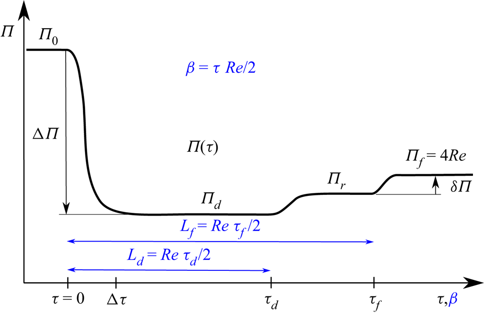
Figure 3. General pattern for complete laminarisation.
When the disturbance is over and the MPG has already experienced its main decrease,  $\varPi _d$, which causes the major deceleration in the U-ULF, the U-flow is left with a residual MPG $\varPi _r$, such that $\varPi _d\leq \varPi _r\leq \varPi _f=4Re$, and a U-ULF that is not yet coupled to the MPG and is still decreasing. This residual MPG is all that remains to definitely bring the U-ULF down to $Re(1-\alpha ^2)$; the lower $\varPi _r$ the faster the laminarisation, which occurs at time $\tau =\tau _f$, when the ULF reaches $\tilde {u}_L(\tau _f)=\varPi _f/8=Re/2$ and its bulk evolution ceases because it recouples with the MPG: the resulting flow would be completely laminarised, $\mathfrak {I}(\alpha )=1,\alpha \in (0,1)$ (see figure 3). This justifies calling $\tau _f$ the laminarisation time. The limit case $\varPi _r=\varPi _f$ would formally imply $\tau _f \rightarrow \infty$ and thus in practical applications one would expect $\varPi _r<\varPi _f$. The difference, $\delta \varPi =\varPi _f-\varPi _r$, will be called the excess MPG. If $\varPi _r>\varPi _f$ the ULF will never reach $\tilde {u}_L=Re/2$, the PTC will never be zero, and the flow will never laminarise completely, $\mathfrak {I}(\alpha )<1$ for some interval within (0,1). In this last case, $\tau _f$ would represent the time at which the bulk ULF no longer changes, and the name ‘laminarisation time’ would be somewhat uncalled for. Either way, we can define a length for laminarisation or a length for constant bulk ULF, given by $L_f= \tau _f \, Re /2$.
The account we have just offered will be called the laminarisation pattern, and we shall refer to it frequently. The notion that the MPG must be greatly reduced to attain complete laminarisation is central to understanding this mechanism, and the reader is strongly recommended to ponder over this idea prior to carry on reading. Note that  $Re_L(0)=Re_{L_0}=\varPi _0/4 \gg Re$ and $Re_L(\tau _f)=Re_{L_f}=\varPi _f/4=Re$. In figure 3 $\varPi _d$ has been depicted as roughly constant and generally would not be so; nevertheless, this fact should not alter the conclusions nor the mechanism for complete laminarisation described herein.
The reader would have noticed that no mention has been made of the PTC in the above explanation of the laminarisation pattern, despite the PTC being the component that encompasses the flow's turbulent motion. Otherwise put, we want  $\tilde {u}_T=0$ but no direct action is made over the RSSRG, which is the source of the PTC; instead, we act directly upon the MPG, which is the source of the ULF, a laminar flow. This apparent contradiction is solved by the condition $\tilde {u}_L+\tilde {u}_T=Re/2={\rm const}.$, (i), which constrains the U-flow: one acts upon the ULF to provoke a change in the PTC. The lower MPG can be considered a seed for complete laminarisation. Once the seed is planted, there is no way back; the U-flow will laminarise completely, it is just a matter of time. Figure 4 shows an imaginary example of the evolution of $\tilde {u}_L$ and $\tilde {u}_T$ for the case $\tilde {u} = \tau _f=1$. Note $\tilde {u}_L$ cannot decrease below $\tilde {u}=Re/2$. In mathematical terms, the U-flow has non-denumerable infinite ways of fulfilling the condition $\tilde {u}_L + \tilde {u}_T = Re / 2$; for each $\tilde {u}_L$ there is a unique $\tilde {u}_T$ but $\tilde {u}_L$ only responds to the MPG; reaching $\varPi _f=4 Re$ yields necessarily $\tilde {u}_L=\tilde {u}=Re/2$ and to this ULF corresponds uniquely the PTC $\tilde {u}_T=0$, i.e. a laminar flow.

Figure 4. Evolution of  $\tilde {u}_L$ and $\tilde {u}_T$ after a sufficiently low MPG (in arbitrary units, $\tilde {u}=\tau _f=1$). Each variation in $\tilde {u}_L$ must be matched by an equal and opposite variation in $\tilde {u}_T$.
Nevertheless, although the constraint  $\tilde {u}_L + \tilde {u}_T = Re / 2$ relieves us of studying the behaviour of the U-PTC, it is obvious that a vanishing PTC must be caused by a vanishing RSSRG, which is its source. From a mathematical standpoint, $\varSigma (\tau,\alpha ) \rightarrow 0$ could be caused either by a decaying turbulence, $\sigma (\tau,\alpha ) \rightarrow 0$, or by a homogeneous turbulence, because the latter also implies a zero radial gradient of RSS. Eventually, a turbulence forced to be homogeneous within a pipe, surrounded by walls, has just one possible outcome: the vanishing of turbulence, and this is what is observed in the experiments of Kuehnen et al. (Reference Kuehnen, Song, Scarselli, Budanur, Riedl, Willis, Avila and Hof2018b).
The laminarisation mechanism that has just been described is only possible with a constant  $Re$ during the U-flow evolution. Should changes in $Re$ be allowed, to achieve complete laminarisation it would also be necessary to act upon the PTC, i.e. to decrease its source, the RSSRG $\varSigma (\tau,\alpha )$. As was discussed in the previous paragraph, a convenient way to do it is to make the turbulence homogeneous throughout the pipe's cross-section, which irons out any gradient and vanishes the RSSRG. Curiously enough, usually it is necessary to very much increase the turbulence, so that it becomes uniformly high everywhere. Uniformly high or low, as long as it is homogeneous, in the end it will turn $\varSigma (\tau,\alpha )\approx 0$, leading to a negligible PTC, $\tilde {u}_T \approx 0$ (see § 6.2). Any turbulence that does not cause a radial gradient is irrelevant for the configuration of the mean-velocity field.
Whether  $\tilde {u}_T=0$ or not would depend upon how effective the disturbance has been (see figure 3); if successful, the U-flow would become laminar and would remain laminar forever, unless the disturbance were removed. Only a further disturbance that raises the MPG, or a relaxation of condition $Re={\rm const}.$, would provide some margin for the PTC to increase again. The laminarised S-flow would only undergo a transition to turbulence if its $Re$ is allowed to decrease (Mullin Reference Mullin2011). As a summary of the laminarisation pattern, we propose the following schematic sequence: steady state $\rightarrow$ local disturbance $\rightarrow$ very low $\varPi _d$ $\rightarrow$ ULF decoupled from MPG $\rightarrow$ end of disturbed domain $\rightarrow$ residual MPG $\varPi _r<\varPi _f$ $\rightarrow$ $\tilde {u}_L$ approaches $Re/2$ and $\tilde {u}_T$ approaches zero $\rightarrow$ ULF recouples to MPG $\rightarrow$ laminar Hagen–Poiseuille S-flow with $\varPi _f = 8 \tilde {u}_L=8 \tilde {u} = 4Re_L=4 Re$. Of course, the disturbance must be strong enough, and the disturbed domain long enough, for this sequence to unfold, and that constitutes one of the extraordinary merits of the experimental research of Kuehnen et al. (Reference Kuehnen, Song, Scarselli, Budanur, Riedl, Willis, Avila and Hof2018b). The account we have just exposed is the general picture the TULF offers to explain the observed phenomena.
The physico-mathematical problem, as modelled in figure 3, is thereby characterised by five degrees of freedom, namely,  $\varPi _d$ (or ${\rm \Delta} \varPi$), ${\rm \Delta} \tau$, $\tau _d$ (or $L_d$), $\varPi _r$ (or $\delta \varPi$) and $\tau _f$ (or $L_f$), which ought to be set in any experiment destabilising turbulence in pipe flow. Note $\varPi _0$ and $\varPi _f$ are determined by the initial conditions. The relationships among the energy input into the flow, $\varPi _d$, and $L_d$ will have to be found empirically in each case, as well as the residual MPG $\varPi _r$ beyond the perturbed domain. Arguably, the shorter $L_d$ the lower $\varPi _d$ to reach complete laminarisation, for a given energy-per-unit-length input. Most often, it would be necessary that $\varPi _d<0$ within the disturbed domain to attain complete laminarisation; otherwise put, the external energy supply would be converted into an adverse MPG. This surprising prediction will be explained in detail in § 6.3.
6.2. Four rotors experiment
We begin with the rotors experiment, which is the only one with a quasihomogeneous perturbation affecting the whole cross-section. The flow ( $Re=3500$) is vigorously stirred with four rotors, in pairs of clockwise and anticlockwise rotation. Kuehnen et al. (Reference Kuehnen, Song, Scarselli, Budanur, Riedl, Willis, Avila and Hof2018b) claim that the enhanced turbulence created by the rotors deforms the velocity profile, flattening it, and the deformation causes the U-flow to completely laminarise. Although we shall discuss later the flattening of U-profiles, what actually occurs in the experiment is the laminarisation pattern we exposed above, see figure 5. As anyone would imagine, both sources of mean motion, MPG $\varPi (\tau )$ and RSSRG $\varSigma (\tau,\alpha )$, play their role in the observed laminarisation. Thus, the moving rotors have two main effects in the U-flow, coinciding with both sources: (1) the rotors become an obstacle for the motion of the fluid and, as all obstacles do, they create a pressure drop in the U-flow, leading to a MPG decrease after starting the rotors, $\varPi _d<\varPi _0$ (see figure 5). (2) The rotors increase the turbulence around them, meaning that the fluctuating components of velocity $u'_i$, or the turbulence intensity $u'_i/\tilde {u}$, increase noticeably about the rotors. However, the newly created turbulence is uniform, homogeneous around the rotors and so is the associated RSS field. But a homogeneous RSS has a very small radial gradient, that is, $\varSigma (\tau,\alpha ) \approx 0$ and, since the RSSRG is the source of the PTC, we must expect a vanishing PTC or, otherwise put, a laminarised U-flow. An everywhere-increased turbulence is a likely route to laminarisation, for only the RSSRG constitutes a source of mean momentum. Any turbulence that does not cause a radial gradient is irrelevant for the configuration of the mean-velocity U-field; this is a very important outcome from the TULF (see (5.3) and (5.12)). Note the turbulence index field $\mathfrak {I}(\tau,\alpha )$ is not fooled by the uniform increase of turbulence intensity: in any laminarisation process $\mathfrak {I}(\tau,\alpha ) \rightarrow 1$ regardless of the turbulence intensity.

Figure 5. Sketch of MPG  $\varPi (\tau )$ evolution in the four rotors experiment (laminarisation pattern). Here $\varPi _L(\tau )$ is a virtual MPG, corresponding to the laminar Hagen–Poiseuille flow that at each instant has the same $Re_L$ as the U-ULF. (a) Successful complete laminarisation ( $\varPi _d =\varPi _r< \varPi _f=4Re$); (b) unsuccessful complete laminarisation ( $\varPi _d=\varPi _r > \varPi _f=4Re$).
No temporal evolution curves are offered for this experiment in Kuehnen et al. (Reference Kuehnen, Song, Scarselli, Budanur, Riedl, Willis, Avila and Hof2018b), and thus not much can be said about its degrees of freedom, except that the U-flow needs some  $130D$ to laminarise completely, $L_f=260$, according to Kuehnen et al. (Reference Kuehnen, Song, Scarselli, Budanur, Riedl, Willis, Avila and Hof2018b, supplementary figure 1). The antagonistic thrusts of the rotor pairs cause a large pressure drop in the U-flow, which can be adjusted to reach $\varPi _d< \varPi _f= 4 Re=14\,000$, although the relationship between rotor's spin velocity and $\varPi _d$ would have to be found empirically. The residual MPG $\varPi _r$ would be roughly the same as that created in the disturbed domain $\varPi _d$, and the situation in the U-flow could be described by ${\rm \Delta} \tau = \tau _d$ and $\varPi _d=\varPi _r$. With such low $\varPi _d$, since the U-flow's Reynolds number is not allowed to decrease, all available bulk velocity would be occupied by the ULF, and the PTC would be forced to zero (see point (2) above). Therefore, the final S-flow we must expect is a new ULF, devoid of PTC, with a Reynolds number $Re_{L}=Re=3500$, in accordance with the experiment (see figure 5a). No other explanation is required, but the simple and easily checkable pressure drop associated with any obstacle inserted in a flow. Regrettably, no results for the MPG are reported in the rotors experiment.
If the MPG decrease were not enough, then the residual ULF would have  $Re_{L_r}=2\tilde {u}_{L_r}>Re=2\tilde {u}$ and there would remain some residual bulk velocity available for a modest PTC, $\tilde {u}_{T_r}=\tilde {u}-\tilde {u}_{L_r}$: the laminarisation would not be complete and the final S-flow would be partially turbulent, with a greater turbulence index than that corresponding to the initial S-flow, $\mathfrak {I}_0(\alpha ) \leq \mathfrak {I}_r (\alpha ) \leq 1$ (see figure 5b).
Moreover, the laminarisation of a pipe flow would, in principle, be possible with any obstacle or device that could decrease sufficiently the MPG immediately downstream, like a honeycomb insert (Kuehnen, Scarselli & Hof Reference Kuehnen, Scarselli and Hof2019), an orifice plate (Kuehnen et al. Reference Kuehnen, Scarselli, Schaner and Hof2018a) or any other, while maintaining constant the U-flow's  $Re$.
$Re$.
The remaining experiments do depend on a definite disturbed-domain length  $L_d$, and the decrease of MPG is obtained through indirect methods (see §§ 6.3 and 6.4). We shall also see that the laminarisation pattern is only developed in the core flow, and an adverse MPG is generated therein. The external perturbation does not affect directly the whole cross-section, but rather the near-wall U-flow.
6.3. Annular streamwise jet experiment
The second experiment to be explained is the streamwise inject or annular jet ( $Re=5000$). Kuehnen et al. (Reference Kuehnen, Song, Scarselli, Budanur, Riedl, Willis, Avila and Hof2018b) claim that the WSS increases in the U-flow upon injecting the annular jet. This is literally true but not effectively true, for we must distinguish between flow and core flow, the latter being what remains after removing from the former the thin annular near-wall portion, see figure 6. Note this wall-adjacent annulus contains an inordinately high portion of the whole cross-sectional area.

Figure 6. Mean-velocity U-profile and sketch of dual MPG, strong favourable and moderate adverse, within the disturbed domain of the streamwise inject experiment.
The initial S-flow enters the disturbed domain with MPG  $\varPi _0$ and WSS $\sigma _{w_0}$, and the annular jet is input into the flow with moderately high velocity (we do not consider yet very high injection velocities, case $c4$ of Kuehnen et al. (Reference Kuehnen, Scarselli, Schaner and Hof2018a, figure 10b)), comparable to that of the core flow, and requires an external source of energy to do so. Therefore, the jet creates a sort of barrier between the core flow and the wall; the wall is shielded by the jet and loses contact with the core flow. The higher WSS becomes a private matter between wall and jet, not between wall and core flow. In the disturbed domain, figure 6, we see near the wall a strong favourable MPG that creates the jet itself, the accelerating wall flow, and also a lower (most often adverse) MPG in the core that decelerates the core flow, so that the constraint of fixed $Re$ could hold: if one portion of the U-flow accelerates then another must decelerate. Thus, the conditions to trigger the laminarisation pattern in the core flow are set, see figure 7. This local combination of favourable and adverse MPG in the same cross-sectional region is quite unstable, can only be sustained through an external energy input, cannot be maintained for long, and dissipates shortly downstream the disturbed domain, where the precarious cohabitation shown in figure 6 merges into a single MPG, the residual MPG $\varPi _r$ affecting the whole cross-section, which is the minimum found in Kuehnen et al. (Reference Kuehnen, Song, Scarselli, Budanur, Riedl, Willis, Avila and Hof2018b, figure 2a), measured some 30D downstream of the disturbed domain. Thereby, the actual occurrence of a dual MPG in the disturbed domain cannot be reproduced downstream, and instead an evolution curve with a single residual MPG is recorded. The account of facts just exposed is also substantiated in Kuehnen et al. (Reference Kuehnen, Scarselli, Schaner and Hof2018a, figure 12), which illustrates how the mean-velocity U-profiles evolve, with the wall flow swelling and the core flow shrinking as the energy input increases.

Figure 7. Laminarisation pattern: sketch of MPG  $\varPi (\tau )$ evolution in the core flow for the annular jet and radial jets experiments. Here $\varPi _L(\tau )$ is a virtual MPG, corresponding to the laminar Hagen–Poiseuille flow that at each instant has the same $Re_L$ as the U-ULF. (a) Successful complete laminarisation ( $\varPi _r < \varPi _f=4Re$); (b) unsuccessful complete laminarisation ( $\varPi _r > \varPi _f=4Re$).
Moreover, the velocity gradient between core flow and wall flow changes sign, see figure 6 and Kuehnen et al. (Reference Kuehnen, Scarselli, Schaner and Hof2018a, figure 12), and the disturbed domain can be defined as the region where this change of sign is present. The associated degree of freedom  $L_d$ would thus be given by the streamwise distance at which the dual MPG situation illustrated in figure 6 no longer holds. It is not a sharp and clear-cut definition, but it ought to suffice for designing experiments, and the relationship between injection velocity (or injection MPG) and $L_d$ would have to be found empirically. In a situation like this, in which the core flow is rather detached from the wall flow, (5.20) would also be approximately valid for the core flow, with $\varPi (\tau )$ the MPG acting upon the core flow (red line in figure 7). The core U-ULF is thus driven by a lower (most likely adverse) MPG and must decrease under its own dynamics, trailing the new MPG $\varPi _d$ (figure 7a), but any change in U-ULF must be accompanied by a matching one from U-PTC, (i). It follows that if $L_d$ and $\varPi _d$ are duly adjusted, the laminarisation pattern is initiated causing a laminarised core flow. If the wall flow is thin enough, it will contain just a small U-PTC, (vii), insufficient to ruin the core's laminarisation process if the merged residual MPG $\varPi _r$ is still well below $\varPi _f=4Re$. In this case, the initial core-flow laminarisation extends to the whole U-flow farther downstream. When the whole U-flow laminarises completely, the MPG increases again and recouples with the ULF, see figure 7(a) and Kuehnen et al. (Reference Kuehnen, Song, Scarselli, Budanur, Riedl, Willis, Avila and Hof2018b, figure 2a about $tU/D \approx 50$), but it will only increase up to $\varPi _f=4Re=20\,000$, whereby it becomes bulk stationary. The agent causing this late MPG increase is the force set in action by the constraint $Re={\rm const}.$ If, on the other hand, the residual MPG $\varPi _r > \varPi _f=4 Re$ then the associated U-ULF would be $\tilde {u}_{L_r}>Re/2=\tilde {u}$ and there would remain some residual U-PTC, $\tilde {u}_{T_r}=\tilde {u}-\tilde {u}_{L_r}$: the laminarisation would not be complete and the final S-flow would be partially turbulent, with a greater turbulence index than that corresponding to the initial S-flow, $\mathfrak {I}_0(\alpha ) \leq \mathfrak {I}_r (\alpha ) \leq 1$ (see figure 7b).
It remains to suggest an explanation for the case  $c4$ of Kuehnen et al. (Reference Kuehnen, Scarselli, Schaner and Hof2018a, figure 10b). Recall that, in figure 6, if $\delta \alpha = 1-1/\sqrt {2}\approx 0.2929$, then the area of the annulus containing the wall flow would be equal to that of the core flow. It is our belief that if the injection velocity is too high, the annular jet would not be so thin a few diameters downstream, and the core flow would not be dominant within the pipe's cross-section, see Kuehnen et al. (Reference Kuehnen, Scarselli, Schaner and Hof2018a, figure 12). Should this be the case, even if the core U-flow were to laminarise completely, there would remain a considerable U-PTC in the thicker annular jet itself that would prevent the complete laminarisation of the whole U-flow. Kuehnen et al. (Reference Kuehnen, Scarselli, Schaner and Hof2018a) even report that “ $\ldots$ meaning that the controlled flow exhibits features of relaminarisation but finally returns to a turbulent state downstream $\ldots$”. As long as the annular jet remains close to the wall, it will not develop a significant PTC, for the near-wall region is the natural domain of the ULF (García García & Fariñas Alvariño Reference García García and Fariñas Alvariño2019c), (vii).
6.4. Radial jets experiment
The last experiment to be discussed is that with 25 radial jets ( $Re=3100$). Again, in this flow we observe the same three performers on stage: jets; wall flow; and core flow. Of all quantities involved in the zero theorem for turbulent flow, (3.6), the one directly affected by the normal jets is the WSS $\sigma _w$. The jets change the WSS ‘felt’ by the core flow, see Kuehnen et al. (Reference Kuehnen, Song, Scarselli, Budanur, Riedl, Willis, Avila and Hof2018b, supplementary figure 6), since they create a barrier between wall and core flow: an external energy input is again detaching the core flow from the wall, and a new effective WSS appears in the core flow, $|\sigma _{w_d}|<|\sigma _{w_0}|$, and a new MPG is set in the disturbed domain, $\varPi _d=-2\sigma _{w_d}<\varPi _0$, (iii); thereby MPG and U-ULF decouple and the U-ULF is forced to pursue the new MPG $\varPi _d$ under its own dynamics, see figure 7. Again, we have the conditions that trigger the laminarisation pattern in the core flow. As discussed in § 6.3, in this situation (5.20) is approximately applicable to the core flow, with $\varPi (\tau )$ the resulting MPG after the disturbance (red line in figure 7). If $\tau _d$ is sufficiently long to render the effective WSS sufficiently low, the U-PTC within the core would fade off and the core U-flow would laminarise completely; in turn, its laminarisation would extend to the whole U-flow downstream, because the PTC is already negligible near the wall, (vii). The degree of freedom $L_d= \tau _d Re / 2$ is clearly set in this experiment of Kuehnen et al. (Reference Kuehnen, Song, Scarselli, Budanur, Riedl, Willis, Avila and Hof2018b), ${L_d=50}$, as opposed to the fuzzily defined $L_d$ of the previous annular streamwise-jet experiment. Downstream the disturbed domain, $\tau >\tau _d$, a residual MPG $\varPi _r$ remains in the U-flow (figure 7): if $\varPi _r \leq \varPi _f=4 Re$ the U-flow will eventually laminarise completely, otherwise a residual PTC would remain and the final S-flow would be partially turbulent, with a greater turbulence index than that corresponding to the initial S-flow, $\mathfrak {I}_0(\alpha ) \leq \mathfrak {I}_r (\alpha ) \leq 1$. The relationship between the injection velocity of radial jets and $\varPi _d$ would have to be found empirically.
6.5. Flattening of mean-velocity profiles
Kuehnen et al. (Reference Kuehnen, Song, Scarselli, Budanur, Riedl, Willis, Avila and Hof2018b) suggest repeatedly that the flattening of mean-velocity U-profiles might be the cause of the observed laminarisation, and even the experiments’ design appears to have been influenced by a pursuit of the said flattening effect. Linking the progress of laminarisation to a flattening of U-profiles is essentially correct, and is a testimony of those authors’ perspicacity. However, it is important to understand that the flattening is a consequence of the laminarisation process, not its cause. The flattening means, among other things, a deformation (change) of the mean-velocity field, and since Newton it is known that changes in momentum are caused by forces. Therefore, the flattening is caused by a modification of the forces applied to the U-flow, and only two forces are available: the MPG that pushes the U-flow; and the RSSRG that pulls in opposite direction, since it encompasses the turbulent stress forces. Moreover, the constraint of constant  $Re$ determines that both forces must be globally balanced at every instant, because the bulk acceleration is zero. However, they can differ locally, always provided the cross-section average of one be identical to the other, and the local differences tend to be greater near the wall, where the flattening manifests itself.
The defining characteristic of laminarisation is always a proportionally higher increase of the U-ULF respect to the U-PTC, hence its name. In any laminarisation process the U-ULF is proportionally greater than the U-PTC, and this occurs especially near the wall, where the U-PTC evolution is slower. Therefore, near the wall the subtracting term is lower in absolute value (the PTC is generally negative), and that yields a locally higher mean velocity, which is the observed phenomenon. The flattening of U-profiles is abundantly reported in our previous papers (García García & Fariñas Alvariño Reference García García and Fariñas Alvariño2019b,Reference García García and Fariñas Alvariñoc, Reference García García and Fariñas Alvariño2020, Reference García García and Fariñas Alvariño2021), and occurs every time the U-ULF takes precedence over the U-PTC, or otherwise put, any time the turbulence index increases. The mathematical details can be found in those references. All theoretical experiments we have performed in previous works show this effect: the route to laminarisation, either partial or total, implies the growth of the ratio  $|u_L/u_T|$, that is, the flattening of mean-velocity U-profiles.
We shall perform now a simple exercise to demonstrate that the deformation of mean-velocity U-profiles is a mathematical necessity in any U-flow evolution, as it follows from (5.12). The reader should note that, in the present context, ‘deformation’ means that the family of mathematical curves describing a U-flow is qualitatively different from that of a S-flow. Because of its simplicity, the informal demonstration will only be applied to the PresGrad component, (5.14), with an analogous reasoning for all other components. Assume a transient flow evolution from steady-state  $Re_1$ to steady-state $Re_2$. Since for horizontal S-flows the ULF and PresGrad are one and the same thing, the initial and final PresGrad components take the common form $\varPi _i (1-\alpha ^2)/4$ of a Hagen–Poiseuille flow. We begin by noting that the parabola function $1-\alpha ^2$ is expressed in Fourier–Bessel series as (see (7.16))
 \begin{equation} 1-\alpha^2 = 8 \sum _{n=1}^{\infty} \frac{J_0(\lambda_n \alpha )}{\lambda_n^3 J_1(\lambda_n)} = 4 \sqrt{2} \sum _{n=1}^{\infty} \frac{\phi_n(\alpha)}{\lambda_n^3}. \end{equation}
Let us imagine, just for a moment, that the PresGrad component were defined by
 \begin{equation} u_{P}(\tau,\alpha)=\sqrt{2} \left( \int _0^{\tau} \varPi(\tau') \, \mathrm{d} \tau' \right)\sum_{n=1}^{\infty} \frac{ \phi_n(\alpha)}{\lambda_n^3}, \end{equation}
with the integral over  $\varPi (\tau )$ outside of the sum, instead of the correct (5.14) (the extra $\lambda _n^2$ in the denominator arises from a change of variables in the integral of (5.14), $\xi ' = \lambda _n^2 \tau '$, $\mathrm {d} \tau ' = \mathrm {d} \xi '/\lambda _n^2$ and $\mathrm {e} ^{\xi -\xi '} \approx 1$). The integral would thus act as a global multiplicative factor of the parabola $(1-\alpha ^2)$. In this imaginary scenario, for each $\tau$ the U-profile of $u_P$ would be a parabola and the evolution of PresGrad would be a continuous sequence of parabolas up to the final one, $\varPi _2(1-\alpha ^2)/4$. Otherwise put, the temporal evolution of this component would be self-similar with respect to the variables $(\tau,\alpha )$. However, the correct mathematical result has the integral inside the sum, and the evolution U-profiles cannot be parabolas, but other curves that would appear as deformed when compared with a parabola. The particular form of such curves would depend on the disturbing factor within the sum, i.e. the integral over $\varPi$. The temporal evolution of PresGrad is not, and cannot be, self-similar with respect to $(\tau,\alpha )$, which is a pity because it would make life much easier. Arguably, the evolution of PresGrad could still be self-similar with respect to other variables, but that is a story to be told elsewhere. In summary, the deformation of mean-velocity U-profiles must occur in any temporal evolution of a U-flow; it is a prediction of the TULF and it is what actually happens in experiments.
7. Numerical data supporting explanations
Thus far we have described the general mechanisms to attain complete laminarisation, but no actual data has been offered. In this section we shall obtain some concrete numerical data that can be compared with those reported in Kuehnen et al. (Reference Kuehnen, Song, Scarselli, Budanur, Riedl, Willis, Avila and Hof2018b). The TULF requires an analytical model to perform the actual calculations that would yield the numerical results applicable to each experiment. By model we mean assigning concrete functions to the abstract quantities appearing in (5.12) and (5.20). We shall offer the analytical tools we normally employ in our research (García García & Fariñas Alvariño Reference García García and Fariñas Alvariño2019b,Reference García García and Fariñas Alvariñoc, Reference García García and Fariñas Alvariño2020, Reference García García and Fariñas Alvariño2021), and we shall apply them to the experiments encompassed in this study.
It is important to realise that laminarisation processes can be followed through the evolution of the laminar component alone, as was shown in § 6. The TULF yields the ULF component of any mean pipe flow and, therefore, the theory determines the mathematical constraints of momentum sources for laminarisation to occur. Recall the WSS is defined analytically by the ULF (see García García & Fariñas Alvariño Reference García García and Fariñas Alvariño2019c), and vice versa. This analytical relationship constitutes an additional insight into pipe flows, (García García & Fariñas Alvariño Reference García García and Fariñas Alvariño2019b,Reference García García and Fariñas Alvariñoc, Reference García García and Fariñas Alvariño2020, Reference García García and Fariñas Alvariño2021), and, eventually, deserves to be explored on laminarisation procedures.
7.1. A mathematical model for steady-state pipe flow
The following dimensionless polynomials (Pai Reference Pai1953), which we shall call a Pai flow, are a solution of the RANSE (3.2) and, therefore,  $u(\alpha )$ would correspond to the turbulent S-flow generated by the sources $\varPi$ and $\sigma (\alpha )$ in the natural normalisation,
 $$\begin{gather} u(\alpha)= \frac{\varPi}{4 \chi} \left( 1+\frac{\chi-q}{q-1} \alpha^2 - \frac{\chi-1}{q-1} \alpha^{2q} \right)= \frac{\varPi}{4}(1-\alpha^2)+ \frac{\hat{\varPi}}{4q} [ 1 - q(1-\alpha^2)-\alpha^{2q} ], \end{gather}$$
 $$\begin{gather}\sigma(\alpha)=\frac{\varPi}{2} \frac{q(\chi-1)}{\chi(q-1)}\alpha (1-\alpha^{2q-2})=\frac{\hat{\varPi}}{2} \alpha (1-\alpha^{2q-2} ), \end{gather}$$
with  $q\mathop {\geq }2$ a best-fitting integer and $\chi \in \mathbb {R}$, $1\mathop {\leq } \chi \mathop {<}q$, the so-called centreline turbulent dissipation (CTD), which is equal to the ratio
 \begin{equation} \chi = \frac{u_L(0)}{u(0)}=\frac{Re_L}{u(0)}=\frac{1}{\mathfrak{I}(0)}, \end{equation}
where  $u_L$ is the ULF generated directly by $\varPi$, i.e. a laminar Hagen–Poiseuille flow. According to its definition, $\chi =1$ for laminar flow, and in such case the value of $q$ is irrelevant. The functions $u(\alpha )$ and $\sigma (\alpha )$ thus defined belong to the mean space $\mathfrak {M}$ introduced in § 3. The first expression in (7.1) is called the compact form of a Pai flow, whereas the second is the decomposed form, for it shows explicitly the ULF ( $\varPi (1-\alpha ^2)/4$) and the PTC (the remainder). Note how $\hat {\varPi }=\varPi q (\chi -1)/\chi (q-1)$ plays in the PTC an analogous role to $\varPi$ in the ULF, and it is named the weighted MPG, being $\hat {\varPi } \lesssim \varPi$. The parameters $\varPi$, $q$ and $\chi$, which collectively characterise any Pai flow, are known as the spatial degrees of freedom (SDoF). These polynomials seem to have been largely ignored in the literature, despite representing quite accurately any turbulent S-flow of moderate $Re$. To assess the suitability of Pai polynomials, figure 8 compares the mean velocity of (7.1) with the experimental results of the Princeton Superpipe (see Zagarola Reference Zagarola1998), for the five lowest $Re$ of the set, which we name SP1 to SP5. The best-fitting SDoF parameters are given in table 1. We can see a small deviation in SP4, and a more noticeable one in SP5, albeit from SP1 to SP3 the coincidence is remarkable. In figure 9 is shown a Pai flow for $Re=5300$, together with the corresponding DNS data. This figure will be explained below.

Figure 8. Princeton Superpipe experimental velocity data and Pai polynomials for cases of table 1 (from García García & Fariñas Alvariño Reference García García and Fariñas Alvariño2019b).

Figure 9. The DNS velocity data for  $Re=5300$ in Wu & Moin (Reference Wu and Moin2008) and best-fitting Pai polynomial.
According to (3.3a,b),  $u(\alpha )$ and $\sigma (\alpha )$ determine each other uniquely; it follows that if (7.1) is a good approximation for the actual mean velocity, then (7.2) is also as good an approximation to the actual RSS. The plots of figure 2 have been calculated directly from the Pai polynomial (7.1) and the SDoF of table 1. It must be stressed, again, that Pai polynomials are a solution of the RANSE, (3.2), belonging to the mean space $\mathfrak {M}$, and not simply some functions presumed ad hoc (an example of an ad hoc mean-velocity profile would be the famous power law $u(\alpha )=u_{max}(1-\alpha )^{1/n}$, which does not fulfil the governing equation).
If we are just given a turbulent S-flow of Reynolds number  $Re$, and no further data, the SDoF can be obtained from the following expressions, which are as accurate as the correlations they emanate from, namely the Colebrook correlation and $u(0)= (1+1.3 \sqrt {f})\, \tilde {u}$, (see White Reference White2016, (6.43)). The demonstration is given in Appendix B:
 $$\begin{gather} \varPi=\frac{f\, Re^2}{16}, \end{gather}$$
 $$\begin{gather}\chi_1=\frac{f\, Re}{32(1+1.3 \sqrt{f})}, \end{gather}$$
 $$\begin{gather}q_1=\frac{\chi_1 (f \, Re-64)}{64 \chi_1 - f \, Re}, \end{gather}$$
((7.4) was also deduced in Marusic et al. (Reference Marusic, Joseph and Mahesh2007, (4.1))). Equation (7.6) will not generally yield an integer value for  $q_1$. In that case, we round $q_1$ to the nearest integer $q\in \mathbb {N}$, always provided $q>\chi _1$, and we reckon a new $\chi$ from the following equation:
 \begin{equation} \chi=\frac{q\ f\, Re}{64(q+1)-f\, Re}. \end{equation}
Moreover, we have the interesting relationship,
 \begin{equation} f\, Re = 64\frac{\chi (q+1)}{\chi+q}, \end{equation}
which is exactly  $f\, Re = 64$ for laminar flow ( $\chi =1$), regardless of the value of $q$.
$q$.
The bulk velocity corresponding to a Pai flow, (7.1), is
 \begin{equation} \tilde{u}= \tilde{u}_L + \tilde{u}_T = \frac{\varPi}{8} - \frac{\hat{\varPi}}{8} \frac{q-1}{q+1}= \frac{\varPi}{8} \frac{\chi+q}{\chi(q+1)} = \frac{Re}{2}. \end{equation}
Note that if  $q> \chi \gg 1$, then $\hat {\varPi } \approx \varPi$, $\tilde {u}_L \approx |\tilde {u}_T|$ and $\tilde {u} \ll \tilde {u}_L$, which is the result depicted in figure 2. The bulk velocity $\tilde {u}$ is usually a dwarf compared with those two giants, $\tilde {u}_L$ and $\tilde {u}_T$.
Given a turbulent S-flow with bulk velocity  $\tilde {u}$, the laminar Hagen–Poiseuille flow with the same bulk velocity satisfies $\tilde {u}=\tilde {u}_L=\varPi _f/8$ (see (2.8)), whereby the MPG of the laminar flow must fulfil (see (7.9))
 \begin{equation} \varPi_f=\varPi \frac{\chi+q}{\chi(q+1)} , \quad \varPi_f<\varPi. \end{equation}
 To assess how accurate the Pai polynomial resulting from the above procedure is, we shall apply it now to the DNS flow of  $Re=5300$ obtained in Wu & Moin (Reference Wu and Moin2008), which has a Reynolds number within the order of magnitude of those reported in Kuehnen et al. (Reference Kuehnen, Song, Scarselli, Budanur, Riedl, Willis, Avila and Hof2018b). Applying (7.4)–(7.7) to $Re=5300$, we obtain $f=0.03677$, $\varPi =64560.46$, $\chi _1=4.87524$ and $q_1=5.44901$. Rounding $q_1$ to $q=6$, we get $\chi =4.62029$. The DNS data of Wu & Moin (Reference Wu and Moin2008) is furnished in wall units, $u^+=U/U_{\tau }$. To convert wall units into the natural normalisation, suffices to apply $u=u^+ \, Re_{\tau }$, being $Re_{\tau }=U_{\tau } R /\nu$ the friction Reynolds number, also called the von Kármán number. For the chosen DNS flow, it is $Re_{\tau }=181.37$. The resulting Pai polynomial is plotted in figure 9, together with the DNS velocity data. The DNS data appear to have been time-averaged rather than ensemble-averaged (see Wu & Moin Reference Wu and Moin2008, § 2.3), whereas the Pai flow is always a mathematically ensemble-averaged field. A slightly better fit would have been obtained if $q$ were allowed to have non-integer values. However, in such case the solution would not be a polynomial, and much of the analytical advantage would be lost.
The case of a turbulent Hagen–Poiseuille flow with MPG  $\varPi$ and moving-wall velocity $V_w$ is somewhat more involved. Recall we mentioned in § 4 that given a turbulent Hagen–Poiseuille–Couette flow $u(\alpha )$, the field $u_w(\alpha ) \equiv u(\alpha )-V_w$ corresponds mathematically to a turbulent Hagen–Poiseuille flow with the same sources, $\varPi$ and $\sigma (\alpha )$. We shall now use this result to characterise a turbulent Hagen–Poiseuille–Couette flow through polynomials. The mean-velocity field is (see (4.2a,b))
 \begin{align} u(\alpha)&=V_w+ \frac{\varPi}{4 \chi_w} \left( 1+\frac{\chi_w-q}{q-1} \alpha^2 - \frac{\chi_w-1}{q-1} \, \alpha^{2q} \right) \nonumber\\ &= V_w+\frac{\varPi}{4}(1-\alpha^2)+ \frac{\check{\varPi}}{4q} [ 1 - q(1-\alpha^2)-\alpha^{2q} ], \end{align}
in which  $q$ is, again, a best-fitting integer, but $\chi _w$ now responds to
 \begin{equation} \chi_w=\frac{u_{w_L}(0)}{u_w(0)}=\frac{u_L(0)-V_w}{u(0)-V_w}, \end{equation}
according to the definition of CTD  $\chi$ offered above for turbulent Hagen–Poiseuille flow. Likewise, the Couette-weighted MPG $\check {\varPi }$ is defined by
 \begin{equation} \check{\varPi}=\varPi \frac{q(\chi_w-1)}{\chi_w(q-1)}. \end{equation}
Thereby, if we are only given a turbulent Hagen–Poiseuille–Couette flow characterised by  $Re$ and $V_w$, then we calculate $Re_w=Re-2V_w$ (see (3.12) and (4.5)), and with $Re_w$ we reckon $f_w$ through the Colebrook correlation, and now we can apply the set of (7.4)–(7.7) to determine the SDoF parameters defining $u_w(\alpha )$ and (7.11): $\varPi$, $\chi _w$ and $q$. The bulk velocity of a turbulent Hagen–Poiseuille–Couette flow is
 \begin{equation} \tilde{u}= \tilde{u}_L + \tilde{u}_T = V_w +\frac{\varPi}{8} - \frac{\check{\varPi}}{8} \frac{q-1}{q+1}= V_w+\frac{\varPi}{8} \frac{\chi_w+q}{\chi_w(q+1)} =\frac{Re}{2}. \end{equation}
7.2. A mathematical model for transient pipe flow
As already explained in § 5, defining a model within the framework of the TULF means assigning explicit mathematical functions to the abstract quantities  $\varPi (\tau )$, $\varGamma (\tau )$, $\varSigma (\tau,\alpha )$, $V_w(\tau )$ and $u_0(\alpha )$ appearing in (5.12) and (5.20). When applied to the experiments of Kuehnen et al. (Reference Kuehnen, Song, Scarselli, Budanur, Riedl, Willis, Avila and Hof2018b), (5.12) and (5.20) become greatly simplified, for ${\varGamma (\tau )=V_w(\tau )=0}$. Moreover, we are not concerned about the particular details of mean-velocity U-profiles, and thus we can work only with bulk velocities and (5.20). Last, but by no means least, the constraint $\tilde {u}_L(\tau )+\tilde {u}_T(\tau )=Re/2$, (i), allows us to study exclusively the evolution of the U-ULF $\tilde {u}_L(\tau )$, and we are thereby spared the burden of finding suitable functions $\varSigma (\tau,\alpha )$ for these flows. Therefore, the bulk U-ULF applicable in this research is limited to (see (5.20))
 \begin{equation} \tilde{u}_L(\tau)=4 \sum _{n=1}^{\infty} \left\{ \frac{u_{L_n}^{(0)}}{\sqrt{2}} \frac{\mathrm{e}^{-\lambda_n^2 \tau}}{\lambda_n} + \frac{1}{\lambda_n^2} \int _0^{\tau} \varPi(\tau')\, \mathrm{e}^{-\lambda_n^2 (\tau-\tau')} \, \mathrm{d}\tau' \right\}. \end{equation}
Since the initial flow in all experiments is a turbulent S-flow as in (3.3a,b), its corresponding S-ULF is the Hagen–Poiseuille flow  $u_{0_L}(\alpha )=\varPi _0 (1-\alpha ^2)/4$.The components of $u_{0_L}(\alpha )$ in the basis $\{\phi _n(\alpha ) \}$ of the Hilbert space $L^2_{\alpha }(0,1)$ are given by the inner product
 \begin{equation} u^{(0)}_{L_n}=\left\langle \frac{\varPi_0}{4}(1-\alpha^2),\phi_n(\alpha) \right\rangle= \frac{\varPi_0}{4}\int _0^1 \alpha (1-\alpha^2) \frac{\sqrt{2} \ J_0(\lambda_n \alpha)}{J_1(\lambda_n)} \, \mathrm{d} \alpha= \frac{\sqrt{2}\ \varPi_0}{\lambda_n^3}, \end{equation}
and (7.15) is written as
 \begin{equation} \tilde{u}_L(\tau)=4 \sum _{n=1}^{\infty} \frac{ \mathrm{e}^{-\lambda_n^2 \tau}}{\lambda_n^2} \left\{ \frac{\varPi_0 }{\lambda_n^2} + \int _0^{\tau} \varPi(\tau')\, \mathrm{e}^{\lambda_n^2 \tau'} \, \mathrm{d}\tau' \right\}. \end{equation}
It remains to find an expression for the MPG  $\varPi (\tau )$. The actual MPG might be a rather complicated function, but in figure 3 we offered a likely model and in § 6.1 it was reduced to defining five degrees of freedom ( $\varPi _d$, ${\rm \Delta} \tau$, $\tau _d$, $\varPi _r$ and $\tau _f$), because $\varPi _0$ and $\varPi _f$, the initial and final MPG, are uniquely determined by $Re$. Unfortunately, the data reported in Kuehnen et al. (Reference Kuehnen, Song, Scarselli, Budanur, Riedl, Willis, Avila and Hof2018b) for any of the experiments are not sufficient to uniquely fix those five parameters, and there are infinitely many possibilities for them. Therefore, we shall devise a much-simplified model for $\varPi (\tau )$ and assume that the MPG drops instantaneously to $\varPi _d$, and stays there until complete laminarisation is attained, i.e. $\varPi _r=\varPi _d$ and ${\rm \Delta} \tau = \tau _d=0$. The model is purposely chosen to be very simple, so that no doubt remains that the final outcome (a laminar S-flow) is predicted even with a low-accuracy model. We are left with only two degrees of freedom, $\varPi _d=\varPi _r$ and $\tau _f$. This simplifying assumption is based upon (iv) and mathematically can be formulated as the MPG following a Heaviside step ${\rm \Delta} \varPi$ at dimensionless time $\tau =0$,
 \begin{equation} \varPi(\tau)= \varPi_0 +{\rm \Delta} \varPi \mathcal{H}(\tau) = \varPi_0 + (\varPi_d-\varPi_0)\mathcal{H}(\tau), \end{equation}
with  $\mathcal {H}(\tau )$ the Heaviside unit distribution. Under such an assumption and inserting this $\varPi (\tau )$ into (7.17), the TULF provides the following continuous function for a fully developed $\tilde {u}_L(\tau )$ that attains complete laminarisation at $\tau _f$ ( $\varPi _r<\varPi _f=4 Re$):
 \begin{equation}
\tilde{u}_L(\tau)=\begin{cases} \displaystyle 4 \sum
_{n=1}^{\infty}\frac{\varPi_0 \, \mathrm{e}^{-\lambda_n^2
\tau} + \varPi_d(1-\mathrm{e}^{-\lambda_n^2
\tau})}{\lambda_n^4}\\
\qquad =\frac{\varPi_d}{8}-4 {\rm \Delta} \varPi
\sum _{n=1}^{\infty}
\frac{\mathrm{e}^{-\lambda_n^2\tau}}{\lambda_n^4}
=\frac{\varPi_L(\tau)}{8} & 0\leq \tau \leq \tau_f ,\\
\displaystyle \frac{Re}{2}=\frac{\varPi_f}{8} & \tau >
\tau_f. \\ \end{cases}
\end{equation}
\begin{equation}
\tilde{u}_L(\tau)=\begin{cases} \displaystyle 4 \sum
_{n=1}^{\infty}\frac{\varPi_0 \, \mathrm{e}^{-\lambda_n^2
\tau} + \varPi_d(1-\mathrm{e}^{-\lambda_n^2
\tau})}{\lambda_n^4}\\
\qquad =\frac{\varPi_d}{8}-4 {\rm \Delta} \varPi
\sum _{n=1}^{\infty}
\frac{\mathrm{e}^{-\lambda_n^2\tau}}{\lambda_n^4}
=\frac{\varPi_L(\tau)}{8} & 0\leq \tau \leq \tau_f ,\\
\displaystyle \frac{Re}{2}=\frac{\varPi_f}{8} & \tau >
\tau_f. \\ \end{cases}
\end{equation}
If, on the other hand, complete laminarisation is not reached ( $\varPi _r>\varPi _f=4 Re$), the bulk U-ULF takes the form
 \begin{equation} \tilde{u}_L(\tau)= 4 \sum _{n=1}^{\infty}\frac{\varPi_0 \, \mathrm{e}^{-\lambda_n^2 \tau} + \varPi_d(1-\mathrm{e}^{-\lambda_n^2 \tau})}{\lambda_n^4}=\frac{\varPi_d}{8}-4 {\rm \Delta} \varPi \sum _{n=1}^{\infty} \frac{\mathrm{e}^{-\lambda_n^2\tau}}{\lambda_n^4} =\frac{\varPi_L(\tau)}{8}. \end{equation}
Note that at  $\tau =0$ only the terms with $\varPi _0$ survive, whereas for $\tau \rightarrow \tau _f$, (7.19) (respectively for $\tau \rightarrow \infty$, (7.20)) only the terms with $\varPi _f/8$ (respectively, $\varPi _d/8$) remain. In the meantime, $\tilde {u}_L(\tau )$ would be equal to the bulk velocity of a laminar Hagen–Poiseuille flow driven by an intermediate virtual MPG $\varPi _L(\tau )$, $u^S(\alpha ;\tau )=\varPi _L(\tau ) (1-\alpha ^2 )/4$, see (viii), although $\varPi _d$ be already enforced downstream of the disturbed domain. The MPG corresponding to this virtual SB-flow, $\varPi _L(\tau )$, is represented in green colour in figures 5 and 7. The excess MPG, $\delta \varPi = \varPi _f-\varPi _r=\varPi _f-\varPi _d$, needed by the U-flow to reach $\varPi _f$ within a finite time interval, will be recovered once the ULF has attained $\tilde {u}_L=Re/2$ (see red lines in figures 5a and 7a). If, on the contrary, $\varPi _r>\varPi _f$, then the ULF will be limited by $\tilde {u}_L \rightarrow \varPi _d/8=\varPi _r/8>Re/2$, and the difference $\tilde {u}_T=Re/2 - \tilde {u}_L$ would correspond to the S-PTC, which would not be zero and the flow would not laminarise completely. This last situation is illustrated in figures 5b and 7b. In any case, $\tau _f$ denotes the time at which the ULF does not measurably change, either because it has reached $Re/2$ with an excess MPG $\delta \varPi >0$, or because it is asymptotically arriving to $\varPi _r/8=\varPi _d/8$ and there is no significant MPG to drive the ULF any lower ( $\delta \varPi <0$). This account of facts, based upon (7.19) and (7.20), constitutes, again, the laminarisation pattern introduced above.
Let us forget for the moment the unsuccessful case. If the experiment is successful and a complete laminarisation is attained, then from (7.19) it follows that
 \begin{align} \sum _{n=1}^{\infty} \frac{\mathrm{e}^{-\lambda_n^2\tau_f}}{\lambda_n^4} &=\frac{\varPi_d-4Re}{32(\varPi_d-\varPi_0)} =\frac{-\delta \varPi}{32 {\rm \Delta} \varPi}\nonumber\\ &\Leftrightarrow \varPi_d=\left( 32 \varPi_0 \sum _{n=1}^{\infty} \frac{\mathrm{e}^{-\lambda_n^2\tau_f}}{\lambda_n^4}-4Re \right) \left( 32 \sum _{n=1}^{\infty} \frac{\mathrm{e}^{-\lambda_n^2 \tau_f}}{\lambda_n^4} - 1 \right)^{{-}1}, \end{align}
which relates  $\varPi _d$ and $\tau _f$ for the initial S-flow defined by $Re$ and $\varPi _0$. If $\tau _f$ is known, $\varPi _d$ can be reckoned rather easily with the equation on the right-hand side, for the series converges rapidly and is quite accurate with some 50 terms or fewer. If, instead, $\varPi _d$ is known, the equation on the left-hand side can be solved recursively, starting with an estimated value for $\tau _f$. With the first eigenvalue $\lambda _1 \approx 2.404826$ being the most significant of the series, it is a smart idea to begin the recursion with $\tau _{f_1}$ given by
 \begin{equation} \frac{\mathrm{e}^{-\lambda_1^2\tau_{f_1}}}{\lambda_1^4} = \frac{\varPi_d-4Re}{32(\varPi_d-\varPi_0)} \Rightarrow \tau_{f_1} = \frac{-1}{\lambda_1^2} \ln \left[\frac{\lambda_1^4 (\varPi_d-4Re)}{32(\varPi_d-\varPi_0)} \right]= \frac{-1}{\lambda_1^2} \ln \left[ \frac{-\lambda_1^4 \delta \varPi}{32 {\rm \Delta} \varPi} \right], \end{equation}
knowing that, typically,  $\tau _{f_1}$ yielded by (7.22) is rather similar to the actual $\tau _f$, i.e. $\tau _{f_1} \sim \tau _f$ ( $\delta \varPi \geq 0$, ${\rm \Delta} \varPi <0$, and $\delta \varPi <|{\rm \Delta} \varPi |$). On the other hand, if $\tau _{f_1}$ defined by (7.22) were good enough to design an experiment, the researcher would not need to write the software that calculates (7.21). Finally, should higher accuracy be needed, the reader can always devise a more sophisticated model for $\varPi (\tau )$ than (7.18) (figure 3 might serve as guide).
To end this section, and as a concomitant of the solution just found, we shall reckon the time constant of the dynamical system constituted by a laminar pipe U-flow. To our knowledge, the consideration of a laminar flow as a dynamical system, and thus liable of having time constant, phase space, orbits, Lyapunov exponents and like notions, is not frequently reported in the literature, and might be of interest to the reader. For an energy-increasing system, such a time constant  $\tau _c$ is defined as the time needed for the dynamical system to yield the value $\tilde {u}_L(\tau _c) \equiv (1-\mathrm {e}^{-1}) \tilde {u}_L(\infty ) \approx 0.6321 \tilde {u}_L(\infty )$, where $\tilde {u}_L(\infty )$ is the limit steady-state response obtained after applying a unit Heaviside step at $\tau =0$ in the system's source. For an energy-decreasing system, it would be $\tilde {u}_L(\tau _c) \equiv \mathrm {e}^{-1} \tilde {u}_L(\infty ) \approx 0.3679 \tilde {u}_L(\infty )$. Applied to our case, we assume that the MPG (the source) undergoes a unit Heaviside step from $\varPi _0$ to $\varPi _0+1$ at $\tau =0$, i.e. (7.18) would become $\varPi (\tau )=\varPi _0+\mathcal {H}(\tau )$, since $\varPi _d=\varPi _0+1$ and ${\rm \Delta} \varPi =1$. The equation defining the time constant $\tau _c$ can either be derived from (7.19) or (7.20), as follows:
 \begin{equation} \tilde{u}_L(\tau_c)=\frac{\varPi_0}{8}+(1-\mathrm{e}^{{-}1})\frac{1}{8}= \frac{\varPi_0+1}{8}- 4 \sum_{n=1}^{\infty} \frac{\mathrm{e}^{\lambda_n^2 \tau_c}}{\lambda_n^4} \Rightarrow \sum _{n=1}^{\infty} \frac{\mathrm{e}^{(1-\lambda_n^2\tau_c)}}{\lambda_n^4}=\frac{1}{32}. \end{equation}
This is an extremely interesting result: the time constant  $\tau _c$ does not depend upon the Reynolds number of the laminar flow (or the MPG $\varPi _0$, which is the same thing). Moreover, the same result is obtained if, instead of a unit Heaviside step ( ${\rm \Delta} \varPi =1$), a general Heaviside step ${\rm \Delta} \varPi$ is applied to the flow. Here $\tau _c$ seems to be a universal constant, valid for any laminar pipe flow. Since $\tau _c=t_c \nu /R^2$, it should be stated that the dimensional time constant $t_c$ depends exclusively upon the fluid's viscosity and the pipe's radius. The response of a laminar flow to any step increase in MPG is the same for all initial bulk velocities of such a flow or, otherwise put, for given pipe and fluid the time constant of a laminar flow is the same for all $Re$. Moreover, the reader should be aware of the following identity involving the zeros $\lambda _n$ of $J_0(x)$:
 \begin{equation} \sum _{n=1}^{\infty} \frac{1}{\lambda_n^4}=\frac{1}{32}, \end{equation}
which helps one understand the relevance of (7.23). Reckoning the series (7.23) with 500 terms, we get for the universal time constant the value
 \begin{equation} \tau_c= \frac{t_c \nu}{R^2} = 0.165381775. \end{equation}
 Future experimental research should take into account this universal time constant; to get a swift laminarisation (or any other unsteady effect), one should use small-diameter pipes and high-viscosity fluids. Be warned that it is not a matter of Reynolds number, since the bulk velocity plays no role in how fast the flow reacts to any perturbation. This advice also serves to minimise the necessary disturbed-domain size to attain complete laminarisation. The dimensionless length corresponding to  $\tau _c$ is $L_c=\tau _c Re/2$ (see (6.1)). As $\tau _c$ is constant, we have the result $L_c \propto Re$ (dimensionless) or L $_c \propto R\ Re$ (dimensional). In both cases, we arrive at the conclusion that the “development length required to reach a fully parabolic profile increases linearly with $Re$”, as expressed literally in Kuehnen et al. (Reference Kuehnen, Song, Scarselli, Budanur, Riedl, Willis, Avila and Hof2018b, caption of figure 3b).
7.3. Four rotors experiment
We begin with the four rotors experiment,  $Re=3500$. With such a $Re$, (7.4)–(7.10) yield $f=0.041528$, $\varPi _0=31795$, $q=4$ and $\chi =3.328906$. The final MPG to attain complete laminarisation is $\varPi _f=14\,000$, according to (7.10). At 18 $^\circ$C, the kinematic viscosity of water is $\nu =1.0533 \times 10^{-6} \ {\rm m}^2\ {\rm s}^{-1}$, and as $D=2R=54 \ {\rm mm}$ for this experiment, we have $\tilde {U}=0.06827 \ {\rm m}\ {\rm s}^{-1}$ ( $\tilde {u}=1750$). Since the flow is reported to laminarise completely at some $130D$ downstream ( $L_f \approx 260$), we can estimate $\tau _f= L_f/\tilde {u} \approx 0.14857$, i.e. $t_f \approx 102.83\ {\rm s}$. Thereby, according to (7.21) with 50 terms in the series, we have $\varPi _d=\varPi _r=1858.7652$, a low favourable MPG. No adverse MPG is necessary in this case to attain complete laminarisation. Additionally, the MPG drop in the disturbed domain is ${\rm \Delta} \varPi = \varPi _d-\varPi _0=-29937.24$, and the excess MPG recovered at complete laminarisation ( $\tilde {u}_T(\tau _f)=0$) is $\delta \varPi = \varPi _f-\varPi _r=12141.24$ (see laminarisation pattern in figure 5). Note $\tau _f$ is slightly below the universal time constant $\tau _c$ of (7.25), $\tau _f \lesssim \tau _c$, which means that the final laminar Hagen–Poiseuille flow is attained later, as already reported in Kuehnen et al. (Reference Kuehnen, Song, Scarselli, Budanur, Riedl, Willis, Avila and Hof2018b, caption in figure 3b); that is, the mean flow is laminar for $\tau > \tau _f$, but it is still a U-flow with a not-yet parabolic profile shortly after $\tau _f$ (see § 6.5). We shall use the ratio $|{\rm \Delta} \varPi | / \varPi _0$ as a figure of merit to assess how significant the MPG decrement is to achieve complete laminarisation within the requested time interval. This ratio gives information about how effective the laminarisation method is to rapidly accomplish the desired result. In the rotors experiment it is $|{\rm \Delta} \varPi | / \varPi _0=0.9416$.
7.4. Annular streamwise jet experiment
Let us now examine the annular jet experiment, whose results are reported in Kuehnen et al. (Reference Kuehnen, Song, Scarselli, Budanur, Riedl, Willis, Avila and Hof2018b, figure 2a), which correspond to measurements made far downstream the disturbed domain, where the U-flow is fully developed. With  $Re=5000$, (7.4)–(7.10) yield $f=0.037393$, $\varPi _0=58426$, $q=5$, $\chi =4.7444$, $\tilde {u}=Re/2=2500$ and $\varPi _f=4Re=20\,000$. Note that $\varPi _0/\varPi _f=2.9213$, which is approximately the result reported by Kuehnen et al. (Reference Kuehnen, Song, Scarselli, Budanur, Riedl, Willis, Avila and Hof2018b), “ $\ldots$ by a factor of 2.9 (see Fig. 2a) $\ldots$”. Inside the disturbed domain the situation is analogous to figure 6, with a dual MPG; however, at the measurement station the dual MPG cannot be recorded, as they merge into a single MPG. The instant at which the MPG begins to increase can be identified with the laminarisation time, $\tau _f$, see figure 7(a), and $\tau _f$ can be measured directly on Kuehnen et al. (Reference Kuehnen, Song, Scarselli, Budanur, Riedl, Willis, Avila and Hof2018b, figure 2a), yielding $t_f^* = t_f \tilde {U}/D \approx 35$ dimensionless time units. With $\tilde {u}=2500$, $D=2R=0.03 \ {\rm m}$ and $\nu =1.0533 \times 10^{-6} \ {\rm m}^2\ {\rm s}^{-1}$, we have a dimensional bulk velocity $\tilde {U}\approx 0.17555 \ {\rm m}\ {\rm s}^{-1}$. Therefore, a time unit in Kuehnen et al. (Reference Kuehnen, Song, Scarselli, Budanur, Riedl, Willis, Avila and Hof2018b, figure 2a) is equivalent to $D/\tilde {U}=0.171 \ {\rm s}$, and the laminarisation time would be $t_f \approx 6 \ {\rm s}$, which in the natural normalisation, (2.3a–c), corresponds to dimensionless time $\tau _f = t_f \nu /R^2 = 0.0281$. The corresponding laminarisation length would be $L_f= \tilde {u} \tau _f\approx 70$, or $35D$, which is quite close to the $30D$ distance reported in the actual experiment (Kuehnen et al. Reference Kuehnen, Song, Scarselli, Budanur, Riedl, Willis, Avila and Hof2018b). With these values, (7.21) applied to the core flow yields $\varPi _d=-165825.9642$ using 50 terms in the series, and $\varPi _d=-165825.9229$ with only five terms; the error is negligible, for the series converges very fast. Using, instead, (7.22) with $\tau _{f_1}=0.0281$, we obtain $\varPi _d=-147367.64$, with an error of $11.13\,\%$. Either way, the effect of the annular jet upon the core flow is an adverse MPG: the jet itself causes a brusque acceleration in the wall flow, but since the flow's $Re$ is not allowed to change, the core flow must decelerate (through an adverse MPG) to compensate for. The result is not so surprising, if we consider how much energy the turbulence dissipates from the flow, see figure 2; it is only natural that a powerful disturbance be needed to eliminate the turbulence. Obviously, the adverse MPG is only active within the disturbed domain; farther downstream of the disturbed domain, where the U-flow is fully developed, the dual MPG merges into a residual MPG $\varPi _r$ that is transmitted and recorded, and this is what Kuehnen et al. (Reference Kuehnen, Song, Scarselli, Budanur, Riedl, Willis, Avila and Hof2018b, figure 2a) shows. In this experiment $\tau _f \ll \tau _c$, with $\tau _c$ given by (7.25), which implies the final laminar Hagen–Poiseuille flow is reached much later, as reported in Kuehnen et al. (Reference Kuehnen, Song, Scarselli, Budanur, Riedl, Willis, Avila and Hof2018b, caption in figure 3b). Shortly after $\tau _f$ the flow is laminar, but it has a mean-velocity U-profile that is far from being a parabola (see § 6.5). The figure of merit for this experiment, in the core flow, is $|{\rm \Delta} \varPi | / \varPi _0=3.8382$, and complete laminarisation is accomplished much sooner than in the rotors experiment.
7.5. The 25 radial jets experiment
Finally, we study the 25 radial jets experiment,  $Re=3100$. Equations (7.4)–(7.10) yield $f=0.0430845$, $\varPi _0=25878$, $q=4$, $\chi =2.8656$, $\tilde {u}=1550$ and $\varPi _f=12\ 400$. According to (7.1), the centreline mean velocity is $u(0)=\varPi _0/4\chi =2257.64$, and the ratio between $u(0)$ and the bulk velocity $\tilde {u}=Re/2$ is $2u(0)/Re \approx 1.46$, which is coincident with the average value shown in Kuehnen et al. (Reference Kuehnen, Song, Scarselli, Budanur, Riedl, Willis, Avila and Hof2018b, figure 1d, bottom panel). The disturbed domain is characterised by $L_d=50$ and $\tau _d = 2 L_d/ Re =0.03226$, whereas $\tilde {U}=0.10884\ {\rm m}\ {\rm s}^{-1}$ as calculated from $\nu =1.0533 \times 10^{-6} \ {\rm m}^2\ {\rm s}^{-1}$ and $D=2R=0.03\ {\rm m}$. Measuring directly over Kuehnen et al. (Reference Kuehnen, Song, Scarselli, Budanur, Riedl, Willis, Avila and Hof2018b, figure 1d, top panel), we see that the transient flow begins at approximately $t_1^*=t_1 \tilde {U}/D \approx 28.1$ (corresponding to $\tau =0$), and ends at $t_2^*=t_2 \tilde {U}/D \approx 35.7$ (corresponding to $\tau _f$), thus yielding $t^*_f=t_2^*-t_1^* \approx 7.6$, which in the natural normalisation is $\tau _f \approx 0.009807$. With such data, (7.21) applied to the core flow yields $\varPi _d=-174814.42$ with 50 terms in the series. No wonder that $\varPi _d$ is a strong adverse MPG, if we have into account that $\tau _f = 0.009807$ is over three times lower than $\tau _d = 0.03226$ (or $L_d \approx 3.3 L_f$), that is, the U-flow is completely laminarised before exiting the disturbed domain, see figure 10. Apparently, the radial jets set-up is a very compelling technique for laminarisation. Therefore, $\tau _f \ll \tau _c$ for this experiment, $\tau _c$ defined in (7.25), from which follows that the final parabolic laminar Hagen–Poiseuille flow is achieved much later, in accordance with Kuehnen et al. (Reference Kuehnen, Song, Scarselli, Budanur, Riedl, Willis, Avila and Hof2018b, caption in figure 3b). The figure of merit for this experiment is $|{\rm \Delta} \varPi | / \varPi _0=7.7553$, the highest of them all.

Figure 10. Sketch of MPG  $\varPi (\tau )$ evolution in the core flow for the 25 radial jets experiment as reported by Kuehnen et al. (Reference Kuehnen, Song, Scarselli, Budanur, Riedl, Willis, Avila and Hof2018b, figure 1d).
7.6. Epilogue to the experiments
If the figure of merit  $|{\rm \Delta} \varPi | / \varPi _0$ were a guide to ascertain how proportionally difficult it is to achieve complete laminarisation, because it takes longer, we might conclude that the preferred methods would be, in order of decreasing efficiency: radial jets (7.76); annular jet (3.84); and, finally, four rotors (0.94), which takes the longest to reach the goal. Apparently, methods involving an adverse MPG in the core flow are more effective than those decreasing MPG in the whole flow. However, only limited attention should be paid to $|{\rm \Delta} \varPi | / \varPi _0$, since we have not yet proved its significance.
Regardless of the actual intermediate processes occurring during laminarisation, one outstanding fact remains: all experiments begin with a turbulent S-flow and end with a laminar S-flow of identical  $Re$. The initial and final states of the evolution are given, and the TULF matches them with mathematical certainty. In-between, the process, the stages, the details, the timing or other aspects might be different in our approach with respect to the actual ones occurring in the experiments, but such differences cannot obscure the fact that the general picture, the qualitative mechanism, is like we have described herein. The laminarisation process must be as we say, give or take some degrees of freedom, since it is supported upon the general solution for mean pipe flow. Regrettably, the reported data are insufficient to devise better models that would adjust to whatever intermediate steps might have occurred in the U-flows.
Even a very simple model, with almost no features in-between the initial and final states, yields the desired result. With more data, more sophisticated models can be forged that would adjust to any observed minutia of the transient mean flow, including number of stages, duration of each, limit values, degrees of freedom, ... until complete laminarisation is attained. There are, in principle, infinite ways to arrive at complete laminarisation, but all of them imply the reduction of MPG beyond the limit of  $\varPi _f=4Re$, because the Hagen–Poiseuille flow $Re(1-\alpha ^2)$ is the only one compatible with the given $Re$. This is a mathematical necessity and cannot be doubted.
We would like to end this epilogue with a plea to Kuehnen et al. (Reference Kuehnen, Song, Scarselli, Budanur, Riedl, Willis, Avila and Hof2018b), so that they repeat their brilliant experiments measuring thoroughly the MPG and RSSRG (or RSS) field. Such data are not simply important because we say so; they are important because they appear at the right-hand side in the governing equation for mean pipe flow, (5.3). They are important because they, and only they, constitute the sources of mean motion (forces). We take the compromise of inserting the measured data into our equations and reproduce the observed mean-velocity field.
8. Conclusions and summary
The TULF has been confronted with a challenging set of experimental results, of an extraordinary nature, which to date remained unexplained. The experiments show various methods by which turbulence vanishes from initially turbulent pipe flows, in which the resulting unsteady mean flows (U-flows) do not change their Reynolds number  $Re$ during the process. They constitute outstanding examples of a most important fact: $Re$ is not the relevant dimensionless number when applied to U-flows, since turbulent U-flows with rigorously constant $Re$ evolve to the point of becoming laminar, i.e. they change their dynamics. Having equal $Re$ no longer implies dynamic similarity when applied to U-flows. This is just another example of why U-flows are much more interesting and revealing than steady-state mean flows (S-flows).
Furthermore, in principle, the three U-flows examined herein could have had the same  $Re$, say $Re=4000$. In such a case, we would have three different U-flows, departing from the same turbulent S-flow at $Re=4000$ and ending at the same laminar S-flow at ${Re=4000}$. Three different U-flows, with no dynamic similarity among them, are each sandwiched between the same S-flows. It follows that $Re$, the king of S-flows, the dimensionless group that dictates similarity in S-flow, is almost irrelevant in the realm of U-flows, and cannot determine by itself a dynamical similarity within U-flows. This single conclusion alone would be sufficient to justify the present work.
We have first attempted a brief introduction to the TULF, narrowed to S-flows, which has naturally led to the notions of ULF and PTC that constitute any mean pipe flow, and to the zero theorem in three different versions. This simple theorem will influence our view of turbulent pipe S-flows, including the interpretation of the ubiquitous Moody chart. It raises the MPG to the paramount role of the source of the flow's underlying laminar motion, and asserts that a measurement of flow's MPG suffices to determine the complete laminar profile of the S-ULF, as well as other properties of the mean S-flow. We have proved, mathematically, that the viscous sublayer is the manifestation of the S-ULF in the actual physical flow.
We have then broadened the scope of studied flows and applied the TULF to solve a more complicated instance of mean pipe flow, to our knowledge the most comprehensive U-flow ever solved analytically. The solution is completely general and covers the cases of variable MPG, variable inclination (gravity), variable wall velocity and variable RSS. The fully developed mean-velocity field is expressed as a Fourier–Bessel series, which can be grouped into two main components: the ULF and the PTC. Each component has its own sources, whose evolution must be followed by the component according to its own time constants: modify one source and its corresponding component will have to change accordingly. The general solution permits an enhanced definition of the turbulence index,  $\mathfrak {I}(\tau,\alpha )$, which opens the way to explore extraordinary phenomena like hyperlaminarity ( $\mathfrak {I}(\tau,\alpha )>1$).
We have proposed a general mechanism that explains the vanishing of turbulence, called the laminarisation pattern, which takes a particular form and features for each experiment. The explication is based upon the TULF and thus is of a mathematical character. The TULF shows that the story of any U-flow evolution is that of a fluid in pursuit of its sources: when they become time dependent, the mean U-fields uncouple from their sources and begin to follow them, each U-field with its own time constants. Only in S-flow do they recouple and remain coupled while it is stationary. The dynamics of a fluid flow is always explained through this endless pursuit of its sources. The laminarisation pattern illustrates that an external energy input into the flow, with the power to reduce drastically the MPG, will elicit its ULF, thus removing its PTC, and bringing forth a completely laminarised flow. The laminarisation pattern would affect the whole cross-section or just the pipe's core, depending upon the mechanism disturbing the flow.
It has also been shown that customary forms of assessing the turbulence level, such as root-mean-square value of  $u'_i$ or turbulence intensity, might not be sufficiently suitable for U-flows, since they fail to predict that a U-flow could already be en route to complete laminarisation, despite the turbulence intensity being very high. This occurs when the high $u'_i$ is associated with a uniform turbulence, which possesses a negligible radial gradient, thus leading to a vanishing PTC. Such a confusion would not happen with the turbulence index field $\mathfrak {I}(\tau,\alpha )$, which always furnishes the correct value for the turbulence level of a U-flow.
We have offered an informal demonstration that any U-flow must have a deformed mean-velocity U-profile, when compared with that of equal- $Re$ S-flow. Thus, the flattening of mean-velocity U-profiles, or any other deformation they might have, is a necessary consequence of the very fact of being unsteady.
A simple mathematical model, derived from the TULF, has been developed, which yields to mathematical equations whose results can be contrasted with those reported in Kuehnen et al. (Reference Kuehnen, Song, Scarselli, Budanur, Riedl, Willis, Avila and Hof2018b). Having taken into account the very complex nature of the experiments and the simplicity of our model, the agreement is noteworthy. Moreover, we have shown that a dual MPG occurs within the same cross-section of the pipe, especially for experiments in which the fluid is reinjected into the U-flow. This is a most unstable situation that can only be sustained through an external energy input. Once the external input disappears or declines, the two MPGs must merge into a single residual MPG  $\varPi _r$ driving the U-flow, and $\varPi _r$ is what gets measured farther downstream.
The equations derived from said model permit us to calculate the universal time constant for a laminar U-flow,  $\tau _c$, considered as a dynamical system. The importance of this result is yet to be pondered since, to the best of our knowledge, it has never been raised before. With all due caution, it appears that a new constant of nature should be added to the current list. Finally, a figure of merit has also been proposed to assess how effective each method of laminarisation is, the particular instance of 25 radial jets ( $Re=3100$) being the most effective.
In summary, we have issued the prediction that any device that could significantly reduce the MPG in the flow, while maintaining invariable its Reynolds number, will cause complete laminarisation. This prediction is based upon solid mathematical foundations: the general solution for the governing equation of fully developed mean pipe flow. Researchers are invited to imagine new ways of creating a local adverse MPG within a running turbulent flow, and report their results in profusely detailed papers, so that more accurate models accounting for complete laminarisation could be devised.
This is the fifth in a series of articles that will explain a number of uncommon phenomena already reported in the literature, for which an analytical explanation within the framework of the standard theory (i.e. the theory that does not split the mean-velocity field) does not seem to be available.
Declaration of interests
The authors report no conflict of interest.
Data availability
The data that support the findings of this study are available from the corresponding author upon reasonable request.
Appendix A. List of Acronyms
CTD: centreline turbulent dissipation,  $\chi$
MPG: mean pressure gradient,  $\varPi$
PTC: purely turbulent component (of mean flow),  $u_T$
$u_T$
RANSE: Reynolds-averaged Navier–Stokes equation
RSS: Reynolds shear stress,  $\sigma$
RSSRG: Reynolds shear-stress radial gradient,  $\varSigma$
S-: steady-state fully-developed mean (normally turbulent)
SB-flow: steady-bulk flow,  $u^S$( $\alpha$; $\tau$)
SDoF: spatial degrees of freedom,  $\varPi$, $\chi$, q
TULF: theory of underlying laminar flow
U-: unsteady fully-developed mean (normally turbulent)
ULF: underlying laminar flow,  $u_L$
$u_L$
WMPG: weighted mean pressure gradient,  $\widehat{\varPi}$
WSS: wall-shear stress,  $\sigma_w$
Appendix B. Calculation of SDoF after given $Re$

In this appendix we shall demonstrate (7.4)–(7.7). We suppose that a S-flow of known  $Re$ is given and we want to determine the Pai polynomial $u(\alpha )$, (7.1), which best fits the mean-velocity S-profile, that is, we must find a suitable set of SDoF $\varPi$, $\chi$ and $q$. We also need the Colebrook–White correlation (White Reference White2016, (6.48)), to calculate $f$ for given $Re$, and the correlation $u(0)= (1+1.3 \sqrt {f}) \tilde {u}$, (see White Reference White2016, (6.43)).
From the definition of  $f$ (White Reference White2016, (6.10)), using dimensional quantities,
 \begin{equation} \frac{\mathrm{d} P}{\mathrm{d} z} ={-} f \frac{\rho \tilde{U}^2}{2D} ={-} f \frac{\rho \tilde{U}^2}{4 R}, \end{equation}
and from the zero theorem, (3.6), we get the dimensionless expression in the natural normalisation, (2.3a–c) and (2.4a–e),
 \begin{equation} \varPi=f \frac{\tilde{u}^2}{4} = f \frac{Re^2}{16}, \end{equation}
which is (7.4). From the definition of CTD  $\chi$ and the zero theorem, we get
 \begin{equation} \chi = \frac{u_L(0)}{u(0)} = \frac{Re_L}{(1+1.3 \sqrt{f}) \tilde{u}} = \frac{\varPi / 4}{(1+1.3 \sqrt{f}) Re/2} = \frac{ f\, Re}{32(1+1.3 \sqrt{f})}, \end{equation}
which is (7.5). To determine  $q$ we use (7.9), which yields
 \begin{equation} \frac{Re}{2}=\frac{\varPi}{8} \frac{\chi+q}{\chi(q+1)}= \frac{f\, Re^2}{128} \frac{\chi+q}{\chi(q+1)} \Rightarrow 1=\frac{f\, Re}{64} \frac{\chi+q}{\chi(q+1)} \Rightarrow f\, Re = 64\frac{\chi(q+1)}{\chi+q}, \end{equation}
equal to (7.8). This equation is converted into
 \begin{equation} (\chi+q)f\, Re = 64 \chi(q+1) \Rightarrow q(f\, Re - 64 \chi) = 64 \chi-\chi f\, Re\Rightarrow q=\frac{\chi(f\, Re - 64)}{64 \chi -f\, Re}, \end{equation}
which is (7.6). Since this expression would not result in an integer value for  $q$, we round it to a near integer (above or below, whichever fits best), and the new value for $\chi$ is also given from (7.8),
 \begin{equation} f\, Re (\chi + q) =64
\chi(q+1) \Rightarrow \chi(f\,Re-64(q+1))={-}fqRe \Rightarrow
\chi=\frac{fqRe}{64(q+1)-f\,Re},
\end{equation}
\begin{equation} f\, Re (\chi + q) =64
\chi(q+1) \Rightarrow \chi(f\,Re-64(q+1))={-}fqRe \Rightarrow
\chi=\frac{fqRe}{64(q+1)-f\,Re},
\end{equation}
which is (7.7). This ends the demonstration.


 Open access