


1. Introduction
The eddy diffusivity model is widely used to predict scalar transport in turbulent flow. This model is local in space; that is, the turbulent scalar flux at a point is assumed to be proportional to the mean scalar gradient at the same point. The local approximation requires the characteristic scale of the transport mechanism to be small compared with the distance over which the mean gradient of the transported property changes appreciably (Corrsin Reference Corrsin1974). However, the condition for the local approximation does not necessarily hold for actual turbulent flows. A typical example is scalar transport in the atmospheric boundary layer. Because convective eddies driven by buoyancy are as large as the boundary layer height, the eddy diffusivity model is not always accurate. Several attempts have been made to develop non-local models. Stull (Reference Stull1984, Reference Stull1993) proposed the transilient turbulence theory that describes non-local transport using a matrix of mixing coefficients. Ebert, Schumann & Stull (Reference Ebert, Schumann and Stull1989) used tracers in their large eddy simulation (LES) to directly obtain the transilient matrix. Pleim & Chang (Reference Pleim and Chang1992) used a non-local model named the asymmetrical convective model to apply to regional or mesoscale atmospheric chemical models. Berkowicz & Prahm (Reference Berkowicz and Prahm1980) proposed a generalization of the eddy diffusivity, which is the scalar flux expressed by a spatial integral of the scalar gradient. Romanof (Reference Romanof1989) studied space–time non-local models for turbulent diffusion and Romanof (Reference Romanof2006) applied them to diffusion in atmospheric calm.
In addition to scalar transport, non-local models have been developed for momentum transport. Nakayama & Vengadesan (Reference Nakayama and Vengadesan1993) proposed a non-local eddy viscosity model for the Reynolds stress. As a generalization of Prandtl's mixing-length theory, Egolf (Reference Egolf1994) developed a non-local model for the Reynolds stress called the difference-quotient turbulence model. Recently, Mani & Park (Reference Mani and Park2021) developed the macroscopic forcing method to reveal the differential operators associated with turbulence closures. Using this method, Shirian & Mani (Reference Shirian and Mani2022) computed the scale-dependent eddy diffusivity characterising scalar and momentum transport in homogeneous turbulence and demonstrated that the eddy diffusivity behaviour is captured by a non-local operator. Fractional derivatives have also been used to develop non-local models because they involve both differential and integral operators and can describe non-local properties (Uchaikin Reference Uchaikin2013). Di Leoni et al. (Reference Di Leoni, Zaki, Karniadakis and Meneveau2021) assessed the two-point correlation between the filtered strain rate and subfilter stress tensors in isotropic and channel flow turbulence. They showed that the non-local eddy viscosity model based on the fractional derivatives accounts for the long-tail profiles of the correlation and suggested the potential of non-local modelling for LES.
The non-local expression for the scalar flux was also investigated using Green's function appearing in the statistical theory of turbulence. Using the direct interaction approximation developed by Kraichnan (Reference Kraichnan1959), Roberts (Reference Roberts1961) studied turbulent diffusion to derive the probability distributions of the positions of fluid elements corresponding to the non-local eddy diffusivity. Kraichnan (Reference Kraichnan1964) showed that the non-local eddy diffusivity can be approximated using the averaged Green's function and velocity correlation. Kraichnan (Reference Kraichnan1987) derived an implicit exact non-local expression for the scalar flux. Hamba (Reference Hamba1995) modified Green's function to obtain an explicit, exact expression for the scalar flux. A similar expression was also investigated by Romanof (Reference Romanof1989) for turbulent diffusion problems. The non-local expressions were validated, and the non-local eddy diffusivity and viscosity were evaluated using the direct numerical simulation (DNS) data of turbulent channel flow (Hamba Reference Hamba2004, Reference Hamba2005). However, modelling the non-local eddy diffusivity using known statistical quantities was only discussed phenomenologically.
Recently, we examined the non-local expression for the scalar flux in detail using the DNS of homogeneous isotropic turbulence with an inhomogeneous mean scalar (Hamba Reference Hamba2022b). We proposed a systematic model expression for the non-local eddy diffusivity being proportional to the two-point velocity correlation in a manner customary in the statistical theory of turbulence (Kraichnan Reference Kraichnan1959; Yoshizawa Reference Yoshizawa1984, Reference Yoshizawa1998). The profile of the non-local eddy diffusivity obtained from the model expression agreed well with the DNS value, and the non-local model reproduced the scalar flux; it substantiated the potential of the non-local eddy diffusivity model. In the model, the non-local eddy diffusivity was proportional to the two-point velocity correlation that was expressed in terms of the Kolmogorov energy spectrum. Because the Fourier transform of velocity in the homogeneous directions was used to define the energy spectrum, it is not clear whether the model can be applied straightforwardly to inhomogeneous turbulence. Therefore, the two-point correlation must be expressed in terms of quantities in physical space representing the scale-space energy instead of the energy spectrum.
A candidate of the scale-space energy to express the two-point correlation is the second-order structure function  $\langle \delta u^{2}_{i}({\boldsymbol x},{\boldsymbol r})\rangle$ (where $\delta u_{i}({\boldsymbol x},{\boldsymbol r})=u_{i}({\boldsymbol x}+{\boldsymbol r})-u_{i}({\boldsymbol x})$ and $u_{i}({\boldsymbol x})$ is the velocity fluctuation). It represents the kinetic energy of eddies with a size equal to or less than $|{\boldsymbol r}|$. Hill (Reference Hill2002) theoretically derived the exact transport equation for the structure function in inhomogeneous turbulence. Marati, Casciola & Piva (Reference Marati, Casciola and Piva2004) evaluated the structure function equation using the DNS data of turbulent channel flow. Cimarelli, De Angelis & Casciola (Reference Cimarelli, De Angelis and Casciola2013) and Cimarelli et al. (Reference Cimarelli, De Angelis, Jiménez and Casciola2016) examined the energy flux occurring in the scale and physical spaces of turbulent channel flows. It was successfully used to investigate the energy transfer in the scale space in inhomogeneous turbulence. However, challenges include its behaviour as $|{\boldsymbol r}|\rightarrow \infty$ in turbulent flows that are inhomogeneous in all directions. When $|{\boldsymbol r}|$ is much greater than the integral length scale, the structure function becomes the sum of the kinetic energies at two different positions apart from each other in the inhomogeneous direction. This behaviour is not adequate for expressing the non-local eddy diffusivity that represents non-local properties around one position.
Instead of the structure function, we recently proposed an expression for the scale-space energy density using filtered velocities to obtain a better understanding of inhomogeneous turbulence (Hamba Reference Hamba2022a). The homogeneous and inhomogeneous parts of the energy density were evaluated using the DNS data of homogeneous isotropic turbulence and turbulent channel flow. The inhomogeneous part was examined in detail in the near-wall region of a channel flow. The integral of the energy density over all scales becomes the kinetic energy at one position, even in inhomogeneous turbulence. Therefore, for the non-local eddy diffusivity model, this scale-scale energy density is more appropriate than the structure function. A similar approach based on filtered velocities was also used to examine the role of vorticity stretching and strain amplification in the turbulence energy cascade (Johnson Reference Johnson2020, Reference Johnson2021). In the present study, we improve the non-local eddy diffusivity model by using the scale-space energy density developed by Hamba (Reference Hamba2022a). We derive an expression for the two-point correlation using the scale-space energy density instead of the energy spectrum, and propose a new model for the non-local eddy diffusivity.
This study is organised as follows. In § 2 we describe a non-local eddy diffusivity model developed by Hamba (Reference Hamba2022b). We present the profiles of the one-dimensional non-local eddy diffusivity and the turbulent scalar flux obtained from the DNS data of homogeneous isotropic turbulence with an inhomogeneous mean scalar. In § 3, using the DNS data, we examine the scale-space energy density based on filtered velocities to obtain its simple form. By expressing the two-point correlation in terms of the scale-space energy density, we propose a new model for the non-local eddy diffusivity. We examine the temporal behaviour of the three-dimensional non-local eddy diffusivity and compare results between the previous and new models. Finally, § 4 provides conclusions.
2. Non-local expression for scalar flux
In § 2 we describe a non-local expression for the turbulent scalar flux investigated in Hamba (Reference Hamba2022b). The velocity  $u_i^\ast$ and scalar $\theta ^\ast$ are divided into mean and fluctuating parts as
 \begin{gather} u_i^\ast=U_i+u_i,\quad U_i= \langle u_i^\ast \rangle , \end{gather}
 \begin{gather} \theta^\ast=\varTheta+\theta,\quad \varTheta= \langle \theta^\ast \rangle , \end{gather}
where  $\langle \ \rangle$ denotes the ensemble averaging. A non-local expression for the turbulent scalar flux $\langle u_i\theta \rangle$ can be written as
 \begin{equation} \langle u_i\theta \rangle (\boldsymbol{x},t)={-}\int\,{\mathrm{d}\kern0.06em \boldsymbol{x}^\prime}\int_{-\infty}^{t}\,{\mathrm{d}t^\prime}\kappa_{NLij}(\boldsymbol{x},t;\boldsymbol{x}^\prime,t^\prime)\frac{\partial}{\partial x_j^\prime}\varTheta(\boldsymbol{x}^\prime,t^\prime) , \end{equation}
where  $\int \, {\rm d}\kern0.06em \boldsymbol{x}=\int _{-\infty }^{\infty }\,{{\rm d}\kern0.06em x}\int _{-\infty }^{\infty }\,{{\rm d}y}\int _{-\infty }^{\infty }\,{\rm d}z$ and the summation convention is used for repeated indices (Hamba Reference Hamba1995, Reference Hamba2004). Here, $\kappa _{NLij}(\boldsymbol {x},t;\boldsymbol {x}^\prime,t^\prime )$ is the non-local eddy diffusivity, representing a non-local effect of the mean scalar gradient at $(\boldsymbol {x}^\prime,t^\prime )$ on the scalar flux at $(\boldsymbol {x},t)$. It is given by
 \begin{equation} \kappa_{NLij}(\boldsymbol{x},t;\boldsymbol{x}^\prime,t^\prime)=\langle u_i(\boldsymbol{x},t)g_j(\boldsymbol{x},t;\boldsymbol{x}^\prime,t^\prime)\rangle , \end{equation}
where  $g_j(\boldsymbol {x},t;\boldsymbol {x}^\prime,t^\prime )$ is the Green's function for the scalar fluctuation. Equation (A2) is solved numerically with DNS velocity fields to obtain $g_j(\boldsymbol {x},t;\boldsymbol {x}^\prime,t^\prime )$ and ensemble averaging is taken to evaluate the non-local eddy diffusivity in (2.4) (see Appendix A for details).
The non-local eddy diffusivity  $\kappa _{NLij}(\boldsymbol {x},t;\boldsymbol {x}^\prime,t^\prime )$ has a non-zero value if the distance $|\boldsymbol {x}-\boldsymbol {x}^\prime |$ and the time difference $t-t^\prime$ are comparable to or less than the turbulence length and time scales, respectively. If the mean scalar gradient $\partial \varTheta /\partial x_j^\prime$ is nearly constant in this region regarding scale and time, then the scalar flux can be approximated as
 \begin{equation} \langle u_i\theta\rangle (\boldsymbol{x},t)\cong{-}\kappa_{Lij}(\boldsymbol{x},t)\frac{\partial\varTheta}{\partial x_j} , \end{equation}
where  $\kappa _{Lij}(\boldsymbol {x},t)$ is the local eddy diffusivity defined as
 \begin{equation} \kappa_{Lij}(\boldsymbol{x},t)=\int\,{\mathrm{d}\kern0.06em \boldsymbol{x}^\prime} \int_{-\infty}^{t}\,{\mathrm{d}t^\prime}\kappa_{NLij} (\boldsymbol{x},t;\boldsymbol{x}^\prime,t^\prime). \end{equation}
Conversely, if the mean scalar gradient changes appreciably in the region, the local approximation is invalid, and the non-local expression must be used to predict the scalar flux.
We examined the DNS data of homogeneous isotropic turbulence with an inhomogeneous mean scalar to verify the non-local expression given by (2.3) (Hamba Reference Hamba2022b). We solved the Navier–Stokes equation for the velocity field using a pseudo-spectral method. The size of the computational domain was  $L_x\times L_y\times L_z=2{\rm \pi} \times 2{\rm \pi} \times 2{\rm \pi}$ and the number of grid points was ${512}^3$. An external force was applied around the wavenumber $k=3.5$ to maintain constant turbulent kinetic energy over time. Following that, the physical quantities were non-dimensionalised by the turbulence intensity $\langle u_i^2\rangle ^{1/2}$ and the length scale $L_x/2{\rm \pi}$. The viscosity was set to $\nu =6\times {10}^{-4}$ and the Taylor micro-scale Reynolds number $R_\lambda$ ( $=\langle u_x^2\rangle ^{1/2}\lambda /\nu$ ) was 122.
In addition to the velocity field, we solved the equation for the scalar fluctuation given by (A1). A fixed one-dimensional profile of the mean scalar  $\varTheta (\kern0.03em y)$ was used such that the scalar fluctuation $\theta$ was inhomogeneous in the $y$ direction and homogeneous in the $x$ and $z$ directions. In § 2 we show the results of two cases in which the mean scalar gradient is given by
 \begin{equation} \frac{\partial\varTheta}{\partial y}=\left\{\begin{matrix}\cos y, & {\rm case}\ 1,\\ \cos 2y+(1+\cos 4y)/4, & {\rm case}\ 2. \end{matrix}\right. \end{equation}
Statistical quantities such as the scalar flux were obtained by averaging over the  $x$–
$x$– $z$ plane and over a time period of 2.5 normalised by $L_x/(2{\rm \pi} \langle u_i^2\rangle ^{1/2})$ .
Because the velocity field is statistically steady and homogeneous in the  $x$ and $z$ directions, the non-local expression given by (2.3) can be rewritten as
 \begin{equation} \langle u_y\theta \rangle_{NL} (\kern0.03em y)={-}\int_{-\infty}^{\infty}\,{\mathrm{d} y^\prime}\kappa_{NLyy}(\kern0.03em y;y^\prime)\frac{\partial\varTheta}{\partial y^\prime} , \end{equation}
where
 \begin{equation} \kappa_{NLyy}(\kern0.03em y;y^\prime)=\int_{-\infty}^{\infty}\,{\mathrm{d}\kern0.06em x^\prime}\int_{-\infty}^{\infty}\,{\mathrm{d}z^\prime}\int_{-\infty}^{t}\, {\mathrm{d}t^\prime}\kappa_{NLyy}(\boldsymbol{x},t;\boldsymbol{x}^\prime,t^\prime). \end{equation}
The one-dimensional non-local eddy diffusivity  $\kappa _{NLyy}(\kern0.03em y;y')$ appearing in (2.8) is a function of $y$ and $y^\prime$ only. Note that (2.8) is valid for isotropic turbulence. For shear turbulence, other components, such as $\kappa _{NLyx}(\kern0.03em y;y')$ can also be non-zero and should be included in (2.8). The local expression for the scalar flux given by (2.5) can be written as
 \begin{equation} \langle u_y\theta \rangle_L (\kern0.03em y)={-}\kappa_{Lyy}(\kern0.03em y)\frac{\partial\varTheta}{\partial y} , \end{equation}
where
 \begin{equation} \kappa_{Lyy}(\kern0.03em y)=\int_{-\infty}^{\infty}\,{\mathrm{d} y^\prime}\kappa_{NLyy}(\kern0.03em y;y^\prime) . \end{equation}
Because the velocity field is also homogeneous in the  $y$ direction, the non-local eddy diffusivity $\kappa _{NLyy}(\kern0.03em y;y^\prime )$ is only a function of the separation $y-y^\prime$, and the local eddy diffusivity $\kappa _{Lyy}(\kern0.03em y)$ is constant ( $\kappa _{Lyy}=0.23$).
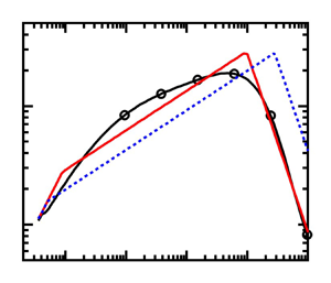
Figure 1 shows the profiles of the scalar fluxes as functions of  $y$ for the two cases. Here, ‘DNS’ denotes $\langle u_y \theta \rangle$ evaluated directly, ‘Local’ denotes $\langle u_y \theta \rangle _{L}$ given by (2.10) and ‘Non-local’ denotes $\langle u_y \theta \rangle _{NL}$ given by (2.8). The profiles of $\langle u_y \theta \rangle _{NL}$ plotted as blue dotted lines agree with the DNS values for both cases. This agreement verifies the non-local expression for the scalar flux given by (2.8). In contrast, the profiles of $\langle u_y \theta \rangle _{L}$, plotted as red lines, overpredicted the DNS values. The small value of the DNS compared with the local model can be accounted for by the non-local effect (Hamba Reference Hamba2022b). The overprediction by the local model was more significant in case 2 than in case 1 because the length scale of the mean scalar field was small in case 2.

Figure 1. Profiles of the scalar fluxes  $\langle u_y \theta \rangle$, $\langle u_y \theta \rangle _{L}$ and $\langle u_y \theta \rangle _{NL}$ as functions of $y$ for (a) case 1 and (b) case 2.
Figure 2 shows the profiles of the non-local eddy diffusivity  $\kappa _{NLyy}(\kern0.03em y-y^\prime )$ as functions of $(\kern0.03em y-y^\prime )/L$. The separation $y-y^\prime$ was normalised by the integral length scale $L$, whose value is 0.465 in the present DNS (see also Appendix B). The non-local eddy diffusivity $\kappa _{NLyy}(\kern0.03em y-y^\prime )$ is of the same dimension as the velocity and is non-dimensionalised by $\langle u_i^2\rangle ^{1/2}$. The black line represents the DNS value obtained from (2.9), which was used to evaluate $\langle u_y\theta \rangle _{NL}$ plotted in figure 1, whereas the other lines for models 1 and 2 are mentioned later. As the profile is symmetric with respect to $(\kern0.03em y-y^\prime )/L=0$, it is plotted only in the positive region at $(\kern0.03em y-y^\prime )/L\geq 0$. It exhibits a sharp peak at $(\kern0.03em y-y^\prime )/L=0$ and decays quickly as $(\kern0.03em y-y^\prime )/L$ increases. The profile suggests that the value of $\partial \varTheta /\partial y^\prime$ within the integral length scale at $-L< y-y^\prime < L$ mainly affects the scalar flux at $y$ in (2.8).

Figure 2. Profiles of the non-local eddy diffusivity  $\kappa _{NLyy}(\kern0.03em y-y^\prime )$ as functions of $(\kern0.03em y-y^\prime )/L$ for DNS and models 1 and 2.
We demonstrated the non-local eddy diffusivity  $\kappa _{NLyy}(\kern0.03em y-y^\prime )$ in the case of one-dimensional profiles of the mean scalar $\varTheta (\kern0.03em y)$. However, in the case of general profiles of the mean scalar varying in three directions, we must consider the original expression for the three-dimensional non-local eddy diffusivity
 \begin{equation} \kappa_{NLij}(\boldsymbol{r},\tau)= \langle u_i(\boldsymbol{x},t)g_j(\boldsymbol{x},t;\boldsymbol{x}^\prime,t^\prime)\rangle , \end{equation}
which is a function of  $\boldsymbol {r}(=\boldsymbol {x}-\boldsymbol {x}^\prime )$ and $\tau (=t-t^\prime )$ for homogeneous and steady turbulence. Because the turbulent velocity field is isotropic and the Green's function is determined solely by the velocity fluctuation, the non-local eddy diffusivity can be expressed in the isotropic form
 \begin{equation} \kappa_{NLij}(\boldsymbol{r},\tau)=\kappa_{NL}(r,\tau)\delta_{ij} , \end{equation}
where  $\kappa _{NL}(r,\tau )=\kappa _{NLii}(\boldsymbol {r},\tau )/3$ and $r=|\boldsymbol {r}|$, and a term proportional to $r_ir_j/r^2$ was neglected. Next, we investigated the three-dimensional non-local eddy diffusivity $\kappa _{NL}(r,\tau )$ and its time integral $\kappa _{NL}(r)$, which is given by
 \begin{equation} \kappa_{NL}(r)=\int_{0}^{\infty}\,\mathrm{d}\tau\kappa_{NL}(r,\tau) . \end{equation}
The one-dimensional non-local eddy diffusivity  $\kappa _{NLyy}(\kern0.03em y-y^\prime )$ can be obtained from
 \begin{equation} \kappa_{NLyy}(r_y)=\int_{-\infty}^{\infty}\,{\mathrm{d}r_x}\int_{-\infty}^{\infty}\,{\mathrm{d}r_z}\kappa_{NL}(r)=\int_{r_y}^{\infty}\,\mathrm{d}r2{\rm \pi} r\kappa_{NL}(r) . \end{equation}
 In Hamba (Reference Hamba2022b) we modelled the three-dimensional non-local eddy diffusivity  $\kappa _{NL}(r,\tau )$ using the two-point velocity correlation $Q_{ii}(\boldsymbol {r})(=\langle u_i(\boldsymbol {x},t)u_i(\boldsymbol {x}^\prime,t)\rangle )$ as
 \begin{equation} \kappa_{NL}(r,\tau)=G(r,\tau)Q(r), \end{equation}
where  $Q(r)=Q_{ii}(\boldsymbol {r})/3$. The statistical theory of turbulence suggested that the two-time velocity correlation $Q_{ii}(\boldsymbol {r},\tau )(=\langle u_i(\boldsymbol {x},t)u_i(\boldsymbol {x}^\prime,t^\prime )\rangle )$ must be used instead of the one-time correlation $Q_{ii}(\boldsymbol {r})$ (Kraichnan Reference Kraichnan1964; Yoshizawa Reference Yoshizawa1998). Nevertheless, considering its application to inhomogeneous turbulence in the near future, we adopted the one-time correlation $Q_{ii}(\boldsymbol {r})$ in (2.16) because it is simple (see also Appendix C). The time-dependent part $G(r,\tau )$ appearing in (2.16), which corresponds to the mean Green's function for the scalar fluctuation, was given by
 \begin{equation} G(r,\tau)=\frac{1}{(4{\rm \pi})^{3/2}(C_{\omega G}u_0\tau)^3}\exp\left[-\frac{r^2}{4(C_{\omega G}u_0\tau)^2}\right] , \end{equation}
where  $u_0=\langle u_i^2\rangle ^{1/2}=(2K)^{1/2}$, $K(=\langle u_i^2\rangle /2)$ is the turbulent kinetic energy and $C_{\omega G}$ is a model constant. The function given by (2.17) was determined by referring to the temporal behaviour of the two-time velocity correlation $Q(r,\tau )$ evaluated using DNS (Hamba Reference Hamba2022b). For the velocity correlation $Q(r)$, we used the Fourier transform and assumed the Kolmogorov energy spectrum in the inertial range as
 \begin{gather} Q_{ii}(\boldsymbol{r})=\int\, \mathrm{d}\boldsymbol{k}Q_{ii}(\boldsymbol{k})\exp{(\mathrm{i}\boldsymbol{k}\boldsymbol{\cdot}\boldsymbol{r})}=\int_{0}^{\infty}\,\mathrm{d}k2E(k)\frac{\sin{(kr)}}{kr} , \end{gather}
 \begin{gather} E(k)=\left\{\begin{matrix}C_K\varepsilon^{2/3}k^{{-}5/3}, & k_c\le k\le k_d\\ 0, & k< k_c,\quad k>k_d \end{matrix}\right. , \end{gather}
where  $k=|\boldsymbol {k}|$, $E(k)(=2{\rm \pi} k^2Q_{ii}(\boldsymbol {k}))$ is the energy spectrum, $C_K$ is a model constant and $\varepsilon [=\nu \langle (\partial u_i/\partial x_j)^2\rangle ]$ is the energy dissipation rate. The quantity $Q_{ii}(\boldsymbol {k})$ has a relationship $Q_{ii}(\boldsymbol {k})\delta (\boldsymbol {k}+\boldsymbol {k}')=\langle \tilde {u}_{i}(\boldsymbol {k})\tilde {u}_{i}(\boldsymbol {k}')\rangle$, where $\tilde {u}_{i}(\boldsymbol {k})$ is the Fourier transform of the velocity fluctuation. In (2.19) two cutoff wavenumbers were introduced, $k_c\{=[(3C_K/2)^{-1}K\varepsilon ^{-2/3}+k_d^{-2/3}]^{-3/2}\}$ in the energy-containing range and $k_d[=(3C_K/2)^{-3/4}\nu ^{-3/4}\varepsilon ^{1/4}]$ in the dissipation range. The cutoff at $k=k_{c}$ does not mean that the energy in the energy-containing range is completely ignored but that the form of the energy spectrum is approximated using a step function. In the statistical theory of turbulence, Yoshizawa (Reference Yoshizawa1984) also used the same energy spectrum to appropriately evaluate the eddy viscosity. To improve the model, other forms can be used such as the von Kármán spectrum $E(k) \propto (k/k_{c})^{4}/[1+(k/k_{c})^{2}]^{17/6}$(Hinze Reference Hinze1975). In Hamba (Reference Hamba2022b), (2.19) was adopted as the first approximation. Finally, we obtained a model expression for $\kappa _{NL}(r,\tau )$ given by (2.16) with (2.17)–(2.19).
Two model constants  $C_{K}$ and $C_{\omega G}$ were used in the above model; their values are listed as model 1 in table 1. The value of $C_K=1.1$ is fairly small compared with a well-known value of $C_K=1.7$ for the Kolmogorov constant (Kaneda Reference Kaneda1986). A small value of $C_{K}$ leads to a small value of $k_{c}$ appearing in (2.19), corresponding to a large value of the integral length scale. As a result, the profile of $Q_{ii}(\boldsymbol {r})$ for model 1 is wider than the DNS value. However, such a wide profile was necessary to accurately predict the non-local eddy diffusivity $\kappa _{NL}(r,\tau )$ using (2.16) (Hamba Reference Hamba2022b). The profile of $\kappa _{NLyy}(\kern0.03em y-y^\prime )$ obtained from (2.15) and (2.16) with $C_K=1.1$ was plotted as a red line in figure 2. It agrees with the DNS value plotted as a black line. Using this model, we predicted the turbulent scalar flux that agrees with the DNS data (not shown here). In the present model, the energy spectrum $E(k)$ was used to express the velocity correlation appearing in (2.16). Because the Fourier transform of velocity in the homogeneous directions was used to define the energy spectrum, it is not clear whether the present model can be applied to inhomogeneous turbulence.
Table 1. Equations for model expression and the values of model constants for the non-local eddy diffusivity  $\kappa _{NL}(r,\tau )$ given by (2.16).

3. Non-local eddy diffusivity based on scale-space energy density
In the non-local eddy diffusivity model described in § 2, the energy spectrum was used to express the two-point velocity correlation in (2.16). In applying the model to inhomogeneous turbulence, the two-point correlation must be expressed in terms of quantities in physical space representing the scale-space energy instead of the energy spectrum. A candidate is the scale-space energy density based on filtered velocities (Hamba Reference Hamba2022a). The turbulent energy was decomposed into the scale-space energy density even in the wall-normal direction of a channel flow. In this study we apply this formulation to the two-point correlation required for the non-local eddy diffusivity in preparation for developing a non-local model for inhomogeneous turbulence.
3.1. Formulation of scale-space quantities using filtered velocities
We introduce two filtered velocities using different filter functions (Hamba Reference Hamba2022a). The first filtered velocity  ${\bar {u}}_i(\boldsymbol {x},s)$ is an ordinary one with a Gaussian filter that is widely used in LES. It is defined as
 \begin{equation} {\bar{u}}_i(\boldsymbol{x},s)=\int\,{\mathrm{d}\kern0.06em \boldsymbol{x}^\prime}\bar{G}(\boldsymbol{x}-\boldsymbol{x}^\prime,s)u_i(\boldsymbol{x}^\prime) , \end{equation}
where  $\bar {G}(\boldsymbol {x},s)$ is the filter function given by
 \begin{equation} \bar{G}(\boldsymbol{x},s)=\frac{1}{{(2{\rm \pi} s)}^{3/2}}\exp\left(-\frac{\boldsymbol{x}^2}{2s}\right) . \end{equation}
Note that instead of the filter width  $\varDelta$, we adopt a quantity $s$ with a dimension of the square of the length in (3.1) and (3.2); hereafter, we refer $s$ as the scale. The filtered velocity ${\bar {u}}_i(\boldsymbol {x},s)$ represents the velocity with a scale equal to or greater than $s$. The velocity also depends on time $t$, but it is omitted for simplicity in § 3.
By differentiating  ${\bar {u}}_i(\boldsymbol {x},s)$ with respect to $s$, we can obtain a filtered velocity with a scale equal to $s$. We define the second filtered velocity ${\hat {u}}_i(\boldsymbol {x},s)$ as
 \begin{equation} {\hat{u}}_i(\boldsymbol{x},s)\equiv{-}\frac{\partial}{\partial s}{\bar{u}}_i(\boldsymbol{x},s)=\int\,{\mathrm{d}\kern0.06em \boldsymbol{x}^\prime}\hat{G}(\boldsymbol{x}-\boldsymbol{x}^\prime,s)u_i(\boldsymbol{x}^\prime) , \end{equation}
where
 \begin{equation} \hat{G}(\boldsymbol{x},s)\equiv{-}\frac{\partial}{\partial s}\bar{G}(\boldsymbol{x},s)=\frac{1}{{(2{\rm \pi} s)}^{3/2}}\left(\frac{3}{2s}-\frac{\boldsymbol{x}^2}{2s^2}\right)\exp\left(-\frac{\boldsymbol{x}^2}{2s}\right) . \end{equation}
The original velocity  $u_i(\boldsymbol {x})$ can be written in terms of ${\hat {u}}_i(\boldsymbol {x},s)$ as
 \begin{equation} u_i(\boldsymbol{x})=\int_{0}^{\infty}\,\mathrm{d}s{\hat{u}}_i(\boldsymbol{x},s) . \end{equation}
This equation indicates that the velocity  $u_i(\boldsymbol {x})$ is decomposed into the modes ${\hat {u}}_i(\boldsymbol {x},s)$ in the scale space.
Following that, we consider the two-point correlation of filtered velocities at the same scale defined as
 \begin{equation} {\bar{Q}}_{ii}(\boldsymbol{x}_1,\boldsymbol{x}_2,s)=\langle {\bar{u}}_i(\boldsymbol{x}_1,s){\bar{u}}_i(\boldsymbol{x}_2,s)\rangle . \end{equation}
Another correlation can be defined as
 \begin{equation} {\hat{Q}}_{ii}(\boldsymbol{x}_1,\boldsymbol{x}_2,s)\equiv{-}\frac{\partial}{\partial s}{\bar{Q}}_{ii}(\boldsymbol{x}_1,\boldsymbol{x}_2,s)= \langle {\hat{u}}_i(\boldsymbol{x}_1,s){\bar{u}}_i(\boldsymbol{x}_2,s)\rangle + \langle {\bar{u}}_i(\boldsymbol{x}_1,s){\hat{u}}_i(\boldsymbol{x}_2,s)\rangle . \end{equation}
Using the second correlation  ${\hat {Q}}_{ii}(\boldsymbol {x}_1,\boldsymbol {x}_2,s)$, we can decompose the original velocity correlation $Q_{ii}(\boldsymbol {x}_1,\boldsymbol {x}_2)(=\langle u_i(\boldsymbol {x}_1)u_i(\boldsymbol {x}_2)\rangle )$ into modes in the scale space as follows:
 \begin{equation} Q_{ii}(\boldsymbol{x}_1,\boldsymbol{x}_2)=\int_{0}^{\infty}\,\mathrm{d}s{\hat{Q}}_{ii}(\boldsymbol{x}_1,\boldsymbol{x}_2,s) . \end{equation}
In the case of homogeneous turbulence, (3.8) can be rewritten as
 \begin{equation} Q_{ii}(\boldsymbol{r})=\int_{0}^{\infty}\,\mathrm{d}s{\hat{Q}}_{ii}(\boldsymbol{r},s) , \end{equation}
where  $\boldsymbol {r}=\boldsymbol {x}_1-\boldsymbol {x}_2$. Therefore, when we know the value of the scale-space correlation ${\hat {Q}}_{ii}(\boldsymbol {r},s)$, we can evaluate the original correlation $Q_{ii}(\boldsymbol {r})$ using (3.9) in place of (2.18) in which the energy spectrum was used.
Applying the filter function to the original velocity correlation, we can express the first and second correlations as
 \begin{gather} {\bar{Q}}_{ii}(\boldsymbol{r},s)=\int\,{\mathrm{d}\boldsymbol{r}^\prime}\bar{G}(\boldsymbol{r}-\boldsymbol{r}^\prime,2s)Q_{ii}(\boldsymbol{r}^\prime) , \end{gather}
 \begin{gather} {\hat{Q}}_{ii}(\boldsymbol{r},s)=\int\,{\mathrm{d}\boldsymbol{r}^\prime}2\hat{G}(\boldsymbol{r}-\boldsymbol{r}^\prime,2s)Q_{ii}(\boldsymbol{r}^\prime) . \end{gather}
These equations indicate that the correlation of filtered velocities can be obtained by filtering the original velocity correlation. Equation (3.10) is similar to the relation between the subgrid stress and the second-order structure function derived by Germano (Reference Germano2007). Using the energy spectrum, the second correlation  ${\hat {Q}}_{ii}(\boldsymbol {r},s)$ is also written as
 \begin{equation} {\hat{Q}}_{ii}(\boldsymbol{r},s)=\int \,\mathrm{d}\boldsymbol{k}Q_{ii}(\boldsymbol{k})k^2\exp({-}sk^2)\exp(\mathrm{i}\boldsymbol{k}\boldsymbol{\cdot}\boldsymbol{r})=\int_{0}^{\infty}\,\mathrm{d}k2E(k)k^2\exp({-}sk^2)\frac{\sin(kr)}{kr} . \end{equation}
Comparing (3.12) with (2.18),  ${\hat {Q}}_{ii}(\boldsymbol {r},s)$ corresponds to a band-pass filtered spectrum $E(k)k^2\exp (-sk^2)$ in the wavenumber space.
3.2. Energy density in scale space
To examine the behaviour of the scale-space correlation  ${\hat {Q}}_{ii}(\boldsymbol {r},s)$ and its relation to the two-point correlation $Q_{ii}(\boldsymbol {r})$, we first treat the case of $\boldsymbol {r}=\boldsymbol {0}$. The one-point velocity correlation represents the turbulent kinetic energy, $Q_{ii}(\boldsymbol {0})=\langle u_i^2\rangle$, and (3.9) is rewritten as
 \begin{equation} \langle u_i^2\rangle =\int_{0}^{\infty}\,\mathrm{d}s{\hat{Q}}_{ii}(s) , \end{equation}
where  ${\hat {Q}}_{ii}(s)(={\hat {Q}}_{ii}(\boldsymbol {0},s))$ is the energy density in the scale space. Particularly, $\langle u_i^2\rangle$ is twice the turbulent energy, but we call it the turbulent energy for simplicity. Equation (3.13) indicates that the turbulent energy is decomposed into the scale-space energy density ${\hat {Q}}_{ii}(s)$. Figure 3 shows profiles of the pre-multiplied energy density ${s\hat {Q}}_{ii}(s)$ as functions of $s$. The black line represents the energy density obtained from the DNS of homogeneous isotropic turbulence described in § 2.


Figure 4. Profiles of two-point correlations at six scales in the scale space: (a)  ${\hat {Q}}_{ii}(\boldsymbol {r},s)$ as functions of $r/L$ and (b) ${\hat {Q}}_{ii}(\boldsymbol {r},s)/{\hat {Q}}_{jj}(s)$ as functions of $r/s^{1/2}$. The red line denotes the function $\exp (-r^2/4s)$.
The profile of the energy density  ${\hat {Q}}_{ii}(s)$ can be understood as follows. In the case of $r=0$, (3.12) is rewritten as
 \begin{equation} {\hat{Q}}_{ii}(s)=\int_{0}^{\infty}\,\mathrm{d}k2E(k)k^2\exp({-}sk^2) . \end{equation}
By substituting the Kolmogorov energy spectrum  ${E(K)=C}_K\varepsilon ^{2/3}k^{-5/3}$ into (3.14), we can obtain the inertial-range form of ${\hat {Q}}_{ii}(s)$ as
 \begin{equation} {\hat{Q}}_{ii}(s)=\int_{0}^{\infty}\,\mathrm{d}k2C_K\varepsilon^{2/3}k^{{-}5/3}k^2\exp{({-}sk^2)}=\varGamma\big({\tfrac{2}{3}}\big)C_K\varepsilon^{2/3}s^{{-}2/3} , \end{equation}
where  $\varGamma (x)$ is the gamma function and $\varGamma (2/3)=1.354$. Therefore, the energy density ${\hat {Q}}_{ii}(s)$ is expected to be proportional to $s^{-2/3}$ in the inertial range. The pre-multiplied energy density is then proportional to $s^{1/3}$.
As the scale  $s$ decreases to zero in the dissipation range, the energy density ${\hat {Q}}_{ii}(s)$ tends to a constant value rather than increasing infinitely. By substituting $s=0$ into (3.14), we obtain
 \begin{equation} {\hat{Q}}_{ii}(0)=\int_{0}^{\infty}\,\mathrm{d}k2k^2E(k)=\nu^{{-}1}\varepsilon . \end{equation}
The energy density  ${\hat {Q}}_{ii}(0)$ is closely related to the energy dissipation $\varepsilon$. Conversely, at the scale $s$ much greater than the square of the integral length scale, the energy density ${\hat {Q}}_{ii}(s)$ shows a different behaviour than that in the inertial range. In the case of $r=0$, (3.11) is rewritten as
 \begin{equation} {\hat{Q}}_{ii}(s)=\int \,\mathrm{d}\boldsymbol{r}2\hat{G}(\boldsymbol{r},2s)Q_{ii}(\boldsymbol{r}) . \end{equation}
Approximately, the original velocity correlation  $Q_{ii}(\boldsymbol {r})$ has non-zero values at $|\boldsymbol {r}|< L$ and tends to zero at $|\boldsymbol {r}|\gg L$, where $L$ is the integral length scale. If $s\gg L^2$ and $s\gg \boldsymbol {r}^2$, the filter function defined as (3.4) can be approximated as
 \begin{equation} \hat{G}(\boldsymbol{r},s)\cong\frac{1}{{(2{\rm \pi} s)}^{3/2}}\frac{3}{2s} , \end{equation}
in the region of the non-zero value of  $Q_{ii}(\boldsymbol {r})$ in (3.17). Because (3.18) does not depend on $\boldsymbol {r}$, we have
 \begin{equation} {\hat{Q}}_{ii}(s)=2\frac{1}{{(4{\rm \pi} s)}^{3/2}}\frac{3}{4s}\int \,\mathrm{d}\boldsymbol{r}Q_{ii}(\boldsymbol{r})\propto s^{{-}5/2} . \end{equation}
The energy density  ${\hat {Q}}_{ii}(s)$ is proportional to $s^{-5/2}$ at the scale $s$ much greater than $L^{2}$.
Considering the above behaviour of  ${\hat {Q}}_{ii}(s)$, we can assume a simple form of ${\hat {Q}}_{ii}(s)$ as
 \begin{equation} {\hat{Q}}_{ii}(s)=
\left\{\begin{matrix}\nu^{{-}1}\varepsilon, & s<
s_d, \\ C_s\varepsilon^{2/3}s^{{-}2/3}, & s_d\le
s\le s_c, \\
C_s\varepsilon^{2/3}s_c^{11/6}s^{{-}5/2}, & s>s_c,
\\ \end{matrix}\right. \end{equation}
\begin{equation} {\hat{Q}}_{ii}(s)=
\left\{\begin{matrix}\nu^{{-}1}\varepsilon, & s<
s_d, \\ C_s\varepsilon^{2/3}s^{{-}2/3}, & s_d\le
s\le s_c, \\
C_s\varepsilon^{2/3}s_c^{11/6}s^{{-}5/2}, & s>s_c,
\\ \end{matrix}\right. \end{equation}
where  $C_s$ is a model constant and two interface scales are introduced, $s_d(={C_s}^{3/2}\nu ^{3/2}\varepsilon ^{-1/2})$ in the dissipation range and $s_c[=(6/11)^3{C_s}^{-3}K^3\varepsilon ^{-2}(1+{C_s}^{3/2}\nu ^{1/2}K^{-1} \varepsilon ^{1/2})^3]$ in the energy-containing range. The scale $s_d$ is obtained by connecting the forms in the two ranges $s< s_d$ and $s_d\le s\le s_c$, whereas the scale $s_c$ is determined so that (3.13) can be satisfied. The model constant $C_s$ can be estimated when not only the turbulent energy $K$ but also the integral length scale $L$ are known. It is given by
 \begin{equation} C_s=\big(\tfrac{9}{10}\big)^{2/3}\tfrac{6}{11}{\rm \pi}^{1/3}K\varepsilon^{{-}2/3}L^{{-}2/3} , \end{equation}
(see Appendix B for details). In the present DNS where  $K=0.50$, $\varepsilon =0.19$ and $L=0.47$, it is estimated as $C_s=1.9$. The profile of the pre-multiplied energy density $s{\hat {Q}}_{ii}(s)$ given by (3.20) with $C_s=1.9$ is plotted as a red line in figure 3. It reasonably agrees with the DNS value plotted as a black line. Therefore, (3.20) can be a simple form of the scale-space energy density corresponding to the Kolmogorov energy spectrum given by (2.19).
3.3. Two-point velocity correlation in scale space
The energy spectrum  $E(k)$ and the two-point correlation $Q_{ii}(\boldsymbol {r})$ have equivalent information; we can evaluate $Q_{ii}(\boldsymbol {r})$ using (2.18) when we know the value of $E(k)$. The simple form of $E(k)$ given by (2.19) constitutes a model for $Q_{ii}(\boldsymbol {r})$. In contrast, we cannot evaluate $Q_{ii}(\boldsymbol {r})$ even when we know the value of the energy density ${\hat {Q}}_{ii}(s)$. Rather than ${\hat {Q}}_{ii}(s)$, the scale-space correlation ${\hat {Q}}_{ii}(\boldsymbol {r},s)$ is necessary to determine $Q_{ii}(\boldsymbol {r})$ using (3.9). In § 3.3 we try to relate ${\hat {Q}}_{ii}(\boldsymbol {r},s)$ to ${\hat {Q}}_{ii}(s)$ to determine $Q_{ii}(\boldsymbol {r})$ by ${\hat {Q}}_{ii}(s)$.
We obtain the relationship between  ${\hat {Q}}_{ii}(\boldsymbol {r},s)$ and ${\hat {Q}}_{ii}(s)$ with the help of $E(k)$. The scale-space correlation ${\hat {Q}}_{ii}(\boldsymbol {r},s)$ is related to $E(k)$ as shown in (3.12). The function $k^2\exp (-sk^2)$ appearing in (3.12) plays a role of a band-pass filter in the wavenumber space and it shows a maximum value at $k=s^{-1/2}$. Assuming the energy spectrum $E(k)$ changes slowly in the wavenumber region of the band-pass filter, we consider the Taylor expansion of $E(k)$ around $k=s^{-1/2}$ as follows:
 \begin{equation} E(k)=E(s^{{-}1/2})+\left.\frac{{\rm d}E}{{\rm d}k}\right|_{k=s^{{-}1/2}}(k-s^{{-}1/2})+\frac{1}{2}\left.\frac{{\rm d}^2E}{{\rm d}k^2}\right|_{k=s^{{-}1/2}}{(k-s^{{-}1/2})}^2+\cdots . \end{equation}
Substituting the first term in (3.22) into (3.12), we obtain
 \begin{equation} {\hat{Q}}_{ii}(\boldsymbol{r},s)=\int_{0}^{\infty}\,\mathrm{d}k2E(s^{{-}1/2})k^2\exp({-}sk^2)\frac{\sin(kr)}{kr}=\frac{{\rm \pi}^{1/2}}{2s^{3/2}}E(s^{{-}1/2})\exp\left(-\frac{r^2}{4s}\right) . \end{equation}
This expression suggests that the scale-space correlation  ${\hat {Q}}_{ii}(\boldsymbol {r},s)$ is proportional to $\exp (-r^2/4s)$. The profile of ${\hat {Q}}_{ii}(\boldsymbol {r},s)$ at scale $s$ shows a length scale of $s^{1/2}$. Considering the condition ${\hat {Q}}_{ii}(\boldsymbol {0},s)={\hat {Q}}_{ii}(s)$, we then propose an approximate relationship between ${\hat {Q}}_{ii}(\boldsymbol {r},s)$ and ${\hat {Q}}_{ii}(s)$ as follows:
 \begin{equation} {\hat{Q}}_{ii}(\boldsymbol{r},s)={\hat{Q}}_{ii}(s)\exp\left(-\frac{r^2}{4s}\right) . \end{equation}
Substituting (3.24) into (3.9), we obtain
 \begin{equation} Q_{ii}(\boldsymbol{r})=\int_{0}^{\infty}\,\mathrm{d}s{\hat{Q}}_{ii}(s)\exp\left(-\frac{r^2}{4s}\right) . \end{equation}
Therefore, using (3.25) we can determine  $Q_{ii}(\boldsymbol {r})$ when we know the value of ${\hat {Q}}_{ii}(s)$, although (3.25) is an approximate expression. Note that the value of $E(k)$ is not necessary once we obtain the relationship (3.25).
Figure 4(a) shows the profiles of  ${\hat {Q}}_{ii}(\boldsymbol {r},s)$ as functions of $r/L$ at six scales varying from $s=0.00094$ to 0.96. The locations of the six scales are plotted as symbols in figure 3. In figure 4(a) each profile shows a peak value at $r/L=0$ and decays to zero as $r/L$ increases. As $s$ increases, the peak value decreases and the profile becomes wider. The proposed relationship given by (3.24) suggests that the separation $r$ can be scaled by $s^{1/2}$. Figure 4(b) shows the profiles of ${\hat {Q}}_{ii}(\boldsymbol {r},s)$ normalised by ${\hat {Q}}_{ii}(s)$ as functions of $r/s^{1/2}$ at six scales. If the relationship given by (3.24) holds exactly, the profiles must be self-similar and agree with the function $\exp (-r^2/4s)$, which is plotted as a red line in figure 4(b). Despite the self-similarity not holding very well, the function approximately reproduces overall profiles decaying as $r/s^{1/2}$ increases. In the case of $s=0.060$, the profile of ${\hat {Q}}_{ii}(\boldsymbol {r},s)/{\hat {Q}}_{jj}(s)$ agrees well with the function. Because the scale of $s=0.060$ corresponds to the energy-containing range as shown in figure 3 and $E(k)$ is expected not to change very much, the first term in (3.22) can be a good approximation in the integral in (3.12). The deviation of the other profiles from the function can be understood by considering the effect of the second term in (3.22) on the integral in (3.12). In the case of three scales less than $s=0.060$, ${\hat {Q}}_{ii}(\boldsymbol {r},s)/{\hat {Q}}_{jj}(s)$ shows a wide profile compared with $\exp (-r^2/4s)$. At corresponding higher wavenumbers in the inertial range, ${\rm d}E/{\rm d}k$ is negative; owing to the second term in (3.22) the lower wavenumber part of $E(k)$ at $k< s^{-1/2}$ contributes to the integral more than the higher wavenumber part does, which accounts for the wide profiles of ${\hat {Q}}_{ii}(\boldsymbol {r},s)/{\hat {Q}}_{jj}(s)$. In contrast, in the case of two scales greater than $s=0.060$, ${\hat {Q}}_{ii}(\boldsymbol {r},s)/{\hat {Q}}_{jj}(s)$ shows a narrow profile compared with $\exp (-r^2/4s)$. At corresponding very low wavenumbers, ${\rm d}E/{\rm d}k$ is positive; the higher wavenumber part of $E(k)$ at $k>s^{-1/2}$ contributes to the integral more, which accounts for the narrow profiles of ${\hat {Q}}_{ii}(\boldsymbol {r},s)/{\hat {Q}}_{jj}(s)$.
Figure 5 shows the profiles of the two-point velocity correlation  $Q_{ii}(\boldsymbol {r})$ as functions of $r/L$. The black line represents the correlation obtained from the DNS. The profile evaluated from (3.25) and (3.20) with $C_s=1.9$ is plotted as a red line; it agrees fairly well with the DNS value. Because the energy density ${\hat {Q}}_{ii}(s)$ and the function $\exp (-r^2/4s)$ are both positive, the model given by (3.25) gives a positive value; it cannot reproduce a small negative value of $Q_{ii}(\boldsymbol {r})$ around $r/L=3$. To express $Q_{ii}(\boldsymbol {r})$ more accurately, we must incorporate the second term in (3.22) into (3.12). However, our objective is not very accurate modelling of $Q_{ii}(\boldsymbol {r})$ but modelling of the non-local eddy diffusivity that was suggested to be non-negative in our previous analysis. We then adopt an approximate relationship given by (3.25) in the present study.


3.4. Modelling the non-local eddy diffusivity
In § 3.3 the velocity correlation  $Q_{ii}(\boldsymbol {r})$ was expressed in terms of the energy density ${\hat {Q}}_{ii}(s)$ in (3.25), and a simple form of ${\hat {Q}}_{ii}(s)$ was proposed as (3.20). Therefore, we obtained another model expression for $\kappa _{NL}(r,\tau )$ given by (2.16) with (2.17), (3.20) and (3.25), for which the scale-space energy density was used instead of the energy spectrum. Despite (3.20) with $C_s=1.9$ giving a good profile of $Q_{ii}(\boldsymbol {r})$ in figure 5, it leads to a narrow profile of $\kappa _{NLyy}(\kern0.03em y-y^\prime )$ compared with the DNS value (not shown here). This situation is similar to the previous model with the energy spectrum; the profile of $\kappa _{NLyy}(\kern0.03em y-y^\prime )$ obtained from the model with $C_K=1.7$ is too narrow and we needed to change the value to $C_K=1.1$ to obtain a good profile (Hamba Reference Hamba2022b). Therefore, in this study, we also optimised the model constants to ensure that the profile of $\kappa _{NLyy}(\kern0.03em y-y^\prime )$ agrees with the DNS value. The optimised values are $C_s=1.3$ and $C_{\omega G}=0.46$, which are listed as model 2 in table 1. The profiles of ${\hat {Q}}_{ii}(s)$ and $Q_{ii}(\boldsymbol {r})$ for $C_s=1.3$ are shown as blue dotted lines in figures 3 and 5, respectively. As $C_s$ decreases from 1.9 to 1.3, the scale $s_c$ in the energy-containing range appearing in (3.20), which corresponds to the peak location of $s{\hat {Q}}_{ii}(s)$, increases as shown in figure 3. The profile of $Q_{ii}(\boldsymbol {r})$ then becomes wider as shown in figure 5. Therefore, the profile of $\kappa _{NLyy}(\kern0.03em y-y^\prime )$ obtained from model 2 plotted as a blue dotted line agrees with the DNS value in figure 2.
The previous and new models listed in table 1 gave good profiles of the one-dimensional non-local eddy diffusivity  $\kappa _{NLyy}(\kern0.03em y-y^\prime )$ in figure 2. Furthermore, we also examine the three-dimensional non-local eddy diffusivity $\kappa _{NL}(r)$ and $\kappa _{NL}(r,\tau )$. Figure 6 shows the profiles of $r^2\kappa _{NL}(r)$ as functions of $r/L$. As $r/L$ increases, the profiles of models 1 and 2 decay a little slowly compared with the DNS value, and the profile of model 2 is better than that of model 1. By substituting (2.17) into (2.16) and calculating the integral in (2.14), we obtain
 \begin{equation} \kappa_{NL}(r)=\frac{1}{12{\rm \pi}^{3/2}C_{\omega G}u_0r^2}Q_{ii}(\boldsymbol{r}) . \end{equation}
Therefore, the difference in  $r^2\kappa _{NL}(r)$ between the two models is attributed to the difference in $C_{\omega G}$ and $Q_{ii}(\boldsymbol {r})$; its peak value at $r/L=0$ is inversely proportional to $C_{\omega G}$ and the width of the profile depends on $Q_{ii}(\boldsymbol {r})$.

Figure 6. Profiles of  $r^2\kappa _{NL}(r)$ as functions of $r/L$ for DNS and models 1 and 2.
The difference between the two models is clearly seen in the profile of  $\kappa _{NL}(r,\tau )$. Figure 7 shows the profiles of $\kappa _{NL}(r,\tau )$ as functions of $r/L$ at $\tau =0.2$, 0.4, 0.6 and 0.8. The four time differences are short compared with the turbulent time scale $T(=K/\varepsilon )=2.7$ in the present DNS. The black lines represent the DNS values; the profile of $\kappa _{NLii}(r_y,\tau )$ was first obtained by averaging over the $x$–
$x$– $z$ plane and 120 samples, and the profile of $\kappa _{NL}(r,\tau )$ was evaluated using the same relationship as (2.15). As the time difference $\tau$ increased, the peak value at $r/L=0$ decayed rapidly and the width increased gradually. This behaviour implies that the spatial region in which the mean scalar gradient non-locally affects the scalar flux is highly narrow for small $\tau$ and becomes wider as $\tau$ increases (Hamba Reference Hamba2022b). The profiles of model 1 plotted as red lines show small values, whereas those of model 2 plotted as blue dotted lines agree well with the DNS values. Therefore, model 2 is more appropriate than model 1 for reproducing the temporal behaviour of $\kappa _{NL}(r,\tau )$. This difference between the two models could be attributed to the difference in the basis function in the expression for $Q_{ii}(\boldsymbol {r})$. For model 1, the correlation $Q_{ii}(\boldsymbol {r})$ is decomposed into modes with $\sin (kr)/kr$ in (2.18) whereas, for model 2, it is decomposed into modes with $\exp (-r^2/4s)$ in (3.25). The basis function $\exp (-r^2/4s)$ is similar to the filter function $\bar {G}(\boldsymbol {x},s)$ given by (3.2), which can be interpreted as a solution of the diffusion equation if the scale $s$ is considered as time. Because the temporal behaviour of $\kappa _{NL}(r,\tau )$ is closely related to the turbulent diffusion process, model 2 with the basis function $\exp (-r^2/4s)$ can be more appropriate for reproducing such a diffusion process (see also Appendix C).

Figure 7. Profiles of  $\kappa _{NL}(r,\tau )$ as functions of $r/L$ for DNS and models 1 and 2 at (a) $\tau =0.2$, (b) $\tau =0.4$, (c) $\tau =0.6$ and (d) $\tau =0.8$.
Moreover, the new model has an advantage over the previous model in its applicability to inhomogeneous turbulence. The Fourier transform of velocity in the homogeneous directions was used to define the energy spectrum  $E(k)$; it is not clear whether the previous model with the energy spectrum can be applied to inhomogeneous turbulence. In contrast, the scale-space energy density ${\hat {Q}}_{ii}(s)$ was already examined in a turbulent channel flow, and the turbulent energy was adequately decomposed in the scale space even in the inhomogeneous wall-normal direction (Hamba Reference Hamba2022a). This was performed by extending the filter function $\bar {G}(\boldsymbol {x},s)$ to the solution of the diffusion equation. The filter function given by (3.2) is the solution of the following equation in infinite domain:
 \begin{equation} \frac{\partial}{\partial s} \bar{G}(\boldsymbol{x},s) = \frac{1}{2} \frac{\partial^{2}}{\partial x^{2}_{i}} \bar{G}(\boldsymbol{x},s) . \end{equation}
For wall-bounded turbulence, we can redefine the filter function as the solution of the above equation with non-slip boundary conditions. Therefore, the new model with the scale-space energy density can also be applied to wall-bounded turbulence in future studies.
Several difficulties must be overcome to extend the present approach to actual wall-bounded turbulent flows. First, the anisotropy of turbulence should be taken into account properly. The expression for the non-local eddy diffusivity  $\kappa _{NLij}(\boldsymbol {r},\tau )$ given by (2.13) can be modified using the separation $r_{i}$ and the mean shear $\partial U_{i}/\partial x_{j}$. The profiles of $G(\boldsymbol {r},\tau )$ and $Q(\boldsymbol {r})$ are anisotropic with respect to $\boldsymbol {r}$; they are expected to be wider in the streamwise direction than in the wall-normal direction. For example, the exponential factor of $G(\boldsymbol {r},\tau )$ in (2.17) can be replaced by its general form $\exp [-R^{-1}_{ij}r_{i}r_{j}/4(C^{\prime }_{\omega G}\tau )^{2}]$, where $R^{-1}_{ij}$ is the cofactor of the Reynolds stress or of its approximation (Roberts Reference Roberts1961). Second, the model expressions must be modified carefully in the near-wall region. The form of the scale-space energy density $\hat {Q}_{ii}(s)$ given by (3.20) is valid for turbulence at high Reynolds numbers. Because the inertial range is absent near the wall, the profile of $\hat {Q}_{ii}(s)$ should be modified to incorporate the low-Reynolds-number effect. Third, the model expressions need to be simplified for actual simulations of inhomogeneous turbulence. The non-local model involves space and time integrals, and it must be useful as an a priori test for speculating on the assumptions and limitations of conventional local models. However, it may be too complex for actual simulations, and an a posteriori test is necessary. One candidate for simplification is the Taylor expansion of the non-local expression with respect to the mean scalar gradient. For example, expanding $\partial \varTheta /\partial y'$ at $y'=y$ in (2.8) and integrating each term with respect to $y'$, we have
 \begin{equation} \langle u_y\theta \rangle_{NL} (\kern0.03em y)={-}\kappa^{(1)}_{Lyy}(\kern0.03em y)\frac{\partial\varTheta}{\partial y} +\kappa^{(2)}_{Lyy}(\kern0.03em y)\frac{\partial^{2}\varTheta}{\partial y^{2}} + \kappa^{(3)}_{Lyy}(\kern0.03em y)\frac{\partial^{3}\varTheta}{\partial y^{3}} + \cdots , \end{equation}
where the coefficients  $\kappa ^{(n)}_{Lyy}(\kern0.03em y)$ are obtained from the weighted integral of the non-local eddy diffusivity (Hamba Reference Hamba2004). The order of truncation depends on the importance of the non-local effect of actual turbulent flows.
In this study we introduced the scale-space energy density to improve the non-local diffusivity of the Reynolds-averaged model. The energy density  $\hat {Q}_{ii}(s)$ was treated at all scales, from the dissipation range $s_{d}$ to the energy-containing range $s_{c}$ in (3.20). By replacing $s_{c}$ with the scale $\varDelta ^{2}$, where $\varDelta$ is the grid width, we can also try to formulate an LES model (Yoshizawa Reference Yoshizawa1984). In this case, the dissipation rate $\varepsilon$ included in (3.20) must be appropriately evaluated. In the region apart from the wall, the modelled subgrid dissipation can be used because the resolved dissipation is assumed to be almost negligible. However, in the near-wall region the resolved dissipation is as large as the modelled dissipation and can affect the form of the energy density. Recently, using the filtered velocity, Cimarelli, Abbà & Germano (Reference Cimarelli, Abbà and Germano2019) proposed a new formalism for the subgrid stress and dissipation. Based on the relation between the subgrid stress and the second-order structure function given by Germano (Reference Germano2007), they proposed a new subgrid model for the tensorial eddy viscosity and diffusivity. It is also interesting to apply the non-local formulation to the tensorial eddy diffusivity.
As an attempt to extend the model to inhomogeneous turbulence, we show a preliminary result obtained from the DNS of a turbulent channel flow at  $Re_{\tau }=180$. The velocity fluctuations are statistically steady, homogeneous in the streamwise ( $x$) and spanwise ( $z$) directions and inhomogeneous in the wall-normal ( $y$) direction. Figure 8 shows two-dimensional contour plots of the non-local eddy diffusivity given by
 \begin{equation} \kappa_{NLyy} (x-x^\prime,y,y^\prime,\tau)=\int \,{\rm d}z\ \kappa_{NLyy} (x-x^\prime,y,y^\prime,z-z^\prime,\tau) , \end{equation}
directly evaluated by the DNS in the  $x$–
$x$– $y$ plane for $y^\prime =-0.7$ ( $y^{\prime +}=54$) at $\tau =0.025$, 0.05 and 0.075. The domain in the $y$ direction at $-1\le y\le 0$ corresponds to the bottom half of the channel and the turbulent time scale is $T(=K/\varepsilon )=0.34$ at $y=-0.7$. As $\tau$ increased, the contours were shifted downstream by the mean velocity $U_x$ and their peak value decayed quickly. A model for the non-local eddy diffusivity can be written as
 \begin{equation} \kappa_{NLyy}(x-x^\prime,y,y^\prime,z-z^\prime,\tau)=G(x-x^\prime,y,y^\prime,z-z^\prime,\tau)Q_{yy}(x-x^\prime,y,y^\prime,z-z^\prime) . \end{equation}
Using the Reynolds stress  $R_{ij}$( $=\langle u_i^\prime u_j^\prime \rangle$), the two-point correlation $Q_{yy}$ is expressed as
 \begin{equation} Q_{yy}(x-x^\prime,y,y^\prime,z-z^\prime)=\frac{R_{yy}(\kern0.03em y^\prime)}{R_{ii}(\kern0.03em y^\prime)}Q_{jj}(r_x,r_y,r_z) , \end{equation}
where  $r_x=x-x^\prime -U_x(\kern0.03em y^\prime )\tau$, $r_y=y-y^\prime$ and $r_z=z-z^\prime$. Here $Q_{jj}$( $\boldsymbol {r}$) is given by (3.25) and (3.20) with $K(\kern0.03em y^\prime )$ and $\varepsilon (\kern0.03em y^\prime )$. The time-dependent part $G$ is modified as
 \begin{equation} G(x-x^\prime,y,y^\prime,z-z^\prime,\tau)=\frac{1}{(12{\rm \pi} C_{\omega G}^2\tau^2)^{3/2}\det(\boldsymbol{R})^{1/2}}\exp\left(-\frac{R_{ij}^{{-}1}r_ir_j}{12C_{\omega G}^2\tau^2}\right) , \end{equation}
where
 \begin{gather} \det(\boldsymbol{R})=(R_{xx}R_{yy}-R_{xy}^2)R_{zz} , \end{gather}
 \begin{gather} R_{ij}^{{-}1}r_ir_j=\frac{1}{R_{xx}R_{yy}-R_{xy}^2}(R_{yy}r_x^2-2R_{xy}r_xr_y+R_{xx}r_y^2)+\frac{1}{R_{zz}}r_z^2 . \end{gather}
The effects of the mean flow convection and turbulence anisotropy were incorporated in the above model; however, the wall effect on the correlation given by (3.25) has not yet been considered. Figure 9 shows contour plots of the non-local eddy diffusivity given by (3.29) obtained from the model. The model constants were set to  $C_s=1.3$ and $C_{\omega G}=0.69$. The contours were shifted downstream adequately by the mean velocity. Because of the turbulence anisotropy, the contours were elongated in the streamwise direction and slightly tilted towards the bottom wall at $y=-1$. Their overall profiles agree with those obtained from the DNS plotted in figure 8. Further improvement of the model by considering the wall effect will be reported in a future work.

Figure 8. Contour plots of  $\kappa _{NLyy}(x-x^\prime,y,y^\prime,\tau )$ for turbulent channel flow obtained from the DNS in the $x$–
$x$– $y$ plane for $y^\prime =-0.7$ at (a) $\tau =0.025$, (b) $\tau =0.05$ and (c) $\tau =0.075$. The contour values range from 0.2 with an increment of 1.6.

Figure 9. Contour plots of  $\kappa _{NLyy}(x-x^\prime,y,y^\prime,\tau )$ for turbulent channel flow obtained from the model in the $x$–
$x$– $y$ plane for $y^\prime =-0.7$ at (a) $\tau =0.025$, (b) $\tau =0.05$ and (c) $\tau =0.075$. The contour values range from 0.2 with an increment of 1.6.
4. Conclusions
This study proposed a new model for the non-local eddy diffusivity using the turbulent energy density in the scale space. In the previous model the energy spectrum was used to express the two-point velocity correlation required for non-local eddy diffusivity. However, as the Fourier transform of velocity in the homogeneous directions was used to define the energy spectrum, it is not clear whether this model can be applied to inhomogeneous turbulence. Therefore, this study used the scale-space energy density to express the two-point velocity correlation instead of the energy spectrum for developing a non-local model for inhomogeneous turbulence.
The scale-space energy density was based on the filtered velocities; using the filter functions, the turbulent kinetic energy and the two-point velocity correlation were decomposed into modes in the scale space. The profile of the scale-space energy density was examined using the DNS of homogeneous isotropic turbulence to propose its simple form corresponding to the Kolmogorov energy spectrum. By considering the Taylor expansion of the energy spectrum, we obtained an approximate relationship between the scale-space velocity correlation and the scale-space energy density. We obtained an expression for the two-point velocity correlation using the scale-space energy density, required to improve the non-local eddy diffusivity model. The profile of the one-dimensional non-local eddy diffusivity obtained from the new model agrees with the DNS value. The temporal behaviour of the three-dimensional non-local eddy diffusivity of the new model was compared with that of the previous model. The results show that the profiles of the new model agreed well with the DNS values and are better than those of the previous model. Therefore, the new model based on the scale-space energy density is more appropriate than the previous model with the energy spectrum. Because the scale-space energy density was already examined in a turbulent channel flow and the turbulent energy was adequately decomposed in the scale space in the wall-normal direction, the new model can also be applied to wall-bounded turbulence in future studies. It must be useful for gaining insight into turbulent scalar transport in inhomogeneous turbulence.
Funding
This work was supported by JSPS KAKENHI, grant numbers 20K04282 and 23K03670.
Declaration of interests
The author reports no conflict of interest.
Appendix A. Green's function for scalar fluctuation
The transport equation for the scalar fluctuation is given by
 \begin{equation} \frac{{\rm D}\theta}{{\rm D}t}+\frac{\partial}{\partial x_i}(u_i\theta-{\langle u}_i\theta\rangle)-\kappa\frac{\partial^2\theta}{\partial x_i\partial x_i}={-}u_i\frac{\partial\varTheta}{\partial x_i} , \end{equation}
where  ${\rm D}/{\rm D}t=\partial /\partial t+U_i\partial /\partial x_i$ and $\kappa$ is the molecular diffusivity of the scalar. By considering the right-hand side of (A1) as a source term for $\theta$, we introduce the Green's function $g_i(\boldsymbol {x},t;\boldsymbol {x}^\prime,t^\prime )$ satisfying the equation
 $$\begin{gather} \frac{{\rm D}}{{\rm D}t}g_i(\boldsymbol{x},t;\boldsymbol{x}^\prime,t^\prime)+\frac{\partial}{\partial x_j}(u_j(\boldsymbol{x},t)g_i(\boldsymbol{x},t;\boldsymbol{x}^\prime,t^\prime)-\langle u_jg_i\rangle)-\kappa\frac{\partial^2}{\partial x_j\partial x_j}g_i(\boldsymbol{x},t;\boldsymbol{x}^\prime,t^\prime)\nonumber\\ =u_i(\boldsymbol{x}^\prime,t^\prime)\delta(\boldsymbol{x}-\boldsymbol{x}^\prime)\delta(t-t^\prime) , \end{gather}$$
where  $\delta (\boldsymbol {x})$ and $\delta (t)$ are three- and one-dimensional Dirac delta functions, respectively. When solving (A2) using the finite difference scheme, the delta function $\delta (x-x^\prime )$ is expressed as $\delta _{i,i^\prime }/\Delta x$, where $i$ is the grid number in the $x$ direction and $\Delta x$ is the grid width. Note that the velocity fluctuation $u_i(\boldsymbol {x}^\prime,t^\prime )$ is included on the right-hand side of (A2). The Green's function $g_i(\boldsymbol {x},t;\boldsymbol {x}^\prime,t^\prime )$ represents a scalar field at $(\boldsymbol {x},t)$ associated with a point source at $(\boldsymbol {x}^\prime,t^\prime )$ whose value is proportional to $u_i(\boldsymbol {x}^\prime,t^\prime )$. Using the Green's function, a formal solution of (A1) can be written as
 \begin{equation} \theta(\boldsymbol{x},t)={-}\int\,{\mathrm{d}\kern0.06em \boldsymbol{x}^\prime}\int_{-\infty}^{t}\,{\mathrm{d}t^\prime}g_j(\boldsymbol{x},t;\boldsymbol{x}^\prime,t^\prime)\frac{\partial}{\partial x_j^\prime}\varTheta(\boldsymbol{x}^\prime,t^\prime) . \end{equation}
By multiplying it by  $u_i(\boldsymbol {x},t)$ and taking the ensemble averaging, we obtain the scalar flux $\langle u_i\theta \rangle$ given by (2.3) with (2.4).
Appendix B. Integral length scale and scale-space energy density
The integral length scale is defined as
 \begin{equation} L=\int_{0}^{\infty}\,\mathrm{d}rf(r) , \end{equation}
where  $f(r)$ is the non-dimensional longitudinal velocity correlation (Pope Reference Pope2000). The integral of $Q_{ii}(\boldsymbol {r})$ can be written as
 \begin{equation} \int_{0}^{\infty}\,\mathrm{d}rQ_{ii}(\boldsymbol{r})=\int_{0}^{\infty}\,\mathrm{d}ru_1^2(f(r)+2g(r))=2u_1^2\int_{0}^{\infty}\,\mathrm{d}rf(r)=\tfrac{4}{3}KL , \end{equation}
where  $u_1^2(\equiv Q_{11}(\boldsymbol {0}))={\frac {2}{3}}K$ and $g(r)$ is the non-dimensional lateral velocity correlation. Using the relationship given by (3.25), we can also express the integral in terms of the scale-space energy density as
 $$\begin{gather} \int_{0}^{\infty}\,\mathrm{d}rQ_{ii}(\boldsymbol{r})=\int_{0}^{\infty}\,\mathrm{d}r\int_{0}^{\infty}\,\mathrm{d}s{\hat{Q}}_{ii}(s)\exp\left(-\frac{r^2}{4s}\right)={\rm \pi}^{1/2}\int_{0}^{\infty}\,\mathrm{d}ss^{1/2}{\hat{Q}}_{ii}(s)\nonumber\\ \cong{\rm \pi}^{1/2}\int_{0}^{s_c}\,\mathrm{d}ss^{1/2}C_s\varepsilon^{2/3}s^{{-}2/3}+{\rm \pi}^{1/2}\int_{s_c}^{\infty}\,\mathrm{d}ss^{1/2}C_s\varepsilon^{2/3}s_c^{11/6}s^{{-}5/2}\nonumber\\ =\frac{6}{5}\left(\frac{6}{11}\right)^{3/2}{\rm \pi}^{1/2}C_s^{{-}3/2}K^{5/2}\varepsilon^{{-}1} , \end{gather}$$
where the form of  ${\hat {Q}}_{ii}(s)$ given by (3.20) with $s_d=0$ is used. By equating (B2) with (B3), we obtain an expression for $C_s$ given by (3.21) in § 3.2.
Appendix C. Non-local eddy diffusivity based on two-time velocity correlation
In this study, considering its application to inhomogeneous turbulence, we adopt a model expression for  $\kappa _{NL}(r,\tau )$ given by (2.16) using the one-time velocity correlation $Q_{ii}(\boldsymbol {r})$. The statistical theory of turbulence originally suggested the following expression using the two-time velocity correlation $Q_{ii}(\boldsymbol {r},\tau )(=\langle u_i(\boldsymbol {x},t)u_i(\boldsymbol {x}^\prime,t^\prime )\rangle )$:
 \begin{equation} \kappa_{NL}(r,\tau)=G(r,\tau)Q(r,\tau) . \end{equation}
Here  $Q(r,\tau )=Q_{ii}(\boldsymbol {r},\tau )/3$. The two-time correlation can be expressed in terms of the one-time correlation as
 \begin{equation} Q_{ii}(\boldsymbol{r},\tau)=\int\,{{\rm d}\boldsymbol{r}^\prime}G_Q(\boldsymbol{r}-\boldsymbol{r}^\prime,\tau)Q_{ii}(\boldsymbol{r}^\prime) , \end{equation}
where
 \begin{equation} G_Q(\boldsymbol{r},\tau)=\frac{1}{{(4{\rm \pi})}^{3/2}{(C_{\omega Q}u_0\tau)}^3}\exp\left[-\frac{\boldsymbol{r}^2}{4{(C_{\omega Q}u_0\tau)}^2}\right] , \end{equation}
and  $C_{\omega Q}$ is a model constant (Hamba Reference Hamba2022b). Because this formulation contains one more spatial integral and one more model constant compared with (2.16), it is too complex as a model applied to inhomogeneous turbulence. Nevertheless, it can be examined from a physical point of view.
Expressions (C2) and (C3) for the two-time correlation has a similar structure to (3.10) and (3.2) for the correlation of filtered velocities. We can formally express  $G_Q(\boldsymbol {r},\tau )$ and $Q_{ii}(\boldsymbol {r},\tau )$ as follows:
 \begin{gather} G_Q(\boldsymbol{r},\tau)=\bar{G}(\boldsymbol{r},2{(C_{\omega Q}u_0\tau)}^2) , \end{gather}
 \begin{gather} Q_{ii}(\boldsymbol{r},\tau)=\int\,{{\rm d}\boldsymbol{r}^\prime}\bar{G}(\boldsymbol{r}-\boldsymbol{r}^\prime,2{(C_{\omega Q}u_0\tau)}^2)Q_{ii}(\boldsymbol{r}^\prime)={\bar{Q}}_{ii}(\boldsymbol{r},{(C_{\omega Q}u_0\tau)}^2) . \end{gather}
We can also express  $G(r,\tau )$ given by (2.17) as
 \begin{equation} G(r,\tau)=\bar{G}(\boldsymbol{r},2{(C_{\omega G}u_0\tau)}^2) . \end{equation}
The time-dependent parts  $G_Q(\boldsymbol {r},\tau )$ and $G(r,\tau )$ correspond to the filter function $\bar {G}(\boldsymbol {x},s)$, whereas the two-time velocity correlation $Q_{ii}(\boldsymbol {r},\tau )$ corresponds to the filtered velocity correlation ${\bar {Q}}_{ii}(\boldsymbol {r},s)$ at an appropriate scale $s$. Therefore, the non-local eddy diffusivity $\kappa _{NL}(r,\tau )$ given by (C1) can be written as
 \begin{equation} \kappa_{NL}(r,\tau)=\bar{G}(\boldsymbol{r},2(C_{\omega G}u_0\tau)^2){\tfrac{1}{3}}{\bar{Q}}_{ii}(\boldsymbol{r},{(C_{\omega Q}u_0\tau)}^2) . \end{equation}
The non-local eddy diffusivity  $\kappa _{NL}(r)$ can also be given by
 $$\begin{gather} \kappa_{NL}(r)=\int_{0}^{\infty}\,\mathrm{d}\tau\kappa_{NL}(r,\tau)=\int_{0}^{\infty}\,\mathrm{d}\tau\tfrac{1}{3}\bar{G}(\boldsymbol{r},2{(C_{\omega G}u_0\tau)}^2){\bar{Q}}_{ii}(\boldsymbol{r},{(C_{\omega Q}u_0\tau)}^2)\nonumber\\ =\int_{0}^{\infty}\,\mathrm{d}s\tfrac{1}{6}u_0^{{-}1}s^{{-}1/2}\bar{G}(\boldsymbol{r},2C_{\omega G}^2s){\bar{Q}}_{ii}(\boldsymbol{r},C_{\omega Q}^2s) , \end{gather}$$
where  ${(u_0\tau )}^2$ is replaced by $s$. The non-local eddy diffusivity was expressed in terms of the filtered velocity correlation because both quantities are closely related to some diffusion process (Hamba Reference Hamba2022a,Reference Hambab). These results suggest that the formulation with the scale-space energy density is adequate for modelling the non-local eddy diffusivity.


 Open access