


1. Introduction
Rayleigh–Taylor instability (RTI) and Kelvin–Helmholtz instability (KHI) arise in natural phenomena as well as in technological applications, such as inertial confinement fusion, geophysics, astrophysics, compressible turbulent flows and combustion (Sharp Reference Sharp1984; Olson et al. Reference Olson, Larsson, Lele and Cook2011; Gat et al. Reference Gat, Matheou, Chung and Dimotakis2017), to name a few. Canonical RTI is experienced by an interface between two quiescent fluids where the heavier fluid is on top of the lighter one, while KHI takes place when there is shear across the interface of two fluids with different velocities and densities (Rayleigh Reference Rayleigh1883; Taylor Reference Taylor1950; Chandrasekhar Reference Chandrasekhar1981). In general, classical temporal stability theory has been focusing on quasi-parallel or parallel shear flows, either bounded (boundary layers, Poiseuille and Couette flows) or unbounded flows (jets, wakes and mixing layers), as well as flows in porous media (Truzzolillo & Cipelletti Reference Truzzolillo and Cipelletti2018). In atmospheric flows, the linear stability of a vertical interface between two fluids with different densities has been investigated in the case of shallow convection with or without wind shear (Bretherton Reference Bretherton1987; Mellado Reference Mellado2017; Kirshbaum & Straub Reference Kirshbaum and Straub2019). In these analyses, the domain is bounded in the vertical dimension, using homogeneous boundary conditions, and the base flow is assumed to be stationary. The linear stability analysis (LSA) then leads to time-independent linear differential equations for the flow perturbations which can be solved as a superposition of Fourier modes (Drazin & Reid Reference Drazin and Reid2004). Long-time instability is subsequently determined by the existence of the least stable eigenmode, with exponential growth rate indicated by the corresponding eigenvalue. However, it is well recognized that this approach fails to take into account the short-term dynamics between the mean flow and perturbation. For instance, plane Couette flow, which is linearly stable based on eigenvalue analysis alone, experiences large transient algebraic growth prior to asymptotic decay. This is attributed to the fact that the underlying linear operators are not self-adjoint (Reddy, Schmid & Henningson Reference Reddy, Schmid and Henningson1993; Trefethen et al. Reference Trefethen, Trefethen, Reddy and Driscoll1993). Their eigenfunctions are not mutually orthogonal and any initial perturbation constructed from an eigenfunction expansion may grow substantially (Gustavsson Reference Gustavsson1991; Butler & Farrell Reference Butler and Farrell1992; Reddy & Henningson Reference Reddy and Henningson1993). In addition, modal analysis assumes that the base flow is steady or quasi-steady, commonly known as the quasi-steady-state approximation (QSSA), where the base flow is assumed to change at a lower rate than the perturbations. However, this yields erroneous results when analysing flows with time-dependent base states that evolve at time scales comparable to those of the perturbations. These problems can be analysed formally (if not really practically) using the initial-value problem (IVP) method (see the review of Schmid (Reference Schmid2007)). Tan & Homsy (Reference Tan and Homsy1986) carried out the LSA of an interface between two miscible fluids with different viscosities in porous media, utilizing both QSSA and IVP methods. They showed that the QSSA agrees poorly with results from the IVP at early times because the former ignores the rate of change of base state, which can be comparable to that of the fluctuations. Comparison between the growth of random noise and the eigenfunction from QSSA as initial conditions indicates that the latter case is less stable though. Ben, Demekhin & Chang (Reference Ben, Demekhin and Chang2002) employed the spectral method to investigate small-amplitude miscible fingering at inception, using a self-similar diffusive front as the base state. They argued that the QSSA is not valid at times where the fingers’ amplitudes are much smaller than their wavelengths and their growth rate is small compared to the unsteady diffusive spreading rate of the base state. In general, it is known that the growth rate of disturbances is sensitive to the given initial condition (Tan & Homsy Reference Tan and Homsy1986) in the IVP formulation, and therefore it is not unique. Hence, it becomes of interest to determine the most amplified initial condition, usually up to a finite time horizon. Physically, this optimal growth arises from effective energy transfer from the mean flow to the non-mutually orthogonal modes (Farrell Reference Farrell1988). Several techniques such as eigenfunction expansion (Butler & Farrell Reference Butler and Farrell1992), expansion in periodic functions (Criminale, Jackson & Joslin Reference Criminale, Jackson and Joslin2003), singular value decomposition (Rapaka et al. Reference Rapaka, Chen, Pawar, Stauffer and Zhang2008) and adjoint equations have been employed to determine linear optimal disturbances. The latter approach is used in this paper; see the review by Luchini & Bottaro (Reference Luchini and Bottaro2014) for a detailed description of this method.
In geophysical flows, Farrell & Moore (Reference Farrell and Moore1992) used the adjoint of the quasi-geostrophic dynamic equations and performed the so-called direct-adjoint looping technique (Kaminski, Caulfield & Taylor Reference Kaminski, Caulfield and Taylor2014), an application of the power method. Corbett & Bottaro (Reference Corbett and Bottaro2001) analysed the cross-flow instability in swept boundary layers, and found that the optimal disturbances take the form of nearly streamwise vortices at inception and develop into streaks. A similar study of Hiemenz flow with non-parallel base state at the leading edge of swept wings was also carried out to determine both optimal perturbations and optimal control (Guégan, Schmid & Huerre Reference Guégan, Schmid and Huerre2006). Later, Doumenc et al. (Reference Doumenc, Boeck, Guerrier and Rossi2010) and Daniel, Tilton & Riaz (Reference Daniel, Tilton and Riaz2013) investigated the transient growth of perturbations in Rayleigh–Bénard–Marangoni convection and density-driven fingering, respectively. More recently, Arratia, Caulfield & Chomaz (Reference Arratia, Caulfield and Chomaz2013) and Kaminski et al. (Reference Kaminski, Caulfield and Taylor2014) studied the transient linear growth in homogeneous and parallel stratified shear layers, respectively. They found that at small enough Richardson number, the transient optimal perturbations are three-dimensional oblique waves due to Orr and lift-up mechanisms for small and large wavenumbers, respectively; the two-dimensional KHI is the dominant mechanism at large times. At large Richardson number, however, the modal instability is suppressed, and instead the growth of internal waves outside the vorticity layer is responsible for short-time amplification. These works were subsequently extended to a variable-density mixing layer experiencing the primary KHI (Lopez-Zazueta, Fontane & Joly Reference Lopez-Zazueta, Fontane and Joly2016). Finally, more studies have been focusing on transient growth in porous media flows (Hota, Pramanik & Mishra Reference Hota, Pramanik and Mishra2015).
In the current study, a baroclinically generated shear layer formed between two vertically oriented columns with different densities and viscosities is considered. The columns are subject to an external gravitational acceleration field, resulting in initially perpendicular pressure and density gradients. While one is tempted to think of the flow as an RTI configuration, the situation resembles more a KHI flow of variable density where the velocities of the columns grow linearly in time. This canonical configuration has been recently investigated by Gat et al. (Reference Gat, Matheou, Chung and Dimotakis2016, Reference Gat, Matheou, Chung and Dimotakis2017) using direct numerical simulation (DNS). Prathama & Pantano (Reference Prathama and Pantano2017) carried out the LSA of this configuration in the inviscid limit, with the presence of surface tension. The analysis is developed in the framework of an IVP (Richtmyer Reference Richtmyer1960), since the problem does not admit harmonic modal analysis. The analytic solution of the inviscid case indicates that the flow is unconditionally unstable at all wave modes, owing to the constantly accelerating columns that provide an unlimited source of kinetic energy. The growth of the solution is determined to be quadratic in time exponential. In this paper, we discuss the LSA of this configuration for miscible fluids with viscosity and diffusion and compare it with the inviscid limit results determined previously. In this variable-density flow, the velocity vector field is not divergence-free when there is diffusion of species (Gat et al. Reference Gat, Matheou, Chung and Dimotakis2017; Lu & Pantano Reference Lu and Pantano2020). This precludes a conventional formulation of the problem in terms of the perturbation stream function.
The flow configuration and governing equations are described in § 2, followed by the LSA in § 3. Specifically, the base state is discussed in § 3.1 and the IVP approach is elaborated in § 3.2. Furthermore, adjoint optimization is carried out in order to determine the initial perturbation that yields maximum growth of disturbance energy at later times. Different choices of the objective functions are explored to clarify their impact on the conclusions. In § 4, the results are presented and the sensitivities of perturbation growth with respect to initial time, density and viscosity ratios are discussed. Finally, results from a DNS study of Gat et al. (Reference Gat, Matheou, Chung and Dimotakis2017) are compared against those of LSA in § 5, while concluding remarks are made in § 6.
2. Problem formulation
We consider the linear stability of a vertical interface separating two fluid columns of different densities and viscosities under the influence of gravity. Figure 1 illustrates the flow configuration, where a constant gravitational acceleration field  $g$ is acting downwards ( $-\hat {\boldsymbol {z}}$ direction), and the unperturbed interface is initially located along the $z$ axis at $x=0$. The density and viscosity of the right and left fluid columns are $\rho _1$, $\mu _1$ and $\rho _2$, $\mu _2$, respectively. The following constant parameters are introduced:
 \begin{equation} R \equiv \frac{\rho_1}{\rho_2}, \quad \bar{\rho} \equiv \frac{\rho_1 + \rho_2 }{2}, \quad M \equiv \frac{\mu_1}{\mu_2}, \quad \bar{\mu} \equiv \frac{\mu_1 + \mu_2 }{2}, \end{equation}
where  $R$ is the density ratio of high- to low-density fluid and $\bar {\rho }$ is the average density; $M$ and $\bar {\mu }$ are the dynamic viscosity ratio and the average viscosity, respectively.

Figure 1. Planar sketch of flow configuration in Cartesian coordinates ( $y$ is perpendicular to the page).
The equations for conservation of linear momentum, species concentration and mass are given by
 $$\begin{gather} \rho \left(\frac{\partial \boldsymbol{u}}{\partial t} + \boldsymbol{u} \boldsymbol{\cdot} \boldsymbol{\nabla} \boldsymbol{u}\right) ={-} \boldsymbol{\nabla} \tilde{p} - (\rho - \bar{\rho}) g \hat{\boldsymbol{z}} + \boldsymbol{\nabla} \boldsymbol{\cdot} \left[\mu \left(\boldsymbol{\nabla} \boldsymbol{u} + \boldsymbol{\nabla} \boldsymbol{u}^T\right)\right], \end{gather}$$
 $$\begin{gather}\rho \left(\frac{\partial Y}{\partial t} + \boldsymbol{u} \boldsymbol{\cdot} \boldsymbol{\nabla} Y\right) = \boldsymbol{\nabla} \boldsymbol{\cdot} (\rho \,\mathrm{D} \boldsymbol{\nabla} Y), \end{gather}$$
 $$\begin{gather}\frac{\partial \rho}{\partial t} + \boldsymbol{\nabla} \boldsymbol{\cdot} (\rho\boldsymbol{u}) = 0, \end{gather}$$
where  $\rho$ is the density of the mixture, $\boldsymbol {u} = (u,v,w)$ is the velocity vector, ${\tilde {p} = p - \frac {2}{3}\mu (\boldsymbol {\nabla } \boldsymbol {\cdot } \boldsymbol {u})}$ is the modified pressure, $\mu$ is the dynamic viscosity of the mixture, $Y$ is the heavy fluid mass fraction and $\mathrm {D}$ is the binary species diffusivity. For a binary mixture in the zero-Mach-number limit (Sandoval Reference Sandoval1995; Gat et al. Reference Gat, Matheou, Chung and Dimotakis2017), the density is related to the local mass fraction according to
 \begin{equation} \frac{1}{\rho (\boldsymbol{x},t)} = \left(\frac{1}{\rho_1} - \frac{1}{\rho_2}\right)Y(\boldsymbol{x},t) + \frac{1}{\rho_2}, \end{equation}
and the dynamic viscosity is assumed to vary linearly with the local mass fraction according to
 \begin{equation} \mu(\boldsymbol{x},t) = (\mu_1 - \mu_2)Y(\boldsymbol{x},t) + \mu_2. \end{equation}
Combining (2.3)–(2.4), while using (2.5a), one obtains the mass constraint equation (Lu & Pantano Reference Lu and Pantano2020), given by
 \begin{equation} \boldsymbol{\nabla} \boldsymbol{\cdot} \boldsymbol{u} ={-} \boldsymbol{\nabla} \boldsymbol{\cdot} \left(\frac{\mathrm{D}}{\rho} \boldsymbol{\nabla} \rho\right). \end{equation}
Now, we introduce the following non-dimensionalization:
 \begin{equation} \boldsymbol{x}^* = \frac{\boldsymbol{x}}{L}, \quad \tau^* = \frac{t}{T}, \quad \boldsymbol{u}^* = \frac{\boldsymbol{u}}{U},\quad \tilde{p}^* = \frac{\tilde{p}}{\bar{\rho}U^2}, \quad \rho^* = \frac{\rho}{\bar{\rho}}, \quad \mu^* = \frac{\mu}{\bar{\mu}}, \end{equation}
where the length, time and velocity scales of the mixing region are defined as
 \begin{equation} L = \left(\frac{\bar{\nu}^2}{g}\right)^{1/3}, \quad T = \left(\frac{\bar{\nu}}{g^2}\right)^{1/3}, \quad U = \frac{L}{T} = (\bar{\nu} g)^{1/3}, \end{equation}
with  $\bar {\nu } = \bar {\mu }/\bar {\rho }$ the average kinematic viscosity. The Reynolds number is unity with these scalings; another parameter of relevance is the dimensionless time $\tau$, which is elaborated in § 3. The dimensionless governing equations become (dropping the asterisk and tilde notations)
 $$\begin{gather} \frac{\partial \boldsymbol{u}}{\partial \tau} + \boldsymbol{u} \boldsymbol{\cdot} \boldsymbol{\nabla} \boldsymbol{u} ={-} \frac{\boldsymbol{\nabla} p}{\rho} - \left(1 - \frac{1}{\rho}\right) \hat{\boldsymbol{z}} + \frac{\boldsymbol{\nabla} \boldsymbol{\cdot} \left[\mu \left(\boldsymbol{\nabla} \boldsymbol{u} + \boldsymbol{\nabla} \boldsymbol{u}^T\right)\right]}{\rho }, \end{gather}$$
 $$\begin{gather}\frac{\partial Y}{\partial \tau} + \boldsymbol{u} \boldsymbol{\cdot} \boldsymbol{\nabla} Y = \frac{\boldsymbol{\nabla} \cdot (\mu \boldsymbol{\nabla} Y)} {{\textit{Sc}} \, \rho} , \end{gather}$$
 $$\begin{gather}\boldsymbol{\nabla} \boldsymbol{\cdot} \boldsymbol{u} = \frac{1}{{\textit{Sc}}}\boldsymbol{\nabla} \cdot \left(\mu \boldsymbol{\nabla} \frac{1}{\rho}\right), \end{gather}$$
where  ${\textit {Sc}} = (\mu /\rho ) / D$ is the Schmidt number, i.e. the ratio of the viscous to the species diffusivity. Furthermore, (2.5a)–(2.5b) give the non-dimensional density and viscosity, according to
 \begin{equation} \frac{1}{\rho} = \frac{R+1}{2R}\left[R - (R-1)Y\right] \end{equation}
and
 \begin{equation} \mu = \frac{2}{M+1}\left[1 + (M-1)Y\right], \end{equation}
respectively.
3. Flow analysis for small perturbations
We introduce the following expansion for all flow fields in (2.8)–(2.10):
 \begin{equation} \boldsymbol{\varPsi}(\boldsymbol{x},\tau) = \boldsymbol{\varPsi}_0(x,\tau) + \epsilon\ \boldsymbol{\varPsi}_1(\boldsymbol{x},\tau) + {O}(\epsilon^2), \end{equation}
where  $\boldsymbol {\varPsi } = [u, v, w, Y, p]$ and $\epsilon$ is assumed to be very small. The subscripts $0$ and $1$ denote the base flow and the first-order perturbation fields, respectively. The latter are the main subject of this paper.
3.1. Base flow
The base state for this configuration is a function of  $x$ and $\tau$ only. There are no characteristic length and time scales in the flow, as can be seen from the scalings in (2.7b), which implies that the base flow is invariant under the stretching transformation ${x \rightarrow a x}$, ${\tau \rightarrow a^2\tau }$. This lowers the number of independent parameters from two to one, reducing the partial differential equations into ordinary ones (Ben et al. Reference Ben, Demekhin and Chang2002). Therefore, it is expected that the base state will not depend on $x$ and $\tau$ separately, since there are insufficient dimensional parameters in this problem (see the discussion on unsteady unidirectional flow in § 4.3 of Batchelor (Reference Batchelor1967)). Therefore, the base flow admits a self-similar solution, with the self-similar variable $\eta$ defined as
 \begin{equation} \eta \equiv \frac{x}{\sqrt{2K\tau}}, \quad \mbox{where}\ K \equiv \frac{R+1}{R {\textit{Sc}}}. \end{equation}
Note that the self-similar solutions apply outside the singular instant corresponding to  $\tau = 0$. This behaviour is typical in problems with similarity solution, e.g. Blasius boundary layer and unsteady unidirectional flow in unbounded domain (Batchelor Reference Batchelor1967). Introducing the self-similar variable into the governing equations, where subscript ‘0’ denotes the base flow fields, and using the auxiliary functions $U_0$, $V_0$, $W_0$, $Y_0$ and $P_0$, according to
 $$\begin{gather} u_0(x,\tau) ={-}\frac{(R-1)}{2}\sqrt{\frac{K}{2\tau}} \,U_0(\eta), \end{gather}$$
 $$\begin{gather}v_0(x,\tau) = V_0(\eta), \end{gather}$$
 $$\begin{gather}w_0(x,\tau) = \tau \ W_0(\eta), \end{gather}$$
 $$\begin{gather}Y_0(x,\tau) = Y_0(\eta), \end{gather}$$
 $$\begin{gather}p_0(x,\tau) ={-}\frac{(R-1)(2 {\textit{Sc}} - 1)}{4{\textit{Sc}} \, \tau } \, P_0(\eta), \end{gather}$$
one obtains the following system of equations:
 $$\begin{gather} U_0 = \mu_0 Y'_0, \end{gather}$$
 $$\begin{gather}Z_0 (\mu_0 V'_0)' + \frac{1}{{\textit{Sc}}}\left[(R-1)\mu_0 Y'_0 + 2 \eta\right] V'_0= 0, \end{gather}$$
 $$\begin{gather}Z_0 (\mu_0 W'_0)' + \frac{1}{{\textit{Sc}}}\left[(R-1)\mu_0 Y'_0 + 2 \eta\right] W'_0 - \frac{4}{{\textit{Sc}}} \left(W_0 + 1\right) +2 K Z_0 = 0, \end{gather}$$
 $$\begin{gather}Z_0 (\mu_0 Y'_0)' + [(R-1)\mu_0 Y'_0 + 2 \eta] Y'_0 = 0, \end{gather}$$
 $$\begin{gather}P_0 = \mu_0 (\mu_0 Y''_0 + \beta Y_0^{'2}), \end{gather}$$
with primes denoting derivatives with respect to  $\eta$, and
 \begin{align} \mu_0(\eta) \equiv 1 + \beta\left(Y_0(\eta) - \frac{1}{2}\right), \quad Z_0(\eta) \equiv R-(R-1)Y_0(\eta), \quad \beta \equiv 2\left(\frac{M-1}{M+1}\right). \end{align}
 The boundary conditions for the scalar are  $Y_0(\eta \rightarrow \infty ) \rightarrow 1$ and $Y_0(\eta \rightarrow -\infty ) \rightarrow 0$ at the regions of heavier and lighter fluids, respectively. All other quantities, except $w_0$, approach zero far from the interface. The spatial discretization is carried out using a spectral collocation method based on Chebyshev polynomials, which is realized using the open-source package Chebfun (Driscoll, Hale & Trefethen Reference Driscoll, Hale and Trefethen2014; Aurentz & Trefethen Reference Aurentz and Trefethen2017). The nonlinear boundary value problems are then solved with Newton's method. Figure 2 shows the solutions of the base flow fields as a function of $\eta$ for several values of density ratio $R$ and uniform viscosity ( $M=1$). One can observe the asymmetry of the $Y_0(\eta )$ profiles, where the heavier fluid is encroaching more into the lighter fluid region as $R$ increases. However, the horizontal velocity $U_0$ and pressure $P_0$ are more concentrated with higher peaks for lower $R$ and more spread with lower peaks at higher $R$. Finally, the vertical velocity $W_0$ profiles show larger relative velocities between the two columns as $R$ increases. Note that both fluids move in the direction of the external uniform acceleration field in an inertial reference frame, while here one adopts a frame moving downwards with the average velocity of the columns (see Gat et al. (Reference Gat, Matheou, Chung and Dimotakis2017) for details). Figure 3 shows the effect of varying the viscosity ratio $M$, while keeping the density ratio constant at $R=5$. Comparison with the previous case indicates that the influence of non-uniform viscosity plays a weaker role in the base flow behaviour than that of the density ratio.

Figure 2. Base flow fields as a function of density ratio  $R$ at uniform viscosity $M = 1$.

Figure 3. Base flow fields as a function of viscosity ratio  $M$ at $R = 5$.
3.2. Initial-value problem
We adopt the following Fourier decomposition of the first-order perturbation fields along the homogeneous directions:
 \begin{align} (u_1,v_1,w_1,Y_1,p_1) &= [\hat{U}(\eta,\tau),\hat{V}(\eta,\tau),\hat{W}(\eta,\tau),\hat{Y}(\eta,\tau),\hat{P}(\eta,\tau)]\notag\\ &\quad\times \exp({\mathrm{i}(ky+ m z)}) + \textrm{c.c.}, \end{align}
which transforms the problem into an IVP of the form
 \begin{equation} \frac{\partial \hat{\boldsymbol{X}}}{\partial \tau} = \boldsymbol{L}\left({\textit{Sc}}, R,M,k,m,\tau\right)\hat{\boldsymbol{X}}, \end{equation}
where  $\hat {\boldsymbol {X}} = (\hat {U},\hat {V},\hat {W},\hat {Y})$. The detailed expressions of (3.15) and the operator $\boldsymbol {L}$ are documented in Appendix A. Homogeneous boundary conditions are imposed at far fields, $\eta \rightarrow \pm \infty$, as we expect the perturbation fields to be localized in the vicinity of the mixing region. In this study, the equations are written in the frame of the self-similar coordinate, $\eta$. From this point of view, the base profiles look stationary, and time dependence is transferred to the governing equation, (3.15), as an explicit dependence of the linear operator on $\tau$. It is equally possible to formulate the problem in the $x,\tau$ plane and write the base profiles as functions of time. The former approach is used here.
Since the base state is time-dependent, the time at which the perturbation is introduced,  $\tau = \tau _0$, acts as a parameter and influences the fate of the perturbation evolution. Furthermore, the initial conditions of the perturbation fields (at $\tau _0$) are chosen to correspond to the eigenmodes of an auxiliary QSSA calculation (Tan & Homsy Reference Tan and Homsy1986). This helps us chose appropriate values of the wavenumber $m$, for fixed $R$ and $M$, in the forward integration of the equations. The initial conditions are immaterial in the optimized solutions, since the form of the initial condition is selected by maximization of a cost function. Otherwise, QSSA is not investigated here in any detail since we carry out full time-dependent integration of the linearized stability equations.
For the numerical implementation, the same spatial discretization is used for both base states and perturbation fields (as described in § 3.1), where we specify large enough domain size such that the perturbation fields decay sufficiently at both  $\eta = \pm d$, in order to ensure that the boundary conditions are satisfied. The implicit second-order Crank–Nicolson time-marching method is employed for this linearized problem. However, as is typical in variable-density flows in the zero-Mach-number limit, there is no evolution equation for pressure. Hence, we use temporal staggered grid, where the velocity and scalar fields are defined at full time steps $n$ and $n+1$, while the pressure is assumed to be defined at the intermediate (staggered) time step $n + 1/2$ (Lu & Pantano Reference Lu and Pantano2020). The conservation of mass is then satisfied at the next time level $n+1$. To this end, the Schur complement reduction is applied to solve for the pressure field first, followed by velocity and scalar fields. Details of the implementation are described in Appendix A.
Previous studies (Tan & Homsy Reference Tan and Homsy1986; Doumenc et al. Reference Doumenc, Boeck, Guerrier and Rossi2010; Daniel et al. Reference Daniel, Tilton and Riaz2013) indicate that the maximum amplification gain of perturbation at a certain time  $\tau _1$ depends on the definition of the disturbance energy, which in general is given by
 \begin{equation} E(\tau_1) = \int\limits_{-\infty}^{\infty} \{A_1 [\hat{U}(\eta,\tau_1)^2 + \hat{V}(\eta,\tau_1)^2 + \hat{W}(\eta,\tau_1)^2 ]+A_2 \hat{Y}(\eta,\tau_1)^2\} \mathrm{d}\eta, \end{equation}
where the values of constants  $A_1$ and $A_2$ control the choice of objective function, i.e. whether the quantity to be maximized is the kinetic energy, potential energy or total (kinetic and potential) energy. The normalized amplification factor is defined by
 \begin{equation} G(\tau_0; \tau_1) = \ln\left[\frac{E(\tau_1)}{ E(\tau_0)}\right]^{1/2}, \end{equation}
where a subscript is attached to  $E$ and $G$ to denote which particular cost function/disturbance energy is used, i.e. $K \ (A_1 = 1, A_2 = 0)$, $Y\ (A_1 = 0, A_2 = 1)$ and $T\ (A_1 = 1, A_2 = 1)$ to denote kinetic, potential and total, respectively. Note that $E_T = E_K + E_Y$. The amplification gain can be maximized using an adjoint optimization scheme, in which $E(\tau _1)$ is maximized subject to the constraint $E(\tau _0) = 1$ (Schmid & Henningson Reference Schmid and Henningson2001; Schmid Reference Schmid2007). The augmented Lagrangian $\mathcal {L}$ of $E(\tau _1)$ is then defined by
 \begin{equation}
\mathcal{L}(\lambda,
\hat{\boldsymbol{\varPsi}},\hat{\boldsymbol{\varPsi}}^{+})
= E(\tau_1) - \lambda[E(\tau_0)-1]-
\int\limits_{\tau_0}^{\tau_1}
\int\limits_{-\infty}^{\infty}
\hat{\boldsymbol{\varPsi}}^{+}
\boldsymbol{\mathcal{M}}(\hat{\boldsymbol{\varPsi}})
\,\mathrm{d}\eta \, \textrm{d}\tau,
\end{equation}
\begin{equation}
\mathcal{L}(\lambda,
\hat{\boldsymbol{\varPsi}},\hat{\boldsymbol{\varPsi}}^{+})
= E(\tau_1) - \lambda[E(\tau_0)-1]-
\int\limits_{\tau_0}^{\tau_1}
\int\limits_{-\infty}^{\infty}
\hat{\boldsymbol{\varPsi}}^{+}
\boldsymbol{\mathcal{M}}(\hat{\boldsymbol{\varPsi}})
\,\mathrm{d}\eta \, \textrm{d}\tau,
\end{equation}
where  $\lambda$ and $\hat {\boldsymbol {\varPsi }}^{+}$ are the Lagrange multipliers, and $\hat {\boldsymbol {\varPsi }}^{+} = (\hat {U}^+, \hat {V}^+,\hat {W}^+ , \hat {Y}^+ ,\hat {P}^+)$, referred to here as the adjoint variables. The constraint $\boldsymbol {\mathcal {M}}(\hat {\boldsymbol {\varPsi }})$ is given by (3.15). In order to determine first-order optimal conditions, the first variation of the Lagrangian,
 \begin{align}
\delta\mathcal{L}(\lambda,
\hat{\boldsymbol{\varPsi}},\hat{\boldsymbol{\varPsi}}^{+})
&= \delta E(\tau_1) - \lambda\, \delta E(\tau_0) -
\int\limits_{\tau_0}^{\tau_1}
\int\limits_{-\infty}^{\infty}
\delta\hat{\boldsymbol{\varPsi}}^{+}
\boldsymbol{\mathcal{M}}(\hat{\boldsymbol{\varPsi}})
\,\mathrm{d}\eta \, \textrm{d}\tau \nonumber\\ &\quad-
\int\limits_{\tau_0}^{\tau_1}
\int\limits_{-\infty}^{\infty}
\hat{\boldsymbol{\varPsi}}^{+}
\delta\boldsymbol{\mathcal{M}}(\hat{\boldsymbol{\varPsi}})
\,\mathrm{d}\eta \, \textrm{d}\tau,
\end{align}
\begin{align}
\delta\mathcal{L}(\lambda,
\hat{\boldsymbol{\varPsi}},\hat{\boldsymbol{\varPsi}}^{+})
&= \delta E(\tau_1) - \lambda\, \delta E(\tau_0) -
\int\limits_{\tau_0}^{\tau_1}
\int\limits_{-\infty}^{\infty}
\delta\hat{\boldsymbol{\varPsi}}^{+}
\boldsymbol{\mathcal{M}}(\hat{\boldsymbol{\varPsi}})
\,\mathrm{d}\eta \, \textrm{d}\tau \nonumber\\ &\quad-
\int\limits_{\tau_0}^{\tau_1}
\int\limits_{-\infty}^{\infty}
\hat{\boldsymbol{\varPsi}}^{+}
\delta\boldsymbol{\mathcal{M}}(\hat{\boldsymbol{\varPsi}})
\,\mathrm{d}\eta \, \textrm{d}\tau,
\end{align}
must vanish. Some boundary integrals emerge when calculating the partial derivatives of  $\mathcal {L}$, resulting in
 \begin{align} &\int\limits_{\tau_0}^{\tau_1} \left\{\frac{{\textit{Sc}} \mu_0 Z_0}{4\tau} \left(2\frac{\partial \hat{U}}{\partial \eta} \hat{U}^+{+} \frac{\partial \hat{V}}{\partial \eta} \hat{V}^+{+} \frac{\partial \hat{W}}{\partial \eta} \hat{W}^+{+} \frac{1}{{\textit{Sc}}}\frac{\partial \hat{Y}}{\partial \eta} \hat{Y}^+\right) - \frac{BZ_0}{\sqrt{\tau}} \hat{P}\hat{U}^+ \right. \nonumber\\ &\quad+ \left.\left.\frac{(R-1)\mu_0}{4\tau} \frac{\partial \hat{Y}}{\partial \eta} \hat{P}^+\right\}\right|_{-\infty}^{+\infty}\,\textrm{d}\tau = 0, \quad \text{where}\ B \equiv {\textit{Sc}}\sqrt{K/8}, \end{align}
which is satisfied by imposing homogeneous boundary conditions as  $\eta \rightarrow \pm \infty$. Finally, the optimality conditions are met if the following coupling conditions are satisfied:
 \begin{align}
&2[A_1(\hat{U} \delta \hat{U} + \hat{V}
\delta \hat{V} + \hat{W} \delta \hat{W} ) + A_2
\hat{Y}\delta \hat{Y}]|_{\tau_1} \nonumber\\
&\quad = [A_1(\hat{U}^+ \delta \hat{U} +
\hat{V}^+ \delta \hat{V} + \hat{W}^+ \delta \hat{W} )
+ A_2 \hat{Y}^+\delta \hat{Y}]|_{\tau_1},
\end{align}
\begin{align}
&2[A_1(\hat{U} \delta \hat{U} + \hat{V}
\delta \hat{V} + \hat{W} \delta \hat{W} ) + A_2
\hat{Y}\delta \hat{Y}]|_{\tau_1} \nonumber\\
&\quad = [A_1(\hat{U}^+ \delta \hat{U} +
\hat{V}^+ \delta \hat{V} + \hat{W}^+ \delta \hat{W} )
+ A_2 \hat{Y}^+\delta \hat{Y}]|_{\tau_1},
\end{align} \begin{align}
&2\lambda[A_1(\hat{U} \delta \hat{U} +
\hat{V} \delta \hat{V} + \hat{W} \delta \hat{W} ) +
A_2 \hat{Y}\delta \hat{Y}]|_{\tau_0}
\nonumber\\ &\quad = [A_1(\hat{U}^+ \delta
\hat{U} + \hat{V}^+ \delta \hat{V} + \hat{W}^+ \delta
\hat{W} ) + A_2 \hat{Y}^+\delta
\hat{Y}]|_{\tau_0}.
\end{align}
\begin{align}
&2\lambda[A_1(\hat{U} \delta \hat{U} +
\hat{V} \delta \hat{V} + \hat{W} \delta \hat{W} ) +
A_2 \hat{Y}\delta \hat{Y}]|_{\tau_0}
\nonumber\\ &\quad = [A_1(\hat{U}^+ \delta
\hat{U} + \hat{V}^+ \delta \hat{V} + \hat{W}^+ \delta
\hat{W} ) + A_2 \hat{Y}^+\delta
\hat{Y}]|_{\tau_0}.
\end{align}Specifically, when maximizing the total energy, the coupling conditions are given by
 \begin{equation}
2
\hat{\boldsymbol{X}}|_{\tau_1} =
\hat{\boldsymbol{X}}^+|_{\tau_1}, \quad
2\lambda \hat{\boldsymbol{X}}|_{\tau_0} =
\hat{\boldsymbol{X}}^+|_{\tau_0},
\end{equation}
\begin{equation}
2
\hat{\boldsymbol{X}}|_{\tau_1} =
\hat{\boldsymbol{X}}^+|_{\tau_1}, \quad
2\lambda \hat{\boldsymbol{X}}|_{\tau_0} =
\hat{\boldsymbol{X}}^+|_{\tau_0},
\end{equation}
where  $\hat {\boldsymbol {X}}^{+} = (\hat {U}^+, \hat {V}^+,\hat {W}^+ , \hat {Y}^+)$. On the other hand, when the kinetic (potential) energy is to be maximized, we have the coupling conditions only for velocities (scalar) while the scalar (velocities) are set to zero at $\tau _0$ and $\tau _1$ for both direct and adjoint variables. In the end, this leads to the adjoint optimization problem of the form
 \begin{equation} \frac{\partial \hat{\boldsymbol{X}}^+}{\partial \tau^+} = \boldsymbol{L}^+({\textit{Sc}},R,M,k,m,\tau^+)\hat{\boldsymbol{X}}^+ . \end{equation}
The adjoint equations are to be integrated backwards in time. The detailed expressions of (3.23) and the operator  $\boldsymbol {L}^+$ are documented in Appendix A. First, we perform forward (direct) integration in time from $\tau _0$ to $\tau _1$, utilizing the normalized QSSA eigenmodes as our initial conditions. In order to prevent too large a round-off error, we determine that $\tau _1$ is the time at which $G \approx 7$. At $\tau _1$, we integrate the adjoint governing equations backwards in time from $\tau _1$ to $\tau _0$ with the homogeneous boundary conditions. The initial conditions for adjoint integration depend on the coupling conditions, (3.21). The numerical implementation is identical to that of forward integration, but using adjoint equations and initial and boundary conditions instead. The above procedure is iterative, and we determine convergence between two iterations as when $|G^{n}(\tau _1) - G^{n-1}(\tau _1)| \leqslant 10^{-6}$.
4. Results
Prathama & Pantano (Reference Prathama and Pantano2017) carried out the inviscid analysis of this flow configuration and determined that the interface was unconditionally unstable, even in the presence of surface tension. They give the inviscid interface amplitude  $\tilde {\zeta }(\tilde {\tau })$ as a function of the inviscid time $\tilde {\tau }$ by
 \begin{equation} \tilde{\zeta}(\tilde{\tau}) = C_1 D_{{-}1/2}(\tilde{\tau}) + C_2 D_{{-}1/2}(\mathrm{i} \tilde{\tau}) \sim \textrm{e}^{\tilde{\tau}^2/4} \tilde{\tau}^{{-}1/2} \quad (\mbox{for large}\ \tilde{\tau}), \end{equation}
where  $D_{j}(z)$ is the parabolic cylinder function of order $j$ and $C_1$ and $C_2$ are constants shown in Appendix B and correspond to an interface that starts its evolution at $\tau =\tau _0$ when $\Delta w_0 \neq 0$; the values of the constants reported in Prathama & Pantano (Reference Prathama and Pantano2017) correspond to the initial condition at $\tau =0$, which is not relevant here. The inviscid time is related to the non-dimensionalized time $\tau$ according to
 \begin{equation} \tilde{\tau} = \left[\frac{m(R-1)}{\sqrt{R} }\right]^{1/2}\tau, \end{equation}
where  $m$ is the non-dimensional wavenumber defined by the scaling in (2.7b). The normalized amplification factor of the inviscid case is given by
 \begin{equation} G_{inv}(\tilde{\tau}) = \ln\left[\frac{E_Y(\tilde{\tau})}{E_Y(\tilde{\tau}_0)}\right]^{1/2} = \frac{1}{2} \ln[\tilde{\zeta}(\tilde{\tau})], \end{equation}
with  $\tilde {\zeta }(\tilde {\tau }_0)=1$ as the initial condition. The inviscid asymptotic growth, using (4.1), behaves as $G_{inv} \sim {(\tilde {\tau }-\tilde {\tau }_0)^2}/{8} = ({m(R-1)}/{8 \sqrt {R}}) (\tau -\tau _0)^2$. In practice, this amplification factor is so large that usually one does not reach this large-time regime before the LSA becomes invalid. Furthermore, the inviscid analysis also showed that purely two-dimensional perturbations ( $k=0$) are more unstable, for any given vertical wavenumber $m$, than at any other three-dimensional perturbation that has $k\neq 0$. In subsequent discussions, the Schmidt number is unity in all cases, which is appropriate for understanding mixing of two typical gaseous fluids. But it is acknowledged that this is less so for liquids where each column may have substantially different diffusivities; a modification of the present analysis is required for this situation.
Contrary to the inviscid case where all wave modes are unstable, the behaviour of the viscous case is expected to depend on the value of  $m$. The QSSA approach, which has limited accuracy in this strongly time-dependent problem, is used here to determine meaningful values of $m$ for some interface parameters of interest. First, we choose $R=5$ and $M=1$ to focus on a particular case of reasonable interest of mixing of gases with contrasting densities; e.g. an air– $\textrm {SF}_6$ interface (commonly used in experiments) has $R=5.036$ at 1 atm. Furthermore, we can interpret that $\tau _0$ is related to the so-called early-time Reynolds number, $Re_0$, which describes the instantaneous base state condition when the flow is perturbed by infinitesimal disturbances, and can be expressed as
 \begin{equation} Re_0 = \frac{\Delta w_0 \delta_0}{\bar{\nu}} \approx \frac{gt_0\sqrt{\bar{\nu} t_0}}{\bar{\nu}} = \frac{g}{\sqrt{\bar{\nu}}} \left(T \tau_0\right)^{3/2} = \frac{g}{\sqrt{\bar{\nu}}} \left(\frac{\bar{\nu}^{1/3}}{g^{2/3}} \tau_0\right)^{3/2} = \tau_0^{3/2}, \end{equation}
where the velocity difference between the two streams is  $\Delta w_0 \sim gt_0$ and the thickness of the interface is $\delta _0 \sim \sqrt {\bar {\nu }t_0}$. Therefore, initially we choose to concentrate on results for $\tau _0=10$ corresponding to $\textit {Re}_0 \sim 32$, to explore the dynamics of the perturbations and perform a subsequent parametric study to investigate results for a wider range of $\tau _0$. The wavenumber of peak amplification according to the QSSA is $m_{peak} = 0.625$ and the neutral wavenumber is $m_{neutral} = 0.148$ for $\tau _0=10$ from the data shown in figure 16. Consequently, we first focus on evaluating the impact of the energy function choice, (3.16), used to measure amplification of the perturbations at a wavenumber close to $m_{peak}$, i.e. $m=0.05$ (easy to recall).
4.1. Two-dimensional perturbations
First, we consider moderate wavenumbers  $m$ and purely two-dimensional perturbations, i.e. $k=0$, because the numerical solutions indicate that these perturbations are more unstable than three-dimensional perturbations, i.e. $k \neq 0$. Three-dimensional perturbations are investigated in the next section for conditions close to the neutral amplification regime. Figure 4 shows forward integration (non-optimized) amplification factors for $R = 5$, $M=1$, $\tau _0=10$, at the wavenumber $m=0.05$. The initial conditions were chosen to be: $\hat {U}=\hat {W}=0$ and $\hat {Y}=\hat {Y}^{QSSA}$ (figure 4a), $\hat {U}=\hat {U}^{QSSA}, \hat {W}=\hat {W}^\textrm {QSSA}$ and $\hat {Y}=0$ (figure 4b) and both velocity and scalar eigenfunctions from QSSA (figure 4c). It is seen that $G_K$ and $G_T$ are almost indistinguishable because the amount of energy in the scalar $Y$ is typically very small, in comparison with the kinetic energy. But, note that all curves (after some initial transient) evolve similarly as time grows. It is worth mentioning that figure 4(a) shows that the scalar energy $E_Y$ can decay initially when the flow velocity is initialized to zero. This is caused by diffusional decay of the scalar perturbations since there is little flow at early times. The decay of solutions with time was indeed observed in the DNS of Gat et al. (Reference Gat, Matheou, Chung and Dimotakis2017), which manifests early on because pure convective processes start driving the instability only at later times. This can be seen by expanding (4.1) (inviscid behaviour) for small $\tilde \tau$, resulting in
 \begin{equation} \hat{\zeta}(\tilde{\tau}) = 1 + \tfrac{1}{48} \tilde{\tau}^4 + O(\tilde{\tau}^8), \end{equation}
which indicates that there is substantial time, up to  $\tilde {\tau } \sim 48^{1/4} \approx 2.6$, for viscous effects to be felt. Note that the minimum of $G_Y$ where perturbations start to grow again happens at $\tilde {\tau } \sim 2$; see figure 5, where we plot as a function of $\tilde \tau$ both non-optimized and $E_Y$-optimized solutions for $R=5$, $M=1$, $m = 0.05$ and three values of $\tau _0$: $1$,
$1$,  $5$ and $20$.
$20$.

Figure 4. Amplification factors  $G_T$, $G_K$ and $G_Y$ with different initializations of $E_Y(\tau _0) = 1$ (a), $E_K(\tau _0) = 1$ (b) and $E_T(\tau _0) = 1$ (c) for $R = 5$, $M = 1$, $\tau _0 = 10$, $m = 0.05$ and $k = 0$ (two-dimensional).

Figure 5. The  $E_Y$-optimal (solid) versus forward (dashed) amplification factors for $R = 5$, $M=1$, $m = 0.05$ and $\tau _0 = 1$, $5$ and $20$.
$20$.
From figure 5, we can see that optimal perturbations which maximize  $E_Y$ tend to choose initial perturbations that minimize this initial decay. This feature disappears, though, when the velocity is also initialized to be non-zero, as shown in figure 4(b,c). Figure 6 displays the optimized initial conditions as compared with those from QSSA, for $\tau _0=20$. It is evident that the optimal solutions exhibit a shortened initial diffusional dampening phase and that the optimal scalar profiles seem to be more compressed, which are better at extracting energy from the mean shear (Foures, Caulfield & Schmid Reference Foures, Caulfield and Schmid2014).

Figure 6. Comparison between forward (a) and  $E_Y$ optimal (b) initial conditions of $\hat {Y}$ for $R=5$, $M=1$, $m = 0.05$ and $\tau _0 = 20$.
Subsequently, we concentrate on the optimal growth rates that maximize the total energy function,  $E_T$. Figure 7 shows the optimized amplification factor $G_T$ for $R = 5$, $M=1$ at wavenumbers $m = 0.01$ and $0.05$. At $m=0.01$ (figure 7a), the amplification factor increases with growing $\tau _0$, as expected based on the relationship between $\tau _0$ and the early Reynolds scaling, (4.4). Interestingly, at the higher wavenumber $m = 0.05$ (figure 7b), the growth rate is not monotonic with increasing $\tau _0$, where solutions reverse half way from growth to decay. This is not observed in the QSSA since $\omega _I > 0$ for all $\tau _0$ cases considered here (see figure 16c) suggesting that the spreading of the base profile with time is sufficiently strong to modify the qualitative behaviour substantially space between words. Further inspection of the perturbation equations for small $\tau _0$ (see Appendix A) suggests that: (i) initially, the dominant terms are the ones involving $Y_0$ (equivalently, $Z_0$) and its derivatives (potential energy), yet (ii) at later times, the terms involving $W_0$ (shear) and viscous dissipation (approximately proportional to $m^2$) are dominant, although these effects increase slowly.

Figure 7. The  $E_T$-optimized amplification factors as functions of $\tau _0$ for $R = 5$, $M=1$ and $m = 0.01$ (a) and $m = 0.05$ (b).
Figure 8 shows a comparison between the optimal amplification factors (solid lines) at small wavenumber,  $m = 0.01$, and their inviscid counterparts (dashed lines) for large $\tau _0$, plotted in terms of the inviscid time, (4.2). The inviscid curves are given by using the exact (4.1) in (4.3). We can observe that the viscous solutions become closer to the inviscid result as $\tau _0$ grows, corresponding to larger $\textit {Re}_0$, (4.4), suggesting that we retrieve the inviscid result asymptotically.

Figure 8. Optimal  $G_T$ (solid) versus their corresponding inviscid $G_{inv}$ (dashed) amplification factors for $R=5$, $M=1$ and $m = 0.01$.
Finally, figure 9(a) shows the optimal amplification factors as a function of density ratio at  $M = 1$, $m = 0.05$ and $\tau _0 = 10$. It can be observed that the least stable case is $R=10$ since high density ratio relates to a stronger potential energy of the columns that feed into the instability, also promoting growth of the mixing layer between the two columns. Interestingly, the growth rate for the $R = 7.5$ case is very close to that for the $R = 10$ case, suggesting that the influence of density ratio saturates. Figure 9(b) exhibits the optimal amplification factors as a function of $M$ at $R = 5$, $m=0.05$ and $\tau _0 = 10$. The early-time behaviours are indistinguishable for all cases, but as viscous effects become dominant at later times, we can see that the flow is least stable when the displacing (heavier) fluid is less viscous than the displaced fluid, i.e. $M = 1/4$. This behaviour is also observed in other studies of variable-viscosity miscible fluids (Riaz, Pankiewitz & Meiburg Reference Riaz, Pankiewitz and Meiburg2004; Kim & Choi Reference Kim and Choi2011; Etrati, Alba & Frigaard Reference Etrati, Alba and Frigaard2018), where significant flow destabilization is a consequence of the peak of the eigenfunctions tending to shift towards the less viscous fluid region. Hence the driving kinetic energy of the heavier fluid is less damped and this unfavourable viscosity difference renders the flow more unstable.

Figure 9. Optimal amplification factors for  $m = 0.05$, $\tau _0 = 10$ as a function of $R$ with uniform viscosity $M=1$ (a) and as a function of $M$ with density ratio $R=5$ (b).
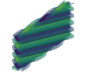
This section concludes with a brief description of the physical features of the perturbation fields. Figure 10 displays the optimal perturbation fields of a typical growing disturbance for  $R = 5$, $M=1$, $m = 0.05$ and $\tau _0=10$, at initial time $\tau _0$ and at the time $\tau \approx 31.6$ when $G_T \approx 10$. The perturbation fields are characterized by flow patterns that are tilted against the base-flow shear, which persists throughout the linear amplification region considered here. This misalignment facilitates efficient energy transfer from the base flow to the perturbation (Farrell Reference Farrell1988; Schmid & Henningson Reference Schmid and Henningson2001; Foures et al. Reference Foures, Caulfield and Schmid2014). As time increases, the peak of $u_1$ shifts from the heavier (right) to the lighter (left) fluid region. Furthermore, the peaks of $w_1$ seem no longer concentrated around $\eta = 0$, but have developed more local peaks adjacent at both sides of the core mixing layer. Finally, both $w_1$ and scalar fields have changed their orientation and are now tilted opposite to their original alignments.

Figure 10. Two-dimensional optimal perturbation fields  $u_1$ (a,d), $w_1$ (b,e) and $Y_1$ (c, f) at initial time $\tau _0$ (a–c) and at time ( $\tau = 31.64$) when $G_{T} \approx 10$ (d–f) of typical growing disturbance for $R = 5$, $M=1$, $m = 0.05$ and $\tau _0=10$.
4.2. Three-dimensional perturbations
In this section we consider conditions close to the neutral amplification wavenumber where the perturbations are not expected to grow. The QSSA indicates that this happens at  $m_{neutral}=0.148$ for $R = 5$, $M = 1$ and $\tau _0 = 10$. Therefore, we choose $m = 0.16$, slightly higher than $m_{neutral}$, and first investigate the influence of different objective functions for fixed $k$. Figure 11 shows comparisons of the different amplification factors for $k=0.05$ and optimized solutions with cost functions $E_Y$, $E_K$ and $E_T$. Generally, we observe that $G_T$ (also $G_K$) is larger than $G_Y$, as before, but interestingly $G_T$ (also $G_K$) displays transient growth for all types of cost function optimization (Butler & Farrell Reference Butler and Farrell1992; Schmid & Henningson Reference Schmid and Henningson2001; Kaminski et al. Reference Kaminski, Caulfield and Taylor2014). The peak of this transient growth happens at approximately the same time (for different optimization functions) but the decay is substantially slower when using $E_Y$, followed by $E_T$ and much faster when using $E_K$. Evidently, the intermediate decay displayed by the $E_T$ optimization is a combination of the effects of purely optimizing on the scalar variance $E_Y$ (slower decay) and the kinetic energy of the flow $E_K$ (faster decay). The curves of $G_Y$ for all these cases show also transient behaviour but of different nature. When optimizing for $E_Y$ and $E_T$ (figure 11a,c), we observe an initial decay of the scalar variance, which was attributed earlier to diffusion. After this decay, which is not observed when optimizing $E_K$, there is transient growth towards a peak, followed by decay. In the optimized solutions using $E_Y$ and $E_T$, the scalar amplification factor never exceeds the initial scalar variance.

Figure 11. Optimal amplification factors  $G_T$, $G_K$ and $G_Y$ with different cost functions $E_Y$ (a), $E_K$ (b) and $E_T$ (c) for $R = 5$, $M = 1$, $\tau _0 = 10$, $m = 0.16$ and $k = 0.05$.
Now, we concentrate on optimized solutions with the total energy cost function,  $E_T$, since it encompasses both flow and scalar behaviour. Figure 12 displays the evolution of $G_T$ for different values of the spanwise wavenumber $k$. First, it is apparent that there is short-term transient growth at all $k$ plotted, with $G_{T,max}$ larger than that of the purely two-dimensional mode $k=0$. This can be attributed to the lift-up effect of fluid elements in shear flows (Schmid & Henningson Reference Schmid and Henningson2001). The behaviour of $G_{T,max}$ is not monotonic with $k$, however. Factor $G_{T,max}$ increases with increasing $k$ up to $k \approx 0.1$, followed by a decrease of the amplification factor for larger $k$. All perturbations eventually decay, with the two-dimensional mode experiencing the slowest rate of decay at large times, which indicates that three-dimensional modes are slightly more important early on during the evolution. Note that the differences in amplification factors are not large for all values of $k$ shown.

Figure 12. The  $E_T$-optimal amplification factors for $R=5$, $M=1$, $\tau _0 = 10$ and $m = 0.16$, and different values of $k$.
$k$.
Figure 13 shows the optimal perturbation fields for the two-dimensional case (corresponding to the black curve in figure 12) of  $R = 5$, $M=1$, $m = 0.16$ and $\tau _0=10$, at initial time $\tau _0$ and at the time ( $\tau = 15.52$) when maximum amplification is reached: $G_{T,max} \approx 2.53$. As seen before at lower $m$, initially the flow patterns are tilted slightly against the base-flow shear but, as time progresses, the disturbances eventually rotate to become more aligned with the mean shear direction and cause transient growth of energy, also known as the Orr mechanism (Schmid & Henningson Reference Schmid and Henningson2001). Overall, the behaviour is similar to that displayed by the perturbations at lower $m$ in figure 10.

Figure 13. Two-dimensional ( $k = 0$) optimal perturbation fields $u_1$ (a,d), $w_1$ (b,e) and $Y_1$ (c, f) at initial time $\tau _0$ (a–c) and at time ( $\tau = 15.52$) when $G_{T,max} \approx 2.53$ (d–f) for $R = 5$, $M=1$, $m = 0.16$ and $\tau _0=10$.
Finally, figure 14 shows the optimal perturbation fields for a three-dimensional case (corresponding to the green curve in figure 12) of  $R = 5$, $M=1$, $k = 0.05$, $m = 0.16$ and $\tau _0=10$, at the initial time (figure 14a,c,e,g) and at the time ( $\tau = 15.88$) when maximum amplification is reached (figure 14b,d, f,h): $G_{Y,max} \approx 2.69$. The perturbation patterns are similar to those of figure 13 except that the oblique structure of the mode is now evident. The presence of a spanwise component of perturbation $v_1$ is also worth mentioning, and noticing that it has magnitude similar to that of $u_1$.

Figure 14. Three-dimensional optimal perturbation fields  $u_1$, $v_1$, $w_1$ and $Y_1$ at $\tau _0=10$ (a,c,e,g) and $\tau =15.88$ (b,d, f,h) for $R = 5$, $M=1$, $k = 0.05$ and $m = 0.16$.
5. Comparison with DNS
The DNS study carried out by Gat et al. (Reference Gat, Matheou, Chung and Dimotakis2017) considered uniform viscosity,  $M = 1$, for several density ratios $R$. They analysed the behaviour of the thickness of the interface with time and other nonlinear statistics not covered in this study. Figure 15 displays the evolution of the shear-layer width, which indicates that there are two mixing-layer temporal evolution regimes: an initial diffusion-dominant regime with growth rate $\sim \sqrt {\tau }$, followed by a turbulence-dominated regime with growth rate $\sim \tau ^3$. The early-time growth corresponds to viscous spreading contained in the base (self-similar) profiles, whereas the growing disturbances which dominate the base flows promote much faster growth at later times, as described below.

Figure 15. Temporal evolution of the shear-layer width  $(\delta /\delta _i)\sqrt {t_i/T_{DNS}}$ including the base profile (a), and perturbation width excluding the base profile $(\delta _1/\delta _i)\sqrt {t_i/T_{DNS}}$ (b) for forward integrations with $R = 5$, $M = 1$, $\tau _0 = 1.12$ and several values of $m$, compared against DNS result taken from Gat et al. (Reference Gat, Matheou, Chung and Dimotakis2017).
In order to compare the DNS results with LSA, first one needs to translate the parameters of their initial conditions to the present variables. Defining the initial shear-layer thickness  $\delta _i$ as the width at which $0.1 < Y < 0.9$ at initial time $t_i$, from figure 3(b) of Gat et al. (Reference Gat, Matheou, Chung and Dimotakis2017) we obtain $\delta _i \approx 0.02\ell = 0.13$ for $R = 5$, where $\ell = 2{\rm \pi}$. Meanwhile, this corresponds to $\Delta \eta \approx 2.96$ in our self-similar $Y_0$ profile in figure 2. By using (2.7b) and (3.2), we can determine their initial (start-up) time, given in our non-dimensional units by
 \begin{align} \tau_0 = \left(\frac{\delta_i/L}{\Delta \eta}\right)^2 \frac{1}{2K} = \left[\frac{\delta_i/(\bar{\nu}^{2}g^{{-}1})^{1/3}}{\Delta \eta}\right]^2 \frac{R{\textit{Sc}}}{2(R+1)} = \left[\frac{0.13/(0.0044^{2/3})}{2.96}\right]^2 \frac{5}{12} = 1.12, \end{align}
for their given  $\mu = 0.0044$ and $g = 1$. Secondly, we need to match their perturbation wavenumber to our $m$. From figure 15(a) in Gat et al. (Reference Gat, Matheou, Chung and Dimotakis2017), for ‘Pert3’ on $1024^3$ grid, the dimensionless wavenumber corresponding to the peak of the perturbation spectrum is $k_r\Delta x \approx 0.15$, which yields $k_r \approx (0.15)(1024)/(4{\rm \pi} ) = 12.22$, since their domain size is $4{\rm \pi}$. We non-dimensionalize this result to obtain our $m_{peak} = k_r L = (12.22)(\bar {\nu }^{2}g^{-1})^{1/3} = 0.33$. Subsequently, we carry out forward integration for $R = 5$, $M = 1$, $\tau _0 = 1.12$ for several wavenumbers, starting from $m_{peak}$ down to its sixth subharmonics. Figure 15 shows the temporal evolutions of the shear-layer thickness $\delta$ (figure 15a) and the width of the perturbation $\delta _1$ (figure 15b) compared against the DNS from Gat et al. (Reference Gat, Matheou, Chung and Dimotakis2017). The horizontal axis is scaled with the time scale used in their simulation, $T_{DNS}$, given by
 \begin{equation} T_{DNS} = 2{\rm \pi} \sqrt{\frac{\ell}{\mathcal{A}g}} = 19.29, \quad \mbox{where} \ \mathcal{A} = \frac{R-1}{R+1} = \frac{2}{3} \quad \mbox{for} \ R = 5. \end{equation}
We observe that the transition from viscous decay to rapid growth happens at  $(t+t_i)/T_{DNS} \approx 0.1$. This is comparable with the transition times observed in the DNS given by $(t+t_i)/T_{DNS} \approx 0.25$. The slightly earlier transition time predicted by LSA owes its origin to the initial condition used in the linearized study, which is obtained from the eigenmodes of the QSSA analysis, since these modes are more unstable than the random two-dimensional field, with a wide spectrum, used in the DNS. Despite this difference, the agreement is quite good and helps to connect the linear and nonlinear studies. It appears that the peak wave mode chosen space between words in the DNS was not an amplifying one, and instead the instability was triggered by lower wave modes present in the initial condition.
6. Conclusion
The LSA of two fluid columns with different densities and viscosities in a gravitational field has been investigated and compared with previous inviscid analysis. In this configuration, a uniform gravity field acts in the direction transverse to the density stratification, resulting in opposing constant acceleration of the free streams. We perform numerical integration of the linear time-dependent IVP as a function of wavenumber. Furthermore, we carry out adjoint optimization in order to determine the initial profiles that result in maximum amplification at a finite time horizon. Within the strongly unstable range of wavenumbers, we confirm that the evolution approaches the inviscid limit as the initial Reynolds number of the flow increases. In this regime, the two-dimensional mode is the most unstable (dominant). At higher wave modes, around the region of neutral stability, it is found that transient growth is present and that three-dimensional modes (with a spanwise non-zero wavenumber) are more unstable than the two-dimensional mode. The difference in amplification factors between two- and three-dimensional modes is not very large, but it is noticeable.
We also investigated the effect of different optimization cost functions and concluded that using the total energy of the flow, kinetic and potential, gives an overall picture of the evolution. Using a cost function based only on scalar variance (potential energy) highlights initial transients of the mixture fraction that are controlled by diffusion. Optimization of the initial scalar profiles can largely remove this diffusional decay from the dynamics but hides flow effects (velocity) that are important overall.
Funding
This work was supported in part by the Department of Energy, National Nuclear Security Administration, under award no. DE-NA0002382, and the California Institute of Technology. Computational resources were provided by the University of Southern California's Center for Advanced Research Computing.
Declaration of interests
The authors report no conflict of interest.
Appendix A. Detailed perturbation equations
A.1. Linear IVP – forward equations
The forward equations for the first-order perturbation fields are
 \begin{align}
\frac{\partial \hat{U}}{\partial \tau} &=
\frac{{\textit{Sc}} \mu_0 Z_0}{2\tau} D^2\hat{U} +
\left\{\frac{[(R-1)\mu_0 + 2 \beta{\textit{Sc}}
Z_0 ]Y_{0}' + 2 \eta}{4\tau}\right\}
D\hat{U}\nonumber\\ &\quad -\left[\mathrm{i} (k V_0 +
m W_0 \tau) + \frac{(k^2 +
m^2){\textit{Sc}} K\mu_0 Z_0}{2}
-\frac{(R-1)(\mu_0 Y_{0}'' + \beta
Y_0^{'2})}{4\tau}\right]\hat{U} \nonumber\\ &\quad +
\frac{\mathrm{i} k B\mu_0 Z_0 }{\sqrt{\tau}} D\hat{V} +
\frac{\mathrm{i}m B\mu_0 Z_0}{\sqrt{\tau}} D\hat{W} -
\frac{\beta (R-1) B Z_0(\mu_0 Y''_0 + \beta
Y_0^{'2})}{2 \sqrt{\tau^3}} D\hat{Y} \nonumber\\
&\quad + \left[\frac{\mathrm{i}(k V'_0 + m W'_0 \tau
)\beta B Z_0 }{\sqrt{\tau}} +
\frac{\left(R-1\right)^2B(\mu_0^2 Y'''_0 + 4 \beta
\mu_0 Y'_0Y''_0 +
\beta^2Y_0^{'3})}{4{\textit{Sc}}\sqrt{\tau^3}}\right.
\nonumber\\ &\quad \left. - \frac{\beta(R-1)
BZ_0(\mu_0 Y'''_0 + 3 \beta Y'_0Y''_0 )
}{2\sqrt{\tau^3}} \right]\hat{Y} - \frac{BZ_0}{\sqrt{\tau}}
D\hat{P},
\end{align}
\begin{align}
\frac{\partial \hat{U}}{\partial \tau} &=
\frac{{\textit{Sc}} \mu_0 Z_0}{2\tau} D^2\hat{U} +
\left\{\frac{[(R-1)\mu_0 + 2 \beta{\textit{Sc}}
Z_0 ]Y_{0}' + 2 \eta}{4\tau}\right\}
D\hat{U}\nonumber\\ &\quad -\left[\mathrm{i} (k V_0 +
m W_0 \tau) + \frac{(k^2 +
m^2){\textit{Sc}} K\mu_0 Z_0}{2}
-\frac{(R-1)(\mu_0 Y_{0}'' + \beta
Y_0^{'2})}{4\tau}\right]\hat{U} \nonumber\\ &\quad +
\frac{\mathrm{i} k B\mu_0 Z_0 }{\sqrt{\tau}} D\hat{V} +
\frac{\mathrm{i}m B\mu_0 Z_0}{\sqrt{\tau}} D\hat{W} -
\frac{\beta (R-1) B Z_0(\mu_0 Y''_0 + \beta
Y_0^{'2})}{2 \sqrt{\tau^3}} D\hat{Y} \nonumber\\
&\quad + \left[\frac{\mathrm{i}(k V'_0 + m W'_0 \tau
)\beta B Z_0 }{\sqrt{\tau}} +
\frac{\left(R-1\right)^2B(\mu_0^2 Y'''_0 + 4 \beta
\mu_0 Y'_0Y''_0 +
\beta^2Y_0^{'3})}{4{\textit{Sc}}\sqrt{\tau^3}}\right.
\nonumber\\ &\quad \left. - \frac{\beta(R-1)
BZ_0(\mu_0 Y'''_0 + 3 \beta Y'_0Y''_0 )
}{2\sqrt{\tau^3}} \right]\hat{Y} - \frac{BZ_0}{\sqrt{\tau}}
D\hat{P},
\end{align} \begin{align}
\frac{\partial \hat{V}}{\partial \tau} &= \frac{\mathrm{i}k
B \mu_0 Z_0 }{\sqrt{\tau}} D\hat{U} +
\left(\frac{\mathrm{i}k \beta B Z_0
Y_{0}'}{\sqrt{\tau}}-\frac{V_{0}'}{\sqrt{2K\tau}}\right)
\hat{U} + \frac{{\textit{Sc}} \mu_0 Z_0}{4\tau}
D^2\hat{V}\nonumber\\ &\quad +
\left\{\frac{\left[\left(R-1\right)\mu_0 +
\beta{\textit{Sc}} Z_0 \right]Y_{0}' + 2
\eta}{4\tau}\right\} D\hat{V} \nonumber\\ &\quad -
\left[\mathrm{i} (k V_0 + m W_0 \tau) +
\frac{(2k^2 + m^2){\textit{Sc}} K\mu_0
Z_0}{2}\right]\hat{V} \nonumber\\ &\quad- \frac{k m
{\textit{Sc}} K \mu_0 Z_0}{2}\hat{W} +
\frac{\beta{\textit{Sc}} Z_0 V'_0}{4\tau} D\hat{Y}
+\frac{{\textit{Sc}}\left[\beta Z_0 V''_0 -
\left(R-1\right) \left( \mu_0V''_0 + \beta V'_0 Y'_0
\right)\right] }{4\tau} \hat{Y} \nonumber\\ &\quad -
\frac{\mathrm{i}k {\textit{Sc}} K Z_0}{2}\hat{P},
\end{align}
\begin{align}
\frac{\partial \hat{V}}{\partial \tau} &= \frac{\mathrm{i}k
B \mu_0 Z_0 }{\sqrt{\tau}} D\hat{U} +
\left(\frac{\mathrm{i}k \beta B Z_0
Y_{0}'}{\sqrt{\tau}}-\frac{V_{0}'}{\sqrt{2K\tau}}\right)
\hat{U} + \frac{{\textit{Sc}} \mu_0 Z_0}{4\tau}
D^2\hat{V}\nonumber\\ &\quad +
\left\{\frac{\left[\left(R-1\right)\mu_0 +
\beta{\textit{Sc}} Z_0 \right]Y_{0}' + 2
\eta}{4\tau}\right\} D\hat{V} \nonumber\\ &\quad -
\left[\mathrm{i} (k V_0 + m W_0 \tau) +
\frac{(2k^2 + m^2){\textit{Sc}} K\mu_0
Z_0}{2}\right]\hat{V} \nonumber\\ &\quad- \frac{k m
{\textit{Sc}} K \mu_0 Z_0}{2}\hat{W} +
\frac{\beta{\textit{Sc}} Z_0 V'_0}{4\tau} D\hat{Y}
+\frac{{\textit{Sc}}\left[\beta Z_0 V''_0 -
\left(R-1\right) \left( \mu_0V''_0 + \beta V'_0 Y'_0
\right)\right] }{4\tau} \hat{Y} \nonumber\\ &\quad -
\frac{\mathrm{i}k {\textit{Sc}} K Z_0}{2}\hat{P},
\end{align} \begin{align}
\frac{\partial \hat{W}}{\partial \tau} &= \frac{\mathrm{i}m
B\mu_0 Z_0 }{\sqrt{\tau}} D\hat{U} +
\left(\frac{\mathrm{i}m \beta B Z_0
Y_{0}'}{\sqrt{\tau}}-\sqrt{\frac{\tau}{2K}}W_0'\right)\hat{U}\nonumber\\
&\quad - \frac{k m{\textit{Sc}} K \mu_0 Z_0}{2}\hat{V}
+ \frac{{\textit{Sc}} \mu_0 Z_0}{4\tau} D^2 \hat{W} +
\left\{\frac{\left[\left(R-1\right)\mu_0 +
\beta{\textit{Sc}} Z_0 \right]Y_{0}' + 2 \eta}{4\tau}
\right\}D\hat{W} \nonumber\\ &\quad-\left[\mathrm{i}
(k V_0 + m W_0 \tau) + \frac{(k^2 +
2m^2){\textit{Sc}} K\mu_0 Z_0}{2}\right]\hat{W}
+ \frac{\beta{\textit{Sc}} Z_0 W'_0}{4}D\hat{Y}
\nonumber\\ &\quad +
\left\{\frac{{\textit{Sc}}\left[\beta Z_0 W''_0 -
\left(R-1\right) \left( \mu_0W''_0 + \beta W'_0 Y'_0
\right) \right]}{4} - \frac{R^2-1}{2R} \right\}\hat{Y} -
\frac{\mathrm{i}m{\textit{Sc}} K Z_0}{2}\hat{P},
\end{align}
\begin{align}
\frac{\partial \hat{W}}{\partial \tau} &= \frac{\mathrm{i}m
B\mu_0 Z_0 }{\sqrt{\tau}} D\hat{U} +
\left(\frac{\mathrm{i}m \beta B Z_0
Y_{0}'}{\sqrt{\tau}}-\sqrt{\frac{\tau}{2K}}W_0'\right)\hat{U}\nonumber\\
&\quad - \frac{k m{\textit{Sc}} K \mu_0 Z_0}{2}\hat{V}
+ \frac{{\textit{Sc}} \mu_0 Z_0}{4\tau} D^2 \hat{W} +
\left\{\frac{\left[\left(R-1\right)\mu_0 +
\beta{\textit{Sc}} Z_0 \right]Y_{0}' + 2 \eta}{4\tau}
\right\}D\hat{W} \nonumber\\ &\quad-\left[\mathrm{i}
(k V_0 + m W_0 \tau) + \frac{(k^2 +
2m^2){\textit{Sc}} K\mu_0 Z_0}{2}\right]\hat{W}
+ \frac{\beta{\textit{Sc}} Z_0 W'_0}{4}D\hat{Y}
\nonumber\\ &\quad +
\left\{\frac{{\textit{Sc}}\left[\beta Z_0 W''_0 -
\left(R-1\right) \left( \mu_0W''_0 + \beta W'_0 Y'_0
\right) \right]}{4} - \frac{R^2-1}{2R} \right\}\hat{Y} -
\frac{\mathrm{i}m{\textit{Sc}} K Z_0}{2}\hat{P},
\end{align}
 \begin{align} \frac{\partial \hat{Y}}{\partial \tau} &={-}\frac{Y_{0}'}{\sqrt{2K\tau}}\hat{U} + \frac{\mu_0 Z_0}{4\tau} D^2\hat{Y} + \left\{\frac{\left[\left(R-1\right) \mu_0 +2 \beta Z_0\right]Y_{0}'+ 2 \eta}{4\tau}\right\}D \hat{Y}\nonumber\\ &\quad -\left[ \mathrm{i} \left(k V_0 + m W_0 \tau\right) + \frac{(k^2 + m^2)K\mu_0 Z_0 }{2}+ \frac{(R-1)(\mu_0 Y_{0}'' + \beta Y_0^{'2}) - \beta Z_0 Y_{0}'' }{4\tau}\right]\hat{Y}, \end{align}
 \begin{align} &\frac{1}{\sqrt{2K\tau}}D\hat{U} + \mathrm{i}k\hat{V} + \mathrm{i}m\hat{W} \nonumber\\ &\quad + \left(R-1\right)\left\{\frac{\mu_0}{4\tau} D^2\hat{Y} + \frac{\beta Y'_0}{2\tau} D\hat{Y} + \left[\frac{\beta Y''_0}{4\tau} - \frac{(k^2 + m^2)K\mu_0}{2}\right]\hat{Y}\right\} = 0, \end{align}
where the symbols  $D$ and primes denote $\eta$-derivatives. The equations above can be expressed in compact form as
 $$\begin{gather} \frac{\partial \hat{\boldsymbol{X}}}{\partial \tau} = \boldsymbol{A}\hat{\boldsymbol{X}} + \boldsymbol{B}\hat{P}, \end{gather}$$
 $$\begin{gather}\boldsymbol{C}\hat{\boldsymbol{X}} = 0, \end{gather}$$
where  $\hat {\boldsymbol {X}} = ( \hat {U},\hat {V},\hat {W},\hat {Y})$. Taking the derivative of (A6b) with respect to time, we have
 \begin{equation} \frac{\partial \boldsymbol{C}}{\partial \tau}\hat{\boldsymbol{X}}+ \boldsymbol{C}\frac{\partial \hat{\boldsymbol{X}}}{\partial \tau} = 0, \end{equation}
and substituting (A6a) yields the equation for pressure:
 \begin{equation} \hat{P} ={-}\left(\boldsymbol{C}\boldsymbol{B}\right)^{{-}1}\left(\frac{\partial \boldsymbol{C}}{\partial \tau} + \boldsymbol{C}\boldsymbol{A}\right)\hat{\boldsymbol{X}}. \end{equation}
The pressure can be substituted back into (A6a) to obtain
 \begin{equation} \frac{\partial \hat{\boldsymbol{X}}}{\partial \tau} = \left[\boldsymbol{A} - \boldsymbol{B}\left(\boldsymbol{C}\boldsymbol{B}\right)^{{-}1}\left(\frac{\partial \boldsymbol{C}}{\partial \tau} + \boldsymbol{C}\boldsymbol{A}\right)\right]\hat{\boldsymbol{X}} \equiv \boldsymbol{L} \hat{\boldsymbol{X}}. \end{equation}
In the numerical implementation, after performing the spatial discretization (as described in § 3.1), the implicit second-order Crank–Nicolson time-marching method has the form of
 $$\begin{gather} \frac{\hat{\boldsymbol{X}}^{n+1} - \hat{\boldsymbol{X}}^{n}}{\varDelta \tau} = \frac{1}{2}[\mathbb{A}^{n}\,\hat{\boldsymbol{X}}^{n} + \mathbb{A}^{n+1}\,\hat{\boldsymbol{X}}^{n+1}] + \mathbb{B}^{n+1/2}\,\hat{P}^{n+1/2}, \end{gather}$$
 $$\begin{gather}\mathbb{C}^{n+1}\,\hat{\boldsymbol{X}}^{n+1} = 0, \end{gather}$$
where the block matrices  $\mathbb {A}$, $\mathbb {B}$ and $\mathbb {C}$ are the discrete counterparts of those in (A6). Rearranging terms, we have
 \begin{equation}
\left[ \begin{matrix} \mathbb{E} & \mathbb{F}\\
\displaystyle \mathbb{C} & 0 \end{matrix} \right]
\left[\begin{matrix} \hat{\boldsymbol{X}}^{n+1} \\
\hat{P}^{n+1/2} \end{matrix} \right] =\left[\begin{matrix}
\mathbb{G}\hat{\boldsymbol{X}}^{n} \\ 0 \end{matrix}
\right],
\end{equation}
\begin{equation}
\left[ \begin{matrix} \mathbb{E} & \mathbb{F}\\
\displaystyle \mathbb{C} & 0 \end{matrix} \right]
\left[\begin{matrix} \hat{\boldsymbol{X}}^{n+1} \\
\hat{P}^{n+1/2} \end{matrix} \right] =\left[\begin{matrix}
\mathbb{G}\hat{\boldsymbol{X}}^{n} \\ 0 \end{matrix}
\right],
\end{equation}
where  $\mathbb {E} = (\mathbb {I} - \Delta \tau \mathbb {A}^{n+1}/2)$, $\mathbb {F} = (-\Delta \tau \mathbb {B}^{n+1/2})$, $\mathbb {G} = (\mathbb {I} + \Delta \tau \mathbb {A}^{n}/2)$ and $\mathbb {I}$ is the identity block matrix. We apply Schur complement reduction to obtain
 \begin{equation}
\left[ \begin{matrix} \mathbb{E} & \mathbb{F}\\ 0 &
-\mathbb{C}\mathbb{E}^{{-}1}\mathbb{F} \end{matrix}
\right] \left[\begin{matrix} \hat{\boldsymbol{X}}^{n+1}
\\ \hat{P}^{n+1/2} \end{matrix} \right]
=\left[\begin{matrix} \mathbb{G}\hat{\boldsymbol{X}}^{n}
\\
-\mathbb{C}\mathbb{E}^{{-}1}\mathbb{G}\hat{\boldsymbol{X}}^{n}
\end{matrix} \right],
\end{equation}
\begin{equation}
\left[ \begin{matrix} \mathbb{E} & \mathbb{F}\\ 0 &
-\mathbb{C}\mathbb{E}^{{-}1}\mathbb{F} \end{matrix}
\right] \left[\begin{matrix} \hat{\boldsymbol{X}}^{n+1}
\\ \hat{P}^{n+1/2} \end{matrix} \right]
=\left[\begin{matrix} \mathbb{G}\hat{\boldsymbol{X}}^{n}
\\
-\mathbb{C}\mathbb{E}^{{-}1}\mathbb{G}\hat{\boldsymbol{X}}^{n}
\end{matrix} \right],
\end{equation}from which we can solve for pressure and subsequently velocity and scalar fields.

Figure 16. Imaginary frequency  $\omega _I$ as (a) a function of $R$ for $M = 1$ and $\tau _0 = 10$, (b) a function of $M$ for $R = 5$ and $\tau _0 = 10$ and (c) a function of $\tau _0$ for $R = 5$ and $M = 1$.

Figure 17. The eigenfunctions for  $R= 5$, $M = 1$, $\tau _0 = 10$ and $m = 0.05$.
A.2. Quasi-steady-state approximation
In the QSSA, the base profiles are assumed to be frozen at a time  $\tau _0 >0$, when they are then perturbed, and the disturbance quantities have the following forms:
 \begin{align} &(u_1,
v_1, w_1,Y_1,p_1) \nonumber\\ &\quad =
[\hat{U}\left(\eta,\tau_0\right),\hat{V}\left(\eta,\tau_0\right),\hat{W}\left(\eta,\tau_0\right),\hat{Y}\left(\eta,\tau_0\right),\hat{P}(\eta,\tau_0)]
\exp({\mathrm{i}(k y+ m z - \omega \tau)})+ \textrm{c.c.},
\end{align}
\begin{align} &(u_1,
v_1, w_1,Y_1,p_1) \nonumber\\ &\quad =
[\hat{U}\left(\eta,\tau_0\right),\hat{V}\left(\eta,\tau_0\right),\hat{W}\left(\eta,\tau_0\right),\hat{Y}\left(\eta,\tau_0\right),\hat{P}(\eta,\tau_0)]
\exp({\mathrm{i}(k y+ m z - \omega \tau)})+ \textrm{c.c.},
\end{align}
where  $\omega$ $= \omega _{R} + \mathrm {i}\,\omega _{I}$, the imaginary part of which indicates temporal perturbation growth rate. This results in a generalized eigenvalue problem with $\tau = \tau _0$ as a parameter (Tan & Homsy Reference Tan and Homsy1986), which is then solved with the QZ algorithm (Corbett & Bottaro Reference Corbett and Bottaro2000). The results presented below are for two-dimensional cases ( $k = 0$) since $\omega _{I,2D} > \omega _{I,3D}$ for all cases. Figure 16(a) displays the imaginary amplification frequency $\omega _{I}(R,m)$ for uniform viscosity ratio $M=1$ and $\tau _0 = 10$, where $\omega _I$ increases with increasing $R$. Next, figure 16(b) shows $\omega _{I}(M,m)$ for density ratio $R=5$ and $\tau _0 = 10$, where the largest $\omega _I$ is achieved at the lowest $M$. Furthermore, figure 16(c) shows $\omega _{I}(\tau _0,m)$ for density ratio $R=5$ and uniform viscosity $M = 1$ as a function of $\tau _0$. For the largest $\tau _0 = 50$ case considered here, the peak growth rate is the highest among all, but the range of wavenumber $m$ at which $\omega _{I} >0$ is the narrowest. The opposite trend is observed at smallest $\tau _0$, where the positive growth rate is seen across a wider range of $m$, but the peak $\omega _{I}$ is the lowest. Finally, figure 17 displays the typical eigenfunctions obtained from QSSA for $R = 5$, $M = 1$, $\tau _0=10$ and $m = 0.05$, which are utilized as initial conditions for the forward integration.
A.3. Linear IVP – adjoint equations
The corresponding adjoint equations are
 \begin{align} &D\left(\frac{B Z_0}{\sqrt{\tau^+}}\hat{U}^+ \right) + \frac{\mathrm{i}k{\textit{Sc}} K Z_0}{2} V^+{+} \frac{\mathrm{i}m{\textit{Sc}} K Z_0}{2}\hat{W}^+{=} 0 , \end{align}
 \begin{align} \frac{\partial \hat{U}^+}{\partial \tau^+} &= D^2\left(\frac{{\textit{Sc}} \mu_0 Z_0 }{2\tau^+} \hat{U}^+\right) - D\left\{\frac{\left[(R-1)\mu_0 + 2\beta {\textit{Sc}} Z_0 \right]Y_{0}' + 2 \eta}{4\tau^+} \hat{U}^+ \right\} \nonumber\\ &\quad+\left[\mathrm{i} (k V_0 + m W_0 \tau^+) - \frac{(k^2 + m^2){\textit{Sc}} K\mu_0 Z_0}{2} +\frac{(R-1)(\mu_0 Y_{0}'' + \beta Y_0^{'2})}{4\tau^+}\right]\hat{U}^+ \nonumber\\ &\quad+ D\left(\frac{\mathrm{i} kB\mu_0 Z_0 }{\sqrt{\tau^+}} \hat{V}^+\right) - \left(\frac{\mathrm{i}k \beta B Z_0 Y_{0}'}{\sqrt{\tau^+}}+\frac{V_{0}'}{\sqrt{2K\tau^+}}\right)V^+{+} D\left(\frac{\mathrm{i}mB\mu_0 Z_0 }{\sqrt{\tau^+}} \hat{W}^+\right) \nonumber\\ &\quad - \left(\frac{\mathrm{i}m \beta B Z_0 Y_{0}'}{\sqrt{\tau^+}}+\sqrt{\frac{\tau^+}{2K}}W_{0}'\right)\hat{W}^+{-}\frac{Y_{0}'}{\sqrt{2K\tau^+}}\hat{Y}^+{-} \frac{1}{\sqrt{2K\tau^+}}D\hat{P}^+, \end{align}
 \begin{align}
\frac{\partial V^+}{\partial \tau^+} &=
D\left(\frac{\mathrm{i} k B\mu_0 Z_0 }{\sqrt{\tau^+}}
\hat{U}^+\right) + D^2 \left(\frac{{\textit{Sc}} \mu_0
Z_0}{4\tau^+} V^+\right) \nonumber\\
&\quad - D\left\{ \frac{\left[(R-1)\mu_0 +
\beta {\textit{Sc}} Z_0 \right]Y_{0}' + 2
\eta}{4\tau^+} V^+\right\} \nonumber\\ &\quad +
\left[\mathrm{i} (k V_0 + m W_0 \tau^+) - \frac{(2k^2
+ m^2){\textit{Sc}} K\mu_0 Z_0}{2}\right]V^+{-}
\frac{ k m {\textit{Sc}} K\mu_0 Z_0}{2} \hat{W}^+{-}
\mathrm{i}k\hat{P}^+,
\end{align}
\begin{align}
\frac{\partial V^+}{\partial \tau^+} &=
D\left(\frac{\mathrm{i} k B\mu_0 Z_0 }{\sqrt{\tau^+}}
\hat{U}^+\right) + D^2 \left(\frac{{\textit{Sc}} \mu_0
Z_0}{4\tau^+} V^+\right) \nonumber\\
&\quad - D\left\{ \frac{\left[(R-1)\mu_0 +
\beta {\textit{Sc}} Z_0 \right]Y_{0}' + 2
\eta}{4\tau^+} V^+\right\} \nonumber\\ &\quad +
\left[\mathrm{i} (k V_0 + m W_0 \tau^+) - \frac{(2k^2
+ m^2){\textit{Sc}} K\mu_0 Z_0}{2}\right]V^+{-}
\frac{ k m {\textit{Sc}} K\mu_0 Z_0}{2} \hat{W}^+{-}
\mathrm{i}k\hat{P}^+,
\end{align} \begin{align} \frac{\partial \hat{W}^+}{\partial \tau^+} &= D\left(\frac{\mathrm{i} m B\mu_0 Z_0 }{\sqrt{\tau^+}} \hat{U}^+\right) - \frac{k m {\textit{Sc}} K \mu_0 Z_0}{2}V^+{+} D^2 \left(\frac{{\textit{Sc}} \mu_0 Z_0}{4\tau^+} \hat{W}^+\right) \nonumber\\ &\quad - D\left\{ \frac{\left[(R-1)\mu_0 + \beta {\textit{Sc}} Z_0 \right]Y_{0}' + 2 \eta}{4\tau^+} W^+\right\} \nonumber\\ &\quad + \left[\mathrm{i} (k V_0 + m W_0 \tau^+) - \frac{(k^2 + 2m^2){\textit{Sc}} K\mu_0 Z_0}{2}\right]W^+{-}\mathrm{i}m \hat{P}^+, \end{align}
 \begin{align}
\frac{\partial \hat{Y}^+}{\partial \tau^+} &=
D\left[\frac{\beta(R-1) B Z_0(\mu_0 Y''_0 + \beta
Y_0^{'2})}{2 \sqrt{(\tau^{+})^3}} \hat{U}^+\right] -
\left[\frac{\mathrm{i}(k V'_0 + m W'_0 \tau^+)\beta B Z_0
}{\sqrt{\tau^+}}\right. \nonumber\\ &\quad
-\frac{(R-1)^2B(\mu_0^2 Y'''_0 + 4 \beta \mu_0
Y'_0Y''_0 +
\beta^2Y_0^{'3})}{4{\textit{Sc}}\sqrt{(\tau^+)^3}}\notag\\
&\quad
+ \left.\frac{\beta(R-1) BZ_0(\mu_0 Y'''_0 + 3 \beta
Y'_0Y''_0 ) }{2\sqrt{(\tau^+)^3}} \right]\hat{U}^+
\nonumber\\ &\quad - D\left(\frac{\beta{\textit{Sc}}
Z_0 V'_0 }{4\tau^+} V^+\right) +
\frac{{\textit{Sc}}[\beta Z_0 V''_0 - (R-1)
( \mu_0V''_0 + \beta V'_0 Y'_0
)]}{4\tau^+} V^+ \nonumber\\ &\quad -D \left(
\frac{ \beta {\textit{Sc}} Z_0 W'_0}{4} \hat{W}^+
\right)\notag\\
&\quad + \left\{\frac{{\textit{Sc}}\left[\beta Z_0
W''_0 - (R-1) \left( \mu_0W''_0 + \beta W'_0 Y'_0 \right)
\right]}{4} - \frac{R^2-1}{2R} \right\}\hat{W}^+
\nonumber\\ &\quad+ D^2 \left(\frac{\mu_0 Z_0}{4\tau^+}
\hat{Y}^+\right) - D\left\{ \frac{\left[(R-1) \mu_0 +2
\beta Z_0\right]Y_{0}'+ 2 \eta}{4\tau^+} \hat{Y}^+
\right\}\nonumber\\ &\quad +\left[ \mathrm{i} (k V_0 + m
W_0 \tau^+) - \frac{(k^2 + m^2)K\mu_0 Z_0}{2}\right.\notag\\
&\quad +\left. \frac{\beta
Z_0 Y_{0}'' - (R-1)(\mu_0 Y_{0}'' + \beta
Y_0^{'2}) }{4\tau^+}\right]\hat{Y}^+ \nonumber\\
&\quad + (R-1)\left\{D^2\left(
\frac{\mu_0}{4\tau^+}\hat{P}^+ \right) - D
\left(\frac{\beta Y'_0}{2\tau^+} \hat{P}^+ \right) +
\left[\frac{\beta Y''_0}{4\tau^+} - \frac{(k^2 +
m^2)K\mu_0}{2}\right] \hat{P}^+\right\}.
\end{align}
\begin{align}
\frac{\partial \hat{Y}^+}{\partial \tau^+} &=
D\left[\frac{\beta(R-1) B Z_0(\mu_0 Y''_0 + \beta
Y_0^{'2})}{2 \sqrt{(\tau^{+})^3}} \hat{U}^+\right] -
\left[\frac{\mathrm{i}(k V'_0 + m W'_0 \tau^+)\beta B Z_0
}{\sqrt{\tau^+}}\right. \nonumber\\ &\quad
-\frac{(R-1)^2B(\mu_0^2 Y'''_0 + 4 \beta \mu_0
Y'_0Y''_0 +
\beta^2Y_0^{'3})}{4{\textit{Sc}}\sqrt{(\tau^+)^3}}\notag\\
&\quad
+ \left.\frac{\beta(R-1) BZ_0(\mu_0 Y'''_0 + 3 \beta
Y'_0Y''_0 ) }{2\sqrt{(\tau^+)^3}} \right]\hat{U}^+
\nonumber\\ &\quad - D\left(\frac{\beta{\textit{Sc}}
Z_0 V'_0 }{4\tau^+} V^+\right) +
\frac{{\textit{Sc}}[\beta Z_0 V''_0 - (R-1)
( \mu_0V''_0 + \beta V'_0 Y'_0
)]}{4\tau^+} V^+ \nonumber\\ &\quad -D \left(
\frac{ \beta {\textit{Sc}} Z_0 W'_0}{4} \hat{W}^+
\right)\notag\\
&\quad + \left\{\frac{{\textit{Sc}}\left[\beta Z_0
W''_0 - (R-1) \left( \mu_0W''_0 + \beta W'_0 Y'_0 \right)
\right]}{4} - \frac{R^2-1}{2R} \right\}\hat{W}^+
\nonumber\\ &\quad+ D^2 \left(\frac{\mu_0 Z_0}{4\tau^+}
\hat{Y}^+\right) - D\left\{ \frac{\left[(R-1) \mu_0 +2
\beta Z_0\right]Y_{0}'+ 2 \eta}{4\tau^+} \hat{Y}^+
\right\}\nonumber\\ &\quad +\left[ \mathrm{i} (k V_0 + m
W_0 \tau^+) - \frac{(k^2 + m^2)K\mu_0 Z_0}{2}\right.\notag\\
&\quad +\left. \frac{\beta
Z_0 Y_{0}'' - (R-1)(\mu_0 Y_{0}'' + \beta
Y_0^{'2}) }{4\tau^+}\right]\hat{Y}^+ \nonumber\\
&\quad + (R-1)\left\{D^2\left(
\frac{\mu_0}{4\tau^+}\hat{P}^+ \right) - D
\left(\frac{\beta Y'_0}{2\tau^+} \hat{P}^+ \right) +
\left[\frac{\beta Y''_0}{4\tau^+} - \frac{(k^2 +
m^2)K\mu_0}{2}\right] \hat{P}^+\right\}.
\end{align}The equations above can be expressed in compact form as
 $$\begin{gather} \frac{\partial \hat{\boldsymbol{X}}^+}{\partial \tau^+} = \boldsymbol{A}^+\hat{\boldsymbol{X}}^+{+} \boldsymbol{B}^+\hat{P}^+, \end{gather}$$
 $$\begin{gather}\boldsymbol{C}^+\hat{\boldsymbol{X}}^+{=} 0, \end{gather}$$
where  $\hat {\boldsymbol {X}}^+ = (\hat {U}^+,\hat {V}^+,\hat {W}^+,\hat {Y}^+)$. Taking the derivative of (A19b) with respect to time, we have
 \begin{equation} \frac{\partial \boldsymbol{C}^+}{\partial \tau^+}\hat{\boldsymbol{X}}^+{+} \boldsymbol{C}^+\frac{\partial \hat{\boldsymbol{X}}^+}{\partial \tau^+} = 0, \end{equation}
and substituting (A19a) yields the equation for pressure:
 \begin{equation} \hat{P}^+{=} -\left(\boldsymbol{C}^+\boldsymbol{B}^+\right)^{{-}1}\left(\frac{\partial \boldsymbol{C}^+}{\partial \tau^+} + \boldsymbol{C}^+\boldsymbol{A}^+\right)\hat{\boldsymbol{X}}^+. \end{equation}
The pressure can be substituted back into (A19a) to obtain
 \begin{equation} \frac{\partial \hat{\boldsymbol{X}}^+}{\partial \tau^+} = \left[\boldsymbol{A}^+{-} \boldsymbol{B}^+\left(\boldsymbol{C}^+\boldsymbol{B}^+\right)^{{-}1}\left(\frac{\partial \boldsymbol{C}^+}{\partial \tau^+} + \boldsymbol{C}^+\boldsymbol{A}^+\right)\right]\hat{\boldsymbol{X}}^+{\equiv} \boldsymbol{L}^+ \hat{\boldsymbol{X}}^+. \end{equation}
Appendix B. Inviscid solution for non-zero velocity difference  $\Delta w_0$ at $t = t_0 > 0$


We generalize the inviscid formulation in Prathama & Pantano (Reference Prathama and Pantano2017) to account for a non-zero vertical velocity difference between the two streams in the  $z$ direction, $\Delta w_0$, at $t = t_0 > 0$, when the infinitesimal perturbation is initially imposed on the base flow. Prior to that, i.e. when $t < t_0$, it is assumed that the base flow is not perturbed. Denoting $\pm$ as the right and left fields with respect to the interface, respectively, the general structure of the equations for perturbation velocities is of the form
 \begin{equation} \frac{\partial \hat{\phi}^\pm}{\partial t} \pm \mathrm{i} m w_0^{{\pm}}(t) \hat{\phi}^\pm{=} C_0^\pm(t), \end{equation}
where
 \begin{equation} w_0^{{\pm}}(t) ={\mp} 2 a^{{\pm}}t, \quad a^{{\pm}} = \frac{R-1}{4R^{{\pm}}}g, \quad R^+{=} R, \quad R^-{=} 1, \end{equation}
and  $C_0^\pm (t)$ is the coefficient for the perturbation pressure, whose solution is
 \begin{equation} \hat{p}^\pm{=} C_0^\pm(t) \textrm{e}^{{\mp} \mathcal{K}x}, \end{equation}
where  $\mathcal {K}^2 = k^2 + m^2$. The relations between $\hat {\phi }^\pm$ and the perturbation velocities are given by
 \begin{equation} \hat{u}^\pm{=} \pm \frac{\mathcal{K}}{\rho^\pm} \hat{\phi}^\pm \textrm{e}^{{\mp} \mathcal{K}x} , \quad \hat{v}^\pm{=}{-} \frac{\mathrm{i}k}{\rho^\pm}\hat{\phi}^\pm \textrm{e}^{{\mp} \mathcal{K}x}, \quad \hat{w}^\pm{=}{-} \frac{\mathrm{i}m}{\rho^\pm}\hat{\phi}^\pm \textrm{e}^{{\mp} \mathcal{K}x}. \end{equation}
Solving (B1) with initial time  $t_0 > 0$, we obtain
 \begin{equation} \hat{\phi}^\pm(t)= \hat{\phi}_0^\pm \exp({\pm \mathrm{i} m a^\pm (t^2-t_0^2)}) + \int_{t_0}^{t} C_0^\pm(t') \exp({\pm \mathrm{i} m a^\pm(t^2-t'^2 )})\,\textrm{d}t'. \end{equation}
 Following Prathama & Pantano (Reference Prathama and Pantano2017), the differential equation for the interface amplitude  $\hat {\zeta }$ is given by
 \begin{align} &\frac{\partial \hat{\zeta}}{\partial t} \mp 2 \mathrm{i} m a^\pm t\hat{\zeta} = \hat{u}^\pm(x=0)\nonumber\\ &\quad ={\pm} \frac{\mathcal{K}}{\rho^\pm}\left[\hat{\phi}_0^\pm \exp({\pm \mathrm{i} m a^\pm (t^2-t_0^2)}) + \int_{t_0}^{t} C_0^\pm(t') \exp({\pm \mathrm{i} m a^\pm(t^2-t'^2)})\,\textrm{d}t'\right], \end{align}
and for zero surface tension,  $C_0^+(t) = C_0^-(t)$. Multiplying (B6) by $\exp ({\mp \mathrm {i} m a^\pm t^2})$, taking the derivative with respect to time, cancelling exponential terms on both sides and eliminating $C_0^\pm$, we obtain
 \begin{equation} \frac{\textrm{d}^2\hat{\zeta}}{\textrm{d}t^2} - \frac{\omega^4_0}{4}t^2 \hat{\zeta}(t) = 0, \end{equation}
with
 \begin{equation} \omega^4_0 = g^2 m^2 \frac{(R-1)^2}{R}. \end{equation}
Equation (B7a) can be non-dimensionalized by introducing  $\tilde {\tau } \equiv \omega _0 t$, giving
 \begin{equation} \frac{\textrm{d}^2\tilde{\zeta}}{\textrm{d}\tilde{\tau}^2} - \frac{\tilde{\tau}^2 }{4} \tilde{\zeta}= 0. \end{equation}
The general solution of (B8) can be expressed as
 \begin{equation} \tilde{\zeta}(\tilde{\tau}) = C_1 D_{{-}1/2}(\tilde{\tau}) + C_2 D_{{-}1/2}(\mathrm{i} \tilde{\tau}), \end{equation}
where  $D_j(z)$ denotes the parabolic cylinder function of order $j$. We require two initial conditions, the first of which is unity interface amplitude $\tilde {\zeta }(\tilde {\tau } = \tilde {\tau }_0)=1$. The other condition is $\tilde {\zeta }_{\tilde {\tau }}(\tilde {\tau } = \tilde {\tau }_0)=0$, obtained from setting $t = t_0$ in (B6) and choosing $\hat {\phi }_0^\pm$ such that the following condition is satisfied:
 \begin{equation} \mp 2 \mathrm{i} m a^\pm t_0 ={\pm} \frac{\mathcal{K}}{\rho^\pm}\hat{\phi}_0^\pm. \end{equation}
Finally, the constants are given by
 \begin{equation} C_1 = \frac{\tilde{\tau}_0D_{{-}1/2}(\mathrm{i}\tilde{\tau}_0)+2\mathrm{i}D_{1/2}(\mathrm{i}\tilde{\tau}_0)}{2C_3} \end{equation}
and
 \begin{equation} C_2 = \frac{\tilde{\tau}_0D_{{-}1/2}(\tilde{\tau}_0)-2D_{1/2}(\tilde{\tau}_0)}{2C_3}, \end{equation}
where
 \begin{equation} C_3 = \mathrm{i}D_{{-}1/2}(\tilde{\tau}_0)D_{1/2}(\mathrm{i}\tilde{\tau}_0) + D_{{-}1/2}(\mathrm{i}\tilde{\tau}_0)\left[\tilde{\tau}_0D_{{-}1/2}(\tilde{\tau}_0)-D_{1/2}(\tilde{\tau}_0)\right]. \end{equation}


 Open access