


1. Introduction
Vortex filaments are ubiquitous in nature, with helical vortex the simplest vortex filament that has both curvature and torsion. In terms of application, tip vortices generated in rotating devices such as propellers and helicopters can generally be modelled as helical vortices. In infinite ideal fluid, a helical vortex is one of only a few geometries that would translate/rotate due to self-induction without change of form (Levy & Forsdyke Reference Levy and Forsdyke1928). Consequently, the general stability of a helical vortex filament is a subject of fundamental scientific interest and practical importance.
Existing studies of helical vortex stability are mostly for unbounded fluid without boundary effects. Levy & Forsdyke (Reference Levy and Forsdyke1928) analysed the stability of a helical vortex with small core radius in infinite fluid, where the effect of entire perturbed filament on vortex self-induced motion is considered. However, they failed to obtain any meaningful results of vortex instability (due to a sign error in their final equations). Betchov (Reference Betchov1965) studied the same problem but used a simplified local-induction model, in which the self-induced velocity at any point on the vortex is proportional to local curvature and in the direction of the local binormal. It is found that the vortex filament is unstable to perturbation modes with wavenumber smaller than the local curvature. Using the cut-off regularisation method, Widnall (Reference Widnall1972) studied the stability of helical vortex filament of finite core. Three distinct modes of instability were found corresponding to short-wave mode, low-wavenumber mode and mutual inductance mode for small helical pitch. Taking the flow field inside the vortex core into account, Hattori & Fukumoto (Reference Hattori and Fukumoto2009) studied the stability of a helical vortex tube in the short-wave limit, where the basic flow was solved by means of a perturbation expansion of the Euler equation. There has also been interest in the stability of multiple helical vortices. Gupta & Loewy (Reference Gupta and Loewy1974) extended the results of Levy & Forsdyke (Reference Levy and Forsdyke1928) and Widnall (Reference Widnall1972), and dealt with the stability of centreline perturbations of the helical vortices system. This has been further generalised to include the external flow field (Okulov Reference Okulov2004; Okulov & Sørensen Reference Okulov and Sørensen2007), where the influence of prescribed flows on stability of multiple helical tip vortices was studied.
The theme of this work is the stability of a single helical vortex filament of infinite extent under a free surface. The presence of the free surface boundary can significantly modify the equilibrium configuration and influence the instability of the vortex filament in contrast to that in infinite fluid. The elucidation of the similarities and distinctions and the comparisons between the problems with the rigid wall boundary vs free surface is the main focus of the present work. Under the assumption of ideal fluid, we take into account the leading-order interaction effect between the vortex and the boundary upon the induced fluid motion, and analytically derive the modified equilibrium form, on which we perform linear stability analysis. Depending on the Froude number  $F_r$, the instability results can be characteristically different. In the case of rigid wall corresponding to $F_r \rightarrow 0$, the boundary effect can stabilise (or destabilise) the vortex to relatively long- (or short-)wavelength sub-harmonic displacement perturbations compared with the well-known stability result in infinite fluid. In the case of $F_r > 0$, surface waves are induced by the vortex. In contrast to the $F_r \rightarrow 0$ case, the wave effect destabilises the vortex to super-harmonic and long-wavelength sub-harmonic perturbations.
We organise the remainder of the paper as follows. In § 2, we state the specific problem to be investigated and define the key dimensionless parameters. We outline in § 3 the analytic approach on the determination of equilibrium form and linear stability analysis of a helical vortex under the influence of rigid boundary and free-surface wave effects. Section 4 gives a summary of the fluid particle velocities on the vortex filament induced by the primary vortex and its negative image about the mean free surface. The results of modified equilibrium form and stability analysis in the case of  $F_r \rightarrow 0$ (rigid wall) are presented and discussed in § 5. In the general free-surface case of $F_r > 0$, we describe the analytical solution of the linear wave field induced by the helical vortex in § 6, and present the equilibrium form and stability results in § 7. In § 8, we summarise our main findings.
2. Problem description
2.1. Problem definition and parameters
We consider a horizontal helical vortex of infinite extent, with helix radius  $a^*$, pitch $2{\rm \pi} b^*$, located at a (mean) submergence depth $h^* = a^* H \ (H > 1)$ from a free surface. The position of the undisturbed free surface is $z=0$, with gravity $g$ in the $-z$ direction. Referring to the definition sketch (figure 1), the centreline of the unperturbed vortex $\boldsymbol {X}_0^*(\theta )$ is located at
 \begin{equation} \boldsymbol{X}_0^*(\theta) = (x,y,z)(\theta) = (b^* \theta, a^* \cos\theta, a^* \sin\theta - h^*); \end{equation}
where  $\theta \in \mathbb {R}$ is the coordinate parameter. We assume that the vortex filament has a circular cross-section with (small) radius $e^* = a^* e_0$ ( $e_0 < 1$), within which the vorticity is uniformly distributed, parallel to the centreline tangent, and has total vortex circulation $\varGamma$. The flow outside is assumed irrotational.

Figure 1. Sketch of a helical vortex filament below a free surface.
We define  $L = b^*$, $U = \varGamma /(2{\rm \pi} L)$ and $T = L/U$ as the characteristic length, velocity and time scales, respectively. The problem is characterised by the non-dimensional geometry parameters: vortex radius $a = a^*/L$ (or slope $l = b^*/a^* = a^{-1}$ or helix angle $\vartheta = \arctan {(a)}$), core size $e = e^*/L = a e_0$, submergence $h = h^*/L = a H$; and the Froude number $F_r = U/\sqrt {g h^*}$ which measures the relative importance of free-surface deformation. For simplicity, we assume $e_0 \ll 1$ so that flow structure within the vortex tube can be neglected. Finally, for relatively weak interactions, and consistent with linearised wave theory, we assume $H \gg 1$ with the corresponding small parameter to be used in the analyses $\varepsilon \equiv 1/(2H)\ll 1$.
In what follows, we treat the cases of  $F_r \rightarrow 0$ and $F_r > 0$ separately. For $F_r \rightarrow 0$, surface wave effects can be neglected, and we focus on the effect of the vortex image, which is mainly controlled by the vortex submergence. The case of a helical vortex in the presence of a rigid wall is a special case of $F_r \rightarrow 0$ corresponding to the limit of $g \rightarrow \infty$ (for finite $h$). On the other hand, the case of a helical vortex in unbounded fluid is another special case of $F_r \rightarrow 0$ corresponding to the limit $h \rightarrow \infty$ (for given $g$). For $F_r > 0$, the main (additional) effect is the surface deformations induced by the vortex, and we focus on this wave effect upon the equilibrium form and stability of the underlying helical vortex.
2.2. Basic kinematics of a helical vortex filament in unbounded fluid
The self-induced motion of a helical vortex in unbounded fluid is well known (Levy & Forsdyke Reference Levy and Forsdyke1928; Boersma & Wood Reference Boersma and Wood1999; Fuentes Reference Fuentes2018). For later reference, we provide a brief summary and deduce some key results. For the helical vortex filament with geometry form (2.1), its non-dimensional translation velocity  $U_0$ and angular velocity $\varOmega _0$ are obtained from the Biot–Savart law and take the form
 \begin{equation} U_0 = \int_{0}^{\infty} a^2 (1-\cos\lambda) J_0^{{-}3/2}\, {\rm d} \lambda,\quad \varOmega_{0} = \int_{0}^{\infty} (1-\cos\lambda-\lambda\sin\lambda)J_0^{{-}3/2}\, {\rm d} \lambda, \end{equation}
in which  $J_0 = \lambda ^{2} + 2 a^{2} (1 - \cos \lambda ) + (a e_r)^2$ with the regularisation parameter $e_r = e_0 \, {\rm e}^{-3/4}$ (Fuentes Reference Fuentes2018). The non-dimensional time-dependent spatial position of the helical vortex is given by
 \begin{equation} \boldsymbol{X}_0(\theta,t) =(\theta + U_0 t, a \cos(\theta + \varOmega_0 t), a \sin(\theta + \varOmega_0 t) - h). \end{equation}
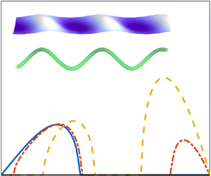
 Some profiles of  $U_0$ and $\varOmega _0$ for different helical vortex filaments are sketched in figure 2. As can be seen, the translation velocity $U_0$ and rotation velocity $\varOmega _0$ both weakly depend on vortex core size. In addition, from the inset of the right subplot, we see that $\varOmega _0$ changes sign as the helix radius increases for fixed core size, indicating that $\varOmega _0$ has certain zero points (Levy & Forsdyke Reference Levy and Forsdyke1928). This property is of importance when solving the new equilibrium configuration of vortex as discussed in § 5.1. The asymptotic solutions of $U_0$ and $\varOmega _0$ in the limits of small and large values of $a$, respectively, are derived from (2.2a,b) by the use of the method in Boersma & Wood (Reference Boersma and Wood1999) (see the supplementary material for details):
 \begin{equation} U_0 ={-} \frac{a^2\ln( a e_r )}{2(1+a^2)^{3/2}} + O(a^2), \quad \varOmega_0 = \frac{\ln( a e_r )}{2(1+a^2)^{3/2}} + \frac{1}{4}( 1 + 2\gamma - \ln4 ) + O(a^2), \end{equation}
as  $a \rightarrow 0$, and
 \begin{equation} U_0 = \frac{1}{2} - \frac{a^2 \ln( a e_r )}{2(1+a^2)^{3/2}} + O(a^{{-}3}), \quad \varOmega_0 = \frac{1}{2a^2} + \frac{\ln( a e_r )}{2(1+a^2)^{3/2}} + O(a^{{-}3}), \end{equation}
as  $a \rightarrow \infty$, where $\gamma \approx 0.577$ is the Euler constant.

Figure 2. Translation ( $U_0$) and rotation ( $\varOmega _{0}$) speeds of single helical vortex in infinite fluid.
Another interesting property of the single helical vortex is that the quantity  $C_0 \equiv U_0 - \varOmega _0$ is always positive. Physically, $C_0$ is related to $U_B$, the projection of the self-induced velocity of the vortex in the local bi-normal direction of the helix. It can be shown analytically (see the supplementary material for details) that
 \begin{equation} U_B = \frac{a}{\sqrt{1 + a^2}}(U_0 - \varOmega_{0}) > 0, \quad \forall \,a\in \mathbb{R}, e_0\in(0,1). \end{equation}
In addition,  $C_0$ represents the phase speed of waves induced by the helical vortex in the longitudinal direction, as described in § 6.
3. Equilibrium position and linear stability analysis
We outline the methodology and provide some general formulae for solving for the vortex equilibrium position and performing the linear stability analysis of the helical vortex in the presence of the boundary surface.
For vortex filament  $\boldsymbol {X}(\theta,t)$ submerged under a free surface, its motion is governed by the kinematic equation
 \begin{equation} \partial_t \boldsymbol{X}(\theta,t) = \boldsymbol{U}(\boldsymbol{X}(\theta,t),t), \end{equation}
where  $\boldsymbol {U}$ is the total velocity of the fluid particle on the vortex filament $\boldsymbol {X}(\theta,t)$. In the presence of a free surface, we decompose the total velocity into three components:
 \begin{equation} \boldsymbol{U}= \boldsymbol{U}_{{s}}+ \boldsymbol{U}_{{i}} + \boldsymbol{U}_{{w}} . \end{equation}
Here  $\boldsymbol {U}_{{s}}$ is the velocity field induced by the vortex $\boldsymbol {X}$ itself; $\boldsymbol {U}_{{i}}$ is the velocity field induced by its negative image $\tilde {\boldsymbol {X}}$, which is geometrically symmetric with $\boldsymbol {X}$ about the $z=0$ plane but with an opposite vortex circulation; and $\boldsymbol {U}_{{w}}$ is the wave induced velocity required to satisfy the (deformable) free-surface boundary condition for the general case of $F_r > 0$. In the limit $F_r \rightarrow 0$, the surface remains flat, $\boldsymbol {U}_{{w}}=0$, and $\boldsymbol {U}_{{s}}+ \boldsymbol {U}_{{i}}$ satisfies the required no-penetration condition on the boundary $z=0$.
3.1. Equilibrium configuration of vortex filament under a free surface
3.1.1. Representation of the equilibrium configuration
For any vortex filament  $\boldsymbol {X}(\theta,t)$ whose motion is governed by (3.1), we regard it as an equilibrium form if it moves without change of form in uniform translation. Thus, we look for vortex equilibrium form $\boldsymbol {X}(\theta, t)$ that satisfies
 \begin{equation} \exists \alpha \in \mathbb{R},\quad \boldsymbol{C}\in \mathbb{R}^3 \Longrightarrow \boldsymbol{X}(\theta,t) = \boldsymbol{X}(\theta + \alpha t, 0) + \boldsymbol{C} t, \quad \forall \, \theta \in \mathbb{R} , \end{equation}
where  $\alpha$ is an arbitrary constant and $\boldsymbol {C}$ is a constant translational velocity. This condition basically states that there is an (moving) inertial reference frame in which $\boldsymbol {X}(\theta,t)$ remains unchanged. As a special case, for example, the equilibrium configuration of the helical vortex in an infinite fluid is represented by (2.3) as $\boldsymbol {X}_0(\theta,t) = (\varphi, a\cos \varphi, a\sin \varphi - h ) + ( C_0,0,0) t$, with $\varphi = \theta + \varOmega _0 t$ and $C_0 = U_0 - \varOmega _0$.
The kinematic equation (3.1) is a nonlinear integro-differential equation and, in general, it is difficult to obtain an exact solution  $\boldsymbol {X}(\theta,t)$ that satisfies both (3.1) and (3.3). In this study, we seek approximate equilibrium solutions that are moderately perturbed from the helical vortex $\boldsymbol {X}_0$. We express the general equilibrium form of the vortex as
 \begin{equation} \boldsymbol{X}(\theta,t) =\boldsymbol{X}_0(\theta,t)+ \hat{\boldsymbol{r}}(\varphi) + \hat{\boldsymbol{u}} t, \quad \varphi \equiv \theta + \varOmega t,\ \varOmega \equiv \varOmega_0 + \hat{\omega}, \end{equation}
where  $\hat {\boldsymbol {r}}(\varphi )$ represents the geometric variation in the vortex filament, and $\hat {\boldsymbol {u}}$ and $\hat {\omega }$ are the changes in the translational velocity and rotational speed of the vortex, respectively, due to the presence of the (free) surface. In general $\hat {\boldsymbol {u}} = (\hat {u}, \hat {v}, \hat {w})$ can have three non-zero components. It will be shown in later sections that the induced velocity in the vertical direction $\hat {w}$ is negligibly small at the leading-order compared with $\hat {u}$ and $\hat {v}$. We thus assume $\hat {w} = 0$ and consider the vortex submergence $h$ to be fixed in the stability analysis. Like the geometric configuration of $\boldsymbol {X}_0$, $\hat {\boldsymbol {r}}(\varphi )$ is periodic in $\varphi$. We expand $\hat {\boldsymbol {r}}= (\hat {x}, \hat {y}, \hat {z})$ in Fourier series
 \begin{equation} \hat{\boldsymbol{r}}(\varphi) = \sum_{m{\neq}0} \hat{\boldsymbol{r}}_{m} \, {\rm e}^{{\rm j} m \varphi} = \sum_{m{\neq}0} ( \hat{x}_{m}, \hat{y}_{m}, \hat{z}_{m} ) \, {\rm e}^{{\rm j} m \varphi}, \end{equation}
where  ${\rm j}$ is the imaginary unit and $\hat {\boldsymbol {r}}_{m} = (\hat {x}_{m}, \hat {y}_{m}, \hat {z}_{m})$ represents the amplitude vector of the $m$th perturbation mode. Here the zeroth ( $m = 0$) mode is not taken into account because it simply represents a shift of origin of the coordinate system. As $\hat {\boldsymbol {r}}(\varphi )$ is real, we have $\hat {\boldsymbol {r}}_{-m} = \overline {\hat {\boldsymbol {r}}_{m}}$ for all $m\in \mathbb {N}$, where $\overline {(\ )}$ represents complex conjugate.
We exclude the trivial solutions of (3.1) by restricting the average modifications in both the radial and angular directions to be zero. The former constraint guarantees the helix radius  $a$ to be unaltered because any change in $a$ would be considered in the same stability analysis with different helix radius. The latter constraint excludes a phase shift along the helix tangent since it does not modify the geometric configuration of the helical vortex. These two constraints can be expressed in mathematical form as
 \begin{equation} \left\{\begin{array}{@{}l}\langle \hat{y} \cos\varphi + \hat{z} \sin\varphi \rangle = 0 \\ \langle \hat{y} \sin\varphi - \hat{z} \cos\varphi \rangle = 0 \end{array}\right. \quad \text{or} \quad \langle ( \hat{y} + {\rm j} \hat{z} ) \, {\rm e}^{-{\rm j} \varphi} \rangle = 0, \end{equation}
where  $\langle\, f \rangle$ denotes the mean value of the periodic function $f(\varphi )$ in the interval $[0, 2{\rm \pi} ]$.
For convenience in the analysis and description, we introduce the complex variable  $Y + {\rm j} Z$ to represent the $y$- and $z$-coordinates of the deformed helix $\boldsymbol {X}(\theta,t)=(X, Y, Z)(\theta,t)$. With this, we can express $\boldsymbol {X}(\theta,t)$ in a $2\times 1$ matrix form:
 \begin{equation} \begin{bmatrix} X \\ Y + {\rm j} Z \end{bmatrix} = \begin{bmatrix} \theta + U_0 t \\ a \, {\rm e}^{{\rm j} \varphi} - {\rm j} h \end{bmatrix} + \begin{bmatrix} \hat{u} \\ \hat{v} \end{bmatrix} t + \sum_{m\in\mathbb{Z}} \begin{bmatrix} - {\rm j} \hat{\chi}_{m} \\ \hat{\xi}_{m} \, {\rm e}^{{\rm j} \varphi} \end{bmatrix} \, {\rm e}^{{\rm j} m \varphi}, \end{equation}
with  $\varphi = \theta + \varOmega t$ and $\varOmega = \varOmega _0 + \hat {\omega }$. Here $\mathbb {Z}$ represents integers, $\hat {\chi }_{m} = {\rm j} \hat {x}_{m}$ and $\hat {\xi }_{m} = \hat {y}_{m+1} + {\rm j} \hat {z}_{m+1}$. In terms of $\hat {\chi }_{m}$ and $\hat {\xi }_{m}$, the constraints in (3.6) and the assumptions made on the vortex configuration $\boldsymbol {X}(\theta,t)$ can be expressed as
 \begin{equation} \hat{\chi}_{{-}m} ={-}\overline{\hat{\chi}_{m}} , \quad \hat{\chi}_{0} = \hat{\xi}_{0} = 0, \quad \hat{\xi}_{{-}1} = 0 . \end{equation}
3.1.2. Determination of the equilibrium configuration
We deduce here the governing equations for the unknown variables in the equilibrium form (3.7). To do this, we consider the leading-order terms in the motion equation (3.1), to then obtain the leading approximate solution of the vortex equilibrium form.
Similarly to  $\boldsymbol {X}(\theta,t)$, we expand the self-induced velocity along the vortex filament, $\boldsymbol {U}_{{s}}(\theta,t)=( U_{{s}}, V_{{s}}, W_{{s}})(\theta,t)$, in Fourier series:
 \begin{equation} U_{{s}} = U_0 + \sum_{m\in\mathbb{Z}} U_{{s},m} \, {\rm e}^{{\rm j} m \varphi}, \quad {\rm j} V_{{s}} - W_{{s}} ={-}a\varOmega_0 \, {\rm e}^{{\rm j} \varphi} + \sum_{m\in\mathbb{Z}} V_{{s},m} \, {\rm e}^{{\rm j} (m+1) \varphi}, \end{equation}
where the terms  $U_0$ and $-a\varOmega _0 \, {\rm e}^{{\rm j} \varphi }$ are due to the translational and rotational motions of the original helical vortex, respectively. Here $U_{{s},m}$ and $V_{{s},m}$ are the $m$th mode amplitudes of the induced velocity components associated with the modifications of the vortex configuration from the (free-surface) boundary effect. At the leading-order, they are linearly proportional to the $m$th Fourier mode amplitudes of the deformed equilibrium vortex configuration, $\hat {\chi }_m, \hat {\xi }_m$ and $\overline {\hat {\xi }_{-m}}$. For convenience in description, we express $U_{{s},m}$ and $V_{{s},m}$ in symbolic form
 \begin{equation} U_{{s},m} = \boldsymbol{A}_u(m) \boldsymbol{\cdot}\hat{\boldsymbol{R}}_{m}, \quad V_{{s},m} = \boldsymbol{A}_v(m) \boldsymbol{\cdot}\hat{\boldsymbol{R}}_{m} , \quad \hat{\boldsymbol{R}}_m = [ \hat{\chi}_{m}, \hat{\xi}_{m}, \overline{\hat{\xi}_{{-}m}} ]^{\rm T}, \end{equation}
where  $\boldsymbol {A}_u$ and $\boldsymbol {A}_v$ are the $1 \times 3$ coefficient vectors that depend on the mode number $m$ and vortex geometry parameters ( $a$ and $e_0$).
For the image-induced velocity  $\boldsymbol {U}_{{i}}=(U_{{i}}, V_{{i}}, W_{{i}} )$ and the wave-induced velocity $\boldsymbol {U}_{{w}}=(U_{{w}}, V_{{w}}, W_{{w}})$, under the assumption of $H \gg 1$, the leading-order contributions are from the original helical vortex whereas the effects of the modifications to the equilibrium vortex configuration are of higher order. As the modified helical configuration (and its image) is periodic in the longitudinal direction, both $\boldsymbol {U}_{{i}}$ and $\boldsymbol {U}_{{w}}$ are periodic in $\varphi$. (The proof of the periodicity of $\boldsymbol {U}_{{i}}$ is outlined in § 4.2). We expand the components of $\boldsymbol {U}_{{i}}$ and $\boldsymbol {U}_{{w}}$ in Fourier series and express them in symbolic form
 \begin{gather} U_{{i}} = \sum_{m\in\mathbb{Z}} U_{{i},m}(a, H) \, {\rm e}^{{\rm j} m \varphi}, \quad {\rm j} V_{{i}} - W_{{i}} = \sum_{m\in\mathbb{Z}} V_{{i},m}(a, H) \, {\rm e}^{{\rm j} (m+1) \varphi}, \end{gather}
 \begin{gather}U_{{w}} = \sum_{m\in\mathbb{Z}} U_{{w},m}(a, H, F_r) \, {\rm e}^{{\rm j} m \varphi}, \quad {\rm j} V_{{w}} - W_{{w}} = \sum_{m\in\mathbb{Z}} V_{{w},m}(a, H, F_r) \, {\rm e}^{{\rm j} (m+1) \varphi}, \end{gather}
where  $U_{{i},m}, V_{{i},m}, U_{{w},m}, V_{{w},m}$ are the associated $m$th Fourier mode amplitudes.
Upon substituting  $\boldsymbol {X}$ in (3.7), $\boldsymbol {U}_{{s}}$ in (3.9a,b), $\boldsymbol {U}_{{i}}$ in (3.11a,b) and $\boldsymbol {U}_{{w}}$ in (3.12a,b) into the motion equation (3.1) and matching the coefficients of each harmonic mode, we obtain
 \begin{gather} \boldsymbol{A}_u(m) \boldsymbol{\cdot}\hat{\boldsymbol{R}}_{m} - m \varOmega_0 \hat{\chi}_m - \hat{u} \delta_m ={-} U_{{i},m} - U_{{w},m}, \end{gather}
 \begin{gather}\boldsymbol{A}_v(m) \boldsymbol{\cdot}\hat{\boldsymbol{R}}_{m} + (m+1) \varOmega_0 \hat{\xi}_m - {\rm j} \hat{v} \delta_{m+1} + a \hat{\omega} \delta_m ={-} V_{{i},m} - V_{{w},m}, \end{gather}
for  $m\in \mathbb {Z}$, where $\delta _m$ denotes the Kronecker delta function that equals 1 if $m=0$ but 0 otherwise. We point out that in (3.13) and (3.14), the equations for different values of $m$ are decoupled. In addition, we have replaced $\varOmega$ by $\varOmega _0$ because the associated quadratic terms, $\hat {\omega }\hat {\chi }_m$ and $\hat {\omega } \hat {\xi }_m$, are of high order and can be neglected.
From (3.13) and (3.14), subject to the constraints (3.8a–c), we can solve for the unknown quantities associated with the modified equilibrium configuration of the helical vortex under a free surface. The solution (for the independent unknowns) can be expressed in the form:
 \begin{gather} \hat{u} = U_{{i},0} + U_{{w},0}, \quad \hat{\omega} ={-} a^{{-}1} ( V_{{i},0} + V_{{w},0} ), \end{gather}
 \begin{gather} [\hat{\chi}_1, \hat{\xi}_1, {\rm j} \hat{v} ]^{\rm T} = [ {\boldsymbol{\mathsf{A}}}_0(1) + {\boldsymbol{\mathsf{E}}}_{33} ]^{{-}1} ( \boldsymbol{C}_{{i},1} + \boldsymbol{C}_{{w},1} ), \end{gather}
 \begin{gather}\hat{\boldsymbol{R}}_{m} = [{\boldsymbol{\mathsf{A}}}_0(m) ]^{{-}1} ( \boldsymbol{C}_{{i},m} + \boldsymbol{C}_{{w},m} ), \quad m \ge 2, \end{gather}
where the  $3 \times 1$ vectors, $\boldsymbol {C}_{{i},m}$ and $\boldsymbol {C}_{{w},m}$, and the $3 \times 3$ coefficient matrix, ${\boldsymbol{\mathsf{A}}}_0(m)$, are defined as
 \begin{gather} \boldsymbol{C}_{{i},m} = [{-}U_{{i},m}, V_{{i},m}, - \overline{V_{{i},-m}} ]^{\rm T}, \quad \boldsymbol{C}_{{w},m} = [{-}U_{{w},m}, V_{{w},m}, - \overline{V_{{w},-m}} ]^{\rm T}, \end{gather}
 \begin{gather} {\boldsymbol{\mathsf{A}}}_0(m) = {\boldsymbol{\mathsf{A}}}(m) - m \varOmega_0 {\boldsymbol{\mathsf{I}}}_3 , \end{gather}
for  $m\geq 1$, ${\boldsymbol{\mathsf{I}}}_3$ being the $3 \times 3$ identity matrix, and the $3 \times 3$ auxiliary matrix ${\boldsymbol{\mathsf{A}}}(m)$ is given by
 \begin{equation} {\boldsymbol{\mathsf{A}}}(m) = \begin{bmatrix} \boldsymbol{A}_u(m)\\ -\boldsymbol{A}_v(m)\\ \boldsymbol{A}_v({-}m) {\boldsymbol{\mathsf{Q}}} \end{bmatrix} -\varOmega_{0} \begin{bmatrix} 0 & 0 & 0 \\ 0 & 1 & 0\\ 0 & 0 & -1 \end{bmatrix} . \end{equation}
The auxiliary transform matrices  ${\boldsymbol{\mathsf{Q}}}$ and ${\boldsymbol{\mathsf{E}}}_{33}$ take the form
 \begin{equation} {\boldsymbol{\mathsf{Q}}} = \begin{bmatrix} -1 & 0 & 0\\0 & 0 & 1\\0 & 1 & 0\end{bmatrix} , \quad {\boldsymbol{\mathsf{E}}}_{33} = \begin{bmatrix} 0 & 0 & 0\\0 & 0 & 0\\0 & 0 & 1\end{bmatrix}. \end{equation}
The explicit formulae of all coefficient vectors and matrices related to the free-surface boundary effect will be derived in later sections for the respective cases.
3.2. Stability analysis
For a given equilibrium state  $\boldsymbol {X}(\theta,t)$ of the vortex filament, we perform linear stability analysis to obtain the governing equations for the time evolution of the perturbation modes.
3.2.1. Decomposition of perturbation modes
We consider small displacement perturbations  $\boldsymbol {y}(\theta,t)$ to the equilibrium vortex configuration $\boldsymbol {X}(\theta,t)$, where $\boldsymbol {y}(\theta,t)$ are assumed to be periodic in $\theta$ (or $\varphi = \theta + \varOmega t$ in the steady moving frame). Following the standard procedure of linear stability analysis, we consider a general Fourier spectral mode of the perturbations, $\boldsymbol {y}(\theta,t) = \boldsymbol {y}_r(\varphi,t) \, {\rm e}^{\pm {\rm j} r \varphi }$, where $r$ is an arbitrary real number and the modal amplitude $\boldsymbol {y}_r$ is periodic in $\varphi$ with the same period of $2{\rm \pi}$ as the base vortex configuration $\boldsymbol {X}(\theta,t)$. Upon expanding $\boldsymbol {y}_r$ in a Fourier series in $\varphi$, we can express the $r$-mode perturbations, $\boldsymbol {y}(\theta,t)=(x, y, z)(\theta,t)$ in the general form
 \begin{equation} \left.\begin{array}{c@{}}\displaystyle x ={-}{\rm j} \sum_{k\in\mathbb{Z}} [\chi_{k}^{+}(t) \, {\rm e}^{{\rm j} (k+r) \varphi} + \chi_{k}^{-}(t) \, {\rm e}^{{\rm j} (k-r) \varphi} ], \\ \displaystyle y +{\rm j} z = {\rm e}^{{\rm j} \varphi} \sum_{k\in\mathbb{Z}} [ \xi_{k}^{+}(t) \, {\rm e}^{{\rm j} (k+r) \varphi} + \xi_{k}^{-}(t) \, {\rm e}^{{\rm j} (k-r) \varphi} ], \end{array}\right\} \end{equation}
where  $\chi _{k}^{\pm }(t)$ and $\xi _{k}^{\pm }(t)$ are the amplitudes of Fourier modes with wavenumbers $k\pm r$, and their time dependencies determine the stability of the vortex filament. Both $k+r$ and $k-r$ Fourier modes are included to ensure that $\boldsymbol {y}(\theta,t)$ is real. It is clear that the perturbations in (3.22) are generally not periodic in $\varphi$, and they become periodic only when $r$ is a rational number.
We point out that in the special case of unbounded fluid (Levy & Forsdyke Reference Levy and Forsdyke1928; Widnall Reference Widnall1972), the modal amplitude of the perturbations  $\boldsymbol {y}_r$ is independent of $\varphi$ because the equilibrium vortex configuration is given by the single fundamental Fourier mode only (see (2.3)). The perturbations of the $r$ mode are given by the simple expression $\boldsymbol {y}_r(t) \, {\rm e}^{\pm {\rm j} r \varphi }$. In the presence of a boundary, the equilibrium vortex configuration itself contains multiple Fourier modes in $\varphi$. The evolutions of different Fourier modes of the perturbations are coupled through their interactions with the base vortex. It is, thus, necessary to include a set of coupled Fourier modes in the expression of the $r$-mode perturbations, as given in (3.22), in the present instability analysis.
Note that replacing  $r$ by $r\pm 1$ in (3.22), together with corresponding replacements of $[\chi _{k}^{+}, \xi _{k}^{+}]$ by $[\chi _{k \pm 1}^{+}, \xi _{k \pm 1}^{+} ]$ and $[\chi _{k}^{-}, \xi _{k}^{-}]$ by $[\chi _{k \mp 1}^{-}, \xi _{k \mp 1}^{-} ]$, leads to the same expression for $\boldsymbol {y}(\theta,t)$. Moreover, for an arbitrary $r$, there exists an integer $n$ such that $r_0 = |r-n| \le \frac {1}{2}$. Because of these, the instability solution of the problem with the boundary surface is completely described by considering the value of $r$ only in the range of $r \in [0,1/2]$, with $r=0$ representing the super-harmonic perturbation case and $r\in (0,1/2]$ representing the sub-harmonic perturbation case. Note that this is generally true when $k$ takes both even and odd integers in (3.22), but the requisite range of $r$ may vary if $k$ takes only even or odd numbers. In the unbounded fluid case, in contrast, the whole range of $r\in \mathbb {R}$ needs to be considered for a complete description of the instability solution because different modes of the perturbations are not coupled.
3.2.2. Evolution equations of perturbation modes
In linear stability analysis, we take into account only the linear terms related to the small perturbation amplitude in the induced velocity. The contributions to the self-induced velocity from the perturbation  $\boldsymbol {y}_{k}(t)$ are
 \begin{gather} U_{{s}} = \cdots + \sum_{k\in\mathbb{Z}} \left\{ \boldsymbol{A}_u(k+r) + \sum_{m\in\mathbb{Z}} \, {\rm e}^{{\rm j} m \varphi} \hat{\boldsymbol{R}}_m^{\rm T} {\boldsymbol{\mathsf{B}}}_u(m,k+r) \right\} \boldsymbol{\cdot} \boldsymbol{y}_k \, {\rm e}^{{\rm j} (k+r) \varphi}, \end{gather}
 \begin{gather}{\rm j} V_{{s}} - W_{{s}} = \cdots + \sum_{k\in\mathbb{Z}} \left\{ \boldsymbol{A}_v(k+r) + \sum_{m\in\mathbb{Z}} \, {\rm e}^{{\rm j} m \varphi} \hat{\boldsymbol{R}}_m^{\rm T} {\boldsymbol{\mathsf{B}}}_v(m,k+r) \right\} \boldsymbol{\cdot} \boldsymbol{y}_k \, {\rm e}^{{\rm j} (k+r+1) \varphi}, \end{gather}
where ‘ $\cdots$’ represents the contributions from the base equilibrium vortex filament given in (3.9a,b), $\boldsymbol {y}_{k}(t) = [\chi _{k}^{+}(t), \xi _{k}^{+}(t), \overline {\xi _{-k}^{-}(t)}]^{\rm T}$, and $\boldsymbol {A}_u$, $\boldsymbol {A}_v$ are the coefficient vectors introduced in (3.10a,b). The $3 \times 3$ coefficient matrices ${\boldsymbol{\mathsf{B}}}_u$ and ${\boldsymbol{\mathsf{B}}}_v$ are introduced to account for the interaction between the equilibrium modification mode $\hat {\boldsymbol {R}}_m$ and the perturbation mode $\boldsymbol {y}_k$.
For the image-induced velocity, the contributions from the perturbation  $\boldsymbol {y}_{k}(t)$ are
 \begin{gather} U_{{i}} = \cdots + \sum_{k,m\in\mathbb{Z}} \boldsymbol{D}_u(m,k+r) \boldsymbol{\cdot}\boldsymbol{y}_k \, {\rm e}^{{\rm j} (k+m+r) \varphi}, \end{gather}
 \begin{gather}{\rm j} V_{{i}} - W_{{i}} = \cdots + \sum_{k,m\in\mathbb{Z}} \boldsymbol{D}_v(m,k+r) \boldsymbol{\cdot}\boldsymbol{y}_k \, {\rm e}^{{\rm j} (k+m+r+1) \varphi} , \end{gather}
where ‘ $\cdots$’ represents the contributions from the image of the original vortex filament given in (3.11a,b), and $\boldsymbol {D}_u$ and $\boldsymbol {D}_v$ are $1 \times 3$ coefficient vectors that embody the interaction effect of the original vortex image with the perturbation $\boldsymbol {y}_{k}(t)$. As the image effect is strongly affected by the vortex submergence $h$, we derive the explicit formulae of $\boldsymbol {D}_u$ and $\boldsymbol {D}_v$ to the order that matches the order of equilibrium modification modes. The effect of the interactions between the images of equilibrium modifications and perturbations upon the image-induced velocity is of higher order and is thus neglected in the instability analysis.
The contributions to the wave-induced velocity  $\boldsymbol {U}_{{w}}$ by the perturbations $\boldsymbol {y}_{k}(t)$ are negligibly small, and are ignored in the stability analysis. This is confirmed by later calculations which show that the wave effect is of importance only when the wave field is near resonant. Under this latter condition, the wave effect causes significant modifications to the equilibrium configuration of the original vortex filament, which has direct influence on the stability of the vortex.
Substituting the perturbations  $\boldsymbol {y}(\theta,t)$ for $\boldsymbol {X}(\theta,t)$ in (3.1) and using the self- and image-induced velocities (3.23), (3.24), (3.25) and (3.26) associated with the perturbations for the total velocity $\boldsymbol {U}$ in (3.1), we obtain the differential equations governing the time evolution of perturbation mode amplitudes by matching the coefficients of Fourier harmonic modes ${\rm e}^{{\rm j} (k\pm r) \varphi }$. The system of the evolution equations can be expressed in the following compact form
 \begin{equation} {-}{\rm j}\frac{\rm d}{{\rm d}t}\, \boldsymbol{y}_k(t) = \tilde{{\boldsymbol{\mathsf{A}}}}(k+r) \boldsymbol{y}_k(t) + \sum_{m{\neq}0} \tilde{{\boldsymbol{\mathsf{B}}}}(m,k-m+r) \boldsymbol{y}_{k-m}(t), \quad k \in \mathbb{Z}, \end{equation}
where the coefficient matrices  $\tilde {{\boldsymbol{\mathsf{A}}}}(k)$ and $\tilde {{\boldsymbol{\mathsf{B}}}}(m,k)$ are defined as
 \begin{equation} \tilde{{\boldsymbol{\mathsf{A}}}}(k) = {\boldsymbol{\mathsf{A}}}_0(k) + {\boldsymbol{\mathsf{A}}}_1(k) + {\boldsymbol{\mathsf{A}}}_2(k) , \quad \tilde{{\boldsymbol{\mathsf{B}}}}(m,k) = {\boldsymbol{\mathsf{B}}}_1(m,k) + {\boldsymbol{\mathsf{B}}}_2(m,k), \end{equation}
with the matrices  ${\boldsymbol{\mathsf{A}}}_1$, ${\boldsymbol{\mathsf{A}}}_2$, ${\boldsymbol{\mathsf{B}}}_1$ and ${\boldsymbol{\mathsf{B}}}_2$ given by
 \begin{gather} {\boldsymbol{\mathsf{A}}}_1(k) ={-} \hat{\omega} \begin{bmatrix} k & 0 & 0 \\ 0 & k+1 & 0 \\0 & 0 & k-1 \end{bmatrix}, \quad {\boldsymbol{\mathsf{A}}}_2(k) = {\boldsymbol{\mathsf{B}}}_2(0,k), \end{gather}
 \begin{gather}{\boldsymbol{\mathsf{B}}}_1(m,k) = \begin{bmatrix} \hat{\boldsymbol{R}}_m^{\rm T} {\boldsymbol{\mathsf{B}}}_u(m,k) \\ -\hat{\boldsymbol{R}}_m^{\rm T} {\boldsymbol{\mathsf{B}}}_v(m,k) \\ \overline{\hat{\boldsymbol{R}}_{{-}m}^{\rm T}} {\boldsymbol{\mathsf{B}}}_v({-}m,-k) {\boldsymbol{\mathsf{Q}}} \end{bmatrix}, \quad {\boldsymbol{\mathsf{B}}}_2(m,k) = \begin{bmatrix} \boldsymbol{D}_u(m,k) \\ -\boldsymbol{D}_v(m,k) \\ \boldsymbol{D}_v({-}m,-k) {\boldsymbol{\mathsf{Q}}} \end{bmatrix} . \end{gather}
Here matrix  ${\boldsymbol{\mathsf{A}}}_0(k)$, as defined in (3.19), represents the effect of the original helical vortex on the perturbations. Matrices ${\boldsymbol{\mathsf{A}}}_1$ and ${\boldsymbol{\mathsf{B}}}_1$ are related to $\hat {\omega }$ and $\hat {\boldsymbol {R}}_m$, respectively, and represent the influence of the modifications of equilibrium configuration on the perturbations. Matrices ${\boldsymbol{\mathsf{A}}}_2$ and ${\boldsymbol{\mathsf{B}}}_2$ originate from the interaction between the vortex image and the perturbations. We note that ${\boldsymbol{\mathsf{B}}}_u$, ${\boldsymbol{\mathsf{B}}}_v$, $\boldsymbol {D}_u$ and $\boldsymbol {D}_v$ are all real, whose explicit formulae will be derived in later sections.
In the special case of unbounded fluid, the evolution equation (3.27) reduces to the simple form:  $\dot {\boldsymbol {y}}_k(t) = {\rm j} {\boldsymbol{\mathsf{A}}}_0(k+r) \boldsymbol {y}_k(t)$, where different perturbation modes are decoupled. This equation leads to the stability results of Levy & Forsdyke (Reference Levy and Forsdyke1928) and Widnall (Reference Widnall1972). In the presence of a free surface (or a rigid wall boundary), the perturbation mode $\boldsymbol {y}_k$ is coupled with the modes of different $k$ values (for a specific $r$ value), as (3.27) indicates, resulting in the substantial complexities of the present analysis.
For numerical evaluation, we truncate the number of Fourier modes at a suitable large value  $K$ and include the modes of $|k|\le K$ in the analysis. The series summation in (3.27) is then truncated with $|k-m|\le K$. We obtain from (3.27) the system of evolution equations for all the perturbation-related modes considered
 \begin{equation} \frac{\rm d}{{\rm d}t}\, \boldsymbol{Y}(t) = {\rm j} {\boldsymbol{\mathsf{M}}}(a,e_0,H,F_r,r,K) \boldsymbol{Y}(t), \end{equation}
where  $\boldsymbol {Y}(t)$ denotes the amplitude vector ( $(6K+3)\times 1$) of perturbation modes
 \begin{equation} \boldsymbol{Y}(t) = [ \boldsymbol{y}_{{-}K}^{\rm T}, \boldsymbol{y}_{{-}K+1}^{\rm T}, \ldots, \boldsymbol{y}_{0}^{\rm T}, \ldots \boldsymbol{y}_{K-1}^{\rm T}, \boldsymbol{y}_{K}^{\rm T} ]^{\rm T}, \end{equation}
and  ${\boldsymbol{\mathsf{M}}}$ is the truncated ( $(6K+3) \times (6K+3)$) coefficient matrix which is composed of matrix blocks $\tilde {{\boldsymbol{\mathsf{A}}}}(k+r)$ and $\tilde {{\boldsymbol{\mathsf{B}}}}(m,k-m+r)$. The stability of the helical vortex depends on the eigenvalues $\sigma _\ell$ of ${\rm j} {\boldsymbol{\mathsf{M}}}$. The vortex filament (under the free surface) is stable to the small perturbations in (3.22) if $\operatorname {Re}(\sigma _\ell ) \leq 0$ for all $\ell =1,\ldots, 6K+3$; and unstable if $\operatorname {Re}(\sigma _\ell ) > 0$ for any $\ell =1,\ldots, 6K+3$. The unstable mode shape is given by the eigenvector corresponding to $\sigma _\ell$ with frequency $\operatorname {Im}(\sigma _\ell )$. For later reference, we use $\sigma _R$ to denote the maximum value of $\operatorname {Re}(\sigma _\ell )$ for $\ell =1,\ldots, 6K+3$, representing the growth rate of the most unstable mode.
In the following sections, we derive the explicit formulae of relevant coefficient vectors and matrices and present the results of the equilibrium configuration and stability of the helical vortex filament for the cases of  $F_r \rightarrow 0$ and $F_r > 0$, respectively.
4. Self- and image-induced velocities
In this section, using small parameter expansion and Biot–Savart law, we derive the explicit formulae of self- and image-induced velocities,  $\boldsymbol {U}_{{s}}$ and $\boldsymbol {U}_{{i}}$, for a modified helical vortex filament. These formulae are used in the determination of equilibrium configuration of the vortex filament and for the stability analysis, as described in § 3.
4.1. Linear and quadratic terms in self-induced velocity
4.1.1. Linear terms in  ${U}_{{s}}$

We derive the solution for the helical vortex filament with a single harmonic mode modification to its configuration and use linear superposition to obtain the result for the general case involving multiple harmonic modes. The Cartesian coordinates of the filament  $\boldsymbol {X}(\varphi )$ are given in terms of the generalised coordinate $\varphi \in \mathbb {R}$ by
 \begin{equation} X = \varphi - {\rm j} \chi \, {\rm e}^{{\rm j} m \varphi} , \quad Y + {\rm j} Z = ( a + \xi \, {\rm e}^{{\rm j} m \varphi} ) \, {\rm e}^{{\rm j} \varphi} - {\rm j} h . \end{equation}
Here we ignore the translation motion of the filament as it does not affect the self-induced velocity. By the Biot–Savart law, the self-induced velocity at an arbitrary location  $\boldsymbol {X}(\varphi )$ along the vortex filament is
 \begin{equation} \boldsymbol{U}_{{s}}(\varphi) = \frac{1}{2}\int_{\mathbb{R}} \frac{(\boldsymbol{X}(\psi)-\boldsymbol{X}(\varphi)) \times \text{d}\kern0.7pt \boldsymbol{X}(\psi) }{|\boldsymbol{X}(\psi)-\boldsymbol{X}(\varphi)|^3}, \end{equation}
where  $\boldsymbol {X}(\psi )$ represents the source point on the vortex filament.
Upon introducing  $\lambda = \psi - \varphi$ as the integration variable in (4.2), we obtain explicit expressions for the vectors ${\rm \Delta} \boldsymbol {X} = \boldsymbol {X}(\psi ) - \boldsymbol {X}(\varphi )$ and $\text {d}\kern0.7pt \boldsymbol {X}(\psi )$:
 \begin{gather} {\rm \Delta} X = \lambda - {\rm j} \chi \, {\rm e}^{{\rm j} m \varphi} p_{m} , \quad {\rm \Delta} Y + {\rm j} {\rm \Delta} Z = a \, {\rm e}^{{\rm j} \varphi} p_{1} + \xi \, {\rm e}^{{\rm j}(m+1) \varphi} p_{m+1} , \end{gather}
 \begin{gather}\text{d}X = ( 1 + m \chi \, {\rm e}^{{\rm j} m \psi} ) \,\text{d}\lambda , \quad \text{d}Y + {\rm j} \text{d}Z = {\rm j}[ a \, {\rm e}^{{\rm j} \psi} + (m+1) \xi \, {\rm e}^{{\rm j}(m+1) \psi} ] \,\text{d}\lambda , \end{gather}
where  $p_{m}(\lambda ) \triangleq \, {\rm e}^{{\rm j} m \lambda } - 1$. Using (4.3a,b), neglecting nonlinear terms in $\chi$ and $\xi$, and employing Einstein summation notation for brevity, we obtain
 \begin{equation} |{\rm \Delta} \boldsymbol{X}|^{{-}3} = (J_{0} + \hat{J}_{1}^{i} y_{i})^{{-}3/2} \approx J_{0}^{{-}3/2} - \tfrac{3}{2} J_{0}^{{-}5/2} \hat{J}_{1}^{i} y_{i} , \end{equation}
where
 \begin{equation} \hat{J}_{1}^{i} = [{-}2 {\rm j} \lambda p_{m}, a g_{m+1,-1}, a g_{{-}m-1,1} ] , \quad y_i = [\chi \, {\rm e}^{{\rm j} m \varphi}, \xi \, {\rm e}^{{\rm j} m \varphi},\bar{\xi} \, {\rm e}^{-{\rm j} m \varphi}]^{\rm T},\end{equation}
with  $g_{m,n} = p_m p_n$. Substituting (4.5) into (4.2) and using (4.3a,b) and (4.4a,b) for ${\rm \Delta} \boldsymbol {X} \times \text {d}\kern0.7pt \boldsymbol {X}$, we obtain the velocity component in the $x$-direction
 \begin{equation} U_{{s}} = \frac{1}{2} \int_{\mathbb{R}}[\hat{U}_{0} + \hat{U}_{1}^{i} y_{i}] \left[J_{0}^{{-}3/2} - \frac{3}{2} J_{0}^{{-}5/2} \hat{J}_{1}^{i} y_{i}\right] \text{d}\lambda , \end{equation}
where
 \begin{equation} \hat{U}_{0} = a^{2}(1-\cos\lambda), \quad \hat{U}_{1}^{i} = \frac{a}{2} [0, f_{m+1,-1}, f_{1,-m-1}] , \end{equation}
with  $f_{m,n} = m \, {\rm e}^{{\rm j} m \lambda } p_n - n \, {\rm e}^{{\rm j} n \lambda } p_m$. For brevity in description, we define a functional $\mathscr {J}_n$ for any function $f(\lambda )$ as
 \begin{equation} \mathscr{J}_{n}[f]\triangleq\frac{1}{2}\int_{\mathbb{R}}f(\lambda)J_0^{{-}3/2-n} \text{d}\lambda , \end{equation}
for  $n \in \mathbb {N}$. We then rewrite $U_{{s}}$ in (4.7) in the form
 \begin{equation} U_{{s}} = U_{0} + \check{U}_{1}^{i} y_{i} , \end{equation}
with
 \begin{equation} \check{U}_{1}^{i} = \mathscr{J}_{0}[\hat{U}_{1}^{i}] - \tfrac{3}{2} \mathscr{J}_{1}[\hat{U}_{0} \hat{J}_{1}^{i}] . \end{equation}
 In the general case of a helical vortex filament modified by multiple harmonic modes  ${\rm e}^{{\rm j} m \varphi }$ with associated amplitudes $\chi _m$ and $\xi _m$, linear superposition yields
 \begin{equation} U_{{s}} -U_{0} = \sum_{m} [ \check{U}_1^1(m) \chi_m \, {\rm e}^{{\rm j} m \varphi} + \check{U}_1^2(m) \xi_m \, {\rm e}^{{\rm j} m \varphi} + \check{U}_1^3(m) \overline{\xi_m} \, {\rm e}^{-{\rm j} m \varphi} ] = \sum_m \boldsymbol{A}_u(m) \boldsymbol{\cdot}\boldsymbol{R}_m \, {\rm e}^{{\rm j} m \varphi}, \end{equation}
where the coefficient vector  $\boldsymbol {A}_u(m)$ and amplitude vector $\boldsymbol {R}_m$ are defined as
 \begin{equation} \boldsymbol{A}_u(m) = [ \check{U}_1^1(m), \check{U}_1^2(m), \check{U}_1^3({-}m) ], \quad \boldsymbol{R}_m = [\chi_m, \xi_m, \overline{\xi_{{-}m}} ]^{\rm T} . \end{equation}
Upon introducing two auxiliary vectors
 \begin{equation} \boldsymbol{J}_1(m) = [{-}2 {\rm j} \lambda p_{m}, a g_{m+1,-1}, a g_{m-1,1} ], \quad \boldsymbol{U}_1(m) = \frac{a}{2} [0, f_{m+1,-1}, f_{1,m-1}], \end{equation}
we rewrite  $\boldsymbol {A}_u(m)$ in (4.13a) in a neater form
 \begin{equation} \boldsymbol{A}_u(m) = \mathscr{J}_{0}[ \boldsymbol{U}_1 ] - \tfrac{3}{2} \mathscr{J}_{1}[ \hat{U}_{0} \boldsymbol{J}_1 ] . \end{equation}
 The self-induced velocity components in the  $y$- and $z$-directions are obtained similarly and expressed as
 \begin{equation} {\rm j} V_{{s}} - W_{{s}} ={-}a \varOmega_0 \, {\rm e}^{{\rm j} \varphi} + \sum_{m} \boldsymbol{A}_{v}(m)\boldsymbol{\cdot}\boldsymbol{R}_{m} \, {\rm e}^{{\rm j} (m+1) \varphi}, \end{equation}
where the coefficient vector  $\boldsymbol {A}_v(m)$ takes the form
 \begin{equation} \boldsymbol{A}_v(m) = \mathscr{J}_{0}[ \boldsymbol{V}_1 ] - \tfrac{3}{2} \mathscr{J}_{1}[ \hat{V}_{0} \boldsymbol{J}_1 ] , \end{equation}
with  $\hat {V}_{0} = a q_{1}$ and $\boldsymbol {V}_1 = [ a f_{m,1}, q_{m+1}, 0 ]$, where $q_{m} = p_{m} - {\rm j} m \lambda \, {\rm e}^{{\rm j} m \lambda }$.
4.1.2. Quadratic terms in $\boldsymbol {U}_{{s}}$

To determine the interaction coefficients between the modifications to the original helical configuration and the perturbations in the stability analysis, we need to obtain the quadratic terms in the induced velocity. Letting  $\{\chi _{m}^{(1)}, \xi _{m}^{(1)}\}$ and $\{\chi _{n}^{(2)}, \xi _{n}^{(2)}\}$ be two sets of harmonic modes added to the original helical vortex filament, we obtain the quadratic terms in the self-induced velocity as
 \begin{gather} U_{{s}}= \cdots + \sum_{m, n} \boldsymbol{x}_{m}^{(1)} {\boldsymbol{\mathsf{B}}}_{u}(m, n) \boldsymbol{x}_{n}^{(2)} \, {\rm e}^{{\rm j}(m+n) \varphi}, \end{gather}
 \begin{gather}{\rm j} V_{{s}} - W_{{s}} = \cdots + \sum_{m, n} \boldsymbol{x}_{m}^{(1)} {\boldsymbol{\mathsf{B}}}_{v}(m, n) \boldsymbol{x}_{n}^{(2)} \, {\rm e}^{{\rm j}(m+n+1) \varphi}, \end{gather}
where  $\boldsymbol {x}_{m}^{(1)} = [\chi _{m}^{(1)}, \xi _{m}^{(1)}, \overline {\xi _{-m}^{(1)}}]$, $\boldsymbol {x}_{m}^{(2)} = [\chi _{m}^{(2)}, \xi _{m}^{(2)}, \overline {\xi _{-m}^{(2)}}]^{\rm T}$, with the coefficient matrices ${\boldsymbol{\mathsf{B}}}_{u}$ and ${\boldsymbol{\mathsf{B}}}_{v}$ given by
 \begin{align} {\boldsymbol{\mathsf{B}}}_{u}(m, n) &= \mathscr{J}_{0}[ {\boldsymbol{\mathsf{U}}}_{2}(m, n)] - \tfrac{3}{2} \mathscr{J}_{1}[ \boldsymbol{J}_{1}^{\rm T}(m) \boldsymbol{U}_{1}(n) + \boldsymbol{U}_{1}^{\rm T}(m) \boldsymbol{J}_{1}(n) + \hat{U}_{0} {\boldsymbol{\mathsf{J}}}_{2}(m, n) ] \nonumber\\ & + \tfrac{15}{4} \mathscr{J}_{2}[\hat{U}_{0} \boldsymbol{J}_1^{\rm T}(m) \boldsymbol{J}_1(n) ] , \end{align}
 \begin{align} {\boldsymbol{\mathsf{B}}}_{v}(m, n) &= \mathscr{J}_{0}[ {\boldsymbol{\mathsf{V}}}_{2}(m, n)] - \tfrac{3}{2} \mathscr{J}_{1}[ \boldsymbol{J}_{1}^{\rm T}(m) \boldsymbol{V}_{1}(n) + \boldsymbol{V}_{1}^{\rm T}(m) \boldsymbol{J}_{1}(n) + \hat{V}_{0} {\boldsymbol{\mathsf{J}}}_{2}(m, n) ] \nonumber\\ & + \tfrac{15}{4} \mathscr{J}_{2}[\hat{V}_{0} \boldsymbol{J}_1^{\rm T}(m) \boldsymbol{J}_1(n) ] . \end{align}
The auxiliary matrices  ${\boldsymbol{\mathsf{J}}}_2(m,n)$, ${\boldsymbol{\mathsf{U}}}_2(m,n)$, and ${\boldsymbol{\mathsf{V}}}_2(m,n)$ are given by
 \begin{gather} {\boldsymbol{\mathsf{J}}}_2(m,n) = \begin{bmatrix} -2 g_{m,n} & 0 & 0 \\ 0 & 0 & g_{m+1,n-1} \\ 0 & g_{n+1,m-1} & 0 \end{bmatrix} , \end{gather}
 \begin{gather}{\boldsymbol{\mathsf{U}}}_2(m,n) = \frac{1}{2} \begin{bmatrix} 0 & 0 & 0 \\ 0 & 0 & f_{m+1,n-1} \\ 0 & f_{n+1,m-1} & 0 \end{bmatrix} , \quad {\boldsymbol{\mathsf{V}}}_2(m,n) = \begin{bmatrix} 0 & f_{m,n+1} & 0 \\ f_{n,m+1} & 0 & 0 \\ 0 & 0 & 0 \\ \end{bmatrix} . \end{gather}
The derivation of these formulae is similar to that for  $\boldsymbol {A}_u(m)$ and $\boldsymbol {A}_v(m)$ in the preceding section, and the details are omitted here.
4.2. Leading-order terms in image-induced velocity
We now derive the velocity,  $\boldsymbol {U}_{{i}}$, on the primary vortex $\boldsymbol {X}(\varphi )$ induced by its image $\tilde {\boldsymbol {X}}(\varphi )$ with respect to the plane $z=0$. We first consider the primary vortex filament containing a single harmonic mode of modification (or perturbation) from its original helical configuration. The coordinates of the image are
 \begin{equation} \tilde{X} = \varphi - {\rm j} \chi \, {\rm e}^{{\rm j} m \varphi}, \quad \tilde{Y} + {\rm j} \tilde{Z} = (a + \bar{\xi} \, {\rm e}^{-{\rm j} m \varphi}) \, {\rm e}^{-{\rm j}\varphi} + {\rm j} h . \end{equation}
In the application of (4.2) for  $\boldsymbol {U}_{{i}}$ on the primary vortex $\boldsymbol {X}(\varphi )$, the image $\tilde {\boldsymbol {X}}(\psi )$ is used as the source line $\boldsymbol {X}(\psi )$. By a change of variable $\psi ^\prime =\psi -2{\rm \pi}$ in (4.2), it then follows that $\boldsymbol {U}_{{i}}(\varphi +2{\rm \pi} )= \boldsymbol {U}_{{i}}(\varphi )$. This shows the periodicity of $\boldsymbol {U}_{{i}}(\varphi )$.
By binomial expansion and discarding all nonlinear terms of  $y_i$, we have
 \begin{equation} |{\rm \Delta} \boldsymbol{X}|^{{-}3} \approx \sum_{n=0}^{\infty} L_{0}^{{-}3/2-n} ( a_n + b_n^i y_{i} ), \end{equation}
where  $y_i$ is the same amplitude vector defined in (4.6b), and
 \begin{gather} a_n = C_{{-}3/2}^{n} \hat{L}_{0}^{n}, \quad b_n^i = n C_{{-}3/2}^{n} \hat{L}_{0}^{n-1} L_{1}^{i}, \end{gather}
 \begin{gather}L_{0} = \lambda^{2} + 4 h^{2}, \quad \hat{L}_{0} = 2 a^2 {\rm Re} [ (2{\rm j} H - {\rm e}^{{\rm j}\varphi}) \, {\rm e}^{{\rm j}\varphi} \, {\rm e}^{{\rm j}\lambda} + 2{\rm j} H \, {\rm e}^{{\rm j}\varphi} + 1] , \end{gather}
 \begin{gather}L_{1}^{1} ={-}2 {\rm j} \lambda p_{m}, \quad L_{1}^{2} = 2 {\rm j} h \, {\rm e}^{{\rm j} \varphi} \hat{p}_{m+1} + a (1 - {\rm e}^{2 {\rm j} \varphi} \, {\rm e}^{{\rm j} \lambda})\hat{p}_{m}, \quad L_{1}^{3} = \overline{L_{1}^{2}}, \end{gather}
with  $\hat {p}_{m}(\lambda ) = {\rm e}^{{\rm j} m \lambda } + 1$ and $C_{-3/2}^{n}$ denoting the binomial coefficient. Upon substituting (4.25) into (4.2) and using $\tilde {\boldsymbol {X}}(\psi )$ for $\boldsymbol {X}(\psi )$ in (4.2), we obtain the solution for $\boldsymbol {U}_{{i}}$ with the three components given by
 \begin{equation} U_{{i}} = {\rm Re}( u_{0} + u_{1}^{i} y_{i} ) , \quad {\rm j} V_{{i}} - W_{{i}} = v_{0} + v_{1}^{i} y_{i}, \end{equation}
where
 \begin{gather} u_{0} = \sum_{n=0}^{\infty} \mathscr{L}_{n} [ a_{n}\hat{u}_{0} ], \quad u_{1}^{i} = \sum_{n=0}^{\infty} \mathscr{L}_{n} [a_{n} \hat{u}_{1}^{i} + \hat{u}_{0} b_{n}^{i}], \end{gather}
 \begin{gather}\hat{u}_{0} = a^2 [ 1 + (2{\rm j} H - {\rm e}^{{\rm j}\varphi}) \, {\rm e}^{{\rm j} \varphi} \, {\rm e}^{{\rm j} \lambda} ], \quad \hat{u}_{1}^{1} = 0, \quad \hat{u}_{1}^{3} = a \, {\rm e}^{-{\rm j} m \lambda}, \end{gather}
 \begin{gather} \hat{u}_{1}^{2} = a[(m+1) (2{\rm j} H - {\rm e}^{{\rm j}\varphi}) \, {\rm e}^{{\rm j}\varphi}\, {\rm e}^{{\rm j}(m+1) \lambda} + (m+1) \, {\rm e}^{{\rm j} m \lambda} - {\rm e}^{2 {\rm j} \varphi} \, {\rm e}^{{\rm j} \lambda} ], \end{gather}
and the functional  $\mathscr {L}_{n}[f]$ for any function $f(\lambda )$ is defined as
 \begin{equation} \mathscr{L}_{n}[f] = \frac{1}{2} \int_{\mathbb{R}} f(\lambda) L_0^{{-}3/2-n} \text{d}\lambda, \end{equation}
for  $n \in \mathbb {N}$. We note that $u_0$ in (4.29a) represents the contribution from the unperturbed vortex image whereas $u_1^i y_i$ accounts for the interaction effect between the perturbation and unperturbed vortex image. Both $u_0$ and $u_1^i$ are composed of integrals in the form of $\mathscr {L}_{n}(\lambda ^k \, {\rm e}^{{\rm j} m\lambda })$, which can be evaluated analytically by Basset's integral (DLMF 2021). Upon neglecting the terms that decay exponentially with $h$, we find that $U_{{i}} = 0$, which means that the vortex image does not produce any meaningful contribution to the induced velocity on the primary vortex in the $x$-direction. The details of the proof are outlined in Appendix A.
With the exponentially decaying terms neglected, the components  $v_0$ and $v_1^i$ in (4.29b) are given by
 $$\begin{gather} v_0 = a^{{-}1} \varepsilon({\rm j} + \varepsilon \, {\rm e}^{-{\rm j} \varphi})^{{-}1} ={-}{\rm j} a^{{-}1} \varepsilon + a^{{-}1} \varepsilon^2 \, {\rm e}^{-{\rm j} \varphi} + \cdots, \end{gather}$$
 $$\begin{gather}v_1^i = (2h)^{{-}2} [ a R_2(2(m+1)h) \, {\rm e}^{{\rm j} \varphi}, - R_2(2(m+1)h) \, {\rm e}^{{\rm j} \varphi}, \, {\rm e}^{-{\rm j} \varphi} ], \end{gather}$$
where  $\varepsilon = (2H)^{-1} \ll 1$, and $R_2(x) = x^2 K_2(|x|)/2$ with $K_2(x)$ being the modified Bessel function of the second kind. The value of $R_2(x)$ tends to 1 when $x\rightarrow 0$ and decays exponentially with increasing $x$. Here $v_0$ represents the induced velocity in the $y$- and $z$-directions on the primary helical vortex by the line vortex image located at $z = h$. The leading-order term in $v_0$ gives $V_{{i}} = -a^{-1} \varepsilon = -(2h)^{-1}$, which results from the interaction of two straight-line vortices located at $z = \pm h$. In addition, the terms $v_1^i y_i$ in (4.29b) are associated with the perturbations and are used in the evolution equations of the perturbation mode amplitudes.
Taking all harmonic modes of perturbations into account, we obtain the coefficient scalars  $U_{{i},0}, V_{{i},0}$ and vectors $\boldsymbol {C}_{{i},m}$, introduced in § 3.1 in solving for the equilibrium form of the vortex filament,
 \begin{equation} U_{{i},0} = 0, \quad V_{{i},0} = 0, \quad \boldsymbol{C}_{{i},m} = a^{{-}1} (- {\rm j} \varepsilon)^{m} [0,\ 0,\ 1]^{\rm T}, \quad m \ge 1. \end{equation}
The coefficient vectors used in the determination of image-induced velocity on the perturbations are given by
 \begin{align} \boldsymbol{D}_u(m,k) = \boldsymbol{0}, \quad \boldsymbol{D}_v(m,k) = \left\{\begin{array}{@{}ll} (2h)^{{-}2} R_2(2(k+1)h) [a, -1, 0], & m = 0 ,\\ (2h)^{{-}2} [ 0, 0, 1 ], & m = {-}2,\\ \boldsymbol{0}, & m \neq 0, -2. \end{array}\right. \end{align}
The matrices  ${\boldsymbol{\mathsf{A}}}_2$ and ${\boldsymbol{\mathsf{B}}}_2$ used in the evolution equations of the perturbation mode amplitudes are
 \begin{gather} {\boldsymbol{\mathsf{B}}}_2(m,k) = (2h)^{{-}2} \begin{bmatrix} 0 & 0 & 0\\0 & 0 & -\delta_{m+2}\\0 & \delta_{m-2} & 0 \end{bmatrix} ,\quad m \neq 0 ; \end{gather}
 \begin{gather}{\boldsymbol{\mathsf{B}}}_2(0,k) = {\boldsymbol{\mathsf{A}}}_2(k) = \frac{R_2(2(k+1)h)}{(2h)^{2}} \begin{bmatrix} 0 & 0 & 0\\ -a & 1 & 0\\0 & 0 & 0 \end{bmatrix} - \frac{R_2(2(k-1)h)} {(2h)^{2}} \begin{bmatrix} 0 & 0 & 0\\0 & 0 & 0\\a & 0 & 1 \end{bmatrix} . \end{gather}
5. The $F_r \rightarrow 0$ (rigid wall) case

We focus here on the results for the case of  $F_r \rightarrow 0$ in which the wave effects on the (free) surface can be neglected. As discussed earlier, the limit $F_r \rightarrow 0$ includes a number of special cases: the well-known case of the helical vortex in unbounded fluid (in the limit $h \rightarrow \infty$); or the case of a rigid (free slip) wall at $z=0$ (in the limit $g \rightarrow \infty$ for finite $h$), for example in modelling ground effect of a helical tip vortices near a wall. Although the former has been well understood, in this section, we assume the latter case with $g \rightarrow \infty$ and study the effect of finite $h$ on the stability of the helical vortex.
5.1. Equilibrium configuration
First, we solve for the equilibrium form of the vortex including the boundary effect. From (3.15a,b)–(3.17), and (4.36a–c), the modifications to the equilibrium geometry of the original helical vortex filament are found to be
 \begin{equation} \hat{u} = 0,\quad \hat{\omega} = 0,\quad \hat{v} ={-}(2h)^{{-}1} , \end{equation}
and
 \begin{equation}\hat{\boldsymbol{R}}_{m} = [ \hat{\chi}_{m}, \hat{\xi}_{m}, \overline{\hat{\xi}_{{-}m}} ]^{\rm T} = \left\{\begin{array}{@{}ll} \boldsymbol{0}, & m = 0, \pm 1,\\ a^{{-}1}(-{\rm j} \varepsilon)^m [{\boldsymbol{\mathsf{A}}}_0(m) ]^{{-}1} [0, 0, 1]^{\rm T}, & m \ge 2 ,\\ {\boldsymbol{\mathsf{Q}}} \overline{\hat{\boldsymbol{R}}_{{-}m}}, & m \le -2. \end{array}\right. \end{equation}
It is seen that both the translational velocity in the  $x$-direction and the rotational velocity of vortex remain unaltered, whereas the vortex filament obtains an additional translational motion in the $y$-direction at a speed of $\hat {v} = -(2h)^{-1} = O(\varepsilon )$. The alterations of vortex geometry form are characterised by the modification modes $\hat {\boldsymbol {R}}_{\pm m} = O(\varepsilon ^m)$ with $m\ge 2$.
As stated earlier, we consider only the linear terms related to the modification modes in the self-induced velocity  $\boldsymbol {U}_{{s}}$, but neglect the modifications related terms in the image-induced velocity $\boldsymbol {U}_{{i}}$. We note that the leading-order nonlinear terms in $\boldsymbol {U}_{{s}}$ from the self-interaction of modification modes are $O(\varepsilon ^4)$ (which are associated with modes $\hat {\boldsymbol {R}}_{\pm 2}$). In addition, the interaction between the vortex image and original vortex generates $O(\varepsilon ^2 \hat {\boldsymbol {R}}_{m})$ terms in $\boldsymbol {U}_{{i}}$, hence the related leading-order modifications are also $O(\varepsilon ^4)$. Therefore, the above solutions should be valid to order $O(\varepsilon ^3)$.
In the stability analysis, we retain only the leading-order  $O(\varepsilon ^2)$ terms in the vortex equilibrium configuration with the $O(\varepsilon ^3)$ modification modes neglected to simplify the evaluation of the coefficient matrix ${\boldsymbol{\mathsf{M}}}$. As a result, the equilibrium geometry form of the primary vortex filament in the $F_r \rightarrow 0$ case is summarised as
 \begin{equation} \begin{bmatrix} x \\ y+{\rm j} z \end{bmatrix} = \begin{bmatrix} \theta + U_0 t \\ a \, {\rm e}^{{\rm j} \varphi} - {\rm j} h \end{bmatrix} + \begin{bmatrix} 0 \\ - a^{{-}1} \varepsilon t \end{bmatrix} + \sum_{m={\pm} 2} \begin{bmatrix} -{\rm j} \hat{\chi}_{m} \\ \hat{\xi}_{m} \, {\rm e}^{{\rm j}\varphi} \end{bmatrix} \, {\rm e}^{{\rm j} m\varphi} + O(\varepsilon^3), \end{equation}
where  $\varphi = \theta + \varOmega _0 t$ and
 \begin{equation} \hat{\boldsymbol{R}}_{2} ={-} a^{{-}1} \varepsilon^2 [{\boldsymbol{\mathsf{A}}}_0(2)]^{{-}1} [0,0,1]^{\rm T} , \quad \hat{\boldsymbol{R}}_{{-}2} = {\boldsymbol{\mathsf{Q}}} \overline{\hat{\boldsymbol{R}}_{2}}. \end{equation}
In general, the new geometry configuration (5.3) for  $F_r \rightarrow 0$ could be obtained for an original helical vortex with any specified parameter values of $a$,
$a$,  $e_0$ and $H$ except in the neighbourhood of the critical values of $a=\hat {a}$ and $e_0=\hat {e}_0$, at which the coefficient matrix ${\boldsymbol{\mathsf{A}}}_0(2)$ is singular and $\hat {\boldsymbol {R}}_{\pm 2}$ become undefined. The critical values of $\hat {a}$ and $\hat {e}_0$ correspond to the condition of $\varOmega _0(\hat {a},\hat {e}_0)=0$. This condition is obtained based on the relation ${\boldsymbol{\mathsf{A}}}_0(m) [1,a,-a]^{\rm T} = -m \varOmega _0 [1,a,-a]^{\rm T}$ (as shown in Appendix B), which indicates that $-m \varOmega _0$ is the eigenvalue of ${\boldsymbol{\mathsf{A}}}_0(m)$, and the determinant of ${\boldsymbol{\mathsf{A}}}_0(m)$ becomes zero as $\varOmega _0$ approaches zero. As figure 2 shows, there always exists a critical radius of $a=\hat {a}$ at which $\varOmega _0$ is zero for given vortex core parameter $e_0$. We remark that the case near the critical values of $\hat {a}$ and $\hat {e}_0$ is not further considered in this study because the solution of deformation of the helical filament becomes unbounded, which violates the small parameter expansion assumption we employ.
Figure 3 compares the equilibrium configurations of the modified vortex filament with fixed core parameter  $e_0 = 0.1$ and submergence $H = 3$ for two different values of $a =1.0$ and 4.0. For $e_0 = 0.1$, we have the critical radius $\hat {a} = 3.43$. To better show the variations of modified vortex from the original helix shape, we also calculate the curvature $\kappa$ and torsion $\tau$ of the vortex filament, which uniquely determine the geometry of a three-dimensional (3D) curve. As the helix (with a given value of $a$) has a constant curvature of $\kappa _0= a/(1+a^2)$ and a constant torsion of $\tau _0=1/(1+a^2)$, for clarity, we display the results of relative curvature ${\rm \Delta} \kappa =(\kappa - \kappa _0)/\kappa _0$ and relative torsion ${\rm \Delta} \tau =(\tau - \tau _0)/\tau _0$ in figure 3 for comparison. For $a=1.0$ and 4.0, which are away from $\hat {a}$, the modifications to the original helical shape due to the boundary effect is expected to be moderately small, as shown in figure 3(a–d). In addition, ${\rm \Delta} \kappa$ and ${\rm \Delta} \tau$ vary harmonically about the zero mean value in a full helix turn $\theta \in [0,2{\rm \pi} ]$ with relative amplitude of $O(0.1)$.

Figure 3. (a,c) Geometric configuration and (b,d) relative curvature  ${\rm \Delta} \kappa$ (——-) and relative torsion ${\rm \Delta} \tau$ (- $\cdot$- $\cdot$-) of the modified vortex filaments with fixed $e_0 = 0.1$ and $H = 3$, but different values of $a$: (a,b) $a=1.0$ and (c,d) $a=4.0$.
5.2. Stability analysis of the modified vortex filament
For the new equilibrium configuration (5.3), we perform the linear stability analysis with perturbations defined in (3.22). As perturbation mode  $k$ is coupled with modes $k \pm 2$ only (but not $k \pm 1$), the odd modes $2k+1+r$ and even modes $2k+r$ are decoupled. For any $r \in [0,1/2]$ (and $k \in \mathbb {Z}$), the odd modes $2k+1+r$ are equivalent to even modes $2k+r^\prime$ with $r^\prime = (1-r) \in [1/2,1]$. This allows one to consider only even numbers of $k$ in (3.22) for the perturbations in the stability analysis. In this way, the range of $r$ needs to be extended from $r \in [0,1/2]$ to $r \in [0,1]$ for a complete description of the instability result. In numerical calculations, the amplitude vector $\boldsymbol {Y}(t)$ contains perturbation components $\boldsymbol {y}_{2k}$ with $|k|\le N$. As the truncated coefficient matrix ${\boldsymbol{\mathsf{M}}}(r,N)$ is a pure real matrix, the eigenvalues of ${\rm j} {\boldsymbol{\mathsf{M}}}$ appear in pairs in the form of $\sigma =\pm \sigma _1 + {\rm j} \sigma _2$.
Before discussing in detail stability results of the modified helical vortex, we examine the convergence of eigenvalues of the coefficient matrix with respect to  $N$. Figure 4 shows the results of maximum real part of the eigenvalue $\sigma$, $\sigma _R$, for representative perturbation modes as a function of $N$ for a vortex filament with $a=1.0$, $e_0=0.1$ and $H=3$ and 5. In the cases where the modified vortex is stable (i.e. $\sigma _R=0$), as shown in figure 4(a), the numerical values of $\sigma _R$ remain zero as $N$ increases from 1 to 7 except for small fluctuations around zero with the magnitude of order $O(10^{-8})$. In the cases where the modified vortex is unstable, for clarity to show the convergence of the solution with $N$, we show the relative difference of $\sigma _R(N)$ and $\sigma _R(N-1)$, denoted by ${\rm \Delta} \sigma _R = |\sigma _R(N)/\sigma _R(N-1) - 1|$, in figure 4(b). It is shown that ${\rm \Delta} \sigma _R$ decreases exponentially with increasing $N$ until ${\rm \Delta} \sigma _R$ reaches machine accuracy of $O(10^{-14})$ with $N \sim 4$. As all entries of the coefficient matrix are calculated with an absolute tolerance of $10^{-8}$ and a relative tolerance of $10^{-6}$, $N\ge 3$ guarantees sufficient accuracy for our analysis. Hereafter, we use $N=3$ for all the numerical results presented in this section.

Figure 4. (a) Maximum growth rate  $\sigma _R(N)$ and (b) the relative difference of maximum growth rate ${\rm \Delta} \sigma _R = |\sigma _R(N)/\sigma _R(N-1) - 1|$ of perturbation mode $r$ as a function of $N$ for a helical vortex with $a=1.0$, $e_0=0.1$ and $H=3$ and 5.
For any value of  $r\in [0,1]$, the generalised unstable mode shape is given by the eigenvector corresponding to $\operatorname {Re}(\sigma ) > 0$. The eigenvector is composed of Fourier components with wavenumbers equal to $r$,
$r$,  $2k\pm r$, $\ldots$, where $k=1, 2, \ldots, N$. Except for the helix of large radius ( $a\gg 1$), as in the infinite fluid case, there usually exists only one unstable mode with the associated eigenvector dominated by the Fourier component of (smallest) wavenumber $r$. In the case of large helix radius, the second unstable mode can exist with the associated eigenvector dominated by the Fourier component of (second smaller) wavenumber $2-r$. In this case, the growth rate of the second unstable mode is usually smaller than that of the first unstable mode (i.e. whose eigenvector is dominated by the component of wavenumber $r$). In the remainder of the paper where we study the boundary effects, we thus focus on the maximum growth rate $\sigma _R$ with the understanding that the corresponding unstable mode shape is dominated by the Fourier component of wavenumber $r$. As an illustration, figure 5 displays a comparison of radial profiles of the most unstable modes for a helix vortex filament ( $a=1.0$ and $e_0=0.1$) with submergence depth $H=2$ and $\infty$. The result is obtained with $r=0.60$. In the infinite fluid case ( $H=\infty$), the unstable mode contains a single Fourier component $\exp (\frac {3}{5} {\rm j} \varphi )$. In the case of $H=2.0$, the unstable mode shape is seen to differ from that in the infinite fluid case. In addition to the dominant component $\exp (\frac {3}{5} {\rm j} \varphi )$, it contains the contributions from other components such as $\exp (\frac {7}{5} {\rm j} \varphi )$ and $\exp (\frac {13}{5} {\rm j} \varphi )$.

Figure 5. Radial profiles of the unstable mode shape with  $r=0.6$ for a helical vortex ( $a=1.0$ and $e_0=0.1$) at submergence depth $H=2.0$ and $\infty$.
5.2.1. Effect of submergence depth on stability
The stability of a single helical vortex in the infinite fluid has been studied extensively by Widnall (Reference Widnall1972). We focus here on the case with an infinite rigid boundary, and investigate the stability under the effect of the boundary controlled by the submergence depth  $h = a H$. For specificity, we fix the vortex geometry parameters $a=1.0$ and $e_0=0.1$ and vary $H$ to study how the presence of a rigid boundary influences the stability of the modified helical vortex.
Figure 6 plots the variation of maximum growth rate  $\sigma _R$ with perturbation mode number and submergence. The $H=\infty$ curve is the infinite fluid case, where no boundary effect exists. The helical vortex is destabilised by perturbation modes $r \in (\mathcal {R}_1, \mathcal {R}_2)$, where $\mathcal {R}_1 = 0$ and $\mathcal {R}_2 \simeq 0.67$ are the critical mode numbers for the vortex with $a=1.0$ and $e_0 = 0.1$ in the infinite fluid case. In the case of finite $H$,
$H$,  $\sigma _{R}$ in the neighbourhood of $r=\mathcal {R}_1$ slightly decreases as $H$ decreases, and may even become zero for relatively small $H$. This indicates that the (rigid) boundary suppresses the vortex instability for perturbation modes $r\rightarrow \mathcal {R}_1^{+}$. As $r$ increases further away from $\mathcal {R}_1$, $\sigma _{R}$ is almost independent of $H$, implying that the boundary has a negligible effect on the vortex instability for those perturbation modes. As $r\rightarrow \mathcal {R}_2^{-}$, $\sigma _{R}$ increases as $H$ decreases, showing that the boundary effect intensifies the instability. For perturbation modes $r \in [\mathcal {R}_2, 1]$, the helical vortex in infinite fluid is stable. When the vortex filament is close to a wall boundary, however, $\sigma _{R}$ increases to become positive from zero, starting from the modes near $r=1$ and expanding to $r=\mathcal {R}_2$ for deceasing $H$. Thus, the boundary effect destabilises the helical vortex for perturbation modes $r \in [\mathcal {R}_2, 1]$.

Figure 6. Maximum growth rate  $\sigma _R$ as a function of perturbation mode number $r$ for different submergence depths $H$ for a helical vortex with $a=1$ and $e_0=0.1$.
To further understand how the wall effect destabilises the helical vortex, we take the perturbation mode  $r=0.9$ as an example and depict the variation of $\sigma _R$ for a wide range of submergence for the same vortex parameters ( $a=1.0$ and $e_0=0.1$), see figure 7(a). Here the submergence is given by the parameter $\varepsilon = (2H)^{-1}$. It is seen that the helical vortex becomes unstable to the perturbation mode $r=0.9$ when the submergence is decreased to beyond the threshold value of $\varepsilon > \varepsilon _{0} \simeq 0.09$. Moreover, beyond the threshold submergence $H_0 = (2\varepsilon _0)^{-1}$, $\sigma _R$ increases rapidly as the submergence becomes smaller.

Figure 7. (a) The maximum growth rate of perturbation mode  $r=0.9$ as a function of submergence. (b) The critical submergence parameter $\varepsilon _0$ as a function of perturbation mode number $r$. (Here $a=1.0$ and $e_0=0.1$.)
Mathematically, at the critical value  $\varepsilon = \varepsilon _0$, the associated $\sigma (r,\varepsilon _0)$ is the double eigenvalue of coefficient matrix ${\rm j} {\boldsymbol{\mathsf{M}}}(r,\varepsilon _0)$. From the perturbation theory, the matrix eigenvalue with multiplicity $n \ge 2$ can be expanded in a series of $\nu ^{1/n}$ when $O(\nu )$ perturbations are added to the matrix. Therefore, we have the following relation between the leading-order growth rate $\sigma _R(r,\varepsilon )$ and $\varepsilon$:
 \begin{equation} \sigma_R(r,\varepsilon) \sim \sqrt{\varepsilon^{2}-\varepsilon_{0}(r)^{2}}, \quad \varepsilon \ge \varepsilon_0(r). \end{equation}
To substantiate the validity of this relation, we plot  $\sigma _R^2$ vs $\varepsilon ^2$ in the inset of figure 7(a). This relation is validated by the observation that $\sigma _R^2$ is (almost) linearly proportional to $\varepsilon ^2$ for $\varepsilon > \varepsilon _0$.
In figure 7(b), we show the threshold value of  $\varepsilon _0(r)$ for perturbation modes $r > \mathcal {R}_2$. It is shown that $\varepsilon _0$ first increases and then decreases to zero as $r$ varies from $\mathcal {R}_2$ to 1, and obtains a maximum $\varepsilon _c \simeq 0.19$ at $r = r_c \simeq 0.7$. Therefore, the helical vortex is unstable to any perturbation modes $r\in (\mathcal {R}_2,1)$ when the vortex is located near the rigid boundary with $H \le H_c = (2 \varepsilon _c)^{-1}$.
5.2.2. Effect of helix geometry on stability
The above discussions are based on a helical vortex filament with fixed geometry parameters  $a=1.0$ and $e_0=0.1$. We now examine the effects of vortex geometry parameters on the vortex instabilities. To study the radius (or helix slope) effect, we display in figure 8 the results of $\sigma _R$ as a function of $r$ for two different values of $a=2.0$ and 0.5 with fixed $e_0=0.1$. Three submergence values are considered including the infinite fluid case.

Figure 8. Maximum growth rate  $\sigma _{R}$ as a function of perturbation mode number $r$ for the helical vortex with fixed $e_0=0.1$ and different radius: (a) $a=2.0$ and (b) $a=0.5$ at three different submergence depths $H=3, 5$ and $\infty$.
To provide the proper context, we first summarise briefly the features of instability we obtain in the unbounded fluid case (which are consistent with those of Widnall Reference Widnall1972). The helical vortex with larger radius  $a$ (or smaller slope $l = a^{-1}$) is more unstable. The range of unstable modes $[\mathcal {R}_1, \mathcal {R}_2]$ broadens for vortices of larger radius. As shown in figures 6 and 8, $\mathcal {R}_1$ always equals zero, whereas $\mathcal {R}_2$ increases as $a$ increases. In addition, the growth rate is larger for a vortex with larger radius. From the perspective of physics, the adjacent half-turns of helix are relatively closer to each other when radius is larger, causing the vortex to be more unstable due to mutual-induction instability (Widnall Reference Widnall1972).
In the presence of a rigid boundary, the features of instability results can differ characteristically. In the large-radius case  $(a=2.0)$, the curves with different submergences almost coincide with the result in the infinite fluid case, indicating that $\sigma _R$ has a weak dependence on the submergence depth and the rigid boundary effect is negligible. In contrast, $\sigma _R$ varies dramatically with $H$ in the small radius case ( $a=0.5$). Similar to the case of $a=1.0$, the boundary effect suppresses the instability of the helical vortex for perturbation modes of $r \sim \mathcal {R}_1$ but excites the instability for perturbation modes of $r > \mathcal {R}_2$. Depending on submergence, the instability due to the boundary effect can be more severe than that due to the self-induced instability (in the infinite fluid).
The above results indicate that helix radius can strongly affect the vortex stability, and the instability induced by the rigid boundary can be more significant in the small radius (or large slope) cases. This phenomenon can be qualitatively explained. For a helical vortex with large helix angle, the adjacent half-turns of vortex image (with respect to the vertical symmetry plane) have approximately the same space location but opposite vorticity direction, hence their effect on the primary vortex roughly cancels out each other, causing the total effect of vortex image much weaker in the large radius case. Mathematically, the boundary effect related terms in the evolution equations of perturbation modes, (4.38) and (4.39), are approximately proportional to  $a^{-1}$ or $a^{-2}$. This implies that the boundary effect is weaker for larger radius.
In addition to the helix radius, the core-size of vortex filament can also affect the vortex stability. Figure 9 displays the variations of  $\sigma _{R}$ with perturbation mode number $r$ for a helical vortex filament with fixed $a = 1.0$ but different values of $e_0 = 0.2$ and $0.3$ at three different submergences. The comparison of the results shows that for larger $e_0$, the range of unstable perturbation modes $[\mathcal {R}_1, \mathcal {R}_2]$ becomes slightly narrower and the magnitude of growth rate also becomes smaller, indicating that the helical vortex with larger core size is more stable in infinite fluid. In addition, because we do not consider the core-size effect when calculating the image-induced velocity $\boldsymbol {U}_{{i}}$, the growth rate of unstable modes due to the rigid wall effect is expected to be nearly independent of $e_0$. This is consistent with the observation that the profiles of $\sigma _R$ in the range of $1.0 > r > 0.7$ for $e_0 = 0.2$ and $0.3$ are almost identical, as shown in figure 9.

Figure 9. Maximum growth rate  $\sigma _{R}$ as a function of perturbation mode number $r$ for the helical vortex with fixed $a=1$ and different core-size: (a) $e_0=0.2$ and (b) $e_0=0.3$ at three different submergence depths $H=3, 5$ and $\infty$.
5.2.3. Critical parameters $H_0$ and $H_c$


To sum up the boundary effect on vortex stability, we display the results of critical parameters  $H_0(r)$ and $H_c$, in figure 10, for various vortex filaments. The modified helical vortex is unstable to perturbation mode $r$ if $H \le H_0(r)$. The profile of function $H_0(r)$, shown in figure 10(a), represents the neutral curve and this figure can be regarded as a stability diagram. Moreover, all vortex filaments (with different radius and core size) retain the same trend that $H_0(r)$ first decreases and then increases as $r$ increases. This means that it is more difficult for the vortex to be destabilised for perturbations with moderate mode number $r \in (\mathcal {R}_2,1)$.

Figure 10. Critical parameters: (a)  $H_0$ for different vortex filaments as a function of perturbation mode number $r$; and (b) $H_c$ and $r_c$ as a function of $a$ with fixed $e_0=0.1$.
Figure 10(b) shows the profiles of  $r_c$ and $H_c$ for different helix radius $a$. Note that $H_c$ is the minimum value of $H_0(r)$ achieved at $r = r_c$ and the vortex filament is unstable to all perturbation modes $r>\mathcal {R}_2$ when $H\le H_c$. We fix $e_0=0.1$ in figure 10(b) because core-size $e_0$ has little effect on the instability associated with the rigid boundary effect. It is seen that $r_c$ monotonically increases with $a$. When $a$ is large, $r_c$ rapidly tends to 1 due to the fact that the critical mode number $\mathcal {R}_2$ generally increases with $a$ and the self-induced instability in the infinite fluid dominates. When $a\le 1$, $H_c$ slightly oscillates with its magnitude maintaining a value of $O(2.5)$. When $a>1$, $H_c$ increases rapidly and becomes quite large, which means the vortex is easier to be destabilised. Although the boundary effect decreases as $a$ increases, strong destabilisation in this situation is caused by self-induction as in infinite fluid.
6. The $F_r > 0$ (free surface) case: induced wave field

Before discussing the stability results, we derive the solution of the wave field induced on the free surface by the submerged helical vortex filament ( $\boldsymbol {X}_0$) for the case $F_r > 0$. The induced-wave solution is then used in the determination of the modified equilibrium form and the stability analysis of the helical vortex filament beneath the free surface.
6.1. Wave kinematics and surface elevation
The induced-wave solution is derived based on the classical linearised potential flow theory. We first decompose the total wave velocity potential into three parts:  $\varPhi = \varphi _{{p}} + \varphi _{{i}} + \varphi _{{w}}$ where $\varphi _{{p}}$ and $\varphi _{{i}}$ represent the velocity potentials of the original helical vortex and its negative image about the $z=0$ plane, respectively; and $\varphi _{{w}}$ denotes the velocity potential of the surface waves (which diminishes when $F_r \rightarrow 0$). The (non-dimensional) governing equations of $\varphi _{{w}}$ are
 \begin{equation} \left.\begin{array}{ll@{}}\nabla^{2} \varphi_{{w}}(x, y, z, t) = 0 & z \le 0 \\ (\Upsilon^{2} \partial_{t}^{2} + \partial_{z}) \varphi_{{w}} = \mathcal{Q} (x,y,t) & z=0\\ |\nabla \varphi_{{w}}| \rightarrow 0 & z \rightarrow -\infty \end{array}\right\}, \end{equation}
where  $\Upsilon \equiv F_r \sqrt {h}$ and the free-surface forcing $\mathcal {Q} = -(\Upsilon ^{2} \partial _{t}^{2} + \partial _{z})(\varphi _{{p}} + \varphi _{{i}})$ evaluated at $z=0$. As the (original) helical vortex maintains its steady form while moving forward in the $x$-direction at self-induced speed $C_0$, the induced velocity of the primary vortex in the fluid $\boldsymbol {{u}}_{{p}} = (u_{{p}}, v_{{p}}, w_{{p}})$ satisfies the relation $\boldsymbol {u}_{{p}}(x, y, z, t) = \boldsymbol {u}_{{p}}(x^{\prime }, y, z, 0)$ with $x^\prime = x - C_0 t$. Noticing that $\varphi _{{p}} = \varphi _{{i}}$ and $\partial _{z}(\varphi _{{p}} + \varphi _{{i}}) = 0$ at $z=0$, we have $\mathcal {Q} (x,y,t) = - 2 \Upsilon ^2 C_0^2 \partial _{x^\prime }^2 \varphi _{{p}}(x^\prime, y, 0, 0 )= -2 \beta ^2 \partial _{x^\prime } u_{{p}}(x^\prime, y, 0, 0)$ where $\beta = \Upsilon C_0 = \sqrt {h} F_r C_0$.
The induced velocity at  $z=0$ takes the form (Hardin Reference Hardin1982):
 \begin{equation} u_{{p}}(x,y,0,0) = {\rm Re} \sum_{m = 1}^{\infty} u_{{p}_m}(y) \, {\rm e}^{{\rm j} m x} , \quad u_{{p}_m} ={-}2 C_m K_m(m R) \, {\rm e}^{-{\rm j} m\phi}, \end{equation}
where  $C_m = m a I_{m}^{\prime }(m a)$, $R = \sqrt {y^2+h^2}$, $\phi = \arctan (h/y) \in (0,{\rm \pi} )$ and $I_m$ and $K_m$ are the modified Bessel functions of the first and second kind, respectively. Here $I_{m}^{\prime }$ denotes the derivative of $I_m$ with respect to its argument. As a result, $\mathcal {Q}$ is obtained
 \begin{equation} \mathcal{Q} (x,y,t) ={-}2\beta^2 {\rm Re} \sum_{m = 1}^{\infty} f_m(y) \, {\rm e}^{{\rm j} m x'}, \quad f_m(y) ={-}2{\rm j} m C_m K_m(mR) \, {\rm e}^{-{\rm j} m\phi}. \end{equation}
By changing the  $t$-derivative to $x^\prime$-derivative, we solve the boundary-value problem (6.1) for $\varphi _{{w}}$ by the use of Fourier transform. The solution can be expressed as
 \begin{equation} \varphi_{{w}}(x,y,z,t) ={-}2 \beta^2 {\rm Re} \sum_{m = 1}^{\infty} g_{m}(y, z) \, {\rm e}^{{\rm j} m x^\prime}, \end{equation}
where
 \begin{equation} g_m(y,z) = \int\kern-10pt_{\mathbb{R}} \frac{F_m(mk)}{\sqrt{1+k^2} - m \beta^2} \, {\rm e}^{m(\sqrt{1+k^2} z- {\rm j} k y)} \text{d}k,\quad m \ge 1, \end{equation}
and  $\int\kern-10pt$ denotes the principle value integral which is chosen to satisfy the radiation condition as $|y|\rightarrow \infty$, and $F_m(k)$ is the Fourier transform of $f_m(y)$ (derived in Appendix C). Replacing the argument $k$ of $F_m(k)$ by $mk$, we can write
 \begin{equation} F_m(mk) = {\rm j}^{m-1} C_m \frac{1}{ \sqrt{1+k^2}} (k - \sqrt{1+k^2})^m \, {\rm e}^{{-}m h \sqrt{1+k^2}} . \end{equation}
The wave-induced velocity due to  $\varphi _{{w}}$ is then obtained from (6.4) as
 \begin{equation} \boldsymbol{u}_{{w}}(x,y,z,t) = 2\beta^2 {\rm Re} \sum_{m = 1}^{\infty} {\rm j}^m m C_m \boldsymbol{G}_u(m,m,y,z) \, {\rm e}^{{\rm j} m (x - C_0 t)}, \end{equation}
where  $\boldsymbol {G}_u(m,m,y,z)$ is obtained from the vector $\boldsymbol {G}_u(m,n,y,z) = [G_1,G_2,G_3]$ expressed as
 \begin{equation} \boldsymbol{G}_u(m,n,y,z) = \int\kern-10pt_{\mathbb{R}}\, {\rm e}^{m[ \sqrt{1+k^2}(z-h) - {\rm j} k y ]} \frac{(k-\sqrt{1+k^2})^n}{\sqrt{1+k^2}}\frac{[{-}1,k,{\rm j} \sqrt{1+k^2}]}{\sqrt{1+k^2}-m \beta^2} \text{d}k . \end{equation}
 Once  $\varphi _{{w}}$ is known, the wave elevation is given by $\eta (x,y,t) = - \Upsilon ^2\partial _{t}\varPhi (x,y,0,t)$. The final result is
 \begin{equation} \eta(x,y,t) = \eta_{{h}} + \eta_{{w}} = {\rm Re} \sum_{m=1}^{\infty} [\eta_{{h}_m}(y) + \eta_{{w}_m}(y)] \, {\rm e}^{{\rm j} m (x-C_0 t)}, \end{equation}
where  $\eta _{{h}}$ and $\eta _{{w}}$ denote the contributions from the vortex potential ( $\varphi _{{p}} + \varphi _{{i}}$) and wave potential ( $\varphi _{{w}}$), respectively, and the modal amplitudes are given by
 \begin{equation} \eta_{{h}_m} ={-}4h F_r^2 C_0 C_m K_m(m R) \, {\rm e}^{-{\rm j} m\phi} , \quad \eta_{{w}_m} = 2h^2 F_r^4 C_0^3 {\rm j}^m m C_m G_1(m,m,y,0) . \end{equation}
6.2. Resonant wave solution
Depending on the helix parameters and the value of  $F_r$, the induced wave motion may become resonant, and the associated wave solution then becomes unbounded. As the present work assumes weak interactions between the free surface and the vortex filament, the wave solution away from the resonance condition is valid, whereas the solution near the resonance condition is invalid, for the stability analysis of the vortex filament.
Depending on the roots of the denominator of the integrand in (6.5),  $D(k) \triangleq \sqrt {1+k^2} - m \beta ^2$, the wave solution possesses characteristically different features. When $m \beta ^2 = 1$, $D(k)$ possesses a double-root of $k = 0$. The integral in (6.5) becomes unbounded. Under this critical condition, the associated $m$th mode forcing in $\mathcal {Q}$ is proportional to the homogeneous solution of the boundary-value problem (6.1) for $\varphi _{{w}}$. The $m$th mode wave motion is resonant and the magnitudes of the resulting fluid velocity (6.7) and free surface elevation (6.9) become unbounded (within the context of linearised theory). By examining the critical condition, it is clear that the resonance occurs at the critical Froude number ${\mathcal {F}}(m)=C_0^{-1}(mh)^{-1/2}$ for any mode $m\geq 1$. One notes that this critical condition corresponds to $U^2/(gb^*)=C_0^{-2}m^{-1}$, indicating that the resonance condition is, in fact, independent of the submergence $h$.
$h$.
When  $F_r< {\mathcal {F}} (m)$ (corresponding to $m \beta ^2 < 1$), $D(k)$ has no real roots and the associated integral in (6.5) is definite. The integral can be evaluated by indenting the integration path to the imaginary axis in the complex $k$-domain. In this case, the wave-induced velocity in (6.7) and free surface elevation in (6.9) (for the $m$th mode) vanish exponentially as $y \rightarrow \pm \infty$.
When  $F_r>{\mathcal {F}} (m)$ (corresponding to $m \beta ^2 > 1$), $D(k)$ possesses two single roots $k = \pm k_0$, where $k_0 = (m^2 \beta ^4-1)^{1/2}$. With the consideration of the principal-value integration at $k = \pm k_0$, the integral in (6.5) is definite and can again be evaluated through contour indention in the complex $k$-plane. One notes that it is straightforward to show that the choice of principal-value integration in (6.5) satisfies radiation condition as $y \rightarrow \pm \infty$. Following the classical method on the analysis of wave generation by an pulsating point source, we introduce a small artificial damping factor (in time) to the $m$th mode forcing in $\mathcal {Q}$. After obtaining the solution of the boundary-value problem, we take the limit of the solution by letting the damping coefficient approach zero. It then follows that the resulting wave elevation behaves like ${\rm e}^{{\rm j} m (x \pm k_0 y - C_0 t)}$ as $y \rightarrow \pm \infty$, which is consistent with the radiation requirement that the generated waves propagate away from the vortex filament in the $\pm y$-direction.
For a given  $F_r > 0$, the $m$th mode wave motion is resonant if $F_r={\mathcal {F}} (m)$, and the wave solution is unbounded (within the context of linearised theory). If $F_r \neq {\mathcal {F}} (m)$ for all $m$ values, there exists a threshold mode number $M = \lceil \beta ^{-2} \rceil$ such that $m \beta ^2 > 1$ when $m \ge M$, where $\lceil \, \rceil$ denotes the ceiling function. The total wave solution is the sum of the modes with $F_r< {\mathcal {F}} (m)$ for $1\leq m< M$, whose amplitudes exponentially decay in $|y|$, and those with $F_r> {\mathcal {F}} (m)$ for $m\ge M$, which have finite constant amplitudes at large $|y|$.
6.3. Free surface signature
From the derived wave-field solution, we characterise the distinctive free-surface features induced by a submerged helical vortex, which are of practical importance and relevance in understanding the free surface effect on the modified equilibrium form and instability of the vortex filament.
6.3.1. Froude number effect on surface signature
We use the analytic solution derived above to highlight the characteristic features of the induced free surface signature and its dependence on the Froude number. As an example, consider a helical vortex filament with fixed geometry parameters  $a = 1.0$ and $e_0 = 0.1$ and submergence $H = 3$. For this example, we have the critical Froude number ${\mathcal {F}} (m) = (0.7955, 0.5625, 0.4593, 0.3978, \ldots ) h^{-{1}/{2}}$, for $m = 1, 2, 3, 4, \ldots$. Figures 11 and 12 display the two components of the free-surface profile in the (transverse) $y$-direction for $\eta _{{h}_m}$ and $\eta _{{w}_m}$, respectively, for the first four modes ( $m=1, 2, 3, 4$) at a sample value of $F_r = 0.4/\sqrt {3}$ (i.e. $\Upsilon = 0.4$). As shown in (6.10a), the amplitudes of $\eta _{{h}_m}(y)$ are seen to decay exponentially with increasing $y$ and $m$, indicating that the induced waves from $\eta _{{h}_m}(y)$, $m=1, 2, \ldots,$ are all confined in the local area of the vortex filament and are dominated in magnitude by the lower modes. In addition, the parity of ${\rm Re}[\eta _{{h}_m}(y)]$ with respect to $y$ is the same as the parity of integer $m$, whereas ${\rm Im}[\eta _{{h}_m}(y)]$ has the opposite parity.

Figure 11. Free-surface elevation component of  $\eta _{{h}_m}/2{\rm \pi}$ for the modes $m=1$, 2, 3 and 4. The plotted curves are: ——-, real part; and - $\cdot$- $\cdot$-, imaginary part of $\eta _{{h}_m}/2{\rm \pi}$. (Here $a=1.0$, $e_0 = 0.1$, $H=3$ and $F_r = 0.4/\sqrt {3}$.)

Figure 12. Free-surface elevation component of  $\eta _{{w}_m}/2{\rm \pi}$ for the modes $m=1$, 2, 3 and 4. The plotted curves are: ——-, real part; and - $\cdot$- $\cdot$-, imaginary part of $\eta _{{w}_m}/2{\rm \pi}$. (Here $a=1.0$, $e_0 = 0.1$, $H=3$ and $F_r = 0.4/\sqrt {3}$.)
As  $F_r < {\mathcal {F}} (m)$ for $m\leq 3$, $\eta _{{w}_m}$ has the same parity as $\eta _{{h}_m}$, and the amplitudes of $\eta _{{w}_m}$ exhibit the same exponentially decaying features in $y$ as $\eta _{{h}_m}$, see figure 12. Because $F_r > {\mathcal {F}} (m)$ for $m\geq 4$, the free-surface elevation $\eta _{{w}_4}$ displays a wave-like profile at $|y|\gg 1$ with the amplitudes not decaying with increasing $|y|$. The parity of function $\eta _{{w}_m}(y)$ with respect to $y$ breaks, and the amplitude of the wave profile is greater on the $y>0$ side. Moreover, the magnitude of $\eta _{{w}_4}$ is seen to be greater than that of $\eta _{{w}_3}$, indicating that the monotonically decaying feature of the amplitude of $\eta _{{w}_m}(y)$ with $m$ may not be obtained once $F_r$ crosses the value of ${\mathcal {F}} (m)$.
As (6.9) shows, the induced free-surface shape remains unchanged in a coordinate system that moves at a constant speed  $C_0$ in the $x$-direction. The feature of the free surface elevation $\eta (x,y,t)$ is thus represented by its value at a sample time, say, $\eta (x,y,0)$. For the same vortex geometry parameters and $F_r$ values as in figures 11 and 12, figure 13 displays the 3D surface profile and two-dimensional (2D) contour plot of $\eta (x,y,0)$. In the near field of the vortex filament with $y = O(1)$, the surface pattern is dominated by the one-dimensional (1D) wave $(\eta _{{h}_1} + \eta _{{w}_1})\, {\rm e}^{{\rm j} x}$, which has a period of $2{\rm \pi}$ in the $x$-direction. In the far field with large $|y|$, however, the surface pattern becomes 2D and is dominated by the wave mode $\eta _{{w}_4} \, {\rm e}^{4 {\rm j} (x \pm k_0 y)}$. In this case, we have $k_0\approx 0.15 < O(1)$. The wave crest at large $|y|$ is nearly parallel to the $y$-axis as shown in the contours of $\eta (x,y,0)$ (figure 13b).

Figure 13. (a) Three-dimensional profile and (b) two-dimensional contour plot of free-surface elevation  $\eta (x,y,0)$. (Here $a=1.0$, $e_0 = 0.1$, $H=3$ and $F_r = 0.4/\sqrt {3}$.)
As  $F_r$ increases, the threshold mode number $M = \lceil \beta ^{-2} \rceil$ causing 2D waves to appear at large $|y|$ reduces, and the wave feature in the $y$-direction becomes more apparent. For a larger value of $F_r = 0.6/\sqrt {3}$, figure 14 shows the free-surface mode profiles of $\eta _{{w}_m}/2{\rm \pi}$ for $m = 1, 2, 3$ and 4, where the 2D wave patterns at large $|y|$ appear for $m\ge 2$ modes. The wave amplitude is seen to decay rapidly with increasing $m$, as shown in figure 14. The far-field wave is dominated by the critical $M=2$ wave mode.

Figure 14. Free-surface elevation component of  $\eta _{{w}_m}/2{\rm \pi}$ for the modes $m=1$, 2, 3 and 4. The plotted curves are: ——-, real part; and - $\cdot$- $\cdot$-, imaginary part of $\eta _{{w}_m}/2{\rm \pi}$. (Here $a=1.0$, $e_0 = 0.1$, $H=3$ and $F_r = 0.6/\sqrt {3}$.)
Figure 15 displays 2D contours of the total free-surface elevation  $\eta (x,y,0)$ for different Froude numbers $F_r = 0.6/\sqrt {3}$, $0.8/\sqrt {3}$ and $1.4/\sqrt {3}$, for fixed $a=1.0$, $e_0=0.1$ and $H=3$. The periods of far-field stripe structure in the three subplots of figure 15 are ${\rm \pi}$, $2{\rm \pi}$ and $2{\rm \pi}$, respectively, due to the fact that ${\mathcal {F}} (2) < 0.6/\sqrt {3} < {\mathcal {F}} (1) < 0.8/\sqrt {3} , 1.4/\sqrt {3}$. In the $F_r = 0.8/\sqrt {3}$ case, because $F_r \approx {\mathcal {F}} (1)$, the wave field is nearly resonant with the surface elevation reaching the value of $O(0.5)$. In the $F_r = 1.4/\sqrt {3}$ case, $F_r$ is not close to any ${\mathcal {F}} (m)$ and the amplitude of the total wave elevation decreases to $O(10^{-2})$.

Figure 15. Contour plots of free-surface elevation  $\eta (x,y,0)$ with $F_r=$ (a) $0.6/\sqrt {3}$, (b) $0.8/\sqrt {3}$ and (c) $1.4/\sqrt {3}$. (Here $a = 1.0$, $e_0 = 0.1$ and $H= 3$.)
6.3.2. Far-field wave properties
The above analysis suggests that the amplitude and propagation direction of waves in the far-field regions of the helical vortex are dominated by the threshold mode  $M$. The leading-order term of the surface elevation is
 \begin{equation} \frac{\eta_{{w}_M}}{2{\rm \pi}} ={\rm Re} \{ \mathcal{A}_{{\pm}} \, {\rm e}^{{\rm j} M (x \pm k_0 y - C_0 t)} \} , \end{equation}
as  $y\rightarrow \pm \infty$, where
 \begin{equation} \mathcal{A}_{{\pm}} = 2h^2 F_r^4 C_0^3 (-{\rm j})^{M+1} M C_M \, {\rm e}^{{-}M^2 \beta^2h} (M \beta^2\pm k_0)^M k_0^{{-}1}, \end{equation}
with  $k_0 = (M^2 \beta ^4-1)^{1/2}$. It is clear from (6.12) that $\mathcal {A}_{\pm }$ decay exponentially with submergence $h$. The ratio of $|\mathcal {A}_{+}|$ to $|\mathcal {A}_{-}|$, given by
 \begin{equation} R_A = \frac{|\mathcal{A}_{+}|}{|\mathcal{A}_{-}|} = \frac{(M \beta^2 + k_0)^M}{(M \beta^2 - k_0)^M} = (M \beta^2 + k_0)^{2M}, \end{equation}
is, however, independent of  $h$. In addition, the wave propagating direction is controlled by $k_0$ which is also independent of $h$. Another observation from (6.13) is that $R_A > 1$, which means that the wave amplitude in $+y$ direction is always greater than that in $-y$ direction. This non-symmetric property of the wave field, also seen in several figures in the preceding section, is a direct result of the (right-)handedness of helical vortex we consider.
Inversely, we can deduce certain characters of submerged helical vortex based on the properties of generated waves at the far fields. For example, suppose that the far-field waves at the two sides of the submerged vortex filament have amplitudes  $|\mathcal {A}_{1}|$ and $|\mathcal {A}_{2}|$ (with $|\mathcal {A}_{1}| > |\mathcal {A}_{2}|$) as well as outward propagation directions $\boldsymbol {k}_1$ and $\boldsymbol {k}_2$, respectively. We then have that the helix axis ( $x$-axis in this study) has to be parallel to $\boldsymbol {k}_1 + \boldsymbol {k}_2$. Moreover, we have $k_0 = \tan \theta _0$ with $\theta _0$ being the angle between $\boldsymbol {k}_1$ and the helix axis. The critical mode number $M$ and parameter $\beta$ can be calculated from the relations: $M \beta ^2 = (k_0^2+1)^{1/2}$ and $M = \ln R_A / [2\ln (M \beta ^2 + k_0)]$ with $R_A = |\mathcal {A}_{1}|/|\mathcal {A}_{2}|> 1$. The length scale (or pitch), $L = b^*$, of the helical vortex is obtained from the relation $2{\rm \pi} L = M {\rm \Delta} d$ in terms of the wavelength in the $x$-direction ${\rm \Delta} d$. Furthermore, the radius and submergence of the helical vortex can also be obtained from Fourier analysis of the wave elevations.
6.4. Wave-induced velocity on helical vortex
From the wave solution, we derive here the wave-induced velocity  $\boldsymbol {U}_{{w}}$ on the primary helical vortex. Substitution of the vortex coordinates $x - C_0 t = \varphi$, $y = a\cos \varphi$ and $z = a\sin \varphi - h$ into (6.7) yields
 \begin{equation} \boldsymbol{U}_{{w}}(\varphi) = 2\beta^2 {\rm Re} \sum_{m\ge 1} m C_m {\rm j}^m \boldsymbol{G}_u(m, m, a\cos\varphi, a\sin\varphi-h) \, {\rm e}^{{\rm j} m\varphi}, \end{equation}
where, for numerical evaluation, the series in (6.14) is truncated at some sufficiently large  $m$. Consistent with the accuracy of the induced velocity by the image of the vortex, we consider terms in $\boldsymbol {U}_{{w}}$ up to $O(\varepsilon ^2)$ only. By the use of the Jacobi–Anger expansion (DLMF 2021), we can further expand $\boldsymbol {U}_{{w}}$ in the form
 \begin{equation} \boldsymbol{U}_{{w}}(\varphi) = {\rm Re} \sum_{m\ge1} \sum_{n\in\mathbb{Z}} \boldsymbol{B}(m,n) \, {\rm e}^{{\rm j}(m+n)\varphi} , \end{equation}
where
 \begin{equation} \boldsymbol{B}(m,n) \triangleq 2 \beta^2\unicode{x2009}m C_m I_n(m a) {\rm j}^{m+n} \boldsymbol{G}_u(m,m-n,0,-h). \end{equation}
Figure 16 shows the variation of  $\log _\varepsilon |\boldsymbol {B}(m,n)|$ for different Froude numbers with fixed helical vortex parameters $a=1.0$, $e_0=0.1$ and submergence $H=3$. For all $F_r$ values considered, $|\boldsymbol {B}(m,n)|$ decreases rapidly as $m$ and/or $|n|$ increases, with $|\boldsymbol {B}(1,0)|$ being dominant. Systematic numerical evaluations show that all the modes of $\boldsymbol {B}(m,n)$ except for $\boldsymbol {B}(1, 0)$ have the magnitude of $O(\varepsilon ^\nu )$ with $\nu \ge 3$. We thus keep the mode $\boldsymbol {B}(1, 0)$ only in the determination of $\boldsymbol {U}_{{w}}$. By denoting $\boldsymbol {B}(1,0) = [B_1,B_2,B_3]$, we express the three components of the wave-induced velocity $\boldsymbol {U}_{{w}}$ as
 \begin{equation} U_{{w}} = {\rm j} b_1 ({\rm e}^{{\rm j}\varphi} - {\rm e}^{-{\rm j}\varphi}),\quad {\rm j} V_{{w}} - W_{{w}} = {\rm e}^{{\rm j}\varphi} (b_0 + b_2 \, {\rm e}^{{-}2{\rm j}\varphi} ), \end{equation}
with the coefficients given by
 \begin{equation} b_1 ={-} \tfrac{1}{2} {\rm j} B_1,\quad b_0 ={-}\tfrac{1}{2} (B_3 - {\rm j} B_2),\quad b_2 ={-} \tfrac{1}{2} (B_3 + {\rm j} B_2). \end{equation}
The related coefficient scalars and vectors, defined in § 3.1 for the determination of equilibrium form and stability analysis in the  $F_r > 0$ case, take the explicit form
 \begin{equation} U_{{w},0} = 0 ,\quad V_{{w},0} = b_0, \quad \boldsymbol{C}_{{w},m} = \left\{\begin{array}{@{}ll} - {\rm j} b_1 [1, 0, 0]^{\rm T}, & m=1 ,\\ - \overline{b_2} [0, 0, 1]^{\rm T}, &m=2. \end{array}\right. \end{equation}
Figure 16. Magnitude of  $\log _\varepsilon |\boldsymbol {B}(m,n)|$ with fixed $a = 1.0$, $e_0 = 0.1$ and $H = 3$ but different $F_r$.
7. The $F_r > 0$ (free surface) case: stability analysis

We finally present and discuss the results of the equilibrium form and stability of a helical vortex submerged beneath a (deformable) free surface, with  $F_r > 0$. The focus is on the dependence of the results on $F_r$ due to the free surface effect.
7.1. Equilibrium configuration
To satisfy the constraint (3.6), the average radial velocity in a full helix turn at the equilibrium state must be zero. This requires that  $\langle V \cos \varphi + W \sin \varphi \rangle ={\rm Im}\langle ({\rm j} V - W) \, {\rm e}^{-{\rm j}\varphi } \rangle =0$. From (6.17b), this condition then leads to ${\rm Im}[b_0] = 0$. From (6.16), we have $\boldsymbol {B}(1,0) \propto {\rm j} \boldsymbol {G}_u(1,1,0,-h)$ where
 \begin{equation} \boldsymbol{G}_u(1,1,0,-h) = \int\kern-10pt_{\mathbb{R}}{\rm e}^{{-}2h \sqrt{1+k^2}} \left(\frac{k}{\sqrt{1+k^2}}-1\right) \frac{[{-}1,k,{\rm j} \sqrt{1+k^2}]}{\sqrt{1+k^2} - \beta^2} \text{d}k. \end{equation}
It follows from (7.1) that  $B_3$ is pure real whereas $B_1$ and $B_2$ are pure imaginary when $\beta < 1$. Consequently $b_0$, $b_1$ and $b_2$ are pure real. When $\beta > 1$, however, all components of $\boldsymbol {B}(1,0)$ are complex. As a result, the modified equilibrium configuration of submerged helical vortex exists only for $\beta \in (0, 1)$ (or $F_r < {\mathcal {F}}(1)$).
Under the condition  $0 < \beta < 1$, the equilibrium form of a helical vortex submerged beneath the free surface can be obtained with the geometric configuration and translational and rotational velocities given by
 \begin{gather} \begin{bmatrix} x \\ y+{\rm j} z \end{bmatrix} = \begin{bmatrix} \theta + U_0 t \\ a \, {\rm e}^{{\rm j} \varphi} - {\rm j} h \end{bmatrix} + \begin{bmatrix} 0 \\ \hat{v} t \end{bmatrix} + \sum_{m ={\pm} 1,\pm 2} \begin{bmatrix} -{\rm j} \hat{\chi}_{m} \\ \hat{\xi}_{m} \, {\rm e}^{{\rm j}\varphi} \end{bmatrix} \, {\rm e}^{{\rm j} m\varphi} +O(\varepsilon^3), \end{gather}
 \begin{gather}\varphi = \theta + \varOmega t, \quad \varOmega = \varOmega_{0} + \hat{\omega},\quad \hat{\omega} ={-}a^{{-}1} b_0 , \end{gather}
 \begin{gather}{[}\hat{\chi}_{1}, \hat{\xi}_{1}, {\rm j} v ]^{\rm T} ={-}{\rm j} b_1 [{\boldsymbol{\mathsf{A}}}_0(1) + {\boldsymbol{\mathsf{E}}}_{33}]^{{-}1} [1, 0, 0]^{\rm T}, \quad \hat{v} ={-}a^{{-}1}\varepsilon + v , \end{gather}
 \begin{gather} {[}\hat{\chi}_{2}, \hat{\xi}_{2}, \overline{\hat{\xi}_{{-}2}}]^{\rm T} ={-} ( {a^{{-}1} \varepsilon^2} + {b_2} ) [{\boldsymbol{\mathsf{A}}}_0(2)]^{{-}1} [0, 0, 1]^{\rm T} . \end{gather}
This solution clearly reduces to (5.3) in the special case of  $F_r \rightarrow 0$. Compared with the $F_r \rightarrow 0$ case, the most significant feature is that the angular velocity of vortex is modified by $\hat {\omega } = - a^{-1} {b_0}$ due to the wave effect. Moreover, it is straightforward to show by means of (7.1) that $b_0<0$, which leads to $\hat {\omega } > 0$. As shown in figure 2, $\varOmega _0$ changes the sign from negative to positive as $a$ varies from near zero to a large value. The wave effect is thus found to increase/decrease the rotational speed of helical vortex for small/large slope ( $l = a^{-1}$). In additional to the modification of rotational speed, the translational velocity in the $y$-direction and $m = \pm 2$ geometric modes are also altered whereas the $m = \pm 1$ modification modes are newly introduced to the vortex configuration due to the wave effect.
Figure 17 displays  ${\rm \Delta} \kappa$ and ${\rm \Delta} \tau$ for the helical vortex with fixed $e_0= 0.1$ and $H = 3$, with different combinations of $a$ and $F_r$. As can be seen, ${\rm \Delta} \kappa$ and ${\rm \Delta} \tau$ are approximately $O(10^{-1})$ in magnitude, indicating the geometry difference between the modified and original vortex filaments are small in most cases. In addition, compared with the $F_r \rightarrow 0$ case, the periods of both curvature and torsion change from ${\rm \pi}$ to $2 {\rm \pi}$ due to the production of $m=1$ modification mode by the wave effect. To further characterise the wave effect on vortex geometry modification, we define $D_\kappa = \max _{\theta \in [0,{\rm \pi} ]}|{\rm \Delta} \kappa (\theta ) - {\rm \Delta} \kappa (\theta + {\rm \pi})|$ and $D_\tau = \max _{\theta \in [0,{\rm \pi} ]}|{\rm \Delta} \tau (\theta ) - {\rm \Delta} \tau (\theta + {\rm \pi})|$, which are equal to zero in the $F_r \rightarrow 0$ case. As shown in figures 17(a) and 17(b), both $D_\kappa$ and $D_\tau$ increase with $F_r$ because stronger wave motion is achieved at greater $F_r$. Because the wave motion decays exponentially with submergence $h$,
$h$,  $D_\kappa$ and $D_\tau$ are seen to become smaller as $a$ increases (for fixed $H$ value), as is evident when comparing the results in figures 17(b), (c) and (d).

Figure 17. Relative curvature  ${\rm \Delta} \kappa$ (——-) and relative torsion ${\rm \Delta} \tau$(- $\cdot$- $\cdot$-) for a helical vortex under the free surface with fixed $e_0= 0.1$ and $H=h/a= 3$ but varying $a$ and $F_r$: (a) $a = 0.5$, $\beta = 0.6$; (b) $a = 0.5$, $\beta = 0.8$; (c) $a=1.0$, $\beta = 0.8$; and (d) $a = 2.0$, $\beta = 0.8$.
7.2. Stability results ($\beta < 1$)

7.2.1. Froude number effect
Due to the wave effect, perturbation-related Fourier mode  $k$ interacts with modes $k\pm 1$ in addition to $k\pm 2$ modes. As a result, the odd modes $2k+1+r$ and even modes $2k+r$ are coupled. In the stability analysis, both even and odd Fourier modes in (3.22) need to be considered in the representation of perturbations. The stability result for $r\in [1/2, 1]$ is symmetric in $r$ with respect to $r=1/2$, and we need to consider the stability for $r\in [0,1/2]$ only. The truncated coefficient matrix ${\boldsymbol{\mathsf{M}}}$ is a pentadiagonal block matrix containing all perturbation modes $k+r$ with $|k|\le K$. For the results presented in this section, $K=2N=6$ is chosen.
For numerical evaluation, we consider a vortex filament with fixed geometry parameters  $a = 1.0$, $e_0 = 0.1$ and $H = 3$, and calculate the maximum growth rate $\sigma _R(r,H,\beta )$ of unstable modes for different values of $r$ and $\beta$. Figure 18 shows the results for representative values of $\beta =0$, 0.4, 0.6 and 0.8. The curves of $\sigma _R$ for different $\beta$ are seen to coincide with each other when $r > \approx 0.1$, indicating that the Froude number effect is weak for perturbation modes with large $r$. On the other hand, $\sigma _R$ for perturbation modes with $r < 0.1$ increases significantly with Froude number. Such a strong Froude number effect is especially apparent for the super-harmonic perturbations (with $r=0$), which are now unstable in contrast to their stability in the $F_r \rightarrow 0$ case.

Figure 18. Maximum growth rate  $\sigma _R$ as a function of $r \in [0, 1/2]$ for varying Froude numbers but fixed vortex geometry parameters $a=1.0$, $e_0=0.1$ and $H = 3$.
Figure 19 compares the features of  $\sigma _R$ obtained with different values of $a$ and $H$ with two fixed $\beta =0$ and 0.6. The results in figure 19 again indicate that the wave effect on growth rate $\sigma _R$ is noticeable only for perturbations of small mode number $r$ (corresponding to long sub-harmonic perturbations), and most significant for super-harmonic ( $r=0$) modes. Moreover, the wave effect is shown to be more significant for smaller submergence, as expected, because the induced wave motion decays exponentially with submergence. For the same reason, $\sigma _R$ is weakly dependent on $\beta$ for large $a$, but increases rapidly with $\beta$ for small $a$, as observed in figures 19(c) and 19(d).

Figure 19. Maximum growth rate  $\sigma _{R}$ as a function of perturbation mode number $r$ for $\beta =0$ and 0.6 with various vortex filament parameters: (a) $a = 1.0$, $e_0 = 0.1$, $H = 2.5$; (b) $a = 1.0$, $e_0 = 0.2$, $H = 2.5$; (c) $a = 2.0$, $e_0 = 0.1$, $H = 3$; and (d) $a = 0.5$, $e_0 = 0.1$, $H = 4$.
7.2.2. Reduced-order model for growth rate of $r=0$ perturbation mode

The above results indicate that the wave effect on the helical vortex stability is most noticeable for the  $r=0$ perturbation mode. It is of practical interest in the study of vortex dynamics under free surface to provide a simple approximate formula for the estimate of the growth rate of this significant unstable mode in term of $F_r$ and helix parameters. In this subsection, we develop a reduced-order model to describe the quantitative relation between $\sigma _R(r=0)$ and $\beta$ for the $r=0$ perturbation mode.
In figure 20, we plot  $\sigma _R(r=0)$ as a function of $\beta$ for fixed $a=1.0$, $e_0=0.1$ and $H = 3$. It is seen that the vortex filament becomes unstable as $\beta$ increases beyond the critical value $\beta _0$, with the growth rate increasing dramatically to infinite as $\beta$ approaches the resonance condition $\beta = 1$. This feature of the solution is similar to that of $\sigma _R(r,\varepsilon )$ of $r > \mathcal {R}_2$ modes in the $F_r \rightarrow 0$ case. We thus expect that the critical condition $\beta = \beta _0$ corresponds to the eigenvalue with multiplicity 2 of coefficient matrix ${\rm j} {\boldsymbol{\mathsf{M}}}$. One also notices that among all $\beta$-related terms in the evolution equation (3.31), only the alteration of rotational speed $\hat {\omega }$ appears in the main diagonal of truncated coefficient matrix ${\boldsymbol{\mathsf{M}}}$. These imply that $\hat {\omega }$ is the major factor through which the wave influences the stability of modified vortex filament. We plot $\sigma _{R}^2$ as a function of $\hat {\omega }$ in the inset of figure 20, from which $\sigma _{R}^2$ is seen to be linearly proportional to $\hat {\omega }$ when $\hat {\omega }$ exceeds the critical value $\omega _0$. This feature can be represented by the formula
 \begin{equation} \sigma_R(0,H,\beta) = \zeta_1(H) [ \hat{\omega}(H,\beta) - \omega_0(H) ]^{{1}/{2}}, \quad \beta \ge \beta_0(H) , \end{equation}
where  $\omega _0(H) = \hat {\omega }(H,\beta _0(H))$ is the threshold of $\hat {\omega }$ to destabilise the vortex filament, and the coefficient $\zeta _1(H)$ embodies the strength of instability which depends on the vortex geometry parameters such as radius and submergence.

Figure 20. Maximum growth rate  $\sigma _R(r=0)$ as a function of $\beta \in [0,1)$ in the case with vortex parameters $a=1.0$, $e_0=0.1$ and $H = 3$.
To find the dependence of  $\zeta _1$ and parameters $\beta _0$ and $\omega _0$ on submergence $H$, we plot in figure 21 $\zeta _1$, $\beta _0$ and $\omega _0$ as functions of $H$ for two sets of vortex geometry parameters $(a, e_0)=(1.0, 0.1)$ and $(0.3, 0.1)$. Interestingly, it is observed that $\zeta _1(H) \approx \zeta _F$ with $\zeta _F$ being dependent on the radius and core size but nearly independent of $H$ in both cases.

Figure 21. Model coefficients  $\zeta _1, \beta _0$ and $\omega _0$ as a function of $H$ for a helical vortex filament with: (a) $a=1.0$, $e_0=0.1$; and (b) $a=0.5$, $e_0 = 0.1$. The prediction of $\zeta _1$ by the simple model $\zeta _F =\sqrt {I_2}$ is shown for comparison.
We find that  $\zeta _F$ can be estimated by a simple formula. To derive the formula, we ignore all the terms that come from the wall and wave effects except for the alteration of rotational speed $\hat {\omega }$ in the governing evolution equation for the $r=0$ perturbation mode. With this, we obtain the evolution equation
 \begin{equation} \dot{\boldsymbol{y}}_0(t) = {\rm j} {\boldsymbol{\mathsf{M}}}(0) \boldsymbol{y}_0(t) , \end{equation}
where the coefficient matrix takes the form
 \begin{equation} {\boldsymbol{\mathsf{M}}}(0) = {\boldsymbol{\mathsf{A}}}_0(0) + {\boldsymbol{\mathsf{A}}}_1(0) = \frac{1}{2} \begin{bmatrix} 0 & I_1 & I_1 \\ 0 & I_2 & I_2 \\ 0 & - I_2 & - I_2 \end{bmatrix} + \begin{bmatrix} 0 & 0 & 0\\ 0 & -\hat{\omega} & 0 \\ 0 & 0 & \hat{\omega} \end{bmatrix} , \end{equation}
with  $I_1$ and $I_2$ given by
 $$\begin{gather} I_1 = \partial_a U_0 = a \mathscr{J}_{0}[1-\cos\lambda] - 3 a^3 \mathscr{J}_{1} [(1-\cos\lambda)^2], \end{gather}$$
 $$\begin{gather}I_2 = a \partial_a \varOmega_0 = 3 a^2 \mathscr{J}_{1} [(1-\cos\lambda)(\cos\lambda-1+\lambda\sin\lambda)]. \end{gather}$$
The characteristic polynomial of  ${\rm j} {\boldsymbol{\mathsf{M}}}(0)$ is $f(\hat {\omega },\sigma ) = \sigma (\sigma ^2 - I_2 \hat {\omega } + \hat {\omega }^2)$. As shown in figure 2, $\varOmega _0$ monotonically increases with $a$ in the interval $a \in (0,3)$ when $e_0\le 0.3$. We thus have $I_2= a \partial _a \varOmega _0 > 0$. The eigenvalues are found to be $\sigma _0 = 0$ and $\sigma _{\pm } = \pm \sqrt {I_2 \hat {\omega } - \hat {\omega }^2} \approx \pm \sqrt {I_2\hat {\omega }}$ (because $\hat {\omega } \ll 1$). This gives the growth rate of the $r=0$ perturbation mode $\sigma _R = \sqrt {I_2 \hat {\omega }}$ from which we obtain $\zeta _F = \sqrt {I_2}$. The prediction of $\zeta _F$ by this simple formula compares well with the numerical solution in figure 21.
From figure 21 it is also seen that  $\omega _0$ decreases rapidly to near zero as the submergence parameter $H=h/a$ increases. This is consistent with the fact that the terms characterising the boundary effect in the evolution equation of perturbations are of order $O(h^{-2})$ (or $O({\rm e}^{-h})$), which vanishes at large $h$. The fact that $\omega _0$ is near zero at deep submergence indicates that a small alteration of rotational speed (e.g. due to $F_r$ effect) can cause a deeply submerged vortex to become unstable. Unlike $\omega _0$, $\beta _0(H)$ does not show a robust monotonic dependence on $H$, as shown in figure 21. For $a=1$, $\beta _0$ increases monotonically with increasing $H$, whereas for $a=0.5$ it first decreases with $H$ (at relatively shallow submergence) and then reverses to increase with $H$ (at deep submergence). This feature of $\beta _0(H)$ can be explained qualitatively. Based on (6.16) and (7.1), we have $\hat {\omega } \sim \tilde {g}(a) \beta ^2 (1-\beta ^2)^{-1} \, {\rm e}^{-2h}$, where $\tilde {g}(a) = I_1'(a) I_0(a)$. This leads to $h^{-2} \sim \omega _0 \sim \tilde {g}(a) \beta _0^2 (1-\beta _0^2)^{-1}\, {\rm e}^{-2h}$, from which we obtain $\beta _0 \sim [1 + \tilde {g}(a) h^2 \, {\rm e}^{-2h}]^{-1/2}$. We thus have $\partial _H \beta _0 \propto a H - 1$, which indicates that for fixed radius $a$,
$a$,  $\beta _0$ decreases with $H$ for $H\in (0, a^{-1})$ but increases with $H$ for $H\in (a^{-1}, \infty )$.
Finally, in figure 22, we show the model parameter values of  $\zeta _F$ and $\beta _0$ for a wide range of helical vortex radius $a$ with several representative values of core size $e_0$ and submergence parameter $H$. As $a$ increases, $\zeta _F$ first grows and then decreases, whereas $\beta _0$ first decreases and then increases. The dependence of $\beta _0$ on $a$ is consistent with the simple model prediction discussed previously. From the variations of $\zeta _F$ and $\beta _0$ with $a$, it is seen that the helical vortex with moderate helix angle is most unstable under the influence of free surface. Moreover, both $\zeta _F$ and $\beta _0$ possess a weak dependence on core size $e_0$. Recall that for most vortex filaments studied here, the $r=0$ perturbation mode is the only stable perturbation mode when $\beta < \beta _0$, therefore we could regard figure 22(b) as the stability diagram of a helical vortex in the free surface case.

Figure 22. Model coefficients (a)  $\zeta _F$ and (b) $\beta _0$ as a function of helical vortex radius $a$ for representative values of vortex filament core size $e_0$ and submergence parameter $H$.
$H$.
8. Conclusions
We have performed a theoretical investigation of the stability of a helical vortex of infinite extent under an infinite horizontal free surface, in the context of an ideal fluid. The effect of the deformations on the free surface is controlled by the Froude number  $F_r$ based on the submergence depth. We have considered the general problem first for $F_r \rightarrow 0$ corresponding to a rigid non-deforming wall (and for which the helix in unbounded fluid is a special case for infinite submergence depth); and then for $F_r > 0$ where, in addition to the final stability, the wave features on the free surface is also of interest.
In the  $F_r \rightarrow 0$ rigid wall case, we have accounted for the interaction between the vortex and the surface boundary, up to $O(\varepsilon ^2)$ in the inverse of the distance of the vortex from the boundary, to obtain the modified equilibrium form of the vortex, about which the linear stability is analysed. It has been found that, as in the unbounded fluid case, the vortex is stable to the super-harmonic perturbations. For the sub-harmonic perturbations, however, the presence of the rigid wall destabilises (or stabilises) the vortex to relatively short- (or long-)wave disturbances. Depending on the distance from the wall, the instability due to the wall effect can be stronger than that from the self-induced flow effect. Such a wall effect is found to be generally stronger for the helical vortex with smaller helix angle. The instability has a weak dependence on the core size of the vortex filament with the growth rate slightly reduced by increasing core size, as in the unbounded fluid case.
For  $F_r > 0$, we derive the wave solution induced by the submerged helical vortex, based on linear wave theory. In general, the wave field consists of two wave systems. One is 1D waves that propagate at speed $C_0$ along the longitudinal ( $x$-)direction of the helical vortex with the wave amplitude vanishing at large distance from the vortex in the transverse direction ( $|y|\gg 1$). The other is 2D oblique propagating waves with the wave amplitude approaching a constant in the far field of $|y|$. Moreover, we find that there exists a number of critical Froude numbers ${\mathcal {F}}(m)$, $m=1, 2, \ldots$, at which the corresponding $m$th wave mode (whose wavelength in the longitudinal direction is equal to $1/m$ helix pitch) becomes resonant and the resulting wave motion becomes unbounded. The resonance condition is given by the relation $h{\mathcal{F}}_r^2 = C_0^{-2} m^{-1}$ which happens to be independent of the submergence.
For the stability analysis, upon taking into account the leading-order wave-induced velocity on the helical vortex, we find that the modified equilibrium form can exist if and only if  $F_r < {\mathcal {F}}(1)$. When $F_r > {\mathcal {F}} (1)$, the wave induces a non-zero mean velocity on the vortex filament in the radial direction, leading to a constant increase or decrease of vortex radius. The results of the stability analysis show that, unlike in the infinite fluid and rigid wall cases, the wave effect destabilises the vortex to super-harmonic perturbations and sub-harmonic long-wave perturbations. The destabilisation of the vortex is caused by the modification of rotational speed of the vortex due to the wave effect, which is generally stronger for larger $F_r$ and smaller helix angle.
We finally remark that it is of interest and importance to compare the theoretical stability results with direct simulation results. The comparison with direct simulations (using arbitrary high-order pseudo-spectral method) is currently being undertaken but is beyond the scope of this paper.
Supplementary material
Supplementary material are available at https://doi.org/10.1017/jfm.2022.112.
Funding
The support provided by China Scholarship Council (CSC) during a visit of C. Li to Massachusetts Institute of Technology is acknowledged.
Declaration of interest
The authors report no conflict of interest.
Appendix A. Magnitude of image-induced velocity $U_{{i}} = {\rm Re}[u_{0} + u_{1}^{i} y_{i}]$

A.1. Term $u_{0}$ related to unperturbed vortex

From (4.30a), we have  $u_{0} = \sum _{n\ge 0} \mathscr {L}_{n} [ a_{n} \hat {u}_{0} ]$, which represents the contribution from the image of unperturbed helical vortex. To estimate the magnitude of $u_0$, we retain algebraic terms but neglect exponentially decaying terms in submergence $H\gg 1$. It follows from Basset's integral that all harmonic terms of $\lambda$ in $a_{n} \hat {u}_{0}$ lead to exponentially decaying functions of $H$. We thus need to analyse only the non-harmonic terms in $a_{n} \hat {u}_{0}$.
Letting  $\tilde {u} = (2{\rm j} H - {\rm e}^{{\rm j} \varphi } ) \, {\rm e}^{{\rm j} \varphi }$ and $\tilde {l} = 2( 1 - 2H \sin \varphi )$, we have $\hat {L}_0 = a^{2}(\tilde {l} + \tilde {u} \, {\rm e}^{{\rm j} \lambda } + \bar {\tilde {u}} \, {\rm e}^{-{\rm j} \lambda })$ and $\hat {u}_{0} = a^{2} (1 + \tilde {u} \, {\rm e}^{{\rm j} \lambda })$, leading to
 \begin{equation} a_{n}\hat{u}_{0} = C_{{-}3/2}^{n}\ a^{2n+2} (1 + \tilde{u} \, {\rm e}^{{\rm j} \lambda})(\tilde{l} + \tilde{u} \, {\rm e}^{{\rm j} \lambda} + \bar{\tilde{u}} \, {\rm e}^{-{\rm j} \lambda})^n,\end{equation}
from (4.26a). Clearly, only the non-harmonic terms in (A1) are the constant terms.
For any holomorphic complex function  $g(z)$ defined on annular $R^{-1}\le |z| \le R$ with $R>1$, the constant term $\mathscr {D}_0(g)$ in its Laurent series can be determined
 \begin{equation} \mathscr{D}_0(g) = \frac{1}{ 2{\rm \pi} {\rm j}} \oint_{|z|=1} z^{{-}1} g(z) \text{d}z. \end{equation}
Using (A2) and the relation  $\mathscr {L}_{n}(1)=(-1)^{n}(2 h)^{-2(n+1)} / C_{-3/2}^{n}$, we have
 \begin{equation} \mathscr{L}_{n} [ a_{n} \hat{u}_{0} ] = \varepsilon^2 \mathscr{D}_0\{(1 + \tilde{u} z) [-\varepsilon^2 (\tilde{l} + \tilde{u} z + \bar{\tilde{u}} z^{{-}1})]^{n}\}. \end{equation}
Upon exchanging summation and integration in  $u_0$, we obtain
 \begin{align} u_{0} &= \varepsilon^{2} \mathscr{D}_0 \left\{ (1 + \tilde{u} z) \sum_{n = 0}^{\infty} [ -\varepsilon^{2} ( \tilde{l} + \tilde{u} z + \bar{\tilde{u}} z^{{-}1} ) ]^{n} \right\} \nonumber\\ &= \varepsilon^{2} \mathscr{D}_0\{(1 + \tilde{u} z)[1 + \varepsilon^{2}(\tilde{l} + \tilde{u} z + \bar{\tilde{u}} z^{{-}1})]^{{-}1}\} = \mathscr{D}_0\left(\frac{z}{z + \bar{\tilde{u}}}\right) = 0 . \end{align}
This shows that  $u_{0}$ is negligibly small for $H\gg 1$ as it decays exponentially with submergence $H$.
$H$.
A.2. Term $u_{1}^{i} y_{i}$ related to perturbations

As  $a_n, b_n^i \le O(\varepsilon ^{-n})$, $\hat {u}_{0}, \hat {u}_{1}^{i} \le O(\varepsilon ^{-1})$ and $\mathscr {L}_{n} = O(\varepsilon ^{2n+2})$, we have $\mathscr {L}_{n} [a_{n} \hat {u}_{1}^{i} + \hat {u}_{0} b_{n}^{i}] \le O(\varepsilon ^{n+1})$. Upon neglecting all terms higher than $O(\varepsilon ^2)$, we obtain
 \begin{equation} u_{1}^{i} = \mathscr{L}_{0} [\hat{u}_{1}^{i}] - \tfrac{3}{2} \mathscr{L}_{1} [\hat{L}_{0}\hat{u}_{1}^{i} + L_1^i \hat{u}_{0} ]. \end{equation}
To analyse the magnitude of  $u_{1}^{i}$, we again retain algebraic terms and discard all exponentially decaying terms in $H$ that do not degenerate to algebraic terms.
When  $i=1$, we have
 \begin{equation} \hat{u}_{1}^{1} = 0,\quad L_1^1 ={-}2{\rm j} \lambda p_m, \quad \hat{u}_{0} = a^2(1+\tilde{u} \, {\rm e}^{{\rm j}\lambda}) = {\rm j} a^2 \varepsilon^{{-}1} \, {\rm e}^{{\rm j} \varphi} \, {\rm e}^{{\rm j}\lambda} + O(1). \end{equation}
Substitution of these into (A5) yields
 \begin{equation} u_1^1 \approx{-}3 a^2 \varepsilon^{{-}1} \, {\rm e}^{{\rm j} \varphi} \mathscr{L}_{1} [ \lambda ({\rm e}^{{\rm j}(m+1)\lambda} - {\rm e}^{{\rm j}\lambda})] \approx 0. \end{equation}
When  $i=2$, the $n=0$ term is
 \begin{align} \mathscr{L}_{0} [\hat{u}_{1}^{2}] &= a \mathscr{L}_{0} [(m+1) \tilde{u} \, {\rm e}^{{\rm j}(m+1) \lambda} + (m+1) \, {\rm e}^{{\rm j} m \lambda} - {\rm e}^{2 {\rm j} \varphi} \, {\rm e}^{{\rm j} \lambda}] \nonumber\\ & \approx a \mathscr{L}_{0} [{\rm e}^{{\rm j} m\lambda}] = \frac{a}{2h} |m| K_1(2|m|h). \end{align}
For the  $n=1$ term, we have $\hat {L}_{0} \approx 2{\rm j} a h[{\rm e}^{{\rm j} \varphi } \hat {p}_{1}- {\rm e}^{-{\rm j} \varphi } \bar {\hat {p}}_1]$, $\hat {u}_{0} \approx 2{\rm j} a h \, {\rm e}^{{\rm j} \varphi } \, {\rm e}^{{\rm j} \lambda }$, $\hat {u}_{1}^{2} \approx 2 {\rm j} h(m+1) \, {\rm e}^{{\rm j} \varphi } \, {\rm e}^{{\rm j}(m+1) \lambda }$, and $L_{1}^{2} \approx 2{\rm j} h \, {\rm e}^{{\rm j} \varphi } \hat {p}_{m+1}$, with which we obtain
 \begin{align} \mathscr{L}_{1} [\hat{L}_{0}\hat{u}_{1}^{2} + L_1^2 \hat{u}_{0}] &\approx{-}4 a h^2 \mathscr{L}_{1}[ (m+1)\, {\rm e}^{2{\rm j}\varphi}({\rm e}^{{\rm j}(m+2)\lambda} + {\rm e}^{{\rm j}(m+1)\lambda}) \nonumber\\ &\quad -(m+1)({\rm e}^{{\rm j} m\lambda} + {\rm e}^{{\rm j}(m+1)\lambda}) + {\rm e}^{2{\rm j} \varphi}({\rm e}^{{\rm j}(m+2)\lambda} + {\rm e}^{{\rm j}\lambda})] \nonumber\\ &\approx 4 a h^2 \mathscr{L}_{1} [{\rm e}^{{\rm j} m\lambda}] = \frac{a}{3} m^2K_2(2|m|h). \end{align}
Substitution of (A8) and (A9) into (A5) yields
 \begin{equation} u_1^2 = \frac{a}{2h}|m| K_1(2|m|h) - \frac{a}{2} m^2 K_2(2|m|h), \end{equation}
which can be easily shown to vanish exponentially with increasing  $h$ for any $m$. By the similar analysis, we can show that $u_1^3 \approx u_1^2 \approx 0$. With $u_1^1, u_1^2, u_1^3 \approx 0$, we thus obtain $u_1^i y_i\approx 0$.
Appendix B. Eigenvalue of coefficient matrix ${\boldsymbol{\mathsf{A}}}_0(m)$

We derive the eigenvalue and eigenvector of  ${\boldsymbol{\mathsf{A}}}_0(m)$ for any $m \in \mathbb {R}$. For an unperturbed helical vortex filament with the geometric configuration of $x = \alpha$ and $y + {\rm j} z = a \, {\rm e}^{{\rm j} \alpha }$ for $\alpha \in \mathbb {R}$, the self-induced velocity components are known from (4.12) and (4.16) to be
 \begin{equation} U_{{s}} = U_0, \quad {\rm j} V_{{s}} - W_{{s}} ={-} a \varOmega_0 \, {\rm e}^{{\rm j} \alpha}. \end{equation}
Substitution of  $\alpha = \theta + \mu \, {\rm e}^{{\rm j} m \theta } + \bar {\mu } \, {\rm e}^{- {\rm j} m \theta }$, where $|\mu | \ll 1$ and $m \in \mathbb {R}$, yields a modified helical vortex with the equilibrium configuration given by
 \begin{equation} x = \theta + \mu \, {\rm e}^{{\rm j} m \theta} + \bar{\mu} \, {\rm e}^{- {\rm j} m \theta}, \quad y + {\rm j} z = a \, {\rm e}^{{\rm j} \theta} [ 1 + {\rm j} \mu \, {\rm e}^{{\rm j} m \theta} + {\rm j} \bar{\mu} \, {\rm e}^{- {\rm j} m \theta} ], \quad \theta \in \mathbb{R}, \end{equation}
and the self-induced velocity up to order  $O(|\mu |)$ in the form
 \begin{equation} \left.\begin{array}{c@{}}U_{{s}} = U_0 + {\rm j} \{ \mu \, {\rm e}^{{\rm j} m \theta} \boldsymbol{A}_u(m) + \bar{\mu} \, {\rm e}^{- {\rm j} m \theta} \boldsymbol{A}_u({-}m) \} \boldsymbol{\cdot} [1, a, -a ]^{\rm T}, \\ {\rm j} V_{{s}} - W_{{s}} ={-} a \varOmega_0 \, {\rm e}^{{\rm j} \theta} + {\rm j} \, {\rm e}^{{\rm j}\theta} \{ \mu \, {\rm e}^{{\rm j} m \theta} \boldsymbol{A}_v(m) + \bar{\mu} \, {\rm e}^{-{\rm j} m \theta} \boldsymbol{A}_v({-}m) \} \boldsymbol{\cdot} [1, a, -a ]^{\rm T}. \end{array}\right\} \end{equation}
By comparing (B1) and (B3), we obtain
 \begin{equation} \boldsymbol{A}_u(m) \cdot [1, a, -a ]^{\rm T} = 0, \quad \boldsymbol{A}_v(m) \cdot [1, a, -a ]^{\rm T} ={-} a \varOmega_0, \quad \forall \, m \in\mathbb{R}. \end{equation}
From (B4), (3.19) and (3.20), it follows that
 \begin{equation} {\boldsymbol{\mathsf{A}}}(m) [1,a,-a]^{\rm T} = \boldsymbol{0}, \quad {\boldsymbol{\mathsf{A}}}_0(m) [1,a,-a]^{\rm T} ={-} m \varOmega_0 [1,a,-a]^{\rm T}, \quad \forall \, m \in\mathbb{R}. \end{equation}
This indicates that  $-m \varOmega _0$ is the eigenvalue of matrix ${\boldsymbol{\mathsf{A}}}_0(m)$ with the corresponding eigenvector of $[1,a,-a]^{\rm T}$.
Appendix C. Fourier transform of function $K_n(mR)\, {\rm e}^{-{\rm j} n\phi }$

For function  $f_m(n,y,z) = K_n(m R)\, {\rm e}^{-{\rm j} n\phi }$, $z\geq 0$, where $m \in \mathbb {N}, n \in \mathbb {Z}$, and $R\equiv \sqrt {y^2+z^2}$ and $\phi \equiv \arctan (z/y)$, we find its Fourier transform coefficient
 \begin{equation} F_m(n,k,z) = \frac{1}{2{\rm \pi}} \int_{\mathbb{R}}f_m(n,y,z)\, {\rm e}^{{\rm j} k y} \text{d}y . \end{equation}
As  $F_m(-n,k,z) = \overline {F_m(n,-k,z)}$ for any $n \in \mathbb {Z}$, we need to consider $n\ge 0$ only. By the recurrence relations of modified Bessel functions (DLMF 2021), we have the relation
 \begin{equation} (\partial_{y} - {\rm j} \partial_{z}) f_m(n-1,y,z) ={-}m f_m(n,y,z), \end{equation}
for  $n \in \mathbb {Z}$. Substituting (C2) into (C1) and using integration by parts, we have
 \begin{align} F_m(n,k,z) &={-}\frac{1}{m}\frac{1}{2{\rm \pi}} \int_{\mathbb{R}}(\partial_{y} - {\rm j} \partial_{z}) f_m(n-1,y,z) \, {\rm e}^{{\rm j} k y} \text{d}y \nonumber\\ &= {\rm j} m^{{-}1} (k+\partial_{z}) F_m(n-1,k,z). \end{align}
Using this recurrence relation starting from  $n=1$, we obtain
 \begin{equation} F_m(n,k,z) = ({\rm j} m^{{-}1})^n (k+\partial_{z})^n F_m(0,k,z), \end{equation}
from which we find  $F_m(n,k,z)$ for any $n>0$ from $F_m(0,k,z)$.
By the use of integration representation of  $K_\nu (z)$ (DLMF 2021)
 \begin{equation} K_{\nu}(z) = \frac{1}{2} \left( \frac{z}{2}\right)^\nu \int_{0}^{\infty} \exp \left({-}t - \frac{z^{2}}{4 t}\right) \frac{\text{d}t}{t^{\nu+1}}, \end{equation}
we obtain
 \begin{align} F_{m}(0, k, z) &= \frac{1}{2{\rm \pi}} \int_{\mathbb{R}}K_{0}(m \sqrt{y^{2}+z^{2}}) \, {\rm e}^{{\rm j} k y} \text{d}y \nonumber\\ &= \frac{1}{4{\rm \pi}} \int_{0}^{\infty} \exp \left({-}t - \frac{m^{2}z^2}{4t}\right) \frac{\text{d}t}{t} \int_{\mathbb{R}}\exp \left(-\frac{m^2}{4t} y^{2} + {\rm j} k y\right) \text{d}y \nonumber\\ &= \frac{1}{2\sqrt{\rm \pi}} (m^2+k^2)^{{-}1/2} \int_{0}^{\infty} \exp \left[{-}t-\frac{z^{2}}{4t}(m^{2}+k^{2})\right] \frac{\text{d}t}{\sqrt{t}}. \end{align}
Using the identity
 \begin{equation} \int_{0}^{\infty} \exp \left({-}t-\frac{z^{2}}{4t}\right) \frac{\text{d}t}{\sqrt{t}} = \sqrt{\rm \pi} \, {\rm e}^{{-}z}, \end{equation}
we obtain
 \begin{equation} F_m(0,k,z) = \frac{1}{2\sqrt{m^2+k^2}} \exp({-}z\sqrt{m^2+k^2}). \end{equation}
Substitution of this solution into (C4) yields
 \begin{equation} F_m(n,k,z) = \frac{{\rm j}^n m^{{-}n}}{2 \sqrt{m^2+k^2}}[k - \sqrt{m^2+k^2}]^n \, {\rm e}^{{-}z\sqrt{m^2+k^2}} . \end{equation}
It is straightforward to verify that (C9) also holds for  $n<0$. Thus, formula (C9) holds for $n\in \mathbb {Z}$.


 Open access