


1. Introduction
Natural and engineered porous media are typically characterised by complex porous structures with stagnant flow regions that are not accessible by advection (Bear Reference Bear1988). Understanding how nano-sized and micro-sized colloidal particles, for example fine powders, contaminants or biological materials, are transported along with nutrients or dissolved solutes through porous media is not only of fundamental interest but also important for technological applications such as groundwater remediation (Kahler & Kabala Reference Kahler and Kabala2019), the design of water filtration systems (Shin et al. Reference Shin, Shardt, Warren and Stone2017; Miele, de Anna & Dentz Reference Miele, de Anna and Dentz2019) and microfluidics for biomedical applications (Rasmussen, Pedersen & Marie Reference Rasmussen, Pedersen and Marie2020).
Diffusiophoresis (DP), that is, the motion of microscopic colloidal particles driven by local gradients of salt concentration (Derjaguin et al. Reference Derjaguin, Sidorenkov, Zubashchenkov and Kiseleva1947), has been demonstrated both theoretically (Prieve et al. Reference Prieve, Anderson, Ebel and Lowell1984; Anderson Reference Anderson1989; Velegol et al. Reference Velegol, Garg, Guha, Kar and Kumar2016; Ault, Shin & Stone Reference Ault, Shin and Stone2018) and experimentally (Abécassis et al. Reference Abécassis, Cottin-Bizonne, Ybert, Ajdari and Bocquet2008; Palacci et al. Reference Palacci, Abécassis, Cottin-Bizonne, Ybert and Bocquet2010; Kar et al. Reference Kar, Chiang, Ortiz Rivera, Sen and Velegol2015; Shin et al. Reference Shin, Um, Sabass, Ault, Rahimi, Warren and Stone2016; Battat et al. Reference Battat, Ault, Shin, Khodaparast and Stone2019; Singh et al. Reference Singh, Vladisavljević, Nadal, Cottin-Bizonne, Pirat and Bolognesi2020) as a particle manipulation tool in simple microfluidic set-ups. The physical mechanisms that drive this physicochemical phenomenon can be broken down to two components: chemiphoresis that occurs due the osmotic pressure gradient along the surface of a charged particle (at the scale of the particle) and electrophoresis arising due to the difference in the diffusivities between the cation and the anion in the electrolyte solution (Prieve et al. Reference Prieve, Anderson, Ebel and Lowell1984; Anderson Reference Anderson1989; Velegol et al. Reference Velegol, Garg, Guha, Kar and Kumar2016). Note that DP for uncharged colloidal particles occurs via chemiphoresis alone (Derjaguin et al. Reference Derjaguin, Sidorenkov, Zubashchenkov and Kiseleva1947). Diffusiophoresis has been used to induce particle focusing (Shi et al. Reference Shi, Nery-Azevedo, Abdel-Fattah and Squires2016), separation (Shin et al. Reference Shin, Shardt, Warren and Stone2017; Shin, Warren & Stone Reference Shin, Warren and Stone2018; Rasmussen et al. Reference Rasmussen, Pedersen and Marie2020; Jotkar & Cueto-Felgueroso Reference Jotkar and Cueto-Felgueroso2021), banding (Staffeld & Quinn Reference Staffeld and Quinn1989) and trapping (Singh et al. Reference Singh, Vladisavljević, Nadal, Cottin-Bizonne, Pirat and Bolognesi2020).
Recent works have studied the impact of DP on colloid transport in microfluidic channels connected to cavities filled with hydrogel (Doan et al. Reference Doan, Chun, Feng and Shin2021; Sambamoorthy & Chu Reference Sambamoorthy and Chu2023) or biofilm (Somasundar et al. Reference Somasundar, Qin, Shim, Bassler and Stone2023), or in a channel connected to a nano-porous medium (Lee et al. Reference Lee, Kim, Lee and Kim2020). In this paper, we focus on more complex geometries in order to assess the impact of DP on hydrodynamic dispersion and particle filtration in disordered porous media. We consider an intricate porous structure characterised by dead-end pores (DEPs) that are connected via a network of percolating channels or transmitting pores (TPs). Such DEP–TP structures lead to anomalous transport of passive tracers (Bordoloi et al. Reference Bordoloi, Scheidweiler, Dentz, Bouabdellaoui, Abbarchi and de Anna2022). To date, a fundamental understanding of the impact of microscopic interactions of DP and the complexity and disorder of the porous medium on particle transport is missing. We address this question using detailed numerical pore-scale simulations and analytical modelling to elucidate how DP couples with the medium structure to alter macroscopic particle transport. We provide a direct link between the colloidal diffusiophoretic mobility and salt Péclet number to predict, without any fitting parameter, the macroscopic colloidal transport at all times.
2. Numerical simulations
We study a fluid-saturated porous system where a particle suspension gets displaced by a continuously injected salt solution. This particular system mimics a cleanup scenario of an initially contaminated geological or biological porous medium. Nevertheless, the observed transport mechanisms, and the results on particle dispersion, can be transferred to other scenarios. The velocity experienced by each transported particle results from advection in the flow field  $\boldsymbol u$, which is controlled by the medium structure and imposed flow rate (Dentz et al. Reference Dentz, Le Borgne, Englert and Bijeljic2011; de Anna et al. Reference de Anna, Quaife, Biros and Juanes2017; Dentz, Icardi & Hidalgo Reference Dentz, Icardi and Hidalgo2018), and from DP.
2.1. Governing equations
In the thin Debye layer limit, for dilute solutions with valence symmetric mono-valent solutes, that is, for  $Z:Z$ electrolytes with $Z = 1$, like LiCl and NaCl, the diffusiophoretic drift is proportional to the gradient of the logarithm of the solute concentration s
 \begin{equation} \boldsymbol{u}_{dp} = \varGamma_p \boldsymbol{\nabla} \ln s \end{equation}
and the diffusiophoretic mobility  $\varGamma _p$ is approximately a constant. For completeness, we mention that in the finite Debye layer limit $\varGamma _p$ is proportional to the logarithm of the solute concentration (Kirby & Hasselbrink Reference Kirby and Hasselbrink2004). Here, we consider dilute solutions in the thin Debye layer limit, for which $\varGamma _p$ is given by (Prieve et al. Reference Prieve, Anderson, Ebel and Lowell1984; Anderson Reference Anderson1989)
 \begin{equation} \varGamma_p = \frac{\varepsilon (k_B T)^2}{ \mu (Z e)^2 } \left\{ \beta \frac{Z e \zeta}{k_B T} + 4 \ln \left[ \cosh \left(\frac{Z e \zeta}{4k_B T}\right) \right]\right\}, \end{equation}
where  $\varepsilon$ is the dielectric permittivity of the medium, $\mu$ is the dynamic viscosity of the solution, $k_B$ is the Boltzmann constant, $T$ is the absolute temperature, $Z$ is the valence of the constituent ions of the solute, $\zeta$ is the zeta potential of the particle, $e$ is the proton charge and $\beta =(D_+ - D_-)/(D_+ + D_-)$ measures the difference in diffusivity $D_+$ of the cation and $D_-$ of the anion. The prefactor in (2.2) at room temperature is equal to $\varepsilon (k_B T)^2/\mu (Z e)^2 = 470$ $\mathrm {\mu }$m $^2$ s $^{-1}$. Expression (2.2) is valid for valence symmetric $Z:Z$ electrolytes. Note that $\varGamma _p$ depends implicitly on the particle size because $\zeta$ is affected by the absolute surface charge and size of the particle. The logarithmic dependence of the diffusiophoretic drift $\boldsymbol {u}_{dp}$ on the solute concentration gradients $\boldsymbol {\nabla } s$ allows for rapid and efficient particle motion, even in low concentration areas. Positive values of $\varGamma _p$ refer to upward particle migration along the direction of the concentration gradient, whereas negative values indicate downward migration along the concentration gradient.
In the low Reynolds number limit ( $Re\ll 1$), the fluid–solute–particle dynamics is governed by the Stokes equation and the equation of continuity for fluid flow assuming an incompressible fluid
 \begin{gather} - \boldsymbol{\nabla} p + \mu{\nabla}^2 \boldsymbol{u} = 0, \end{gather}
 \begin{gather}\boldsymbol{\nabla} \boldsymbol{\cdot} \boldsymbol{u} =0, \end{gather}
where  $\mu$ is the dynamic viscosity of the fluid. The advection-diffusion equations for solute and particle transport are (Ault et al. Reference Ault, Shin and Stone2018)
 \begin{gather} \frac{\partial s}{\partial t} + \boldsymbol{\nabla} \boldsymbol{\cdot} \boldsymbol{u} s =D_s{\nabla}^2 s , \end{gather}
 \begin{gather}\frac{\partial c}{\partial t} + \boldsymbol{\nabla} \boldsymbol{\cdot} (\boldsymbol{u} +\boldsymbol{u}_{dp})c = D_p{\nabla}^2 c , \end{gather}
where  $\boldsymbol {u}$ is the two-dimensional velocity field, $p$ is the pressure, $s$ is the solute concentration and $c$ is the particle concentration, $D_s$ and $D_p$ are the diffusion coefficients of solute and particles. Typically, solutes diffuse much faster than particles such that $D_s \gg D_p$. The volumetric flux through the porous medium is denoted by $U$ such that the average pore velocity is $\bar u = U/\phi$. The advection time over the mean pore length $\lambda$ is defined by $\tau _v = \lambda / \bar u$. We define the dimensionless position vector, pressure, time, velocity, volumetric flux and diffusiophoretic mobility as
 \begin{equation} \boldsymbol x = \boldsymbol x' \lambda,\quad p = p' \frac{\mu \bar u}{\lambda} ,\quad t = t' \tau_v, \quad \boldsymbol u = \boldsymbol u' \bar u, \quad U = U' \bar u, \quad \varGamma_{p} = \varGamma_p^\ast D_s. \end{equation}
With these definitions, (2.3a)–(2.3d) can be written as
 \begin{gather} - \nabla' p' + {\nabla}^2 \boldsymbol{u}' = 0, \end{gather}
 \begin{gather}\boldsymbol{\nabla} \boldsymbol{\cdot} \boldsymbol{u}' =0, \end{gather}
 \begin{gather}\frac{\partial s}{\partial t'} + \nabla' \boldsymbol{\cdot} \boldsymbol{u}' s = \frac{1}{Pe_s}{\nabla'}^2 s , \end{gather}
 \begin{gather}\frac{\partial c}{\partial t'} + \nabla' \boldsymbol{\cdot} \left(\boldsymbol{u}' + \frac{\varGamma_p^\ast}{Pe_s} \nabla' s\right) c = \frac{1}{Pe_p}{\nabla'}^2 c , \end{gather}
where we used (2.1). The Péclet numbers,  $Pe_s = \bar u \lambda / D_s$ and $Pe_p = \bar u \lambda / D_p$ compare the characteristic diffusion time scales $\tau _{D_s} = \lambda ^2 / D_s$ and $\tau _{D_p} = \lambda ^2 /D_p$ with the advection time $\tau _v$. Our study focuses on the interaction of pore-scale heterogeneity and DP while we ignore the interactions between the particles and the solid grains.
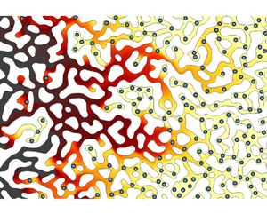
2.2. Porous medium
We consider a two-dimensional porous medium of length  $L = 167 \lambda$ and width $W = 100 \lambda$ shown in figure 1. The medium characterised by DEPs of different size connected to a network of TPs, was generated using a solid-state de-wetting process (Salvalaglio et al. Reference Salvalaglio2020; Bordoloi et al. Reference Bordoloi, Scheidweiler, Dentz, Bouabdellaoui, Abbarchi and de Anna2022). It exhibits a complex pore structure interspersed among disordered solid grains. The medium is statistically homogeneous with a porosity of $\phi = 0.39$, and a narrow pore-size distribution of mean $\lambda =30\ {\rm \mu}$m. Solutes typically diffuse and dissipate gradients within pores over time scales shorter than the time $\tau _L = L/\bar u$ needed to elute a pore volume (also referred to as the mean breakthrough time). The junctures of TPs and DEPs serve as excellent candidates to retain gradients of solute concentration, which in turn trigger DP.

Figure 1. Hyper-uniform porous structure characterised by DEPs and TPs. Computational domain with white spaces indicating solid grains (bottom).
2.3. Numerical set-up
The domain is initially saturated with solute at uniform concentration  $s_i=0.1$ mM and particles at uniform concentration $c_i=0.1$ mM. While $c_i$ may be unrealistically large, the specific value is not important here because particle concentration in the following is normalised by $c_i$. Thus, the results can be scaled to any desired (more realistic) initial value. Interactions of the particles with the solid matrix are not considered. At time $t > 0$, a sharp front of solute concentration $s_H=10$ mM is injected such that the ratio $\chi = s_i/s_H=10^{-2}$. Fluid flow is solved for no-slip boundary conditions at the fluid–solid boundary on the surface of the solid grains (see figure 1), by imposing the constant volumetric flux $U' = \phi$ at the left vertical boundary and constant pressure $p' = 0$ at the right boundary. For the solution of the solute and particle transport equations (2.3c) and (2.3d), constant flux is imposed at the inlet boundary, and zero gradient at the outlet. We use a finite element scheme to solve for the system of (2.3). For all the simulations shown here, the unstructured mesh is built using 197 723 triangular elements, the maximum size of which is $1\times 10^{-4}$ and minimum is $9\times 10^{-6}$. This corresponds to maximum and minimum resolutions of $3.33\lambda$ and $0.3\lambda$, respectively. An implicit second-order backward differentiation formulation with adaptive time stepping is used. We have checked that these results are numerically converged by performing simulations with up to 2 695 109 triangular elements with maximum and minimum element sizes of $1\times 10^{-4}$ and $6\times 10^{-6}$, respectively.
The dimensionless simulation parameters are listed in table 1. For a realistic solute diffusion coefficient of  $D_s = 10^3$ $\mathrm {\mu }$m $^2$ s $^{-1}$, this simulation scenario corresponds to $D_p = 1$ $\mathrm {\mu }$m $^2$ s $^{-1}$, $U = 25$ $\mathrm {\mu }$m s $^{-1}$, $\varGamma _p \in [-1.2,0.6] \times 10^3$ $\mathrm {\mu }$m $^2$ s $^{-1}$ and valence of the $Z:Z$ electrolyte of $Z = 1$ with a prefactor in (2.2) of $\varepsilon (k_B T)^2/\mu (Z e)^2 = 470$ $\mathrm {\mu }$m $^2$ s $^{-1}$. Note that salt diffusion coefficients are typically of the order of $10^{3}$ $\mathrm {\mu }$m $^2$ s $^{-1}$, for instance, for LiCl and NaCl, $D_s = 1600$ $\mathrm {\mu }$m $^2$ s $^{-1}$ and $D_s = 1400$ $\mathrm {\mu }$m $^2$ s $^{-1}$, respectively. The value $D_p=1$ $\mathrm {\mu }$m $^2$ s $^{-1}$ corresponds to spherical colloidal particles with diameters of approximately $500$ nm at standard room temperature ( $T = 300$ K), according to the Stokes–Einstein relation. To give a few examples, in some of the recent experiments conducted in microfluidic channels (Battat et al. Reference Battat, Ault, Shin, Khodaparast and Stone2019; Singh et al. Reference Singh, Vladisavljević, Nadal, Cottin-Bizonne, Pirat and Bolognesi2020), polystyrene colloidal particles were driven by DP arising due to gradients in monovalent solutes like NaCl and LiCl. Typical values for the diffusiophoretic mobility are $|\varGamma _p| \lessapprox 1000$ $\mathrm {\mu }$m $^2$ s $^{-1}$ (Williams et al. Reference Williams, Warren, Sear and Keddie2024).
Table 1. Domain dimensions and parameters used in the numerical simulations.

3. Results and discussion
3.1. Diffusiophoretic particle trapping/extraction
Figure 2 shows the temporal evolution of the particle concentration field without DP ( $\varGamma _p^\ast =0$), and for diffusiophoretic trapping ( $\varGamma _p^\ast <0$), and extraction ( $\varGamma _p^\ast >0$). In the absence of DP, the majority of the particles get dispersed through the TPs, leaving behind a small fraction of particles that accumulate within the DEPs, where the flow is stagnant, organised in convection rolls and described by closed streamlines (Bordoloi et al. Reference Bordoloi, Scheidweiler, Dentz, Bouabdellaoui, Abbarchi and de Anna2022). The only mechanism through which these localised particles can escape into the TPs is diffusion, the time scale of which is typically orders of magnitude larger than $\tau _L$.

Figure 2. Temporal evolution of the dimensionless particle distributions  $\log (c/c_i)$ for (a) trapping, (b) no DP and (c) extraction cases. White spaces indicate solid grains. Flow is from left to right. Note that $\tau _L/\tau _v \approx 167$ such that these plots correspond to times $0.5 \tau _L$, $1\tau _L$, $3 \tau _L$, and $10\tau _L$, approximately.
The injection of a sharp front of solute at a higher concentration results in local gradients of solute concentration that drive DP within the DEPs. For  $\varGamma _p^\ast < 0$, that is, when particles migrate from high to low solute concentrations, DP leads to the trapping of particles inside the DEPs, as shown in figure 2(a).
When  $\varGamma _p^\ast >0$, DP leads to particle mobilisation out of the DEPs because the particles move towards the higher solute concentration zones in the TPs. This is seen in the particle distributions shown in figure 2(c), where the particles within the DEPs rapidly escape the DEPs and leave the domain from the right outlet. Figure 3 shows the time evolution of the solute concentration at a point within a DEP close to the bottom of the DEP. The increase or decrease of concentration due to DP occurs on the time scale $\tau _{D_s}$, which here is smaller than $\tau _{D_p}$ by a factor of $10^3$. Thus, the action of DP on mass transfer between TPs and DEPs is limited to relatively short initial times.

Figure 3. Temporal evolution of dimensionless particle concentration ( $c/c_i$) at an arbitrary point (indicated by the arrow) within a DEP shown in the inset for $\varGamma _p^\ast <0$ (blue, trapping), $\varGamma _p^\ast =0$ (black, no DP) and $\varGamma _p^\ast >0$ (red, extraction). The particle concentrations shown in the inset are the same as in figure 2. Note that time here is non-dimensionalised by $\tau _v$, where $\tau _L/\tau _v\approx 167$.
3.2. Breakthrough curves
Figure 4(a) shows the distribution of arrival times of particles at the outlet, also known as breakthrough curves. Similar to Bordoloi et al. (Reference Bordoloi, Scheidweiler, Dentz, Bouabdellaoui, Abbarchi and de Anna2022), we observe two distinct transport regimes for all the cases. At times of the order of  $\tau _L$, particles at the outlet are produced by advection and dispersion from the TPs. For times $t \gg \tau _L$, the arrival time distribution deviates from the exponential decay predicted under the classical dispersion framework (denoted by the dotted curve in figure 4a) and displays a power law tailing. This is attributed to the particles that are initially trapped within the DEPs which can only escape the closed streamlines via diffusion, the time scale of which is typically large of the order of $\tau _{D_p} \gg \tau _v$ (here, $Pe = 1923$). For $\varGamma _p^\ast < 0$, a larger number of particles are trapped initially in the DEP, which manifests in a stronger tailing than the case without DP (indicated by black). For $\varGamma _p^\ast > 0$, particles are extracted from the DEP at initial times, and thus the tailing is weaker than for $\varGamma _p^\ast \leq 0$. Note that, albeit unphysical, extreme values of $|\varGamma _p^\ast |$ are chosen for the breakthrough curves in figure 4(a) to demonstrate the exaggerated effects of DP. The range of physically relevant values was discussed earlier in § 2.

Figure 4. (a) Arrival time distribution  $F(t)$ at the outlet for (blue circles) $\varGamma _p^*=\varGamma _p/D_s = -1.2$, (black diamonds) $0$ and (orange circles) $0.6$. The dotted grey line indicates classical prediction under the advection-dispersion framework in (3.2), where the hydrodynamic dispersion is fitted to be $D_h = 7.43$. Solid lines correspond to the travel-time model in (3.1). Note that time here is made dimensionless using $\tau _v$, where $\tau _L/\tau _v\approx 167$. (b) Effective trapped particle fraction $\alpha$ in the DEPs from the (symbols) numerical data, and (solid line) the analytical expression (3.7) for $\ell _0^\ast = 1.6/Pe_p$.
The arrival time distribution computed using numerical simulations is predicted analytically by modelling this distribution as the superposition of the residence time distributions in the TPs and DEPs (Bordoloi et al. Reference Bordoloi, Scheidweiler, Dentz, Bouabdellaoui, Abbarchi and de Anna2022)
 \begin{equation} F(t') = (1-\alpha) F_0(t')+ \alpha \int_0^\infty \text{d}\tau \frac{g(t'/\tau)}{\tau} f_D(\tau), \end{equation}
where  $\alpha$ is the effective fraction of particles in the DEPs after particle redistribution due to DP at the short initial time interval, as discussed in the previous section. The first term on the right side of (3.1) describes transport in the TP by the solution of a one-dimensional advection-dispersion equation characterised by the mean flow velocity $\bar u = U/\phi$ and a constant hydrodynamic dispersion coefficient $D'_h$. The breakthrough curve at $x' = L'$ for a uniform distribution of particles in $0< x' < \infty$ is then given by (Kreft & Zuber Reference Kreft and Zuber1978)
 \begin{equation} F_0(t') = 1 - \text{erfc}\left(\frac{L' - U't'/\phi}{\sqrt{4 D'_h t'}} \right) - \frac{D'_h \phi}{U'} \frac{\exp\left[\dfrac{(L' -U' t')^2}{4 D'_h t'} \right]}{\sqrt{4 D'_h t'}}. \end{equation}
The dimensionless hydrodynamic dispersion coefficient is obtained by fitting (3.2) to the numerical data. We find  $D'_h = 7.43$. The dimensional dispersion coefficient is given by $D_h = U \lambda D_h'/\phi$. The second term on the right side of (3.1) corresponds to the breakthrough curve of the effective fraction $\alpha$ of particles in DEPs. The function $g(t')$ is given by the Gamma distribution
 \begin{equation} g(t') = \frac{t'^{{-}2/3}\exp ({-}t')}{\varGamma (1/3)}, \end{equation}
which denotes the residence time distribution in a DEP whose characteristic diffusion time is  $\tau _\varLambda = 1$. The function $f_D(\tau )$ denotes the distribution of (dimensionless) diffusion times $\tau _\varLambda = \varLambda ^2 Pe_p$ within DEPs of (dimensionless) depth $\varLambda$, which is obtained from the distribution $f_\varLambda$ of depths through the map $\varLambda \to \varLambda ^2 Pe_p$. Equation (3.1) is used to model the numerical breakthrough curves by adjusting the effective trapped particle fraction $\alpha$ for different values of $\varGamma _p^\ast$.
As we see in figure 4(a), expression (3.1) is able to capture the early and late behaviours of the numerical breakthrough curves, but underestimates the arrival time distribution at intermediate times. This is due to the fact that expression (3.2) accounts for heterogeneity in the TPs by a constant hydrodynamic dispersion coefficient. This assumes that the characteristic advection times along TPs are much smaller than the mean arrival time at the outlet. The intermediate tailing observed here indicates that the heterogeneity of the TPs gives rise to larger advection times. While these effects can be quantified systematically in the framework of continuous time random walks (Dentz et al. Reference Dentz, Icardi and Hidalgo2018), we do not account for them in the current model because we focus here on the impact of DP on the long-time tailing of colloids, which is caused by mass transfer between TPs and DEPs. Figure 4(b) shows  $\alpha$ vs $\varGamma _p^\ast$. For $\varGamma _p^\ast < 0$ particles are trapped in the DEPs by DP as the medium is flushed. Thus, for $\varGamma _p^\ast < 0$, $\alpha$ is larger than the trapped particle fraction $\alpha _0$ for the no-DP case ( $\varGamma _p^\ast =0$). The tailing of the breakthrough, which is caused by particle retention in DEPs, is stronger than for $\varGamma _p^\ast = 0$. For $\varGamma _p>0$, particles are extracted from the DEPs when the medium is flushed. Thus, the effective trapped particle fraction is $\alpha < \alpha _0$. As a consequence, the tailing is weaker than for the no-DP scenario. The physical role of DP is to alter the effective trapped particle fraction $\alpha$ in the DEPs, and thus the tails of the particle breakthrough curves. This behaviour is correctly captured by (3.1).
3.3. Analytical model to understand how DP controls particle transport
To understand how DP controls the macroscopic fate of the suspended particles, we now estimate analytically the effective trapped particle fraction  $\alpha$. To this end, we consider a single DEP of length $\ell _p$ connected to a TP with a width $\lambda$. We provide here an outline of the derivation of the analytical model. Further details can be found in the Appendix A. Note that, for clarity, the derivation is in dimensional terms, while the final result for the effective trapped fraction $\alpha$ is again in dimensionless terms.
We assume that particle motion in the DEPs is dominated by the diffusiophoretic drift when the salt gradients are large and represent particle transport by an advection equation. This allows us, by integration, to determine the total mass  $m_{dp}$ of particles in the DEPs as a function of the particle concentration $c_0(t)$ and diffusiophoretic drift $u_0(t)$ at the interface between TPs and DEPs
 \begin{equation} m_{dp} = m_i + w \int_0^\infty {\rm d}t \,u_{0}(t) c_0(t), \end{equation}
where  $m_i$ is the initial particle mass and $w$ the width of the interface between TP and DEP. Note that $\alpha = \alpha _0 m_{dp}/m_i$, where $\alpha _0$ is the effective trapped particle fraction for the no-DP case. In order to determine the diffusiophoretic drift at the interface, we estimate the salt gradient at the interface. We find an analytical solution by using the fact that salt transport in the DEPs is dominated by diffusion. From that and the definition (2.1) of the diffusiophoretic drift, we obtain the expression
 \begin{equation} u_0(t) ={-} \frac{\varGamma_p (1 - \chi) }{\sqrt{4 {\rm \pi}D_s t}} H(\tau_{D_s} {\rm \pi}- t), \end{equation}
where  $H(t)$ denotes the Heaviside step function and $\tau _{D_s}$ is the characteristic salt diffusion time across the DEP. In order to estimate the particle concentration $c_0(t)$ at the interface, we distinguish between particle extraction ( $\varGamma _p > 0$) and particle trapping ( $\varGamma _p < 0$). In the former case, we set $c_0(t) = c_i$ equal to the resident particle concentration in the TP because the concentration of particles that are advected past the DEPs is constant. In the case of trapping ( $\varGamma _p<0$), this is different. In this case, the particle concentration $c_0(t)$ at the interface is determined by the balance of the diffusive flux of particles from the TP toward the interface, and the diffusiophoretic flux from the interface into the DEP
 \begin{equation} - D_p \frac{c_0(t) - c_i}{\ell_0} = u_{0}(t) c_0(t). \end{equation}
The characteristic gradient scale  $\ell _0$ can be estimated by equating the advective flux past the DEP and the diffusive flux toward it, which gives $\ell _0 \sim D_p/U$. Combining these relations, we obtain the following expression for $\alpha$ as a function of $\varGamma _p^\ast = \varGamma _p / D_s$:
 \begin{align} \alpha &= \alpha _0 [1 - \varGamma_p^\ast (1-\chi)] \nonumber\\ & \quad +H(-\varGamma_p^\ast) \left\{ \frac{{2 \varGamma_p^\ast}^2 (1 - \chi)^2 Pe_{p} \ell_0^\ast}{{\rm \pi} Pe_s} \ln\left[\frac{2\varGamma_p^\ast (1 - \chi) Pe_{p} \ell_0^\ast}{2\varGamma_p^\ast (1 - \chi) Pe_{p} \ell_0^\ast - {\rm \pi}Pe_s } \right] \right\}. \end{align}
The dimensionless gradient scale  $\ell _0^\ast = \ell _0/\lambda$ is inversely proportional to the particle Péclet number such that we set $\ell _0^\ast = \varSigma /Pe_p$ with $\varSigma$ a number of order one. The latter is the only fitting parameter of the derived model, which fits the data perfectly for $\varSigma = 1.6$, as shown in figure 4(b).
As mentioned above, for positive  $\varGamma _p^\ast > 0$ particles are extracted from the DEPs. In fact, by setting $\alpha = 0$ in expression (3.7), we find that particles are depleted from the DEPs for diffusiophoretic mobilities that are larger than the critical value
 \begin{equation} \varGamma_c^\ast = 1/(1 - \chi), \end{equation}
as shown in figure 4(b), where  $\varGamma _c^\ast \sim 1$. This value corresponds to the extreme case of extraction, where the particles in the DEP will be completely depleted, i.e. when $\alpha =0$. In the opposite case of negative $\varGamma _p^\ast < 0$, DP leads to the trapping of particles in the DEPs. As $\varGamma _p^\ast$ decreases toward more negative values, the fraction $\alpha$ converges toward the asymptotic value
 \begin{equation} \alpha_{\infty} = \alpha_0 \left(1 + \frac{{\rm \pi} Pe_s}{\varSigma}\right), \end{equation}
which is obtained by taking the limit of  $\varGamma _p^\ast \to \infty$. This result shows that the fraction of trapped particles cannot grow without bound. This is due to the fact that, for strongly negative diffusiophoretic mobilities, the rate at which particles are transferred to the interface between TPs and DEPs becomes smaller than the rate at which particles can be transferred into the DEPs by DP. In other words, the supply of particles to the interface is finite and does not increase as $\varGamma _p^\ast$ decreases. The analytical model describes the full dependence of $\alpha$ on $\varGamma _p^\ast$, as shown in figure 4(b) for both extraction from and trapping in DEPs, and thus seems to correctly capture the controls of DP on the macro-scale dispersion of particles.
4. Conclusions
To summarise, we investigate the effects of diffusiophoresis on particle dispersion in complex porous media. Using pore-scale simulations and analytical modelling, we have quantified the microscopic interactions between DP and flow and transport through porous media to show how this interplay impacts and governs the macroscopic fate of the colloidal particles. More precisely, we have demonstrated how DP occurring locally and microscopically with typically small time scales  $\tau _{D_s}$, impacts the macroscopic particle breakthrough curves. We show that the physical role of DP is to alter the effective trapped particle fraction within the DEPs, referred to as $\alpha$. This is quantified using a novel analytical model derived in (3.7) to give a relation between $\alpha$ and the diffusiophoretic mobility $\varGamma _p$. Despite being a localised and short-term phenomenon, DP affects the long-term distribution of the particle arrival times by reorganising the local partitioning of particles between the DEPs and TPs. Depending on the sign of $\varGamma _p$, DP can facilitate particle mobilisation out of the DEPs or it may lead to particle entrapment within. The main implication of our results is that it is possible to access regions in the complex pore space that were initially inaccessible by merely exploiting inherent salt concentration landscapes. This suggests that DP can be used as a tool for controlling particle dispersion and filtration in complex porous media.
The potential of DP to control particle migration in simple microfluidic channels and cavities has been demonstrated and well established in the literature (Shin et al. Reference Shin, Um, Sabass, Ault, Rahimi, Warren and Stone2016; Lee et al. Reference Lee, Kim, Lee and Kim2020; Singh et al. Reference Singh, Vladisavljević, Nadal, Cottin-Bizonne, Pirat and Bolognesi2020; Somasundar et al. Reference Somasundar, Qin, Shim, Bassler and Stone2023). However, despite the ubiquity of engineered and natural porous media in environmental and industrial applications, only little has been known about the impact of DP on macro-scale particle dispersion in complex disordered media. Our work is a first step towards closing this gap by shedding light on the impact of the interaction of DP, medium structure and flow heterogeneity on large-scale particle migration. Therefore, this work not only advances our fundamental understanding but also opens avenues for developing solutions to various technological problems of socio-economic relevance including groundwater remediation and microfluidics for biomedical applications, where DEPs are quite prevalent.
Lastly, it is important to note that this study considers the thin Debye layer limit, and DP that arises from monovalent salts e.g. LiCl and NaCl. In practical scenarios it is likely that the fluid composition is more complex. More investigations are required to understand DP under the influence of multivalent (Wilson et al. Reference Wilson, Shim, Yu, Gupta and Stone2020) multiple salts (Alessio et al. Reference Alessio, Shim, Mintah, Gupta and Stone2021) and for finite Debye layer (Kirby & Hasselbrink Reference Kirby and Hasselbrink2004; Shin et al. Reference Shin, Um, Sabass, Ault, Rahimi, Warren and Stone2016). In such scenarios, the diffusiophoretic mobility takes a more complex form than the one studied here. Furthermore, the present study does not consider stirring effects arising from diffusioosmosis, that is, bulk flow adjacent to the solid walls of the porous domain, which may be expected if the solid walls are themselves charged. Also, it needs to be pointed out that the model medium under consideration is two-dimensional with explicit dead-end regions. While DEPs in three-dimensional granular media and sphere packs are not likely to occur, they are an important transport-relevant medium property in many three-dimensional porous rocks (Coats & Smith Reference Coats and Smith1964; Fatt, Maleki & Upadhyay Reference Fatt, Maleki and Upadhyay1966) and aggregated media (Philip Reference Philip1968), and in general in porous materials characterised by a bi-porous structure, such as woven fabrics (Shin et al. Reference Shin, Warren and Stone2018). Thus, we expect the reported results to be relevant also for particle transport in three-dimensional porous media.
Funding
This work has received funding from European Union's Horizon 2020 research and innovation program under the Marie Skłodowska-Curie G.A. no. 895569. M.D. and L.C.F. gratefully acknowledge funding from the Spanish Ministry of Science and Innovation through the project HydroPore (PID2019-106887GB-C31 and C33). P.d.A. acknowledges the support of FET-Open project NARCISO with grant ID 828890 and of Swiss National Science Foundation G.A. 200021 172587.
Declaration of interests
The authors report no conflict of interest.
Appendix A. Detailed derivation of the analytical model
In this appendix, we elaborate on the derivation of the analytical model described in (3.7), which gives the relation between the initial particle fraction  $\alpha$ in the DEPs and the diffusiophoretic mobility $\varGamma _p$. The main rationale behind this exercise is that the only mechanism that alters the trapped fraction $\alpha$ of particles within the DEPs is the diffusiophoretic one. Using a simplified one-dimensional model, we first compute the concentration profile and, consequently, the diffusiophoretic drift. Next, a flux balance is performed at the intersection of the DEP and TP after which, an effective trapped particle fraction $\alpha$ is estimated for a given $\varGamma _p$.
The arrival time distribution computed numerically for different values of diffusiophoretic mobilities  $\varGamma _p$ is predicted using the one-dimensional statistical model in (3.1) for different effective trapped particle fractions $\alpha$ within the DEPs. This suggests a relation between $\varGamma _p$ and $\alpha$ (see figure 4).
To understand and quantify this, we construct a one-dimensional model shown in figure 5. We assume that particle transport in the DEP at short times is dominated by the diffusiophoretic drift such that
 \begin{equation} \frac{\partial c}{\partial t} + \frac{\partial}{\partial x} u_{dp} c = 0. \end{equation}
The total mass of particles in the DEP is given by
 \begin{equation} m_{dp} = w \int_0^{\ell_p} {\rm d}\kern 0.06em x \, c, \end{equation}
where  $w$ is the pore width. Since the only flux of particles toward or from the DEP is across the DEP–TP junction, the temporal variability of the mass of particles in the DEP is equal to the mass flux at $x = 0$ and controlled by DP. Spatial integration of (A1) according to (A2) gives
 \begin{equation} \frac{\partial m_{dp}}{\partial t} = w u_{dp}(x=0,t) c(x = 0,t), \end{equation}
where we set  $u_0(t) = u_{dp}(x = 0,t)$ and $c_0(t) = c(x = 0,t)$. Note that we used that there is no flux across the boundary at $x = \ell _p$. Thus, the added or extracted mass is given by
 \begin{equation} m_{dp} = m_i + w \int_0^\infty {\rm d}t \, u_{0}(t) c_0(t). \end{equation}
In the following, we first determine the diffusiophoretic drift, then we deal with the cases of extraction ( $\varGamma _p > 0$) and addition of particles ( $\varGamma _p < 0$) separately.

Figure 5. Illustration of the one-dimensional analytical model. A single DEP of length  $\ell _p$ is connected to a (vertical) TP with a width of $\lambda$. Typical solute concentration $s$ and diffusiophoretic velocity $u_{dp}$ profiles within the DEP are shown here in red and blue, respectively. At short times, the diffusiophoretic drift is strongly localised at the interface between TP and DEP.
A.1. Diffusiophoretic drift
We focus here on estimating the drift  $u_{dp}$. The Péclet number for salt ( $Pe_s=0.75$) is so low that we can assume that diffusion dominates in the DEP. Thus, to obtain the salt concentration $s$, we solve the diffusion equation
 \begin{equation} \frac{\partial s}{\partial t} - D_s \frac{\partial^2 s}{\partial x^2} = 0. \end{equation}
We consider the boundary conditions  $s = s_H$ at $x = 0$ and $\partial s / \partial x = 0$ at $x = L$. The initial condition is $s(x, t = 0) = s_i$. In Laplace space we obtain the exact solution
 \begin{equation} s^\ast(x,\sigma) = \frac{s_i}{\sigma} + \frac{(s_H - s_i)}{\sigma} \frac{\cosh[(1 - x/\ell_p) \sqrt{\sigma \tau_{D_s}}]}{\cosh(\sqrt{\sigma \tau_{D_s}})}, \end{equation}
where  $\tau _{D_s} = \ell _p^2/D_s$ and $\sigma$ is the Laplace variable. The Laplace transform is defined in Abramowitz & Stegun (Reference Abramowitz and Stegun1972).
The Laplace transform of the diffusiophoretic velocity at  $x = 0$ is then given by
 \begin{equation} u_{0}^\ast(\sigma) ={-}\varGamma_p (1 - \chi) \frac{\tanh(\sqrt{\sigma \tau_{D_s}})}{\sqrt{\sigma D_s}}, \end{equation}
where we defined  $\chi = s_i / s_H$. The integral of the drift from $t = 0$ to $\infty$ is given by
 \begin{equation} \int_0^\infty {\rm d}t \, u_{0}(t) = u_{0}^\ast(\sigma = 0) ={-} \frac{\varGamma_p (1 - \chi) \ell_p}{D_s}. \end{equation}
This expression is used directly to estimate the total mass of trapped particles for the extraction case, as argued below. For the trapping case, however, the full time dependence of  $u_{0}(t)$ is required, as can be seen from (A4). Thus, we approximate the salt concentration profile in the DEP by the solution for a semi-infinite domain
 \begin{equation} s(x,t)=s_i + (s_H-s_i)\,\text{erfc}(x/\sqrt{4D_s t}) . \end{equation}
Using this expression, the diffusiophoretic drift is given by
 \begin{equation} u_{dp}(x,t) ={-} \varGamma_p (s_H-s_i) \frac{\exp{({-}x^2/4D_s t)}}{s(x,t)\sqrt{{\rm \pi} D_s t}}. \end{equation}
The drift at  $x = 0$ then is given by
 \begin{equation} u_{0}(t) ={-} \frac{\varGamma_p (1 - \chi) }{\sqrt{{\rm \pi} D_s t}}, \end{equation}
where we used that  $s(x=0,t) = s_H$. This expression is valid for times larger than $\tau _{D_s} = \ell _p^2/D_s$, after which the salt gradient decays exponentially fast with time. Thus, the time integral (A8) over the drift can be written in terms of the approximate solution (A11) as
 \begin{equation} - \int_0^{\tau_{D_s} a} {\rm d}t \, \frac{\varGamma_p (1 - \chi) }{\sqrt{{\rm \pi} D_s t}} ={-} \sqrt{\frac{4}{{\rm \pi} a}} \frac{\varGamma_p (1 - \chi) \ell_p}{\sqrt{D_s}}. \end{equation}
In order to match the exact expression (A8), we set  $a = {\rm \pi}/4$ and use the following the approximation:
 \begin{equation} u_{0}(t) ={-} \frac{\varGamma_p (1 - \chi) }{\sqrt{4 {\rm \pi}D_s t}} H(\tau_{D_s} {\rm \pi}- t), \end{equation}
where  $H(t)$ denotes the Heaviside step function.
A.2. Extraction of particles
In the case  $\varGamma _p > 0$, particles are extracted from the DEP. The particle concentration at $x = 0$, that is, at the interface with the TP, is set equal to $c_0(t) = c_i$, the resident particle concentration. Thus, we obtain, by integration of (A3), for the added particle mass
 \begin{equation} m_{dp} = m_i + c_i w \int_0^\infty {\rm d}t \, u_{0}(t) = m_i + c_i w u_{0}^\ast(\sigma = 0) = m_i - \frac{m_i \varGamma_p (1 - \chi)}{D_s}, \end{equation}
where  $m_i = c_i w \ell _p$ is the initial particle mass and $\chi =s_i/s_H$. Note that we used expression (A8) to arrive at this result. If $\alpha _0$ is the fraction of particle mass inside the DEP without DP, then the fraction $\alpha$ of particles after DP is
 \begin{equation} \alpha = \alpha_0 \frac{m_{dp}}{m_i}. \end{equation}
Using (A14) and setting  $\ell _p = \lambda$ (since the average pore length is approximately equal to the average pore opening in the hyper-uniform porous medium considered), we obtain
 \begin{equation} \alpha = \alpha_0 [1 - \varGamma_p^\ast (1 - \chi)], \end{equation}
where  $\varGamma _p^*=\varGamma _p/D_s$ is the dimensionless form of the diffusiophoretic mobility.
A.3. Trapping of particles
In the case  $\varGamma _p < 0$, particles are trapped from the TP into the DEP. In order to determine $c_0(t)$, we consider the balance of fluxes across the interface. For $x < 0$, that is within the TP, the particle flux transverse to the flow direction is due to diffusion. For $x > 0$, that is, in the DEP the particle flux is dominated by the diffusiophoretic drift. Thus, we can write
 \begin{equation} - D_p \frac{c_0(t) - c_i}{\ell_0} = u_{0}(t) c_0(t), \end{equation}
where  $\ell _0$ is the concentration gradient scale. We assume that the particle concentration in the flow past the interface between TP and DEP is constant and equal to the initial concentration $c_i$. We estimate $\ell _0$ as the length scale at which the diffusive flux transverse to the flow direction toward the interface is of the same order as the advective flux past the interface, that is,
 \begin{equation} U c_i \sim D_p \frac{c_i}{\ell_0}. \end{equation}
From this relation, we obtain the estimate
 \begin{equation} \ell_0 \sim \frac{D_p}U = \frac{\ell_p}{Pe_p}. \end{equation}
That is, particles within the layer of thickness  $\ell _0$ are available for trapping in the DEP.
From (A17), we obtain for  $c_0(t)$
 \begin{equation} c_0(t) = \frac{c_i}{1 + \dfrac{u_{0}(t) \ell_0}{D_p}}. \end{equation}
Inserting (A20) into (A4) gives
 \begin{equation} m_{dp} = m_i + w \int_0^\infty {\rm d}t \, u_{0}(t) \frac{c_i}{1 + \dfrac{u_{0}(t) \ell_0}{D_p}}. \end{equation}
Note that, here, we use the approximation (A13) for  $u_0(t)$ to derive an analytical expression for $m_{dp}$.
Inserting expression (A13) into the right side of (A21) gives
 \begin{equation} m_{dp} = m_i - w \int_0^{\tau_{D_s} {\rm \pi}/4} {\rm d}t \, \frac{\varGamma_p (1-\chi)}{\sqrt{{\rm \pi} D_s t}} \frac{c_i}{1 - \dfrac{\varGamma_p (1-\chi) \ell_0}{\sqrt{{\rm \pi} D_s t}D_p}}. \end{equation}
We can further write
 \begin{equation} m_{dp} = m_i - w c_i \int_0^{\tau_{D_s} {\rm \pi}/4} {\rm d}t \, \frac{ \varGamma_p (1-\chi)}{\sqrt{{\rm \pi} D_s t} - \dfrac{\varGamma_p (1-\chi) \ell_0}{D_p}}. \end{equation}
Integration of the latter gives
 \begin{equation} m_{dp} = m_i - w \ell_p c_i \left\{\frac{\varGamma_p (1-\chi)}{D_s} - \frac{2 \varGamma_p^2 (1 - \chi)^2 \ell_0}{{\rm \pi} D_s D_p \ell_p} \ln\left[\frac{2 \varGamma_p (1 - \chi)}{2 \varGamma_p (1 - \chi) - {\rm \pi}D_p \ell_p / \ell_0} \right] \right\}. \end{equation}
Thus, we obtain for  $\alpha$
 \begin{equation} \alpha = \alpha _0 \left\{1 - \frac{\varGamma_p (1-\chi)}{D_s} + \frac{2 \varGamma_p^2 (1 - \chi)^2 \ell_0}{{\rm \pi} D_s D_p \ell_p} \ln\left[\frac{2 \varGamma_p (1 - \chi)}{2 \varGamma_p (1 - \chi) - {\rm \pi}D_p \ell_p / \ell_0} \right]\right\}. \end{equation}
We set  $\ell _p = \lambda$ and define the dimensionless diffusiophoretic mobility and the dimensionless diffusion layer scale as
 \begin{equation} \varGamma^\ast_p = \frac{\varGamma_p}{D_s} , \quad \ell_0^\ast = \frac{\ell_0}{\lambda} \sim 1/Pe_p. \end{equation}
Thus, we can write expression (A26) in dimensionless form as
 \begin{equation} \alpha = \alpha _0 \left\{1 - \varGamma_p^\ast (1-\chi) + \frac{{2 \varGamma_p^\ast}^2 (1 - \chi)^2 Pe_{p} \ell_0^\ast}{{\rm \pi} Pe_s } \ln\left[\frac{2 \varGamma_p^\ast (1 - \chi) Pe_{p} \ell_0^\ast}{2 \varGamma_p^\ast (1 - \chi) Pe_{p} \ell_0^\ast - {\rm \pi}Pe_s } \right] \right\} . \end{equation}


 Open access