


1. Introduction
The lift force on finite-span airplane wings produces a pair of counter-rotating trailing vortices in the wake as sketched in figure 1(a). These vortices persist for several minutes, translating to many miles behind the airplane. To avoid hazardous vortex encounters (McGowan Reference McGowan1968; Nelson Reference Nelson2004), the US Federal Aviation Administration has established instrument flight rules that impose minimum separation distances for airplanes that land at the same airport, limiting airport capacity. In the above context, the rapid destruction of wake vortices is quite desirable. The same is true for the wake vortices behind submarines and stealth airplanes. These practical needs have motivated fundamental research of the wake vortex dynamics, and good reviews of the existing work can be found in Widnall (Reference Widnall1975), Spalart (Reference Spalart1998), Gerz, Holzäpfel & Darracq (Reference Gerz, Holzäpfel and Darracq2002) and Leweke, Le Dizès & Williamson (Reference Leweke, Le Dizès and Williamson2016).

Figure 1. (a) A sketch of the counter-rotating vortices behind a finite-span airplane wing. (b) A sketch of counter-rotating vortices.
An extensively studied model problem is sketched in figure 1(b), where one neglects the effects of the ground and studies the decay or the collapse of a pair of counter-rotating vortices in a periodic domain. The vortices are assumed to be horizontal and perpendicular to the vertical direction, and, therefore, a zigzag instability (Billant Reference Billant2010; Billant et al. Reference Billant, Deloncle, Chomaz and Otheguy2010) does not play a role. The flow is controlled by the size of the vortex,  $d$, the distance between the two vortices, $b$, the strength of the two vortices, $\varGamma$, and the fluid viscosity, $\nu$. Two non-dimensional numbers can be identified, and they are the Reynolds number, $Re_\varGamma =\varGamma /\nu$, and the non-dimensional size of the vortex core, $d^*=d/b$. For most flows in the real world, the Reynolds number is high, and the size of the vortex core is much smaller than the distance between the two vortices. Hence, $d^*$ is much smaller than 1, and $Re_\varGamma$ is larger than 1 for practically relevant flows. There are three processes that are responsible for the destruction of the vortices: short-wave instability, long-wave instability or Crow instability/sinusoidal instability (Crow Reference Crow1970), and viscous diffusion. Among the three processes, viscous diffusion is the least effective – although viscous effects are important during vortex linking and turbulence bursting. A short-wave instability, as the name suggests, is an instability at a wavelength (usually) smaller than the initial distance between the two vortices and does not involve any linking of the two primary vortices (Moore & Saffman Reference Moore and Saffman1975; Tsai & Widnall Reference Tsai and Widnall1976). A short-wave instability leads to turbulence bursts within each vortex, and at practically relevant Reynolds numbers, the vortices would go through multiple cycles of short-wave instability before long-wave instability initiates (Leweke & Williamson Reference Leweke and Williamson1998; Laporte & Corjon Reference Laporte and Corjon2000) – if the vortices are not completely destroyed by the short-wave instability (McKeown et al. Reference McKeown, Ostilla-Mónico, Pumir, Brenner and Rubinstein2020). Note that when $d^* \ll 1$, the short-wave instability is very rare (Leweke et al. Reference Leweke, Le Dizès and Williamson2016). A long-wave instability (see figure 2) is an instability at a wavelength of the order of about 10 times the initial distance between the two vortices. The exact factor depending on $d^*$; see Crow (Reference Crow1970). A long-wave instability leads to vortex linking, which gives rise to vortex rings.

Figure 2. A sketch of the long-wave instability. Here  $d_0$ is the wavelength, $a$ is the amplitude, $\varTheta$ is the inclination angle and $b_0$ is the initial distance between two vortices.
Ambient turbulence and (stable) vertical thermal stratification affect the aforementioned instabilities. The strength of vertical thermal stratification can be quantified by the Froude number,  $Fr=W_0/(N b_0)$, where $N$ is the Brunt–Väisälä frequency and $W_0=\varGamma /(2{\rm \pi} b_0)$ is the induced velocity at the distance $b_0$. The strength of ambient turbulence can be quantified by the background turbulence intensity $\epsilon ^*=(\epsilon b_0)/W_0$, where $\epsilon$ is the dissipation rate. Many have studied the effects of thermal stratification and ambient turbulence. In the following, we review the relevant work on long-wave instabilities. A basic theory of the long-wave instability is given by Crow (Reference Crow1970, Reference Crow1974). Saffman (Reference Saffman1972) and Crow & Bate (Reference Crow and Bate1976) built on Crow (Reference Crow1970)'s work and accounted for thermal stratification and ambient turbulence. Their work were further refined by Greene (Reference Greene1986), Klein, Majda & Damodaran (Reference Klein, Majda and Damodaran1995), Crouch (Reference Crouch1997) and Switzer & Proctor (Reference Switzer and Proctor2002). These theories have been carefully scrutinized. Sarpkaya (Reference Sarpkaya1983) conducted experiments with three delta wings and two rectangular wings and investigated the decay of the trailing vortices in stratified and unstratified water. The author found first that thermal stratification reduces the lifespan of the trailing vortices and second that strong thermal stratification prevents vortex linking. van Jaarsveld et al. (Reference van Jaarsveld, Holten, Elsenaar, Trieling and van Heijst2011) conducted a wind tunnel experiment and measured the decay of trailing vortices in a turbulent environment. The authors observed the short-wave instability, long-wave instability and vortices breakdown after the long-wave instability. The observed behaviour is in agreement with Crow & Bate (Reference Crow and Bate1976)'s theory, but the exact mechanism after the long-wave instability was not clear. Three-dimensional numerical simulations of the flow were not reported until about 2000. Before that, numerical simulations were mostly two dimensional (Hill Reference Hill1975; Hecht, Bilanin & Hirsh Reference Hecht, Bilanin and Hirsh1981; Spalart Reference Spalart1996; Garten et al. Reference Garten, Arendt, Fritts and Werne1998; Holzäpfel & Gerz Reference Holzäpfel and Gerz1999). While two-dimensional simulations give many insights into the descent of the trailing vortices, they cannot capture the long-wave instability. Lewellen & Lewellen (Reference Lewellen and Lewellen1996) and Lewellen et al. (Reference Lewellen, Lewellen, Poole, DeCoursey, Hansen, Hostetler and Kent1998) conducted three-dimensional large eddy simulations (LES) of aircraft wakes at conditions that mimic the realistic atmosphere. The long-wave instability leads to a series of vortex rings in their LES, which agree with the photographs taken from the ground. A lot more work is put into the model problem in figure 2. The simulation results show that weak thermal stratification accelerates vortex linking, and strong thermal stratification prevents the vortex linking (Robins & Delisi Reference Robins and Delisi1998; Holzäpfel, Gerz & Baumann Reference Holzäpfel, Gerz and Baumann2001; Garten et al. Reference Garten, Werne, Fritts and Arendt2001; De Visscher, Bricteux & Winckelmans Reference De Visscher, Bricteux and Winckelmans2013; Ortiz, Donnadieu & Chomaz Reference Ortiz, Donnadieu and Chomaz2015) – although the exact Froude number that demarcates weak stratification from strong stratification is left unspecified. The results also show that weak ambient turbulence accelerates vortex linking, and strong ambient turbulence rapidly destroys the vortices (Garten et al. Reference Garten, Arendt, Fritts and Werne1998; Robins & Delisi Reference Robins and Delisi1998; Han et al. Reference Han, Lin, Schowalter, Arya and Proctor2000a).
While the long-wave instability is fairly well understood, the collapse of the residual wake structure after the first vortex linking remains poorly understood for the following reasons. Firstly, visualizing and measuring the residual wake structures is non-trivial in a lab (Sarpkaya Reference Sarpkaya1983; van Jaarsveld et al. Reference van Jaarsveld, Holten, Elsenaar, Trieling and van Heijst2011). Secondly, aside from a few direct numerical simulations (DNS) (Garten et al. Reference Garten, Werne, Fritts and Arendt2001), most simulations are LES and rely on sub-grid scale models. Thirdly, except, for example, Misaka et al. (Reference Misaka, Holzäpfel, Hennemann, Gerz, Manhart and Schwertfirm2012), most three-dimensional simulations stop shortly after long-wave instability completes.
The purpose of this work is to study the evolution of a pair of counter-rotating vortices in a stratified and turbulent environment during and, most importantly, after long-wave instability via DNS. We vary the Froude number from  $Fr=0.5$ to $\infty$ (unstratified), the ambient turbulence intensity from $\epsilon ^*=0.01$ to 1, and the Reynolds number from $Re_\varGamma =942$ to $3768$. We will show a second vortex linking in a weakly stratified environment followed by a rapid collapse of the residual vortices.
We distinguish this second vortex linking from the secondary vortex reconnections as described by van Rees, Hussain & Koumoutsakos (Reference van Rees, Hussain and Koumoutsakos2012), Yao & Hussain (Reference Yao and Hussain2020) and Hussain & Duraisamy (Reference Hussain and Duraisamy2011), which are results of high Reynolds numbers and can be observed in an unstratified environment. Specifically, the second vortex linking described here is the linking of the primary vortex ring and is a result of thermal stratification. The secondary vortex reconnections in Yao & Hussain (Reference Yao and Hussain2020) (and various other previous works) manifest as turbulence bursts within the vortex tube (as evidenced in figure 7(c) in their paper) and are not a result of thermal stratification. In fact, the phenomenon described by Yao & Hussain (Reference Yao and Hussain2020) has been found in many other studies with different initial conditions. In the following, we briefly review the literature. Direct numerical simulation studies of the reconnection process in an unstratified environment date back to Pumir & Kerr (Reference Pumir and Kerr1987), Kerr & Hussain (Reference Kerr and Hussain1989) and Shelley, Meiron & Orszag (Reference Shelley, Meiron and Orszag1993). Melander & Hussain (Reference Melander and Hussain1988, Reference Melander and Hussain1989) showed that the reconnection process has three stages, i.e. inviscid advection, bridging and threading. Saffman (Reference Saffman1990) argued that the reconnection time scales vary logarithmically with  $Re_\varGamma$. Other works on vortex reconnection can be found in Ji & Van Rees (Reference Ji and Van Rees2022), where the authors considered the bursting of a vortex tube due to the initial axial perturbation; Ostilla-Mónico et al. (Reference Ostilla-Mónico, McKeown, Brenner, Rubinstein and Pumir2021), where the authors studied the collision of two vortex tubes at an angle; Pumir & Siggia (Reference Pumir and Siggia1990), where the authors simulated two anti-parallel vortex tubes to find the collapsing solution to the three-dimensional Euler equations; and Mishra, Pumir & Ostilla-Mónico (Reference Mishra, Pumir and Ostilla-Mónico2021), where the authors considered the collision of two vortex rings. These previous studies all consider different set-ups. The reader is directed to the recent review by Yao & Hussain (Reference Yao and Hussain2022) for a comprehensive review of the literature on vortex linking/reconnection.
The rest of the paper is organized as follows. The computational set-up is summarized in § 2, and we present the results in § 3. Conclusions are given in § 4.
2. Computational details
2.1. Governing equations
The flow is governed by the following Navier–Stokes equation with the Boussinesq approximation (Nomura et al. Reference Nomura, Tsutsui, Mahoney and Rottman2006):
 $$\begin{gather} \frac{\partial u_i}{\partial x_i} = 0, \end{gather}$$
 $$\begin{gather}\frac{\partial u_i}{\partial t} + u_j\frac{\partial u_i}{\partial x_j}={-}\frac{1}{\rho_0}\frac{\partial p}{\partial x_i} + \nu \frac{\partial^2 u_i}{\partial x_j \partial x_j} + \alpha_T T g \delta_{i3}, \end{gather}$$
 $$\begin{gather}\frac{\partial T}{\partial t} + u_j\frac{\partial \left( \bar{T}+T \right)}{\partial x_j}=\kappa \frac{\partial^2 T}{\partial x_j \partial x_j}. \end{gather}$$
Equation (2.1) is the continuity, (2.2) is the momentum conservation and (2.3) is the transport equation of the temperature. Here  $u_i$ is the velocity in the $i$th Cartesian direction, $x_i$ is the $i$th Cartesian direction, $\rho _0$ is the reference density, $p$ is the deviation of the pressure from its hydrostatic value, $\nu$ is the kinematic viscosity, $\kappa$ is the thermal diffusivity, $g$ is the gravitational acceleration, $\bar {T}(z)$ is the imposed background temperature, $\partial \bar {T}/\partial t=0$, $\partial ^2\bar {T}/\partial z^2=0$, $\partial \bar {T}/\partial z = {\rm const.}$ is the constant background temperature gradient, $T$ is the temperature fluctuation, the instantaneous temperature is given by $\tilde {T}=T_0+\bar {T}(z)+T$, $T_0$ is the reference temperature, $\delta _{ij}$ is the Kronecker delta, $\alpha _T$ is the volumetric expansion coefficient and is a constant, i.e. $\alpha _T \equiv -(1/\rho _0)(\partial \tilde {\rho }/\partial \tilde {T})$. The following length and velocity scale are used for normalization:
 \begin{equation} b_0,\quad W_0. \end{equation}
Here  $b_0$ is the distance between the two vortices at $t=0$, $W_0$ is the advection velocity at a distance $b$ from the vortex core at time $t=0$ and $\varGamma _0$ is the circulation of one vortex at $t=0$. The flow is controlled by the following three non-dimensional parameters, namely, the Reynolds number $Re_{\varGamma }$, the Froude number $Fr$ and the background turbulence intensity $\epsilon ^*$. We consider two Reynolds numbers, i.e. $Re_{\varGamma,1}=942$ and $Re_{\varGamma,2}=3768$, five Froude numbers, i.e. $Fr=0.5$, 1, 2, 4 and $\infty$, and four background turbulence intensities, i.e. $\epsilon ^*=0.01$, 0.1, 0.25 and 1. We vary the Froude number and the background turbulence intensity such that thermal stratification and background turbulence are significant at one end and insignificant at the other. Specifically, background turbulence is negligible when $\epsilon ^*=0.01$ and is dominant when $\epsilon ^*=1$; the flow is unstratified when $Fr=\infty$ and strongly stratified when $Fr=0.5$. As for the Reynolds number, the results are, by and large, insensitive to the Reynolds number – at least in the range of the Reynolds numbers considered here. This is helpful because flows in the real world are at much higher Reynolds numbers.
2.2. Initial condition
The initial condition is a superposition of two flow fields, i.e. a forced homogeneous flow and two vortices. We specify the initial condition as follows. First, we compute a forced homogeneous flow at the desired Froude number in a periodic box. We follow De Visscher et al. (Reference De Visscher, Bricteux and Winckelmans2013) and force the flow at the lowest two wavenumbers, i.e.  $k_w=2{\rm \pi} /L_x$ and $k_w=4{\rm \pi} /L_x$. The forcing is adjusted until we get the $\epsilon ^*$ we want. Figure 3 shows the normalized energy spectrum of the forced homogeneous turbulence. We see the familiar $-5/3$ scaling at the low wavenumbers – although the wavenumber range within which the energy spectrum follows the $-5/3$ scaling becomes narrower as $\epsilon ^*$ decreases. This is expected: lower background turbulence requires forcing at a lower magnitude, which results in a lower Reynolds number and a narrower inertial range. Figure 4 shows contours of the $x$ vorticity and temperature at a constant $x$ location. We see more vigorous turbulence at higher $\epsilon ^*$. Specifically, we see barely any disturbance to the thermally stratified temperature fields in figure 4(e, f) for $\epsilon ^*=0.01$ and 0.10, but strong mixing of the low and high temperature fluid in figure 4(h) for $\epsilon ^*=1$. It is worth noting that we can see the oblique pattern in figure 4(h). Similar oblique patterns have been reported in the previous simulations, e.g. figure 5 in Chung & Matheou (Reference Chung and Matheou2012) and figure 18 in Agrawal & Chandy (Reference Agrawal and Chandy2021). However, we did not find an explanation for this oblique pattern and will leave this interesting phenomenon to future investigation.

Figure 3. Energy spectra of the forced homogeneous flow in a stratified environment with  $Fr = 2$ and $\epsilon ^*=0.01$, 0.10, 0.25, 1.00. The $-5/3$ law is plotted with a dashed line.

Figure 4. Contours of the  $x$ vorticity and temperature $T$ in a constant $x$ plane. The Froude number is $Fr=2$. (a–d) Vorticity in the x-direction $\omega _x$, here the contour levels are such that they encompass the maximum and minimum values in the domain; (e–h) $(T+\bar {T})/\Delta T$, where $\Delta T=L_z\,{\rm d}\bar {T}/{\rm d}z$ is the variation of the background temperature in the vertical domain. Results are shown for (a,e) $\epsilon ^*=0.01$, (b, f) $\epsilon ^*=0.10$, (c,g) $\epsilon ^*=0.25$, (d,h) $\epsilon ^*=1.00$.
Next, we compute the flow field due to the two vortices. The locations of the vortex cores are given by
 $$\begin{gather} y_1(x) = y_{1,0} - a\sin(2{\rm \pi} nx/L_x )\cos(\varTheta), \end{gather}$$
 $$\begin{gather}z_1(x) = z_{1,0} + a\sin(2{\rm \pi} nx/L_x )\sin(\varTheta), \end{gather}$$
 $$\begin{gather}y_2(x) = y_{2,0} + a\sin(2{\rm \pi} nx/L_x)\cos(\varTheta), \end{gather}$$
 $$\begin{gather}z_2(x) = z_{2,0} + a\sin(2{\rm \pi} nx/L_x)\sin(\varTheta), \end{gather}$$
where the subscripts  $1$ and 2 denote the first and second vortex, $y_{1,0}$, $z_{1,0}$, $y_{2,0}$ and $z_{2,0}$ are constants, and $y_{2,0}-y_{1,0}=b_0$, $z_{1,0}=z_{2,0}$. The second term adds perturbations to the otherwise straight vortices at the least stable wavenumber $k_w=2{\rm \pi} n/L_x=2{\rm \pi} /(8.6b_0)$ (Crow Reference Crow1970). The amplitude of the perturbation is $a=0.05b_0$, and the inclination angle is $\varTheta = 48^{\circ }$ (Garten et al. Reference Garten, Werne, Fritts and Arendt2001). The radius of the vortex core is $\sigma =0.1b_0$, within which the vorticity magnitude is a constant $\omega _0=\varGamma /({\rm \pi} \sigma ^2)$. According to the Biot–Savart law, which is only used to construct the initial field, the two vortices give rise to the following vorticity field:
 $$\begin{gather} \omega_x(x,y,z,t=0) =\omega_0 ( {\rm e}^{-\rho_1^2/\sigma^2} - {\rm e}^{-\rho_2^2/\sigma^2} ) \cos[a \cos(2{\rm \pi} nx/L_x)], \end{gather}$$
 $$\begin{gather}\omega_y(x,y,z,t=0) ={-}\omega_0 ( {\rm e}^{-\rho_1^2/\sigma^2} + {\rm e}^{-\rho_2^2/\sigma^2} ) \sin[a \cos(2{\rm \pi} nx/L_x)] \cos(\varTheta), \end{gather}$$
 $$\begin{gather}\omega_z(x,y,z,t=0) =\omega_0 ( {\rm e}^{-\rho_1^2/\sigma^2} - {\rm e}^{-\rho_2^2/\sigma^2}) \sin[a \cos(2{\rm \pi} nx/L_x)] \sin(\varTheta). \end{gather}$$
Here
 \begin{equation} \rho_i^2 = \left( y - y_i(x) \right)^2 + \left( z - z_i(x) \right)^2 \end{equation}
measures the distance from a generic location  $(x, y, z)$ to the $i$th vortex. Figure 5 is a visualization of the two vortices. The resulting velocity field can be obtained by solving the following Laplace equation:
 \begin{equation} \nabla^2 \boldsymbol{u} ={-} \boldsymbol{\nabla} \times \boldsymbol{\omega}. \end{equation}
Figure 5. A visualization of the two vortices. The lines are stream lines at a constant  $x$ location through the mid-plane of the vortices.
The initial flow field is the superposition of the forced homogeneous turbulence and the two vortices. This way of obtaining the initial flow is similar to De Visscher et al. (Reference De Visscher, Bricteux and Winckelmans2013). The two velocity fields are both divergence free, so it does not lead to any numerical difficulty, but whether the initial field is ‘physical’ is a question worth further investigation. Figure 6 shows the isosurfaces of  $Q^*=1$ of the initial vorticity at the condition $Re=942$, $Fr=2$ and $\epsilon ^*=0.01, 1.00$, where $Q^*$ is defined as
 \begin{equation} Q^* = \frac{1}{2}(\omega_{ij}^*\omega_{ij}^* - S_{ij}^*S_{ij}^*),\quad \omega_{ij}^* = \frac{1}{2}\left(\frac{\partial u_{i}^*}{\partial x_j} - \frac{\partial u_{j}^*}{\partial x_i}\right),\quad S_{ij}^* = \frac{1}{2}\left(\frac{\partial u_{i}^*}{\partial x_j} + \frac{\partial u_{j}^*}{\partial x_i}\right), \end{equation}
and  $u_{i}^* \equiv u_i/\max (\sqrt {u_k^2})$ is the normalized velocity. The background turbulence level is low in figure 6(a), and the only visible vortical structures are the two counter-rotating vortices. On the other hand, in figure 6(b) the background turbulence level is high, and we see a lot more vortical structures than the two counter-rotating vortices.

Figure 6. The  $Q$ isosurfaces, $Q^*=1$, of the initial flow fields at (a) $\epsilon ^{\star }=0.01$ and (b) $\epsilon ^{\star }=1.00$. The isosurfaces are coloured by the $(\tilde {T}+\bar {T})/\Delta T$. The Froude number is $Fr=2$ and the Reynolds number is $Re=942$.
2.3. Further details
Twenty-one DNS are conducted. The details of the DNS are tabulated in table 1. The nomenclature of the cases is as follows:  ${\rm Fr}[Fr]{\rm E}[\epsilon ^*]{\rm Re}[{\rm L}/{\rm M}]$, where $Fr$ is 0.5, 1, 2, or 4, $\epsilon ^*$ is 0.01, 0.10, 0.25 and 1, L and M stand for low and moderate. There are four groups of DNS. In the first group, we vary the Froude number whilst keeping the background turbulence negligible. The purpose is to study the effects of thermal stratification. In the second group, we vary the background turbulence intensity whilst keeping thermal stratification negligible. The purpose is to study the effects of background turbulence. In the third group, we vary the turbulence intensity whilst keeping $Fr=2$. The purpose is to study the effects of both the background turbulence and thermal stratification. Last, in the fourth group, we vary the Reynolds number. The purpose is to show that our results are insensitive to the Reynolds number.
Table 1. Direct numerical simulation details.

The computational domain is a periodic box. Except for Fr2.0E0.01ReM, for which the domain size is  $L_x\times L_y\times L_z=8.6b_0\times 12.9b_0\times 8.6 b_0$, we employ a domain of size $L_x\times L_y\times L_z=8.6b_0\times 8.6 b_0\times 8.6 b_0$. The grid spacing is uniform in all three directions, and the resolution is slightly finer than that in Garten et al. (Reference Garten, Werne, Fritts and Arendt2001). We ensure that the grid is sufficiently fine for the high $\epsilon ^*$ cases and apply that grid to the low $\epsilon ^*$ cases. Specifically, the grid resolution is $\varDelta /\eta \leqslant 0.85$ in all DNS, where $\eta$ is the Kolmogorov length scale. The time step size is such that ${\rm CFL}=0.6$.
The in-house finite-difference code AFiD is employed for the DNS. The code is second order in space and uses the third-order Runge–Kutta scheme in time.
Further details of the numerics can be found in Ostilla-Monico et al. (Reference Ostilla-Monico, Yang, van der Poel, Lohse and Verzicco2015), van der Poel et al. (Reference van der Poel, Ostilla-Mónico, Donners and Verzicco2015) and Kim & Moin (Reference Kim and Moin1985). The code has been extensively used for stratified flows (Yang et al. Reference Yang, Van Der Poel, Ostilla-Mónico, Sun, Verzicco, Grossmann and Lohse2015, Reference Yang, Chen, Verzicco and Lohse2020; Du, Zhang & Yang Reference Du, Zhang and Yang2021; Li & Yang Reference Li and Yang2021), and we present a validation in Appendix A.
3. Result
3.1. Basic phenomenology
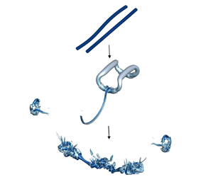
Figure 7 visualizes the evolution of the vortex pair in case Fr2.0E0.01ReM. First, the two vortices get close to each other as a result of the Crow instability. Meanwhile, they move downward as a result of induced velocity. This is shown in figure 7(a). The dissipation is about uniform in each vortex until the two vortex link, which happens at  $t^*=3$, where $t^*$ is normalized time and defined as
 \begin{equation} t^* \equiv tW_0/b_0. \end{equation}
This is the first vortex linking, and it gives rise to a vortex ring. Large dissipation is found at the location where the two vortices link, as shown in figure 7(b). The first vortex linking marks the completion of sinusoidal instability. This process is very well understood (Crow Reference Crow1970), and we leave the discussion brief. The focus of this study is the decay of the residual vorticity after the first vortex linking, which is still poorly understood.

Figure 7. Isosurface of  $Q^*=1$ at $t^*=1$, 3, 4, 5, 5.5, 6, 6.5 and 7.0 for case Fr2.0E0.01ReM. The isosurfaces are coloured by viscous dissipation. Light blue indicates low dissipation, and dark blue indicates high dissipation.
After the first vortex linking, the vertical position of the two vortices do not change significantly until the second vortex linking at  $t^*=5.5$. Between the first and second vortex linking, the size of the vortex ring collapse in the longitudinal ( $y$) direction. Specifically, among the four ends of the vortex ring, the distance between E1 and its opposite end decreases, whereas the distance between E2 and its opposite end increases, as shown in figure 7(c). This process continues, leading to two wrapped semicircle-shaped vortices in figure 7(d), followed by the second vortex linking at two locations in figure 7(e). The second vortex linking gives rise to two small vortex rings and two line vortices. The evolution of these residual vortices is shown in figure 7( f,g,h). The two small vortex rings travel left and right and leave. The two line vortices collide, leading to rapid vortex decay. In the process, we see a few weak vortex jets, which quickly dissipate. We also see turbulence bursts, which lead to the demise of the residual vortices.
To quantify the physics that is responsible for the decay of the vortices, we turn to the following kinetic energy equation:
 \begin{equation} \frac{\partial k}{\partial t} + \frac{\partial \left( u_i k \right) }{\partial x_i} ={-}\frac{1}{\rho_0}\frac{\partial \left( u_i p \right)}{\partial x_i} + \nu \frac{\partial^2k}{\partial x_i^2} - \epsilon + P_g.\end{equation}
Here the kinetic energy  $k$ is
 \begin{equation} k \equiv \frac{u_iu_i}{2}, \end{equation}
the dissipation term  $\epsilon$ is
 \begin{equation} \epsilon \equiv \nu \frac{\partial u_i}{\partial x_j} \frac{\partial u_i}{\partial x_j} \end{equation}
and the gravitational term  $P_g$ is
 \begin{equation} P_g \equiv \alpha_TTgu_3. \end{equation}
The gravitational term represents the exchange between the gravitational potential energy and kinetic energy. The dissipation term  $\epsilon$ destroys kinetic energy. Figure 8 shows the domain integrated $k$ and $\epsilon$ as a function of time. We see three distinct stages in figure 8(a): the flow loses energy quickly from $t^*=0$ to $t^*=2.6$, i.e. before the first vortex linking, barely loses any kinetic energy from $t^*=2.6$ to $t^*=5.4$, i.e. between the first and the second vortex linking, and quickly loses energy beyond $t^*=5.4$, i.e. after the second vortex linking and during the bursts. Figure 8(b) shows a similar trend: the dissipation rate dips between $t^*=2.6$ and $t^*=5.4$, i.e. between the first and the second vortex linking.

Figure 8. The volume integrated (a) kinetic energy  $\left \langle k\right \rangle$ and (b) dissipation term $\left \langle \epsilon \right \rangle$ as a function of the non-dimensional time $t^*$. Here, $k_0$ and $\epsilon _0$ are the kinetic energy and viscous dissipation at $t^*=0$.
Tools like  $Q$ isosurfaces and time histories of volume integrated kinetic energy and viscous dissipation have been extensively used in previous studies (Han et al. Reference Han, Lin, Schowalter, Arya and Proctor2000b; Moet et al. Reference Moet, Darracq, Laporte and Corjon2000; Holzäpfel et al. Reference Holzäpfel, Hofbauer, Darracq, Moet, Garnier and Gago2003; Nomura et al. Reference Nomura, Tsutsui, Mahoney and Rottman2006; Misaka et al. Reference Misaka, Holzäpfel, Hennemann, Gerz, Manhart and Schwertfirm2012). The $Q$ isosurfaces contain spatial information, but they lack temporal information. Time histories of volume integrated kinetic energy and viscous dissipation have temporal information, but they lack spatial information. In a lot of previous work (Garten et al. Reference Garten, Werne, Fritts and Arendt2001; De Visscher et al. Reference De Visscher, Bricteux and Winckelmans2013), $Q$ isosurfaces and time histories of volume integrated kinetic energy and viscous dissipation are shown together to complement each other. However, it would be rather cumbersome to show $Q$ isosurfaces and time histories of $k$ and $\epsilon$ for all DNS cases. We need a tool that contains both temporal information and spatial information. In search of such a tool, we find that the transverse ( $y$ and $z$ directions) integrated turbulent kinetic energy and viscous dissipation, i.e. $\bar {k}$ and $\bar {\epsilon }$, are good candidates. Figure 9 shows $\bar {k}$ and ${\bar {\epsilon }'}$ as a function of time, where
 \begin{equation} {\bar{\epsilon}'}=\frac{\bar{\epsilon}-\left\langle\epsilon\right\rangle}{{\rm STD}({\bar{\epsilon}-\left\langle\epsilon\right\rangle})}, \end{equation}
and  ${\rm STD}({\cdot })$ is the standard deviation of the variable in the parentheses. We see first and second vortex linking at $x/L_x=0.75$, $t^*=2.6$ and $x/L_x=0.25$, $t^*=5.4$, as well as turbulence bursts. We also see the rapid decay of the kinetic energy and the surge of viscous dissipation after the second vortex linking. Note that $\bar {k}$ and $\bar {\epsilon }'$ carry similar information. In the following subsections we will use the transverse averaged viscous dissipation and only show $Q$ isosurfaces and time histories of volume-averaged kinetic energy and dissipation rate when necessary.

Figure 9. (a) Contour of the transverse averaged kinetic energy  $\bar {k}$ as a function of the $x$ coordinate and time. (b) Same as (a) but for $\bar {\epsilon }'$.
3.2. The second vortex linking
We observe a second vortex linking followed by turbulence bursts and the rapid decay of the residual vortices. This directly contradicts the findings in Misaka et al. (Reference Misaka, Holzäpfel, Hennemann, Gerz, Manhart and Schwertfirm2012), where the residual vortices after the first vortex linking are found to persist for a long time. In this subsection we will explain this difference.
Misaka et al. (Reference Misaka, Holzäpfel, Hennemann, Gerz, Manhart and Schwertfirm2012) and this work differ in the following. Firstly, Misaka et al. (Reference Misaka, Holzäpfel, Hennemann, Gerz, Manhart and Schwertfirm2012) is an LES study, and the authors considered a higher Reynolds number. Secondly, Misaka et al. (Reference Misaka, Holzäpfel, Hennemann, Gerz, Manhart and Schwertfirm2012) considered vortex evolution in an unstratified environment. It is critical that we understand what is responsible for the long life span of the residual vortices in Misaka et al. (Reference Misaka, Holzäpfel, Hennemann, Gerz, Manhart and Schwertfirm2012). Note that we do not doubt the reliability of LES results from Misaka et al. (Reference Misaka, Holzäpfel, Hennemann, Gerz, Manhart and Schwertfirm2012). In fact, a similar long-living vortex ring is reported by other researchers, e.g. Leweke & Williamson (Reference Leweke and Williamson2011). Our unstratified case, i.e. FrInfE0.01ReL, also shows a long-living vortex ring, as demonstrated in figure 11, Thus, we think it is hard to argue that LES is responsible for the difference in life span.
Figure 10(a) shows  $\bar {\epsilon }'$ in case Fr2.0E0.01ReL. Case Fr2.0E0.01ReL is at the same condition as case Fr2.0E0.01ReM except that case Fr2.0E0.01ReL is at a lower Reynolds number. We see the first vortex linking at $x/L_x=0.75$, $t^*=3.5$, the second vortex linking at $x/L_x=0.25$, $t^*=7$, and the subsequent turbulence bursts; this is similar to figure 9(b). Figure 10(b,c) shows the $Q$ isosurfaces at $t^*=7$ and 9. We see turbulence bursts as in figure 7(h). However, because the flow is at a lower Reynolds number than Fr2.0E0.01ReM, we see only one bulb of eddies and fewer structures in figure 10 than in figure 7(h). Hence, the Reynolds number cannot explain the difference between Misaka et al. (Reference Misaka, Holzäpfel, Hennemann, Gerz, Manhart and Schwertfirm2012) and the present work. Figure 11 shows the transverse averaged dissipation rate $\bar {\epsilon }'$ in case FrInfE0.01ReL. Case FrInfE0.01ReL is at the same condition as Fr2.0E0.01ReL except that FrInfE0.01ReL is unstratified. We see the first vortex linking at $t^*=4$. Figures 11(b,c,d) show the $Q$ isosurfaces at $t^*=10$, 20 and 30. We do not see second vortex linking nor turbulence bursts. Instead, the vortex ring oscillates and persists for a long time. Hence, we conclude that the unstratified environment is responsible for the long life span of the residual vortices in Misaka et al. (Reference Misaka, Holzäpfel, Hennemann, Gerz, Manhart and Schwertfirm2012). In other words, the stratified environment causes the second vortex linking.

Figure 10. (a) Same as figure 9(b) but for case Fr2.0E0.01ReL. Isosurface of  $Q^*=0.6$ at (b) $t^* = 7$ and (c) $t^* = 9$.

Figure 11. (a) Same as figure 9(b) but for case FrInfE0.01ReL. Isosurface of  $Q^*=0.6$ at (b) $t^* = 10$, (c) $t^* = 20$ and (d) $t^* = 30$.
Next, we interrogate the DNS for the flow structures that are responsible for the second vortex linking in a stratified environment. Figure 12(a) shows the contour of the  $y$-direction vorticity $\omega _y$ at $y=0.5(L_y+b_0)$, $t^* = 5$ in Fr2.0E0.01ReM, which is slightly off centre and at a time before the second vortex linking. The centres of the primary vortices are at $(x,z)=(0.17L_x,0.44L_z)$ and $(x,z)=(0.33L_x,0.44L_z)$. The primary vortices induce secondary vortices, as indicated in figure 12(a). We may roughly divide the secondary vortices into the upper part and the lower part, whose $z$ coordinates are above and below that of the primary vortices. We see that the upper part is stronger than the lower part. Consequently, the secondary vortices induce a velocity that pushes the left primary vortex to the right and the right primary vortex to the left. This eventually leads to the second vortex linking, as we see in figure 7(e–f). This is consistent with the previous studies, where the distance between two counter-rotating vortices decreases in a stratified environment (Saffman Reference Saffman1972; Spalart Reference Spalart1996; Garten et al. Reference Garten, Arendt, Fritts and Werne1998; Ortiz et al. Reference Ortiz, Donnadieu and Chomaz2015). Figure 12(b) shows $y$ vortices in Fr2.0E0.01ReL before the second vortex linking. We see, again, the secondary vortices, which have a comparably stronger upper part and a comparably weaker lower part. Lastly, figure 12(c) shows the contours of the $y$ vortices in FrInfE0.01ReL after the first vortex linking. This case does not give rise to a second vortex linking, and in figure 12(c) we see no secondary vortices. In all, we conclude that the second vortex linking is a consequence of the secondary vortices, which are due to flow stratification.

Figure 12. Contours of the  $y$-direction vorticity $\omega _y$ on $y=0.5(L_y+b_0)$ plane for (a) case Fr2.0E0.01ReM at $t^*=5$, (b) case Fr2.0E0.01ReL at $t^*=6$ and (c) case FrInfE0.01ReL at $t^*=7$. To show secondary vortices clearly, the contours are respectively normalized by (a) $0.1\omega _{y,m}$, (b) $0.2\omega _{y,m}$ and (c) $0.2\omega _{y,m}$. Here, $\omega _{y,m}$ is the maximum $y$-direction vorticity on each plane.
The generation of the secondary vortices can be attributed to the  $P_g$ term in (3.2). In figure 13 we examine the behaviour of the term $P_g$. Figure 13(a) shows the evolution of the volume integrated $P_g$ in the Fr2.0E0.01ReL case. It first decreases, then increases and finally decreases again. Figure 13(b,c) shows the contours of $P_g$ before the first and second vortex linking at a constant $x$. We see that the term is negative between the two primary vortices (the locations of the two primary vortices are indicated using two arrows) and positive on the outer sides of the vortices, which subsequently leads to the secondary vortices (as shown in figure 12a).

Figure 13. (a) The volume integrated gravitational term  $\left \langle P_g \right \rangle$ as a function of $t^*$, where $\left \langle \epsilon _0 \right \rangle$ is the volume integrated initial dissipation. (b) Contour of $P_g$ at $t^* = 3,x = 0.75L_x$. (c) Contour of $P_g$ at $t^* = 6,y = 0.5(L_y+b_0)$ in case Fr2.0E0.01ReL. Here $P_{g,m}$ is the maximum value of $P_g$ in the plane, and arrows indicate the location of the primary vortices.
In the next few subsections we discuss the impacts of stratification and background turbulence. Again, the discussion will focus on the evolution of the vortices after the first vortex linking (at large  $t^*$).
3.3. Thermal stratification and background turbulence
First, we vary the Froude number from 0.5 to  $\infty$ whilst keeping the Reynolds number $Re_\varGamma =942$ and $\epsilon ^*=0.01$ constant. The background turbulence is negligibly weak and insignificant. As we will show, the flow is strongly stratified when $Fr\leqslant 0.7$, weakly stratified when $Fr>0.7$, and unstratified conditions when $Fr=\infty$.
Figure 14 shows the transverse averaged dissipation  $\bar {\epsilon }'$ as a function of both $x$ and $t^*$ for $Fr=0.5$, 1 and 4. The $Fr=2$ result is shown in figure 10(a) and the $Fr=\infty$ result is shown in figure 11(a). The $Fr=1$, 2, 4 results are qualitatively similar. The first vortex linking occurs at $t^*=3.7$, 3.5, 3.0 and 2.5 for $Fr=\infty$, 4, 2 and 1, respectively. The second vortex linking occurs at $t^*=8.3$, 6.5 and 5.2 for $Fr=$4, 2 and 1, respectively, and the time it takes for the vortices to link a second time decreases as the Froude number decreases (as stratification becomes stronger). There is no second vortex linking when $Fr=\infty$. The $Fr=0.5$ result is qualitatively different from the rest, and we see no vortex linking at all. These results are consistent with those in Garten et al. (Reference Garten, Arendt, Fritts and Werne1998, Reference Garten, Werne, Fritts and Arendt2001), and Sarpkaya (Reference Sarpkaya1983): thermal stratification accelerates sinusoidal instability until strong stratification prevents sinusoidal instability completely. These results are also consistent with the results in § 3.1: a second vortex linking occurs in a weakly stratified environment.

Figure 14. Transverse averaged dissipation  $\bar {\epsilon }'$ in case (a) Fr0.5E0.01ReL, (b) Fr1.0E0.01ReL, (c) Fr4.0E0.01ReL.
In case Fr0.5E0.01ReL vortex linking is prevented completely. To get some insights into the flow dynamics, figure 15 shows the contour of the  $x$-direction vorticity $\omega _x$. We see gravitational waves in (b–d). The vortex pair gives rise to secondary vortices, which, in turn, give rise to tertiary vortices and quaternary vortices. This process would continue indefinitely until the gravitational waves drain the kinetic energy in the vortex pair.

Figure 15. Contour of normalized  $x$-direction vorticity $\omega _x/\omega _{x,m}$ at $x = 0.5L_x,$ (a) $t^* = 1$ , (b) $t^* = 2$, (c) $t^* = 3$, (d) $t^* = 4.$ Here $\omega _{x,m}$ is the maximum value of $\omega _{x}$.
Quantitatively speaking, the energy loss due to gravitational waves can be obtained by computing the energy flux at the surface of a control volume that encompasses the primary vortices. We define the control volume as in figure 15(d). It is a rectangular box and encompasses  $y/L_y\in [0.2,0.8],z/L_z\in [0.3,0.7]$. The flux due to pressure waves is given by
 \begin{equation} F_p \equiv \oint_V \frac{p\boldsymbol{u}}{\rho_0}\boldsymbol{\cdot} {\boldsymbol{n}}\,{\rm d}S, \end{equation}
where  ${\boldsymbol {n}}$ is the normal vector pointing from the inside of the control volume to the outside. Thus, positive $F_p$ corresponds to the energy loss. We normalize $F_p^*$ with $W_0$ and $b_0$ like other quantities. Figure 16 shows $F_p^*$ as a function of $t^*$. We see that $F_p^*$ is positive shortly after the initial transient period, and, thus, the primary vortices keep losing energy to internal gravitational waves.

Figure 16. The flux of the pressure term  $F_p^*$ on the control volume as the function of $t^*$.
A question we could ask is how stratification generates secondary vortices in a strongly stratified environment. The governing equation for vorticity is
 \begin{equation} \frac{\partial \omega_i}{\partial t} + u_j\frac{\partial \omega_i}{\partial x_j} - \omega_j\frac{\partial u_i}{\partial x_j} = \nu \frac{\partial^2 \omega_i}{\partial x_j^2} + \alpha_Tg\left(\delta_{1i}\frac{\partial T}{\partial y} - \delta_{2i}\frac{\partial T}{\partial x}\right), \end{equation}
where the last term shows that stratification generates vorticity. Figure 17 shows the contour of the normalized temperature at the same  $x$ location and time $t^*$ as figure 15(a). The primary vortex pair brings the lighter fluid among the heavier fluid. In these regions, $\partial T/\partial y \ne 0$, and vortices are generated as a result. This process, of course, will not happen in unstratified flows.

Figure 17. Contour of the normalized temperature  $(T+\bar {T})/\Delta T$ at the same $x/L_x$ and $t^*$ as figure 15(a).
Having discussed the effects of thermal stratification, next, we vary the background turbulence level from  $\epsilon ^*=0.01$ to 1.0 whilst keeping the Froude number at $Fr=\infty$ and the Reynolds number at $Re_\varGamma =942$. The background turbulence is weak when $\epsilon ^*=0.01$ and 0.1 and strong when $\epsilon ^*=0.25$ and 1. Recall that the vortex ring, which directly results from the first vortex linking, persists for a long time in the absence of background turbulence. In the following, we examine the impact of background turbulence on the vortex ring.
Figure 18 shows the time histories of the volume integrated kinetic energy and viscous dissipation. We normalize the kinetic energy and the viscous dissipation by their values at  $t^*=0$ in case FrInfE0.01ReL. The background turbulence contributes to the kinetic energy and the dissipation: at $t^*=0$, the normalized kinetic energy is 22.5, 2.06, 1.14 in cases FrInfE0.10ReL, FrInfE0.25ReL and FrInfE1.00ReL, and the normalized dissipation is 11, 1.114, 1.007. When the background turbulence is strong, the vortex pair is a lesser part of the flow. It should follow that the flow is less controlled by the vortex dynamics in the presence of strong background turbulence. This is not immediately clear from figure 18: in all cases, the kinetic energy and the dissipation decay as a function of time. To get some insights into the flow dynamics, we examine the transverse averaged viscous dissipation.

Figure 18. The volume integrated (a) kinetic energy and (b) viscous dissipation as a function of time, where  $\left \langle k_0 \right \rangle$ and $\left \langle \epsilon _0 \right \rangle$ is the initial volume integrated value in the FrInfE0.01ReL case.
Figure 19 shows the transverse averaged dissipation  $\bar {\epsilon }'$. The FrInfE0.01ReL result is shown in figure 11(a). Background turbulence disturbs the flow. The $\epsilon ^*=0.10$ and 0.25 results in (a,b) look qualitatively similar to the $\epsilon ^*=0.01$ result in figure 11(a). We see the first vortex linking at $t^*=3.3$, $x/L_x=0.57$ and $t^*=1.5$, $x/L_x=0.55$, respectively, but no second vortex linking. Nonetheless, the vortex ring (a result of the first vortex linking) does not necessarily persist for a long time. In case FrInfE1.00ReL the background turbulence is so strong that it tore the vortex pair quickly, as we can see in (c). To see what is happening in the flow when there is strong background turbulence, we visualize the vortices in case FrInfE1.00ReL in figure 20. We see that the background turbulence quickly dissipates the vortex pair, and at $t^*=2$ we can no longer find the vortex pair.

Figure 19. Transverse integrated dissipation  $\bar {\epsilon }'$ in case (a) FrInfE0.10ReL, (b) FrInfE0.25ReL and (c) FrInfE1.00ReL.

Figure 20. Isosurface of  $Q^*=5$ for the FrInfE1.00ReL case at $t^* = 2$.
So far, we varied the Froude number in a flow where there is essentially no background turbulence. We also varied the background turbulence level in a flow with no stratification. Now, we consider a flow with both thermal stratification and background turbulence. Specifically, we vary the background turbulence intensity from  $\epsilon ^*=0.01$ to 1.0 whilst keeping $Fr=2.0$ and $Re_\varGamma =942$. The objective is to see if there is any nonlinear interplay between thermal stratification and background turbulence.
Figure 21 shows the transverse averaged dissipation  $\bar {\epsilon }'$ in cases Fr2.0E0.10ReL, Fr2.0E0.25ReL and Fr2.0E1.00ReL. The Fr2.0E0.01ReL results are shown in figure 10. When the background turbulence is at a low level, i.e. $\epsilon ^*=0.10$, there is a second vortex linking and subsequent turbulence bursts. However, when the background turbulence is at a high level, i.e. $\epsilon ^*=0.25$, 1.00, the two vortices rapidly dissipate, and there is no second vortex linking. In all, we do not see any apparent nonlinear interplay between thermal stratification and background turbulence: thermal stratification plays the dominant role when the background turbulence level is low, and background turbulence plays the dominant role when it is strong.

Figure 21. Transverse averaged dissipation  $\bar {\epsilon }'$ in case (a) Fr2.0E0.10ReL, (b) Fr2.0E0.25ReL and (c) Fr2.0E1.00ReL.
3.4. Critical Froude number
The second vortex linking can be observed in a weakly stratified environment but not in a strongly stratified and unstratified environment. Therefore, there must be two critical Froude numbers  $Fr_{c1}$ and $Fr_{c2}$, and the second vortex linking can only be observed between $Fr_{c1}$ and $Fr_{c2}$. In this subsection we try to find these two critical Froude numbers.
Figure 22 shows the contours of  $\bar {\epsilon }'$ for Fr0.6E0.01ReL, Fr0.7E0.01ReL, Fr0.8E0.01ReL and Fr0.9E0.01ReL. Figure 23 shows the $Q$ isosurfaces for Fr0.6E0.01ReL, Fr0.7E0.01ReL, Fr0.8E0.01ReL at the time we expect to see the vortex linkings. Long-wave instability leads to the first vortex linking in all cases, but the second vortex linking is found in Fr0.8E0.01ReL and Fr0.9E0.01ReL only. Hence, $Fr_{c1}$ is between 0.7 and 0.8. Figure 24 shows the contours of $\bar {\epsilon }'$ for Fr4.0E0.01ReL, Fr6.0E0.01ReL and Fr8.0E0.01ReL. We see the second vortex linking in Fr4.0E0.01ReL and Fr6.0E0.01ReL but not in Fr8.0E0.01ReL ( $\bar {\epsilon }'$ does not intensify as in the other two cases). Hence, $Fr_{c2}$ is between 6.0 and 8.0. Further pinpointing of the two critical Froude numbers (to two significant digits) is left for future investigation.

Figure 22. Contour of  $\bar {\epsilon }'$ as a function of the $x$ coordinate and the time for case (a) Fr0.6E0.01ReL, (b) Fr0.7E0.01ReL, (c) Fr0.8E0.01ReL, (d) Fr0.9E0.01ReL.

Figure 23. Isosurface of  $Q^*$ for case (a,b) Fr0.6E0.01ReL, (c,d) Fr0.7E0.01ReL, (e, f) Fr0.8E0.01ReL. The $Q^*$ isosurfaces at the time of (a,c,e) the first vortex linking, (b,d) turbulence bursting and ( f) the second vortex linking.

Figure 24. Same as figure 22, but for case (a) Fr4.0E0.01ReL, (b) Fr6.0E0.01ReL, (c) Fr8.0E0.01ReL. Here  $\bar {\epsilon }'$ intensifies when the second vortex linking occurs, which happens in (a,b) but not in (c).
Next, we discuss how the Reynolds number may affect the values of the two critical Froude numbers. Comparing Fr2.0E0.01ReL and Fr2.0E0.01ReM, we notice that the second vortex linking leads to vortex bursts. Since the violent bursts become more violent as the Reynolds number increases, suggesting that it is more likely to observe the second vortex linking at high Reynolds numbers. Hence,  $Fr_{c1}$ and $Fr_{c2}$ should decrease and increase slightly as the Reynolds number increases – until the Reynolds number is sufficiently high and these events no longer depend on the Reynolds number. Likewise, comparing Fr2.0E0.01ReL and Fr2.0E0.10ReL, we note that strong background turbulence distorts the vortices and makes vortex linking (first and second) more difficult. Hence, $Fr_{c1}$ and $Fr_{c2}$ should increase and decrease slightly as the background turbulence increases – until background turbulence completely prevents vortex linking.
4. Conclusions
We conduct DNS to study the evolution of a vortex pair in a stratified and turbulent environment. Direct numerical simulations continue after the long-wave instability completes, and we study the decay of the residual vortices.
In addition to conventional tools like the time histories of the volume integrated dissipation rate and kinetic energy, which contain only temporal information but no spatial information, and  $Q$ isosurfaces, which contain only spatial information but no temporal information, the transverse averaged dissipation rate is employed. The transverse averaged dissipation rate contains both temporal and spatial information, and one can easily identify dynamically important events from the plot.
The main finding of the paper is the second vortex linking, which has not been reported before. It occurs after the first vortex linking, i.e. after the Crow instability completes, in a weakly stratified environment when the background turbulence is not very strong. The second vortex linking is followed by turbulence bursts and the rapid decay of residual vortices, the latter of which is responsible for the short life span of the vortex pair. The finding challenges the conventional view that the residual vortices have a long life span, which is only true if the environment is not stratified.
The decay of the residual vortices after the first vortex linking is, in general, poorly understood. In addition to the second vortex linking, our findings include the following. The vortex ring persists for a long time in an unstratified environment in the absence of background turbulence. In a strongly stratified environment, vortex linking is completely prevented, and the vortex pair loses energy to gravitational waves. Background turbulence distorts the vortex ring and helps to dissipate the large eddies in the flow. When the background turbulence is strong, no vortex linking can be observed, and the vortex pair is rapidly torn apart by the background turbulence. Finally, there is no apparent nonlinear interplay between thermal stratification and background turbulence when both are present.
Figure 25 summarizes our data in the  $Fr$–
$Fr$– $\epsilon ^*$ phase space: there exists a regime with no vortex linking (region 1), a regime with the first but not the second vortex linking (region 2) and a regime with both vortex linking events (region 3). More DNS are certainly needed to accurately determine the boundary of these regimes, which is left for future investigation.

Figure 25. Parameter space. Three regimes can be identified: a regime with no vortex linking (region 1), a regime with the first but not the second vortex linking (region 2), and a regime with both vortex linking events (region 3). The case with no vortex linking is coloured black; the case with the first but not the second vortex linking is coloured red; and the case with both vortex linking events is coloured blue.
We end the paper with a discussion on the practical relevance of this study. The Froude number range investigated in this paper covers the typical flight conditions (Lewellen & Lewellen Reference Lewellen and Lewellen1996). The DNS Reynolds number, however, is much lower than the flight Reynolds number, which is  $O(10^7)$ per our definition. Direct numerical simulation at that Reynolds number is prohibitively costly and will not be possible in the foreseeable future. The hope is that the basic flow phenomena become Reynolds number independent for Reynolds numbers above a critical value. In this study we compared Fr2.0E0.01ReL and Fr2.0E0.01ReM. The results suggest that the second vortex linking does not depend on the Reynolds number for $Re \gtrsim 10^3$. Hence, the second vortex linking should still be relevant to real-world high-Reynolds-number applications. The Prandtl number effect is not considered in the present study, and we use $Pr = 1$ for all cases. This value is realistic for the atmosphere but unrealistic for the ocean. In oceans $Pr$ maybe $7$ for thermal stratification and $700$ for salt stratification, the effects of which are left for future investigation.
Acknowledgements
Bin thanks X.L.D. Huang, J.J.L. Li, J. Li and Y. Du for useful inputs.
Funding
X.I.A.Y. acknowledges the support of the Office of Naval Research, contract N000142012315. R.N. acknowledges the support of the Office of Naval Research, contract N000142112123. Y.S. thanks the supported by the National Natural Science Foundation of China, grant number 91752202. Y.Y. acknowledges the partial support from the Marine S&T Fund of Shandong Province for Pilot National Laboratory for Marine Science and Technology (Qingdao) (No.2022QNLM010201).
Declaration of interests
The authors report no conflict of interest.
Appendix A. A validation
We present a validation study and compare our DNS to that in Garten et al. (Reference Garten, Werne, Fritts and Arendt2001) at  $Fr=\infty$, i.e. unstratified, and $Re=942$. At this condition, the two vortices deform as a result of the Crow instability (Crow Reference Crow1970). Figure 26 is a sketch of one vortex before they link. The other vortex is to the left of the centre plane at $y=0$ and is not plotted in figure 26 for visualization purposes. The projection of the vortex on the $y$–
$y$– $z$ plane is approximately a straight line. Its centre is indicated with a filled square symbol in figure 26, and the two ends are indicated with a filled triangle and a filled circle. The triangle symbol marks the location where the distance between the two vortices is the closest, and the circle symbol marks the point where the two vortices are the farthest. We use $A_c$ to denote the distance between the triangle and the square and $A_f$ to denote the distance between the circle and the square. Besides $A_c$ and $A_f$, $\varTheta$ denotes the angle between the projection of the vortex and the $y$ axis. Figure 27 is a sketch of the flow fields across the circle and the triangle symbols. We can compute the circulation by integrating the velocity along the $y$–
$y$– $z$ plane where $x$ equals a constant and $y>0$, i.e.
 \begin{equation} \varGamma(x) = \int_0^{L_y/2} \int_0^{L_z} \omega_x(x,y,z) \,{\rm d}y\,{\rm d}z. \end{equation}
The Crow instability leads to relatively weak circulation in the closest plane and relatively strong circulation in the farthest plane, where two planes are shown in figure 27. We denote the circulations on these two planes as  $\varGamma _f$ and $\varGamma _c$ and define $\varGamma _r=\varGamma _f-\varGamma _c$.

Figure 26. A sketch of one of the two vortices (red line) before reconnection. The green line is the projection of the vortex on the  $y$–
$y$– $z$ plane. The circle, triangle and square mark the two ends and the mid-point of the line. Here $L=8.6b$ and $\varTheta$ is the angle between the projection and the $y$ axis.

Figure 27. A sketch of the flow fields across the two hollow symbols.
Figure 28(a–c) compares the evolution of  $\varTheta$, $A_f$, $A_c$ and $\varGamma _r/\varGamma _f$ in our DNS and Garten et al. (Reference Garten, Werne, Fritts and Arendt2001)'s DNS. The theoretical predictions by Crow (Reference Crow1970) are plotted in figure 28(a) as references. We see that both DNS follow the theoretical predictions quite closely. A detailed discussion of these flow quantities and their behaviours is not the purpose of this validation study, and it is not pursued here.

Figure 28. Evolution of (a)  $\varTheta$, (b) $A_c$, $A_f$ and (c) $\varGamma _r/\varGamma _f$ as a function of time.


 Open access