


1. Introduction
Many recent technological advancements require the use of fluids whose dynamics cannot be described by the popular Navier–Stokes equations. A well-established extension of the Navier–Stokes equations is the micropolar fluid theory, which is characterized by the existence of a non-symmetric stress tensor (Ariman, Cakmak & Hill Reference Ariman, Cakmak and Hill1967). This theory is applied to fluids that consist of small, rigid, randomly oriented bodies, suspended in a viscous medium, where the deformation of fluid particles is ignored (Lukaszewicz Reference Lukaszewicz1999). The model of micropolar fluids was established by Eringen (Reference Eringen1964, Reference Eringen1966). The main feature of this mathematical model is microrotation, a vector field that represents the total angular velocity of the suspended particles. In this case, a new equation is introduced, which corresponds to the conservation of the local angular momentum (Borrelli, Giantesio & Patria Reference Borrelli, Giantesio and Patria2015).
The micropolar fluid theory has found application in the rheology description of fluids such as exotic lubricants, colloidal suspensions, liquid crystals and blood. Khonsari & Brewe (Reference Khonsari and Brewe1989) examined the performance of journal bearings lubricated with micropolar fluids. It was found that they demonstrated higher load carrying capacity and reduced skin friction compared with Newtonian fluids. These features depend on the micropolar fluid properties and the size of the suspended particles. Eringen (Reference Eringen1991) introduced a continuum theory for rigid suspensions using the micropolar fluid model. This suspension theory takes into account the micro-inertia tensor and its time evolution, especially the anisotropy developed within the fluid because of the fluid–particle interaction. Eringen (Reference Eringen1978) again implemented the micropolar fluid theory to study the dynamics of liquid crystals. He established the governing nonlinear constitutive equations by applying the concepts of strain and rate measures along with the micro-inertia tensor. Kang & Eringen (Reference Kang and Eringen1976) investigated several cases associated with blood flow, such as the apparent viscosity and the disparate concentration by using the micropolar fluid model. It was found that the micropolar fluid theory can provide a consistent explanation for such complicated blood flow phenomena. Recently, Karvelas et al. (Reference Karvelas, Sofiadis, Papathanasiou and Sarris2020) studied the blood flow inside a human carotid model considering blood as a micropolar fluid. The work focused on the differences arising from the blood microstructure compared with a classical Newtonian fluid and found a significant decrease in the shear stress at the walls when the vortex viscosity and the microrotation increased.
Micropolar fluid theory can be combined with the magnetohydrodynamic (MHD) theory, as proposed by Eringen (Reference Eringen1999, Reference Eringen2001). This model is based on Maxwell's equations and the micropolar balance laws. It also concerns the interaction of the fluid and its microstructure with the magnetic field. In this case, the motion of the fluid generates electric currents which modify the magnetic field. This theory has found various applications over the years, especially in the field of biomedical engineering, where magnetic fields are applied to blood flows. Bhargava et al. (Reference Bhargava, Bég, Sharma and Zueco2010) studied a two-dimensional (2-D) flow of a biomagnetic micropolar fluid using the finite element method. It was found that as the magnetic field and the vortex viscosity ratio increased, the flow decelerated. Abd-Alla, Abo-Dahab & Al-Simery (Reference Abd-Alla, Abo-Dahab and Al-Simery2013) explored the effect of rotation and magnetic field on a peristaltic micropolar flow through a porous medium. Such flow configuration can be used for simulating the motion of biofluids in ureters, intestines and arterioles. The results showed that the effect of the magnetic field and rotation on the micropolar peristaltic flow is smaller compared with a Newtonian peristaltic flow. Abdullah, Amin & Hayat (Reference Abdullah, Amin and Hayat2011) investigated the unsteady MHD micropolar blood flow through irregular stenosis. They proved that the micropolar effect and the magnetic field reduce the axial velocity of the flow. Jaiswal & Yadav (Reference Jaiswal and Yadav2019) studied analytically a two-phase blood flow model within a porous layered artery subject to a magnetic field. The core region of the flow in the vessel was simulated as a micropolar fluid, while the fluid in the peripheral region was assumed to be Newtonian. They found that the angular and linear velocities along with the wall shear stress were greatly reduced by the magnetic field.
There are also several experimental studies regarding the application of magnetic fields on blood flows, which can be modelled with the use of the micropolar fluid theory. Ichioka et al. (Reference Ichioka, Minegishi, Iwasaka, Shibata, Nakatsuka, Harii, Kamiya and Ueno2000) and Nijm et al. (Reference Nijm, Swiryn, Larson and Sahakian2008) investigated the effect of a strong magnetic field (8 T) on the blood flow of living rats and found that the flow is significantly decelerated. Nilsson et al. (Reference Nilsson, Bloch, Töger, Heiberg and Ståhlberg2013) showed that the flow rate of human blood was reduced by 30 % when a magnetic field of the same strength (8 T) was applied. Other in vitro experiments that use magnetic fields of 3, 5 and 10 T, confirmed the same situation (Haik, Pai & Chen Reference Haik, Pai and Chen2001). Saunders (Reference Saunders2005) reviewed various experimental studies that examine the effect of static magnetic fields on blood flows of animals and concluded that even magnetic fields with a strength much less than 1 T can influence the blood flow and the arterial blood pressure.
An important characteristic of biofluids, especially blood, is that they exhibit polarization under the influence of a magnetic field. This situation exists owing to the haemoglobin molecule, which is an iron oxide and behaves like a magnetic dipole. As a result, the erythrocytes (red blood cells) tend to orient with their disk parallel to the magnetic field lines in the presence of a magnetic field. In this case, the dominant forces in the flow field are both the Lorentz force and the magnetization (Takeuchi et al. Reference Takeuchi, Mizuno, Higashi, Yamagishi and Date1995; Higashi, Ashida & Takeuchi Reference Higashi, Ashida and Takeuchi1997). Moreover, in cases such as magnetic drug delivery or magnetic hyperthermia, nanoparticles are injected into the blood stream. Such particles are considered as magnetic dipoles, which lead to a great increase in the magnetization of blood (Li, Yao & Liu Reference Li, Yao and Liu2008).
There are many mathematical models that examine the effect of magnetic fields on various blood flow configurations, while considering the impact of magnetization (Papadopoulos & Tzirtzilakis Reference Papadopoulos and Tzirtzilakis2004; Tzirtzilakis Reference Tzirtzilakis2005, Reference Tzirtzilakis2015). A limiting aspect of these mathematical models is the fact that they only study blood as a Newtonian fluid and do not consider its internal microstructure. However, Eringen's micropolar MHD theory should not be applied to blood flows under the influence of externally imposed magnetic fields. This model does not incorporate magnetization, because it is considered parallel to the applied magnetic field. To this end, a complete MHD micropolar mathematical model which takes magnetization into consideration was introduced by Shizawa & Tanahashi (Reference Shizawa and Tanahashi1986). This theory combines the kinematic balance equations of the micropolar fluid theory with Maxwell's equations. A constitutive equation for the magnetization is derived by using the dissipation function and free energy. To the authors’ best knowledge, there are an extremely limited number of investigations that apply Shizawa and Tanahashi's model on MHD micropolar fluid flows (Okanaga et al. Reference Okanaga, Shizawa, Yashima and Tanahashi1987; Shizawa, Ido & Tanahashi Reference Shizawa, Ido and Tanahashi1987a,Reference Shizawa, Ido and Tanahashib; Henjes Reference Henjes1992). Recently, Aslani et al. (Reference Aslani, Benos, Tzirtzilakis and Sarris2020) studied a simple MHD micropolar Couette flow using this model, where they emphasized the effect of magnetization on the flow (micromagnetorotation – MMR effect). They concluded that when the MMR effect is considered, the MHD micropolar flow may accelerate or decelerate with differences from 4 % to 45 % compared with an MHD micropolar flow where magnetization is not included. Therefore, more studies are needed to fully understand the MMR effect on various MHD micropolar flow configurations, such as blood flow.
An important research topic in the field of fluid dynamics is hydrodynamic stability, which deals with the reaction of a fluid subject to a disturbance of its initial state. A disturbance is an infinitely small fluctuation which, when applied on a stable flow, will not have any notable impact on its initial state and will die with time (Chandrasekhar Reference Chandrasekhar2013). The opposite phenomenon is observed in the case of an unstable flow. The famous Orr–Sommerfeld equation is an eigenvalue equation, which has been widely used for the examination of linear 2-D disturbance modes in parallel shear flows. The 2-D disturbance limitation comes after Squire's theorem, which states that the minimum critical Reynolds number at which the first instability appears can be noticed only when 2-D disturbances are considered (Hooper & Grimshaw Reference Hooper and Grimshaw1996). Orszag (Reference Orszag1971) was the first to solve numerically the Orr–Sommerfeld equation for the simple Poiseuille Newtonian flow using Chebyshev polynomials and the QR matrix eigenvalue algorithm. In this study, the critical Reynolds number was found to be equal to 5772.22. Since then, a plethora of researchers has examined the instability of various flow configurations using the same method. For example, Pascal (Reference Pascal1999), Nield (Reference Nield2003) and Liu, Liu & Zhao (Reference Liu, Liu and Zhao2008) extensively studied the porous Poiseuille flow, while Potter & Graber (Reference Potter and Graber1972), Bergholz (Reference Bergholz1978) and Takashima (Reference Takashima1993) investigated the simple Poiseuille flow with heat transfer. The plane MHD Poiseuille flow was fully examined by Takashima (Reference Takashima1996). It was concluded that the magnetic field has a strong stabilizing effect on the flow when the magnetic Prandtl number is sufficiently small ( ${P_m} \le {10^{ - 4}}$).
The first attempt to study the stability of the plane micropolar fluid flow was made by Liu (Reference Liu1971), who concluded that the presence of microelements stabilizes the flow. Kuemmerer (Reference Kuemmerer1978) conducted a detailed numerical stability study of the micropolar Poiseuille flow. He found that the microstructure has a destabilizing effect on the flow, in contrast to the results of Liu (Reference Liu1971). Physically, this phenomenon can be explained by the chaotic rotation of the dense particles which enhances flow instabilities. Other notable studies regarding the stability of micropolar fluid flows have been made by Sastry & Das (Reference Sastry and Das1985), Brutyan & Krapivsky (Reference Brutyan and Krapivsky1992), Das, Guha & Chattopadhyay (Reference Das, Guha and Chattopadhyay2005), Weng & Chang (Reference Weng and Chang2009) and Chen, Lin & Chen (Reference Chen, Lin and Chen2011).
Considering all the above studies, a simple MHD micropolar Poiseuille flow is examined here by using the MHD micropolar fluid theory of Shizawa & Tanahashi (Reference Shizawa and Tanahashi1986). The velocity and microrotation fields are presented and discussed for various values of the associate dimensionless parameters. Moreover, the stability of the flow is investigated by introducing a modified Orr–Sommerfeld equation, which is solved numerically using the Chebyshev collocation method. Emphasis is given to the MMR effect on the basic state and stability of the MHD micropolar flow. It is anticipated that the findings of this work will be used for the examination of numerous MHD micropolar flows with various technological and bioengineering applications, such as magnetic hyperthermia and drug delivery, where the effect of magnetization cannot be ignored.
2. Mathematical formulation
In this study, a fully developed laminar pressure-driven micropolar flow between two infinite plates is considered ( $\textrm{d}\bar{p}/\textrm{d}\bar{z} ={-} G$, where G is a constant). The Cartesian coordinates $(\bar{x},\bar{y},\bar{z})$ are used and the direction of the flow is parallel with the $\bar{z}$ axis, while the $\bar{x}$ axis is perpendicular to the flow. The origin of the axes is set at the centre plane of the plates. The plates are located at $\bar{x} ={\pm} L$, where L is the half-distance between the plates. Moreover, the plates are assumed to be insulators, i.e. ${\chi _m} = 0$, where ${\chi _m}$ is the magnetic susceptibility. A uniform external magnetic field
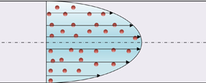
  $\boldsymbol{{\rm H}} = ({H_0},0,0)$ is applied perpendicular to the flow, as shown in figure 1. The components of the linear velocity, microrotation and vorticity are given as $\boldsymbol{U} = (0,0,\bar{\upsilon }(\bar{x}))$, $\boldsymbol{W} = (0,\; \bar{\varOmega }(\bar{x}),0)$ and $\boldsymbol{w} = (0,\bar{\omega }(\bar{x}),0)$, respectively.

Figure 1. Schematic representation of the Poiseuille micropolar flow.
As mentioned above, the MHD micropolar fluid theory of Shizawa & Tanahashi (Reference Shizawa and Tanahashi1986) is used for the study of the present flow. In this model, the constitutive equations of the stress tensor and the couple stress tensor are determined using two thermodynamical conditions, i.e. the second law of thermodynamics is satisfied, while the dissipation function is always positive. Moreover, a constitutive equation for the magnetization is derived with the use of the dissipation function (Aslani et al. Reference Aslani, Benos, Tzirtzilakis and Sarris2020). Then, the governing equations for the present MHD micropolar Poiseuille flow are (Shizawa & Tanahashi Reference Shizawa and Tanahashi1986):
 \begin{gather}\boldsymbol{\nabla }\boldsymbol{\cdot }\boldsymbol{U} = 0,\end{gather}
 \begin{gather}\boldsymbol{\nabla }\boldsymbol{\cdot }\boldsymbol{W} = 0,\end{gather}
 \begin{gather}\boldsymbol{\nabla }\boldsymbol{\cdot }\boldsymbol{B} = 0,\end{gather}
 \begin{gather}\rho \frac{{\textrm{d}\boldsymbol{U}}}{{\textrm{d}\bar{t}}} ={-} \boldsymbol{\nabla }\bar{p} + \eta {\boldsymbol{\nabla }^2}\boldsymbol{U} + 2{\eta _1}\boldsymbol{\nabla } \times (\boldsymbol{W} - \boldsymbol{w}) + \boldsymbol{j} \times \boldsymbol{B} + (\boldsymbol{M}\boldsymbol{\cdot }\boldsymbol{\nabla })\boldsymbol{H} + \boldsymbol{M} \times (\boldsymbol{\nabla } \times \boldsymbol{H}),\end{gather}
 \begin{gather}l\frac{{\textrm{d}\boldsymbol{W}}}{{\textrm{d}\bar{t}}} = \gamma {\nabla ^2}\boldsymbol{W} + 4{\eta _1}(\boldsymbol{w} - \boldsymbol{W}) + \boldsymbol{M} \times \boldsymbol{H},\end{gather}
 \begin{gather}\boldsymbol{w} = \boldsymbol{\nabla } \times \frac{\boldsymbol{U}}{2},\end{gather}
 \begin{gather}\boldsymbol{\nabla } \times \boldsymbol{H} = \boldsymbol{j},\end{gather}
 \begin{gather}\boldsymbol{j} = \sigma (\boldsymbol{E} + \boldsymbol{\upsilon } \times \boldsymbol{B}),\end{gather}
 \begin{gather}\boldsymbol{B} = {\mu _0}\boldsymbol{{\rm H}} + \boldsymbol{{\rm M}},\end{gather}
 \begin{gather}\boldsymbol{M} = \frac{{{M_0}(\boldsymbol{I} - \tau \boldsymbol{W}\boldsymbol{\cdot }\boldsymbol{\varepsilon })\boldsymbol{\cdot }\boldsymbol{H}}}{{\bar{H}}},\end{gather}
where B is the magnetic induction vector,  $\rho $ is the density of the fluid, $\bar{t}$ is the time, $\bar{p}$ is the pressure, $\eta $ is the shear viscosity coefficient, ${\eta _1}$ is the vortex viscosity coefficient, $\boldsymbol{j}$ is the current density, $\boldsymbol{M}$ is the magnetization vector, l is the moment of inertia, $\gamma $ is the angular viscosity coefficient, $\sigma $ is the electrical conductivity, ${\mu _0}$ is the magnetic permeability, ${M_0}$ is the magnetization strength, $\boldsymbol{I}$ is the identical tensor, $\boldsymbol{\varepsilon }$ is the Levi–Civita symbol, $\tau $ is the relaxation time of magnetization and $\bar{H}$ is the magnitude of the magnetic field vector.
The first three equations represent the mass conservation laws and the Gauss law for magnetism. Equations (2.4) and (2.5) are the conservation laws of linear and angular momentum, respectively. Equation (2.6) defines the vorticity. Ampere's and Ohm's laws are depicted in (2.7) and (2.8), respectively. Equations (2.9) and (2.10) represent the constitutive equations for magnetization. The term  $\boldsymbol{M} \times \boldsymbol{H}$ in (2.5) is the MMR term, which is responsible for any magnetization effect on the microrotation.
In the MHD micropolar fluid theory of Shizawa & Tanahashi (Reference Shizawa and Tanahashi1986), the shear viscosity coefficient  $\eta $, the vortex viscosity coefficient ${\eta _1}$, the angular viscosity coefficient $\gamma $, the moment of inertia l and the relaxation time of magnetization $\tau $ are correlated as follows (Shizawa & Tanahashi Reference Shizawa and Tanahashi1986):
 \begin{gather}\gamma = {\iota ^2}\eta ,\end{gather}
 \begin{gather}{\eta _1} = \frac{l}{{4{\tau _s}}},\end{gather}
 \begin{gather}\tau = {\tau _s}(1 + \varepsilon ),\end{gather}
where  ${\iota ^2} = l/\rho $ is the microinertia, ${\tau _s}$ is the relaxation time of microrotation owing to the fluid frictional drag and $\varepsilon $ is the micropolar effect parameter, which is defined as $\varepsilon = {\eta _1}/\eta $ (see (2.38a–e)).
By assuming that no electric field  $\boldsymbol{E}$ is applied on the flow, (2.7) and (2.8) are equalized as follows:
 \begin{equation}\boldsymbol{\nabla } \times \boldsymbol{H} = \sigma (\boldsymbol{\upsilon } \times \boldsymbol{B}).\end{equation}
2.1. Steady-state flow
In the case of the steady-state flow, by analysing the vorticity and the conservation laws of linear and angular momentum (2.4–2.6) in the three directions, we obtain:
 \begin{gather}\bar{\omega } ={-} \frac{1}{2}\frac{{\textrm{d}\bar{\upsilon }}}{{\textrm{d}\bar{x}}},\end{gather}
 \begin{gather}\frac{{\partial \bar{p}}}{{\partial \bar{x}}} = {\bar{j}_y}{\bar{B}_z} + {\bar{M}_z}\frac{{\textrm{d}{{\bar{{\rm H}}}_z}}}{{\textrm{d}\bar{x}}},\end{gather}
 \begin{gather}2(\eta + {\eta _1})\frac{{\textrm{d}\bar{\omega }}}{{\textrm{d}\bar{x}}} - 2{\eta _1}\frac{{\textrm{d}\bar{\varOmega }}}{{\textrm{d}\bar{x}}} + {\bar{j}_y}{\bar{B}_x} ={-} \frac{{\partial \bar{p}}}{{\partial \bar{z}}},\end{gather}
 \begin{gather}\gamma \frac{{{\textrm{d}^2}\bar{\varOmega }}}{{\textrm{d}{{\bar{x}}^2}}} - 4{\eta _1}(\bar{\varOmega } - \bar{\omega }) + {\bar{M}_z}{\bar{{\rm H}}_x} - {\bar{M}_x}{\bar{{\rm H}}_z} = 0.\end{gather}
In this context, the analysis of (2.14) in the  $\bar{x},\bar{y},$ and $\bar{z}$ directions leads to:
 \begin{gather}{\bar{j}_x} = 0,\end{gather}
 \begin{gather}{\bar{j}_y} ={-} \frac{{\textrm{d}{{\bar{{\rm H}}}_z}}}{{\textrm{d}\bar{x}}} = \sigma \bar{\upsilon }{\bar{B}_x},\end{gather}
 \begin{gather}{\bar{j}_z} = 0.\end{gather}
It should be noted that  ${\bar{{\rm H}}_z}$ represents the induced magnetic field, hence, the magnetic field vector is given as $\boldsymbol{H} = ({\bar{{\rm H}}_x},0,{\bar{{\rm H}}_z})$. In this study, the induced magnetic field is assumed to be sufficiently smaller than the applied magnetic field, i.e. ${\bar{H}_z}/{\bar{H}_x} \ll 1$. This is a popular approach, namely the low-magnetic-Reynolds-number approximation $(R{e_m} \ll 1)$, and it has been applied in several investigations (Shizawa et al. Reference Shizawa, Ido and Tanahashi1987a,Reference Shizawa, Ido and Tanahashib; Takashima Reference Takashima1996; Aslani et al. Reference Aslani, Benos, Tzirtzilakis and Sarris2020). This approximation ignores the solution of the magnetic induction equation, which leads to a reduction of the equations to be solved. Thus, the magnetic field vector becomes $\boldsymbol{H} \cong {\bar{{\rm H}}_x}$, which also implies that $\bar{H} \cong {\bar{{\rm H}}_x}$.
With the use of the low- $R{e_m}$ approximation, the magnetization vector $\boldsymbol{M}$ (2.10) is analysed as follows:
 \begin{gather}{\bar{M}_x} = \frac{{{M_0}({{\bar{{\rm H}}}_x} + \tau {{\bar{{\rm H}}}_z}\bar{\varOmega })}}{{{{\bar{{\rm H}}}_x}}} \approx {M_0},\end{gather}
 \begin{gather}{\bar{M}_y} = 0,\end{gather}
 \begin{gather}{\bar{M}_z} = \frac{{{M_0}({{\bar{{\rm H}}}_z} - \tau {{\bar{{\rm H}}}_x}\bar{\varOmega })}}{{{{\bar{{\rm H}}}_x}}} \approx{-} \tau {M_0}\bar{\varOmega }.\end{gather}
Moreover, the magnetic induction vector  $\boldsymbol{B}$ can be analysed as follows:
 \begin{gather}{\bar{B}_x} = {\mu _0}{\bar{{\rm H}}_x} + {\bar{M}_x} \approx {\mu _0}\bar{H} + {M_0},\end{gather}
 \begin{gather}{\bar{B}_y} = 0,\end{gather}
 \begin{gather}{\bar{B}_z} = {\mu _0}{\bar{{\rm H}}_z} + {\bar{M}_z} \approx{-} \tau {M_0}\bar{\varOmega }.\end{gather}
As can be seen from (2.22), the micropolar fluid is permanently magnetized in the  $\bar{x}$ direction with magnetization ${M_0}$. Thus, the continuity of $\boldsymbol{B}$ across the plates requires that ${\bar{B}_x} = {B_0} = {\mu _0}{H_0}$. This leads to the derivation:
 \begin{equation}{\mu _0}{H_0} = {\mu _0}\bar{H} + {M_0},\end{equation}
or,
 \begin{equation}\bar{H} = {H_0} - \frac{{{M_0}}}{{{\mu _0}}}.\end{equation}
Equation (2.29) represents the reduction of the total magnetic field inside the magnetized micropolar fluid (Rosensweig Reference Rosensweig2013).
Subsequently, using all the above-mentioned assumptions, the governing equations can be recast as
 \begin{gather}\bar{\omega } ={-} \frac{1}{2}\frac{{\textrm{d}\bar{\upsilon }}}{{\textrm{d}\bar{x}}},\end{gather}
 \begin{gather}2(\eta + {\eta _1})\frac{{\textrm{d}\bar{\omega }}}{{\textrm{d}\bar{x}}} - 2{\eta _1}\frac{{\textrm{d}\bar{\varOmega }}}{{\textrm{d}\bar{x}}} + {\bar{j}_y}{M_0} + {\mu _0}{\bar{j}_y}\bar{H} = G,\end{gather}
 \begin{gather}\gamma \frac{{{\textrm{d}^2}\bar{\varOmega }}}{{\textrm{d}{{\bar{x}}^2}}} - 4{\eta _1}(\bar{\varOmega } - \bar{\omega }) - \tau {M_0}\bar{\varOmega }\bar{H} = 0.\end{gather}
It should be noted that  $\bar{H}$ is represented by (2.29), while (2.16) is no longer used, as $\partial \bar{p}/\partial \bar{x}$ is associated with the induced magnetic field ${\bar{{\rm H}}_z}$ which is ignored. No-slip boundary conditions are imposed for the linear velocity, while Condiff–Dahler conditions are used for the angular velocity:
 \begin{equation}\bar{\upsilon }( - L) = 0,\quad \bar{\upsilon }(L) = 0,\quad \bar{\varOmega }( - L) = \delta \bar{\omega }( - L),\quad \bar{\varOmega }(L) = \delta \bar{\omega }(L).\end{equation}
The term  $\delta $ is called the wall coefficient. Here, it is assumed that $\delta = 0$, which implies that the microelements adjacent to the channel walls are not able to rotate (Kuemmerer Reference Kuemmerer1978; Borrelli et al. Reference Borrelli, Giantesio and Patria2015; Aslani et al. Reference Aslani, Benos, Tzirtzilakis and Sarris2020).
Equations (2.30)–(2.32) take a non-dimensional form with the use of the following dimensionless terms:
 \begin{equation}\left. {\begin{array}{*{20}{l}} {x = \dfrac{{\bar{x}}}{L},}&{z = \dfrac{{\bar{z}}}{L},}&{\upsilon = \dfrac{{\bar{\upsilon }}}{{{\upsilon_0}}},}&{\varOmega = \dfrac{{\bar{\varOmega }}}{{{\Omega_0}}},}\\ {\omega = \dfrac{{\bar{\omega }}}{{{\omega_0}}},}&{{\rm H} = \dfrac{{\bar{H}}}{{{H_0}}},}&{{\rm M} = \dfrac{{\bar{{\rm M}}}}{{{{\rm M}_0}}},}&{j = \dfrac{{\bar{j}}}{{{j_0}}},} \end{array}} \right\}\end{equation}
where  ${\upsilon _0} = 2G{L^2}/\eta $, ${\varOmega _0} = GL/(2\eta )$, ${\omega _0} = GL/(2\eta )$, ${j_0} = \sigma {\mu _0}{H_0}(2G{L^2}/\eta )$. Hence, the dimensionless governing equations become:
 \begin{gather}\omega ={-} 2\frac{{\textrm{d}\upsilon }}{{\textrm{d}x}},\end{gather}
 \begin{gather}\frac{{\textrm{d}\omega }}{{\textrm{d}x}} - \frac{\varepsilon }{{1 + \varepsilon }}\frac{{\textrm{d}\varOmega }}{{\textrm{d}x}} + \frac{{2H{a^2}}}{{1 + \varepsilon }}\upsilon = \frac{1}{{1 + \varepsilon }},\end{gather}
 \begin{gather}\frac{{{\textrm{d}^2}\varOmega }}{{\textrm{d}{x^2}}} - 4\varepsilon {\lambda ^2}(1 + \zeta (1 - h))\varOmega + 4\varepsilon {\lambda ^2}\omega = 0.\end{gather}
The dimensionless parameters which are introduced in (2.35)–(2.37) are:
 \begin{equation}\varepsilon = \frac{{{\eta _1}}}{\eta },\quad \lambda = \frac{L}{\iota },\quad Ha = {\mu _0}{H_0}L\sqrt {\frac{\sigma }{\eta }} ,\quad \zeta = \frac{{\tau {\tau _s}{H_0}{M_0}}}{l},\quad h = \frac{{{M_0}}}{{{\mu _0}{H_0}}}.\end{equation}
Here,  $\varepsilon $ corresponds to the micropolar effect parameter, $\lambda $ is the size effect parameter and $Ha$ is the Hartmann number. The two new parameters $\zeta $and h are associated with the impact of the magnetization on the micropolar flow. The quantity $\zeta (1 - h)$ in (2.28) is called the magnetization effect parameter $({\sigma _m} = \zeta (1 - h))$ and it is the dimensionless parameter used for the study of the MMR effect. The boundary conditions are written in dimensionless form as follows:
 \begin{equation}\upsilon ( - 1) = 0,\quad \upsilon (1) = 0,\quad \varOmega ( - 1) = 0,\quad \varOmega (1) = 0.\end{equation}
By differentiating (2.36) and using (2.35) and (2.37), a one-way coupled differential equation system is derived as:
 \begin{gather}\frac{{{\textrm{d}^4}\upsilon }}{{\textrm{d}{x^4}}} - {\xi _1}\frac{{{\textrm{d}^2}\upsilon }}{{\textrm{d}{x^2}}} + {\xi _2}\upsilon - {\xi _3} = 0,\end{gather}
 \begin{gather}\varOmega = K\frac{{\textrm{d}\upsilon }}{{\textrm{d}x}} - \varLambda \frac{{{\textrm{d}^3}\upsilon }}{{\textrm{d}{x^3}}}.\end{gather}
The constants  ${\xi _1}$, ${\xi _2}$, ${\xi _3}$, K and $\varLambda $ can be found in Appendix A. The final solutions of the dimensionless velocity and microrotation are:
 \begin{gather}\upsilon = {C_4}{\textrm{e}^{ - Ax}} + {C_3}{\textrm{e}^{Ax}} + {C_2}{\textrm{e}^{ - Bx}} + {C_1}{\textrm{e}^{Bx}} + \frac{{{\xi _3}}}{{{\xi _2}}},\end{gather}
 \begin{gather}\begin{array}{ccccc} \varOmega & ={\textrm{e}^{ - (A + B)x}}( - B{\textrm{e}^{Ax}}({C_2} - {C_1}{\textrm{e}^{2Bx}}){\rm K} + {B^3}{\textrm{e}^{Ax}}({C_2} - {C_1}{\textrm{e}^{2Bx}})\varLambda \\ & + \; A{\textrm{e}^{Bx}}({C_4} - {C_3}{\textrm{e}^{2Ax}})( - {\rm K} + {A^2}\varLambda )). \end{array}\end{gather}
All variables appearing in (2.42) and (2.43) are included in Appendix A.
The skin friction coefficient of the flow can be generally defined as (Kim & Kim Reference Kim and Kim2004)
 \begin{equation}{C_f} = \frac{{2{{\bar{\tau }}_w}}}{{\rho {\upsilon _0}^2}},\end{equation}
where  ${\bar{\tau }_w}$ is the shear stress, which, according to Shizawa & Tanahashi (Reference Shizawa and Tanahashi1986) and Shizawa et al. (Reference Shizawa, Ido and Tanahashi1987a), can be interpreted as
 \begin{equation}{\bar{\tau }_w} = (\eta + {\eta _1})\frac{{\textrm{d}\bar{\upsilon }}}{{\textrm{d}\bar{x}}} + 2{\eta _1}\bar{\varOmega }.\end{equation}
Τhe shear stress can be non-dimensionalized by introducing the associated dimensionless shear stress variable as  ${\bar{\tau }_w} = {\tau _w}/{\tau _0}$, where ${\tau _0} = \eta {\upsilon _0}/2L$. Considering the latter and the dimensionless variables defined in (2.34) and (2.38a–e), the shear stress can be written as
 \begin{equation}{\tau _w} = 2(1 + \varepsilon )\frac{{\textrm{d}\upsilon }}{{\textrm{d}x}} + \varepsilon \varOmega .\end{equation}
In this case, the skin friction coefficient for the lower plate takes the form:
 \begin{equation}{C_f} = R{e^{ - 1}}\left( {2(1 + \varepsilon ){{\left. {\frac{{\textrm{d}\upsilon }}{{\textrm{d}x}}} \right|}_{x ={-} 1}} + \varepsilon {{ \varOmega |}_{x ={-} 1}}} \right),\end{equation}
where  $Re = \rho {\upsilon _0}L/\eta $ is the Reynolds number.
2.2. Stability analysis
In this study, the linear stability of the MHD micropolar Poiseuille flow is performed by assuming an infinitesimal disturbance on the initial state of the flow, as follows:
 \begin{equation}\left. {\begin{array}{*{20}{c@{}}} {{{\bar{u}}_x} = \bar{u} + {{\bar{u}}_{xf}},\quad {{\bar{u}}_z} = \bar{\upsilon } + {{\bar{u}}_{zf}},\quad \bar{W} = \bar{\varOmega } + {{\bar{\varOmega }}_f},\quad \bar{P} = \bar{p} + {{\bar{p}}_f},}\\ {\bar{j} = {{\bar{j}}_y} + {{\bar{j}}_{yf}},\quad {{\bar{b}}_x} = {{\bar{B}}_x} + {{\bar{B}}_{xf}},\quad {{\bar{b}}_z} = {{\bar{B}}_z} + {{\bar{B}}_{zf}},\quad {{\bar{h}}_x} = {{\bar{H}}_x} + {{\bar{H}}_{xf}},}\\ {{{\bar{h}}_z} = {{\bar{H}}_z} + {{\bar{H}}_{zf}},\quad {{\bar{m}}_x} = {{\bar{M}}_x} + {{\bar{M}}_{xf}},\quad {{\bar{m}}_z} = {{\bar{M}}_z} + {{\bar{M}}_{zf}}.} \end{array}} \right\}\end{equation}
Here,  ${\bar{u}_x}$ and ${\bar{u}_z}$ are the dimensional perturbed velocities in the $\bar{x}$ and $\bar{z}$ directions, respectively, ${\bar{b}_x}$ and ${\bar{b}_z}$ are the dimensional perturbed magnetic flux density components in the $\bar{x}$ and $\bar{z}$ directions, respectively, ${\bar{h}_x}$ and ${\bar{h}_z}$ are the dimensional perturbed magnetic field components in the $\bar{x}$ and $\bar{z}$ directions, respectively, ${\bar{m}_x}$ and ${\bar{m}_z}$ are the dimensional perturbed magnetization components in the $\bar{x}$ and $\bar{z}$ directions, respectively, and $\bar{W}$, $\bar{P}$ and $\bar{j}$ are the dimensional perturbed microrotation, pressure and current density, respectively. Additionally, $\bar{u} = 0$, while $\bar{\upsilon }$ and $\bar{\varOmega }$ are the base velocity and microrotation states, as they were derived in (2.42) and (2.43). Squire's theorem (Drazin & Reid Reference Drazin and Reid2004) is valid and only 2-D disturbances in the $\bar{z} - \bar{x}$ plane are considered, i.e. ${\bar{u}_{xf}}(\bar{x},\bar{z},\bar{t})$, ${\bar{u}_{zf}}(\bar{x},\bar{z},\bar{t})$ and ${\bar{\varOmega }_f}(\bar{x},\bar{z},\bar{t})$. Then, the dimensional perturbed governing equations are:
 \begin{gather}{\bar{j}_{yf}} = \sigma ({\bar{u}_{zf}}{\bar{B}_x} + \bar{\upsilon }{\bar{B}_{xf}} - {\bar{u}_{xf}}{\bar{B}_z}),\end{gather}
 \begin{gather}{\bar{M}_{xf}} = 0,\end{gather}
 \begin{gather}{\bar{M}_{zf}} ={-} \tau {M_0}{\bar{\varOmega }_f},\end{gather}
 \begin{gather}
\rho \left( {\dfrac{{\partial {{\bar{u}}_{xf}}}}{{\partial
\bar{t}}} + \bar{\upsilon }\dfrac{{\partial
{{\bar{u}}_{xf}}}}{{\partial \bar{z}}}} \right) =-
\dfrac{{\partial {{\bar{p}}_f}}}{{\partial \bar{x}}} + \eta
\left( {\dfrac{{{\partial^2}{{\bar{u}}_{xf}}}}{{\partial
{{\bar{x}}^2}}} +
\dfrac{{{\partial^2}{{\bar{u}}_{xf}}}}{{\partial
{{\bar{z}}^2}}}} \right) + {\eta _1}\left(
{\dfrac{{{\partial^2}{{\bar{u}}_{xf}}}}{{\partial
{{\bar{z}}^2}}} -
\dfrac{{{\partial^2}{{\bar{u}}_{zf}}}}{{\partial
\bar{z}\partial \bar{x}}}} \right)\notag\\ - \; 2{\eta
_1}\dfrac{{\partial {{\bar{\varOmega }}_f}}}{{\partial
\bar{z}}} + {\mu _0}({{\bar{j}}_y}{{\bar{H}}_{zf}} +
{{\bar{j}}_{yf}}{{\bar{H}}_z}) +
{{\bar{M}}_x}\dfrac{{\partial {{\bar{H}}_{xf}}}}{{\partial
\bar{x}}} + {{\bar{M}}_z}\dfrac{{\partial
{{\bar{H}}_{xf}}}}{{\partial \bar{z}}},
\end{gather}
\begin{gather}
\rho \left( {\dfrac{{\partial {{\bar{u}}_{xf}}}}{{\partial
\bar{t}}} + \bar{\upsilon }\dfrac{{\partial
{{\bar{u}}_{xf}}}}{{\partial \bar{z}}}} \right) =-
\dfrac{{\partial {{\bar{p}}_f}}}{{\partial \bar{x}}} + \eta
\left( {\dfrac{{{\partial^2}{{\bar{u}}_{xf}}}}{{\partial
{{\bar{x}}^2}}} +
\dfrac{{{\partial^2}{{\bar{u}}_{xf}}}}{{\partial
{{\bar{z}}^2}}}} \right) + {\eta _1}\left(
{\dfrac{{{\partial^2}{{\bar{u}}_{xf}}}}{{\partial
{{\bar{z}}^2}}} -
\dfrac{{{\partial^2}{{\bar{u}}_{zf}}}}{{\partial
\bar{z}\partial \bar{x}}}} \right)\notag\\ - \; 2{\eta
_1}\dfrac{{\partial {{\bar{\varOmega }}_f}}}{{\partial
\bar{z}}} + {\mu _0}({{\bar{j}}_y}{{\bar{H}}_{zf}} +
{{\bar{j}}_{yf}}{{\bar{H}}_z}) +
{{\bar{M}}_x}\dfrac{{\partial {{\bar{H}}_{xf}}}}{{\partial
\bar{x}}} + {{\bar{M}}_z}\dfrac{{\partial
{{\bar{H}}_{xf}}}}{{\partial \bar{z}}},
\end{gather} \begin{gather} \rho
\left( {\dfrac{{\partial {{\bar{u}}_{zf}}}}{{\partial
\bar{t}}} + {{\bar{u}}_{xf}}\dfrac{{\partial \bar{\upsilon
}}}{{\partial \bar{x}}} + \bar{\upsilon }\dfrac{{\partial
{{\bar{u}}_{zf}}}}{{\partial \bar{z}}}} \right) =-
\dfrac{{\partial {{\bar{p}}_f}}}{{\partial \bar{z}}} + \eta
\left( {\dfrac{{{\partial^2}{{\bar{u}}_{zf}}}}{{\partial
{{\bar{x}}^2}}} +
\dfrac{{{\partial^2}{{\bar{u}}_{zf}}}}{{\partial
{{\bar{z}}^2}}}} \right) + 2{\eta _1}\dfrac{{\partial
{{\bar{\varOmega }}_f}}}{{\partial \bar{x}}}\notag\\ + \; {\eta
_1}\left( {\dfrac{{{\partial^2}{{\bar{u}}_{zf}}}}{{\partial
{{\bar{x}}^2}}} -
\dfrac{{{\partial^2}{{\bar{u}}_{xf}}}}{{\partial
\bar{x}\partial \bar{z}}}} \right) - {\mu
_0}({{\bar{j}}_y}{{\bar{H}}_{xf}} +
{{\bar{j}}_{yf}}{{\bar{H}}_x})\notag\\ +
{{\bar{M}}_z}\dfrac{{\partial {{\bar{H}}_{zf}}}}{{\partial
\bar{z}}} + {{\bar{M}}_x}\dfrac{{\partial
{{\bar{H}}_{zf}}}}{{\partial \bar{x}}} +
{{\bar{M}}_{xf}}\dfrac{{\partial {{\bar{H}}_z}}}{{\partial
\bar{x}}},
\end{gather}
\begin{gather} \rho
\left( {\dfrac{{\partial {{\bar{u}}_{zf}}}}{{\partial
\bar{t}}} + {{\bar{u}}_{xf}}\dfrac{{\partial \bar{\upsilon
}}}{{\partial \bar{x}}} + \bar{\upsilon }\dfrac{{\partial
{{\bar{u}}_{zf}}}}{{\partial \bar{z}}}} \right) =-
\dfrac{{\partial {{\bar{p}}_f}}}{{\partial \bar{z}}} + \eta
\left( {\dfrac{{{\partial^2}{{\bar{u}}_{zf}}}}{{\partial
{{\bar{x}}^2}}} +
\dfrac{{{\partial^2}{{\bar{u}}_{zf}}}}{{\partial
{{\bar{z}}^2}}}} \right) + 2{\eta _1}\dfrac{{\partial
{{\bar{\varOmega }}_f}}}{{\partial \bar{x}}}\notag\\ + \; {\eta
_1}\left( {\dfrac{{{\partial^2}{{\bar{u}}_{zf}}}}{{\partial
{{\bar{x}}^2}}} -
\dfrac{{{\partial^2}{{\bar{u}}_{xf}}}}{{\partial
\bar{x}\partial \bar{z}}}} \right) - {\mu
_0}({{\bar{j}}_y}{{\bar{H}}_{xf}} +
{{\bar{j}}_{yf}}{{\bar{H}}_x})\notag\\ +
{{\bar{M}}_z}\dfrac{{\partial {{\bar{H}}_{zf}}}}{{\partial
\bar{z}}} + {{\bar{M}}_x}\dfrac{{\partial
{{\bar{H}}_{zf}}}}{{\partial \bar{x}}} +
{{\bar{M}}_{xf}}\dfrac{{\partial {{\bar{H}}_z}}}{{\partial
\bar{x}}},
\end{gather} \begin{gather}
l\left( {\dfrac{{\partial {{\bar{\varOmega
}}_f}}}{{\partial \bar{t}}} +
{{\bar{u}}_{xf}}\dfrac{{\partial \bar{\varOmega
}}}{{\partial \bar{x}}} + \bar{\upsilon }\dfrac{{\partial
{{\bar{\varOmega }}_f}}}{{\partial \bar{z}}}} \right)
=\gamma \left( {\dfrac{{{\partial^2}{{\bar{\varOmega
}}_f}}}{{\partial {{\bar{x}}^2}}} +
\dfrac{{{\partial^2}{{\bar{\varOmega }}_f}}}{{\partial
{{\bar{z}}^2}}}} \right) + 2{\eta _1}\left(
{\dfrac{{\partial {{\bar{u}}_{xf}}}}{{\partial \bar{z}}} -
\dfrac{{\partial {{\bar{u}}_{zf}}}}{{\partial \bar{x}}} -
2{{\bar{\varOmega }}_f}} \right)\notag\\ + \;
{{\bar{M}}_z}{{\bar{H}}_{xf}} +
{{\bar{M}}_{zf}}{{\bar{H}}_x} -
({{\bar{M}}_x}{{\bar{H}}_{zf}} +
{{\bar{M}}_{xf}}{{\bar{H}}_z}).
\end{gather}
\begin{gather}
l\left( {\dfrac{{\partial {{\bar{\varOmega
}}_f}}}{{\partial \bar{t}}} +
{{\bar{u}}_{xf}}\dfrac{{\partial \bar{\varOmega
}}}{{\partial \bar{x}}} + \bar{\upsilon }\dfrac{{\partial
{{\bar{\varOmega }}_f}}}{{\partial \bar{z}}}} \right)
=\gamma \left( {\dfrac{{{\partial^2}{{\bar{\varOmega
}}_f}}}{{\partial {{\bar{x}}^2}}} +
\dfrac{{{\partial^2}{{\bar{\varOmega }}_f}}}{{\partial
{{\bar{z}}^2}}}} \right) + 2{\eta _1}\left(
{\dfrac{{\partial {{\bar{u}}_{xf}}}}{{\partial \bar{z}}} -
\dfrac{{\partial {{\bar{u}}_{zf}}}}{{\partial \bar{x}}} -
2{{\bar{\varOmega }}_f}} \right)\notag\\ + \;
{{\bar{M}}_z}{{\bar{H}}_{xf}} +
{{\bar{M}}_{zf}}{{\bar{H}}_x} -
({{\bar{M}}_x}{{\bar{H}}_{zf}} +
{{\bar{M}}_{xf}}{{\bar{H}}_z}).
\end{gather}
It should be noted that the vorticity  $\boldsymbol{w}$ in the perturbed governing equations (2.49)–(2.54) has been replaced by (2.6). Considering that the magnetic Reynolds number is very small, and following the steps of Takashima (Reference Takashima1996), the magnetic Prandtl number ${P_m} = R{e_m}/Re$ is also very small and, thus, the terms involving ${\bar{H}_z}$ can be ignored, while $\bar{H} \cong {\bar{{\rm H}}_x}$. Moreover, the total magnetic field $\bar{H}$ inside the magnetized micropolar fluid is given in (2.29).
A disturbance streamfunction with wavenumber  $\bar{\alpha }$ and frequency $\bar{c}$ is introduced as follows:
 \begin{equation}\bar{\psi }(\bar{x},\bar{z},\bar{t}) = \bar{\varphi }(\bar{x})\,{\textrm{e}^{\textrm{i}\bar{\alpha }(\bar{z} - \bar{c}\bar{t})}},\end{equation}
where  ${\bar{u}_{xf}} ={-} (\partial \bar{\psi }/\partial \bar{z})$, ${\bar{u}_{zf}} = \partial \bar{\psi }/\partial \bar{x}$, and $\textrm{i}$ is the imaginary unit.
The corresponding microrotation disturbance is
 \begin{equation}{\bar{\varOmega }_f}(\bar{x},\bar{z},\bar{t}) = \bar{w}(\bar{x})\,{\textrm{e}^{\textrm{i}\bar{\alpha }(\bar{z} - \bar{c}\bar{t})}}.\end{equation}
The wavenumber  $\bar{\alpha }$ and the frequency $\bar{c}$ are assumed to be periodic in space, where $\bar{\alpha }$ is real and is able to decay or grow with time, while $\bar{c} = {\bar{c}_r} + \textrm{i}{\bar{c}_i}$ is complex. The parameter ${\bar{c}_r}$ represents the disturbance wave propagation speed and ${\bar{c}_i}$ is the temporal amplification coefficient. When ${\bar{c}_i} < 0$, the disturbance decays and the flow is stable, while for ${\bar{c}_i} > 0$, the disturbance grows and the flow becomes unstable. The objective here is to derive ${\bar{c}_i}$ as a function of $\bar{\alpha }$ for various values of the dimensionless parameters associated with the flow (see (2.38a–e)). In this manner, the boundary conditions for the perturbed flow are
 \begin{equation}\bar{\varphi }({\pm} L) = 0,\quad \frac{{\partial \bar{\varphi }}}{{\partial \bar{x}}}({\pm} L) = 0,\quad \bar{w}({\pm} L) = 0.\end{equation}
The perturbed governing equations can be non-dimensionalized using the dimensionless variables from (2.34) and (2.38a–e) and introducing new ones, as follows:
 \begin{equation}\alpha = \bar{\alpha }L,\quad c = \frac{{\bar{c}}}{{{\upsilon _0}}},\quad \varphi = \frac{{\bar{\varphi }}}{{{\upsilon _0}L}},\quad w = \bar{w}\frac{{4L}}{{{\upsilon _0}}}.\end{equation}
where  ${\upsilon _0} = 2G{L^2}/\eta .$ Then, the resulting dimensionless perturbed equation system is
 \begin{gather}\begin{array}{ccccc} & \dfrac{1}{{\textrm{i}\alpha Re}}\left[ {(1 + \varepsilon )\left( {\dfrac{{{\partial^4}\varphi }}{{\partial {x^4}}} - 2{\alpha^2}\dfrac{{{\partial^2}\varphi }}{{\partial {x^2}}} + {\alpha^4}\varphi } \right) + \dfrac{\varepsilon }{2}\left( {\dfrac{{{\partial^2}w}}{{\partial {x^2}}} - {\alpha^2}w} \right) - H{a^2}(1 - h)\dfrac{{{\partial^2}\varphi }}{{\partial {x^2}}}} \right]\\ & \quad = (\upsilon - c)\left( {\dfrac{{{\partial^2}\varphi }}{{\partial {x^2}}} - {\alpha^2}\varphi } \right) - \dfrac{{{\partial ^2}\upsilon }}{{\partial {x^2}}}\varphi , \end{array}\end{gather}
 \begin{gather}\begin{array}{ccccc} & \dfrac{1}{{\textrm{i}\alpha Re}}\left[ {\left( {\dfrac{{{\partial^2}w}}{{\partial {x^2}}} - {\alpha^2}w} \right) - 8\varepsilon {\lambda^2}\left( {\dfrac{1}{2}w + \dfrac{{{\partial^2}\varphi }}{{\partial {x^2}}} - {\alpha^2}\varphi } \right) - 4\varepsilon {\lambda^2}{\sigma_m}w} \right]\\ & \quad = (\upsilon - c)w - \dfrac{{\partial \Omega }}{{\partial x}}\varphi , \end{array}\end{gather}
with the following dimensionless boundary conditions:
 \begin{equation}\varphi ({\pm} 1) = 0,\quad \frac{{\partial \varphi }}{{\partial x}}({\pm} 1) = 0,\quad w({\pm} 1) = 0.\end{equation}
The system of the sixth-order perturbed equations (2.59–2.60) constitutes a modified version of the Orr–Sommerfeld equation. These equations appear to have the same form as equations (13) and (14) in the micropolar stability study of Kuemmerer (Reference Kuemmerer1978), including two extra terms. The first term is the second derivative of  $\varphi $ multiplied by the Hartmann number $Ha$ and the parameter $h$, as seen in (2.59). This term is associated with the stability effects of the applied magnetic field and the magnetization on the fluid velocity as it appears in (2.44) of the MHD stability study of Takashima (Reference Takashima1996). The second term involves the variable w multiplied by the micropolar effect parameter $\varepsilon $, the size effect parameter $\lambda $ and the magnetization effect parameter ${\sigma _m}$, as seen in (2.60). This term is derived for the first time and involves the stabilizing effect of the MMR on the MHD micropolar Poiseuille flow.
In many stability studies associated with the Orr–Sommerfeld equation or its modified versions, the Chebyshev collocation method is employed for the solution of the perturbed equations (Orszag Reference Orszag1971; Takashima Reference Takashima1993, Reference Takashima1996; Liu et al. Reference Liu, Liu and Zhao2008; Essaghir et al. Reference Essaghir, Haddout, Oubarra and Lahjomri2016; Shankar, Kumar & Shivakumara Reference Shankar, Kumar and Shivakumara2017). The discretization of the stability equations in N collocation points results in a linear algebraic equation system:
 \begin{equation}\boldsymbol{AX} = c\boldsymbol{BX}.\end{equation}
For fixed values of the dimensionless parameters along with the Reynolds number  $Re$ and the wavenumber $\alpha $, the frequency c can be obtained as the eigenvalues of the matrix ${\boldsymbol{B}^{ - 1}}\boldsymbol{A}$. From N eigenvalues $c(1),c(2), \ldots ,c(N)$, the one with the largest imaginary part ( $c(K)$, say) is chosen. To derive the neutral stability curves, the value of the Reynolds number $Re$ for which the imaginary part of $c(K)$ is zero must be selected. When $\boldsymbol{B}$ is singular, the QZ algorithm of Moler & Stewart (Reference Moler and Stewart1973) is used for the solution of the eigenvalue problem.
In the present study, the free open-source numerical software ‘Chebfun’ and ‘Chebop’, initially developed by Z. Battles and L.N. Trefethen of Oxford University, is employed (Battles & Trefethen Reference Battles and Trefethen2004). The fifth version of this software (Chebfun v5), used for the numerical solution of the difficult eigenvalue problem, uses Chebyshev expansion coefficients to sufficiently discretize complicated functions that require even 1 000 000 points. Chebfun implements adaptive procedures to detect the correct number of points automatically. This procedure results in a highly accurate representation of functions, with an accuracy of up to 15 digits (Driscoll, Hale & Trefethen Reference Driscoll, Hale and Trefethen2014). Chebop is a differential or integral operator that acts on Chebfun and it is employed to solve differential equations such as the Orr–Sommerfeld equation (Essaghir et al. Reference Essaghir, Haddout, Oubarra and Lahjomri2016). Once the modified Orr–Sommerfeld equations (2.59)–(2.60) along with the corresponding boundary conditions (2.61a–c) are implemented in Chebop code, the frequency c eigenvalues are obtained with the use of the command ‘eigs’ in MATLAB. This command is built on the QZ algorithm and it is suitable for the solution of singular matrices. Finally, a code based on the bisection method was used for the derivation of the neutral stability curves.
3. Results and discussion
In this study, the problem of the MMR effect on an MHD micropolar Poiseuille flow is examined. As was shown in § 2, two dimensionless parameters,  $\zeta $ and h are associated with the impact of magnetization on the flow. These two parameters are combined in the magnetization effect parameter ${\sigma _m} = \zeta (1 - h)$. When ${\sigma _m} = 0$, i.e. $\zeta = 0$ and/or $h = 1$, the MMR term is negated and the theory of Shizawa & Tanahashi (Reference Shizawa and Tanahashi1986) is reduced to Eringen's MHD micropolar fluid model. To specify the MMR effect on the flow, the velocity and microrotation are presented for various values of the associated dimensionless parameters for ${\sigma _m} = 0$ and 1. In the case of ${\sigma _m} = 1$, it is assumed that $\zeta = 2$ and $h = 0.5$ while for ${\sigma _m} = 0$, $\zeta = 0$ and $h = 0$ are considered. The impact of MMR on the velocity $\upsilon $ and microrotation $\varOmega $ profiles is clearly illustrated by the induced relative errors $\mathrm{\Delta }\upsilon $ and $\mathrm{\Delta }\varOmega $, by switching on and off the magnetization effect parameter ${\sigma _m}$, while keeping the other dimensionless parameters fixed. The relative differences $\mathrm{\Delta }\upsilon $ and $\mathrm{\Delta }\varOmega $ are defined as follows:
 \begin{gather}\mathrm{\Delta }\upsilon (\%) = \frac{{{\upsilon _{{\sigma _m} = 1}} - {\upsilon _{{\sigma _m} = 0}}}}{{{\upsilon _{{\sigma _m} = 0}}}} \times 100,\end{gather}
 \begin{gather}\mathrm{\Delta }\varOmega (\%) = \frac{{{\varOmega _{{\sigma _m} = 1}} - {\varOmega _{{\sigma _m} = 0}}}}{{{\varOmega _{{\sigma _m} = 0}}}} \times 100.\end{gather}
Considering all the above, the effect of the MMR term on the base velocity and microrotation states is discussed below.
3.1. Steady-state flow
3.1.1. Effect of MMR on the flow for various values of micropolar effect parameter  $\varepsilon $

The micropolar effect parameter,  $\varepsilon $, is the ratio of the vortex viscosity coefficient to the Newtonian kinematic viscosity. It varies in the range $0 < \varepsilon < 1$. When $\varepsilon \to 0$, the classical equations for the Newtonian fluid flow are retrieved, while as $\varepsilon $ increases, the fluid internal microstructure becomes denser (Borrelli et al. Reference Borrelli, Giantesio and Patria2015). Thus, $\varepsilon $ represents a measure of the micropolar diffusion over molecular dissipation (Aslani et al. Reference Aslani, Benos, Tzirtzilakis and Sarris2020).
The influence of the MMR term on the dimensionless velocity  $\upsilon $ and microrotation $\varOmega $ distributions is presented in figure 2, when $\varepsilon = 0.2,\;0.5$ and 0.8, for $\lambda = 5$ and $Ha = 1$. It can be seen that as $\varepsilon $ increases, the flow is slightly decelerated, while the microrotation is increased. The consideration of the magnetization parameter, ${\sigma _m}$, differentiates further the velocity and microrotation profiles. A significant observation on the velocity field (figure 2(a–c), left side) is that, for small $\varepsilon $ values, the magnetization does not seem to have a noticeable effect, but as $\varepsilon $ increases, magnetization starts to affect the fluid velocity. This occurs because, when small $\varepsilon $ values are considered, the velocity field is similar to that of a Newtonian fluid. However, when $\varepsilon $ increases, the microrotation is enhanced and the MMR term appears to have a stronger impact on the flow.

Figure 2. Effect of  ${\sigma _m}$ on velocity (left) and microrotation (right) for $\lambda = 5$, $Ha = 1$ and $\varepsilon $ equal to: (a) 0.2 (top), (b) 0.5 (middle), and (c) 0.8 (bottom).
The effect of the magnetization on microrotation is depicted in figure 2(a–c) (right side). It is obvious that when  ${\sigma _m} = 1$, microrotation is reduced as $\varepsilon $ increases, and its maximum value approaches the walls resulting in a narrower boundary layer. In this manner, the MMR term seems to enhance the dissipation in a similar way to that of an increasing magnetic field (Pothérat & Klein Reference Pothérat and Klein2017). It appears that the magnetic energy, which usually has a braking effect on the flow, is transferred directly via the Lorentz force and the micromagnetorotation to the linear and angular momentums, respectively. It should be noted, that when the MMR term is ignored, i.e. ${\sigma _m} = 0$, the magnetic energy has a direct influence only on the velocity via the Lorentz force and on the microrotation indirectly, via the velocity.
The relative differences for the velocity and microrotation fields for  ${\sigma _m} = 0$ and 1, in the cases of $\varepsilon = 0.2,\;0.5$ and 0.8, are demonstrated in figures 3(a) and 3(b), respectively. As already mentioned, the MMR term tends to decelerate the flow. The flow reduction increases as it moves away from the plates and reaches a maximum at the centre of the channel. The relative reductions increase as $\varepsilon $ increases, approaching the value of 16 % for the velocity and 61 % for microrotation when $\varepsilon = 0.8$. It seems that the dual action of the magnetic field via the Lorentz force and the MMR term has a braking impact, which results in an analogous deceleration of the flow.

Figure 3. Relative difference in (a) velocity  $\mathrm{\Delta }\upsilon $, and (b) microrotation $\mathrm{\Delta }\varOmega $ between ${\sigma _m} = 0$ and 1, for $\varepsilon = 0.2$, 0.5 and 0.8, $\lambda = 5$ and $Ha = 1$.
3.1.2. Effect of MMR on the flow for various values of size effect parameter $\lambda $

The size effect parameter,  $\lambda = L/\iota $, is associated with the geometry of the flow, through the channel half-height, L, and the microinertia, $\iota $, which is also related to the angular viscosity coefficient $\gamma $, because $\gamma = {\iota ^2}\eta $. As mentioned by Shizawa et al. (Reference Shizawa, Ido and Tanahashi1987a,Reference Shizawa, Ido and Tanahashib), the size effect parameter is defined in the range $5 \le \lambda < \infty $. Physically, a greater value of $\lambda $ will result in smaller particles in the micropolar fluid. Moreover, as $\lambda \to \infty $ for constant L, the angular viscosity coefficient $\gamma $ decreases, which indicates smaller values of fluid–particle resistance.
In the same manner as in the previous subsection, figure 4 illustrates the velocity and microrotation profiles for  $\lambda = 5,\;9$ and 13, when $\varepsilon = 0.1$ and $Ha = 1$, for the cases of ${\sigma _m} = 0$ and $1$. It is obvious that as $\lambda $ increases, both velocity and microrotation appear to have a small growth, which is more noticeable for the microrotation. The MMR term has a smaller effect on the flow for growing values of $\lambda $, compared with the corresponding effect for increasing values of $\varepsilon $. Again, the magnetization effect on the microrotation is stronger compared with on the velocity. This situation can be explained by the impact of $\lambda $ on the micropolar flow. When $\lambda $ increases, there is smaller resistance between the rigid particles and the fluid, which enhances their independent rotation, i.e. the microrotation field. As a result, the MMR term has a stronger effect on the microrotation with growing $\lambda $, while it affects the velocity indirectly, via the microrotation. When ${\sigma _m} = 1$, both velocity and microrotation are reduced. The braking effect of the flow, owing to the dual energy of the magnetic field, is more intense for the microrotation field because of the MMR effect, when ${\sigma _m} = 1$ is considered.

Figure 4. Effect of  ${\sigma _m}$ on velocity (left) and microrotation (right) for $\varepsilon = 0.1$, $Ha = 1$ and $\lambda $ equal to: (a) 5 (top), (b) 9 (middle), and (c) 13 (bottom).
Figure 5 presents the relative differences for the velocity and microrotation when  $\lambda = 5,\;9$ and 13, for ${\sigma _m} = 0$ and 1. The difference in both profiles for $\lambda $ are similar to the corresponding ones for $\varepsilon $. As $\lambda $ grows, the relative differences are increased. Again, both $\mathrm{\Delta }\upsilon $ and $\mathrm{\Delta }\varOmega $ grow smoothly across the channel, while they have a maximum value at the centre of the channel, i.e. $x = 0$. These values are $- 2.3\,\%$ for $\mathrm{\Delta }\upsilon $ and $- 51\,\%$ for $\mathrm{\Delta }\varOmega $, when $\lambda = 13$. It is obvious that the MMR term is associated with a faster rotation of the suspended bodies in the fluid with increasing $\lambda $, which leads to a faster dissipation of the kinetic energy.

Figure 5. Relative difference in (a) velocity  $\mathrm{\Delta }\upsilon $, and (b) microrotation, $\mathrm{\Delta }\varOmega $, between ${\sigma _m} = 0$ and 1, for $\lambda = 5$, 9 and 13, for $\varepsilon = 0.1$ and $Ha = 1$.
3.1.3. Effect of MMR on the flow for various values of Hartmann number $Ha$

The Hartmann number  $Ha$ is a dimensionless parameter associated with the MHD effect and the strength of the applied magnetic field. It can take any value in the range $0 \le Ha < \infty $. For $Ha = 0$, no magnetic field is applied to the flow, while as $Ha$ increases, the applied magnetic field becomes stronger. In this manner, the effect of the applied magnetic field on the velocity and microrotation is depicted in figure 6, for $Ha = 0.1,1.5,3$ and 20, when $\varepsilon = 0.4$ and $\lambda = 5$, for the cases of ${\sigma _m} = 0$ and 1. Similarly to the classical MHD Poiseuille flow (Takashima Reference Takashima1996), the increase of $Ha$ leads to a significant decrease of the fluid velocity and microrotation. An important result here is that for $Ha$ values greater than 3, both velocity and microrotation decrease rapidly. When $Ha = 20$, the order of magnitude of the velocity and microrotation is ${10^{ - 3}}$, which is practically zero. The decrease in the velocity of the micropolar flow with increasing $Ha$ is greater compared with the corresponding velocity decrease of a Newtonian flow.

Figure 6. Effect of  ${\sigma _m}$ on velocity (left) and microrotation (right) for $\varepsilon = 0.4$, $\lambda = 5$ and $Ha$ equal to: (a) 0.1, (b) 1.5, (c) 3, and (d) 20.
When the MMR effect is considered, both velocity and microrotation are further reduced. This situation confirms that the MMR term acts in a similar way as the Lorentz force by having a braking effect on the flow. The Lorentz force has a direct influence on the fluid velocity, while it affects the microrotation via the velocity. However, the MMR diminishes the microrotation directly, which further reduces the fluid velocity. The phenomenon associated with the ‘freezing’ of an MHD flow is called Hartmann braking and it is observed in various industrial applications that involve magnetic fields, such as the liquid metal blankets of nuclear fusion reactors (Aslani et al. Reference Aslani, Benos, Tzirtzilakis and Sarris2020).
Figure 7 illustrates the relative differences for the velocity and microrotation fields, when  ${\sigma _m} = 0$ and 1, for the cases of $Ha = 0.1,\;1.5,\;3$ and 20. It is obvious that as $Ha$ increases and the velocity decreases, the effect of magnetization on the velocity field is reduced. When $Ha = 0.1$, the velocity relative difference $\mathrm{\Delta }\upsilon $ has a maximum value of $- \; 10\,\%$ at $x = 0$. For the case of $Ha = 20$, $\mathrm{\Delta }\upsilon $ is almost zero across the channel. Similarly, when $Ha$ increases from 0.1 to 3, the MMR effect decreases slightly. For $Ha = 0.1,\;1,\;1.5$ and 3, the microrotation relative difference $\mathrm{\Delta }\varOmega $ has a maximum value of approximately $- 50\,\%$. This situation indicates that the intense velocity decrease has a small impact on $\mathrm{\Delta }\varOmega $. Interestingly, for $Ha = 20$, the microrotation relative difference increases rapidly, reaching the value of $- 89\,\%$ at $x = 0$. In this case, the MMR effect on the microrotation field is so strong that it prevails over the ‘freezing’ of the flow velocity. Thus, the microrotation relative difference is maximized.

Figure 7. Relative difference in (a) velocity  $\mathrm{\Delta }\upsilon $, and (b) microrotation, $\Delta \varOmega$, between ${\sigma _m} = 0$ and 1 for $Ha = 0.1$, 1.5, 3 and 20, for $\varepsilon = 0.4$ and $\lambda = 5$.
3.1.4. Effect of MMR on skin friction coefficient ${C_f}$

In this study, the skin friction coefficient  ${C_f}$ has been calculated at the lower plate of the MHD micropolar Poiseuille flow for various values of the Reynolds number $Re$. Consequently, the derived ${C_f}$ values are compared with the corresponding ones of the classical Newtonian Poiseuille flow, the classical Newtonian MHD Poiseuille flow, the simple micropolar Poiseuille flow and the MHD micropolar Poiseuille flow by ignoring the MMR term, i.e., for ${\sigma _m} = 0$. The ${C_f}$ for the classical Newtonian Poiseuille flow is ${C_{{\,f_{Newt.}}}} = 1/Re$. The steady-state solution for the velocity profile of the Newtonian Poiseuille flow is derived from Drazin & Riley (Reference Drazin and Riley2006). The velocity profile for the Newtonian MHD Poiseuille flow was obtained from Takashima (Reference Takashima1993) and the skin friction coefficient of this case is found to be ${C_{{\,f_{MHD}}}} = R{e^{ - 1}}H{a^{ - 1}}[( - 1 + {\textrm{e}^{2Ha}})/(1 + {\textrm{e}^{2Ha}})]$. It should be noted that the same dimensionless parameters defined in (2.34) are used for the calculation of all skin friction coefficients. For the simple micropolar Poiseuille flow and the classical MHD micropolar Poiseuille flow, the solutions of Shiwada–Tanahashi's MHD micropolar fluid model are used, which are equivalent to the solutions of Eringen's micropolar fluid model when the applied magnetic field and the MMR term are zero, i.e. $Ha = 0$ and ${\sigma _m} = 0$.
The skin friction coefficient  ${C_f}$ for the five different Poiseuille flow cases mentioned above is presented in table 1. In the cases of the MHD flows (Newtonian and micropolar), $Ha = 1$ is assumed, while in the cases of the micropolar flows, $\varepsilon = 0.5$ and $\lambda = 5$ are considered. It is obvious that the skin friction coefficient for the micropolar flow has approximately a $5\,\%$ reduction compared with that of the Newtonian flow. This finding has been confirmed by many other studies, such as that of Khonsari & Brewe (Reference Khonsari and Brewe1989). In the same manner, the skin friction coefficient is reduced by approximately $20\,\%$ for both the Newtonian and the micropolar flows when a magnetic field is applied. Jaiswal & Yadav (Reference Jaiswal and Yadav2019), in their study of a micropolar MHD blood flow, confirmed that the shear stress, which is directly related to the skin friction coefficient, was greatly reduced by an applied magnetic field.
Table 1.  ${C_f}$ for various $Re$ numbers.

The skin friction coefficient of an MHD micropolar Poiseuille flow, where the effect of the MMR term is considered, is approximately  $2.2\,\%$ higher compared with a corresponding flow where the MMR term is ignored. This phenomenon was also noticed by Aslani et al. (Reference Aslani, Benos, Tzirtzilakis and Sarris2020), where the skin friction coefficient of an MHD micropolar Couette flow for ${\sigma _m} = 1$ was found to be approximately 15 % higher than for ${\sigma _m} = 0$.
3.2. Stability analysis
In this subsection, the linear stability of the MHD micropolar Poiseuille flow is considered when the micromagnetorotation effect is included. For a complete examination of the MMR stability effect on the planar micropolar flow, the neutral stability curves are derived for different values of the associated dimensionless parameters, i.e. the micropolar effect parameter  $\varepsilon $, the size effect parameter $\lambda $, the Hartmann number $Ha$ and the magnetization effect parameter ${\sigma _m}$. First, the neutral stability curves are obtained for $Ha = 0$ and ${\sigma _m} = 0$, i.e. when no magnetic field is applied on the micropolar flow. Then, the neutral stability curves are presented for $Ha = 1$ and ${\sigma _m} = 0$, i.e. when the MMR effect is ignored. Finally, the same stability calculations are made for $Ha = 1$ and ${\sigma _m} = 1$. In the same manner as in the steady-state solutions, when the magnetization effect parameter ${\sigma _m} = \zeta (1 - h)$ is zero, then the parameters $\zeta $ and h are also zero, whereas for ${\sigma _m} = 1$, $\zeta = 2$ and $h = 0.5$ are considered.
The validity of the numerical ‘Chebop’ code is first checked with the use of a different stability analysis problem, being that of Shankar et al. (Reference Shankar, Kumar and Shivakumara2017), who examined the stability of natural convection in a vertical layer of Brinkman porous medium. Their study includes a modified Orr–Sommerfeld equation that consists of a sixth-order linear perturbed two-equation system, much like that derived in the present work (see (2.59) and (2.60)). Moreover, in the paper of Shankar et al. (Reference Shankar, Kumar and Shivakumara2017), the Chebyshev collocation method along with the QZ algorithm were used for the solution of the stability problem. After the linear perturbed equations of Shankar et al. (Reference Shankar, Kumar and Shivakumara2017) are compiled in ‘Chebop’ code, the disturbance wave propagation speed  ${c_r}$ and the temporal amplification coefficient ${c_i}$ are calculated. For ${\rm N} = 60$ collocation points, the study of Shankar et al. (Reference Shankar, Kumar and Shivakumara2017) reports values ${c_r} ={-} 2.35768364$ and ${c_i} ={-} 236.02636150$. The ‘Chebop’ code found that ${c_r} ={-} \; 2.35768067$ and ${c_i} ={-} 236.02678944$. It is obvious that the two results are in good agreement. Hence, with the use of the same ‘Chebop’ code, (2.59) and (2.60) are used for the derivation of the neutral stability curves.
3.2.1. Effect of MMR on stability for various values of micropolar effect parameter ε
Figure 8 illustrates the neutral stability curves  $({c_i} = 0)$ on the $Re - \alpha $ plane for $\varepsilon = 0.2,\;0.5$ and 0.8 when $\lambda = 5$. In the cases of $Ha = 0$ and ${\sigma _m} = 0$, i.e. when no magnetic field is applied on the flow, the stability curves have the same form as the corresponding ones in the study of Kuemmerer (Reference Kuemmerer1978). It should be noted that there are differences in the $Re$ and $\alpha $ ranges between the present neutral stability curves and those of Kuemmerer (Reference Kuemmerer1978), because of the different non-dimensionalization of the governing equations. It seems that higher values of the micropolar effect parameter $\varepsilon $ enhance instabilities. This situation can be explained by the increasing effect that $\varepsilon $ has on microrotation. An increase of $\varepsilon $ will result in an increase in microrotation, which leads to a chaotic rotating motion of the micropolar fluid that enhances destabilization. These findings are in agreement with those of Kuemmerer (Reference Kuemmerer1978).

Figure 8. Effect of  ${\sigma _m}$ and $Ha$ on micropolar neutral curves for $\lambda = 5$ and $\varepsilon $ equal to: (a) 0.2, (b) 0.5, and (c) 0.8.
When a magnetic field is applied on the flow without consideration of the magnetization effect, i.e.  $Ha = 1$ and ${\sigma _m} = 0$, a stabilization is observed for all $\varepsilon $ values considered. The applied magnetic field stabilizes the micropolar flow in the same manner that a magnetic field stabilizes the classical Newtonian Poiseuille flow (see Takashima Reference Takashima1996). This observation agrees with the damping effect that an applied magnetic field has on a Newtonian or micropolar flow; the Lorentz force adds dissipation to the flow, which leads to the decay of instabilities or turbulent fluctuation suppression. It should be noted that as $\varepsilon $ increases, the stability effect gets weaker; the strong destabilization that occurs for high $\varepsilon $ values influences the stabilization of the Lorentz force, but is not sufficient to overcome it.
When considering the MMR effect on the flow, i.e.  $Ha = 1$ and ${\sigma _m} = 1$, the micropolar flow is further stabilized. In fact, the MMR term seems to have a strong stabilizing effect for all $\varepsilon $ values. Physically, the MMR term affects the microrotation directly and the latter is decreased when the magnetization is considered. As mentioned in the steady-state results, the dual action of the applied magnetic field, both via the Lorentz force and the MMR term, which directly affect the velocity and microrotation, adds extra dissipation to the flow. As a result, the micropolar MHD flow is overall stabilized.
3.2.2. Effect of MMR on stability for various values of size effect parameter $\lambda $

Figure 9 shows the neutral stability curves  $({c_i} = 0)$ on the $Re - \alpha $ plane for $\lambda = 5,\;9$, 13 and $\varepsilon = 0.1$. In the same manner as before, for $Ha = 0$ and ${\sigma _m} = 0$, the stability curves have the same form as the corresponding ones in the study of Kuemmerer (Reference Kuemmerer1978). Similar to the flow destabilizing effect of the micropolar effect parameter $\varepsilon $, higher values of the size effect parameter $\lambda $ enhance the instability. Physically, an increase of $\lambda $ results in a decrease of the angular viscosity coefficient $\gamma $, which means that there is smaller resistance between the suspended particles and the viscous fluid. This situation intensifies the chaotic rotating motion of the particles, i.e. the microrotation, which inevitably leads to the formation of instabilities.

Figure 9. Effect of  ${\sigma _m}$ and $Ha$ on micropolar neutral curves for $\varepsilon = 0.1$ and $\lambda $ equal to: (a) 5, (b) 9, and (c) 13.
For  $Ha = 1$ and ${\sigma _m} = 0$, i.e. when a magnetic field is applied to the flow but the MMR effect is ignored, stabilization occurs. The magnetic field, much like before, exhibits a stabilizing effect, owing to the braking effect of the Lorentz force on the flow. Interestingly, in this case, the stabilizing effect of the applied magnetic field is stronger compared with that discussed previously ( $\varepsilon $ variation). The destabilization is stronger for higher values of $\varepsilon $ compared with higher values of $\lambda $ because the effect of $\lambda $ on microrotation is not as strong as that of $\varepsilon $ (see figures 2 and 4). Therefore, the stabilizing effect of the Lorentz force is more pronounced for growing values of $\lambda $.
In the case where the magnetization effect is considered ( $Ha = 1$ and ${\sigma _m} = 1$), the flow becomes more stable. The MMR term acts similar to the Lorentz force in terms of the flow stabilization; the increase of $\lambda $ results in a stronger stabilizing effect. Both Lorentz force and the MMR term add dissipation to the flow, via the linear and angular momentums, respectively; the phenomenon is further enhanced for higher values of $\lambda $.
3.2.3. Effect of MMR on stability for various values of Hartmann number $Ha$

The neutral stability curves for Hartmann number  $Ha = 0.1,\;1$ and 1.5, when $\varepsilon = 0.4$, $\lambda = 5$ and ${\sigma _m} = 0$ and 1, are presented in Figure 10. The intense braking effect of the magnetic field on the micropolar flow, as is shown in the steady-state results, does not allow us to illustrate the stability curves for higher $Ha$ values, because the ‘Chebop’ code becomes unstable as the critical Reynolds number becomes infinite. As is expected, when $Ha$ increases, the flow is stabilized. Increased Hartmann number is associated with a stronger applied magnetic field, i.e. stronger Lorentz forces, which break any instabilities on the flow.

Figure 10. Effect of  ${\sigma _m}$ and on micropolar neutral curves for $\varepsilon = 0.4$, $\lambda = 5$ and ${\rm H}\alpha $ equal to: (a) 0.1, (b) 1, and (c) 1.5.
When the effect of the magnetization is considered ( ${\sigma _m} = 1$), the flow becomes more stable. Additionally, as $Ha$ grows, the stabilizing effect of the MMR term is enhanced. The dual magnetic energy braking both via the Lorentz force and the MMR term is more intense when the Hartmann number is increased, which further stabilizes the flow. This situation agrees with the steady-state results, where both velocity and microrotation are ‘frozen’ when higher $Ha$ values and ${\sigma _m} = 1$ are assumed.
4. Conclusions
In the present study, the effect of MMR on an MHD micropolar Poiseuille flow has been investigated. Micromagnetorotation is associated with the effect of magnetization on micropolar flows when a magnetic field is applied to the latter. In the classical MHD micropolar fluid model, magnetization is assumed to be parallel to the applied magnetic field and it is negated. Here, the MHD micropolar fluid theory of Shizawa and Tanahashi has been used, which includes a constitutive equation for magnetization. The governing equations obtained from this theory have been solved analytically and the effect of the associated dimensionless parameters on the velocity and microrotation fields has been examined. Additionally, the instability of the MHD micropolar flow has been investigated, by deriving a modified Orr–Sommerfeld equation, which focuses on the stabilizing effect of the MMR. The neutral stability curves have been obtained with the use of the ‘Chebfun’ open-source numerical software.
Results reveal that the MMR has an intense braking effect on the flow, both for the velocity and microrotation fields. Moreover, the relative velocity and microrotation differences, when the magnetization is considered, are enhanced for higher  $\varepsilon $ and $\lambda $ values. However, the same relative differences are diminished when $Ha$ is increased. Subsequently, the skin friction coefficient of a micropolar Poiseuille flow is found to be smaller, compared with that of a Newtonian flow. Similarly, the application of a magnetic field on a micropolar or a Newtonian Poiseuille flow also decreases the skin friction coefficient. When the magnetization effect is considered, the skin friction coefficient slightly increases, and shows a difference of approximately 2.2 %.
Considering the instability of the MHD micropolar Poiseuille flow, it has been confirmed that the microstructure of the flow has a destabilizing effect. Moreover, it has also been verified that the magnetic field stabilizes the micropolar flow in a similar manner to Newtonian flows. When the micromagnetorotation is included, the flow is further stabilized. This phenomenon proves that MMR acts like the Lorentz force; MMR dissipates magnetic energy in the flow directly via microrotation, while the Lorentz force does similarly via the velocity. Both behave like braking mechanisms on the micropolar flow and any instabilities or fluctuations are weakened.
In conclusion, it has been revealed that the MMR term in MHD micropolar flows, which is associated with the influence of the magnetization on the flow, is an important factor that has been neglected so far. In the future, this crucial effect should be considered for industrial and bioengineering applications that involve micropolar flows and magnetic fields.
Acknowledgements
The authors are grateful to Dr Nick Hale for his useful suggestions considering the construction of the ‘Chebop’ code. The authors are also thankful to Dr Efstratios Tzirtzilakis for the literature review he provided and to James McLaughlin for proofreading the manuscript. Finally, the authors are grateful to the Referees for their valuable suggestions.
Funding
This work was supported by the Special Account for Research Grants (SARG), University of West Attica (grant number 80781/54613).
Data availability statement
The data that support the results of this study are available from the corresponding author upon request.
Declaration of interests
The authors report no conflict of interest.
Appendix A
The constants used in (2.40)–(2.43) are defined as follows:
 \begin{gather}{\xi _1} = 4\varepsilon {\lambda ^2}(1 + {\sigma _m}) + \frac{{H{a^2} - 4{\varepsilon ^2}{\lambda ^2}}}{{1 + \varepsilon }},\end{gather}
 \begin{gather}{\xi _2} = \frac{{4\varepsilon {\lambda ^2}(1 + {\sigma _m})H{a^2}}}{{1 + \varepsilon }},\end{gather}
 \begin{gather}{\xi _3} = \frac{{2\varepsilon {\lambda ^2}(1 + {\sigma _m})}}{{1 + \varepsilon }},\end{gather}
 \begin{gather}K = \frac{{H{a^2} - 4{\varepsilon ^2}{\lambda ^2}}}{{2{\varepsilon ^2}{\lambda ^2}(1 + {\sigma _m})}},\end{gather}
 \begin{gather}\varLambda = \frac{{1 + \varepsilon }}{{2{\varepsilon ^2}{\lambda ^2}(1 + {\sigma _m})}},\end{gather}
 \begin{gather}{\rm A} = \frac{{\sqrt {{\xi _1} + \sqrt {{\xi _1}^2 - 4{\xi _2}} } }}{{\sqrt 2 }},\end{gather}
 \begin{gather}{\rm B} = \frac{{\sqrt {{\xi _1} - \sqrt {{\xi _1}^2 - 4{\xi _2}} } }}{{\sqrt 2 }},\end{gather}
 \begin{gather}M ={-} 1 + {\textrm{e}^{2B}},\end{gather}
 \begin{gather}N ={-} 1 + {\textrm{e}^{2A}},\end{gather}
 \begin{gather}\varGamma = \frac{{{\textrm{e}^{ - A + B}}}}{{( - 1 + {\textrm{e}^{4B}}){\xi _2}}},\end{gather}
 \begin{gather}{\rm E} = ({\textrm{e}^{2A}} - {\textrm{e}^{2B}}){\xi _2},\end{gather}
 \begin{gather}{\rm Z} = ( - 1 + {\textrm{e}^{2(A + B)}}){\xi _2},\end{gather}
 \begin{gather}{\rm H} = {\textrm{e}^A}{\rm M}{\xi _3},\end{gather}
 \begin{gather}{C_1} = \frac{{A{\textrm{e}^{A + B}}\varGamma ( - {\rm K} + {A^2}\varLambda ){\rm M}{\rm N}{\xi _3}}}{{ - B{\textrm{e}^A}\varGamma ({\rm E} - {\rm Z})( - {\rm K} + {B^2}\varLambda ){\rm M} + A{\textrm{e}^B}{\rm K}{\rm N} - {A^3}{\textrm{e}^B}\varLambda {\rm N}}},\end{gather}
 \begin{gather}{C_2} = \frac{{A{\textrm{e}^{A + B}}\varGamma ( - {\rm K} + {A^2}\varLambda ){\rm M}{\rm N}{\xi _3}}}{{ - B{\textrm{e}^A}\varGamma ({\rm E} - {\rm Z})( - {\rm K} + {B^2}\varLambda ){\rm M} + A{\textrm{e}^B}{\rm K}{\rm N} - {A^3}{\textrm{e}^B}\varLambda {\rm N}}},\end{gather}
 \begin{gather}{C_3} ={-} \frac{{B{\textrm{e}^{2A}}\varGamma ( - {\rm K} + {B^2}\varLambda ){{\rm M}^2}{\xi _3}}}{{ - B{\textrm{e}^A}\varGamma ({\rm E} - {\rm Z})( - {\rm K} + {B^2}\varLambda ){\rm M} + A{\textrm{e}^B}{\rm K}{\rm N} - {A^3}{\textrm{e}^B}\varLambda {\rm N}}},\end{gather}
 \begin{gather}{C_4} ={-} \frac{{B{\textrm{e}^{2A}}\varGamma ( - {\rm K} + {B^2}\varLambda ){{\rm M}^2}{\xi _3}}}{{ - B{\textrm{e}^A}\varGamma ({\rm E} - {\rm Z})( - {\rm K} + {B^2}\varLambda ){\rm M} + A{\textrm{e}^B}{\rm K}{\rm N} - {A^3}{\textrm{e}^B}\varLambda {\rm N}}}.\end{gather}


 Open access