2 A theoretical model for a subglacial salt wedge

To develop our subglacial salt wedge model, we begin with the two-layer, estuarine model presented by Geyer & Ralston (Reference Geyer and Ralston2011), which is an adaptation of the salt wedge theory first outlined by Schijf & Schonfeld (Reference Schijf and Schonfeld1953). In this framework, the freshwater and saltwater layers are well mixed and the interface between the two layers, as defined by the pycnocline, is infinitely thin and features no interfacial mixing. These assumptions may be relaxed to obtain a more complex model to account for potential entrainment and overturning within each layer, as is done by Arita & Jirka (Reference Arita and Jirka1987a). However, since our primary goal is to obtain a first-order estimate for the length of seawater intrusions within a subglacial channel, we proceed with the simpler Schijf & Schonfeld (Reference Schijf and Schonfeld1953) model, which has been shown to adequately capture the shape and length of salt wedge intrusions in estuaries and laboratory experiments (Arita & Jirka Reference Arita and Jirka1987b; Sargent & Jirka Reference Sargent and Jirka1987; Geyer & Farmer Reference Geyer and Farmer1989). As will be discussed further, a key feature of the Schijf & Schonfeld (Reference Schijf and Schonfeld1953) model is that it treats the drag coefficients as free parameters, which may be obtained by comparing theory with observations.

Departing from Geyer & Ralston (Reference Geyer and Ralston2011), we consider a channel with a rigid upper boundary that is either horizontal or tilted at a slight angle $\unicode[STIX]{x1D703}$ to the horizontal (figure 1). We use a shallow angle approximation, such that we can approximate $\cos \unicode[STIX]{x1D703}\approx 1$ and the along-slope velocities as approximately horizontal. We also assume the fluid is incompressible and invoke the Boussinesq approximation, neglecting density differences except within the buoyancy forces.

Figure 1. Schematic showing a cross-sectional view of a salt wedge in a rectangular channel. The channel is assumed to be uniform with constant width, $W$, and height, $H$, while oriented at a small angle $\unicode[STIX]{x1D703}$. The freshwater layer, with thickness $H_{1}$, flows leftward over a salt wedge that has a corresponding layer thickness of $H_{2}$. Flow within the freshwater and saltwater layers is assumed to be uniform and characterized by along-channel flow velocities $U_{1}$ and $U_{2}$, respectively. The left end of the channel is attached to a reservoir of salty water (representing the open ocean), while the right end is fed by a pressurized freshwater discharge.

Given these assumptions, the channel flow can be modelled by a pair of shallow water equations, with a rigid lid as the upper boundary condition. With no entrainment, the continuity equations for the upper and lower layers are

(2.1)$$\begin{eqnarray}\displaystyle & \displaystyle W\,\frac{\unicode[STIX]{x2202}H_{1}}{\unicode[STIX]{x2202}t}+\frac{\unicode[STIX]{x2202}Q_{1}}{\unicode[STIX]{x2202}X}=0, & \displaystyle\end{eqnarray}$$

(2.2)$$\begin{eqnarray}\displaystyle & \displaystyle W\,\frac{\unicode[STIX]{x2202}H_{2}}{\unicode[STIX]{x2202}t}+\frac{\unicode[STIX]{x2202}Q_{2}}{\unicode[STIX]{x2202}X}=0. & \displaystyle\end{eqnarray}$$

Here, $H_{1}$ and $H_{2}$ are the thicknesses of the upper and lower layers, respectively, with $H=H_{1}+H_{2}$. Similarly, $Q_{1}=WH_{1}U_{1}$ and $Q_{2}=WH_{2}U_{2}$ are the volume fluxes of each layer, which in steady state are conserved along the channel, and $U_{1}$ and $U_{2}$ are the layer-averaged velocities. The momentum balance for both layers is given by

(2.3)$$\begin{eqnarray}\frac{\unicode[STIX]{x2202}U_{1}}{\unicode[STIX]{x2202}t}+U_{1}\,\frac{\unicode[STIX]{x2202}U_{1}}{\unicode[STIX]{x2202}X}+\frac{\unicode[STIX]{x2202}P}{\unicode[STIX]{x2202}X}+\frac{C_{i}\,|U_{1}-U_{2}|\,(U_{1}-U_{2})}{H_{1}}+C_{d}\,U_{1}^{2}\,\left(\frac{1}{H_{1}}+\frac{2}{W}\right)=0,\end{eqnarray}$$

(2.4)$$\begin{eqnarray}\displaystyle & & \displaystyle \frac{\unicode[STIX]{x2202}U_{2}}{\unicode[STIX]{x2202}t}+U_{2}\,\frac{\unicode[STIX]{x2202}U_{2}}{\unicode[STIX]{x2202}X}+\frac{\unicode[STIX]{x2202}P}{\unicode[STIX]{x2202}X}+g^{\prime }\left(\frac{\unicode[STIX]{x2202}H_{2}}{\unicode[STIX]{x2202}X}+\tan \unicode[STIX]{x1D703}\right)-\frac{C_{i}\,|U_{1}-U_{2}|\,(U_{1}-U_{2})}{H_{2}}\nonumber\\ \displaystyle & & \displaystyle \qquad +\,C_{d}\,U_{2}^{2}\,\left(\frac{1}{H_{2}}+\frac{2}{W}\right)=0,\end{eqnarray}$$

where $C_{i}$ and $C_{d}$ are the coefficients for interfacial and wall drag, $\unicode[STIX]{x2202}P/\unicode[STIX]{x2202}X$ is an along channel barotropic pressure gradient and $g^{\prime }=g\unicode[STIX]{x1D6E5}\unicode[STIX]{x1D70C}/\unicode[STIX]{x1D70C}_{0}$ is the reduced gravity for density difference $\unicode[STIX]{x1D6E5}\unicode[STIX]{x1D70C}$ between the two layers, acceleration due to gravity $g$ and reference density $\unicode[STIX]{x1D70C}_{0}$. At near-freezing temperatures, the thermal expansion and haline contraction coefficients are approximately $2\times 1{0^{-5}\,}^{\circ }\text{C}^{-1}$ and $8\times 10^{-4}~(\text{g}/\text{kg})^{-1}$, respectively. Given that temperature variations within a subglacial channel are likely of the order of a few degrees, the magnitude of $g^{\prime }$ is effectively set by the salinity difference between seawater and freshwater $\unicode[STIX]{x1D6E5}S=S_{2}-S_{1}$.

In (2.3) and (2.4), we parameterize the interfacial and wall drag forces using a quadratic drag law. For interfacial drag, the shear stress between the two layers is assumed to be proportional to the square of the difference between the layer-averaged velocities. For wall drag (i.e. the drag along all surfaces in contact with the flow), the shear stress is assumed to be proportional to the square of the average velocity of the relevant flow. Multiplying these shear stresses by the surface area over which they act, and distributing the net effect of this force uniformly over the cross sectional area of the layer gives rises to the $1/H_{1}$, $1/H_{2}$ and $2/W$ terms in (2.3) and (2.4). The along channel pressure gradient, $\unicode[STIX]{x2202}P/\unicode[STIX]{x2202}X$, serves a similar role to the hydrostatic or barotropic pressure gradient induced by the gradient in sea surface height in a salt wedge estuary. For salt wedge estuaries, the sea surface slopes downward towards the ocean and forces flow in the seaward direction. This is distinct from the force represented by $g^{\prime }\left(\unicode[STIX]{x2202}H_{2}/\unicode[STIX]{x2202}X+\tan \unicode[STIX]{x1D703}\right)$, the baroclinic pressure gradient, which acts to drive flow that flattens the interface between the two layers. For a subglacial channel, we assume that the channel roof is rigid and thus can support a pressure gradient. This barotropic pressure gradient is implicitly determined and arises in (2.3) to ensure mass conservation for the assumed incompressible flow and imposed volume flux. Further up the glacier than the region of interest here, this pressure gradient usually follows closely the gradient of the ice surface (Röthlisberger Reference Röthlisberger1972).

To simplify the system, we seek solutions for an arrested salt wedge, for which the freshwater volume flux $Q_{1}=Q>0$, is constant, and the average velocity of the lower layer $U_{2}$ is zero. In this case, equations (2.3) and (2.4), can be combined, eliminating $P$, to give

(2.5)$$\begin{eqnarray}\left(Fr^{2}-1\right)\frac{\unicode[STIX]{x2202}H_{1}}{\unicode[STIX]{x2202}X}=Fr^{2}\left[C_{i}\frac{H}{H-H_{1}}+C_{d}\left(1+2\frac{H_{1}}{W}\right)-\frac{H_{1}}{W}\frac{\unicode[STIX]{x2202}W}{\unicode[STIX]{x2202}X}\right]-\left(\tan \unicode[STIX]{x1D703}+\frac{\unicode[STIX]{x2202}H}{\unicode[STIX]{x2202}X}\right),\end{eqnarray}$$

where

(2.6)$$\begin{eqnarray}Fr=\frac{U_{1}}{\sqrt{g^{\prime }H_{1}}}=\frac{Q}{\sqrt{g^{\prime }H_{1}^{3}W^{2}}},\end{eqnarray}$$

is the local Froude number of the upper layer. The final term in (2.5) accounts for variations in the channel height relative to the base of the channel.

It is also useful to define the freshwater or densimetric Froude number,

(2.7)$$\begin{eqnarray}Fr_{0}=\frac{Q}{\sqrt{g^{\prime }H^{3}W^{2}}},\end{eqnarray}$$

which is the value taken when the upper layer occupies the full depth of the channel. Note that $Fr=Fr_{0}(H/H_{1})^{3/2}$, so the local Froude number is equal to the freshwater Froude number at the nose of the salt wedge (where $H_{1}\rightarrow H$) and must be larger further down stream (where $H_{1}<H$). We take the channel mouth to be at $X=0$, and write the location of the nose as $X=-L$, where $L$ is the length of the salt wedge, to be determined from the theory.

To avoid the singularity in (2.5) as $\text{Fr}\rightarrow 1$, transition through $Fr=1$ requires a hydraulic control point, where the right-hand side goes to zero simultaneously. The two terms proportional to $C_{i}$ and $C_{d}$ are positive, and hence this hydraulic control point must occur near the mouth of the channel where the width or surface slope of the channel increase sufficiently so that the right-hand side of (2.5) can equal zero. To further simplify the discussion, we consider the case of a channel with uniform width $W$ and height $H$, except near the channel mouth. Whilst in reality the opening occurs over some finite distance, here we assume the variation is rapid compared to the length of the subglacial channel, and approximate it as a sudden opening at $X=0$ (this is the case in our laboratory experiments, and a similar approximation is often applied for estuaries). A hydraulic control point, if it exists, must then be located at $X=0$.

It is helpful to non-dimensionalize the model by introducing scaled variables $h=H_{1}/H$, $w=W/H$, $x=C_{0}X/H$, $l=C_{0}L/H$, where $C_{0}$ is a characteristic scale for the drag coefficients (set by the larger of $C_{d}$ or $C_{i}$). Note that the drag coefficients are treated as free parameters at this stage; appropriate values may depend on the Reynolds number for the flow, as discussed later when we compare the theoretical predictions to laboratory experiments. With these scalings, equation (2.5) becomes

(2.8)$$\begin{eqnarray}\left(Fr^{2}-1\right)\frac{\unicode[STIX]{x2202}h}{\unicode[STIX]{x2202}x}=Fr^{2}\left[\tilde{C}_{i}\frac{1}{1-h}+\tilde{C}_{d}\left(1+2\frac{h}{w}\right)\right]-\unicode[STIX]{x1D6E9},\end{eqnarray}$$

where $Fr=Fr_{0}/h^{3/2}$, and where

(2.9a-c)$$\begin{eqnarray}\tilde{C}_{i}=\frac{C_{i}}{C_{0}},\quad \tilde{C}_{d}=\frac{C_{d}}{C_{0}},\quad \unicode[STIX]{x1D6E9}=\frac{\tan \unicode[STIX]{x1D703}}{C_{0}},\end{eqnarray}$$

are the scaled drag coefficients and channel slope. Note that $Fr_{0}$ in (2.7) is now a constant parameter that encodes information about the magnitude of the freshwater discharge relative to the size of the channel and the density contrast. At least one of $\tilde{C}_{i}$ and $\tilde{C}_{d}$ may be taken equal to $1$ (by the definition of $C_{0}$), so the solutions shown in this section all have $\tilde{C}_{i}=\tilde{C}_{d}=1$. We also restrict our attention to the case of a square channel cross-section, so $w=1$. In this case the dependence is reduced to the two parameters $Fr_{0}$ and $\unicode[STIX]{x1D6E9}$.

Different flow scenarios arise depending on whether the freshwater Froude number $Fr_{0}$ is supercritical (${>}1$) or subcritical (${<}1$). If a finite salt wedge exists, it occupies $-l<x<0$, and satisfies $h=1$ at $x=-l$. It is also possible that no salt wedge forms, or that the saltwater intrusion extends indefinitely into the channel. In particular, given that the first interfacial-drag term tends to infinity as $h\rightarrow 1$, the right-hand side of (2.8) must always be positive close to the nose of the wedge. Thus, if $Fr_{0}>1$, the equation predicts $\unicode[STIX]{x2202}h/\unicode[STIX]{x2202}x>0$ at that point. This is impossible since the upper layer already occupies the full thickness of the channel and cannot increase in thickness. We are led to the important conclusion that no salt wedge forms when $Fr_{0}>1$.

Turning to subcritical inflow conditions $Fr_{0}<1$, we note that in this case (2.8) indicates that $\unicode[STIX]{x2202}h/\unicode[STIX]{x2202}x<0$ near the nose, so the upper layer thickness decreases with distance, as expected. Since $Fr=Fr_{0}/h^{3/2}$, the local Froude number $Fr$ therefore increases. As noted above, the transition past $Fr=1$ (i.e. $h=Fr_{0}^{2/3}$) must occur at a hydraulic control point which is located at the mouth of the channel, $x=0$. A finite-length salt wedge must therefore satisfy the combined conditions

(2.10a,b)$$\begin{eqnarray}h=1\quad \text{at }x=-l,\quad h=Fr_{0}^{2/3}\quad \text{at }x=0.\end{eqnarray}$$

The solution of (2.8) subject to (2.10) determines both the shape of the wedge $h(x)$ and its length $l$. We integrate (2.8) numerically, starting from the critical point at $x=0$ and continuing backwards in $x$ until $h$ approaches $1$, which defines the length $l$. This can be converted back to the dimensional wedge length $L=lH/C_{0}$. (For practical purposes, we set $Fr=1-\unicode[STIX]{x1D700}$ at $x=0$, with $\unicode[STIX]{x1D700}=10^{-4}$, to avoid the singularity associated with critical flow.)

Solutions for the case of a horizontal channel ($\unicode[STIX]{x1D6E9}=0$), are shown in figure 2(a,b). Consistent with the singularities in (2.8), the slope of the interface is steepest at the ends, where $h\approx 1$ and $h\approx Fr_{0}^{2/3}$. There is always a salt wedge solution in this case, and the wedge length varies inversely with $Fr_{0}$ for $0<Fr_{0}<1$. Solutions for non-zero channel slopes are shown in figure 2(c,d). These demonstrate that the length and shape of the salt wedge are sensitive to the channel slope as well as the freshwater discharge. As the slope is made negative and fresh water is forced to flow downwards against its buoyancy, the salt wedge length decreases. Similarly, as the slope becomes positive, the length of the salt wedge increases. However, for a sufficiently large $\unicode[STIX]{x1D6E9}$, the right hand side of (2.8) may equate to zero. In such a case, a solution satisfying both boundary conditions in (2.10) ceases to exist. Instead, there are two equilibrium solutions with constant $h$, which satisfy

(2.11)$$\begin{eqnarray}\frac{Fr_{0}^{2}}{h^{3}}\left[\tilde{C}_{i}\frac{1}{1-h}+\tilde{C}_{d}\left(1+2\frac{h}{w}\right)\right]=\unicode[STIX]{x1D6E9}.\end{eqnarray}$$

For $\tilde{C}_{i}=\tilde{C}_{d}=w=1$, the above equation has two solutions for $h$ when $\unicode[STIX]{x1D6E9}\gtrsim 14.8\,Fr_{0}^{2}$, where the prefactor is determined by calculating the minimum of the left hand side of (2.11) over $h$. For a drag coefficient $C_{0}=0.1$, and $Fr_{0}=0.1$, this is a critical angle of just $\unicode[STIX]{x1D703}\approx 0.85^{\circ }$ (figure 2d).

Figure 2. Numerical solutions to (2.8) and (2.10) for a range of values of freshwater Froude number $Fr_{0}$ and scaled channel slope $\unicode[STIX]{x1D6E9}$. (a,b) Show solutions for the interface height $1-h$ and the wedge length $l$ for varying $Fr_{0}$ for a horizontal channel, with dots in (a) highlighting the interface height at the channel mouth, and dots in (b) indicating the cases shown in (a). (c,d) Show solutions for varying channel slope $\unicode[STIX]{x1D6E9}$ for the case $Fr_{0}=0.1$. Dots in (c,d) have similar meanings as those in (a,b). These solutions all have $\tilde{C}_{i}=\tilde{C}_{d}=w=1$; other values of these parameters give qualitatively the same behaviour.

3 Laboratory experiments

3.1 Experimental set-up

We use laboratory experiments to validate the theory outlined in the previous section and to obtain a scaling relationship that allows us to predict the extent of seawater intrusion in a realistic subglacial channel. Freshwater was pumped through a narrow rectangular channel into a much larger tank approximately 150 cm long, 16 cm wide and 35 cm deep that was filled with saline water (figure 3). The rectangular channel was approximately 100 cm long and had an inner cross-section of $2.1\times 2.1~\text{cm}^{2}$. This experimental configuration was chosen so that a steady salt wedge would develop within the rectangular channel for the range of flow rates that could be supplied by the freshwater pump.

Figure 3. A schematic detailing the salt wedge experiments. A freshwater flux $Q$ is pumped into a long channel of square cross-section, whose slope was varied at an angle relative to the horizontal (not shown), and submerged within a larger tank filled with saltwater. This freshwater flux partially flushes the channel, before feeding a freshwater plume at the channel mouth, with a salt wedge intruding from the channel mouth.

Three control parameters were varied in these experiments: the freshwater flow rate, the salinity of the main tank and the slope of the rectangular channel. The freshwater flow rate was varied using an adjustable pump to supply volume fluxes over the range $5\leqslant Q\leqslant 30~\text{cm}^{3}~\text{s}^{-1}$. Defining the Reynolds number as $Re=UH/\unicode[STIX]{x1D708}=Q/W\unicode[STIX]{x1D708}$, where $\unicode[STIX]{x1D708}=10^{-6}~\text{m}^{2}~\text{s}^{-1}$ is the kinematic viscosity, this range of freshwater flow rates corresponds to $250\leqslant Re\leqslant 1400$. The salinity of the tank was varied by mixing local seawater (${\sim}33~\text{g}~\text{kg}^{-1}$) with various amounts of freshwater to achieve salinities $16\leqslant S\leqslant 33~\text{g}~\text{kg}^{-1}$, corresponding to $0.13\leqslant g^{\prime }\leqslant 0.26~\text{m}~\text{s}^{-2}$. The slope of the channel was varied over an approximate range of $0{-}8^{\circ }$ using a simple pulley system.

Over the course of an experiment, a layer of diluted seawater would form at the top of the tank and grow over time. Since changes in ambient salinity are expected to impact the dynamics of the salt wedge, experiments were terminated when the depth of the diluted mixed layer filled the upper two thirds of the tank. To increase the duration of the experiments, a siphon was inserted just below the free surface to expel diluted water from the tank. In some runs, this was complemented by pumping salt water from an external reservoir into the base of the tank (figure 3). By tuning the siphon drainage and salt water inflow rates, it was possible to maintain a quasi-steady mixed layer depth and thus a constant ambient salinity at the level of the rectangular channel for an extended period of time. Lastly, a 10 cm high Styrofoam block was inserted above the channel’s outlet, spanning the width of the tank, to simulate the presence of the glacier face. By forming a partial dam over the mouth of the channel, the block had the added benefit of routing diluted seawater towards the outflow siphon.

3.2 Experimental procedure and data processing

After turning on the freshwater pump, its flow rate was held constant until a salt wedge visibly came to rest within the channel. Once a steady state was realized, the flow rate was adjusted to a different value and held constant until the salt wedge adjusted to its new equilibrium. This procedure was repeated until the surface mixed layer began to encroach the lower third of the tank, at which point the tank was drained and refilled.

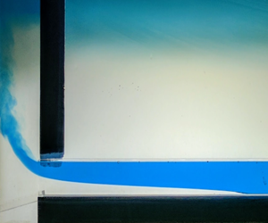
Figure 4. A closeup image of an intruding salt wedge during an experiment. Here, freshwater (dyed blue) is observed exiting the channel as a salt wedge intrudes the lower portion of the channel. The freshwater plume and the diluted mixed layer are visible in the left and upper sections of the image respectively.

Each experiment was video recorded with a digital camera. To highlight the interface between the two layers, the inflowing freshwater was dyed blue and the tank was backlit by a diffuse light source (figure 4). To obtain quantitative data, the video recordings were converted to a series of images sampled at 1 Hz and analysed using custom written Python code. Since the dyed water was almost completely opaque to red light, analysing the images through their red channel provided a sharp contrast between the fresh and saline layers. Scanning each image upwards from the base of the channel, the interface was taken to be wherever the red light intensity fell below 10 % of its maximum value. Given the sharp contrast between the two layers, the results are not sensitive to moderate changes to this threshold value. To obtain estimates of the wedge length, we calculated the distance between the nose of the salt wedge and where $Fr=1$ (i.e. the hydraulic control point). For the sloped channel experiments, this entire process was carried out after rotating each image so that the channel was oriented horizontally within the image frame.

While our theory assumes the hydraulic control point exists at the mouth of the channel, in our experiments we find that this transition point tends to occur 1–2 centimetres inside the channel. This minor discrepancy possibly reflects an important limitation to our shallow layer theory, which is only formally justified for properties varying over horizontal length scales much larger than the thickness of the layer. Additionally, external factors such as the circulation just outside the entrance of the channel may also influence flow properties near the entrance of the channel in ways not accounted for by our theory.

Figure 5. Example evolution of a salt wedge for a horizontal channel experiment immersed in $25~\text{g}~\text{kg}^{-1}$ seawater ($g^{\prime }\approx 0.2~\text{m}~\text{s}^{-2}$). (a) Evolution of the salt wedge interface height following successive step reductions in freshwater flow rate. Each line represents the position of the salt wedge interface at a 5 s interval. The bold lines indicate the final wedge position just before the freshwater volume flux was changed. Note that the axes are not to scale in this plot. (b) Wedge length versus time for the volume fluxes shown in (a). The vertical dashed lines indicate when the freshwater flow rate was abruptly reduced to a new value.

Sample results from an experimental run done with a horizontal channel are illustrated in figure 5. In this case, the freshwater flow rate was step-wise reduced from $17$ to $5~\text{cm}^{3}~\text{s}^{-1}$. The time series of the wedge length illustrates that a near-steady state was achieved before each step change in the flow rate was initiated.

4 Experimental results

4.1 Horizontal channel experiments

Figure 6. Results from all horizontal channel experiments. (a) Relationship between wedge length and freshwater flow rate. Dark circles represent baseline experiments conducted with $33~\text{g}~\text{kg}^{-1}$ seawater (some of which were repeated several times) while coloured squares represent experiments done with diluted seawater. (b) Same as (a) but with the wedge length and freshwater flux reformulated as non-dimensional quantities. Dashed line shows solutions of (2.8), assuming $C_{i}=C_{d}=7/Re$.

Figure 6(a) shows the length of the equilibrated salt wedge versus the freshwater flow rate for all horizontal channel experiments. Consistent with theory, larger freshwater flow rates produced shorter salt wedges. Similarly, when the salinity difference between the two layers was reduced, so did the length of the salt wedge. Both of these follow directly from figure 2, since either change leads to an increase in the freshwater Froude number.

To quantitatively compare these laboratory results with theoretical predictions, it is necessary to evaluate the interfacial and wall drag coefficients. The magnitude of these coefficients is obtained by comparing experimental data with theoretical predictions and finding values for the drag coefficients that produce the best agreement. To simplify the problem, we first reduce the number of unknowns to one by considering three limiting cases: $C_{i}=C_{d}$, $C_{i}=0$ and $C_{d}=0$. Assuming the drag coefficients are constant in each limiting case yields $(\tilde{C}_{i},\tilde{C}_{d})=(1,1)$, $(\tilde{C}_{i},\tilde{C}_{d})=(0,1)$ and $(\tilde{C}_{i},\tilde{C}_{d})=(1,0)$. Next, we recall that by integrating (2.8) over the range of $Fr_{0}$ used in our experiments we may obtain the dimensionless salt wedge length $\ell =L\,C_{0}/H$. Thus, we can derive an empirical estimate for $C_{0}$ by computing a least-squares regression line through the predicted $\ell$ versus observed $L$. The slope of this line is equivalent to $C_{0}/H$, provided the line is forced to pass through the origin.

Carrying out this procedure for each limiting scenario yields values that range from $C_{0}=0.02$ for $\tilde{C}_{i}=\tilde{C}_{d}$ to $C_{0}=0.08$ for $\tilde{C}_{i}=0$ (figure 7a). In each case, the coefficient of determination ($r^{2}$) for each fit is approximately 0.80, which suggests a moderately linear relationship between predicted $\ell$ and observed $L$. However, deviations are noticeably large for shorter wedge lengths, which corresponds to higher Froude numbers and freshwater flow rates. In this parameter range, the theoretical predictions systematically underestimate the observed wedge length. This discrepancy suggests that the drag coefficients may have an inverse relationship with the freshwater flow rate, becoming smaller as the flow rate increases. Such an inverse relationship is not unexpected, since the drag coefficients for laminar flows are known to vary inversely with the Reynolds number, which for these experiments had a maximum value of approximately 785. For the case of single-layer laminar pipe flow, we expect $C_{d}=8/Re$ for $Re<2000$ (Moody Reference Moody1944; Chen Reference Chen1979). (Note that this is often expressed in terms of the Darcy friction factor $f_{D}=64/Re$, where $f_{D}=8\,C_{d}$.) For the two-layer flow in our set-up, the dependence may be slightly different, but we assume the same dependence on $Re$ should apply for both $C_{d}$ and $C_{i}$.

Figure 7. Plots showing theoretical versus experimental wedge lengths assuming $\tilde{C}_{i}=0$ (blue dots), $\tilde{C}_{d}=0$ (orange dots) and $\tilde{C}_{d}=\tilde{C}_{i}$ (green dots). (a) Case where drag coefficients $C_{0}$ are assumed to be constant. (b) Case where drag coefficients $C_{0}=\hat{C_{0}}/Re$ are inversely proportional to the Reynolds number $Re$. Coloured lines represent the linear least-squares fit for their respective data points, assuming no $y$-intercept.

We therefore repeat the previous procedure to determine $C_{0}$, but now taking $C_{0}=\hat{C_{0}}/Re$ and applying the least-squares fit to determine $\hat{C_{0}}$. Using this Reynolds-number-dependent parameterization improves the quality of the best fit line in all three cases (figure 7b). When $C_{i}=C_{d}$, the best agreement ($r^{2}=0.97$) is obtained with

(4.1)$$\begin{eqnarray}C_{i}=C_{d}\approx \frac{7}{Re},\end{eqnarray}$$

which is similar to the drag parameterization for laminar flow in a pipe (Moody Reference Moody1944).

Re-scaling the observed wedge lengths by the Reynolds number and plotting those values against the freshwater Froude number causes all the results from the horizontal channel experiments to collapse onto a single curve (figure 6b). More importantly, we are able to reproduce this observed relationship with our theoretical model. This is demonstrated using predictions for the case where $C_{i}=C_{d}\approx 7/Re$. A similar correspondence between observations and theory is obtained when drag coefficients from the other limiting cases are used (not shown).

Using the Reynolds-number-dependent drag coefficients, we also assess our theory’s ability to reproduce the shape of the salt wedge interface (figure 8). This is illustrated using results from a special set of runs wherein the freshwater flow rate was varied back and forth between $7~\text{cm}^{3}~\text{s}^{-1}$ ($Fr_{0}\approx 0.20$) and 14 $~\text{cm}^{3}~\text{s}^{-1}$ ($Fr_{0}\approx 0.43$). As with the other experiments, the salt wedge was allowed to come to rest before changing the freshwater flow rate. While the three limiting cases of our theory predict similar wedge lengths, the shape of the interface differs slightly in each case, with the no-interfacial-drag limit ($\tilde{C}_{i}=0$) being the most distinct. For the low $Fr_{0}$ runs (red lines in figure 8), the $(\tilde{C}_{i},\tilde{C}_{d})=(1,1)$ and $(\tilde{C}_{i},\tilde{C}_{d})=(1,0)$ limits do a generally better job of capturing the slope and height of the wedge interface compared to the $\tilde{C}_{i}=0$ limit. However, the $\tilde{C}_{i}=0$ limit does better near the mouth of the channel, where the interface becomes very steep. Similarly, we find that the $\tilde{C}_{i}=0$ limit produces the best agreement with observations for the higher $Fr_{0}$ runs, when the intrusions are relatively short. These results suggest that the wall and interfacial-drag forces vary somewhat along the length of the salt wedge, with the former being more prominent near the mouth of the channel. Nevertheless, we find that by using integrated approximations of these forces, as captured by our constant-valued drag coefficients, our theory is still able to approximate the general features of the salt wedge interface. Since our primary goal is to predict the overall length of salt wedge intrusions, these results demonstrate that our current theory is suitable for this task.

The runs summarized in figure 8 were also carried out to verify repeatability and to assess how the progressive freshening of the ambient seawater impacted our results. While the wedge lengths did not change appreciably with each repetition, the shape of the wedge evolved slightly with time. Most notably, the wedge became marginally thinner just downstream of the mouth. This result is consistent with our theory, which predicts a gradual thinning of the salt wedge as $g^{\prime }$ decreases (figure 2a). While it is not immediately obvious why these changes are most noticeable near the mouth of the channel, these results confirm that our main results were not adversely affected by variations in experiment duration.

Figure 8. Comparisons between observed and theoretical wedge shapes. The coloured lines show results from an experiment where the freshwater flow rate was alternated between $7~\text{cm}^{3}~\text{s}^{-1}$ (red) and $14~\text{cm}^{3}~\text{s}^{-1}$ (blue). Lighter lines represent interface shapes at later times in the experiment. Overlain are theoretical wedge shapes obtained by assuming $\tilde{C}_{i}=\tilde{C}_{d}$ (solid black line), $\tilde{C}_{i}=0$ (dashed line) and $\tilde{C}_{d}=0$ (dotted line). In each case, the magnitude of the drag coefficients is given by ${\hat{C}}_{0}/Re$, with ${\hat{C}}_{0}$ assuming the values shown in figure 7(b). To facilitate a more direct comparison with theory, each observed profile has been translated horizontally so that its hydraulic control point (i.e. the location where $Fr=1$) is aligned with the origin. The inset shows the time evolution of the wedge length.

4.2 Sloped channel experiments

Several additional experiments were conducted with the channel tilted so that freshwater and saltwater layers flowed upward and downward under the influence of their own buoyancy, respectively. This effectively enhanced the velocity shear across the salt wedge interface, thereby promoting instabilities and interfacial mixing. To maintain salt wedges that fit within our 1 m long channel, we conducted these sloped channel experiments at relatively high freshwater flow rates with undiluted seawater in the tank.

As predicted by theory, introducing a positive channel tilt increased the length of the salt wedge intrusion (figure 9). However, these predicted wedge lengths are generally longer than observed, with progressively larger over-estimations occurring at steeper slopes. Here, we show the theoretical predictions for the limit where ${\hat{C}}_{i}={\hat{C}}_{d}$ and $C_{0}=7/Re$. As before, similar wedge lengths are obtained using the ${\hat{C}}_{i}=0$ and ${\hat{C}}_{d}=0$ limits (not shown). For a channel tilt of $3.3^{\circ }$, the theory predicts infinite saltwater intrusions even though finite salt wedges were observed. These systematic discrepancies indicate our theory neglects one or more key processes that tend to reduce the extent of saltwater intrusions when the channel is tilted. More specifically, it is likely that our wedge model is underestimating the magnitude of the drag forces experienced by the wedge for positive channel slopes. One hypothesis is that enhanced shear across the interface also leads to enhanced momentum dissipation. This assertion is supported by observations of small amplitude interfacial waves, which were most apparent when the salt wedge was relatively long (i.e. at relatively large slopes and weak freshwater inflow). Even though there was no visible wave breaking or entrainment, the presence of these waves strongly suggests that the effective interfacial drag was larger than anticipated by our wedge model. For similar reasons, enhanced wall drag within the salt layer, which is all-together neglected in our simplified theory, may have contributed to this discrepancy. While the net volume flux within the salt layer is zero, the flow within the layer is non-zero and thus contributes to the velocity shear (circulation within the lower layer was confirmed by inserting dye into the salt layer).

Figure 9. Equilibrium wedge length as in figure 6(b), but including results from the sloped channel experiments. Squares indicate experimental data while solid lines represent theoretical predictions, assuming ${\hat{C}}_{i}={\hat{C}}_{d}$ and $C_{0}=7/Re$. The line for $\unicode[STIX]{x1D703}=3.3^{\circ }$ is not shown since the theory predicts infinite saltwater intrusions for the chosen range of $Fr_{0}$. Dashed lines are like the solid lines but with $C_{0}=8.5/Re$ and $C_{0}=9/Re$ for the $\unicode[STIX]{x1D703}=2.2^{\circ }$ and $\unicode[STIX]{x1D703}=3.3^{\circ }$ cases, respectively.

In summary, the drag coefficients that were obtained using data from the horizontal channel experiments are likely not appropriate for the tilted channel experiments. This hypothesis is supported by the dashed lines in figure 9, which show predicted wedge lengths using slightly larger values for $C_{0}$. By assuming $C_{0}=8.5/Re$ for the $\unicode[STIX]{x1D703}=2.2^{\circ }$ case, we obtain much better agreement with the data. We achieve similar improvement by using $C_{0}=9/Re$ for the $\unicode[STIX]{x1D703}=3.3^{\circ }$ case. However, at this angle, there is still clear discrepancies between the theory and observations, especially at higher Froude numbers. This may indicate that the flow was starting to transition to a regime where the $1/Re$ dependence in the drag coefficients no longer holds.

Tilting the channel at even greater angles and subsequently increasing the freshwater flow rate, led to larger amplitude interfacial waves. At sufficiently steep channel slopes these waves began to overturn, which led to visible mixing between the two layers. At the steepest slopes obtained within the tank ($\unicode[STIX]{x1D703}\approx 8^{\circ }$), the salt wedge interface was unsteady and completely distorted (figure 10). In one experimental run, the freshwater flow rate was held at $28~\text{cm}^{3}~\text{s}^{-1}$ ($Fr\approx 0.86$) for just over 12 min. For the latter portion of this run, the nose of the salt wedge occupied roughly the same position within the channel. During this period, the flow downstream of the salt wedge displayed episodic bursts of interfacial mixing. Such strong mixing episodes clearly violate the no-entrainment assumption used to formulate our theory. Whilst not the primary focus here, these results highlight the need for further theoretical development.

Figure 10. Rotated images showing the time evolution of interfacial waves inside a ‘steeply’ sloped channel. For this experiment, the channel was tilted at approximately $8^{\circ }$ and the freshwater flow rate was set to $28~\text{cm}^{3}~\text{s}^{-1}$ ($Fr\approx 0.86$). In the top image, the blue arrow indicates the direction of the freshwater flow. Yellow vertical lines are added to highlight the evolution of the interface near the nose of the wedge.

5 Discussion: seawater intrusions in a realistic subglacial channel

With these theoretical results, we now assess the likelihood of saltwater intrusions in realistic subglacial channels. This exercise comes with the obvious caveat that our theory has only been compared to laboratory experiments and neglects processes, such as entrainment, that are likely to be more significant at the much larger Reynolds numbers inherent to the geophysical scale (e.g. a discharge $Q=10~\text{m}^{3}~\text{s}^{-1}$, and channel width $W=10~\text{m}$, gives an estimate of $Re=10^{6}$). Nevertheless, we posit that the dynamics that occur at these larger scales are similar to those observed in our laboratory experiments and that the inclusion of processes such as entrainment will refine rather than fundamentally alter our predictions. Although our experimental results suggest that the drag coefficients are inversely proportional to $Re$ in the laminar regime, we do not expect this dependence to hold in the turbulent regime of geophysical flows. We instead assume that these coefficients will asymptote towards constant values with increasing $Re$, as they do in single-layer pipe flows (Moody Reference Moody1944). For turbulent flows along relatively smooth ice, whether along the face of glacier or floating sea ice, theoretical models and observational estimates suggest wall drag coefficient values that range from 0.001–0.01 (e.g. Jenkins Reference Jenkins2011; Lu et al. Reference Lu, Li, Cheng and Leppäranta2011; Werder et al. Reference Werder, Hewitt, Schoof and Flowers2013; Slater et al. Reference Slater, Goldberg, Nienow and Cowton2016; Ezhova, Cenedese & Brandt Reference Ezhova, Cenedese and Brandt2018). Direct estimates for $C_{i}$ are sparse but values of the order of $10^{-4}$ are commonly used in the estuarine literature (e.g. Geyer & Ralston Reference Geyer and Ralston2011). We therefore expect $C_{d}>C_{i}$ within the subglacial channel, which means the length of the salt wedge should scale with the magnitude of $C_{d}$.

Figure 11. Simulations of salt wedge properties for a range of realistic subglacial channels and discharge rate: (a) freshwater Froude number $Fr_{0}=Q/\sqrt{g^{\prime }H^{3}W^{2}}$ and (b) predicted salt wedge lengths assuming $C_{d}=0.005$ and $C_{i}=0.0001$. For these calculations, ambient ocean salinity is assumed to be $33~\text{g}~\text{kg}^{-1}$ ($g^{\prime }=0.26~\text{m}~\text{s}^{-2}$). The channel is assumed to be horizontal with a square cross-section ($H=W$). Grey shading in both plots represents regimes where the freshwater flow is super critical and prohibits the intrusion of salt water. In (a), white contours represent lines of constant Reynolds number.

Assuming a range of realistic subglacial flows ($0<Q\leqslant 100$$~\text{m}^{3}~\text{s}^{-1}$ and $0<H\leqslant 20$ m), our theory predicts that typical subglacial channels can support subcritical flow ($Fr_{0}<1$) for sufficiently large channels or low enough discharge, which permits the intrusion of seawater (figure 11a). Taking $C_{i}=0.0001$ and $C_{d}=0.005$ as representative values and integrating (2.8) over the previously stated range for $Q$ and $H$, we find that these intrusions can be several kilometres long. While this is a crude prediction that neglects many complicating factors, this result suggests that the ocean has a strong tendency to penetrate subglacial channels. Since this tendency is greater for wider channels and weaker discharge, we would expect longer saltwater intrusions in the winter, when the discharge is at a minimum, and possibly no intrusion in the summer when the flow is potentially supercritical. Furthermore, since warm saline water lies below the presumably colder freshwater layer, there is potential for these channels to melt faster along their sides relative to their top. More importantly, such melting will be self-reinforcing as larger channels promote greater intrusion of warm seawater. We therefore hypothesize that the combination of this positive feedback along with the strong reduction in discharge during winter will cause most subglacial outlets to widen over time. This process may be responsible for the formation of line plumes, which are observed along some glaciers (e.g. Fried et al. Reference Fried, Catania, Bartholomaus, Duncan, Davis, Stearns, Nash, Shroyer and Sutherland2015). Given that we have neglected many external factors, we must acknowledge that salt intrusions on the order of kilometres may not necessarily exist in reality. For example, variations in the channel cross-section or slope could severely limit the intrusion of water. We nevertheless maintain that such intrusions could occur and that they would have far-reaching consequences.

6 Summary and conclusion

In this study, we investigated the dynamics of subglacial plume lift-off using a combination of idealized models and laboratory experiments. We developed our theoretical framework with the critical assumption that the flow system near the outlet of a subglacial channel is fundamentally similar to that of a salt wedge estuary. With this understanding, we formulated a theory that describes the steady-state properties of a non-entraining salt wedge confined to a rectangular channel. This theory predicts the shape and length of a salt wedge for a given freshwater volume flux, wedge salinity, channel size and slope. The first three parameters are captured by the non-dimensional freshwater or densimetric Froude number, $Fr_{0}=Q/\sqrt{g^{\prime }H^{3}W^{2}}$. In parallel with this theoretical effort, a series of laboratory experiments were conducted to observe the behaviour of a salt wedge in a rectangular channel. In these experiments, freshwater was pumped through a narrow rectangular channel into the bottom of a tank, filled with water of higher salinity. To simulate flow over a wide range of Froude numbers, these experiments were conducted with various freshwater flow rates and tank salinities. Additional experiments were carried out with the channel tilted so that the freshwater flowed upward with the additional assistance of its own buoyancy.

In general, we find good qualitative agreement between the theoretical predictions and laboratory results. Consistent with theory, increasing the freshwater Froude number, either by increasing the freshwater volume flux or reducing the salinity of the salt wedge, led to shorter salt wedges while tilting the mouth of the channel upwards led to longer intrusions. Appropriate values for the wall and interfacial drag coefficients were determined by applying a least-squares fit to the experimental data. For cases where the channel was horizontal and showed no signs of interfacial mixing, assuming $C_{d}=C_{i}\approx 7/Re$ produces good agreement between theoretical and observed wedge lengths ($r^{2}\approx 0.97$). Similar agreement can be attained by considering the theoretical limits where $C_{d}=0$ or $C_{i}=0$. The theory is also able to accurately reproduce the observed shape of the salt wedge interface when the channel is horizontal. However, a careful comparison between the theory and observations suggest that the drag coefficients may vary along the length of the salt wedge. An interesting challenge for future work is determining and quantifying the factors controlling the variation of the drag coefficients along the length of the flow. Nevertheless, the good agreement between observed and predicted wedge lengths suggests the present theory adequately approximates the key dynamics controlling salt wedge lengths

Applying the parameterizations for the drag coefficients obtained from the horizontal channel experiments to experiments with small positive channel slopes ($\unicode[STIX]{x1D703}\lesssim 3.5^{\circ }$) yielded relatively poor quantitative agreement with theoretical predictions. We suspect that this discrepancy is in large part due to an underestimation of the drag forces acting on the salt wedge when the channel slope is tilted. In support of this hypothesis, we obtain better agreement with observations when we assume slightly larger values for the drag coefficients with sloping channels. For channel slopes as small as ${\sim}2^{\circ }$, we observed small amplitude internal waves propagating along the salt wedge interface. At progressively steeper slopes, these interfacial waves grew and eventually became unstable, leading to episodic mixing between the two layers. These observations demonstrate the need for a more general, time-dependent salt wedge model that permits the exchange of mass and momentum across the wedge interface.

Given that the flow within realistic subglacial channels is fully turbulent, application of our theory to this setting must be done with some caution. Specifically, there is still considerable uncertainty regarding the magnitude of the drag coefficients at higher Reynolds numbers, when entrainment is substantial. Nevertheless, much like the case of a salt wedge in coastal estuaries, these highly turbulent subglacial flows should still be governed by the fundamental dynamics described by our theory. Moreover, we posit that the enhanced mixing and momentum transfer associated with interfacial mixing can still be captured by an appropriate parameterization for the interfacial drag. These drag coefficients are also not expected to share the same dependence on $Re$ as is the case for laminar flows. Assuming reasonable values for the drag coefficients ($C_{d}=0.005$ and $C_{i}=0.0001$), the theoretical model predicts that typical subglacial channels may permit salt wedge intrusions as long as several kilometres, depending on the channel size and discharge rate. While necessarily crude, this result suggests that the ocean has a strong tendency to penetrate and potentially widen existing subglacial channels. This mechanism may be responsible for the line plumes of subglacial discharge observed along tidewater glaciers in Greenland (Fried et al. Reference Fried, Catania, Bartholomaus, Duncan, Davis, Stearns, Nash, Shroyer and Sutherland2015; Jackson et al. Reference Jackson, Shroyer, Nash, Sutherland, Carroll, Fried, Catania, Bartholomaus and Stearns2017).

A natural extension of our current work would be to develop a salt wedge theory that explicitly accounts for entrainment. A good starting point would be the model presented by Arita & Jirka (Reference Arita and Jirka1987a), which accounts for entrainment and momentum transfer between the two layers. This effort would ideally be done in conjunction with laboratory experiments that generate fully turbulent flows. While such experiments would almost certainly require a larger experimental set-up, doing so would allow for proper determination of the drag and entrainment coefficients. Another interesting extension would be to consider the additional mixing that may arise due to nonlinearities in the equation of state. Given the temperature and salinity ranges observed in glacial settings and the vertical configuration of cold, fresh water over relatively warm, salty water, we might anticipate the potential for double diffusive convective instability across the density interface, in addition to shear-driven mixing.