


1. Introduction
A hallmark feature of three-dimensional (3-D) turbulence is the forward energy cascade, transporting kinetic energy from large scales to ever smaller scales, as described by the celebrated theory of Kolmogorov (Reference Kolmogorov1941). In many geophysical and astrophysical flows, however, velocity fluctuations are largely suppressed in one direction as a consequence of, for example, confinement (Benavides & Alexakis Reference Benavides and Alexakis2017; Musacchio & Boffetta Reference Musacchio and Boffetta2017, Reference Musacchio and Boffetta2019), strong magnetic fields (Alexakis Reference Alexakis2011; Seshasayanan, Benavides & Alexakis Reference Seshasayanan, Benavides and Alexakis2014) or fast rotation (Smith, Chasnov & Waleffe Reference Smith, Chasnov and Waleffe1996; Seshasayanan & Alexakis Reference Seshasayanan and Alexakis2018; Pestana & Hickel Reference Pestana and Hickel2019; van Kan & Alexakis Reference van Kan and Alexakis2020), rendering the flow quasi-two-dimensional. This leads to the development of an inverse energy flux, akin to fully 2-D turbulence (Kraichnan Reference Kraichnan1967; Batchelor Reference Batchelor1969), transporting energy from smaller to larger scales. Ultimately, this can lead to accumulation of kinetic energy at the largest available scales, followed by condensation into a vertically coherent large-scale vortex (LSV) structure at the domain size (see Alexakis & Biferale (Reference Alexakis and Biferale2018) for a recent review). These LSVs are believed to play a crucial role in, for example, the formation of the Earth's magnetic field (Roberts & King Reference Roberts and King2013; Aurnou et al. Reference Aurnou, Calkins, Cheng, Julien, King, Nieves, Soderlund and Stellmach2015; Guervilly, Hughes & Jones Reference Guervilly, Hughes and Jones2015).
Following the framework that is brought forward in Alexakis & Biferale (Reference Alexakis and Biferale2018), we aim to classify the transition from a 3-D forward cascading state to the condensate state by considering the behaviour of an order parameter that measures the strength of the LSV as a function of a control parameter of the flow throughout this transition. Then one can observe either a smooth transition, a continuous transition with discontinuous derivative or a discontinuous transition. This categorisation of the transition into the condensate state has shown to be an insightful approach in various other quasi-2-D flow systems (Alexakis Reference Alexakis2015; Yokoyama & Takaoka Reference Yokoyama and Takaoka2017; Seshasayanan & Alexakis Reference Seshasayanan and Alexakis2018; van Kan & Alexakis Reference van Kan and Alexakis2019).
These earlier works, however, have focused on more artificial, idealised flow models, where the turbulent forcing occurs at a single well-defined length scale. Here, we characterise the LSV transition in a natural, broadband-forced system of rotating convection, which is ubiquitous in geophysical and astrophysical flows. In this system, Favier, Guervilly & Knobloch (Reference Favier, Guervilly and Knobloch2019) have shown a bistability of an LSV with a non-LSV state at the same parameter values, depending on the initial conditions. The natural buoyant forcing over a broad range of scales obfuscates the strict separation of the injection, dissipation and condensation scales. Although one may expect that, in such natural and vigorously fluctuating turbulent systems, any transitions between different states are washed out and become gradual, we find that the transition towards the condensate state is in fact sharp and discontinuous.
Such abrupt transitions between turbulent states in a more general sense are a remarkable feature of fluid turbulence and have received much recent interest, being observed in various different flow settings, e.g. in torque measurements of Taylor–Couette and Von Kármán flows (Ravelet et al. Reference Ravelet, Marié, Chiffaudel and Daviaud2004; Saint-Michel et al. Reference Saint-Michel, Dubrulle, Marié, Ravelet and Daviaud2013; Huisman et al. Reference Huisman, van der Veen, Sun and Lohse2014), in states of stochastically forced 2-D and 3-D turbulence (Bouchet & Simonnet Reference Bouchet and Simonnet2009; Iyer et al. Reference Iyer, Bonaccorso, Biferale and Toschi2017; Bouchet, Rolland & Simonnet Reference Bouchet, Rolland and Simonnet2019) and in reversals of the large-scale dynamics in thin layers (Sommeria Reference Sommeria1986; Michel et al. Reference Michel, Herault, Pétrélis and Fauve2016; Dallas, Seshasayanan & Fauve Reference Dallas, Seshasayanan and Fauve2020). These types of abrupt transition are surmised to play an important role in, for example, climate research (Weeks et al. Reference Weeks, Tian, Urbach, Ide, Swinney and Ghil1997; Jackson & Wood Reference Jackson and Wood2018; Herbert, Caballero & Bouchet Reference Herbert, Caballero and Bouchet2020) and in understanding the geomagnetic reversal (Berhanu et al. Reference Berhanu2007; Pétrélis et al. Reference Pétrélis, Fauve, Dormy and Valet2009).
2. Numerical approach
We consider the canonical system of rotating Rayleigh–Bénard convection, in which the flow is driven by buoyancy through a temperature difference  $\Delta T$ between the bottom and top of the domain, whilst being simultaneously affected by strong background rotation $\varOmega$ along the vertical axis. The input space to this problem is described by three dimensionless numbers: the Rayleigh number $Ra=g\alpha \Delta T H^3/(\nu \kappa )$, quantifying the strength of the thermal forcing, the Ekman number ${Ek}=\nu /(2\varOmega H^2)$, representing the (inverse) strength of rotation, and the Prandtl number $Pr=\nu /\kappa$, containing the diffusive properties of the fluid. Here, $g$ denotes gravitational acceleration, $H$ is the domain height and $\alpha$, $\nu$ and $\kappa$ represent the thermal expansion coefficient, kinematic viscosity and thermal diffusivity of the fluid, respectively. The system is non-dimensionalised into convective units using $H$,
$H$,  $\Delta T$ and the free-fall velocity $U=\sqrt {g\alpha \Delta T H}$.
We solve the full governing set of Boussinesq Navier–Stokes equations through direct numerical simulation, employing the finite-difference code described in Verzicco & Orlandi (Reference Verzicco and Orlandi1996) and Ostilla-Monico et al. (Reference Ostilla-Monico, Yang, van der Poel, Lohse and Verzicco2015) on a Cartesian grid with periodic sidewalls and stress-free boundary conditions at the top and bottom. For the width  $D$ of the domain, we choose $D/H=10\mathcal {L}_c$ with $\mathcal {L}_c=4.8{Ek}^{1/3}$ the most unstable wavelength at onset of convection (Chandrasekhar Reference Chandrasekhar1961). The complete set of input parameters as well as the employed resolutions are provided in table 1. Note that we include the convective Rossby number $Ro=U/(2\varOmega H)={Ek}\sqrt {Ra/Pr}$ for reference. A validation of the grid resolution is provided in Appendix A.
Table 1. The different series of input parameters used in this work.

For numerical convenience, we use  $Pr=1$ and ${Ek}=10^{-4}$, for which stable LSVs have been observed in earlier direct numerical simulations over a limited range of $Ra$ (Favier, Silvers & Proctor Reference Favier, Silvers and Proctor2014; Guervilly, Hughes & Jones Reference Guervilly, Hughes and Jones2014; Favier et al. Reference Favier, Guervilly and Knobloch2019). Upon increasing $Ra$ from the onset of convection, the two boundaries of the region of existence of the LSV are crossed. At the low- $Ra$ transition, the LSV develops as sufficient turbulent forcing is obtained to set up the upscale transport into the condensate, whereas at the high- $Ra$ transition, the LSV breaks down as too strong thermal forcing renders the flow insufficiently rotationally constrained, breaking the quasi-2-D conditions for upscale energy flux (Favier et al. Reference Favier, Silvers and Proctor2014; Guervilly et al. Reference Guervilly, Hughes and Jones2014). We carry out a total of 46 runs at varying $Ra$, concentrated around both LSV transitions.
In order to analyse the LSV, we decompose the flow field  $\boldsymbol {u}=u\boldsymbol {e}_x+v\boldsymbol {e}_y+w\boldsymbol {e}_z$ into a 2-D (vertically averaged) barotropic flow and a 3-D (depth-dependent) baroclinic flow (following Julien et al. Reference Julien, Rubio, Grooms and Knobloch2012; Favier et al. Reference Favier, Silvers and Proctor2014, Reference Favier, Guervilly and Knobloch2019; Rubio et al. Reference Rubio, Julien, Knobloch and Weiss2014; Aguirre Guzmán et al. Reference Aguirre Guzmán, Madonia, Cheng, Ostilla-Mónico, Clercx and Kunnen2020; Maffei et al. Reference Maffei, Krouss, Julien and Calkins2021), i.e. $\boldsymbol {u}=\boldsymbol {u}^{2D}+\boldsymbol {u}^{3D}$, where
 \begin{equation} \boldsymbol{u}^{2D}=\overline{u}\boldsymbol{e}_x+\overline{v}\boldsymbol{e}_y,\quad \boldsymbol{u}^{3D}=\underbrace{(u-\overline{u})}_{u'}\boldsymbol{e}_x +\underbrace{(v-\overline{v})}_{v'}\boldsymbol{e}_y+w\boldsymbol{e}_z, \end{equation}
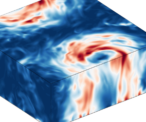
where the overbar  $\overline {{\cdots }}$ denotes vertical averaging. Since the LSV is a largely vertically coherent structure (see figure 1), it resides primarily in the 2-D field, whereas the turbulent baroclinic fluctuations are captured by the 3-D field. Accordingly, we decompose the total kinetic energy $E_{tot}=\tfrac {1}{2}\langle |\boldsymbol {u}|^2\rangle$ into 2-D and (horizontal and vertical) 3-D contributions $E_{tot}=E^{2D}+E_H^{3D}+E_V^{3D}$ as
 \begin{equation} E^{2D}=\tfrac{1}{2}\langle\overline{u}^2+\overline{v}^2\rangle,\quad E_H^{3D}=\tfrac{1}{2}\langle u'^2+v'^2\rangle,\quad E_V^{3D}=\tfrac{1}{2}\langle w^2\rangle, \end{equation}
where angular brackets  $\langle \cdots \rangle$ represent an average over the full spatial domain. We also consider the energy spectrum of the 2-D flow from its Fourier transform $\hat {\boldsymbol {u}}^{2D}_{k_x k_y}$ as
 \begin{equation} \hat{E}^{2D}(K)=\sum_{K\leq\sqrt{k_x^2+k_y^2}< K+1} \frac{1}{2}|\hat{\boldsymbol{u}}^{2D}_{k_x k_y}|^2, \end{equation}
where we normalise the wavenumber  $K$ by the box-size mode $2{\rm \pi} /D$, such that the LSV occupies the $K=1$ mode of the spectrum.

Figure 1. Snapshot of horizontal kinetic energy (in units of  $U^2$) of the LSV-forming case $Ra=1.7\times 10^7$, truncated at three-quarter height to reveal a cross-section of the LSV.
3. Results and discussion
In figure 2, the different components of kinetic energy are provided over the range of considered  $Ra$, crossing both LSV transitions. From the (largest mode of) 2-D energy that captures the LSV, we find a substantial discontinuity at both boundaries of the LSV state. At the high- $Ra$ transition, we find that this transition is hysteretic: the morphology of the flow depends on its history i.e. its initial conditions. These findings are in line with Favier et al. (Reference Favier, Guervilly and Knobloch2019), showing this bistability of an LSV and a non-LSV state for one case in this parameter range. To study this hysteresis loop, we initialise simulations using flow snapshots from a preceding $Ra$. For decreasing $Ra$ from a non-LSV state, the lower branch of the hysteresis loop is followed (open diamonds), whilst for increasing $Ra$ from an LSV state, the flow adheres to the upper hysteretic branch (filled squares), see figure 2. Note the remarkably large discontinuity in the lower hysteretic branch, where the flow transitions directly from a non-LSV state into nearly the strongest LSV forming state. Hysteresis in the LSV transition has also been observed in a rotating flow system with a sharp bandwidth Taylor–Green forcing (Yokoyama & Takaoka Reference Yokoyama and Takaoka2017).

Figure 2. Averaged kinetic energy components as a function of  $Ra$. Filled squares: upper hysteretic branch of the high- $Ra$ transition; open diamonds: lower hysteretic branch. The cyan dashed-dotted line denotes the low- $Ra$ LSV transition, whilst the magenta and red lines denote the LSV transition of the lower and upper branch of the high- $Ra$ transition, respectively.
At the low- $Ra$ transition, on the other hand, no hysteresis is observed (using increments in $Ra$ of $\sim$2 %). Considering the cases directly above the LSV transition, however, we find that the growth of the LSV from a non-LSV state is non-monotonic: the flow shows an evident plateau during which the LSV has not yet developed, before finally growing relatively suddenly into the stable LSV state, see figure 3(a). The flow in this plateau state shows morphological similarities to the jet state observed in rectangular domains (Guervilly & Hughes Reference Guervilly and Hughes2017; Julien, Knobloch & Plumley Reference Julien, Knobloch and Plumley2018), but alternates between being predominantly in the $x$- and $y$-direction. We hypothesise that the peculiar growth behaviour found here signifies a memoryless abrupt growth process, much akin to the nucleation and growth type of dynamics that is observed in plentiful different systems throughout physics (Matsumoto, Saito & Ohmine Reference Matsumoto, Saito and Ohmine2002; Watanabe, Suzuki & Ito Reference Watanabe, Suzuki and Ito2010; Garmann, Goldfain & Manoharan Reference Garmann, Goldfain and Manoharan2019; Metaxas et al. Reference Metaxas, Lim, Booth, Zhen, Stanwix, Johns, Aman, Haandrikman, Crosby and May2019). To substantiate this conjecture, we simulate an ensemble of 100 additional runs at $Ra=6\times 10^6$ with statistically perturbed initial conditions, using a reduced resolution of $128\times 128\times 72$ for computational feasibility. The hypothesised abrupt memoryless growth would then predict an exponential distribution of the waiting time spent in the metastable plateau state (stage B in figure 3a).

Figure 3. (a) Time evolution of horizontal kinetic energy of seven of the runs in the ensemble of the LSV-forming case  $Ra=6\times 10^6$ close to the transition. We distinguish four stages: an initialisation phase (A), a metastable underdeveloped plateau state showing alternating jets (B), (quick) growth of the LSV (C) and the stably developed LSV state (D). The horizontal dashed line denotes the threshold to be crossed and sustained for 2000 convective time units ( $U^{-1}H$) before the LSV is said to be completely developed, which defines the time point $t_{LSV}$, depicted by the blue cross. (b) Cumulative distribution of $t_{LSV}$ of the ensemble (blue solid line) with 95 % confidence bounds (blue dotted lines). It is fitted by an exponential distribution (red dashed line) as provided by (3.1). Inset shows the histogram corresponding to the same distribution.
To investigate the distribution of these waiting times, we define a time point  $t_{LSV}$ at which the LSV is said to have stably developed once a threshold of horizontal kinetic energy is surpassed and sustained for 2000 convective time units, see figure 3(a). The obtained empirical cumulative distribution is then fitted with an exponential distribution
 \begin{equation} CDF(t_{LSV})=1-\exp\left(-\frac{t_{LSV}-t_0}{\underbrace{\mu(t_{LSV})-t_0}_{\tau_W}}\right), \end{equation}
where the fit parameter  $t_0$ can be interpreted as the (fixed) contributions of the initialisation, growth and stable LSV stages (A, C and D in figure 3a). Here, $\mu (t_{LSV})$ denotes the mean of $t_{LSV}$, providing the maximum-likelihood estimate for the typical waiting time $\tau _W$ in this distribution. Figure 3(b) shows that there is excellent agreement between the hypothesised and the obtained distributions: the exponential distribution remains everywhere in between the 95 % confidence bounds of the empirical distribution. Signs of the exponentiality of waiting times have been observed in the LSV-forming system of sharp bandwidth forced thin-layer turbulence (van Kan, Nemoto & Alexakis Reference van Kan, Nemoto and Alexakis2019). Our findings indicate that, indeed, turbulent fluctuations randomly trigger the growth of the LSV, giving rise to this memoryless abrupt growth dynamics. Similar sudden growth behaviour is also found near the ends of the hysteresis loop in the high- $Ra$ transition, although an extended analysis of how the mean transition time evolves for changing $Ra$, repeating the ensemble average approach for all points in the considered parameter space, is currently out of computational reach for rotating convection.
Considering the observed hysteretic behaviour as well as the exponentially distributed waiting times, an analogy of this transition with first-order phase transitions in equilibrium statistical mechanics seems appropriate (Binder Reference Binder1987). However, although it is conjectured that in particular the relatively more weakly dissipative large scales of the flow may show resemblance to thermal equilibrium states (Bouchet & Venaille Reference Bouchet and Venaille2012; Alexakis & Biferale Reference Alexakis and Biferale2018), ultimately, the chaotic and dissipative nature of turbulence makes the analogy with equilibrium statistical mechanics indirect. A more immediate interpretation of the transition in this fluctuating dynamical system would be in terms of nonlinear bifurcations. Then, the condensate transition as observed here can be interpreted as a subcritical nonlinear bifurcation, giving rise to two distinct attractors (indeed, the LSV state and the non-LSV state) which remain separated in phase space. Such noise-induced transitions between attractors are also known to be memoryless, yielding exponentially distributed waiting times (Kraut, Feudel & Grebogi Reference Kraut, Feudel and Grebogi1999).
To understand how the LSV is energetically sustained, we compute the mode-to-mode kinetic energy transfer (see Dar, Verma & Eswaran Reference Dar, Verma and Eswaran2001; Alexakis, Mininni & Pouquet Reference Alexakis, Mininni and Pouquet2005; Mininni, Alexakis & Pouquet Reference Mininni, Alexakis and Pouquet2005, Reference Mininni, Alexakis and Pouquet2009; Verma, Kumar & Pandey Reference Verma, Kumar and Pandey2017; Verma Reference Verma2019), distinguishing the 3-D to 2-D (baroclinic to barotropic) transport (following Rubio et al. Reference Rubio, Julien, Knobloch and Weiss2014; Aguirre Guzmán et al. Reference Aguirre Guzmán, Madonia, Cheng, Ostilla-Mónico, Clercx and Kunnen2020)
 \begin{equation} T_{3D}(K,Q)={-}\langle\boldsymbol{u}^{2D}_K\boldsymbol{\cdot}(\overline{\boldsymbol{u}^{3D} \boldsymbol{\cdot} \boldsymbol{\nabla} \boldsymbol{u}^{3D}_Q})\rangle, \end{equation}
and the 2-D to 2-D (barotropic to barotropic) transport
 \begin{equation} T_{2D}(K,Q)={-}\langle\boldsymbol{u}^{2D}_K\boldsymbol{\cdot} (\boldsymbol{u}^{2D}\boldsymbol{\cdot}\boldsymbol{\nabla} \boldsymbol{u}^{2D}_Q)\rangle, \end{equation}
describing the energetic transport into the Fourier-filtered 2-D flow field  $\boldsymbol {u}^{2D}_K$ of mode $K$ from 3-D and 2-D modes $Q$ through triadic interactions arising from the advective term of Navier–Stokes. If $T_{3D},T_{2D} > 0$, there is a net transfer of kinetic energy from mode $Q$ to mode $K$ and vice versa. We also consider the transport into 3-D mode $K$ from the full (unfiltered) flow components $\mathcal {T}_{3D}(K)=\sum _Q T_{3D}(K,Q)$ and $\mathcal {T}_{2D}(K)=\sum _Q T_{2D}(K,Q)$, by summing over the donating modes $Q$.
$Q$.
The results for the shell-to-shell energy transfer throughout the LSV transitions are provided in figure 4. The two main energy fluxes are apparent in both  $T_{3D}$ and $T_{2D}$. Near the diagonal, one can observe the direct forward cascade, transporting energy from $Q$ to slightly higher modes $K$. Note here that, while the $T_{2D}$ self-interaction must be symmetric by definition $T_{2D}(K,Q)=-T_{2D}(Q,K)$, this does not apply to $T_{3D}$ as it describes the energetic interactions between scales of the 2-D component and 3-D component of the flow. In the bottom row $K=1$, on the other hand, the upscale energy flux into the LSV can be appreciated. This energy flux is non-local: energy is transported directly from virtually all scales in the system into the box scale of the LSV, without participation of intermediate scales.

Figure 4. Time-averaged kinetic energy transport from 3-D (a,c,e,g) or 2-D (b,d, f,h) modes  $Q$ to 2-D modes $K$, i.e. $T_{3D}(K,Q)$ and $T_{2D}(K,Q)$, respectively, in units of $U^3H^{-1}$. Blue lines denote $\mathcal {T}_{3D}(K)$ (a,c,e,g) and $\mathcal {T}_{2D}(K)$ (b,d, f,h). The low- $Ra$ transition is crossed from (a,b) ( $Ra=5.6\times 10^6$) to (c,d) ( $Ra=5.7\times 10^6$), whilst the high- $Ra$ transition of the upper hysteretic branch is crossed from (e, f) ( $Ra=3.10\times 10^7$) to (g,h) ( $Ra=3.13\times 10^7$), as also depicted in figure 5.
Figure 5 shows the energetic transport into the box-size mode as a function of  $Ra$. Note that this considers the transport from the full, unfiltered 3-D and 2-D flow components into the LSV, that is, a sum over the donating scales in the bottom row $K=1$ of the transfer maps in figure 4. It makes clear that also the upscale transport into the LSV exhibits an evident discontinuous transition, both in $\mathcal {T}_{3D}(K=1)$ as well as, albeit to a lesser degree, in $\mathcal {T}_{2D}(K=1)$. Importantly, the figure indicates that it is the 3-D transport that is the dominant component in the forcing of the LSV.


We argue that this upscale transport provides a clue to understanding the physical mechanism behind the observed sudden growth and hysteretic behaviour. As also detailed in Rubio et al. (Reference Rubio, Julien, Knobloch and Weiss2014) and Favier et al. (Reference Favier, Guervilly and Knobloch2019), the upscale transport contains a positive feedback loop, where the presence of the LSV itself enhances the upscale transport into the box-size mode. This agrees with our observation that the energetic transport into the LSV increases discontinuously as the LSV is created. The exact nature of how the LSV interacts energetically with its 3-D turbulent background is an interesting non-trivial question to explore in future work, which goes beyond considerations purely in Fourier space as well, by looking at individual vortex interactions, for example. The existence of such a positive feedback loop, however, seems intuitive: the predominantly cyclonic LSV locally increases the total vorticity (background rotation + flow vorticity), thereby strengthening the quasi-2-D conditions and hence the upscale transport. This mechanism allows the LSV to develop once its growth is triggered by rare turbulent fluctuations and allows the LSV to remain stably self-sustained over the hysteresis loop.
Since we consider specifically a cross-section of the full parameter space for varying  $Ra$, the influence of other parameters on the transitional dynamics, such as ${Ek}$, $Pr$ and also the aspect ratio $D/H$ (since the domain width is the principal dynamical scale of the LSV), remains an open question. The morphology of the LSV in the asymptotically reduced model for ${Ek}\to 0$ is studied in its total parameter space in more detail in Maffei et al. (Reference Maffei, Krouss, Julien and Calkins2021). For the transition specifically, however, one can argue that, as both attractors are expected to shift in continuous fashion through the phase space, only quantitative changes to the observed transitional dynamics are expected as the other control parameters are varied in vicinity to the computationally tractable values considered here. Nonetheless, the possibility that the discontinuity in the transition vanishes in a certain limit if both attractors would shift to coincide cannot be ruled out from the current simulations; the asymptotically reduced model seems appropriate to investigate this premise for the limit ${Ek}\to 0$.
4. Conclusions
We have described the fluid turbulence transition into a quasi-2-D condensate state in a natural broadband-forced system of rotating Rayleigh–Bénard convection, where the transition is sharply discontinuous, in spite of the lack of a clear separation of scales. We provide evidence of memoryless abrupt growth dynamics and hysteresis in these transitions, raising the picture of a double attractor phase space with a subcritical noise-induced transition between them. Furthermore, the correspondence of our findings with certain aspects of the LSV transition in other, artificially forced, flow systems, as remarked in the text, ultimately shows that this peculiar type of transition is a relevant and robust phenomenon that is expected to survive even in the geo- and astrophysically relevant flow of rotating convection, being one of the principal sources of fluid motion in nature.
Acknowledgements
We thank W.G. Ellenbroek for careful reading of the manuscript.
Funding
A.J.A.G. and R.P.J.K. received funding from the European Research Council (ERC) under the European Union's Horizon 2020 research and innovation programme (Grant Agreement No. 678634). We are grateful for the support of the Netherlands Organisation for Scientific Research (NWO) for the use of supercomputer facilities (Cartesius) under Grants No. 2019.005 and No. 2020.009.
Declaration of interests
The authors report no conflict of interest.
Appendix A. Grid validation
We employ a Cartesian grid that is uniform in the  $x$- and $y$-directions, but non-uniform in the $z$-direction, clustering grid cells more closely near the top and bottom of the domain to properly resolve the boundary layers.
The different spatial resolutions that are used in this work are included in table 1 of the main text. To validate these resolutions, we separately consider the bulk flow and the boundary layers. For the bulk resolution, we compare the grid spacing with the Kolmogorov length  $\eta$ for the smallest kinematic features, and the Batchelor length $\eta _T$ for the smallest thermal features of the flow. Their respective definitions (Monin & Yaglom Reference Monin and Yaglom1975) can be rewritten into convective units (using the free-fall velocity scale $U$ and length scale $H$) as
 \begin{equation} \tilde{\eta}=\left(\frac{Pr}{Ra}\right)^{3/8}\tilde{\epsilon}^{{-}1/4},\quad \tilde{\eta}_T=\tilde{\eta}Pr^{{-}1/2}, \end{equation}
where  $\tilde {\epsilon }$ denotes the kinetic energy dissipation rate
 \begin{equation} \tilde{\epsilon}=\sqrt{\frac{Pr}{Ra}}|\tilde{\boldsymbol{\nabla}} \tilde{\boldsymbol{u}}|^2. \end{equation}
In our work  $Pr=1$, so that the Batchelor length and Kolmogorov length coincide $\eta =\eta _T$. We can compare the Kolmogorov length with the local grid spacing $\underline {\varDelta }=(\Delta x, \Delta y, \Delta z)$ in each dimension from a posteriori horizontal and temporal averages of the kinetic dissipation. We calculate the number of Kolmogorov lengths per cell in each direction $\underline {\varDelta }/\eta$, as is shown in the example in figure 6(a). (Note that the grid is uniform in the horizontal direction, so we have $\Delta x /\eta = \Delta y /\eta$.) In all simulations, we ensure that we maintain $\underline {\varDelta }/\eta <2$ over the entire vertical extent of the domain, which is well below the limit of $\underline {\varDelta }/\eta <4$ that was empirically found to be acceptable by Verzicco & Camussi (Reference Verzicco and Camussi2003). Also for the ensemble of runs, where we use a coarser grid for computational feasibility (see table 1), we can adhere to $\underline {\varDelta }/\eta <2$ throughout the full domain, owing the moderate $Ra=6\times 10^6$.

Figure 6. Number of Kolmogorov scales per cell (a) and temperature profiles (b) for the example case  $Ra=10^7$ (and ${Ek}=10^{-4}$, $Pr=1$). In (b), the dashed lines indicate the boundary layer edges based on the maximum of the root-mean-squared temperature.
To properly resolve the boundary layers at the top and bottom, we require that a sufficient number of grid cells reside within these boundary layers. Since this work uses stress-free boundary conditions for velocity, there is no formation of any kinematic boundary layers. For the thermal boundary layer, on the other hand, we adopt the definition of maximum (horizontally and temporally averaged) root-mean-squared temperature (e.g. Julien et al. Reference Julien, Rubio, Grooms and Knobloch2012), see figure 6(b). We ensure that there are at least 10 grid cells within the thermal boundary layer for all simulations, which is also empirically deemed sufficient by Verzicco & Camussi (Reference Verzicco and Camussi2003).


 Open access