


1 Introduction
A spherical droplet that comes in contact with a solid substrate will change its shape in order to minimize its total surface energy by generating a spreading motion. Droplet spreading on flat substrates has been widely studied and is quite well understood (Tanner Reference Tanner1979; Hocking Reference Hocking1983; Cox Reference Cox1986; Chen & Wada Reference Chen and Wada1989; Brenner & Bertozzi Reference Brenner and Bertozzi1993; Bonn et al. Reference Bonn, Eggers, Indekeu, Meunier and Rolley2009; Carlson, Bellani & Amberg Reference Carlson, Bellani and Amberg2012). If the flat substrate has a constant equilibrium contact angle, the centre of mass of the droplet will not change its position along the substrate. One way to generate a directional droplet spreading is to manipulate the chemical composition or the microscale/nanoscale structure of the substrate to make the equilibrium contact angle vary on the substrate (Brochard Reference Brochard1989; Chaudhury & Whitesides Reference Chaudhury and Whitesides1992; Dos Santos & Ondarçuhu Reference Dos Santos and Ondarçuhu1995; Sumino et al. Reference Sumino, Kitahata, Yoshikawa, Nagayama, Nomura, Magome and Mori2005; Moosavi & Mohammadi Reference Moosavi and Mohammadi2011; Li et al. Reference Li, He, Zhang, Zhang and Tian2017), where the contact angle difference at the front and back of the droplet generates its motion. An alternative to surface coatings is to instead change the macroscopic shape of the substrate to a geometric structure that breaks the front/rear symmetry, e.g. a cone-like structure. A droplet placed on a fibre with the shape of a cone spontaneously starts to move in the direction of a growing cone radius when the flow is dominated by capillary forces (Bico & Quéré Reference Bico and Quéré2002; Lorenceau & Quéré Reference Lorenceau and Quéré2004). In fact, the principle of capillary induced self-propelled droplets by tuning the macroscopic geometry of the substrate has been widely exploited by living creatures, where plants (Liu et al. Reference Liu, Xue, Chen and Zheng2015) and animals (Zheng et al. Reference Zheng, Bai, Huang, Tian, Nie, Zhao, Zhai and Jiang2010; Duprat et al. Reference Duprat, Bebee, Protiere and Stone2012; Wang et al. Reference Wang, Yao, Liu, Quéré and Jiang2015) have evolved thin structures that generate droplet motion. Cacti that reside in arid regions have developed conical spines for water collection from humid air, which also transport the water droplets from the spine tip to its base for adsorption (Liu et al. Reference Liu, Xue, Chen and Zheng2015). Zheng et al. (Reference Zheng, Bai, Huang, Tian, Nie, Zhao, Zhai and Jiang2010) showed that a similar principle of directional water collection appears on wetted spider silk, where small water droplets condense at the thinner part (the joint) and move to the centre of the thicker part (knots) where multiple droplets in time coalescence to create a large droplet. It was recently shown by Chen et al. (Reference Chen, Ran, Gan, Zhou, Zhang, Zhang, Zhang and Jiang2018b) that the plant Sarracenia trichome has developed a solution for droplet transport that generates velocities three orders of magnitude larger than that found on the spines of cacti by careful design of its macroscopic geometry and its microscopic structure. The biological transport solution in Sarracenia trichome was mimicked in microchannels as a solution for rapid droplet transport. Insects, on the other hand, are in general interested in getting rid of the unwanted weight of water droplets. Water striders have legs covered with tilted conical setae, which are elastic and hydrophobic, and aid the removal of water droplets (Wang et al. Reference Wang, Yao, Liu, Quéré and Jiang2015). Controlled droplet motion has a broad industrial relevance for manipulation of chemical reactions, fabrication of materials that can maintain a dry or a wet state or new materials for water harvesting, where recent advances have found inspiration in nature (Park et al. Reference Park, Kim, Grinthal, He, Fox, Weaver and Aizenberg2016; Chen et al. Reference Chen, Li, Zhao, Guo, Zhang, Sherazi, Ambreen and Li2018a,Reference Chen, Ran, Gan, Zhou, Zhang, Zhang, Zhang and Jiangb).
When the droplet size,  $V^{1/3}$ with $V$ the droplet volume, is smaller than the capillary length $\equiv (\unicode[STIX]{x1D6FE}/\unicode[STIX]{x1D70C}g)^{1/2}$ with $\unicode[STIX]{x1D6FE}$ the surface tension coefficient, $g$ the gravitational acceleration and $\unicode[STIX]{x1D70C}$ the liquid density, its shape and directional movement on a conical fibre is expected to be generated by the capillary forces. Lorenceau & Quéré (Reference Lorenceau and Quéré2004) studied this droplet dynamics experimentally, where the motion was rationalized by the aid of a theoretical model. The authors first consider the pressure $p_{cy}$ inside an equilibrium barrel-shaped droplet on a cylindrical fibre of radius $R$, which was derived by Carroll (Reference Carroll1976), and expressed as $p_{cy}=(2\unicode[STIX]{x1D6FE}/(R+H))+p_{o}$, where $H$ is the maximal thickness of the droplet and $p_{o}$ is the surrounding pressure in the air. It is then assumed that the pressure $p_{co}(x)$ inside a moving droplet on a conical fibre can be written in the same functional form, but with a replacement of $R$ and $H$ by the cone radius $R(x)$ and the droplet thickness $H(x)$, respectively. The substitution of these constants to variables gives rise to a pressure gradient $\text{d}p_{co}/\text{d}x=-(2\unicode[STIX]{x1D6FE}/([R(x)+H(x)]^{2}))((\text{d}R/\text{d}x)+(\text{d}H/\text{d}x))$ inside the droplet along the fibre’s central axis, $x$. Despite this pressure gradient model being widely adopted to explain the motion of droplets on conical fibres (Zheng et al. Reference Zheng, Bai, Huang, Tian, Nie, Zhao, Zhai and Jiang2010; Li et al. Reference Li, Ju, Xue, Ma, Feng, Gao and Jiang2013; Li, Wu & Wang Reference Li, Wu and Wang2016; Chen et al. Reference Chen, Ran, Gan, Zhou, Zhang, Zhang, Zhang and Jiang2018b), it is conceptually not justified. For dynamical situations, the pressure gradient is determined through the coupling with the fluid flow inside the droplet and the interfacial curvature $\unicode[STIX]{x1D705}$ from the Laplace equation, i.e.
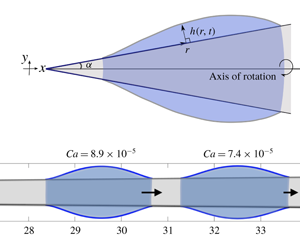
  $p_{co}-p_{o}=\unicode[STIX]{x1D6FE}\unicode[STIX]{x1D705}$. In this study, we provide a different physical picture to this phenomenon building on earlier seminal works on moving contact lines (Tanner Reference Tanner1979; Hocking Reference Hocking1983; Cox Reference Cox1986; Eggers Reference Eggers2004, Reference Eggers2005b); when a droplet is placed in contact with a conical fibre, it quickly adopts to a quasi-static shape of uniform pressure at the droplet scale. The conical geometry breaks the front/rear symmetry of the droplet shape. At the thicker part of the fibre, the apparent contact angle is larger than the equilibrium (microscopic) contact angle, thus a flow is generated and the contact line advances. The fluid recedes at the thinner part of the fibre, where the apparent contact angle is smaller than the equilibrium contact angle. Hence the droplet is expected to move from the tip to the base of a conical fibre, see figure 1. The pressure gradient in the bulk of the droplet only acts as a correction term for determining the droplet shape and plays a minor role on the dynamics.

Figure 1. Sketch of a droplet on a conical fibre with an angle  $\unicode[STIX]{x1D6FC}$. The droplet shape is described by the height $h(r,t)$ from the substrate to the free surface as a function of the radial distance from the vertex along the substrate $r$ and time $t$. At the contact line positions, i.e. $r=r_{r}$ and $r=r_{a}$, the free surface intersects with the substrate with an equilibrium (microscopic) contact angle $\unicode[STIX]{x1D703}_{e}$. The free surface deforms significantly in the vicinity of the contact line due to a large viscous stress. At the droplet scale, the contact angle appears as the apparent contact angles, $\unicode[STIX]{x1D703}_{r}$ at the thinner part of the cone (receding contact line) and $\unicode[STIX]{x1D703}_{a}$ at thicker part of the cone (advancing contact line).
We start our study by considering a viscous droplet of dynamic viscosity  $\unicode[STIX]{x1D702}$ that moves on a fibre when inertia can be neglected, i.e. Reynolds number, $Re\equiv ((\unicode[STIX]{x1D70C}UV^{1/3})/\unicode[STIX]{x1D702})\ll 1$ with the droplet size $V^{1/3}\ll (\unicode[STIX]{x1D6FE}/\unicode[STIX]{x1D70C}g)^{1/2}$. The motion is dominated by the capillary force but hindered by viscous friction, i.e. the capillary number $Ca\equiv (\unicode[STIX]{x1D702}U/\unicode[STIX]{x1D6FE})\ll 1$. A characteristic feature of slowly spreading viscous droplets is that it maintains a quasi-static shape during wetting (Tanner Reference Tanner1979; Bonn et al. Reference Bonn, Eggers, Indekeu, Meunier and Rolley2009), where viscous stresses are predominantly located in the vicinity of the contact line and balanced by the capillary stress through interface deformations. Together, this makes the problem well suited to be studied by the perturbation method of matched asymptotic expansions, which has been widely used to describe viscous spreading of droplets on flat substrates (Tanner Reference Tanner1979; Hocking & Rivers Reference Hocking and Rivers1982; Wilson Reference Wilson1982; Hocking Reference Hocking1983; Cox Reference Cox1986; Eggers Reference Eggers2004, Reference Eggers2005b; Pismen & Thiele Reference Pismen and Thiele2006; Savva & Kalliadasis Reference Savva and Kalliadasis2009; Snoeijer & Eggers Reference Snoeijer and Eggers2010; Chan, Gueudré & Snoeijer Reference Chan, Gueudré and Snoeijer2011). We develop here a similar approach, where we consider the viscous spreading of an axisymmetric droplet on a conical fibre by combining the lubrication theory and a perturbation method of asymptotic matching, to describe the directional droplet motion.
2 Mathematical formulation
We consider a droplet in contact with a solid conical fibre with an angle  $\unicode[STIX]{x1D6FC}$ as shown in figure 1. We assume the shape of the droplet is symmetric around the central axis of the cone. The droplet shape is described by the height $h(r,t)$ from the substrate to the free surface as a function of the radial distance from the vertex along the substrate $r$ and time $t$. As the droplet spontaneously starts to move on the cone, an incompressible viscous flow is generated. Since $Re\ll 1$, the flow inside the droplet is described by Stokes equations
 $$\begin{eqnarray}\displaystyle \unicode[STIX]{x1D702}\unicode[STIX]{x1D6FB}^{2}\boldsymbol{u}-\unicode[STIX]{x1D735}p=0, & & \displaystyle\end{eqnarray}$$
and the continuity equation reads
 $$\begin{eqnarray}\displaystyle \unicode[STIX]{x1D735}\boldsymbol{\cdot }\boldsymbol{u}=0, & & \displaystyle\end{eqnarray}$$
 where  $\boldsymbol{u}$ is the velocity and $p$ is the pressure. Moreover, we only consider small droplets, with a shape unaffected by gravity, i.e. the Bond number $Bo\equiv \unicode[STIX]{x1D70C}gV^{2/3}/\unicode[STIX]{x1D6FE}\ll 1$. We neglect any influence of the air surrounding the droplet as its viscosity is orders of magnitude smaller than the liquid viscosity.
To describe the fluid flow and the droplet motion, equations (2.1)–(2.2) need to be accompanied by several boundary conditions. At the free surface, the tangential stress is zero as we neglect the viscous effects in the air. The normal stress  $\unicode[STIX]{x1D70E}_{n}^{f}$ is described by the Young–Laplace law
 $$\begin{eqnarray}\unicode[STIX]{x1D70E}_{n}^{f}=\unicode[STIX]{x1D6FE}\unicode[STIX]{x1D705},\end{eqnarray}$$
 where  $\unicode[STIX]{x1D705}$ is the curvature of the interface.
At the wetted substrate, the normal velocity is zero and we assume a tangential velocity  $u_{t}^{s}$ described by the Navier slip condition (Lauga, Brenner & Stone Reference Lauga, Brenner, Stone, Tropea, Foss and Yarin2008)
 $$\begin{eqnarray}u_{t}^{s}=\frac{\unicode[STIX]{x1D706}}{\unicode[STIX]{x1D702}}\unicode[STIX]{x1D70E}_{t}^{s},\end{eqnarray}$$
 where  $\unicode[STIX]{x1D70E}_{t}^{s}$ is the shear stress parallel to the substrate and $\unicode[STIX]{x1D706}$ is the slip length. Slippage of fluid along the substrate is well known to regularize the viscous stress singularity at the moving contact line where the liquid, air and solid phase intersect. The slip length has been measured to be in a range of a few nanometres or less for simple fluids (Lauga et al. Reference Lauga, Brenner, Stone, Tropea, Foss and Yarin2008). Other models, such as the diffuse interface model (Qian, Wang & Sheng Reference Qian, Wang and Sheng2006; Carlson, Do-Quang & Amberg Reference Carlson, Do-Quang and Amberg2011), a precursor film (Eggers Reference Eggers2005a) and the molecular-kinetic theory (Blake Reference Blake2006) have been proposed to tackle the hydrodynamic singularity at the moving contact line. Nevertheless, like the slip length, these models introduce a characteristic length that is typically at the nanoscale, several orders of magnitude smaller than a droplet size of a few millimetres.
We also need to specify the slope of the free surface at the contact line. We assume that molecules at the contact lines quickly redistribute so that an equilibrium angle  $\unicode[STIX]{x1D703}_{e}$ is achieved and given by Young’s law $\cos \unicode[STIX]{x1D703}_{e}=(\unicode[STIX]{x1D6FE}_{SL}-\unicode[STIX]{x1D6FE}_{SV})/\unicode[STIX]{x1D6FE}$, and is independent of the contact line velocity, where $\unicode[STIX]{x1D6FE}_{SL}$ and $\unicode[STIX]{x1D6FE}_{SV}$ are, respectively, the liquid/solid and solid/air surface tension coefficients, as used in previous studies (Cox Reference Cox1986; Eggers Reference Eggers2005b; Duez et al. Reference Duez, Ybert, Clanet and Bocquet2007). The justification of this assumption is beyond the extent of our hydrodynamic model, and could be solved by other modelling approaches such as the diffuse interface model (Qian et al. Reference Qian, Wang and Sheng2006; Carlson et al. Reference Carlson, Do-Quang and Amberg2011) and molecular dynamics simulations (Johansson, Carlson & Hess Reference Johansson, Carlson and Hess2015). Moreover, the surface of the fibre is assumed to be chemically homogeneous and smooth, allowing us to neglect any contact angle hysteresis.
2.1 Lubrication approximation on a cone
For polar angles  $\unicode[STIX]{x1D703}\ll 1$ and an equilibrium contact angle $\unicode[STIX]{x1D703}_{e}\ll 1$, the flow inside the droplet is primarily in the radial direction and the droplet is fairly flat. By using these approximations, the Stokes equations (2.1) simplifies to the lubrication equations here given in spherical coordinates (a detailed derivation is given in A.1),
 $$\begin{eqnarray}\displaystyle & \displaystyle \frac{\unicode[STIX]{x2202}p}{\unicode[STIX]{x2202}r}=\frac{\unicode[STIX]{x1D702}}{r^{2}\unicode[STIX]{x1D703}}\frac{\unicode[STIX]{x2202}}{\unicode[STIX]{x2202}\unicode[STIX]{x1D703}}\left(\unicode[STIX]{x1D703}\frac{\unicode[STIX]{x2202}u}{\unicode[STIX]{x2202}\unicode[STIX]{x1D703}}\right), & \displaystyle\end{eqnarray}$$
 $$\begin{eqnarray}\displaystyle & \displaystyle \frac{\unicode[STIX]{x2202}p}{\unicode[STIX]{x2202}\unicode[STIX]{x1D703}}=0, & \displaystyle\end{eqnarray}$$
 where  $u=u(r,\unicode[STIX]{x1D703})$ is the radial velocity. The boundary conditions are
 $$\begin{eqnarray}\displaystyle & \displaystyle \frac{\unicode[STIX]{x2202}u}{\unicode[STIX]{x2202}\unicode[STIX]{x1D703}}=0\quad \text{at }\unicode[STIX]{x1D703}=\unicode[STIX]{x1D6FC}+\frac{h}{r}, & \displaystyle\end{eqnarray}$$
 $$\begin{eqnarray}\displaystyle & \displaystyle \frac{u}{\unicode[STIX]{x1D706}}=\frac{1}{r}\frac{\unicode[STIX]{x2202}u}{\unicode[STIX]{x2202}\unicode[STIX]{x1D703}}\quad \text{at }\unicode[STIX]{x1D703}=\unicode[STIX]{x1D6FC}. & \displaystyle\end{eqnarray}$$ $p$ is independent of $\unicode[STIX]{x1D703}$. Solving (2.5) and (2.6) with the boundary conditions (2.7) gives us the velocity
  $$\begin{eqnarray}\displaystyle u=\frac{r^{2}}{2\unicode[STIX]{x1D702}}\frac{\unicode[STIX]{x2202}p}{\unicode[STIX]{x2202}r}\left[\frac{\unicode[STIX]{x1D703}^{2}-\unicode[STIX]{x1D6FC}^{2}}{2}-\left(\unicode[STIX]{x1D6FC}+\frac{h}{r}\right)^{2}\ln \left(\frac{\unicode[STIX]{x1D703}}{\unicode[STIX]{x1D6FC}}\right)-\frac{\unicode[STIX]{x1D706}h}{\unicode[STIX]{x1D6FC}r^{2}}\left(2\unicode[STIX]{x1D6FC}+\frac{h}{r}\right)\right]. & & \displaystyle\end{eqnarray}$$
 The dynamics of the droplet’s interface, i.e.  $\unicode[STIX]{x1D703}=\unicode[STIX]{x1D6FC}+h(r,t)/r$, is obtained by imposing mass conservation of the liquid
 $$\begin{eqnarray}\displaystyle \frac{\unicode[STIX]{x2202}h}{\unicode[STIX]{x2202}t}+\frac{1}{r\unicode[STIX]{x1D6FC}+h}\frac{\unicode[STIX]{x2202}}{\unicode[STIX]{x2202}r}\int _{\unicode[STIX]{x1D6FC}}^{\unicode[STIX]{x1D6FC}+h/r}ur^{2}\unicode[STIX]{x1D703}\,\text{d}\unicode[STIX]{x1D703}=0. & & \displaystyle\end{eqnarray}$$
 The characteristic velocity scale  $U$ in the radial direction is much smaller than the capillary velocity $\unicode[STIX]{x1D6FE}/\unicode[STIX]{x1D702}$ as $Ca\ll 1$, see A.2 for a further description. Hence the free surface relaxes much faster than the motion of the droplet. We then expect that the spreading will be quasi-steady, and the entire droplet moves at a contact line velocity $u_{cl}$. In the frame of the moving droplet, the droplet shape is stationary for a small time increment, i.e. $\unicode[STIX]{x2202}h/\unicode[STIX]{x2202}t=0$, and the velocity inside the liquid is $u-u_{cl}$, hence we can reduce the time-dependent lubrication equation (2.9) to a stationary form
 $$\begin{eqnarray}\int _{\unicode[STIX]{x1D6FC}}^{\unicode[STIX]{x1D6FC}+h/r}(u-u_{cl})\unicode[STIX]{x1D703}\,\text{d}\unicode[STIX]{x1D703}=0.\end{eqnarray}$$
 In addition we have imposed a zero flux condition at the contact line. To evaluate (2.10), we substitute (2.3) and (2.8) with the normal stress  $\unicode[STIX]{x1D70E}_{n}^{f}=-p$ into (2.10) and get
 $$\begin{eqnarray}\frac{\unicode[STIX]{x2202}\unicode[STIX]{x1D705}}{\unicode[STIX]{x2202}r}=\frac{Ca}{F(h,r,\unicode[STIX]{x1D6FC},\unicode[STIX]{x1D706})},\end{eqnarray}$$
 with  $Ca=\unicode[STIX]{x1D702}u_{cl}/\unicode[STIX]{x1D6FE}$ and
 $$\begin{eqnarray}\displaystyle F(h,r,\unicode[STIX]{x1D6FC},\unicode[STIX]{x1D706})=\frac{r^{2}\unicode[STIX]{x1D6FC}^{2}}{2}\left[\frac{(1+\bar{\unicode[STIX]{x1D719}})^{4}}{\bar{\unicode[STIX]{x1D719}}(2+\bar{\unicode[STIX]{x1D719}})}\ln (1+\bar{\unicode[STIX]{x1D719}})-\frac{1}{4}(2+6\bar{\unicode[STIX]{x1D719}}+3\bar{\unicode[STIX]{x1D719}}^{2})+\bar{\unicode[STIX]{x1D706}}\bar{\unicode[STIX]{x1D719}}(2+\bar{\unicode[STIX]{x1D719}})\right],\quad & & \displaystyle\end{eqnarray}$$
 where  $\bar{\unicode[STIX]{x1D719}}=h/(\unicode[STIX]{x1D6FC}r)$ and $\bar{\unicode[STIX]{x1D706}}=\unicode[STIX]{x1D706}/(\unicode[STIX]{x1D6FC}r)$. In the limit of the film thickness being much smaller than the cone radius, i.e. $\bar{\unicode[STIX]{x1D719}}\ll 1$, $F\approx h(h+3\unicode[STIX]{x1D706})/3$. Hence (2.11) is reduced to the standard two-dimensional steady lubrication equation $\unicode[STIX]{x2202}\unicode[STIX]{x1D705}/\unicode[STIX]{x2202}r=3Ca/(h(h+3\unicode[STIX]{x1D706}))$. The curvature of the free surface $\unicode[STIX]{x1D705}$ is expressed as
 $$\begin{eqnarray}\unicode[STIX]{x1D705}=\frac{h^{\prime \prime }}{(1+h^{\prime 2})^{3/2}}-\frac{1-\unicode[STIX]{x1D6FC}h^{\prime }}{(r\unicode[STIX]{x1D6FC}+h)(1+h^{\prime 2})^{1/2}},\end{eqnarray}$$
 with  $()^{\prime }\equiv \unicode[STIX]{x2202}()/\unicode[STIX]{x2202}r$. We note the second term of the curvature is derived by using a rotation matrix with an angle $\unicode[STIX]{x1D6FC}\ll 1$, see the derivation in A.3. We use (2.13) as a description of the curvature as we will see in the following that the droplet shape away from the contact line is determined by $\unicode[STIX]{x1D705}=\text{constant}$.
The boundary conditions for  $h(r)$ at the receding contact line $r=r_{r}$ read
 $$\begin{eqnarray}\displaystyle & \displaystyle h(r=r_{r})=0, & \displaystyle\end{eqnarray}$$
 $$\begin{eqnarray}\displaystyle & \displaystyle h^{\prime }(r=r_{r})=\unicode[STIX]{x1D703}_{e}, & \displaystyle\end{eqnarray}$$ $r=r_{a}$ read
  $$\begin{eqnarray}\displaystyle & \displaystyle h(r=r_{a})=0, & \displaystyle\end{eqnarray}$$
 $$\begin{eqnarray}\displaystyle & \displaystyle h^{\prime }(r=r_{a})=-\unicode[STIX]{x1D703}_{e}. & \displaystyle\end{eqnarray}$$
 In the following, all the lengths are rescaled by  $V^{1/3}$ with the volume $V$ given by
 $$\begin{eqnarray}V=\unicode[STIX]{x03C0}\int _{r_{r}}^{r_{a}}h(h+2\unicode[STIX]{x1D6FC}r)\,\text{d}r.\end{eqnarray}$$
 For simplicity of notation, we keep the same symbols for all rescaled quantities, i.e.  $h$,
$h$,  $r$,
$r$,  $\unicode[STIX]{x1D706}$ and $\unicode[STIX]{x1D705}$. Note that (2.11)–(2.15) have the same forms after rescaling and the model parameters that dictate the dynamics are the cone angle $\unicode[STIX]{x1D6FC}$, the equilibrium contact angle $\unicode[STIX]{x1D703}_{e}$ and the slip length $\unicode[STIX]{x1D706}$. The droplet profile $h(r)$ and the capillary number $Ca$ are determined by solving (2.11) with the boundary conditions (2.14) and (2.15) by using the shooting method (Press et al. Reference Press, Teukolski, Vetterling and Flannery2007).
2.2 Asymptotic analysis
We now turn to a description based on the method of matched asymptotic expansions. The droplet size and the slip length differ by several orders of magnitude and we expect that the governing forces are different at these two length scales. In the vicinity of the contact line, denoted as the inner region, the flow is maintained by the balance of capillarity and the viscous force. Away from the contact line, the droplet is considered to be quasi-static with a shape only determined by the capillary force, denoted as the outer region. In the following, we summarize our analysis, which builds on the work by Eggers (Reference Eggers2005b) and this matching procedure has also been justified by a detailed analysis of the behaviour of the solutions in the framework of the lubrication approximation (Sibley, Nold & Kalliadasis Reference Sibley, Nold and Kalliadasis2015).
2.2.1 Inner solutions
In the inner regions, the characteristic length is the slip length  $\unicode[STIX]{x1D706}$, which is assumed to be much smaller than the local radius of curvature of the cone, i.e. $h\sim \unicode[STIX]{x1D706}\ll r\unicode[STIX]{x1D6FC}$, hence
 $$\begin{eqnarray}\displaystyle F(h,r,\unicode[STIX]{x1D6FC},\unicode[STIX]{x1D706})\approx \frac{1}{3}h(h+3\unicode[STIX]{x1D706})+O\left(\frac{h}{r\unicode[STIX]{x1D6FC}}\right). & & \displaystyle\end{eqnarray}$$
Equation (2.11) is then reduced to
 $$\begin{eqnarray}\frac{\unicode[STIX]{x2202}\unicode[STIX]{x1D705}}{\unicode[STIX]{x2202}r}=\frac{3Ca}{h(h+3\unicode[STIX]{x1D706})}.\end{eqnarray}$$
 We approximate the curvature of the free surface as  $\unicode[STIX]{x1D705}\approx h^{\prime \prime }\sim \unicode[STIX]{x1D703}_{e}^{2}/\unicode[STIX]{x1D706}>1/(r\unicode[STIX]{x1D6FC})$, equation (2.18) is then consistent with the lubrication equation for a two-dimensional flow (Batchelor Reference Batchelor1967; Oron, Davis & Bankoff Reference Oron, Davis and Bankoff1997). The behaviour of the solution of (2.18) has been discussed in detail by Eggers (Reference Eggers2005b). To match the solution in the outer region, only the asymptotic behaviour when $h$ is much larger than $\unicode[STIX]{x1D706}$ is required.
At the droplet’s trailing edge, i.e. the receding inner region, we define the interfacial profile as  $h_{r}=h_{r}(x_{r})$, where $x_{r}\equiv r-r_{r}$ is the distance along the substrate from the contact line position, i.e. the profile is determined by the lubrication equation
 $$\begin{eqnarray}h_{r}^{\prime \prime \prime }(x_{r})=\frac{3Ca}{h_{r}^{2}(x_{r})+3\unicode[STIX]{x1D706}h_{r}(x_{r})}.\end{eqnarray}$$
The prime symbol represents the derivative with respect to the independent variable. Equation (2.19) is complemented by the boundary conditions at the substrate where the height is
 $$\begin{eqnarray}h_{r}(x_{r}=0)=0,\end{eqnarray}$$
and the profile slope is given by the equilibrium angle
 $$\begin{eqnarray}h_{r}^{\prime }(x_{r}=0)=\unicode[STIX]{x1D703}_{e}.\end{eqnarray}$$
 By following the analysis by Eggers (Reference Eggers2005b), the asymptotic behaviour of  $h_{r}$ for $\unicode[STIX]{x1D703}_{e}x_{r}/\unicode[STIX]{x1D706}\gg 1$ is
 $$\begin{eqnarray}h_{r}(x_{r})=(3Ca)^{1/3}\left[\frac{\unicode[STIX]{x1D705}_{y}x_{r}^{2}}{6\unicode[STIX]{x1D706}}+b_{y}x_{r}\right],\end{eqnarray}$$
where
 $$\begin{eqnarray}\unicode[STIX]{x1D705}_{y}=\left(\frac{2^{1/6}\unicode[STIX]{x1D6FD}}{\unicode[STIX]{x03C0}Ai(s_{1})}\right)^{2},\quad b_{y}=\frac{-2^{2/3}Ai^{\prime }(s_{1})}{Ai(s_{1})},\quad \unicode[STIX]{x1D6FD}^{2}=\frac{\unicode[STIX]{x03C0}\exp [-\unicode[STIX]{x1D703}_{e}^{3}/(9Ca)]}{2^{2/3}}.\end{eqnarray}$$
 Here,  $Ai$ is the Airy function and $s_{1}$ needs to be determined from the asymptotic matching.
At the advancing droplet front,  $x_{a}\equiv r_{a}-r$ is defined as the distance from the contact line along the substrate, and has a profile $h_{a}=h_{a}(x_{a})$ described by
 $$\begin{eqnarray}h_{a}^{\prime \prime \prime }(x_{a})=-\frac{3Ca}{h_{a}^{2}(x_{a})+3\unicode[STIX]{x1D706}h_{a}(x_{a})},\end{eqnarray}$$
and complemented with the boundary conditions at the substrate where the height is
 $$\begin{eqnarray}h_{a}(x_{a}=0)=0,\end{eqnarray}$$
and the slope is given by the equilibrium angle
 $$\begin{eqnarray}h_{a}^{\prime }(x_{a}=0)=\unicode[STIX]{x1D703}_{e}.\end{eqnarray}$$
 The asymptotic behaviour for  $\unicode[STIX]{x1D703}_{e}x_{a}/\unicode[STIX]{x1D706}\gg 1$ is in a functional form of the Cox–Voinov relation (Eggers Reference Eggers2005b)
 $$\begin{eqnarray}h_{a}^{\prime }(x_{a})^{3}=\unicode[STIX]{x1D703}_{e}^{3}+9Ca\ln (e\unicode[STIX]{x1D703}_{e}x_{a}/3\unicode[STIX]{x1D706}),\end{eqnarray}$$
 where  $e=2.7182\ldots$ is Euler’s number.
2.2.2 Outer solution
At the length scale of the droplet size, i.e. the outer region, the dominant force is capillarity. Viscous effects appear only as a small correction in the higher-order terms of  $Ca$ as we have $Ca\ll 1$. We define the outer solution as $\bar{h}(r)$ and expand it in series of $Ca$
$Ca$
 $$\begin{eqnarray}\bar{h}(r)=\bar{h}_{0}(r)+Ca\bar{h}_{1}(r)+O(Ca^{2}).\end{eqnarray}$$
 We solve for the leading-order term  $\bar{h}_{0}(r)$ from the condition of uniform interfacial curvature $\unicode[STIX]{x1D705}_{0}$, which can be expressed by the relation
 $$\begin{eqnarray}\unicode[STIX]{x1D705}_{0}=\frac{\bar{h}_{0}^{\prime \prime }}{(1+\bar{h}_{0}^{\prime 2})^{3/2}}-\frac{1-\unicode[STIX]{x1D6FC}\bar{h}_{0}^{\prime }}{(r\unicode[STIX]{x1D6FC}+\bar{h}_{0})(1+\bar{h}_{0}^{\prime 2})^{1/2}}.\end{eqnarray}$$
 Note that this expression is the same as (2.13) with a replacement of  $h(r)$ by $\bar{h}_{0}(r)$. The value of the curvature $\unicode[STIX]{x1D705}_{0}$ depends on the position of the droplet and is determined together with the relation between the volume $V_{0}$ and the profile $\bar{h}_{0}$ of the droplet, that is
 $$\begin{eqnarray}V_{0}=\unicode[STIX]{x03C0}\int _{r_{r}}^{r_{a}}\bar{h}_{0}(\bar{h}_{0}+2\unicode[STIX]{x1D6FC}r)\,\text{d}r.\end{eqnarray}$$
 The contact angle of the static profile  $\bar{h}_{0}(r)$ with the substrate at the receding part is used to define the receding apparent contact angle $\unicode[STIX]{x1D703}_{r}$, while the advancing droplet edge is defined by the advancing apparent contact angle $\unicode[STIX]{x1D703}_{a}$. Two boundary conditions are required to solve the second-order ordinary differential equation (2.29), where we impose the following conditions at the receding contact line:
 $$\begin{eqnarray}\displaystyle & \displaystyle \bar{h}_{0}(r=r_{r})=0, & \displaystyle\end{eqnarray}$$
 $$\begin{eqnarray}\displaystyle & \displaystyle \bar{h}_{0}^{\prime }(r=r_{r})=\unicode[STIX]{x1D703}_{r}. & \displaystyle\end{eqnarray}$$
The position of the advancing contact line and the advancing apparent contact angle are given by the conditions
 $$\begin{eqnarray}\displaystyle & \displaystyle \bar{h}_{0}(r=r_{a})=0, & \displaystyle\end{eqnarray}$$
 $$\begin{eqnarray}\displaystyle & \displaystyle \bar{h}_{0}^{\prime }(r=r_{a})=-\unicode[STIX]{x1D703}_{a}. & \displaystyle\end{eqnarray}$$
 To match to the inner solution at the receding contact line region, only the leading-order term  $\bar{h}_{0}(r)$, i.e. the static profile, is required. The asymptotic behaviour of $\bar{h}_{0}(r)$ near the contact line is determined by a Taylor expansion:
 $$\begin{eqnarray}\bar{h}_{0}(r)=\unicode[STIX]{x1D703}_{r}(r-r_{r})+{\textstyle \frac{1}{2}}\unicode[STIX]{x1D705}_{r}(r-r_{r})^{2}+O((r-r_{r})^{3}).\end{eqnarray}$$
 At the advancing droplet front, the first-order correction  $\bar{h}_{1}(r)$ is required in order to match to the logarithmic behaviour of the inner solution in (2.27) (Eggers Reference Eggers2005b). However, there is no analytical solution for the correction term for a cone geometry. Instead of computing the exact expression as done by Eggers (Reference Eggers2005b) for a flat substrate, we assume that the outer solution near the advancing contact line has the functional form
 $$\begin{eqnarray}\bar{h}^{\prime 3}=\unicode[STIX]{x1D703}_{a}^{3}+9Ca\ln [c_{a}(r_{a}-r)],\end{eqnarray}$$
 where  $c_{a}$ is an adjustable parameter but appears in the logarithm and has only a weak effect on the results. The excellent agreement between the results from matching and the numerical results from solving the full lubrication equation suggests that the assumption we have made here is justified.
2.2.3 Matching the inner and the outer solutions
We are now in a position to perform the matching between the asymptotic behaviour of the inner and outer solutions to determine the unknown quantities,  $Ca$,
$Ca$,  $s_{1}$ and $\unicode[STIX]{x1D703}_{r}$. To do this, we see that three matching conditions are required. By comparing the asymptotic behaviour of the inner solution (2.22) and the outer solution (2.35) at the receding region, we find the matching conditions
 $$\begin{eqnarray}\displaystyle & \displaystyle \unicode[STIX]{x1D703}_{r}=(3Ca)^{1/3}b_{y}, & \displaystyle\end{eqnarray}$$
 $$\begin{eqnarray}\displaystyle & \displaystyle \unicode[STIX]{x1D705}_{r}=\frac{(3Ca)^{1/3}\unicode[STIX]{x1D705}_{y}}{3\unicode[STIX]{x1D706}}. & \displaystyle\end{eqnarray}$$
At the advancing contact line region, we match the inner solution (2.27) to the outer solution (2.36). This procedure of matching the cubes of the free surface slope has been shown to be justified for these flows described by lubrication theory (Sibley et al. Reference Sibley, Nold and Kalliadasis2015). The advancing apparent contact angle becomes
 $$\begin{eqnarray}\unicode[STIX]{x1D703}_{a}^{3}=\unicode[STIX]{x1D703}_{e}^{3}+9Ca\ln (c/\unicode[STIX]{x1D706}),\end{eqnarray}$$
 with  $c\equiv e\unicode[STIX]{x1D703}_{e}/3c_{a}$ that is treated as an adjustable parameter. We fix $c=0.04$ when $\unicode[STIX]{x1D703}_{e}=0.2~\text{rad}$ by fitting the results of asymptotic matching and lubrication approximation. We also find that $c$ depends on $\unicode[STIX]{x1D703}_{e}$, and we use $c=0.027$ when $\unicode[STIX]{x1D703}_{e}=0.3~\text{rad}$ and $c=0.007$ when $\unicode[STIX]{x1D703}_{e}=0.4~\text{rad}$ (see § 3).

Figure 2. (a) The blue curves are the droplet shapes predicted by the lubrication approximation on a cone for a slip length  $\unicode[STIX]{x1D706}=10^{-6}$ and $\unicode[STIX]{x1D6FC}=0.01$. The grey area represents the conical fibre. Here, $x$ and $y$ are the coordinates, respectively, along and perpendicular to the axis of rotation. The equilibrium contact angle is $\unicode[STIX]{x1D703}_{e}=0.2~\text{rad}$ (11. 5°). The cone angle is $\unicode[STIX]{x1D6FC}=0.01~\text{rad}$ (0. 57°), similar to the experiments by Lorenceau & Quéré (Reference Lorenceau and Quéré2004). (b) The droplet capillary number as a function of the droplet’s centre of mass $x_{cm}$ for three different slip lengths using the LAC and the asymptotic matching. (c) The receding apparent contact angle $\unicode[STIX]{x1D703}_{r}$ as a function of $Ca$ computed by asymptotic matching. The vertical dotted lines indicate the critical capillary numbers $Ca_{c}$.
2.2.4 Completely wetting substrate,  $\unicode[STIX]{x1D703}_{e}=0~\text{rad}$

In the case of a completely wetting droplet, a Landau–Levich–Derjaguin film (Landau & Levich Reference Landau and Levich1942; de Gennes Reference de Gennes1985) will be deposited on the substrate at the receding contact line as the droplet moves. We can assume that the receding apparent contact angle  $\unicode[STIX]{x1D703}_{r}$ is zero for any value of $Ca$ and matching at the receding region is not needed. The advancing apparent contact angle $\unicode[STIX]{x1D703}_{a}$ is obtained by solving for the static outer solution governed by (2.29) with $\unicode[STIX]{x1D703}_{r}=0~\text{rad}$. Once $\unicode[STIX]{x1D703}_{a}$ is computed, the capillary number $Ca$ is determined by the condition (2.39) at the advancing contact line
 $$\begin{eqnarray}Ca=\frac{\unicode[STIX]{x1D703}_{a}^{3}}{9\ln (c/\unicode[STIX]{x1D706})}.\end{eqnarray}$$
3 Results
Next, we solve the two mathematical models, the lubrication approximation on a cone (LAC) and the asymptotic matching (AM), to predict the directional spreading dynamics of droplets on a conical fibre. There are several physical parameters that can influence the spreading phenomenon, the cone angle  $\unicode[STIX]{x1D6FC}$, the slip length $\unicode[STIX]{x1D706}$ and the equilibrium contact angle $\unicode[STIX]{x1D703}_{e}$ and we show how these parameters influence the dynamics, i.e. the droplet’s capillary number $Ca$ and shape. The LAC given by (2.11)–(2.13) is solved by using the shooting method with boundary conditions (2.14), (2.15) and the constant volume condition (2.16). The solution for the AM is obtained by solving the matching conditions (2.37)–(2.39) together with the uniform curvature condition (2.29) and the constant volume condition (2.30) for the static outer solution, which allows us to determine $Ca$,
$Ca$,  $s_{1}$, $\unicode[STIX]{x1D703}_{r}$ and $\unicode[STIX]{x1D703}_{a}$. The droplet centre of mass $x_{cm}$ is used to quantify its position on the cone and is given by
 $$\begin{eqnarray}x_{cm}=\unicode[STIX]{x03C0}\int _{r_{r}}^{r_{a}}h(h+2\unicode[STIX]{x1D6FC}r)r\,\text{d}r.\end{eqnarray}$$
3.1 Droplet spreading velocity on a cone
The droplet shape during directional spreading is shown in figure 2(a), where the droplet moves from left to right for a cone with radius  $R=\unicode[STIX]{x1D6FC}x$, i.e. the droplet moves to the thicker part of the cone but decelerates along the way, qualitatively consistent with experimental measurements (Lorenceau & Quéré Reference Lorenceau and Quéré2004). We start by determining the droplet velocity along the cone, illustrated by the capillary number $Ca$ as a function of $x_{cm}$ and shown for different slip lengths in figure 2(b). The predictions from the two mathematical models (LAC and AM) are in excellent agreement although the slip length is varied by two orders of magnitude. We see that the droplet velocity is not a linear function of the cone radius $R$ and there exists a critical capillary number $Ca_{c}$ above which no solution is predicted by the LAC or the AM. To understand why no solution is found, we show the receding apparent contact angle $\unicode[STIX]{x1D703}_{r}$ as predicted by asymptotic matching as a function of $Ca$ in figure 2(c). The receding contact angle approaches zero as the capillary number gets closer to the critical value $Ca\rightarrow Ca_{c}$. A vanishing receding contact angle implies that a film is formed at the droplet tail (Cox Reference Cox1986; Eggers Reference Eggers2004; Snoeijer et al. Reference Snoeijer, Ziegler, Andreotti, Fermigier and Eggers2008). Also the slip length $\unicode[STIX]{x1D706}$ can influence the spreading, but its influence on the results is weaker than the other parameters in the system and primarily influence the results for larger $Ca$, in concordance with other moving contact line models (Cox Reference Cox1986; Eggers Reference Eggers2005b; Snoeijer & Andreotti Reference Snoeijer and Andreotti2013) as $\unicode[STIX]{x1D706}$ appears in the logarithmic term in (2.39).

Figure 3. The capillary number  $Ca$ plotted as a function of the droplet’s centre of mass $x_{cm}$ for four different equilibrium contact angles $\unicode[STIX]{x1D703}_{e}$, predicted by the lubrication approximation on a cone and by the asymptotic matching. The three symbols in black indicate the critical capillary numbers above which the film deposition occurs. The slip length $\unicode[STIX]{x1D706}=10^{-6}$ and the cone angle $\unicode[STIX]{x1D6FC}=0.01~\text{rad}$ (0. 57°). Note that the completely wetting $\unicode[STIX]{x1D703}_{e}=0~\text{rad}$ is a special case as a Landau–Levich–Derjaguin (known as LLD) film is deposited on the substrate surface. The values of $c$ used in AM for $\unicode[STIX]{x1D703}_{e}=0$, 0.2, 0.3 and 0.4 rad, respectively, are 0.07, 0.04, 0.027 and 0.007.
The droplet wettability, i.e. the equilibrium contact angle  $\unicode[STIX]{x1D703}_{e}$ also influences the spreading dynamics and we solve the droplet velocity for different $\unicode[STIX]{x1D703}_{e}$, see figure 3. For partially wetting droplets, the capillary number $Ca$ increases with $\unicode[STIX]{x1D703}_{e}$ when compared at the same droplet position. The completely wetting droplet $\unicode[STIX]{x1D703}_{e}=0~\text{rad}$ is a special case in figure 3, with $\unicode[STIX]{x1D703}_{r}=0~\text{rad}$ at any position $x_{cm}$ on the cone, as a Landau–Levich–Derjaguin film formed at the receding contact line (de Gennes Reference de Gennes1985). We can then compare a completely wetting droplet with a partially wetting droplet at $\unicode[STIX]{x1D703}_{r}=0~\text{rad}$ and at the same position on the conical fibre. Here, the macroscopic droplet shapes would be the same, as well as their advancing apparent contact angle, but the droplet velocity is determined by (2.39) explaining why a completely wetting droplet moves faster than a partially wetting droplet.
To illustrate the dependence on the slope of the cone by varying  $\unicode[STIX]{x1D6FC}$, we first define $R_{cm}$ as the cone radius at the droplet’s centre of mass,
 $$\begin{eqnarray}R_{cm}=x_{cm}\unicode[STIX]{x1D6FC}.\end{eqnarray}$$
 Equation (3.2) allows us to compare  $Ca$ for different $\unicode[STIX]{x1D6FC}$ at the same cone thickness $R_{cm}$, as shown in figure 4. As expected, the droplet moves faster when $\unicode[STIX]{x1D6FC}$ is larger for the same $R_{cm}$. Our results highlight how the droplet velocity can be tuned by the control of the macroscopic geometry of the conical substrate shape.

Figure 4. The capillary number  $Ca$ as a function of the cone radius $R_{cm}$ evaluated at the droplet’s centre of mass for three different cone angles $\unicode[STIX]{x1D6FC}$ by using the approaches of lubrication approximation on a cone and the asymptotic matching. The slip length $\unicode[STIX]{x1D706}=10^{-6}$ and the equilibrium contact angle $\unicode[STIX]{x1D703}_{e}=0.2~\text{rad}$.
3.2 Mismatch between the apparent and equilibrium contact angle
Since the motion of the droplet is generated by the capillary force, which depends on the interfacial curvature, we would like to know how the droplet shape maintains the viscous flow. In figure 5(a), the interface shape is plotted at a scale similar to the droplet size. We see that the prediction from the two theoretical approaches (LAC and AM) are in excellent agreement, illustrating that the droplet shape is quasi-static. In the contact line regions, it is expected that the viscous stress is balanced by the capillary stress. We show the droplet shape and the slopes of the droplet profile in the receding and the advancing contact line regions as a function of the distance from the contact line positions, see figures 5(b) and 5(c). In the advancing contact line region, we compare the results from the LCA and the AM in the form of the Cox–Voinov relation (Voinov Reference Voinov1976; Cox Reference Cox1986; Eggers Reference Eggers2005b). The good agreement between LAC and AM suggests that the force balance assumption in the contact line regions is correct. The interface deforms significantly near the contact lines. Large Laplace pressure gradients are generated to maintain the flow inside the two contact line regions. This large interfacial deformation is clearly illustrated in figure 6, where the local slope of the interface is plotted as a function of the distance from the contact line. As we can see from the curve computed by the LAC in figure 6(a), the local interface slope decreases from the equilibrium value ( $\unicode[STIX]{x1D703}_{e}=0.2~\text{rad}$) at the receding contact line position to a local minimum within a very small distance. The variation of local angle is due to the difference between the equilibrium contact angle and the receding apparent contact angle ( $\unicode[STIX]{x1D703}_{r}=0.12~\text{rad}$) determined from the macroscopic shape, see figure 6(a). In the advancing region, since the apparent contact angle is larger than the equilibrium angle, the interface slope increases with the distance from the contact line position, see figure 6(b). The flow and the droplet motion is generated by the mismatch of the equilibrium and apparent contact angles at the receding and the advancing contact lines. Because of the asymmetry of the conical shape, the apparent contact angle at the thicker part of the cone is larger than that at the thinner part and the droplet moves spontaneously from the thinner part to the thicker part.

Figure 5. (a) The droplet shape predicted by the lubrication approximation on a cone  $h(r)$ and the asymptotic matching $\bar{h}_{0}(r)$ for a slip length $\unicode[STIX]{x1D706}=10^{-6}$, the equilibrium contact angle $\unicode[STIX]{x1D703}_{e}=0.2~\text{rad}$ and the cone angle $\unicode[STIX]{x1D6FC}=0.01~\text{rad}$. The centre of mass of the droplet is $x_{cm}=30.0$ and the capillary number Ca = 8. 1 × 10⁻⁵. Here, $r_{r}$ and $r_{a}$ are, respectively, the receding and advancing contact line positions. (b) The droplet shape $h(r)$ plotted as a function of distance from the receding contact line in log–log scale. The curve for AM is the inner solution $h_{r}(x_{r})$ from (2.22). (c) Comparison between LAC and AM in the advancing contact line region. The curve for AM is from (2.27), ${\hat{h}}^{\prime }=-h^{\prime }(r)$ for the LAC and ${\hat{h}}^{\prime }=h_{a}^{\prime }(x_{a})$ for the AM. Note that (2.22) and (2.27) are the asymptotic behaviour of the inner solutions when $\unicode[STIX]{x1D703}_{e}x_{r}\gg \unicode[STIX]{x1D706}$ or $\unicode[STIX]{x1D703}_{e}x_{a}\gg \unicode[STIX]{x1D706}$. The solution of LAC is not captured by (2.22) when $x_{r}\rightarrow 0$ and (2.27) when $x_{a}\rightarrow 0$.

Figure 6. (a) The interface slope ( $h^{\prime }$ for LAC and $\bar{h}_{0}^{\prime }$ for AM) plotted as a function of the distance from the receding contact line position $r-r_{r}$ in logarithmic scale. The slip length $\unicode[STIX]{x1D706}=10^{-6}$, the equilibrium contact angle $\unicode[STIX]{x1D703}_{e}=0.2~\text{rad}$ and the cone angle $\unicode[STIX]{x1D6FC}=0.01~\text{rad}$. The centre of mass of the droplet is $x_{cm}=30.0$ and the capillary number Ca = 8. 1 × 10⁻⁵. Black line, solution obtained by lubrication approximation on a cone; Red dashed line, the outer solution obtained by asymptotic matching. (b) The predicted slopes from the LAC and the AM are plotted as a function of the distance from the advancing contact line.
4 Discussion and conclusions
We have shown that the motion of a fairly flat and viscous droplet on a conical fibre is driven by the difference between the equilibrium and the apparent contact angle, which is not the same at the advancing front and the receding tail. Moreover, our analysis shows that the capillary pressure gradient at the scale of the droplet size is very small and scales with  $Ca\ll 1$, which predicts a quasi-static droplet shape. Instead, large pressure gradients and strong interfacial deformations are found in the vicinity of the contact line, along with the dominant part of the viscous stresses. Our findings contrast the model proposed by Lorenceau & Quéré (Reference Lorenceau and Quéré2004) that is based on a capillary pressure gradient at the drop scale to generate the droplet motion, which for complete wetting is described by the relation
 $$\begin{eqnarray}Ca\sim \frac{h_{m}}{(r_{a}-r_{r})R_{cm}^{3}},\end{eqnarray}$$
 where  $h_{m}\equiv \max (h)$ is the maximum height of the droplet. We plot our results for the completely wetting case $\unicode[STIX]{x1D703}_{e}=0~\text{rad}$ and compare the results with the prediction (4.1) for several different cone angles $\unicode[STIX]{x1D6FC}$ in figure 7. The first observation we make, is that our predictions do not follow the relation (4.1). However, our results point to the possibility that if measurements are made over a limited range of $Ca$ or $h_{m}/((r_{a}-r_{r})R_{cm}^{3})$ the interpretation of the data can easily be misinterpreted to follow (4.1) in particular for larger cone angles.
A mismatch between the equilibrium contact angle and the apparent contact angle is found to dominate the flow and since this difference is not the same at the receding tail and advancing front a directional droplet spreading motion is generated. Although the equilibrium contact angle is constant on the conical fibre, the apparent angle changes due to its macroscopic asymmetric shape. Our model provides a general description of droplet motion on a conical substrate and can help to better understand droplet motion on slender geometries with varying shapes, which are found in an abundance of engineering systems as well as in nature.

Figure 7. The capillary number  $Ca$ is computed by using asymptotic matching with (2.40) for a completely wetting droplet as a function of the quantity $h_{m}/(r_{a}-r_{r})R_{cm}^{3}$. The slip length is $\unicode[STIX]{x1D706}=10^{-6}$. The straight line has a linear slope.
Acknowledgements
T.S.C. and A.C. gratefully acknowledge financial support from the UiO: Life Science initiative at the University of Oslo. F.Y. is grateful for support from the National Science Foundation (DMS-1514606). A.C. is grateful for the financial support from the Norwegian Research Council (263056, 301138). We thank C. Fournier and K. Dalnoki-Veress for stimulating discussions.
Declaration of interests
The authors report no conflict of interest.
Appendix A.
A.1 Derivation of the lubrication equations on a cone
We here give the details of the derivation of the lubrication equations. For axisymmetric flow, the fluid velocity is described by  $\boldsymbol{u}=u(\tilde{r},\unicode[STIX]{x1D703})\boldsymbol{e}_{\tilde{r}}+w(\tilde{r},\unicode[STIX]{x1D703})\boldsymbol{e}_{\unicode[STIX]{x1D703}}$, where $\tilde{r}$ and $\unicode[STIX]{x1D703}$ are, respectively, the radial distance and the polar angle in spherical coordinates, and the corresponding unit vectors are $\boldsymbol{e}_{\tilde{r}}$ and $\boldsymbol{e}_{\unicode[STIX]{x1D703}}$. The vertex of the cone is defined as the origin of the coordinate system, giving the Stokes equation as
 $$\begin{eqnarray}\displaystyle \frac{1}{\unicode[STIX]{x1D702}}\frac{\unicode[STIX]{x2202}p}{\unicode[STIX]{x2202}\tilde{r}}=\frac{1}{\tilde{r}^{2}}\left[\frac{\unicode[STIX]{x2202}}{\unicode[STIX]{x2202}\tilde{r}}\left(\tilde{r}^{2}\frac{\unicode[STIX]{x2202}u}{\unicode[STIX]{x2202}\tilde{r}}\right)+\frac{1}{\sin \unicode[STIX]{x1D703}}\frac{\unicode[STIX]{x2202}}{\unicode[STIX]{x2202}\unicode[STIX]{x1D703}}\left(\sin \unicode[STIX]{x1D703}\frac{\unicode[STIX]{x2202}u}{\unicode[STIX]{x2202}\unicode[STIX]{x1D703}}\right)\right]-\frac{2}{\tilde{r}^{2}}\left(u+\frac{\unicode[STIX]{x2202}w}{\unicode[STIX]{x2202}\unicode[STIX]{x1D703}}+w\cot \unicode[STIX]{x1D703}\right) & & \displaystyle\end{eqnarray}$$
and
 $$\begin{eqnarray}\displaystyle \frac{1}{\unicode[STIX]{x1D702}}\frac{\unicode[STIX]{x2202}p}{\unicode[STIX]{x2202}\unicode[STIX]{x1D703}}=\frac{1}{\tilde{r}}\left[\frac{\unicode[STIX]{x2202}}{\unicode[STIX]{x2202}\tilde{r}}\left(\tilde{r}^{2}\frac{\unicode[STIX]{x2202}w}{\unicode[STIX]{x2202}\tilde{r}}\right)+\frac{1}{\sin \unicode[STIX]{x1D703}}\frac{\unicode[STIX]{x2202}}{\unicode[STIX]{x2202}\unicode[STIX]{x1D703}}\left(\sin \unicode[STIX]{x1D703}\frac{\unicode[STIX]{x2202}w}{\unicode[STIX]{x2202}\unicode[STIX]{x1D703}}\right)\right]-\frac{2}{\tilde{r}}\left(\frac{w}{2\sin ^{2}\unicode[STIX]{x1D703}}-\frac{\unicode[STIX]{x2202}u}{\unicode[STIX]{x2202}\unicode[STIX]{x1D703}}\right). & & \displaystyle\end{eqnarray}$$
The continuity equation reads
 $$\begin{eqnarray}\displaystyle \frac{1}{\tilde{r}^{2}}\frac{\unicode[STIX]{x2202}}{\unicode[STIX]{x2202}\tilde{r}}(\tilde{r}^{2}u)+\frac{1}{\tilde{r}\sin \unicode[STIX]{x1D703}}\frac{\unicode[STIX]{x2202}}{\unicode[STIX]{x2202}\unicode[STIX]{x1D703}}(w\sin \unicode[STIX]{x1D703})=0. & & \displaystyle\end{eqnarray}$$
 Next we perform a lubrication approximation by considering small polar angles  $\unicode[STIX]{x1D703}\ll 1$ and a small equilibrium contact angle $\unicode[STIX]{x1D703}_{e}\ll 1$. In order to estimate the magnitude of each term in (A 1) and (A 2), we introduce the following rescaled quantities:
 $$\begin{eqnarray}\displaystyle \unicode[STIX]{x1D703}^{\ast }=\frac{\unicode[STIX]{x1D703}}{\unicode[STIX]{x1D716}},\quad h^{\ast }=\frac{h}{H},\quad \tilde{r}^{\ast }=\frac{\unicode[STIX]{x1D716}\tilde{r}}{H},\quad u^{\ast }=\frac{u}{U},\quad w^{\ast }=\frac{w}{W},\quad p^{\ast }=\frac{p}{P}. & & \displaystyle \nonumber\end{eqnarray}$$
 Here  $\unicode[STIX]{x1D716}\ll 1$, is the characteristic magnitude of the interfacial slope, for example, one possible choice is to define it as the spatial average of the interfacial slope. Here, $H$ is the characteristic scale of the droplet thickness. The radial distance $\tilde{r}$ is then rescaled by $H/\unicode[STIX]{x1D716}$. The scales for the radial velocity, the polar velocity and the pressure are represented by $U$,
$U$,  $W$ and $P$, respectively. Rewriting the continuity equation as
 $$\begin{eqnarray}\displaystyle \frac{\unicode[STIX]{x1D716}U}{\tilde{r}^{\ast 2}}\frac{\unicode[STIX]{x2202}}{\unicode[STIX]{x2202}\tilde{r}^{\ast }}(\tilde{r}^{\ast 2}u^{\ast })+\frac{W}{\tilde{r}^{\ast }\sin (\unicode[STIX]{x1D716}\unicode[STIX]{x1D703}^{\ast })}\frac{\unicode[STIX]{x2202}}{\unicode[STIX]{x2202}\unicode[STIX]{x1D703}^{\ast }}[w^{\ast }\sin (\unicode[STIX]{x1D716}\unicode[STIX]{x1D703}^{\ast })]=0, & & \displaystyle\end{eqnarray}$$
 we see the polar velocity scales as  $W\sim \unicode[STIX]{x1D716}U$. Using the rescaled quantities, the Stokes equations become
 $$\begin{eqnarray}\displaystyle \frac{PH}{\unicode[STIX]{x1D702}U\unicode[STIX]{x1D716}}\frac{\unicode[STIX]{x2202}p^{\ast }}{\unicode[STIX]{x2202}\tilde{r}^{\ast }} & = & \displaystyle \frac{1}{\tilde{r}^{\ast 2}}\left[\frac{\unicode[STIX]{x2202}}{\unicode[STIX]{x2202}\tilde{r}^{\ast }}\left(\tilde{r}^{\ast 2}\frac{\unicode[STIX]{x2202}u^{\ast }}{\unicode[STIX]{x2202}\tilde{r}^{\ast }}\right)+\frac{1}{\unicode[STIX]{x1D716}^{2}\sin (\unicode[STIX]{x1D716}\unicode[STIX]{x1D703}^{\ast })}\frac{\unicode[STIX]{x2202}}{\unicode[STIX]{x2202}\unicode[STIX]{x1D703}^{\ast }}\left(\sin (\unicode[STIX]{x1D716}\unicode[STIX]{x1D703}^{\ast })\frac{\unicode[STIX]{x2202}u^{\ast }}{\unicode[STIX]{x2202}\unicode[STIX]{x1D703}^{\ast }}\right)\right]\nonumber\\ \displaystyle & & \displaystyle -\,\frac{2}{\tilde{r}^{\ast 2}}\left(u^{\ast }+\frac{\unicode[STIX]{x2202}w^{\ast }}{\unicode[STIX]{x2202}\unicode[STIX]{x1D703}^{\ast }}+\unicode[STIX]{x1D716}w^{\ast }\cot (\unicode[STIX]{x1D716}\unicode[STIX]{x1D703}^{\ast })\right)\end{eqnarray}$$
 $$\begin{eqnarray}\displaystyle \frac{PH}{\unicode[STIX]{x1D702}U\unicode[STIX]{x1D716}^{2}}\frac{\unicode[STIX]{x2202}p^{\ast }}{\unicode[STIX]{x2202}\unicode[STIX]{x1D703}^{\ast }} & = & \displaystyle \frac{1}{\tilde{r}^{\ast }}\left[\frac{\unicode[STIX]{x1D716}\unicode[STIX]{x2202}}{\unicode[STIX]{x2202}\tilde{r}^{\ast }}\left(\tilde{r}^{\ast 2}\frac{\unicode[STIX]{x2202}w^{\ast }}{\unicode[STIX]{x2202}\tilde{r}^{\ast }}\right)+\frac{1}{\unicode[STIX]{x1D716}\sin (\unicode[STIX]{x1D716}\unicode[STIX]{x1D703}^{\ast })}\frac{\unicode[STIX]{x2202}}{\unicode[STIX]{x2202}\unicode[STIX]{x1D703}^{\ast }}\left(\sin (\unicode[STIX]{x1D716}\unicode[STIX]{x1D703}^{\ast })\frac{\unicode[STIX]{x2202}w^{\ast }}{\unicode[STIX]{x2202}\unicode[STIX]{x1D703}^{\ast }}\right)\right]\nonumber\\ \displaystyle & & \displaystyle -\,\frac{2}{\tilde{r}^{\ast }}\left(\frac{\unicode[STIX]{x1D716}w^{\ast }}{2\sin ^{2}(\unicode[STIX]{x1D716}\unicode[STIX]{x1D703}^{\ast })}+\frac{\unicode[STIX]{x2202}u^{\ast }}{\unicode[STIX]{x1D716}\unicode[STIX]{x2202}\unicode[STIX]{x1D703}^{\ast }}\right).\end{eqnarray}$$
 We expect that the pressure gradient  $\unicode[STIX]{x2202}p^{\ast }/\unicode[STIX]{x2202}\tilde{r}^{\ast }$ drives the flow. To balance the leading-order terms on the right-hand side of (A 5), $P=\unicode[STIX]{x1D702}U/(\unicode[STIX]{x1D716}H)$. Since $\unicode[STIX]{x1D716}\ll 1$, keeping only the leading-order terms, equation (A 5) becomes
 $$\begin{eqnarray}\displaystyle \frac{\unicode[STIX]{x2202}p^{\ast }}{\unicode[STIX]{x2202}\tilde{r}^{\ast }}=\frac{1}{\tilde{r}^{\ast 2}}\frac{1}{\unicode[STIX]{x1D703}^{\ast }}\frac{\unicode[STIX]{x2202}}{\unicode[STIX]{x2202}\unicode[STIX]{x1D703}^{\ast }}\left(\unicode[STIX]{x1D703}^{\ast }\frac{\unicode[STIX]{x2202}u^{\ast }}{\unicode[STIX]{x2202}\unicode[STIX]{x1D703}^{\ast }}\right), & & \displaystyle\end{eqnarray}$$
and (A 6) becomes
 $$\begin{eqnarray}\displaystyle \frac{\unicode[STIX]{x2202}p^{\ast }}{\unicode[STIX]{x2202}\unicode[STIX]{x1D703}^{\ast }}=0. & & \displaystyle\end{eqnarray}$$
 In spherical coordinates, we describe the free surface by  $\unicode[STIX]{x1D703}^{\ast }=\unicode[STIX]{x1D6FC}^{\ast }+\unicode[STIX]{x1D719}^{\ast }(\tilde{r}^{\ast })$. Using the lubrication approximation $\unicode[STIX]{x1D716}\ll 1$, $\unicode[STIX]{x1D719}^{\ast }\approx \tan (\unicode[STIX]{x1D716}\unicode[STIX]{x1D719}^{\ast })/\unicode[STIX]{x1D716}=h/(\unicode[STIX]{x1D716}r)=h^{\ast }/r^{\ast }$, hence the free surface is described by $\unicode[STIX]{x1D703}^{\ast }=\unicode[STIX]{x1D6FC}^{\ast }+h^{\ast }/r^{\ast }$. Moreover, $\tilde{r}^{\ast }=r^{\ast }/\cos (\unicode[STIX]{x1D716}\unicode[STIX]{x1D703}^{\ast })\approx r^{\ast }$, we thus replace $\tilde{r}^{\ast }$ by $r^{\ast }$.
A.2 Estimation of the capillary number Ca
We estimate the order of magnitude of the capillary number from the rescaling of the stress condition (2.3) at the contact line region. As the length scale at the contact line region is expected to be in order of the slip length, the first curvature term in (2.13) dominates the second curvature term. The curvature  $\unicode[STIX]{x1D705}\approx (\text{d}^{2}h(r))/\text{d}r^{2}$, which is rescaled as $\unicode[STIX]{x1D705}^{\ast }\approx (\text{d}^{2}h^{\ast }(r^{\ast }))/\text{d}r^{\ast 2}=(1/\unicode[STIX]{x1D716}H)((\text{d}^{2}h(r))/\text{d}r^{2})$. Since $p^{\ast }=p/P=\unicode[STIX]{x1D716}Hp/\unicode[STIX]{x1D702}U$, the normal stress tensor is rescaled as
 $$\begin{eqnarray}\displaystyle \unicode[STIX]{x1D70E}_{n}^{f\ast }=\frac{\unicode[STIX]{x1D70E}_{n}^{f}}{P}=-p^{\ast }+\unicode[STIX]{x1D716}\frac{1}{r^{\ast }}\frac{\unicode[STIX]{x2202}u^{\ast }}{\unicode[STIX]{x2202}\unicode[STIX]{x1D703}^{\ast }}+O(\unicode[STIX]{x1D716}^{2})\approx -p^{\ast }, & & \displaystyle\end{eqnarray}$$
and the normal stress condition (2.3) written in terms of rescaled variables is expressed as
 $$\begin{eqnarray}\displaystyle \unicode[STIX]{x1D70E}_{n}^{f\ast }\approx -p^{\ast }=\frac{\unicode[STIX]{x1D6FE}\unicode[STIX]{x1D705}}{P}=\frac{\unicode[STIX]{x1D716}^{3}\unicode[STIX]{x1D6FE}\unicode[STIX]{x1D705}^{\ast }}{\unicode[STIX]{x1D702}U}. & & \displaystyle\end{eqnarray}$$
 We see that the capillary number scales as  $Ca\equiv \unicode[STIX]{x1D702}U/\unicode[STIX]{x1D6FE}\sim \unicode[STIX]{x1D716}^{3}\ll 1$.
A.3 Derivation of the curvature
Here we give the derivation of the expression of curvature (2.13). We first describe the interface as  $y=\check{h}(x)$, where $\check{h}$ is the distance of the free interface from the axis of rotation. The curvature can be expressed as the following standard form for axisymmetric shape:
 $$\begin{eqnarray}\unicode[STIX]{x1D705}=\frac{\check{h}^{^{\prime \prime }}}{(1+\check{h}^{\prime 2})^{3/2}}-\frac{1}{\check{h}(1+\check{h}^{\prime 2})^{1/2}}.\end{eqnarray}$$
Next we apply a change of variables using the rotation matrix
 $$\begin{eqnarray}\displaystyle \left[\begin{array}{@{}c@{}}x\\ \check{h}\end{array}\right]=\left[\begin{array}{@{}cc@{}}\cos \unicode[STIX]{x1D6FC} & -\text{sin}\unicode[STIX]{x1D6FC}\\ \sin \unicode[STIX]{x1D6FC} & \cos \unicode[STIX]{x1D6FC}\end{array}\right]\left[\begin{array}{@{}c@{}}r\\ h\end{array}\right]. & & \displaystyle\end{eqnarray}$$
 Hence we have  $x=r\cos \unicode[STIX]{x1D6FC}-h\sin \unicode[STIX]{x1D6FC}$ and $\check{h}=r\sin \unicode[STIX]{x1D6FC}+h\cos \unicode[STIX]{x1D6FC}$. The derivative $\check{h}^{\prime }$ can be expressed as
 $$\begin{eqnarray}\displaystyle \check{h}^{\prime } & = & \displaystyle \frac{\unicode[STIX]{x2202}\check{h}}{\unicode[STIX]{x2202}x}=\frac{\unicode[STIX]{x2202}(r\sin \unicode[STIX]{x1D6FC}+h\cos \unicode[STIX]{x1D6FC})}{\unicode[STIX]{x2202}r}\frac{\unicode[STIX]{x2202}r}{\unicode[STIX]{x2202}x}\nonumber\\ \displaystyle & = & \displaystyle (\sin \unicode[STIX]{x1D6FC}+h^{\prime }\cos \unicode[STIX]{x1D6FC})(\cos \unicode[STIX]{x1D6FC}+\check{h}^{\prime }\sin \unicode[STIX]{x1D6FC}).\end{eqnarray}$$
So we have
 $$\begin{eqnarray}\displaystyle \check{h}^{\prime }=\frac{\sin \unicode[STIX]{x1D6FC}+h^{\prime }\cos \unicode[STIX]{x1D6FC}}{\cos \unicode[STIX]{x1D6FC}-h^{\prime }\sin \unicode[STIX]{x1D6FC}}. & & \displaystyle\end{eqnarray}$$
 Substituting  $\check{h}=r\sin \unicode[STIX]{x1D6FC}+h\cos \unicode[STIX]{x1D6FC}$ and (A 14) back into the expression of curvature (A 11), we obtain
 $$\begin{eqnarray}\unicode[STIX]{x1D705}=\frac{h^{^{\prime \prime }}}{(1+h^{\prime 2})^{3/2}}-\frac{\cos \unicode[STIX]{x1D6FC}-h^{\prime }\sin \unicode[STIX]{x1D6FC}}{(r\sin \unicode[STIX]{x1D6FC}+h\cos \unicode[STIX]{x1D6FC})(1+h^{\prime 2})^{1/2}}.\end{eqnarray}$$
Note that
 $$\begin{eqnarray}\frac{\check{h}^{^{\prime \prime }}}{(1+\check{h}^{\prime 2})^{3/2}}=\frac{h^{^{\prime \prime }}}{(1+h^{\prime 2})^{3/2}}.\end{eqnarray}$$
 For  $\unicode[STIX]{x1D6FC}\ll 1$, equation (A 15) can be approximated as
 $$\begin{eqnarray}\unicode[STIX]{x1D705}=\frac{h^{^{\prime \prime }}}{(1+h^{\prime 2})^{3/2}}-\frac{1-\unicode[STIX]{x1D6FC}h^{\prime }}{(r\unicode[STIX]{x1D6FC}+h)(1+h^{\prime 2})^{1/2}}\end{eqnarray}$$
 to the order of  $\unicode[STIX]{x1D6FC}$.


 Open access