


1. Introduction
Compound particles are particles confined in a fluid drop. Suspensions of these complex and multiphase structures are encountered in petroleum, food and pharmaceutical processing industries (Bird, Armstrong & Hassager Reference Bird, Armstrong and Hassager1987; Barnes, Hutton & Walters Reference Barnes, Hutton and Walters1989; Tadros Reference Tadros2011; Jia, Wang & Fan Reference Jia, Wang and Fan2020) and in biological and soft matter systems (Wisdom et al. Reference Wisdom, Watson, Qu, Liu, Watson and Chen2013; Gasperini, Mano & Reis Reference Gasperini, Mano and Reis2014; Wen et al. Reference Wen, Yu, Zhu, Jiang and Qin2015; Reigh et al. Reference Reigh, Zhu, Gallaire and Lauga2017; Zhang et al. Reference Zhang, Wang, Zhou, Zhang, Gong, Gou, Xu and Ma2017; Choe et al. Reference Choe, Park, Park and Lee2018; Somerville et al. Reference Somerville, Law, Rey, Vogel, Archer and Buzza2020). While several classical and seminal works have focused on the rheological characterisation of a suspension of particles (Einstein Reference Einstein1906, Reference Einstein1911) or fluid droplets (Taylor Reference Taylor1932; Stone & Leal Reference Stone and Leal1990; Stone Reference Stone1994), relatively less attention has been given to study the stability and rheology of composite systems, namely multiphase structures consisting of solid particles and fluid droplets together, such as compound particles. Therefore, in this work, we theoretically investigate the fluid flow in and around a compound particle, the deformation dynamics of the confining drop and its stability against breakup in an imposed flow. Further, we characterise a dilute dispersion of compound particles by determining its rheology in terms of the effective viscosity, normal stress differences and complex modulus.
Several numerical (Kawano & Hashimoto Reference Kawano and Hashimoto1997; Smith, Ottino & Cruz Reference Smith, Ottino and Cruz2004; Chen, Liu & Shi Reference Chen, Liu and Shi2013; Hua, Shin & Kim Reference Hua, Shin and Kim2014; Chen et al. Reference Chen, Liu, Zhang and Zhao2015a; Chen, Liu & Zhao Reference Chen, Liu and Zhao2015b; Patlazhan, Vagner & Kravchenko Reference Patlazhan, Vagner and Kravchenko2015; Kim & Dabiri Reference Kim and Dabiri2017) and theoretical (Mori Reference Mori1978; Johnson Reference Johnson1981; Harper Reference Harper1982; Johnson & Sadhal Reference Johnson and Sadhal1985; Sadhal, Ayyaswamy & Chung Reference Sadhal, Ayyaswamy and Chung1997; Sagis & Öttinger Reference Sagis and Öttinger2013) studies have addressed the hydrodynamics and the deformation dynamics of composite systems in an imposed flow. Johnson (Reference Johnson1981) investigated the creeping flow past a rigid sphere coated with a thin film. Later, Sadhal & Johnson (Reference Sadhal and Johnson1983) and Johnson & Sadhal (Reference Johnson and Sadhal1983) extended this study to a fluid droplet coated with a thin film and calculated the modification to the drag force due to a thin coating. Rushton & Davies (Reference Rushton and Davies1983) theoretically investigated the translational dynamics of a compound droplet, a multiphase system where a droplet is confined in another droplet, either concentrically or eccentrically (Sadhal & Oguz Reference Sadhal and Oguz1985; Qu & Wang Reference Qu and Wang2012). The dynamics of a compound drop is also influenced by externally imposed flows. For example, Davis & Brenner (Reference Davis and Brenner1981) investigated the steady state deformation dynamics of a concentric compound particle in a shear flow. Stone & Leal (Reference Stone and Leal1990) generalised this study to understand compound droplets. They also performed boundary-integral-method-based numerical simulations and analysed the breakup of compound droplets in a linear flow. Kim & Dabiri (Reference Kim and Dabiri2017) numerically investigated the time evolution of eccentric compound droplets subjected to a simple shear flow. The effects of inertia (Bazhlekov, Shopov & Zapryanov Reference Bazhlekov, Shopov and Zapryanov1995), viscoelasticity (Zhou, Yue & Feng Reference Zhou, Yue and Feng2006), surfactant laden interfaces (Hamedi & Babadagli Reference Hamedi and Babadagli2010; Xu et al. Reference Xu, Liu, Zhao and Li2013; Srinivasan & Shah Reference Srinivasan and Shah2014; Zhang et al. Reference Zhang, Zhao, Li, Xu and Liu2015; Mandal, Ghosh & Chakraborty Reference Mandal, Ghosh and Chakraborty2016), confinement (Song, Xu & Yang Reference Song, Xu and Yang2010) and electric field (Soni, Thaokar & Juvekar Reference Soni, Thaokar and Juvekar2018; Santra, Das & Chakraborty Reference Santra, Das and Chakraborty2020a; Santra et al. Reference Santra, Panigrahi, Das and Chakraborty2020b) on compound drops have also been addressed and thus, the literature on compound drops is plentiful. However, the presence of three fluids and multiple deforming interfaces make the analysis of compound drops cumbersome. On the other hand, analytical calculations with compound particles though a subset of compound drops, (i) are tractable relatively easily and (ii) demonstrate the strong hydrodynamic response such as interface deformation that results from the interaction between the encapsulated solid particle and the confining fluid interface. Therefore, the analysis of compound particles provide useful physical insights into the deformation dynamics of the interface and rheological response of dispersions containing multiphase structures as we illustrate in this work. Table 1 summarises and distinguishes the present work from the previous theoretical studies which analysed the deformation dynamics of composite systems in an imposed flow. The bottom up approach of microstructure based rheology determination dates back to the classical calculation of effective viscosity of dilute suspensions of single phase constituents such as particles and droplets (Einstein Reference Einstein1906, Reference Einstein1911; Taylor Reference Taylor1932). Further modifications, for example, to analyse the effect of insoluble surfactants on the rheology of dilute emulsions, have been addressed numerically (Li & Pozrikidis Reference Li and Pozrikidis1997). Several works to incorporate such effects (Pal Reference Pal1996a; Zhao & Macosko Reference Zhao and Macosko2002; Vlahovska, Bławzdziewicz & Loewenberg Reference Vlahovska, Bławzdziewicz and Loewenberg2009; Mandal, Das & Chakraborty Reference Mandal, Das and Chakraborty2017) and to relax the assumption of diluteness (Loewenberg & Hinch Reference Loewenberg and Hinch1996; Loewenberg Reference Loewenberg1998; Jansen, Agterof & Mellema Reference Jansen, Agterof and Mellema2001; Golemanov et al. Reference Golemanov, Tcholakova, Denkov, Ananthapadmanabhan and Lips2008) to predict the rheology of concentrated emulsions are available in the literature but attempts to understand the rheological behaviour of dispersions of compound particles or compound droplets are scarce (Johnson & Sadhal Reference Johnson and Sadhal1985; Stone & Leal Reference Stone and Leal1990; Pal Reference Pal1996b, Reference Pal2007, Reference Pal2011; Mandal et al. Reference Mandal, Ghosh and Chakraborty2016; Das, Mandal & Chakraborty Reference Das, Mandal and Chakraborty2020; Santra et al. Reference Santra, Panigrahi, Das and Chakraborty2020b).
Table 1. A summary of theoretical works in the past that analysed the deformation dynamics of composite systems in a background flow, and the rheology of their dilute dispersion.

In the present work, we analyse the deformation dynamics of a concentric compound particle in an imposed linear flow using an asymptotic expansion in capillary number,  $Ca$. This is interesting because deformation dynamics is usually analysed only up to ${O}(Ca)$ and it may be interesting to understand the deviations predicted by ${O}(Ca^{2})$ calculations. The $O(1)$ velocity field and $O(Ca)$ deformation dynamics of a concentric compound particle in a linear flow is already reported in Chaithanya & Thampi (Reference Chaithanya and Thampi2019). In contrast, the present work investigates the $O(Ca)$ velocity field, and $O(Ca^2)$ deformation dynamics of a concentric compound particle. It has been found that the higher-order calculations are particularly relevant for compound particles, as they predict qualitatively different behaviour compared to the leading-order calculations as discussed in § 4. The present work is also able to analyse the effect of rotation of the deformed compound particle on the deformation dynamics, which is neglected in Chaithanya & Thampi (Reference Chaithanya and Thampi2019). Moreover, using these calculations we develop a constitutive equation for volume-averaged stress and characterise the rheological response of a dilute dispersion of compound particles. Both shear and extensional rheology are analysed in a single framework by quantifying the effective shear viscosity, extensional viscosity and normal stress differences. We also analyse, for the first time, the linear viscoelastic behaviour (of the dilute dispersion) in terms of complex modulus by subjecting the compound particle to a small-amplitude oscillatory shear (SAOS) flow. The approach followed in this paper is similar to the work by Leal (Reference Leal2007) and Ramachandran & Leal (Reference Ramachandran and Leal2012) in the context of a fluid droplet in a linear flow.
This paper is organised as follows. In § 2, we present the mathematical formulation and present the analytical solutions using a domain perturbation technique with capillary number,  $Ca$ as the small parameter. We thus calculate the velocity and pressure fields up to ${O}(Ca)$ using the standard technique of superposition of vector harmonics and then determine the consequence of this flow field, namely the shape of the confining drop corrected up to ${O}(Ca^2)$. In § 4, we analyse the deformation of the confining drop, and contrast the dynamics obtained by the ${O}(Ca)$ and ${O}(Ca^2)$ calculations. Then in § 5, we determine the rheology of a dilute dispersion of compound particles in terms of shear and extensional viscosities, normal stress differences and the complex modulus.
2. Mathematical formulation
We consider a drop of radius  $b$ that concentrically encapsulates a solid particle of radius $a = b/\alpha$ as shown in figure 1, and $\alpha$ is referred to as the size ratio. The inner and outer fluids are assumed to be Newtonian having viscosities $\hat {\mu }$ and $\mu = \lambda \hat {\mu }$ respectively, and $\lambda$ is referred to as the viscosity ratio. The typical applications in which the compound particles are encountered are associated with small length and velocity scales, thus the viscous effects are dominant compared to the inertial effects. Hence, we assume that the Reynolds number is small and solve for the Stokes’ equations in the inner and outer fluids (Russel, Saville & Schowalter Reference Russel, Saville and Schowalter1989),
 \begin{gather} (1/\lambda)\nabla^{2}\boldsymbol{\hat{u}}-\boldsymbol{\nabla} \hat{p}=0; \quad \boldsymbol{\nabla} \boldsymbol{\cdot} \boldsymbol{\hat{u}}=0, \end{gather}
 \begin{gather} \nabla^{2}\boldsymbol{u}-\boldsymbol{\nabla} p=0; \quad \boldsymbol{\nabla} \boldsymbol{\cdot} \boldsymbol{u}=0, \end{gather}
where,  $\boldsymbol{\hat {u}}$ and $\boldsymbol{u}$ are the velocity fields in the inner and outer fluids respectively. The corresponding pressure fields are $\hat {p}$ and $p$. The variables are non-dimensionalised by using the confining drop size $b$ as the characteristic length. Let $\mathcal {G}$ be the characteristic strain rate associated with the compound particle and therefore, $b\mathcal {G}$ and $\mu \mathcal {G}$ are chosen as the characteristic velocity and pressure respectively for obtaining non-dimensional quantities.

Figure 1. A schematic of the compound particle consisting of a solid sphere of radius  $a$ encapsulated in a drop of radius $b = a \alpha$. The confining interface deforms when subjected to an imposed flow $\boldsymbol{u}^{imp}$. The longest and shortest dimensions of the deformed interface are respectively indicated by $r_{max}$ and $r_{min}$. If the imposed flow is a simple shear flow, the alignment angle $\varphi$ is defined as the angle between the elongated direction of the confining drop and the direction of the imposed flow.
Equations (2.1a,b) and (2.2a,b) are solved using the standard technique of superposition of vector harmonics subjected to the following boundary conditions:
(i) In the far field, the velocity of the outer fluid approaches the imposed velocity field, i.e.
(2.3)We consider the ambient flow to be linear, of the form, \begin{equation} \boldsymbol{u} \rightarrow {\boldsymbol{u}}^{\textit{imp}} \text{ as } \boldsymbol{x} \rightarrow \infty. \end{equation}(2.4)where,\begin{equation} {\boldsymbol{u}}^{\textit{imp}}=(\boldsymbol{\mathsf{E}}+\boldsymbol{\varOmega}) \boldsymbol{\cdot} \boldsymbol{x}, \end{equation}$\boldsymbol{x}$ is the position vector, $\boldsymbol{\mathsf{E}}$ and $\boldsymbol{\varOmega }$ are respectively the symmetric and anti-symmetric parts of the velocity gradient tensor, $\boldsymbol {\nabla } {\boldsymbol{u}}^{\textit{imp}}$.
(ii) No-slip boundary condition is imposed on the surface of the encapsulated particle,
(2.5)\begin{equation} \boldsymbol{\hat{u}}=\boldsymbol{\varOmega} \boldsymbol{\cdot} \boldsymbol{x} \text{ at }|\boldsymbol{x}| = 1/\alpha. \end{equation}(iii) Continuity in velocity and stresses are maintained on the confining interface,
(2.6)\begin{gather} \boldsymbol{u}-\boldsymbol{\hat{u}}=\boldsymbol{0}, \end{gather}(2.7)where\begin{gather}\left(\boldsymbol{\sigma}-\frac{1}{\lambda}\boldsymbol{\hat{\sigma}}\right)\boldsymbol{\cdot} \boldsymbol{n} = \frac{1}{Ca}(\boldsymbol{\nabla} \boldsymbol{\cdot} \boldsymbol{n})\boldsymbol{n}, \end{gather}$Ca=\mu \mathcal {G} b/\gamma$ is the capillary number, $\boldsymbol{n}$ is the unit normal vector to the confining interface and $\boldsymbol{\sigma }=-p \boldsymbol{\mathsf{I}}+ (\boldsymbol {\nabla } \boldsymbol{u}+\boldsymbol {\nabla } \boldsymbol{u}^{T})$ and $(1/\lambda )\boldsymbol{\hat {\sigma }}=-\hat {p} \boldsymbol{\mathsf{I}}+(1/\lambda )(\boldsymbol {\nabla } \boldsymbol{\hat {u}}+\boldsymbol {\nabla } \boldsymbol{\hat {u}}^{T})$ are the stress tensors in the outer and inner fluids, respectively.(iv) Under the action of the imposed flow, the confining interface of the compound particle deforms and does not remain spherical. With the intention of using domain perturbation technique as a method to solve the problem which can be done by considering
$Ca$ as a small parameter, it is convenient to describe the shape of the confining interface using a scalar function, $F(\boldsymbol{x}_{s},t)=r-(1+Ca f (\boldsymbol{x}_{s},t ))=0$, where $r = |\boldsymbol{x}|$ and $\boldsymbol{x}_{s}$ is the position of the interface. In terms of this scalar function, the kinematic boundary condition on the interface is given by (Leal Reference Leal2007; Ramachandran & Leal Reference Ramachandran and Leal2012)
(2.8)where\begin{equation} \frac{1}{| \boldsymbol{\nabla} F |} \frac{\partial F}{\partial t }+ Ca (\boldsymbol{u} \boldsymbol{\cdot} \boldsymbol{n})=0, \end{equation}$\boldsymbol{u}$ is the fluid velocity evaluated at the interface, either approached from the inner or the outer fluid and $t$ is non-dimensionalised by the interface relaxation time scale $Ca \mathcal {G}^{-1}$. The normal vector $\boldsymbol{n}$ on the interface and the curvature $\boldsymbol {\nabla } \boldsymbol {\cdot } \boldsymbol{n}$ of the interface may be obtained as
(2.9)and\begin{equation} \boldsymbol{n}=\frac{\boldsymbol{\nabla} F}{| \boldsymbol{\nabla} F |}=\frac{1}{| \boldsymbol{\nabla} F |} \left( \frac{\boldsymbol{x}}{r} -Ca \boldsymbol{\nabla} f \right), \end{equation}(2.10)respectively. Here,\begin{equation} \boldsymbol{\nabla} \boldsymbol{\cdot} \boldsymbol{n}= \frac{1}{| \boldsymbol{\nabla} F |} \left( \frac{2}{r} - Ca \boldsymbol{\nabla}^2 f \right)- Ca^2 \frac{1}{| \boldsymbol{\nabla} F |^3} \left( \frac{\boldsymbol{x}}{r} - Ca \boldsymbol{\nabla} f \right) \boldsymbol{\cdot} (\boldsymbol{\nabla}(\boldsymbol{\nabla} f) \boldsymbol{\cdot} \boldsymbol{\nabla} f), \end{equation}$| \boldsymbol {\nabla } F |=\sqrt {1+Ca^2 |\boldsymbol {\nabla } f|^2}$. Further, the kinematic boundary condition (2.8) may be simplified as,
(2.11)\begin{equation} \frac{\partial f}{\partial t}=( \boldsymbol{u}|_{r=(1+Ca f)} \boldsymbol{\cdot} \boldsymbol{n}) \sqrt{1+ Ca^{2} |\boldsymbol{\nabla} f|^2}. \end{equation}


Even though the governing equations are linear, the problem is nonlinear because of the coupling between the unknown confining drop shape ( $f$) and the flow field. However, the problem can be solved analytically, by assuming that the droplet deformations are small, i.e. $Ca\ll 1$. We solve the governing equations by expanding all the variables via domain perturbation approach in terms of capillary number, $Ca$, (Stone & Leal Reference Stone and Leal1990) as,
 \begin{equation} \left.\begin{array}{c} f(\boldsymbol{x},t)=f^{(0)}(\boldsymbol{x},t)+Ca f^{(1)}(\boldsymbol{x},t)+Ca^{2} f^{(2)}(\boldsymbol{x},t)+\cdots, \\ p(\boldsymbol{x},t)=p^{(0)}(\boldsymbol{x},t)+Ca p^{(1)}(\boldsymbol{x},t)+Ca^{2} p^{(2)}(\boldsymbol{x},t)+\cdots, \\ \boldsymbol{u}(\boldsymbol{x},t)=\boldsymbol{u}^{(0)}(\boldsymbol{x},t)+Ca \boldsymbol{u}^{(1)}(\boldsymbol{x},t)+Ca^{2} \boldsymbol{u}^{(2)}(\boldsymbol{x},t)+\cdots, \\ \hat{p}(\boldsymbol{x},t)=\hat{p}^{(0)}(\boldsymbol{x},t)+Ca \hat{p}^{(1)}(\boldsymbol{x},t)+Ca^{2} \hat{p}^{(2)}(\boldsymbol{x},t)+\cdots, \\ \boldsymbol{\hat{u}}(\boldsymbol{x},t)=\boldsymbol{\hat{u}}^{(0)}(\boldsymbol{x},t)+Ca \boldsymbol{\hat{u}}^{(1)}(\boldsymbol{x},t)+Ca^{2} \boldsymbol{\hat{u}}^{(2)}(\boldsymbol{x},t)+\cdots. \end{array}\right\} \end{equation}
This asymptotic expansion assumes that the capillary number calculated based on either of the fluids is small, i.e.  $Ca \ll 1$ and $Ca/\lambda \ll 1$. In the domain perturbation approach, the interfacial quantities at $r= (1 +Ca f)$ can be obtained by using Taylor's series expansion in terms of quantities calculated at the droplet surface $r=1$. For e.g. the velocity at the confining (deformed) interface can be obtained as
 \begin{equation} \boldsymbol{u}|_{r= 1+Ca f}=\boldsymbol{u}^{(0)}|_{r=1} + Ca ( \boldsymbol{u}^{(1)}|_{r=1} + \boldsymbol{x} \boldsymbol{\cdot} \boldsymbol{\nabla} \boldsymbol{u}^{(0)}|_{r=1} f^{(0)} )+\cdots. \end{equation}
Using this approach, we solve for the velocity and pressure fields up to  ${O}(Ca)$ and simultaneously determine the ${O}(Ca)$ and ${O}(Ca^2)$ correction to the confining spherical drop shape.
3. Hydrodynamics of the compound particle in a linear flow
In this section, we determine the velocity and pressure fields by solving (2.1a,b) and (2.2a,b) along with the boundary conditions (2.3)–(2.8) using domain perturbation technique explained above and the standard solution methodology of superposition of vector harmonics to solve Stokes’ equations.
3.1. Leading-order solution ${O}(1)$

By substituting (2.12) in (2.1a,b) and (2.2a,b), the  ${O}(1)$ governing equations and the corresponding boundary conditions can be obtained. The leading-order solution is reported and analysed in Chaithanya & Thampi (Reference Chaithanya and Thampi2019), so below we just provide the final expressions.
Using the standard technique of superposition of vector harmonics (Leal Reference Leal2007; Chaithanya & Thampi Reference Chaithanya and Thampi2019), we may write the velocity and pressure fields in the outer fluid as a linear combination of  $\boldsymbol{\mathsf{E}}$ and $\boldsymbol{\varOmega }$ as
 \begin{gather} p^{(0)}=c_{1} \boldsymbol{\mathsf{D}}_{(2)}\boldsymbol{:} \boldsymbol{\mathsf{E}}, \end{gather}
 \begin{gather} \boldsymbol{u}^{(0)}=(\boldsymbol{\mathsf{E}}+\boldsymbol{\varOmega}) \boldsymbol{\cdot} \boldsymbol{x}+\tfrac{1}{2}p^{(0)}\boldsymbol{x}+c_{2}\boldsymbol{\mathsf{D}}_{(1)} \boldsymbol{\cdot} \boldsymbol{\mathsf{E}}+c_{3} \boldsymbol{\mathsf{D}}_{(3)} \boldsymbol{:} \boldsymbol{\mathsf{E}}, \end{gather}
where  $\boldsymbol{\mathsf{D}}_{(n)}$ represents the decaying spherical harmonics of order $n$, defined as $n$th-order gradients of fundamental solution of Laplace's equation, $1/r$. Similarly, the pressure and velocity fields in the inner fluid are
 \begin{gather} \hat{p}^{(0)}=d_{1} \boldsymbol{\mathsf{G}}_{(2)} \boldsymbol{:} \boldsymbol{\mathsf{E}}+e_{1} \boldsymbol{\mathsf{D}}_{(2)}\boldsymbol{:} \boldsymbol{\mathsf{E}}, \end{gather}
 \begin{gather}\hat{\boldsymbol{u}}^{(0)}=\frac{\lambda}{2}\boldsymbol{x}\hat{p}^{(0)}+\boldsymbol{\varOmega} \boldsymbol{\cdot} \boldsymbol{x}+d_{2}\boldsymbol{\mathsf{G}}_{(1)} \boldsymbol{\cdot} \boldsymbol{\mathsf{E}}+d_{3}\boldsymbol{\mathsf{G}}_{(3)} \boldsymbol{:} \boldsymbol{\mathsf{E}}+e_{2}\boldsymbol{\mathsf{D}}_{(1)} \boldsymbol{\cdot} \boldsymbol{\mathsf{E}}+e_{3} \boldsymbol{\mathsf{D}}_{(3)} \boldsymbol{:} \boldsymbol{\mathsf{E}}, \end{gather}
where,  $\boldsymbol{\mathsf{G}}_{(n)}$ represents the growing spherical harmonics of order $n$ and it is related to the decaying harmonics as, $\boldsymbol{\mathsf{G}}_{(n)}=r^{2n+1}\boldsymbol{\mathsf{D}}_{(n)}$. Here, $c_i$, $d_i$ and $e_i$ are the constants that are linear function of shape parameter $b_1$, which is related to the leading-order shape function as,
 \begin{equation} f^{(0)}=b_{1}\boldsymbol{\mathsf{E}}\boldsymbol{:}\frac{\boldsymbol{xx}}{r^2}. \end{equation}
The expressions for the constants  $c_i$, $d_i$ and $e_i$ are given in Appendix A. Using (3.5) and leading-order form of (2.11), we obtain the temporal evolution of the shape parameter,
 \begin{equation} b_{1}(t)=b_{1}^{*} \left(1-\exp\left(-\frac{t}{t_{c}}\right)\right), \end{equation}
indicating that the relaxation process of the confining interface is exponential with  $b_1^{*}$ as the steady state shape parameter and $t_{c}$ as the relaxation time scale.
3.2. First-order solution ${O}(Ca)$

In this section, we solve for the  ${O}(Ca)$ pressure and velocity fields. The governing equations at ${O}(Ca)$ are given by
 \begin{equation} \left. \begin{array}{c} (1/\lambda) \nabla^{2}\boldsymbol{\hat{u}}^{(1)}-\boldsymbol{\nabla} \hat{p}^{(1)}=0; \quad \boldsymbol{\nabla} \boldsymbol{\cdot} \boldsymbol{\hat{u}}^{(1)}=0,\\ \nabla^{2}\boldsymbol{u}^{(1)}-\boldsymbol{\nabla} p^{(1)}=0; \quad \boldsymbol{\nabla} \boldsymbol{\cdot} \boldsymbol{u}^{(1)}=0. \end{array} \right\} \end{equation}
The corresponding boundary conditions are,
 \begin{equation} \boldsymbol{u}^{(1)} \rightarrow 0 \text{ as } \boldsymbol{x} \rightarrow \infty, \end{equation}
the no-slip boundary condition on the interface of the encapsulated particle,
 \begin{equation} \boldsymbol{\hat{u}}^{(1)}=0 \text{ at } r=1/\alpha, \end{equation}
the continuity of normal and tangential velocities on the confining interface,
 \begin{equation} \left. \begin{array}{c} ( (\boldsymbol{u}-\boldsymbol{\hat{u}}) \boldsymbol{\cdot} \boldsymbol{n} )^{(1)}_{r= ( 1+Ca f^{(0)})} =0, \\ (( \boldsymbol{\mathsf{I}}-\boldsymbol{n} \boldsymbol{n}) \boldsymbol{\cdot} (\boldsymbol{u} -\boldsymbol{\hat{u}} ))^{(1)}_{r= ( 1+Ca f^{(0)})} =0, \end{array} \right\} \end{equation}
and the stress balance at the interface,
 \begin{gather} \left(\left(\boldsymbol{\sigma} -\frac{1}{\lambda}\boldsymbol{\hat{\sigma}} \right) \boldsymbol{\colon} \boldsymbol{n n} \right)^{(1)}_{r= ( 1+Ca f^{(0)})} = (\boldsymbol{\nabla} \boldsymbol{\cdot} \boldsymbol{n})^{(2)}, \end{gather}
 \begin{gather}\left( \left( ( \boldsymbol{\mathsf{I}}-\boldsymbol{n} \boldsymbol{n} ) \boldsymbol{\cdot} \left( \boldsymbol{\sigma}-\frac{1}{\lambda} \boldsymbol{\hat{\sigma}} \right) \right) \boldsymbol{\cdot} \boldsymbol{n} \right)^{(1)}_{r= ( 1+Ca f^{(0)})}=0. \end{gather}
Similar to the previous section, (3.7) are solved using the technique of superposition of vector harmonics. The pressure and velocity fields in the outer fluid are at most quadratically dependent on  $\boldsymbol{\mathsf{E}}$ and $\boldsymbol{\varOmega }$. Thus,
 \begin{align}
p^{(1)}&=c_{4}\boldsymbol{\mathsf{D}}_{(2)}\boldsymbol{:}
\boldsymbol{\mathsf{E}}+\,c_{5}\boldsymbol{\mathsf{D}}_{(2)}\boldsymbol{:} (\boldsymbol{\mathsf{E}}
\boldsymbol{\cdot}
\boldsymbol{\mathsf{E}})+c_{6}(\boldsymbol{\mathsf{D}}_{(4)}\boldsymbol{:}\boldsymbol{\mathsf{E}})\boldsymbol{:}\boldsymbol{\mathsf{E}}
+\,c_{7}(\boldsymbol{\mathsf{E}}\boldsymbol{:}\boldsymbol{\mathsf{E}}) \nonumber\\ &\quad
+c_{8}\boldsymbol{\mathsf{D}}_{(2)}\boldsymbol{:}
(\boldsymbol{\varOmega}\boldsymbol{\cdot}\boldsymbol{\mathsf{E}})+c_{9}\boldsymbol{\mathsf{D}}_{(2)}\boldsymbol{:}(\boldsymbol{\mathsf{E}}\boldsymbol{\cdot}
\boldsymbol{\varOmega})+c_{10}(\boldsymbol{\varOmega:
\varOmega}),\end{align}
\begin{align}
p^{(1)}&=c_{4}\boldsymbol{\mathsf{D}}_{(2)}\boldsymbol{:}
\boldsymbol{\mathsf{E}}+\,c_{5}\boldsymbol{\mathsf{D}}_{(2)}\boldsymbol{:} (\boldsymbol{\mathsf{E}}
\boldsymbol{\cdot}
\boldsymbol{\mathsf{E}})+c_{6}(\boldsymbol{\mathsf{D}}_{(4)}\boldsymbol{:}\boldsymbol{\mathsf{E}})\boldsymbol{:}\boldsymbol{\mathsf{E}}
+\,c_{7}(\boldsymbol{\mathsf{E}}\boldsymbol{:}\boldsymbol{\mathsf{E}}) \nonumber\\ &\quad
+c_{8}\boldsymbol{\mathsf{D}}_{(2)}\boldsymbol{:}
(\boldsymbol{\varOmega}\boldsymbol{\cdot}\boldsymbol{\mathsf{E}})+c_{9}\boldsymbol{\mathsf{D}}_{(2)}\boldsymbol{:}(\boldsymbol{\mathsf{E}}\boldsymbol{\cdot}
\boldsymbol{\varOmega})+c_{10}(\boldsymbol{\varOmega:
\varOmega}),\end{align} \begin{align}
\boldsymbol{u}^{(1)}&=\tfrac{1}{2}\boldsymbol{x}p^{(1)}+c_{11}\boldsymbol{\mathsf{D}}_{(1)} \boldsymbol{\,\cdot\,\, \boldsymbol{\mathsf{E}}}+\, c_{12}\boldsymbol{\mathsf{D}}_{(3)} \boldsymbol{:}\boldsymbol{\mathsf{E}}\,+\,c_{13}( \boldsymbol{\mathsf{E}} \boldsymbol{\cdot} \boldsymbol{\mathsf{E}}) \boldsymbol{\cdot} \boldsymbol{\mathsf{D}}_{(1)}+c_{14}\boldsymbol{\mathsf{E}}\boldsymbol{\,\cdot}(\boldsymbol{\mathsf{D}}_{(3)}\boldsymbol{:}\boldsymbol{\mathsf{E}}) \nonumber\\ &\quad +c_{15}\boldsymbol{\mathsf{D}}_{(1)}(\boldsymbol{\mathsf{E}} \boldsymbol{:} \boldsymbol{\mathsf{E}})+c_{16}\boldsymbol{\mathsf{D}}_{(3)}\boldsymbol{:}(\boldsymbol{\mathsf{E}} \boldsymbol{\cdot} \boldsymbol{\mathsf{E}}) +c_{17}\boldsymbol{\varOmega \cdot}\boldsymbol{\mathsf{D}}_{(1)}+c_{18}(\boldsymbol{\varOmega}\boldsymbol{\cdot}\boldsymbol{\mathsf{E}}) \boldsymbol{\cdot}\boldsymbol{\mathsf{D}}_{(1)} \nonumber\\ &\quad +c_{19} (\boldsymbol{\mathsf{E}}\boldsymbol{\cdot}\boldsymbol{\varOmega}) \boldsymbol{\cdot} \boldsymbol{\mathsf{D}}_{(1)}+\,c_{20}\boldsymbol{\varOmega \,\cdot}( \boldsymbol{\mathsf{D}}_{(3)}\boldsymbol{:}\boldsymbol{\mathsf{E}})+c_{21}(\boldsymbol{\varOmega \cdot \varOmega})\boldsymbol{\cdot} \boldsymbol{\mathsf{D}}_{(1)}+\,c_{22}(\boldsymbol{\varOmega : \varOmega} )\boldsymbol{\mathsf{D}}_{(1)}\nonumber\\
&\quad +c_{23}\boldsymbol{\mathsf{E}} \boldsymbol{:}(\boldsymbol{\mathsf{E}}\boldsymbol{:}\boldsymbol{\mathsf{D}}_{(5)})+c_{24} (\boldsymbol{\mathsf{D}}_{(3)} \boldsymbol{\,\cdot\, \varOmega} )\boldsymbol{: \varOmega}+\,c_{25} (\boldsymbol{\mathsf{D}}_{(3)} \boldsymbol{\,\cdot\, \varOmega} )\boldsymbol{:}\boldsymbol{\mathsf{E}}\!. \end{align}
\begin{align}
\boldsymbol{u}^{(1)}&=\tfrac{1}{2}\boldsymbol{x}p^{(1)}+c_{11}\boldsymbol{\mathsf{D}}_{(1)} \boldsymbol{\,\cdot\,\, \boldsymbol{\mathsf{E}}}+\, c_{12}\boldsymbol{\mathsf{D}}_{(3)} \boldsymbol{:}\boldsymbol{\mathsf{E}}\,+\,c_{13}( \boldsymbol{\mathsf{E}} \boldsymbol{\cdot} \boldsymbol{\mathsf{E}}) \boldsymbol{\cdot} \boldsymbol{\mathsf{D}}_{(1)}+c_{14}\boldsymbol{\mathsf{E}}\boldsymbol{\,\cdot}(\boldsymbol{\mathsf{D}}_{(3)}\boldsymbol{:}\boldsymbol{\mathsf{E}}) \nonumber\\ &\quad +c_{15}\boldsymbol{\mathsf{D}}_{(1)}(\boldsymbol{\mathsf{E}} \boldsymbol{:} \boldsymbol{\mathsf{E}})+c_{16}\boldsymbol{\mathsf{D}}_{(3)}\boldsymbol{:}(\boldsymbol{\mathsf{E}} \boldsymbol{\cdot} \boldsymbol{\mathsf{E}}) +c_{17}\boldsymbol{\varOmega \cdot}\boldsymbol{\mathsf{D}}_{(1)}+c_{18}(\boldsymbol{\varOmega}\boldsymbol{\cdot}\boldsymbol{\mathsf{E}}) \boldsymbol{\cdot}\boldsymbol{\mathsf{D}}_{(1)} \nonumber\\ &\quad +c_{19} (\boldsymbol{\mathsf{E}}\boldsymbol{\cdot}\boldsymbol{\varOmega}) \boldsymbol{\cdot} \boldsymbol{\mathsf{D}}_{(1)}+\,c_{20}\boldsymbol{\varOmega \,\cdot}( \boldsymbol{\mathsf{D}}_{(3)}\boldsymbol{:}\boldsymbol{\mathsf{E}})+c_{21}(\boldsymbol{\varOmega \cdot \varOmega})\boldsymbol{\cdot} \boldsymbol{\mathsf{D}}_{(1)}+\,c_{22}(\boldsymbol{\varOmega : \varOmega} )\boldsymbol{\mathsf{D}}_{(1)}\nonumber\\
&\quad +c_{23}\boldsymbol{\mathsf{E}} \boldsymbol{:}(\boldsymbol{\mathsf{E}}\boldsymbol{:}\boldsymbol{\mathsf{D}}_{(5)})+c_{24} (\boldsymbol{\mathsf{D}}_{(3)} \boldsymbol{\,\cdot\, \varOmega} )\boldsymbol{: \varOmega}+\,c_{25} (\boldsymbol{\mathsf{D}}_{(3)} \boldsymbol{\,\cdot\, \varOmega} )\boldsymbol{:}\boldsymbol{\mathsf{E}}\!. \end{align}Similarly, the pressure and velocity fields in the inner fluid are,
 \begin{align}
\hat{p}^{(1)}&=d_{4}\boldsymbol{\mathsf{G}}_{(2)}\boldsymbol{:}\boldsymbol{\mathsf{E}}+\,d_{5}\boldsymbol{\mathsf{G}}_{(2)}\boldsymbol{:} (\boldsymbol{\mathsf{E}}\boldsymbol{\cdot}\boldsymbol{\mathsf{E}})+d_{6}(\boldsymbol{\mathsf{G}}_{(4)}\boldsymbol{:}\boldsymbol{\mathsf{E}})\boldsymbol{:}\boldsymbol{\mathsf{E}}+\,d_{7}(\boldsymbol{\mathsf{E}}\boldsymbol{:}\boldsymbol{\mathsf{E}})+d_{8}\boldsymbol{\mathsf{G}}_{(2)}\boldsymbol{:}
(\boldsymbol{\varOmega}\boldsymbol{\cdot}\boldsymbol{\mathsf{E}})\nonumber\\ &\quad
+d_{9}\boldsymbol{\mathsf{G}}_{(2)}\boldsymbol{:}(\boldsymbol{\mathsf{E}}\boldsymbol{\cdot} \boldsymbol{\varOmega})+d_{10}(\boldsymbol{\varOmega:
\varOmega})+e_{4}\boldsymbol{\mathsf{D}}_{(2)}\boldsymbol{:}\boldsymbol{\mathsf{E}}+\,e_{5}\boldsymbol{\mathsf{D}}_{(2)}\boldsymbol{:} (\boldsymbol{\mathsf{E}} \boldsymbol{\cdot} \boldsymbol{\mathsf{E}})\nonumber\\ &\quad
+e_{6}(\boldsymbol{\mathsf{D}}_{(4)}\boldsymbol{:}\boldsymbol{\mathsf{E}})\boldsymbol{:}\boldsymbol{\mathsf{E}}
+\,e_{7}(\boldsymbol{\mathsf{E}}\boldsymbol{:}\boldsymbol{\mathsf{E}})+e_{8}\boldsymbol{\mathsf{D}}_{(2)}\boldsymbol{:}
(\boldsymbol{\varOmega}\boldsymbol{\cdot}\boldsymbol{\mathsf{E}})\nonumber\\ &\quad
+e_{9}\boldsymbol{\mathsf{D}}_{(2)}\boldsymbol{:}(\boldsymbol{\mathsf{E}}\boldsymbol{\cdot} \boldsymbol{\varOmega})+e_{10}(\boldsymbol{\varOmega: \varOmega}),
\end{align}
\begin{align}
\hat{p}^{(1)}&=d_{4}\boldsymbol{\mathsf{G}}_{(2)}\boldsymbol{:}\boldsymbol{\mathsf{E}}+\,d_{5}\boldsymbol{\mathsf{G}}_{(2)}\boldsymbol{:} (\boldsymbol{\mathsf{E}}\boldsymbol{\cdot}\boldsymbol{\mathsf{E}})+d_{6}(\boldsymbol{\mathsf{G}}_{(4)}\boldsymbol{:}\boldsymbol{\mathsf{E}})\boldsymbol{:}\boldsymbol{\mathsf{E}}+\,d_{7}(\boldsymbol{\mathsf{E}}\boldsymbol{:}\boldsymbol{\mathsf{E}})+d_{8}\boldsymbol{\mathsf{G}}_{(2)}\boldsymbol{:}
(\boldsymbol{\varOmega}\boldsymbol{\cdot}\boldsymbol{\mathsf{E}})\nonumber\\ &\quad
+d_{9}\boldsymbol{\mathsf{G}}_{(2)}\boldsymbol{:}(\boldsymbol{\mathsf{E}}\boldsymbol{\cdot} \boldsymbol{\varOmega})+d_{10}(\boldsymbol{\varOmega:
\varOmega})+e_{4}\boldsymbol{\mathsf{D}}_{(2)}\boldsymbol{:}\boldsymbol{\mathsf{E}}+\,e_{5}\boldsymbol{\mathsf{D}}_{(2)}\boldsymbol{:} (\boldsymbol{\mathsf{E}} \boldsymbol{\cdot} \boldsymbol{\mathsf{E}})\nonumber\\ &\quad
+e_{6}(\boldsymbol{\mathsf{D}}_{(4)}\boldsymbol{:}\boldsymbol{\mathsf{E}})\boldsymbol{:}\boldsymbol{\mathsf{E}}
+\,e_{7}(\boldsymbol{\mathsf{E}}\boldsymbol{:}\boldsymbol{\mathsf{E}})+e_{8}\boldsymbol{\mathsf{D}}_{(2)}\boldsymbol{:}
(\boldsymbol{\varOmega}\boldsymbol{\cdot}\boldsymbol{\mathsf{E}})\nonumber\\ &\quad
+e_{9}\boldsymbol{\mathsf{D}}_{(2)}\boldsymbol{:}(\boldsymbol{\mathsf{E}}\boldsymbol{\cdot} \boldsymbol{\varOmega})+e_{10}(\boldsymbol{\varOmega: \varOmega}),
\end{align} \begin{align}
\boldsymbol{\hat{u}}^{(1)}&=\frac{\lambda}{2}\boldsymbol{x}\hat{p}^{(1)}+d_{11}\boldsymbol{\mathsf{G}}_{(1)}
\boldsymbol{\cdot}\boldsymbol{\mathsf{E}}+ d_{12}\boldsymbol{\mathsf{G}}_{(3)}
\boldsymbol{:}\boldsymbol{\mathsf{E}}+d_{13}( \boldsymbol{\mathsf{E}} \boldsymbol{\cdot} \boldsymbol{\mathsf{E}})
\boldsymbol{\cdot} \boldsymbol{\mathsf{G}}_{(1)}+d_{14}\boldsymbol{\mathsf{E}}\boldsymbol{\cdot}(\boldsymbol{\mathsf{G}}_{(3)}\boldsymbol{:}\boldsymbol{\mathsf{E}})\nonumber\\
&\quad +d_{15}\boldsymbol{\mathsf{G}}_{(1)}(\boldsymbol{\mathsf{E}}\boldsymbol{:}\boldsymbol{\mathsf{E}})+d_{16}\boldsymbol{\mathsf{G}}_{(3)}\boldsymbol{:}(\boldsymbol{\mathsf{E}} \boldsymbol{\cdot} \boldsymbol{\mathsf{E}})+d_{17}\boldsymbol{\varOmega
\cdot}\boldsymbol{\mathsf{G}}_{(1)}+d_{18}(\boldsymbol{\varOmega}\boldsymbol{\cdot}\boldsymbol{\mathsf{E}}) \boldsymbol{\cdot} \boldsymbol{\mathsf{G}}_{(1)}\nonumber\\ &\quad
+d_{19} (\boldsymbol{\mathsf{E}}\boldsymbol{\cdot}\boldsymbol{\varOmega}) \boldsymbol{\cdot}
\boldsymbol{\mathsf{G}}_{(1)}+\,d_{20}\boldsymbol{\varOmega \cdot}(
\boldsymbol{\mathsf{G}}_{(3)}\boldsymbol{:} \boldsymbol{\mathsf{E}})+d_{21}(\boldsymbol{\varOmega \cdot \varOmega}
)\boldsymbol{\cdot} \boldsymbol{\mathsf{G}}_{(1)}+\,c_{22}(\boldsymbol{\varOmega :
\varOmega} )\boldsymbol{\mathsf{G}}_{(1)}\nonumber\\ &\quad
+d_{23}\boldsymbol{\mathsf{E}}\boldsymbol{:}(\boldsymbol{\mathsf{E}}\boldsymbol{:} \boldsymbol{\mathsf{G}}_{(5)})+d_{24}
(\boldsymbol{\mathsf{G}}_{(3)} \boldsymbol{\,\cdot \,\varOmega}
)\boldsymbol{: \varOmega}+\,d_{25} (\boldsymbol{\mathsf{G}}_{(3)}
\boldsymbol{\,\cdot \,\varOmega} )\boldsymbol{:}\boldsymbol{\mathsf{E}}+\,e_{11}\boldsymbol{\mathsf{D}}_{(1)} \boldsymbol{\cdot}\boldsymbol{\mathsf{E}}\nonumber\\ &\quad +e_{12}\boldsymbol{\mathsf{D}}_{(3)}
\boldsymbol{:}\boldsymbol{\mathsf{E}}+\,e_{13}( \boldsymbol{\mathsf{E}} \boldsymbol{\cdot} \boldsymbol{\mathsf{E}})
\boldsymbol{\cdot} \boldsymbol{\mathsf{D}}_{(1)}+e_{14}\boldsymbol{\mathsf{E}}\boldsymbol{\cdot}(\boldsymbol{\mathsf{D}}_{(3)}\boldsymbol{:}\boldsymbol{\mathsf{E}})+e_{15}\boldsymbol{\mathsf{D}}_{(1)}(\boldsymbol{\mathsf{E}}\boldsymbol{:}\boldsymbol{\mathsf{E}})\nonumber\\ &\quad
+e_{16}\boldsymbol{\mathsf{D}}_{(3)}\boldsymbol{:}(\boldsymbol{\mathsf{E}} \boldsymbol{\cdot} \boldsymbol{\mathsf{E}})+e_{17}\boldsymbol{\varOmega
\cdot}\boldsymbol{\mathsf{D}}_{(1)}+e_{18}(\boldsymbol{\varOmega}\boldsymbol{\cdot}\boldsymbol{\mathsf{E}}) \boldsymbol{\cdot}\boldsymbol{\mathsf{D}}_{(1)}+\,e_{19} (\boldsymbol{\mathsf{E}}\boldsymbol{\cdot}\boldsymbol{\varOmega}) \boldsymbol{\cdot}\boldsymbol{\mathsf{D}}_{(1)}\nonumber\\
&\quad +e_{20}\boldsymbol{\varOmega \cdot}(
\boldsymbol{\mathsf{D}}_{(3)}\boldsymbol{:} \boldsymbol{\mathsf{E}})+e_{21}(\boldsymbol{\varOmega \cdot \varOmega}
)\boldsymbol{\cdot}\boldsymbol{\mathsf{D}}_{(1)}+\,e_{22}(\boldsymbol{\varOmega :
\varOmega} )\boldsymbol{\mathsf{D}}_{(1)}+e_{23}\boldsymbol{\mathsf{E}}\boldsymbol{:}(\boldsymbol{\mathsf{E}}\boldsymbol{:}\boldsymbol{\mathsf{D}}_{(5)})\nonumber\\
&\quad
+e_{24} (\boldsymbol{\mathsf{D}}_{(3)} \boldsymbol{\,\cdot \, \varOmega}
)\boldsymbol{: \varOmega}+\,e_{25} (\boldsymbol{\mathsf{D}}_{(3)}
\boldsymbol{\,\cdot\, \varOmega} )\boldsymbol{:}\boldsymbol{\mathsf{E}},
\end{align}
\begin{align}
\boldsymbol{\hat{u}}^{(1)}&=\frac{\lambda}{2}\boldsymbol{x}\hat{p}^{(1)}+d_{11}\boldsymbol{\mathsf{G}}_{(1)}
\boldsymbol{\cdot}\boldsymbol{\mathsf{E}}+ d_{12}\boldsymbol{\mathsf{G}}_{(3)}
\boldsymbol{:}\boldsymbol{\mathsf{E}}+d_{13}( \boldsymbol{\mathsf{E}} \boldsymbol{\cdot} \boldsymbol{\mathsf{E}})
\boldsymbol{\cdot} \boldsymbol{\mathsf{G}}_{(1)}+d_{14}\boldsymbol{\mathsf{E}}\boldsymbol{\cdot}(\boldsymbol{\mathsf{G}}_{(3)}\boldsymbol{:}\boldsymbol{\mathsf{E}})\nonumber\\
&\quad +d_{15}\boldsymbol{\mathsf{G}}_{(1)}(\boldsymbol{\mathsf{E}}\boldsymbol{:}\boldsymbol{\mathsf{E}})+d_{16}\boldsymbol{\mathsf{G}}_{(3)}\boldsymbol{:}(\boldsymbol{\mathsf{E}} \boldsymbol{\cdot} \boldsymbol{\mathsf{E}})+d_{17}\boldsymbol{\varOmega
\cdot}\boldsymbol{\mathsf{G}}_{(1)}+d_{18}(\boldsymbol{\varOmega}\boldsymbol{\cdot}\boldsymbol{\mathsf{E}}) \boldsymbol{\cdot} \boldsymbol{\mathsf{G}}_{(1)}\nonumber\\ &\quad
+d_{19} (\boldsymbol{\mathsf{E}}\boldsymbol{\cdot}\boldsymbol{\varOmega}) \boldsymbol{\cdot}
\boldsymbol{\mathsf{G}}_{(1)}+\,d_{20}\boldsymbol{\varOmega \cdot}(
\boldsymbol{\mathsf{G}}_{(3)}\boldsymbol{:} \boldsymbol{\mathsf{E}})+d_{21}(\boldsymbol{\varOmega \cdot \varOmega}
)\boldsymbol{\cdot} \boldsymbol{\mathsf{G}}_{(1)}+\,c_{22}(\boldsymbol{\varOmega :
\varOmega} )\boldsymbol{\mathsf{G}}_{(1)}\nonumber\\ &\quad
+d_{23}\boldsymbol{\mathsf{E}}\boldsymbol{:}(\boldsymbol{\mathsf{E}}\boldsymbol{:} \boldsymbol{\mathsf{G}}_{(5)})+d_{24}
(\boldsymbol{\mathsf{G}}_{(3)} \boldsymbol{\,\cdot \,\varOmega}
)\boldsymbol{: \varOmega}+\,d_{25} (\boldsymbol{\mathsf{G}}_{(3)}
\boldsymbol{\,\cdot \,\varOmega} )\boldsymbol{:}\boldsymbol{\mathsf{E}}+\,e_{11}\boldsymbol{\mathsf{D}}_{(1)} \boldsymbol{\cdot}\boldsymbol{\mathsf{E}}\nonumber\\ &\quad +e_{12}\boldsymbol{\mathsf{D}}_{(3)}
\boldsymbol{:}\boldsymbol{\mathsf{E}}+\,e_{13}( \boldsymbol{\mathsf{E}} \boldsymbol{\cdot} \boldsymbol{\mathsf{E}})
\boldsymbol{\cdot} \boldsymbol{\mathsf{D}}_{(1)}+e_{14}\boldsymbol{\mathsf{E}}\boldsymbol{\cdot}(\boldsymbol{\mathsf{D}}_{(3)}\boldsymbol{:}\boldsymbol{\mathsf{E}})+e_{15}\boldsymbol{\mathsf{D}}_{(1)}(\boldsymbol{\mathsf{E}}\boldsymbol{:}\boldsymbol{\mathsf{E}})\nonumber\\ &\quad
+e_{16}\boldsymbol{\mathsf{D}}_{(3)}\boldsymbol{:}(\boldsymbol{\mathsf{E}} \boldsymbol{\cdot} \boldsymbol{\mathsf{E}})+e_{17}\boldsymbol{\varOmega
\cdot}\boldsymbol{\mathsf{D}}_{(1)}+e_{18}(\boldsymbol{\varOmega}\boldsymbol{\cdot}\boldsymbol{\mathsf{E}}) \boldsymbol{\cdot}\boldsymbol{\mathsf{D}}_{(1)}+\,e_{19} (\boldsymbol{\mathsf{E}}\boldsymbol{\cdot}\boldsymbol{\varOmega}) \boldsymbol{\cdot}\boldsymbol{\mathsf{D}}_{(1)}\nonumber\\
&\quad +e_{20}\boldsymbol{\varOmega \cdot}(
\boldsymbol{\mathsf{D}}_{(3)}\boldsymbol{:} \boldsymbol{\mathsf{E}})+e_{21}(\boldsymbol{\varOmega \cdot \varOmega}
)\boldsymbol{\cdot}\boldsymbol{\mathsf{D}}_{(1)}+\,e_{22}(\boldsymbol{\varOmega :
\varOmega} )\boldsymbol{\mathsf{D}}_{(1)}+e_{23}\boldsymbol{\mathsf{E}}\boldsymbol{:}(\boldsymbol{\mathsf{E}}\boldsymbol{:}\boldsymbol{\mathsf{D}}_{(5)})\nonumber\\
&\quad
+e_{24} (\boldsymbol{\mathsf{D}}_{(3)} \boldsymbol{\,\cdot \, \varOmega}
)\boldsymbol{: \varOmega}+\,e_{25} (\boldsymbol{\mathsf{D}}_{(3)}
\boldsymbol{\,\cdot\, \varOmega} )\boldsymbol{:}\boldsymbol{\mathsf{E}},
\end{align}
where  $c_{i}$, $d_{i}$ and $e_{i}$ for $i=4 \text { to } 25$ are the constants determined from the boundary conditions as follows. As earlier, the shape function $f^{(1)}$ may be expressed as quadratic combinations of $\boldsymbol{\mathsf{E}}$ and $\boldsymbol{\varOmega }$ as,
 \begin{align}
f^{(1)}&=b_{2}\frac{\boldsymbol{x} \boldsymbol{\cdot} \boldsymbol{\mathsf{E}} \boldsymbol{\cdot}
\boldsymbol{x}}{r^2}+b_{3}\boldsymbol{\mathsf{E}}\boldsymbol{:}\boldsymbol{\mathsf{E}}+b_{4}\frac{\boldsymbol{x}
\boldsymbol{\cdot} (\boldsymbol{\mathsf{E}} \boldsymbol{\cdot} \boldsymbol{\mathsf{E}}) \boldsymbol{\cdot} \boldsymbol{x}}{r^2}+b_{5}\frac{(\boldsymbol{x}
\boldsymbol{\cdot} \boldsymbol{\mathsf{E}} \boldsymbol{\cdot}
\boldsymbol{x})^{2}}{r^{4}} \nonumber\\ & \quad +b_{6}
\frac{\boldsymbol{x \cdot (\varOmega \cdot \boldsymbol{\mathsf{E}})
\cdot x}}{r^2} +b_{7} \boldsymbol{\varOmega :
\varOmega}+b_{8}\frac{\boldsymbol{x \cdot (\varOmega \cdot
\varOmega) \cdot x}}{r^2},
\end{align}
\begin{align}
f^{(1)}&=b_{2}\frac{\boldsymbol{x} \boldsymbol{\cdot} \boldsymbol{\mathsf{E}} \boldsymbol{\cdot}
\boldsymbol{x}}{r^2}+b_{3}\boldsymbol{\mathsf{E}}\boldsymbol{:}\boldsymbol{\mathsf{E}}+b_{4}\frac{\boldsymbol{x}
\boldsymbol{\cdot} (\boldsymbol{\mathsf{E}} \boldsymbol{\cdot} \boldsymbol{\mathsf{E}}) \boldsymbol{\cdot} \boldsymbol{x}}{r^2}+b_{5}\frac{(\boldsymbol{x}
\boldsymbol{\cdot} \boldsymbol{\mathsf{E}} \boldsymbol{\cdot}
\boldsymbol{x})^{2}}{r^{4}} \nonumber\\ & \quad +b_{6}
\frac{\boldsymbol{x \cdot (\varOmega \cdot \boldsymbol{\mathsf{E}})
\cdot x}}{r^2} +b_{7} \boldsymbol{\varOmega :
\varOmega}+b_{8}\frac{\boldsymbol{x \cdot (\varOmega \cdot
\varOmega) \cdot x}}{r^2},
\end{align}
where  $b_{j}$, $j=2 \text { to } 8$ are unknown constants. In other words, we have seven additional constants along with $b_{1}$ discussed in the previous section to describe the deformed drop shape. As the volume of the inner fluid in the compound particle should remain constant,
 \begin{equation} \frac{1}{3} \int_{S_{D}} (1+Ca f^{(0)}+Ca^2 f^{(1)})^{3} \, {\rm d} \varOmega-\frac{1}{3} \int_{S_{P}} (1/\alpha)^{3} \, {\rm d} \varOmega = \frac{4{\rm \pi}}{3}-\frac{4{\rm \pi} (1/\alpha)^{3}}{3}, \end{equation}
where  $S_{D}$ and $S_{P}$ are the surfaces of the confining drop and the encapsulated particle, respectively. Simplifying (3.17), we get
 \begin{equation} \int_{S_{D}} (1+Ca f^{(0)}+Ca^2 f^{(1)})^{3} \, {\rm d} \varOmega =4{\rm \pi} , \end{equation}
and this gives the following relations between the constants describing the interface
 \begin{equation} b_{3}+\frac{b_{4}}{3}+\frac{2 b_{5}}{15}+\frac{2 b_{1}^{2}}{15}=0, \quad b_{7}+\frac{b_{8}}{3}=0. \end{equation}
Enforcing the equation of continuity on the velocity field results additional relations between the unknown constants,
 \begin{align} \left. \begin{aligned} c_{6}={-}c_{14},\enspace c_{7}=0,\enspace c_{10}=0, \enspace c_{11}=0, \enspace c_{13}=0, \enspace c_{18}=c_{19},\enspace c_{21}=0,\\ \displaystyle\lambda d_{4}={-}\dfrac{126 d_{12}}{5},\enspace \lambda d_{6}={-}\dfrac{110 d_{23}}{7},\enspace \lambda d_{9}={-}\dfrac{42d_{24}}{5}, \enspace -\dfrac{5\lambda d_{5}}{2}+6d_{14}+21d_{16}=0,\\ \displaystyle\dfrac{3 \lambda d_{7}}{2}+d_{13}+3d_{15}=0, \enspace \dfrac{3 \lambda d_{10}}{2}+3d_{22}-d_{21}=0, \enspace \dfrac{5 \lambda d_{8}}{2}+14d_{20}+21d_{25}=0,\\ \lambda e_{6}={-}e_{14},\enspace e_{7}=0, \enspace e_{10}=0, \enspace e_{11}=0, \enspace e_{13}=0, \enspace e_{18}=e_{19},\enspace e_{21}=0. \end{aligned} \right\} \end{align}
In order to impose the continuity in velocity and stress boundary conditions on the deformed interface, we evaluate those quantities at 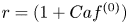 $r = (1+Ca f^{(0)})$ as,
 \begin{align} \left. \begin{aligned} (\boldsymbol{u}|_{r= (1+Ca f^{(0)})})^{(1)}=\boldsymbol{u}^{(1)}|_{r=1}+ f^{(0)} \boldsymbol{\nabla} \boldsymbol{u}^{(0)} \boldsymbol{\cdot} \boldsymbol{x}|_{r=1} ,\\ (\boldsymbol{\sigma} \boldsymbol{\cdot} \boldsymbol{n} )^{(1)}_{r= (1+Ca f^{(0)})} =\boldsymbol{\sigma}^{(1)}|_{r=1} \boldsymbol{\cdot} \boldsymbol{n}^{(0)}+\boldsymbol{\sigma}^{(0)}|_{r=1} \boldsymbol{\cdot} \boldsymbol{n}^{(1)} + f^{(0)}( \boldsymbol{\nabla} \boldsymbol{\sigma}^{(0)} \boldsymbol{\cdot} \boldsymbol{x}|_{r=1} ) \boldsymbol{\cdot} \boldsymbol{n}^{(0)}. \end{aligned} \right\} \end{align}
From (2.9), (2.10) and (3.16), we obtain the normal vector  $\boldsymbol{n}^{(1)}$ and the curvature of the interface $(\boldsymbol {\nabla } \boldsymbol{\,\cdot\, n})^{(2)}$ at ${O}(Ca)$ as
 \begin{equation} \boldsymbol{n}^{(1)}={-}\boldsymbol{\nabla} f^{(0)}=2b_{1}\left(\frac{\boldsymbol{x}(\boldsymbol{x}\boldsymbol{\cdot} \boldsymbol{\mathsf{E}} \boldsymbol{\cdot} \boldsymbol{x} )}{r^{4}}-\frac{\boldsymbol{\mathsf{E}} \boldsymbol{\cdot} \boldsymbol{x}}{r^{2}} \right)_{r=1}, \end{equation}
and
 \begin{align} (\boldsymbol{\nabla}
\boldsymbol{\,\cdot\, n})^{(2)}&= 2((f^{(0)})^{2}-f^{(1)})-(
\nabla^{2} f)^{(1)}-(\boldsymbol{\nabla} f^{(0)} )^{2}
-\boldsymbol{x \,\cdot\,}( \boldsymbol{\nabla} f^{(0)}
\boldsymbol{\cdot} \boldsymbol{\nabla} \boldsymbol{\nabla}
f^{(0)} ) \nonumber\\ &=({-}10b_{1}^{2}+18b_{5})(
\boldsymbol{x} \boldsymbol{\cdot} \boldsymbol{\mathsf{E}} \boldsymbol{\cdot} \boldsymbol{x} )^{2}+4b_{2} \boldsymbol{x}
\boldsymbol{\cdot} \boldsymbol{\mathsf{E}} \boldsymbol{\cdot} \boldsymbol{x} -(2b_3+2b_4) \boldsymbol{\mathsf{E}} \boldsymbol{:}\boldsymbol{\mathsf{E}}
\nonumber\\ &\quad + (4b_{4}-8b_{5}) \boldsymbol{x \,\cdot }
(\boldsymbol{\mathsf{E}} \boldsymbol{\cdot} \boldsymbol{\mathsf{E}})\boldsymbol{ \cdot\, x}+\,4b_{6}
\boldsymbol{x \,\cdot } (\boldsymbol{\varOmega}\boldsymbol{\cdot}\boldsymbol{\mathsf{E}})\boldsymbol{ \cdot\,
x}\,-(2b_{7}+2b_{8})\boldsymbol{\varOmega : \varOmega}
\nonumber\\ &\quad +4b_{8} \boldsymbol{x \,\cdot }
(\boldsymbol{\varOmega \cdot \varOmega})\boldsymbol{ \,\cdot \,
x}, \end{align}
\begin{align} (\boldsymbol{\nabla}
\boldsymbol{\,\cdot\, n})^{(2)}&= 2((f^{(0)})^{2}-f^{(1)})-(
\nabla^{2} f)^{(1)}-(\boldsymbol{\nabla} f^{(0)} )^{2}
-\boldsymbol{x \,\cdot\,}( \boldsymbol{\nabla} f^{(0)}
\boldsymbol{\cdot} \boldsymbol{\nabla} \boldsymbol{\nabla}
f^{(0)} ) \nonumber\\ &=({-}10b_{1}^{2}+18b_{5})(
\boldsymbol{x} \boldsymbol{\cdot} \boldsymbol{\mathsf{E}} \boldsymbol{\cdot} \boldsymbol{x} )^{2}+4b_{2} \boldsymbol{x}
\boldsymbol{\cdot} \boldsymbol{\mathsf{E}} \boldsymbol{\cdot} \boldsymbol{x} -(2b_3+2b_4) \boldsymbol{\mathsf{E}} \boldsymbol{:}\boldsymbol{\mathsf{E}}
\nonumber\\ &\quad + (4b_{4}-8b_{5}) \boldsymbol{x \,\cdot }
(\boldsymbol{\mathsf{E}} \boldsymbol{\cdot} \boldsymbol{\mathsf{E}})\boldsymbol{ \cdot\, x}+\,4b_{6}
\boldsymbol{x \,\cdot } (\boldsymbol{\varOmega}\boldsymbol{\cdot}\boldsymbol{\mathsf{E}})\boldsymbol{ \cdot\,
x}\,-(2b_{7}+2b_{8})\boldsymbol{\varOmega : \varOmega}
\nonumber\\ &\quad +4b_{8} \boldsymbol{x \,\cdot }
(\boldsymbol{\varOmega \cdot \varOmega})\boldsymbol{ \,\cdot \,
x}, \end{align}
respectively. The system of equations obtained by imposing the boundary conditions are given in Appendix B. In the limit  $\alpha \to \infty$, the expressions for the constants (refer (B16)–(B30) in Appendix B) are consistent with the ${O}(Ca)$ calculations for a drop (Ramachandran & Leal Reference Ramachandran and Leal2012). As done earlier, the kinematic boundary condition may be used to evaluate the shape function, $f^{(1)}$ as,
 \begin{equation} \frac{\partial f^{(1)}}{\partial t}=(\boldsymbol{u} \boldsymbol{\,\cdot\, n})^{(1)}_{r=(1+Ca f^{(0)})}, \end{equation}
which further reduces to the description of temporal evolution of the deformed interface as,
 \begin{gather} \frac{\partial b_{2}}{\partial t}=\frac{c_{4}}{2 }+ 9c_{12} , \end{gather}
 \begin{gather}\frac{\partial b_{4}}{\partial t}={-}\frac{3c_{5}}{2 }- 24c_{6} + 9c_{16} - 300c_{23} -b_{1}(2- 12c_{3} ), \end{gather}
 \begin{gather}\frac{\partial b_{5}}{\partial t}=\frac{75c_{6}}{2 }+ 525c_{23} +b_{1}(3-c_{1} - 48c_{3} ), \end{gather}
 \begin{gather}\frac{\partial b_{6}}{\partial t}={-}\frac{3c_{8}}{2 }- 6c_{20} -9c_{25} +2b_{1}, \end{gather}
 \begin{gather}\frac{\partial b_{8}}{\partial t}={-}\frac{3c_{9}}{2 }-9c_{24}. \end{gather}
Here, the variables  $c_i$ are linear functions of $b_j$ where $j$ varies from $2$ to $8$. We solve the above set of (3.25a)–(3.25e) along with (3.19a,b) to obtain the shape parameters $b_{j}$. The temporal evolution of the shape is illustrated using plots in the next section and the steady state shape values of $b_{j}$ are given in Appendix C. The expressions for the shape functions in the limit $\alpha \to \infty$ are also given in Appendix C (refer (C2)–(C7)), they are consistent with the calculations for a drop (Ramachandran & Leal Reference Ramachandran and Leal2012).
Hence, using a domain perturbation approach and standard technique of superposition of vector harmonics, we calculated the pressure and velocity fields up to  ${O}(Ca)$ in both inner and outer fluids for a compound particle when subjected to an imposed linear flow. Along with these, we determined the time evolution of the deforming interface of the confining drop up to ${O}(Ca^2)$. These solutions are illustrated in the next section for various linear flows.
4. Deformation dynamics of a compound particle in a general linear flow
In the previous section, we described the  ${O}(1)$ flow field (Chaithanya & Thampi Reference Chaithanya and Thampi2019), and then derived the ${O}(Ca)$ flow field generated by a compound particle and the corresponding consequences, namely the ${O}(Ca)$ and ${O}(Ca^2)$ corrections to the confining drop shape. We now analyse these results for different linear flows (i) a simple shear flow, and (ii) extensional (both uniaxial and biaxial) flows. We then expand the discussion on interface deformation dynamics for generalised shear and generalised extensional flows in this section.
4.1. Simple shear flow
Consider a simple shear flow of the form  $\boldsymbol{u}= x_{2} \boldsymbol {i}_{1}$, where $x_{2}$ is the component of position vector $\boldsymbol{x}$ and $i_{1}$ is the unit normal vector associated with $x_{1}$ in the chosen coordinate system. The symmetric and anti-symmetric parts of the velocity gradient tensor of the imposed flow are,
 \begin{equation} \boldsymbol{\mathsf{E}}^{S}=\frac{1}{2}\begin{bmatrix} 0 & 1 & 0 \\ 1 & 0 & 0\\ 0 & 0 & 0 \end{bmatrix}, \quad \boldsymbol{\varOmega}^{S}=\frac{1}{2}\begin{bmatrix} 0 & 1 & 0 \\ -1 & 0 & 0\\ 0 & 0 & 0 \end{bmatrix}. \end{equation}
Using (4.1a,b), the shape of the confining drop may be obtained as,
 \begin{align} r(\theta, \phi)&=\left(1+ b_{1} Ca\left(\frac{x_{1}x_{2}}{r^{2}} \right)+Ca^{2}\left(b_{2}\frac{x_{1}x_{2}}{r^{2}}+\frac{b_{3}-b_{7}}{2} +\frac{b_{4}-b_{8}}{4}\left(\frac{x_{1}^{2}+x_{2}^{2}}{r^{2}}\right) \right.\right.\nonumber\\ & \quad \left.\left.+b_{5}\frac{x_{1}^{2}x_{2}^{2}}{r^{4}}+\frac{b_{6}}{4} \left(\frac{x_{1}^{2}-x_{2}^{2}}{r^{2}}\right)\right)+O(Ca^3)\right), \end{align}
where  $x_{1}=r\sin {\theta }\cos {\phi }$, $x_{2}=r\sin {\theta }\sin {\phi }$ and $x_{3}=r\cos {\theta }$, $r$ is the magnitude of the position vector $\boldsymbol{x}$, $\theta$ is the polar angle measured from the $x_{3}$ axis ( $0\leq \theta \leq {\rm \pi}$) and $\phi$ is the azimuthal angle measured around the $x_3$ axis ( $0 \leq \phi \leq 2{\rm \pi}$).
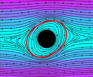
The steady state flow fields in and around a deformed compound particle are illustrated in figure 2(a). Equations (A2), (A4), (B2), (B4) and (C1) have been used to calculate the velocity field and the corresponding confining drop shape. For comparison,  ${O}(1)$ velocity field is shown in figure 2(b) (Chaithanya & Thampi Reference Chaithanya and Thampi2019). In the imposed simple shear flow, the encapsulated rigid particle rotates with an angular velocity $\mathcal {G}/2$, and the curved streamlines inside the confining drop illustrate the recirculating fluid flow around this rotating rigid particle. Similarly, the outer fluid close to the interface also has curved streamlines. However, compared to that of a spherical compound particle (figure 2b) or a particle without a confining drop (Sadhal et al. Reference Sadhal, Ayyaswamy and Chung1997; Leal Reference Leal2007), the streamlines around the compound particle show distortions corresponding to the deformed interface.

Figure 2. (a) Velocity field, represented as streamlines, in and around a compound particle in an imposed shear flow in the flow–gradient ( $x_{1}$– $x_{2}$) plane, for $\alpha =2$, $Ca=0.1$ and $\lambda =1$. The ${O}(1)$ flow field is shown in (b) for comparison. The colour field shows the magnitude of velocity. The filled circle is the encapsulated solid particle and the solid red line shows the confining drop interface.
Now we proceed to analyse the confining drop shape and its evolution. The time evolution of the confining drop shape (up to  ${O}(Ca^{2})$) in a simple shear flow for $\alpha =2$, $\lambda =1$ and $Ca=0.2$ is depicted in figure 3(a). At $t=0$, the confining drop is spherical, but the imposed flow deforms the interface with time. Finally, the confining drop attains a steady shape that is elongated in a direction close to the extensional axis of the imposed flow and compressed in the orthogonal direction.

Figure 3. The time evolution of (a) the confining drop shape in a simple shear flow for  $\lambda =1$, $\alpha =2$ and $Ca=0.2$ (equations (3.6), (3.25) along with (3.19a,b)). The black patch at the centre indicates the encapsulated solid particle. (b) The deformation parameter $\mathcal {D}$ determined by (4.3), and (c) the alignment angle $\varphi$, for various size ratios $\alpha$ and viscosity ratios $\lambda$. The solid lines correspond to $\mathcal {D}$ (and $\varphi$) obtained for various $\alpha$ and the dotted lines correspond to those obtained for various $\lambda$.
Similar to the deformation parameter defined by Taylor (Reference Taylor1932) to analyse the shape of drops, we define a deformation parameter  $\mathcal {D}$ as
 \begin{equation} \mathcal{D}=\frac{(r_{max}- a)-(r_{min}-a)}{(r_{max}-a)+(r_{min}-a)}, \end{equation}
that quantifies the extent of deformation of the compound particle as done in Chaithanya & Thampi (Reference Chaithanya and Thampi2019). Here,  $r_{max}$ and $r_{min}$ are the longest and shortest dimensions of the deformed interface as shown in figure 1. The limits, $\mathcal {D}=0$ and $\mathcal {D}=1$ respectively correspond to the case of an undeformed spherical interface and the case where the confining interface touches the encapsulated solid particle. The latter case can be regarded as the onset of break-up of the confining drop since the interface comes into contact with the encapsulated solid particle. Therefore, unlike that of a simple drop, large values of deformation parameter do not necessarily mean a large deformation of the confining drop. This is especially the case in the limit $\alpha \to 1$. In other words, in the limit $\alpha \to 1$, breakup ( $\mathcal {D} = 1$) may occur even with a weak deformation of the confining drop, and therefore the perturbation approach used in this work remains valid all the way up to the confining drop breakup.
The time evolution of deformation parameter  $\mathcal {D}$ for $Ca=0.2$ but for various values of $\alpha$ and $\lambda$ are plotted in figure 3(b). In all cases, $\mathcal {D}$ increases with time indicating the progression of deformation. Finally $\mathcal {D}$ reaches a plateau corresponding to the steady state shape of the confining drop. In some cases, $\mathcal {D}$ reaches $1$ representing the break up of the confining interface. Of course the progression of deformation and the final value of $\mathcal {D}$ depend upon the particular values of $\alpha$ and $\lambda$, and this dependence is discussed later in this section.
Another consequence of calculations at  ${O}(Ca^2)$ is its ability to predict the orientation of the elongated interface in a simple shear flow. The ${O}(Ca)$ correction to the confining drop shape shows that the elongated direction of the confining drop aligns with the extensional axis of the flow, i.e. $45^\circ$ with the flow direction in the flow–gradient plane as reported in Chaithanya & Thampi (Reference Chaithanya and Thampi2019). However, ${O}(Ca^2)$ calculation takes into account the effect of vorticity of the imposed flow, which then predicts that the elongated interface does not orient along the extensional axis of the imposed flow. We define an alignment angle $\varphi$, as shown in figure 1, as the angle between the elongated direction of the confining drop and the flow direction ( $x_1$) in a simple shear flow.
The time evolution of alignment angle  $\varphi$ at $Ca=0.2$ for various values of $\alpha$ and $\lambda$ is plotted in figure 3(c). The alignment angle $\varphi$ decreases with time before reaching a steady value, indicating that the deformed drop rotates towards the flow direction as dictated by the imposed vorticity, finally attaining an orientation that is in between the flow direction and the extensional axis of the imposed shear flow.
The extent of deformation of the confining interface of the compound particle that resulted from the imposed shear flow is different in different directions. The steady state shape of the confining drop (see (4.2)), when viewed in three different planes, namely the flow–gradient ( $x_{1}$– $x_{2}$), flow–vorticity ( $x_{1}$– $x_{3}$) and gradient–vorticity ( $x_{2}$– $x_{3}$) planes are shown in figures 4(a)–4(c). The interface deformation is largest in the flow–gradient plane with the confining drop elongated in a direction described by $\varphi$. Confining drop is lesser deformed in the flow–vorticity plane and the gradient–vorticity plane, with the interface elongated in the flow direction in the former and compressed along the vorticity direction in the latter.

Figure 4. The deformed shape (see (4.2)) of the confining drop viewed from various planes: (a) in flow–gradient ( $x_{1}$– $x_{2}$) plane, (b) in flow–vorticity ( $x_{1}$– $x_{3}$) plane and (c) in gradient–vorticity ( $x_{2}$– $x_{3}$) plane for different capillary numbers. The dashed line represents the initial, undeformed shape of the confining drop and the filled circle is the encapsulated solid particle.
Figures 4(a)–4(c) also illustrate the deformed shape of the confining drop for various capillary numbers. Increase in  $Ca$ signifies increasingly dominant shear force over the resisting interfacial tension and, therefore, the extent of deformation of the confining interface increases with increase in $Ca$. This is evident from the confining drop shapes shown in various planes (figures 4(a)–4(c)). For the largest capillary number $Ca = 0.3$ considered in this figure, dimples form on the interface, as evident in the flow–gradient plane (figure 4a). The extent of compression of the interface is not same in all directions, with the maximum compression observed along the vorticity direction. Incidentally, in this particular case, the deformed interface comes in contact with the encapsulated solid particle (figure 4c) and marks the break up of the confining drop.
The extent of deformation of the confining drop is mainly dependent upon the three non-dimensional numbers, namely the capillary number  $Ca$, the size ratio $\alpha$ and the viscosity ratio $\lambda$, as illustrated comprehensively in figure 5. The steady state deformation parameter $\mathcal {D}$ as a function of $Ca$ for various $\alpha$ and $\lambda$ is shown in figures 5(a) and 5(b) respectively. The corresponding steady state shapes of the deformed interface of the compound particle at a fixed $Ca =0.1$ but for various $\alpha$ and $\lambda$ are shown in figures 5(c) and 5(d) respectively. The deformation parameter (or deformation of the confining drop) increases with increase in capillary number $Ca$, and decreases with increase in size ratio $\alpha$ and viscosity ratio $\lambda$. This dependency of steady state deformation parameter on $Ca$,
$Ca$,  $\alpha$ and $\lambda$ based on leading-order calculations is reported by Chaithanya & Thampi (Reference Chaithanya and Thampi2019), and they are shown as dotted lines in figure 5. The $O(Ca^2)$ calculations are shown as solid lines in figure 5.

Figure 5. The effect of  $Ca$ on the steady state deformation parameter $\mathcal {D}$ (a) for various size ratios $\alpha$, at $\lambda =1$ and (b) for various viscosity ratios $\lambda$, at $\alpha =1.5$. The markers in (a, b) indicate $Ca_{crit}$, the capillary number at which $D = 1$, which signifies breakup of the confining drop as the interface comes in contact with the encapsulated rigid particle. The corresponding steady state confining drop shapes at $Ca=0.1$ and (c) for various $\alpha$ and (d) for various $\lambda$. The solid and the dotted lines correspond to ${O}(Ca^2)$ and ${O}(Ca)$ calculations respectively.
As expected  ${O}(Ca)$ and ${O}(Ca^2)$ theory respectively show a linear and a quadratic dependence of $\mathcal {D}$ on $Ca$. More importantly, ${O}(Ca)$ calculations underpredict the deformation parameter. (However, at very large viscosity ratios, ${O}(Ca)$ calculations overpredict the value of $\mathcal {D}$.) Interestingly, the difference between ${O}(Ca^2)$ and ${O}(Ca)$ calculations decreases with decrease in $\alpha$, and with increase in $\lambda$ at a fixed capillary number. This is because, small $\alpha$ or large $\lambda$ correspond to cases where the deformed interface of the confining drop deviates least from the spherical shape. The degree of underprediction in $\mathcal {D}$ by linear theory is proportional to $Ca$, showing that ${O}(Ca^2)$ theory significantly deviates from ${O}(Ca)$ predictions as capillary number increases. This observation also assumes importance because, compared to ${O}(Ca^2)$ calculations the linear theory will also be overpredicting $Ca_{crit}$, the capillary number at which break up of the confining interface of the compound particle occurs.
Similar to  $\mathcal {D}$, the alignment angle also depends upon the capillary number, the size ratio and the viscosity ratio. Figures 6(a) and 6(b) show the dependency of steady state $\varphi$ on $Ca$ for various size ratios and viscosity ratios. In all cases, the alignment angle decreases with increase in $Ca$, making the elongated interface to orient closer to the flow direction of the imposed shear flow. The vorticity associated with the imposed flow acts to rotate the deformed drop towards the flow axis, while the surface tension force acts to revert it back to the spherical shape, and this competition determines the alignment angle. If the surface tension forces dominate the shear forces (smaller $Ca$), the confining drop aligns with the extensional axis, otherwise the confining drop aligns more with the flow axis. Similarly, $\varphi$ decreases with decrease in $\alpha$ or $\lambda$ at a given $Ca$. Thus, the deformed drop aligns closer to the flow axis in strong shear flows, and when the encapsulated particle is bigger and the viscosity of the confining fluid is larger. This behaviour of alignment angle following that of deformation parameter occurs as larger deformation results in more anisotropic shapes that orient closer to the flow direction.

Figure 6. The effect of capillary number on the steady state alignment angle,  $\varphi$ calculated from (4.2) in a simple shear flow (a) for various size ratios at $\lambda = 1$ and (b) for various viscosity ratios at $\alpha = 1.5$.
To summarise this section, we have analysed fluid flows in and around a compound particle as well as the consequent deformation of the confining interface when it is subjected to an imposed shear flow. The  ${O}(Ca^2)$ calculation of the deformed shape of the confining drop shows that the deformation of the interface increases with increase in $Ca$ and this larger deformation results in orienting the deformed interface to align close to the flow axis in a simple shear flow. Further, the steady state deformation parameter and the critical capillary number increase while the alignment angle decreases with increase in $\alpha$ and $\lambda$ due to increased hydrodynamic interaction between the enclosed solid and the confining interface.
4.2. Extensional flows
In this section, we analyse the deformation of the confining drop when the compound particle is subjected to an extensional flow. This analysis is important since earlier investigations, both experimental (Taylor Reference Taylor1934; Bai Chin & Dae Han Reference Bai Chin and Dae Han1979; Grace Reference Grace1982; Mietus et al. Reference Mietus, Matar, Lawrence and Briscoe2002; Mulligan & Rothstein Reference Mulligan and Rothstein2011) and theoretical or numerical (Taylor Reference Taylor1934; Bai Chin & Dae Han Reference Bai Chin and Dae Han1979; Qu & Wang Reference Qu and Wang2012), have concluded that the deformation and breakup of a simple drop (without encapsulated particles) differ considerably when subjected to shear and extensional flows.
Consider the two extensional flows namely, the uniaxial and biaxial flows described by the strain rate tensor,
 \begin{equation} \boldsymbol{\mathsf{E}}^{E}=\frac{1}{2}\begin{bmatrix} \mp1 & 0 & 0 \\ 0 & \mp1 & 0\\ 0 & 0 & \pm2 \end{bmatrix}, \quad \boldsymbol{\varOmega}^{E}=\boldsymbol{0}, \end{equation}
where the first and second signs indicate uniaxial and biaxial flows, respectively. We follow the same convention throughout this section. Then the shape of the confining drop for uniaxial and biaxial flows can be obtained as
 \begin{align} r(\theta, \phi)&= \left( 1+b_{1} Ca \left({\mp}\frac{1}{2}\frac{(x_{1}^{2}+x_{2}^{2})}{r^{2}} \pm\frac{x_{3}^{2}}{r^{2}}\right)+Ca^{2}\left(b_{2}\left({\mp} \frac{1}{2}\frac{(x_{1}^{2}+x_{2}^{2})}{r^{2}}\pm\frac{x_{3}^{2}}{r^{2}}\right)\right.\right.\nonumber\\ &\quad +\left.\left.\frac{3}{2}b_{3} +b_{4} \left(\frac{1}{4}\frac{(x_{1}^{2}+x_{2}^{2})}{r^{2}} +\frac{x_{3}^{2}}{r^{2}}\right) +b_{5} \left(\frac{1}{2}\frac{(x_{1}^{2}+x_{2}^{2})}{r^{2}} -\frac{x_{3}^{2}}{r^{2}}\right)^{2}\right)+O(Ca^3) \right). \end{align}
 Figures 7(a) and 7(b) show the velocity fields in and around a compound particle obtained for uniaxial and biaxial flows, respectively. The deformed shape of the confining drop is also plotted (solid red line). Clearly, the velocity fields are similar in both cases with recirculating fluid flows appearing in each quadrant. The orientation of the elongated interface is along the extensional axis of the flow but the extent of the deformation is different for uniaxial and biaxial flows. For uniaxial flows, extensional axis of the imposed flow is along the  $x_3$ axis while for biaxial flows extensional flow is in the radial direction in the $x_1\text {--}x_2$ plane. This difference results in the confining interface adopting a prolate spheroid-like shape for uniaxial flows and an oblate spheroid-like shape for biaxial flows. These shapes, for various $\alpha$, when viewed in two different planes, the $x_1\text {--}x_3$ plane and the $x_1\text {--}x_2$ plane are shown in figures 7(c)–7(f). The axisymmetry of the deformed shapes is apparent in the $x_1\text {--}x_2$ plane in all cases.

Figure 7. Velocity field in and around a compound particle in an imposed (a) uniaxial and (b) biaxial flow. Here,  $\alpha =2$, $Ca=0.1$ and $\lambda =1$. The colour bar represents the magnitude of the velocity. Effect of the size ratio $\alpha$ on the deformation of a compound particle (c) in the $x_{1}$– $x_{3}$ plane and (e) in the $x_{1}$– $x_{2}$ plane for uniaxial flow and (d) in the $x_{1}$– $x_{3}$ plane and (f) in the $x_{1}$– $x_{2}$ plane for biaxial flow. The solid and dotted lines represent the drop shape at ${O}(Ca^2)$ and ${O}(Ca)$ (Chaithanya & Thampi Reference Chaithanya and Thampi2019) respectively.
As earlier, the deformation parameter  $\mathcal {D}$ can also be calculated using (4.3) for uniaxial and biaxial flows as
 \begin{equation} \mathcal{D}=\frac{3\alpha}{4(\alpha-1)}\left( b_{1} Ca+Ca^{2}\left(b_{2}\pm\frac{b_{4}}{2}\pm\frac{b_{5}}{2}\mp\frac{\alpha b_{1}^{2}}{4(\alpha-1)} \right) \right) +O(Ca^3). \end{equation}
In the limit of  $\lambda \rightarrow \infty$ and ( $\alpha - 1) \rightarrow 0$ such that the hydrodynamic interaction between the encapsulated particle and the interface is a dominant effect, (4.6) reduces to give the deformation parameter as,
 \begin{equation} \mathcal{D}= \frac{630\alpha(\alpha-1)Ca\pm\alpha(671\alpha-986)Ca^{2}}{420 (\alpha-1)^2}. \end{equation}
Thus,  $\mathcal {D}$ is same for uniaxial and biaxial flows up to ${O}(Ca)$ but differ at ${O}(Ca^2)$. This difference is also illustrated in figures 7(c)–7(f). The deformation calculated at ${O}(Ca^2)$ (solid lines) is more compared to that at ${O}(Ca)$ (dotted lines) for uniaxial flows. On the other hand, for biaxial flows, drop deformation and thus the predicted value $\mathcal {D}$ are less at ${O}(Ca^2)$ compared to that at ${O}(Ca)$. In other words, ${O}(Ca)$ calculation underpredicts deformation for uniaxial flows and overpredicts it for biaxial flows.
Similar to the case of a simple shear flow, the deformation of a confining drop in extensional flows increases with decreasing  $\alpha$ or $\lambda$ for a particular $Ca$, and increases with increase in $Ca$. These dependencies can also be understood by monitoring critical capillary number, $Ca_{crit}$ beyond which the confining drop breaks up ( $\mathcal {D} = 1$). Therefore, $Ca_{crit}$ is plotted as a function of $\lambda$ for various $\alpha$ and various imposed flows in figure 8. Irrespective of the flow type, $Ca_{crit}$ increases with increase in $\lambda$ or $\alpha$. For small viscosity ratios, $\lambda <1$, $Ca_{crit}$ for shear flows is smaller suggesting that shear flows are stronger in deforming the interface compared to the uniaxial and biaxial flows. This trend reverses for large $\lambda$. As mentioned earlier, due to the difference in the deformation characteristics, uniaxial flows show lower $Ca_{crit}$ compared to biaxial flows.

Figure 8. The variation of the critical capillary number  $Ca_{crit}$ vs the viscosity ratio $\lambda$ for various size ratios $\alpha ~(=1.5, 2, 2.5)$ and in different imposed flows.
4.3. Generalised shear and extensional flows
In this section, we expand the analysis described in the two previous sections to generalised shear and generalised extensional flows. We may define a generalised shear flow (Graham Reference Graham2018) which has the velocity gradient tensor as,
 \begin{equation} \boldsymbol{\mathsf{E}}^{GS}=\frac{(1+\beta)}{2}\begin{bmatrix} 0 & 1 & 0 \\ 1 & 0 & 0\\ 0 & 0 & 0 \end{bmatrix}, \quad \boldsymbol{\varOmega}^{GS}=\frac{(1-\beta)}{2}\begin{bmatrix} 0 & 1 & 0 \\ -1 & 0 & 0\\ 0 & 0 & 0 \end{bmatrix},\end{equation}
where the parameter  $\beta$ takes values from $-1$ to $1$. The limiting cases of $\beta =-1$ and $\beta =1$ correspond to the pure rotational and pure straining flows, respectively. Simple shear flow is obtained when $\beta = 0$.
Figure 9 shows the steady state flow fields in and around a deformed compound particle for  $\beta = -1$ and $\beta = 1$. As shown in figure 9(a), for $\beta = -1$ which corresponds to a pure rotational flow, the velocity field has only azimuthal component of velocity, there will not be any velocity normal to the interface, and therefore the confining drop remains spherical. As $\beta$ increases, the strength of the extensional component in the imposed flow increases (refer to figure 9b), which results in larger deformations, with the largest $D$ obtained for a purely extensional flow ( $\beta = 1$).

Figure 9. Velocity field in and around a compound particle in an imposed flow; (a)  $\beta =-1$, (b) $\beta =1$. Here, $\alpha =2$, $Ca=0.05$ and $\lambda =1$. The colour bar represents the magnitude of the velocity.
Figure 10(a) summarises the deformation behaviour of the confining drop of the compound particle by plotting the dependence of deformation parameter,  $\mathcal {D}$, on $\beta$. In purely rotational flows ( $\beta = -1$), the confining drop does not deform ( $\mathcal {D} = 0$), since the imposed flow corresponds to deformation free (rigid-body-like) rotation of the fluid. As $\beta$ increases, the strength of extensional component in the imposed flow increases which results in larger deformations, with largest $\mathcal {D}$ obtained for $\beta =1$. Figure 10(a) also shows the predicted values of $\mathcal {D}$ at ${O}(Ca)$, shown as dotted lines for comparison. In the linear theory, $\mathcal {D}$ increases linearly with $\beta$ with rotational component playing no role. As mentioned earlier, the first effect of imposed vorticity is taken into account at ${O}(Ca^{2})$, and thus $\mathcal {D}$ calculated at ${O}(Ca^{2})$ exhibits a nonlinear behaviour with an increase in $\beta$, as shown. Thus, in the rotation dominated flows ( $\beta < 1$), ${O}(Ca)$ calculation underpredicts the deformation of the confining drop. On the other hand, as $\beta \rightarrow 1$, ${O}(Ca)$ overpredicts $\mathcal {D}$. It is also worth noting that ${O}(Ca^{2})$ corrections are significant when the hydrodynamic interaction between the encapsulated particle and the confining drop interface becomes strong. Therefore, the case of $\alpha = 1.5$ shows largest deviation in the predicted values of $\mathcal {D}$ at ${O}(Ca^2)$ compared to predictions of linear theory.

Figure 10. The deformation parameter  $\mathcal {D}$ (a) in generalised shear flows, as a function of $\beta$ and (b) in generalised extensional flows as a function of $m$. In these plots, $\lambda =1$ and $Ca=0.1$. Solid and dotted lines correspond to ${O}(Ca^2)$ and ${O}(Ca)$ calculations.
A similar analysis can be performed for extensional flows as well, where the generalised extensional flow may be defined with a velocity gradient tensor as,
 \begin{equation} \boldsymbol{\mathsf{E}}^{GE}=\frac{1 }{\sqrt{2(1+m+m^2)}}\begin{bmatrix} 1 & 0 & 0 \\ 0 & m & 0\\ 0 & 0 & -(1+m) \end{bmatrix}, \quad \boldsymbol{\varOmega}^{GE} = \boldsymbol{0},\end{equation}
where, the parameter  $m$ may take different values. For example, $m = -1/2$ corresponds to a uniaxial flow ( $x_1$ being the extensional axis), $m =0$ corresponds to a planar extensional flow and $m =1$ corresponds to a biaxial flow ( $x_3$ being the compressional axis).
Figure 10(b) shows the dependency of deformation parameter  $\mathcal {D}$ on $m$. Clearly, the deformation parameter is only weakly dependent on $m$, with $\mathcal {D}$ varying only slightly between uniaxial ( $m = -1/2$), planar extensional ( $m = 0$) and biaxial ( $m = 1$) flows. However, irrespective of the type of imposed flow, $\mathcal {D}$ increases with decrease in $\alpha$. Again, predictions from ${O}(Ca)$ calculations are shown as dotted lines in the same figure for comparison. It is interesting to note that, the linear theory shows a monotonic increase of $\mathcal {D}$ with $m$ while this is not the case at ${O}(Ca^2)$. The implication is that linear theory falsely suggests that biaxial flows ( $m = 1$) are stronger than uniaxial flows ( $m = -1/2$) in deforming the confining interface (Chaithanya & Thampi Reference Chaithanya and Thampi2019), while the situation reverses by taking into account of ${O}(Ca^2)$ corrections. In other words, $\mathcal {D}$ at $m = 1$ is smaller than $\mathcal {D}$ at $m = -1/2$, similar to the calculations for a simple drop (Davis & Brenner Reference Davis and Brenner1981), and therefore, uniaxial flows are stronger in deforming a compound particle. This effect may be understood as follows. Biaxial flow compresses the confining drop towards an oblate shape while a uniaxial flow stretches it towards a prolate shape. As deformation increases, the prolate shaped interface meets the solid inclusion before the corresponding oblate. Therefore, though biaxial flow is obtained by reversing the direction of uniaxial flow, the latter is stronger than the former to cause breakup of the confining drop. The other observation to note is that, as observed for generalised shear flows, the difference that arises due to ${O}(Ca^2)$ corrections from the linear theory also increases with decrease in $\alpha$, making the ${O}(Ca^2)$ calculations more relevant for compound particles.
5. Rheology of a dilute dispersion of compound particles
So far, we have analysed the deformation dynamics of a compound particle when subjected to various imposed flows using the results derived from a domain perturbation approach. The same analysis is useful in predicting the rheological behaviour of a suspension of compound particles. In this section, we characterise the rheology of a dilute dispersion of compound particles in terms of effective shear viscosity, extensional viscosity, normal stress differences and the complex modulus.
Consider a dispersion made up of compound particles such as those shown in figure 1 (encapsulated particle of size  $a$, confining interface of size $b = a\alpha$ and inner fluid viscosity $\hat {\mu }$) in a carrier fluid of viscosity $\mu = \lambda \hat {\mu }$. The volume fraction (based on the size of the confining drop) of the compound particles $\phi \ll 1$, so that the dispersion is dilute and hence any hydrodynamic interaction between the compound particles will be neglected. On subjecting this dispersion to an imposed flow described by a rate of strain tensor $\boldsymbol{\mathsf{E}}$, we may define a volume-averaged stress (Batchelor Reference Batchelor1970) for the dispersion as,
 \begin{equation} \langle \boldsymbol{\sigma}\rangle={-}\langle p \rangle \boldsymbol{\mathsf{I}}+2 \boldsymbol{\mathsf{E}}+ \phi \boldsymbol{\mathsf{S}}, \end{equation}
where  $\boldsymbol{\mathsf{S}}$ is the stresslet associated with a single compound particle. This quantity can be easily extracted from the steady state far field solution of the disturbance velocity field generated by a single compound particle (calculated in §§ 3.1 and 3.2),
 \begin{align} \boldsymbol{u} = \left(-\frac{c_{1}}{6} \boldsymbol{\mathsf{E}}+Ca \left(\frac{c_{5}}{2}(\boldsymbol{\mathsf{E}} \boldsymbol{\cdot} \boldsymbol{\mathsf{E}} -\frac{\boldsymbol{\mathsf{I}}}{3}(\boldsymbol{\mathsf{E}} \boldsymbol{:}\boldsymbol{\mathsf{E}})) +\frac{c_{8}}{4}(\boldsymbol{\varOmega}\boldsymbol{\cdot}\boldsymbol{\mathsf{E}}-\boldsymbol{\mathsf{E}}\boldsymbol{\cdot}\boldsymbol{\varOmega}) \right) \right)\boldsymbol{:} \left(\frac{\boldsymbol{\mathsf{I}}\boldsymbol{x}}{r^{3}}-\frac{3\boldsymbol{x x x}}{r^{5}}\right), \end{align}
where the last bracketed term  $({\boldsymbol{\mathsf{I}} \boldsymbol{x}}/{r^{3}}-{3\boldsymbol{x x x}}/{r^{5}})$ is the symmetric part of the gradient of Oseen tensor. The expression for $c_{1}$ is given in Appendix A (see (A5)), and the expressions for $c_{5}$ and $c_{8}$ are given in Appendix B (see (B14) and (B15)). Therefore, as implied by the boundary integral equations for creeping flow, the stresslet can be identified as (Batchelor Reference Batchelor1970; Leal Reference Leal2007; Ramachandran & Leal Reference Ramachandran and Leal2012),
 \begin{equation} \boldsymbol{\mathsf{S}} = 8 {\rm \pi}\left(-\frac{c_{1}}{6} \boldsymbol{\mathsf{E}}+Ca \left(\frac{c_{5}}{2}\left(\boldsymbol{\mathsf{E}} \boldsymbol{\cdot} \boldsymbol{\mathsf{E}} -\frac{\boldsymbol{\mathsf{I}}}{3}(\boldsymbol{\mathsf{E}} \boldsymbol{:}\boldsymbol{\mathsf{E}})\right) +\frac{c_{8}}{4}(\boldsymbol{\varOmega}\boldsymbol{\cdot}\boldsymbol{\mathsf{E}}-\boldsymbol{\mathsf{E}}\boldsymbol{\cdot}\boldsymbol{\varOmega}) \right) \right). \end{equation}
Substituting (5.3) in to (5.1) gives an expression for the volume-averaged stress as,
 \begin{align} \langle\boldsymbol{\sigma}\rangle&={-}\langle p \rangle\boldsymbol{\mathsf{I}}+2 \boldsymbol{\mathsf{E}}\left(1- \phi \frac{c_{1}}{2 } \right) +\phi Ca \left( 3c_{5} \left(\boldsymbol{\mathsf{E}} \boldsymbol{\cdot} \boldsymbol{\mathsf{E}} -\frac{\boldsymbol{\mathsf{I}}}{3}(\boldsymbol{\mathsf{E}} \boldsymbol{:}\boldsymbol{\mathsf{E}}) \right)\right.\nonumber\\ &\left.\quad +\,\frac{3c_{8}}{2 }( \boldsymbol{\varOmega}\boldsymbol{\cdot}\boldsymbol{\mathsf{E}}-\boldsymbol{\mathsf{E}}\boldsymbol{\cdot}\boldsymbol{\varOmega})\right)+{O}(\phi^{2}, \phi^2 Ca, \phi Ca^2), \end{align}
which can be further analysed to extract the rheological quantities of interest for a dilute dispersion of compound particles as discussed below.
5.1. Shear viscosity
Subjecting the dilute dispersion of compound particles to an imposed flow,  $\boldsymbol{u}^{imp}= x_{2} \boldsymbol {i}_{1}$, the effective shear viscosity of the dispersion can be calculated from (5.4) as,
 \begin{equation} \mu_{eff}= \frac{\langle\sigma\rangle_{12}}{2E_{12}} = \left(1-\phi \frac{c_{1} }{2} \right)+{O}(\phi^{2}, \phi^2 Ca, \phi Ca^2 ). \end{equation}
Thus, the first correction to the shear viscosity is  ${O}(\phi )$ and it depends only on the leading-order stress field. In other words, ${O}(Ca)$ stress field generated due to deformation of the confining drop does not contribute to shear viscosity for dilute dispersions. However, hydrodynamic interaction between compound particles can lead to further corrections, which will be accounted at ${O}(\phi ^2)$. Taking appropriate limits the expression derived above for shear viscosity (5.5) can also be deduced from the works of Davis & Brenner (Reference Davis and Brenner1981), Stone & Leal (Reference Stone and Leal1990), Mandal et al. (Reference Mandal, Ghosh and Chakraborty2016) and Das et al. (Reference Das, Mandal and Chakraborty2020).
It is interesting to look at the limiting case of (5.5) first. (i) In the limit,  $\alpha \rightarrow 1$ (or $\lambda \rightarrow 0$), (5.5) reduces to the Einstein relation for the effective viscosity of a dilute suspension of spherical rigid particles $\mu _{eff} = (1+\frac {5 }{2} \phi )$ (Einstein Reference Einstein1906, Reference Einstein1911). (ii) In the limit of $\alpha \rightarrow \infty$, (5.5) reduces to Taylor's relation for the effective viscosity of a dilute emulsion $\mu _{eff} = (1+ (({5+2\lambda })/({2+2\lambda }))\phi )$ (Taylor Reference Taylor1932; Oldroyd Reference Oldroyd1953). (iii) In the limit of $\alpha \to 1$, but retaining ${O}(\alpha - 1)$ terms, the effective shear viscosity of a suspension of particles that are coated with a thin fluid film of inner fluid can be calculated as,
 \begin{equation} \mu_{eff} \simeq \left(1+\phi \left( \tfrac{5}{2}-\tfrac{15}{8} (\alpha-1) \lambda+{O}(\alpha-1)^{2} \right) \right). \end{equation}
Therefore,  ${O}(\alpha -1)$ correction to the effective viscosity of a dispersion is negative, indicating that the viscosity of a dilute suspension of spheres can be reduced by providing a thin coating of a viscous fluid. (iv) In the limit of $\lambda \rightarrow \infty$, (5.5) reduces to the effective viscosity of a dilute emulsion of bubbles $\mu _{eff} = (1+ \phi )$, where the positive viscosity correction arises purely due to the interfacial tension of the confining interface.
Figure 11(a) shows the complete picture, where the enhancement factor in the effective shear viscosity  $(\mu _{eff}-1)/\phi$ is plotted as a function of size ratio $\alpha$ and viscosity ratio $\lambda$. At a given viscosity ratio, $\mu _{eff}$ decreases with increase in $\alpha$ from Einstein's to Taylor's limit. Similarly, for a given size ratio, the effective viscosity decreases with increase in viscosity ratio. This behaviour can be understood as follows. As the resistance to the fluid flow increases, an increase in the effective viscosity may be anticipated. The resistance to the imposed flow is maximum in the case of rigid solid spheres. This resistance decreases with increase in the thickness of the coating (confining drop size) on the rigid spheres. Therefore, the effective viscosity decreases with increase in the size of the confining drop ( $\alpha$). Similarly, as the viscosity of the inner fluid decreases, the resistance to the imposed flow decreases, thus, the outer fluid can easily slip past the confining interface. Therefore, the effective viscosity decreases with increase in the viscosity ratio. It is worth noting that, as mentioned earlier, $Ca$ does not appear at ${O}(\phi )$ in (5.4) and therefore the stress resulting from the deformation of the confining drop does not have any effect on these calculations.


Another useful rheological measure that can be extracted from (5.4) is the shear viscosity of the compound particles when the confining interface has zero surface tension or  $Ca\rightarrow \infty$. This corresponds to a situation where the kinematic boundary condition (2.8) is not respected, $b_{1} = 0$ and therefore the effective shear viscosity is obtained as,
 \begin{equation} \mu_{eff}^{S}= \left(1-\frac{\phi c_{1}^{S}}{2}\right), \end{equation}
where the expression for  $c_{1}^{S}$ is given in Appendix A (see (A16)). In the limit of $\alpha \rightarrow \infty$, the $\mu _{eff}^{S} = \lambda \mu (1+\phi ({5(1-\lambda )}/{(2+3\lambda )}))$, a result obtained by Batchelor & Green (Reference Batchelor and Green1972) for a dilute emulsion of drops.
Figure 11(b) illustrates the dependence of  $\mu _{eff}^{S}$ on the size ratio and viscosity ratio of the compound particles in the dispersion. The dependence of $\mu _{eff}^{S}$ on $\alpha$ and $\lambda$ is similar to that of $\mu _{eff}$, however, with the important difference that the effective viscosity $\mu _{eff}^{S}$ is smaller than the suspending fluid viscosity $\mu$ for a range of viscosity ratios. As seen in the figure, this reduction in viscosity occurs only beyond a viscosity ratio termed as critical viscosity ratio $\lambda _{c}^{S}$. Equating $\mu _{eff}^{S}-1$ to zero, we obtain the critical viscosity ratio from (5.7) as,
 \begin{align} \lambda_{c}^{S}&={-}(3 \alpha^{10}+125 \alpha^7-336 \alpha^5+200 \alpha^3+8 -5 (49 \alpha^{20}+14 \alpha^{17}-1175 \alpha^{14}+2352 \alpha^{12}\nonumber\\ &\quad -1288 \alpha^{10}-16 \alpha^7+64)^{1/2})/(8 (4 \alpha^{10}-25 \alpha^7+42 \alpha^5-25 \alpha^3+4)), \end{align}
beyond which a reduction in viscosity will be observed.
5.2. Extensional viscosity
By subjecting the dilute dispersion of compound particles to a uniaxial extensional flow, we can calculate the extensional viscosity (or Trouton's viscosity)  $\mu _{eff}^{T}$ as the ratio of the normal stress difference to the imposed shear rate,
 \begin{equation} \mu_{eff}^{T}=\frac{\sigma_{33}-\sigma_{11}}{E_{33}}=\frac{\sigma_{33}-\sigma_{22}}{E_{33}}. \end{equation}
Hence, the extensional viscosity of a dilute dispersion of compound particles can be obtained from (5.4) as
 \begin{equation} \mu_{eff}^{T}= \left(3+3\phi\left(-\frac{c_{1}}{2 }+Ca\frac{3c_{5}}{4 } \right)\right)+{O}(\phi^{2}, \phi^{2} Ca, \phi Ca^2 ). \end{equation}
The above expression (5.10) can be deduced from the work of Santra et al. (Reference Santra, Panigrahi, Das and Chakraborty2020b) on compound drops by taking the appropriate limit.
The dependencies of the Trouton viscosity of a dilute dispersion of compound particles on the size ratio and viscosity ratio of individual compound particles are shown in figure 12. Again, instead of viscosity, it is the enhancement factor  $(\mu _{eff}^{T}-3\mu _{eff})/\phi$ that is plotted against $\lambda$. For a Newtonian fluid, the Trouton viscosity is equal to $3\mu _{eff}$ and the enhancement factor is exactly zero. This limit is indicated by the flat line in figure 12. Dispersions of compound particles show deviations from this Newtonian limit – larger deviations (and thus larger $\mu _{eff}^{T}$) are observed for smaller values of $\alpha$ and $\lambda$. As $\lambda$ increases, the enhancement factor for the Trouton viscosity asymptotes to a constant, independent of $\alpha$. On the other hand, for a given $\lambda$, increase in $\alpha$ reduces the Trouton viscosity. The decrease in the Trouton viscosity with an increase in the size ratio or with an increase in the viscosity ratio occurs for the same reason as the decrease in the effective viscosity discussed in the previous section.

Figure 12. The variation of the Trouton viscosity vs the viscosity ratio  $\lambda$ for various size ratios and $Ca=0.1$.
These observations can also be endowed by analysing (5.10). The Newtonian limit can be recovered for the special case, when  $Ca = 0$ so that the confining interface is exactly spherical, and (5.10) reduces to give the extensional viscosity $\mu _{eff}^{T} = 3\mu _{eff}$. In general, compound particles show deviations from this Newtonian behaviour since $Ca \neq 0$ and the confining drop is deformed. Of course, as mentioned in the previous sections, the extent of the deviation depends upon the specific values of $\alpha$ and $\lambda$. For large values of $\lambda$ the enhancement factor $(\mu _{eff}^{T}-3\mu _{eff})/\phi$ asymptotes to ${36 Ca}/{35}$ a constant, which is independent of $\alpha$ and consistent with the observations in figure 12. In the limit of $\alpha \to 1$, but retaining ${O}(\alpha - 1)$ terms, the extensional viscosity of a suspension of particles that are coated with a thin fluid film of inner fluid can be calculated as,
 \begin{equation} \frac{\mu_{eff}^{T}-3\mu_{eff}}{\phi} \simeq Ca \left( -\frac{675 (\lambda-4)}{896 (\alpha-1)}+\frac{225 (45 \lambda^2-130 \lambda+136)}{3584}+{O}(\alpha-1) \right). \end{equation}
It is clear that the Trouton viscosity increases with a decrease in  $\alpha$. In the opposite limit, the case of simple drops without encapsulated particles, i.e. as $\alpha \rightarrow \infty$, (5.10) provides the enhancement factor $(\mu _{eff}^{T}-3\mu _{eff})/\phi = 9 Ca (64 \lambda ^3+732 \lambda ^2+1179 \lambda +475)/ (560 (\lambda +1)^3)$. This result matches with the result of Ramachandran & Leal (Reference Ramachandran and Leal2012) with the slip coefficient being zero and with Mandal et al. (Reference Mandal, Das and Chakraborty2017) when no surfactants are present.
Hence, it is clear that a larger Trouton viscosity is observed for smaller values of  $\alpha$ and $\lambda$. This behaviour is qualitatively similar to that of the effective shear viscosity. However, comparison with the case of $Ca = 0$ suggests that deviations from the Newtonian limit ( $\mu _{eff}^T \neq 3\mu _{eff}$) arise in the dispersion of compound particles due to the deformation of the confining interface. Consequently, a time-dependent increase in the deformation of the confining drop (as discussed in § 4.1) can give rise to a time-dependent increase in the extensional viscosity. Another feature to notice is that, (5.11) shows that the enhancement factor for $\mu _{eff}^{T}$ of a dilute dispersion of compound particles can be made negative. This is similar to the case of shear viscosity and indicates that the extensional viscosity of a dilute suspension of spheres can be reduced by providing a thin film coating of a less viscous fluid on the particles.
5.3. Normal stress differences
In § 4, we have seen that an imposed flow acts to deform the confining spherical drop while the interfacial tension acts to revert it back, yielding an anisotropic shape of the confining drop. Therefore, the force distribution around the compound particle will also be anisotropic, inducing normal stress differences in a dispersion of compound particles. Normal stress differences, a characteristic of viscoelastic behaviour of a fluid, can also be determined by analysing the volume-averaged stress (5.4) as in the last two sections.
Subjecting the dilute dispersion of compound particles to a simple shear flow  $\boldsymbol{u}^{imp}= x_{2} \boldsymbol {i}_{1}$, (5.4) renders the first and second normal stress differences $N_{1}$ and $N_{2}$ as
 \begin{gather} N_{1}=\sigma_{11}-\sigma_{22}=\phi Ca \left(\frac{3c_{8}}{2}\right)+{O}(\phi^{2}, \phi^{2}Ca, \phi Ca^2 ) , \end{gather}
 \begin{gather}N_{2}=\sigma_{22}-\sigma_{33}=\phi Ca \left(\frac{3(c_{5}-c_{8})}{4}\right)+{O}(\phi^{2}, \phi^{2}Ca, \phi Ca^2 ). \end{gather}
 The dependency of the first and second normal stress differences on the viscosity and size ratio of compound particles is shown in figure 13(a). In all cases,  $N_1$ is positive and $N_2$ is negative. Moreover, it may be noted that both $N_{1}$ and $-N_{2}$ decrease with an increase in the viscosity ratio for a given $\alpha$. The asymptotic values of the normal stresses as $\lambda \rightarrow \infty$ can be deduced from (5.12) and (5.13) respectively as $N_{1}/\phi Ca=32/5$ and $-N_{2}/\phi Ca = 20/7$. For a given viscosity ratio, both $N_1$ and $-N_2$ decrease with an increase in the size ratio. The two data sets are put together in figure 13(b), which shows the ratio of normal stress differences, $-N_{2}/N_{1}$ as a function of $\lambda$ for various $\alpha$. This ratio increases with an increase in $\lambda$ or $\alpha$. Irrespective of $\alpha$ and $\lambda$, the value of $\mod {-N_2/N_1}$ is less than $1$. This behaviour can be understood by analysing the extent of deformation of the confining drop in different planes. We have seen that the deformation of the confining drop is larger in the flow–gradient plane compared to that in the vorticity–gradient plane. Therefore, the $N_1$ which is based on the stresses in the flow–gradient plane is always larger than the $N_2$ which is based on the stresses in the vorticity–gradient plane. The maximum value of $-N_{2}/N_{1} = 0.4464$ is approached at large $\lambda$, independent of the value of $\alpha$.

Figure 13. Effect of the viscosity ratio  $\lambda$ on the normal stress differences for different size ratios; (a) $N_{1}/\phi Ca$ (solid lines) and $N_{2}/\phi Ca$ (dash-dotted lines), (b) $-N_{2}/N_{1}$.
The limiting case of  $\alpha \rightarrow \infty$ which corresponds to a dilute suspension of drops that does not contain encapsulated particles, is also shown in figure 13(a). The mathematical expressions that correspond to these curves can be obtained from (5.12) and (5.13) respectively, as $N_{1}/\phi Ca = (16 \lambda +19)^2 / (40 (\lambda +1)^2)$ and $N_{2}/\phi Ca = -(800 \lambda ^3+1926 \lambda ^2+1623 \lambda +551 )/(280 (\lambda +1)^3 )$, and they are consistent with the works of Ramachandran & Leal (Reference Ramachandran and Leal2012) and Mandal et al. (Reference Mandal, Das and Chakraborty2017). On the other hand, in the limit $\alpha \rightarrow 1$, which corresponds to solid particles coated with a thin film of inner fluid, we can determine the normal stress differences as
 \begin{equation} \frac{N_{1}}{\phi Ca}=\frac{45}{32 (\alpha-1)^2} -\frac{15 (15 \lambda-34)}{64 (\alpha-1)}+\frac{ (3375 \lambda^2-5460 \lambda+4412)}{512}+{O}(\alpha-1), \end{equation}
and
 \begin{align} \frac{N_{2}}{\phi Ca}={-}\frac{45}{64 (\alpha-1)^2}+\frac{15 (45 \lambda-89)}{448 (\alpha-1)} -\frac{16875 \lambda^2-18720 \lambda+10484}{7168}+{O}(\alpha-1). \end{align}
The apparent large increase in  $N_1$ and $-N_2$ as $\alpha \rightarrow 1$ represents the result of increased deformation of the confining interface in this limit. These expressions hold correct only when $Ca < Ca_{crit}$, i.e. when the thin film coated on the particle is stable (without breakup) in the imposed flow.
Hence, as observed for the extensional viscosity, both  $N_1$ and $N_2$ are also dependent upon extent of deformation of the confining drop. Consequently, the normal stress differences for a dilute dispersion of compound particles will exhibit capillary-number-dependent and time-dependent behaviour following the extent of deformation of the confining interface.
5.4. Small-amplitude oscillatory shear flow
Finally, we characterise the linear viscoelastic behaviour of a dilute dispersion of compound particles by subjecting the dispersion to a SAOS. In general, the rheological response of the dispersion may be linear or nonlinear, and the transition from linear to nonlinear response can be observed by increasing the amplitude of the shear rate at a fixed frequency. In the following, we restrict our analysis to the linear regime, where the analytical calculations are possible.
Consider an imposed oscillatory shear flow of the form
 \begin{equation} \boldsymbol{u}^{imp}= \exp{(\textrm{i}\omega t)} x_{2} \boldsymbol{i}_{1}, \end{equation}
where  $\omega$ is the frequency of oscillation. In the linear regime, shear stress is related to the complex modulus ( $G^*$) (Ramachandran & Leal Reference Ramachandran and Leal2012) via,
 \begin{equation} \langle \sigma_{12}\rangle= \frac{G^{*}}{\omega} 2E_{12}, \end{equation}
where  $G^{*}=G^{\prime }+ \textrm {i} \omega G^{\prime \prime }$, $G^{\prime }$ is the elastic or storage modulus and $G^{\prime \prime }$ is the viscous or loss modulus. Comparing (5.17) and the volume-averaged stress, (5.4), we find that
 \begin{equation} G^{*}=\omega\left(1-\phi \frac{c_1}{2}\right). \end{equation}
The constant  $c_1$ in (5.18), associated with the velocity field, is dependent on the drop shape parameter $b_1$.
Previously, in § 4.1, we described the time evolution  $b_1$, and thus the shape of the confining interface in an imposed simple shear flow. Here, we need to analyse the time evolution of the shape parameter $b_{1}$ in an imposed oscillatory shear flow, which is obtained from the leading-order kinematic boundary condition, (2.11), as
 \begin{equation} \frac{\partial b_{1}}{\partial t}+\textrm{i} \omega b_{1}={-}\frac{b_{1}-b_{1}^{*}}{t_{c}}. \end{equation}
In the long time limit, where the unsteady term can be neglected, so that we can obtain a frequency-dependent shape parameter,
 \begin{equation} b_{1}=\frac{b_{1}^{*}}{1+\textrm{i} \omega t_{c}}. \end{equation}
Following the procedure developed in Ramachandran & Leal (Reference Ramachandran and Leal2012), we evaluate  $c_{1}$ in terms of $b_{1}$ using (5.20) and substitute it in (5.18), to obtain the expression for the complex modulus ( $G^*$) as,
 \begin{align}
G^{\prime}+\textrm{i} \omega G^{\prime \prime} &=\omega
\left(1-\frac{\phi }{2}\right.(5(( (40- 100 \alpha^3 + 100
\alpha^7 - 40 \alpha^{10} )\lambda - 4 (\alpha-1)^4 (4 + 16
\alpha\nonumber\\ &\quad + 40 \alpha^2 + 55 \alpha^3 + 40
\alpha^4 + 16 \alpha^5 + 4 \alpha^6 ) \lambda^2)+
\textrm{i} \omega ({-}48 - 200 \alpha^3 + 336 \alpha^5\nonumber\\ &\quad -
225 \alpha^7 - 38 \alpha^{10} + (16 +
400 \alpha^3 - 672 \alpha^5 + 250 \alpha^7 + 6 \alpha^{10}
)\lambda\nonumber\\ &\quad + 8 ({-}1 + \alpha)^4 (4 + 16 \alpha + 40 \alpha^2 + 55 \alpha^3 + 40 \alpha^4 + 16
\alpha^5 + 4 \alpha^6 ) \lambda^2 ) ) /\nonumber\\ &\quad ( ({-}40 + 100
\alpha^3 - 100 \alpha^7 + 40 \alpha^{10} ) \lambda
+10 ({-}1 + \alpha)^4 (4 + 16 \alpha + 40
\alpha^2\nonumber\\ & \quad + 55 \alpha^3+ 40 \alpha^4 + 16 \alpha^5 + 4
\alpha^6 ) \lambda^2 + \textrm{i} \omega (48 + 200 \alpha^3 - 336 \alpha^5 + 225 \alpha^7\nonumber\\ & \quad + 38
\alpha^{10}+ (- 96+ 100 \alpha^3 - 168 \alpha^5 +75
\alpha^7+ 89 \alpha^{10} ) \lambda +12 ({-}1
+ \alpha)^4\nonumber\\ &\quad
\left. \vphantom{\frac{\phi }{2}}
\times (4 + 16 \alpha + 40 \alpha^2 + 55 \alpha^3 + 40
\alpha^4 + 16 \alpha^5 + 4 \alpha^6 ) \lambda^2 ) ) )\right).
\end{align}
\begin{align}
G^{\prime}+\textrm{i} \omega G^{\prime \prime} &=\omega
\left(1-\frac{\phi }{2}\right.(5(( (40- 100 \alpha^3 + 100
\alpha^7 - 40 \alpha^{10} )\lambda - 4 (\alpha-1)^4 (4 + 16
\alpha\nonumber\\ &\quad + 40 \alpha^2 + 55 \alpha^3 + 40
\alpha^4 + 16 \alpha^5 + 4 \alpha^6 ) \lambda^2)+
\textrm{i} \omega ({-}48 - 200 \alpha^3 + 336 \alpha^5\nonumber\\ &\quad -
225 \alpha^7 - 38 \alpha^{10} + (16 +
400 \alpha^3 - 672 \alpha^5 + 250 \alpha^7 + 6 \alpha^{10}
)\lambda\nonumber\\ &\quad + 8 ({-}1 + \alpha)^4 (4 + 16 \alpha + 40 \alpha^2 + 55 \alpha^3 + 40 \alpha^4 + 16
\alpha^5 + 4 \alpha^6 ) \lambda^2 ) ) /\nonumber\\ &\quad ( ({-}40 + 100
\alpha^3 - 100 \alpha^7 + 40 \alpha^{10} ) \lambda
+10 ({-}1 + \alpha)^4 (4 + 16 \alpha + 40
\alpha^2\nonumber\\ & \quad + 55 \alpha^3+ 40 \alpha^4 + 16 \alpha^5 + 4
\alpha^6 ) \lambda^2 + \textrm{i} \omega (48 + 200 \alpha^3 - 336 \alpha^5 + 225 \alpha^7\nonumber\\ & \quad + 38
\alpha^{10}+ (- 96+ 100 \alpha^3 - 168 \alpha^5 +75
\alpha^7+ 89 \alpha^{10} ) \lambda +12 ({-}1
+ \alpha)^4\nonumber\\ &\quad
\left. \vphantom{\frac{\phi }{2}}
\times (4 + 16 \alpha + 40 \alpha^2 + 55 \alpha^3 + 40
\alpha^4 + 16 \alpha^5 + 4 \alpha^6 ) \lambda^2 ) ) )\right).
\end{align}
In the limit of  $\alpha \rightarrow \infty$, which corresponds to a drop without a suspended particle, the complex modulus is given as
 \begin{equation} G^{\prime}+\textrm{i} \omega G^{\prime \prime}=\omega \left(1+ 5\phi \frac{4 \lambda (5+ 2 \lambda )+ \textrm{i} \omega (19 - 3\lambda - 16 \lambda^2 )}{ 40 \lambda(1 +\lambda ) + \textrm{i} \omega ( 38 + 89 \lambda +48 \lambda^2 ) } \right), \end{equation}
and this matches with the expressions derived in Ramachandran & Leal (Reference Ramachandran and Leal2012).
Figure 14 shows the variation of the storage ( $G^{\prime }$) and loss ( $G^{\prime \prime }$) moduli with frequency ( $\omega$) for different size and viscosity ratios. The value of the storage modulus $G^{\prime }$, which varies as $\omega ^2$, is close to zero at low frequencies, but it increases with an increase in frequency, eventually reaching a plateau at high frequencies. On the other hand, the loss modulus $G^{\prime \prime }$ varies as $\omega$ at low and high frequencies. Figure 14 shows that viscous modulus, represented as $G^{\prime \prime }-\omega$ decreases with increase in frequency. It may be noticed that, irrespective of the size or viscosity ratio, the viscous modulus ( $G^{\prime \prime }$) dominates the elastic modulus ( $G^{\prime }$) at low frequencies and vice versa at high frequencies. In other words, at low frequencies, the viscous response dominates the elastic response and the dispersion behaves like a viscoelastic fluid. At high frequencies, the elastic response dominates the viscous response and thus the dispersion behaves like a viscoelastic solid. This difference in behaviour arises because, at low frequencies, the confining interface relaxes fast enough compared to the imposed time scale, i.e. $t_c < \omega ^{-1}$, leading to a fluid-like behaviour of the dilute dispersion. But at high frequencies, the interface does not relax fast enough to follow up with changes in the imposed flow that the dispersion of compound particles will show a history dependence. It can also be observed that, when $\alpha$ is sufficiently small, the viscous modulus dominates the elastic modulus irrespective of frequency. Therefore, a dilute suspension of spheres coated with a thin film always behaves like a viscoelastic fluid, provided $Ca\ll 1$. This analysis is valid only if (i) the time scale of the imposed flow ( $1/\omega$) is much larger than the momentum diffusion time scale ( $\rho a^2/\mu$) and (ii) the characteristic time scale of the droplet ( $t_c$) is much smaller than the characteristic time scale of the imposed flow ( $\omega ^{-1}$, $G^{-1}$). Mathematically, the above conditions are, $\rho a^2/\mu \ll \omega ^{-1}$, $t_c\ll \omega ^{-1}$ and $t_c \ll G^{-1}$. The first inequality is maintained by the choice of Reynolds number, while the second and third inequalities are maintained by carefully selecting the values of $\omega$, and $G^{-1}$.

Figure 14. The normalised components of the complex moduli  $G^{\prime }/\phi$ (solid lines) and $(G^{\prime \prime }-\omega )/\phi \omega$ (dash-dotted lines) vs the frequency $\omega$ (see (5.21)). Effects of (a) the size ratio $\alpha$ (for $\lambda =1$) and (b) the viscosity ratio $\lambda$ (for $\alpha =2$).
6. Conclusions
In this work, we analysed the deformation dynamics of a single compound particle when the encapsulated particle is concentrically located inside the confining drop. Assuming that the interface deformations are small, namely  $Ca\ll 1$ we solved the incompressible Stokes equations analytically using a domain perturbation approach and obtained the flow field correct up to $O(Ca)$ and the deformed shape of the confining interface up to $O(Ca^2)$. Using these results, we further characterised the rheology of a dilute dispersion of compound particles in terms of effective viscosities, normal stress differences and complex modulus.
On subjecting a compound particle to various linear flows it has been found that the presence of an encapsulated particle always enhances the deformation of the confining drop compared to a simple drop which does not contain an encapsulated particle. The enhanced deformation results from the hydrodynamic interaction between the encapsulated particle and the confining interface since the disturbance flow field developed inside the confining drop has to comply with the no-slip, no-penetration boundary conditions on the surface of the encapsulated particle and less stringent interfacial boundary conditions prescribing the continuity of velocity and stress on the confining interface. Naturally, decreasing the size of the encapsulated particle or decreasing the viscosity of the confining fluid will reduce the strength of the hydrodynamic interactions, thus resulting in less deformation of the confining interface. The extent of deformation of the confining interface was characterised by defining a deformation parameter, which also allowed us to calculate the critical capillary number  $Ca_{crit}$ at which the confining interface comes into contact with the encapsulated particle, resulting in a break up of the confining drop. Our analysis shows that $O(Ca^2)$ corrections to the drop shape are important and may qualitatively differ from the $O(Ca)$ predictions for compound particles. For example, $O(Ca)$ correction to the confining drop shape shows that the biaxial flow is stronger in deforming the confining interface compared to the uniaxial and shear flows at the same $Ca$. However, $O(Ca^2)$ correction shows that this is not true, instead either uniaxial or shear flows can be stronger depending upon the viscosity ratio of the confining fluid and the viscosity of the suspending medium. Similarly, in generalised extensional flows, the $O(Ca)$ correction shows a monotonic increase in deformation as we move from uniaxial to biaxial flows while the $O(Ca^2)$ correction shows a non-monotonic behaviour with deformation, being least for a biaxial flow. Another feature that emerges from $O(Ca^2)$ calculation is its ability to predict the reorientation dynamics of the anisotropically deformed interface. The elongated direction of the deformed interface rotates closer to the flow direction in an imposed simple shear flow. This reorientation can lead to a reduced deformation of the interface and, therefore, in the case of generalised shear flows, it was observed that deformation of the confining drop increases as we move from vorticity dominated flows to extension dominated flows. In other words, the deformation of the confining drop of a compound particle reduces either when the strength of vorticity increases or strength of extension reduces in the imposed flow.
Using the solution obtained from the domain perturbation approach, we have analysed the rheology of a dilute dispersion of compound particles. The different limits of the analysis, namely that of a dispersion of (i) solid particles, (ii) drops and (iii) solid particles coated with a thin fluid film have also been discussed in the context of each rheological quantity. The effective viscosity of a dilute dispersion of compound particles is found to vary between the effective viscosity of a dilute suspension of solid particles and fluid drops. While the effective viscosity is found to be independent of the drop deformation at  $O(Ca)$, it decreases with an increase in the size the confining drop or with a decrease in the viscosity of the inner fluid. For the special case of miscible fluids, the effective viscosity can be less than the suspending fluid viscosity in the limit of large viscosity ratio. Similar to the shear viscosity, the Trouton viscosity and normal stress differences decrease with increasing size of the confining drop or decreasing viscosity of the inner fluid (confining drop fluid). However, unlike the shear viscosity, these rheological parameters depend upon the extent of deformation of the confining interface and thus on $Ca$. It is interesting to note that, for very large viscosity ratios, these rheological parameters asymptote to a constant value that depends only on $Ca$ and not on the size ratio of the encapsulated particle to the confining interface.
The fact that the extensional viscosity is not equal to three times the shear viscosity indicates the non-Newtonian nature of a dilute dispersion of the compound particles, which was further characterised using a small-amplitude oscillatory shear flow. In the limit of low frequencies, we found that the viscous modulus dominates the elastic modulus since the confining interface relaxes to its quasi-steady state. However, at high frequencies, the interface deformation time scale is much smaller than the flow time scale that the elastic response dominates the viscous response. The viscous modulus is found to increase and the elastic modulus is found to decrease with a decrease in the size ratio of the confining drop to the particle. Similarly, we have shown that the viscous modulus increases and the elastic modulus decreases with a decrease in the viscosity ratio of the outer fluid to the inner fluid. The present study assumes that the surface tension force is much larger than the shear forces, that the capillary number is small and depends on a domain perturbation approach to proceed with analytical calculations. Numerical simulations will have to be employed to relax this assumption in order to go beyond the asymptotic limit of small capillary number and to quantitatively determine the deformation behaviour as well as rheology. Similarly, the consequences of eccentric configuration of the compound particle on the stability of the confining drop as well as rheology of the dispersion including hydrodynamic interactions between the compound particles also have to be the subject of future investigations. On the other hand, this study also inspires investigations related to active compound particles (the encapsulated particle is active, e.g. a microswimmer). Recently, Chaithanya & Thampi (Reference Chaithanya and Thampi2020) investigated the  $O(Ca)$ deformation dynamics of an active compound particle and discussed the interesting competition that arises from activity and the imposed flows. However, higher-order calculations, eccentric configurations and self-propulsion of active compound particles have to be the subject of future investigations.
Supplementary material
Supplementary material are available at https://doi.org/10.1017/jfm.2021.233.
Funding
S.P.T. acknowledges the support by Department of Science and Technology, India via the research grant CRG/2018/000644. P.K.S. acknowledges the support from IPDF grant by Indian Institute of Technology Madras, India.
Declaration of interests
The authors report no conflict of interest.
Appendix A
This appendix provides a complete description of the velocity and pressure fields of both inner and outer fluids at leading order ( ${O}(1)$) when subjected to a linear flow. The pressure and velocity fields for both outer and inner fluids at leading order, the same as (3.1)–(3.4) but simplified after substituting for the expressions for spherical harmonics, are as follows (Chaithanya & Thampi Reference Chaithanya and Thampi2019):
 \begin{gather}
p^{(0)}=\frac{c_{1}}{r^{5}}(\boldsymbol{x} \boldsymbol{\cdot}
\boldsymbol{\mathsf{E}} \boldsymbol{\cdot} \boldsymbol{x}),
\end{gather}
\begin{gather}
p^{(0)}=\frac{c_{1}}{r^{5}}(\boldsymbol{x} \boldsymbol{\cdot}
\boldsymbol{\mathsf{E}} \boldsymbol{\cdot} \boldsymbol{x}),
\end{gather}
 \begin{gather}\boldsymbol{u}^{(0)}=\left(1-\frac{6
c_{3}}{r^{5}}\right)\boldsymbol{\mathsf{E}}\boldsymbol{\cdot} \boldsymbol{x}+
\boldsymbol{\varOmega \cdot x} +
\left(\frac{c_{1}}{2r^{5}}+\frac{15
c_{3}}{r^{7}}\right)\boldsymbol{x} \boldsymbol{\cdot} (\boldsymbol{x} \boldsymbol{\cdot}
\boldsymbol{\mathsf{E}} \boldsymbol{\cdot} \boldsymbol{x}),
\end{gather}
\begin{gather}\boldsymbol{u}^{(0)}=\left(1-\frac{6
c_{3}}{r^{5}}\right)\boldsymbol{\mathsf{E}}\boldsymbol{\cdot} \boldsymbol{x}+
\boldsymbol{\varOmega \cdot x} +
\left(\frac{c_{1}}{2r^{5}}+\frac{15
c_{3}}{r^{7}}\right)\boldsymbol{x} \boldsymbol{\cdot} (\boldsymbol{x} \boldsymbol{\cdot}
\boldsymbol{\mathsf{E}} \boldsymbol{\cdot} \boldsymbol{x}),
\end{gather}
 \begin{gather}\hat{p}^{(0)}=\left(-\frac{126
d_{3}}{5}+\frac{e_{1}}{r^{5}}\right)(\boldsymbol{x} \boldsymbol{\cdot}
\boldsymbol{\mathsf{E}} \boldsymbol{\cdot} \boldsymbol{x}),
\end{gather}
\begin{gather}\hat{p}^{(0)}=\left(-\frac{126
d_{3}}{5}+\frac{e_{1}}{r^{5}}\right)(\boldsymbol{x} \boldsymbol{\cdot}
\boldsymbol{\mathsf{E}} \boldsymbol{\cdot} \boldsymbol{x}),
\end{gather}
 \begin{gather}\boldsymbol{\hat{u}}^{(0)}=\left(d_{2}-6
d_{3}r^{2}-\frac{6 e_{3}}{r^{5}} \right)
\boldsymbol{\mathsf{E}}\boldsymbol{\cdot} \boldsymbol{x}+ \boldsymbol{\varOmega
\cdot x} + \left( \frac{12 d_{3}}{5}+\frac{\lambda
e_{1}}{2r^{5}}+\frac{15 e_{3}}{r^{7}}\right)\boldsymbol{x}
\boldsymbol{\cdot} (\boldsymbol{x} \boldsymbol{\cdot} \boldsymbol{\mathsf{E}} \boldsymbol{\cdot} \boldsymbol{x}).
\end{gather}
\begin{gather}\boldsymbol{\hat{u}}^{(0)}=\left(d_{2}-6
d_{3}r^{2}-\frac{6 e_{3}}{r^{5}} \right)
\boldsymbol{\mathsf{E}}\boldsymbol{\cdot} \boldsymbol{x}+ \boldsymbol{\varOmega
\cdot x} + \left( \frac{12 d_{3}}{5}+\frac{\lambda
e_{1}}{2r^{5}}+\frac{15 e_{3}}{r^{7}}\right)\boldsymbol{x}
\boldsymbol{\cdot} (\boldsymbol{x} \boldsymbol{\cdot} \boldsymbol{\mathsf{E}} \boldsymbol{\cdot} \boldsymbol{x}).
\end{gather}
In (A1)–(A4), the unknown constants  $c_{i}$, $d_{i}$ and $e_{i}$ for $i=1,2,3$, are
 \begin{align} c_{1}&= ( ({-}240 -190 \alpha^{10}-1125 \alpha^7+1680 \alpha^5-1000 \alpha^3+ (30 \alpha^{10}+1250 \alpha^7-3360 \alpha^5\nonumber\\ &\quad +2000 \alpha^3+80 ) \lambda+ (160 \alpha^{10}-1000 \alpha^7+1680 \alpha^5-1000 \alpha^3+160 ) \lambda^2 )\nonumber\\ &\quad + b_{1} ( ({-}128 \alpha^{10}+800 \alpha^7-1344 \alpha^5+800 \alpha^3-128 ) \lambda^2\nonumber\\ &\quad + ({-}152 \alpha^{10}-100 \alpha^7+924 \alpha^5\nonumber\\ &\quad -800 \alpha^3+128 ) \lambda ) ) / ( 38 \alpha^{10}+225 \alpha^7-336 \alpha^5+200 \alpha^3+48 + (89 \alpha^{10}+75 \alpha^7\nonumber\\ &\quad-168 \alpha^5+100 \alpha^3 -96 ) \lambda+ (48 \alpha^{10}-300 \alpha^7+504 \alpha^5-300 \alpha^3+48 ) \lambda^2 ), \end{align}
 \begin{align} &\hspace{13pc}c_{2}=0,\end{align}
 \begin{align} c_{3}&= ( (48+ 38 \alpha^{10}+225 \alpha^7-336 \alpha^5+200 \alpha^3+ ({-}6 \alpha^{10}-425 \alpha^7+847 \alpha^5-400 \alpha^3\nonumber\\ &\quad -16 ) \lambda+ ({-}32 \alpha^{10}+200 \alpha^7-336 \alpha^5+200 \alpha^3-32 ) \lambda^2 )\nonumber\\ &\quad +b_{1} ( (16 \alpha^{10}-100 \alpha^7\!+\!168 \alpha^5 -100 \alpha^3+16 ) \lambda^2+ (24 \alpha^{10}+100 \alpha^7-308 \alpha^5\nonumber\\ &\quad +200 \alpha^3-16 ) \lambda ) )/ ( 6 (48 \alpha^{10}-300 \alpha^7 +504 \alpha^5-300 \alpha^3+48 ) \lambda^2\nonumber\\ &\quad+6 (89 \alpha^{10}+75 \alpha^7-168 \alpha^5+100 \alpha^3-96 ) \lambda+6 (38 \alpha^{10}\nonumber\\ &\quad +225 \alpha^7-336 \alpha^5+200 \alpha^3+48 ) ), \end{align}
 \begin{align} d_{1}&={-}126 ( ({-}250 \alpha ^5 (\alpha ^2-1 ) \!+\!250 \alpha ^5 (\alpha ^2-1 ) \lambda )-10 \alpha ^5 b_{1} (2 \alpha ^5-5 \alpha ^2+8\!+\! (3 \alpha^5 \!+\!5 \alpha ^2 \nonumber\\ &\quad -8 ) \lambda ) ) / 5 (3 (38 \alpha ^{10}+225 \alpha ^7-336 \alpha ^5+200 \alpha ^3+48 )+3 (89 \alpha ^{10}+75 \alpha ^7 -168 \alpha ^5\nonumber\\ &\quad +100 \alpha ^3 -96 ) \lambda +3 (48 \alpha ^{10} -300 \alpha ^7+504 \alpha ^5-300 \alpha ^3+48 ) \lambda ^2 ),\end{align}
 \begin{align} d_{2}&= (5 \alpha^3 \lambda ( 100+ 19 \alpha^7-84 \alpha^2+ (16 \alpha^7+84 \alpha^2-100 ) \lambda ) -4 \alpha^3 b_{1} \lambda ( 40+ 16 \alpha^7\nonumber\\ &\quad -21 \alpha^2+ (19 \alpha^7+21 \alpha^2-40 ) \lambda ) ) / ( 38 \alpha^{10}+225 \alpha^7-336 \alpha^5+200 \alpha^3 \nonumber\\ &\quad +48 + (89 \alpha^{10}+75 \alpha^7-168 \alpha^5+100 \alpha^3-96 ) \lambda + (48 \alpha^{10}-300 \alpha^7+504 \alpha^5\nonumber\\ &\quad -300 \alpha^3+48 ) \lambda^{2} ), \end{align}
 \begin{align} d_{3}&= ( ({-}250 \alpha ^5 (\alpha ^2-1 ) \lambda+250 \alpha^5 (\alpha ^2-1 ) \lambda ^2 )-10 \alpha ^5 b_{1} \lambda (2 \alpha ^5-5 \alpha ^2+8+ (3 \alpha^5\nonumber\\ &\quad +5 \alpha ^2-8 ) \lambda ) )/ (3 (38 \alpha ^{10}+225 \alpha ^7-336 \alpha ^5+200 \alpha ^3+48 )+3 (89 \alpha ^{10}+75 \alpha ^7\nonumber\\ &\quad -168 \alpha ^5+100 \alpha ^3-96 ) \lambda +3 (48 \alpha ^{10}-300 \alpha ^7+504 \alpha ^5-300 \alpha ^3+48 ) \lambda ^2 ),\end{align}
 \begin{align} e_{1}&= ({-}400-475 \alpha ^7+ (400-400 \alpha ^7 ) \lambda +b_{1} (320 \alpha ^7-168 \alpha ^5+128+ (380 \alpha ^7-252 \alpha ^5\nonumber\\ &\quad -128 ) \lambda ) )/ ( 38 \alpha ^{10}+225 \alpha ^7-336 \alpha ^5+200 \alpha ^3+48+ (48 \alpha ^{10} -300 \alpha ^7+504 \alpha ^5\nonumber\\ &\quad -300 \alpha ^3+48 ) \lambda ^2+ (89 \alpha ^{10}+75 \alpha ^7-168 \alpha ^5+100 \alpha ^3-96 ) \lambda +48 ), \end{align}
 \begin{align} e_{2}&= 0, \end{align}
 \begin{align} e_{3}&= (- ({-}95 \alpha ^5-80 ) \lambda - (80-80 \alpha ^5 ) \lambda ^2 +b_{1} (- (64 \alpha ^5 -40 \alpha ^3+16 ) \lambda - (76 \alpha ^5\nonumber\\ &\quad -60 \alpha ^3-16 ) \lambda ^2 ) ) / (6 (38 \alpha ^{10}+225 \alpha ^7-336 \alpha ^5+200 \alpha ^3+48 )+6 (89 \alpha ^{10}+75 \alpha ^7\nonumber\\ &\quad -168 \alpha ^5+100 \alpha ^3-96 ) \lambda + 6 (48 \alpha ^{10}-300 \alpha ^7+504 \alpha ^5-300 \alpha ^3+48 ) \lambda ^2 ). \end{align}
The  ${O}(1)$ velocity field also enabled the determination of the shape of the deformed interface of the confining drop up to ${O}(Ca)$. The deformed interface described in terms of the shape parameter $b_1=b_{1}^{*} (1-\exp (-{t}/{t_{c}}))$ (refer to (3.6)), where the time-independent parameter $b_{1}^{*}$ is
 \begin{align} b_{1}^{*} &= ({-}32 + 200 \alpha^3 - 231 \alpha^5 + 25 \alpha^7 + 38 \alpha^{10} + (32 - 200 \alpha^3 + 336 \alpha^5 - 200 \alpha^7 \nonumber\\ &\quad +32 \alpha^{10}) \lambda)/( 4 ({-}4 + 10 \alpha^3 - 10 \alpha^7 + 4 \alpha^{10}) \!+\! 4 (4 \!- 25 \alpha^3 \!+\! 42 \alpha^5 - 25 \alpha^7 + 4 \alpha^{10}) \lambda), \end{align}
and the time scale,  $t_{c}$, that controls the rate of deformation is
 \begin{align} t_{c}&=(48 + 200 \alpha^3 - 336 \alpha^5 + 225 \alpha^7 + 38 \alpha^{10} + ({-}96 + 100 \alpha^3 - 168 \alpha^5 + 75 \alpha^7 \nonumber\\ & \quad + 89 \alpha^{10}) \lambda + (48 - 300 \alpha^3 + 504 \alpha^5 - 300 \alpha^7 + 48 \alpha^{10}) \lambda^2 )/ (10 ({-}4 + 10 \alpha^3 \nonumber\\ &\quad - 10 \alpha^7 + 4 \alpha^{10}) \lambda + 10 (4 - 25 \alpha^3 + 42 \alpha^5 - 25 \alpha^7 + 4 \alpha^{10}) \lambda^2 ). \end{align}
When the confining interface has zero surface tension i.e.  $Ca \rightarrow \infty$ or $b_{1}=0$, the expression for $c_{1}$ simplifies to
 \begin{align} c_{1}^{S}&=5 ({-}38 \alpha^{10}-225 \alpha^7+336 \alpha^5-200 \alpha^3-48+ (6 \alpha^{10}+250 \alpha^7-672 \alpha^5 \nonumber\\ &\quad +400 \alpha^3+16 ) \lambda+ (32 \alpha^{10}-200 \alpha^7+336 \alpha^5-200 \alpha^3+32 ) \lambda^2 ) / (38 \alpha^{10} \nonumber\\ &\quad +225 \alpha^7-336 \alpha^5+200 \alpha^3+48+ (89 \alpha^{10}+75 \alpha^7-168 \alpha^5+100 \alpha^3-96 ) \lambda\nonumber\\ &\quad + (48 \alpha^{10}-300 \alpha^7+504 \alpha^5-300 \alpha^3+48 ) \lambda^2 ). \end{align}
The corresponding unknown constants for a drop (without an encapsulated particle) can be obtained by taking the limit  $\alpha \rightarrow \infty$, and are given by
 \begin{gather} c_{1}={-}\frac{2 \lambda+5}{\lambda+1}, \quad c_{2}=0, \quad c_{3}=\frac{1}{6 \lambda+6}, \end{gather}
 \begin{gather}d_{1}=\frac{21}{2(\lambda+1)}, \quad d_{2}={-}\frac{3 \lambda}{2 \lambda+2}, \quad d_{3}={-}\frac{5 \lambda}{12 (\lambda+1)}, \end{gather}
 \begin{gather}e_{1}=0, \quad e_{2}=0, \quad e_{3}=0. \end{gather}
Further, the steady state value of the shape parameter  $b_{1}$ for a simple drop is
 \begin{equation} b_{1}^{*}=\frac{16 \lambda+19}{8 (\lambda+1)}. \end{equation}
Appendix B
This appendix provides a complete description of the velocity and pressure fields of both inner and outer fluids at  ${O}(Ca)$ when subjected to a linear flow. The solutions, the same as (3.12)–(3.15) but simplified after substituting for the expressions for spherical harmonics, are as follows:
 \begin{align} p^{(1)}&=\left(\frac{c_{5}}{r^{3}}+\frac{6c_{6}}{r^{5}} \right)\boldsymbol{\mathsf{E}}\boldsymbol{:}\boldsymbol{\mathsf{E}}-\left( \frac{3c_{5}}{r^{5}}+\frac{60c_{6}}{r^{7}}\right)\boldsymbol{x \cdot (\boldsymbol{\mathsf{E}} \cdot \boldsymbol{\mathsf{E}}) \cdot x}+\frac{105c_{6}}{r^{9}}(\boldsymbol{x \cdot \boldsymbol{\mathsf{E}} \cdot x})^{2}\nonumber\\ &\quad -\frac{3c_{8}}{r^{5}} \boldsymbol{x \cdot (\varOmega \cdot \boldsymbol{\mathsf{E}}) \cdot x}, \end{align}
 \begin{align} \boldsymbol{u}^{(1)}&=\left(\frac{c_{5}}{2r^{3}}+\frac{3c_{6}}{r^{5}}-\frac{3c_{16}}{r^{5}} +\frac{30 c_{23}}{r^{7}} \right)\boldsymbol{x (\boldsymbol{\mathsf{E}}:\boldsymbol{\mathsf{E}})}+\left(\frac{6c_{6}}{r^{5}}-\frac{6c_{16}}{r^{5}}+\frac{120c_{23}}{r^{7}} \right)\boldsymbol{(\boldsymbol{\mathsf{E}} \cdot \boldsymbol{\mathsf{E}}) \cdot x} \nonumber\\ &\quad -\left( \frac{3c_{5}}{2r^{5}}+\frac{30c_{6}}{r^{7}}-\frac{15c_{16}}{r^{7}}+\frac{420c_{23}}{r^{9}}\right)\boldsymbol{x (x \cdot (\boldsymbol{\mathsf{E}} \cdot \boldsymbol{\mathsf{E}}) \cdot x)}\nonumber\\ &\quad -\left( \frac{15 c_{6}}{r^{7}}+\frac{420 c_{23}}{r^{9}} \right)\boldsymbol{(x \cdot \boldsymbol{\mathsf{E}}) (x\cdot \boldsymbol{\mathsf{E}} \cdot x)}+\left(\frac{105 c_{6}}{2r^{9}}+\frac{945 c_{23}}{r^{11}} \right)\boldsymbol{x (x \cdot \boldsymbol{\mathsf{E}} \cdot x)^{2}}\nonumber\\ &\quad +\left(\frac{3c_{25}}{r^{5}} \right)(\boldsymbol{\varOmega \cdot \boldsymbol{\mathsf{E}} }) \boldsymbol{\,\cdot\, x}-\left(\frac{3c_{25}}{r^{5}} \right)(\boldsymbol{\mathsf{E}}\boldsymbol{\cdot}\boldsymbol{\varOmega} ) \boldsymbol{\,\cdot\, x}-\left(\frac{3c_{8}}{2r^{5}}+\frac{15c_{25}}{r^{7}} \right)\boldsymbol{x (x \cdot (\varOmega \cdot \boldsymbol{\mathsf{E}}) \cdot x)},\end{align}
 \begin{align} \hat{p}^{(1)}&=\left(d_{5}r^{2}+6d_{6}r^{4}+d_{7}+\frac{e_{5}}{r^{3}}+\frac{6e_{6}}{r^{5}} \right)\boldsymbol{\mathsf{E}}\boldsymbol{:}\boldsymbol{\mathsf{E}}-\left(3d_{5}+60d_{6}r^{2}+\frac{3e_{5}}{r^{5}}\right.\nonumber\\ &\quad +\left.\frac{60e_{6}}{r^{7}}\right)\boldsymbol{x \cdot (\boldsymbol{\mathsf{E}} \cdot \boldsymbol{\mathsf{E}}) \cdot x}+\left(105d_{6} +\frac{105e_{6}}{r^{9}}\right)(\boldsymbol{x \cdot \boldsymbol{\mathsf{E}} \cdot x})^{2}\nonumber\\ &\quad -\left(3d_{8}+\frac{3e_{8}}{r^{5}} \right)\boldsymbol{x \cdot (\varOmega \cdot \boldsymbol{\mathsf{E}}) \cdot x}, \end{align}
 \begin{align} \boldsymbol{\hat{u}}^{(1)}&=\left(\frac{\lambda d_{5}r^2}{2}+\frac{\lambda d_{7}}{2}+d_{15}-3d_{16} r^{2}-\frac{120 d_{23} r^{4}}{7}+\frac{\lambda e_{5}}{2r^{3}}+\frac{3 \lambda e_{6}}{r^{5}}-\frac{3e_{16}}{r^{5}}\right.\nonumber\\ &\quad \left.+\frac{30 e_{23}}{r^{7}} \right)\boldsymbol{x (\boldsymbol{\mathsf{E}}:\boldsymbol{\mathsf{E}})} +\left(d_{13}-6d_{14} r^{2} -6 d_{16} r^{2} +120 d_{23} r^{4}+\frac{6 \lambda e_{6}}{r^{5}}-\frac{6e_{16}}{r^{5}}\right.\nonumber\\ &\quad \left.+\frac{120e_{23}}{r^{7}} \right)\boldsymbol{(\boldsymbol{\mathsf{E}} \cdot \boldsymbol{\mathsf{E}}) \cdot x}+\left( -\frac{3 \lambda d_{5}}{2}+15d_{16}+\frac{360 d_{23}r^{2}}{7}- \frac{3 \lambda e_{5}}{2r^{5}}-\frac{30 \lambda e_{6}}{r^{7}} \right.\nonumber\\ &\quad \left.+\frac{15e_{16}}{r^{7}} -\frac{420e_{23}}{r^{9}}\right)\boldsymbol{x (x \cdot (\boldsymbol{\mathsf{E}} \cdot \boldsymbol{\mathsf{E}}) \cdot x)}+\left(15 d_{14} -420d_{23}r^{2} -\frac{15 \lambda e_{6}}{r^{7}}\right.\nonumber\\ &\quad \left.-\frac{420 e_{23}}{r^{9}} \right)\boldsymbol{(x \cdot \boldsymbol{\mathsf{E}}) (x\cdot \boldsymbol{\mathsf{E}} \cdot x)}+\left(120d_{23}+\frac{105 \lambda e_{6}}{2r^{9}}+\frac{945 e_{23}}{r^{11}} \right)\boldsymbol{x (x \cdot \boldsymbol{\mathsf{E}} \cdot x)^{2}}\nonumber\\ &\quad +\left(d_{18}+3d_{25}r^{2} +\frac{3e_{25}}{r^{5}} \right)\boldsymbol{(\varOmega \cdot \boldsymbol{\mathsf{E}} ) \cdot x}+\left(d_{19}-3d_{25}r^{2}-\frac{3e_{25}}{r^{5}} \right)\boldsymbol{(\boldsymbol{\mathsf{E}} \cdot \varOmega ) \cdot x}\nonumber\\ &\quad -\left(\frac{3 \lambda d_{8}}{2}+15d_{25}+\frac{3 \lambda e_{8}}{2r^{5}}+\frac{15e_{25}}{r^{7}} \right)\boldsymbol{x (x \cdot (\varOmega \cdot \boldsymbol{\mathsf{E}}) \cdot x)}. \end{align}
The unknown constants are obtained on the application of boundary conditions as follows:
(i) The no-slip boundary condition (see (3.9)) on the surface of the particle gives the following set of equations:
(B5a)\begin{gather} -\frac{2\lambda d_{4} }{21 \alpha^{2} }+ \frac{ \lambda e_4 \alpha^{3}}{2} +15 e_{12}\alpha^5=0, \end{gather}(B5b)\begin{gather}d_{11}+\frac{5 \lambda d_{4}}{21 \alpha^{2}}- 6e_{12} \alpha^{5} =0, \end{gather}(B5c)\begin{gather} \frac{\lambda d_{5}}{2 \alpha^{2} }+\frac{\lambda d_{7}}{2}+d_{15}-\frac{3d_{16}}{\alpha^{2}}-\frac{120 d_{23} }{7 \alpha^{4} }+\frac{\lambda e_{5} \alpha^{3}}{2 }+ 3\lambda e_{6} \alpha^{5} +e_{15}\alpha^{3}\nonumber\\ \quad - 3e_{16}\alpha^{5}+ 30 e_{23} \alpha^{7}=0, \end{gather}(B5d)\begin{gather} d_{13}-\frac{6 d_{14}}{\alpha^{2}} -\frac{6 d_{16}}{\alpha^{2} }+\frac{120 d_{23}}{ \alpha^{4}}+6\lambda e_{6}\alpha^{5} - 6e_{16} \alpha^{5}+ 120 e_{23} \alpha^{7} =0, \end{gather}(B5e)\begin{gather}-\frac{3\lambda d_{5} }{2 \alpha^{2}}+\frac{15d_{16}}{\alpha^{2}}+\frac{360 d_{23}}{7 \alpha^{4}}-\frac{3 \lambda e_{5} \alpha^{3}}{2}- 30\lambda e_{6}\alpha^{5} + 15e_{16}\alpha^{5}- 420e_{23}\alpha^{7}=0, \end{gather}(B5f)\begin{gather}\frac{15 d_{14}}{\alpha^{2}}-\frac{420d_{23}}{\alpha^{4}} - 15\lambda e_{6}\alpha^{5}- 420 e_{23}\alpha^{7}=0, \end{gather}(B5g)\begin{gather}\frac{120 d_{23}}{\alpha^{4}} +\frac{105\lambda e_{6} \alpha^{5}}{2}+ 945 e_{23}\alpha^{7}=0, \end{gather}(B5h)\begin{gather}d_{17}+e_{17} \alpha^{3}=0, \end{gather}(B5i)\begin{gather}d_{18}-\frac{6d_{20}}{\alpha^2}+\frac{3d_{25}}{\alpha^{2}}+ e_{18}\alpha^{3}- 6e_{20}\alpha^{5}+ 3e_{25}\alpha^{5}=0, \end{gather}(B5j)\begin{gather}d_{19}-\frac{3d_{25}}{\alpha^{2}} +e_{19} \alpha^{3}- 3e_{25}\alpha^{5}=0, \end{gather}(B5k)\begin{gather}-\frac{3\lambda d_{8}}{2 \alpha^{2}}-\frac{15d_{25}}{\alpha^{2}} -\frac{3\lambda e_{8}\alpha^{3}}{2}- 15e_{25}\alpha^{5}=0, \end{gather}(B5l)\begin{gather}\frac{ 15d_{20} }{\alpha^{2}}+15e_{20}\alpha^{5}=0, \end{gather}(B5m)\begin{gather}d_{22}+\frac{\lambda d_{10}}{2}+\frac{6d_{24} }{5\alpha^{2}}-\frac{\lambda e_{9}\alpha^{3}}{2}+ e_{22}\alpha^{3}-3e_{24}\alpha^{5}=0, \end{gather}(B5n)\begin{gather}d_{21}+\frac{6d_{24}}{\alpha^{2}}+6e_{24}\alpha^{5}=0, \end{gather}(B5o)\begin{gather}-\frac{12\lambda d_{4} }{5\alpha^{2}}-\frac{3\lambda e_{9}\alpha^{3}}{2 }-15e_{24}\alpha^{5}=0. \end{gather}(ii) The boundary condition concerning the normal velocity at the confining interface (see (3.10)) is
(B6)which reduces to the following set of equations:\begin{align} &(\boldsymbol{u}|_{r= (1+Ca f^{(0)})})^{(1)} \boldsymbol{\cdot} \boldsymbol{n}^{(0)}+(\boldsymbol{u}|_{r= (1+Ca f^{(0)})})^{(0)} \boldsymbol{\cdot} \boldsymbol{n}^{(1)} \nonumber\\ &\quad = (\hat{\boldsymbol{u}}|_{r= (1+Ca f^{(0)})})^{(1)} \boldsymbol{\cdot} \boldsymbol{n}^{(0)} +(\hat{\boldsymbol{u}}|_{r= (1+Ca f^{(0)})})^{(0)} \boldsymbol{\cdot} \boldsymbol{n}^{(1)}, \end{align}(B7a)\begin{gather} \frac{c_{4}}{2 }+ 9c_{12} -d_{11}-\frac{ \lambda d_{4} }{7}-\frac{\lambda e_{4}}{2} -9e_{12} =0,\end{gather}(B7b)\begin{gather} \frac{c_5}{2 }+3c_6 + c_{15} -3c_{16}+ 30c_{23} -\frac{\lambda d_{5}}{2} -\frac{\lambda d_7}{2}-d_{15} +3d_{16} \nonumber\\ \quad +\frac{120d_{23}}{7}-\frac{\lambda e_5}{2 } - 3\lambda e_6 - e_{15} +3e_{16} - 30e_{23}=0, \end{gather}(B7c)\begin{gather} -\frac{3c_5}{2 }- 24 c_{6}+ 9c_{16} - 300c_{23} -d_{13}+6d_{14} -9d_{16} +\frac{3\lambda d_{5} }{2}-\frac{1200d_{23} }{7} +\frac{3\lambda e_5}{2 } \nonumber\\ \quad + 24 \lambda e_{6} - 9e_{16}+ 300e_{23} +b_{1}({-}2+12c_{3} +2 d_{2} -12 d_{3} - 12e_{3} ) =0, \end{gather}(B7d)\begin{gather} \frac{75c_{6}}{2 }+ 525c_{23} -15d_{14} +300d_{23} -\frac{75\lambda e_{6}}{2 }- 525e_{23} +b_{1}\left(3- c_{1} - 48c_{3} -3 d_{2} \vphantom{\frac{114 d_{3} }{5}}\right.\nonumber\\ \quad +\left.\frac{114 d_{3} }{5}+ \lambda e_{1} + 48e_{3} \right)=0, \end{gather}(B7e)\begin{gather}-\frac{3c_{8}}{2 }- 6c_{20} - 9c_{25} +\frac{3\lambda d_{8} }{2}-d_{18}+d_{19}+6d_{20} +9d_{25} \!+\!\frac{3\lambda e_{8}}{2 } + 6e_{20} \!+\! 9e_{25} =0,\end{gather}(B7f)\begin{gather}-\frac{c_{9}}{2 }+ c_{22} - 3c_{24} -d_{22}-\frac{\lambda d_{10}}{2}-\frac{6d_{24} }{5}+\frac{\lambda e_{9}}{2 }-e_{22} +3e_{24} =0,\end{gather}(B7g)\begin{gather}-\frac{3c_{9}}{2 }- 9c_{24} -d_{21}-\frac{18d_{24} }{5} +\frac{3\lambda e_{9}}{2 }+ 9e_{24} =0. \end{gather}(iii) The boundary condition concerning the tangential component of velocity at the confining interface (see (3.10)) is
(B8)which reduces to the following set of equations:\begin{align} &(\boldsymbol{u} |_{r= (1+Ca f^{(0)})})^{(1)}-\boldsymbol{n}^{(0)} (\boldsymbol{u} \boldsymbol{\cdot} \boldsymbol{n} )^{(1)}_{r= (1+Ca f^{(0)})} -\boldsymbol{n}^{(1)} (\boldsymbol{u} \boldsymbol{\cdot} \boldsymbol{n} )^{(0)}_{r= (1+Ca f^{(0)})} \nonumber\\ &\quad =(\hat{\boldsymbol{u}} |_{r= (1+Ca f^{(0)})})^{(1)}-\boldsymbol{n}^{(0)} (\hat{\boldsymbol{u}} \boldsymbol{\cdot} \boldsymbol{n} )^{(1)}_{r= (1+Ca f^{(0)})} -\boldsymbol{n}^{(1)} (\hat{\boldsymbol{u}} \boldsymbol{\cdot} \boldsymbol{n} )^{(0)}_{r= (1+Ca f^{(0)})}, \end{align}(B9a)\begin{gather} 6c_{12} +d_{11}+\frac{5\lambda d_{4} }{21}- 6e_{12} =0, \end{gather}(B9b)\begin{gather}6c_{6} - 6c_{16} + 120c_{23} -d_{13}+6d_{14} +6d_{16} -120d_{23} - 6\lambda e_{6} + 6e_{16} - 120e_{23}=0, \end{gather}(B9c)\begin{gather} 6c_{6} - 6c_{16} + 120c_{23} -d_{13}+6d_{14} +6d_{16} -120d_{23} - 6\lambda e_{6} + 6e_{16} \nonumber\\ \quad - 120e_{23} -2b_{1}(1- 6c_{3} -d_{2}+6d_{3} + 6e_{3} )=0,\end{gather}(B9d)\begin{gather} - 15c_{6} - 420c_{23} -15d_{14} +420d_{23} +15\lambda e_{6} + 420e_{23}\nonumber\\ \quad +b_{1}\left(3+ c_{1} + 42c_{3} -3d_{2}+\frac{126d_{3} }{5}- \lambda e_{1} -42e_{3} \right)=0, \end{gather}(B9e)\begin{gather} 15c_{6} + 420c_{23} +15d_{14} -420d_{23} - 15\lambda e_{6} - 420e_{23}\nonumber\\ \quad +b_{1}\left({-}5-c_{1} - 30c_{3} +5d_{2}-\frac{186d_{3} }{5} +\lambda e_{1} + 30e_{3} \right)=0, \end{gather}(B9f)\begin{gather} c_{17} -d_{17}-e_{17} =0, \end{gather}(B9g)\begin{gather}c_{18} - 6c_{20} + 3c_{25} -d_{18}+6d_{20} -3d_{25} - e_{18} + 6e_{20} -3e_{25}=0, \end{gather}(B9h)\begin{gather}c_{19} - 3c_{25} -d_{19}+3d_{25} - e_{19} + 3e_{25} =0, \end{gather}(B9i)\begin{gather}6c_{20} - 6c_{25} +d_{18}-d_{19}-6d_{20} +6d_{25} -6e_{20} + 6e_{25}=0, \end{gather}(B9j)\begin{gather}15c_{20} -15d_{20}- 15e_{20} =0, \end{gather}(B9k)\begin{gather}6c_{24} -d_{21}-6d_{24} - 6e_{24} =0. \end{gather}(iv) At
${O}(Ca)$, the tangential stress balance (see (3.11b)) is obtained as,
(B10)which reduces to the following set of equations:\begin{align} &(\boldsymbol{\sigma} \boldsymbol{\cdot} \boldsymbol{n} )^{(1)}_{r= (1+Ca f^{(0)})}- \boldsymbol{n}^{(1)}(\boldsymbol{\sigma}\boldsymbol{\cdot} \boldsymbol{nn} )^{(0)}_{r= (1+Ca f^{(0)})} - \boldsymbol{n}^{(0)}(\boldsymbol{\sigma} \boldsymbol{\cdot} \boldsymbol{nn} )^{(1)}_{r= (1+Ca f^{(0)})} \nonumber\\ &\quad =(1/\lambda) ((\hat{\boldsymbol{\sigma}} \boldsymbol{\cdot} \boldsymbol{n} )^{(1)}_{r= (1+Ca f^{(0)})}\!-\! \boldsymbol{n}^{(1)}(\hat{\boldsymbol{\sigma}}\boldsymbol{\cdot} \boldsymbol{nn} )^{(0)}_{r= (1+Ca f^{(0)})} \!-\! \boldsymbol{n}^{(0)}(\hat{\boldsymbol{\sigma}} \boldsymbol{\cdot} \boldsymbol{nn} )^{(1)}_{r= (1+Ca f^{(0)})} ), \end{align}(B11a)\begin{gather} \lambda ( c_{4} + 48c_{12} )-2d_{11}-\frac{16 \lambda d_4 }{21}- \lambda e_{4} - 48e_{12} =0, \end{gather}(B11b)\begin{gather} \lambda(- 3c_{5} - 78c_{6} + 48c_{16} - 1440c_{23} +b_{1}( 24c_{3} -4)) +3\lambda d_{5} -2d_{13}\nonumber\\ \quad +24d_{14} -6d_{16} -\frac{5760d_{23} }{7}+ 3\lambda e_{5} + 78 \lambda e_{6} - 48e_{16} + 1440e_{23} \nonumber\\ \quad +b_{1}(4d_{2}-24d_{3} - 24e_{3} )=0, \end{gather}(B11c)\begin{gather} \lambda(- 3c_{5} - 78c_{6} + 48c_{16} - 1440c_{23} +b_{1}(- 2c_{1} - 72c_{3} -8)) +3\lambda d_{5} \nonumber\\ \quad -2d_{13}+24d_{14} -6d_{16}-\frac{5760d_{23} }{7}+ 3\lambda e_{5} + 78\lambda e_{6} - 48e_{16} + 1440e_{23}\nonumber\\ \quad +b_{1}\left(8d_{2}-\frac{312d_{3} }{5}+ 2\lambda e_{1} + 72e_{3} \right)=0, \end{gather}(B11d)\begin{gather} \lambda( 225c_{6} + 5040c_{23} +b_{1}(8- 9c_{1} - 468c_{3} )) -90d_{14} +2880d_{23} - 225\lambda e_{6} \nonumber\\ \quad - 5040e_{23} +b_{1}\left({-}8d_{2}+\frac{576d_{3} }{5}+ 9\lambda e_{1} + 468e_{3} \right)=0, \end{gather}(B11e)\begin{gather} \lambda(- 225c_{6} - 5040c_{23} -b_{1}(12- 7c_{1} -372c_{3} )) +90d_{14}-2880d_{23} + 225\lambda e_{6} \nonumber\\ \quad+ 5040e_{23} -b_{1}\left({-}12d_{2}+\frac{768d_{3} }{5}+ 7\lambda e_{1} + 372e_{3} \right)=0, \end{gather}(B11f)\begin{gather} \lambda(- 3c_{17} )+ 3e_{17} =0, \end{gather}(B11g)\begin{gather} \lambda\left(-\frac{3c_{8}}{2 }- 3c_{18} + 24c_{20} - 24c_{25} \right)+\frac{3\lambda d_{8} }{2} -d_{18}+d_{19}+18d_{20} +3d_{25} +\frac{3\lambda e_{8}}{2 }\nonumber\\ \quad + 3e_{18} - 24e_{20} + 24e_{25} =0, \end{gather}(B11h)\begin{gather} \lambda\left(- 6c_{20} + 3c_{18} - 24c_{25} -\frac{3c_{8}}{2 }\right)+\frac{3\lambda d_{8} }{2} -d_{18}+d_{19}+6d_{20} +3d_{25} + 6e_{20} \nonumber\\ \quad - 3e_{18}+ 24e_{25} +\frac{3 \lambda e_{8}}{2 }=0,\end{gather}(B11i)\begin{gather} \lambda( 3c_{8} - 18c_{20} + 48c_{25} )-3\lambda d_{8} +2d_{18}-2d_{19} -24d_{20} -6d_{25} \nonumber\\ \quad - 3\lambda e_{8} + 18e_{20} - 48e_{25} = 0,\end{gather}(B11j)\begin{gather} \lambda(- 75c_{20} )-30d_{20} +75e_{20} =0,\end{gather}(B11k)\begin{gather} \lambda(3c_{9} + 48c_{24} )+2d_{21}+\frac{96d_{24} }{5} - 3\lambda e_{9} - 48e_{24} =0. \end{gather}(v) Finally, at
${O}(Ca)$, the boundary condition describing the balance of normal stress (see (3.11a)) at the confining interface is
(B12)which reduces to the following set of equations:\begin{align} &(\boldsymbol{\sigma} \boldsymbol{\cdot} \boldsymbol{n} )^{(1)}_{r= (1+Ca f^{(0)})} \boldsymbol{\cdot} \boldsymbol{n}^{(0)}+(\boldsymbol{\sigma} \boldsymbol{\cdot} \boldsymbol{n} )^{(0 )}_{r= (1+Ca f^{(0)})} \boldsymbol{\cdot} \boldsymbol{n}^{(1)} \!-\!(1/\lambda )((\hat{\boldsymbol{\sigma}} \boldsymbol{\cdot} \boldsymbol{n} )^{(1)}_{r= (1+Ca f^{(0)})} \boldsymbol{\cdot} \boldsymbol{n}^{(0)} \nonumber\\ &\quad +(\hat{\boldsymbol{\sigma}} \boldsymbol{\cdot} \boldsymbol{n} )^{(0 )}_{r= (1+Ca f^{(0)})} \boldsymbol{\cdot} \boldsymbol{n}^{(1)} )= (\boldsymbol{\nabla} \boldsymbol{\cdot} \boldsymbol{n})^{(2)}, \end{align}(B13a)\begin{gather} \lambda(- 3c_{4} - 72c_{12} )-2d_{11}+\frac{\lambda d_{4} }{7} + 3\lambda e_{4} +72e_{12} =4b_{2}\lambda, \end{gather}(B13b)\begin{gather} \lambda(- 3c_{5} - 30c_{6} - 4c_{15} + 24c_{16} - 360c_{23} ) -2\lambda d_{5}+6\lambda d_{6} -2d_{15} +18d_{16}\nonumber\\ \quad +\frac{1200d_{23}}{7} + 3\lambda e_{5} + 30\lambda e_{6} + 4e_{15} -24e_{16} +360e_{23} ={-}\lambda(2b_{3}+2b_{4}),\end{gather}(B13c)\begin{gather} \lambda( 9c_{5} + 252c_{6} - 72c_{16} + 3600c_{23} +b_{1}({-}8- 4c_{1} -192c_{3} ))-2d_{13}+6\lambda d_{5} \nonumber\\ \quad -60\lambda d_{6} +36d_{14} -54d_{16}-\frac{12000d_{23}}{7}- 9\lambda e_{5} - 252\lambda e_{6}+72e_{16} - 3600e_{23}\nonumber\\ \quad +b_{1}\left({-}8d_{2}+\frac{384d_{3}}{5}+4\lambda e_{1} + 192e_{3} \right) =\lambda(4b_{4}-8b_{5}), \end{gather}(B13d)\begin{gather} \lambda ({-}405c_{6} -6300c_{23} +b_{1}(8+13c_{1}+ 552c_{3} )) -90d_{14} +105\lambda d_{6} \nonumber\\ \qquad +\,3000d_{23} + 405\lambda e_{6} + 6300e_{23} +b_{1}\left({-}8d_{2}+\frac{348d_{3} }{5}- 13\lambda e_{1} - 552e_{3} \right)\nonumber\\ \quad =\lambda({-}10b_{1}^{2}+18b_{5}),\end{gather}(B13e)\begin{gather} \lambda( 9c_{8} + 48c_{20} + 72c_{25} )+6\lambda d_{8} -2d_{18}+2d_{19} +36d_{20} +54d_{25} - 9\lambda e_{8}\nonumber\\ \quad -48e_{20}- 72e_{25} =\lambda (4b_6), \end{gather}(B13f)\begin{gather} \lambda( 3c_{9} - 4c_{22} + 24c_{24} )-\lambda d_{9} -2d_{22}-\frac{36d_{24} }{5}- 3\lambda e_{9} + 4e_{22} - 24e_{24}\nonumber\\ \quad ={-}\lambda(2b_{7}+2b_{8}), \end{gather}(B13g)\begin{gather} \lambda( 9c_{9} + 72c_{24} )-3\lambda d_{9} -2d_{21}-\frac{108d_{24} }{5} -9\lambda e_{9}- 72e_{24} =\lambda(4b_{8}). \end{gather}


A unique solution is obtained for the system of linear algebraic equations (B5a)–(B13g) using Mathematica  $11.3$, and the corresponding script file is available as a supplementary material are available at https://doi.org/10.1017/jfm.2021.233. However, due to the complexity of the obtained expressions, which are in terms of the size ratio $\alpha$ and the viscosity ratio $\lambda$, we have not included them here.
The expressions which are used in the rheological properties are
 \begin{align} c_{5}&=2 ( (1 + \alpha)^2 (2 + 4 \alpha + 8 \alpha^2 + 7 \alpha^3 + 8 \alpha^4 + 4 \alpha^5 + 2 \alpha^6)^2 ({-}32 - 64 \alpha - 96 \alpha^2 \nonumber\\ &\quad + 72 \alpha^3 \!+\! 240 \alpha^4 + 177 \alpha^5 + 114 \alpha^6 + 76 \alpha^7 + 38 \alpha^8)+(6912 + 55296 \alpha + 248832 \alpha^2 \nonumber\\ &\quad + 747840 \alpha^3 + 1628160 \alpha^4 + 2594412 \alpha^5 + 2830656 \alpha^6 + 1296572 \alpha^7- 2518820 \alpha^8 \nonumber\\ &\quad - 7748880 \alpha^9 - 12058008 \alpha^{10} - 12764994 \alpha^{11} - 8985708 \alpha^{12} - 2758755 \alpha^{13} \nonumber\\ &\quad + 2677280 \alpha^{14} + 5392132 \alpha^{15} +5457336 \alpha^{16} + 4038372 \alpha^{17} + 2325360 \alpha^{18} \nonumber\\ &\quad + 1033440 \alpha^{19} + 339552 \alpha^{20} + 75456 \alpha^{21} + 9432 \alpha^{22})\lambda+(({-}1 + \alpha)^2 (4 + 16 \alpha \nonumber\\ &\quad + 40 \alpha^2 + 55 \alpha^3 + 40 \alpha^4 + 16 \alpha^5 + 4 \alpha^6) ({-}1056 - 6336 \alpha - 22176 \alpha^2 - 51936 \alpha^3 \nonumber\\ &\quad - 89856 \alpha^4 \!-\! 116508 \alpha^5 - 109248 \alpha^6 - 59768 \alpha^7 + 18327 \alpha^8 + 81942 \alpha^9 + 95364 \alpha^{10} \nonumber\\ &\quad + 67134 \alpha^{11} \!+ 30744 \alpha^{12} + 8784 \alpha^{13} + 1464 \alpha^{14}) )\lambda^2 +(8 ({-}1 + \alpha)^4 (4 + 16 \alpha + 40 \alpha^2 \nonumber\\ &\quad + 55 \alpha^3 + 40 \alpha^4 + 16 \alpha^5 + 4 \alpha^6)^3 )\lambda^3 ) / 35(8 ({-}1 + \alpha) (1 + \alpha)^3 (2 + 4 \alpha + 8 \alpha^2 + 7 \alpha^3\nonumber\\ &\quad +8 \alpha^4 + 4 \alpha^5 + 2 \alpha^6)^3+( 12 ({-}1 + \alpha)^2 (1 + \alpha)^2 (2 + 4 \alpha + 8 \alpha^2 + 7 \alpha^3 + 8 \alpha^4 + 4 \alpha^5\nonumber\\ &\quad + 2 \alpha^6)^2 (4 + 16 \alpha + 40 \alpha^2 + 55 \alpha^3 + 40 \alpha^4 + 16 \alpha^5 + 4 \alpha^6) )\lambda+(6 ({-}1 + \alpha)^3 (1 + \alpha) \nonumber\\ &\quad (2 + 4 \alpha + 8 \alpha^2 + 7 \alpha^3 + 8 \alpha^4 + 4 \alpha^5 + 2 \alpha^6) (4 + 16 \alpha + 40 \alpha^2 + 55 \alpha^3 + 40 \alpha^4 + 16 \alpha^5\nonumber\\ & \quad + 4 \alpha^6)^2 )\lambda^{2}+(({-}1 + \alpha)^4 (4 + 16 \alpha + 40 \alpha^2 + 55 \alpha^3 + 40 \alpha^4 + 16 \alpha^5 + 4 \alpha^6)^3 ) \lambda^{3} ), \end{align}
 \begin{align} c_{8}&=( ({-}32 - 64 \alpha - 96 \alpha^2 + 72 \alpha^3 + 240 \alpha^4 + 177 \alpha^5 + 114 \alpha^6 + 76 \alpha^7 + 38 \alpha^8)^2 \nonumber\\ &\quad +(16 ({-}1 \!+\! \alpha)^2 (4 \!+\! 16 \alpha + 40 \alpha^2 \!+\! 55 \alpha^3 + 40 \alpha^4 + 16 \alpha^5 + 4 \alpha^6) ({-}32 - 64 \alpha - 96 \alpha^2 \nonumber\\ &\quad + 72 \alpha^3 + 240 \alpha^4 + 177 \alpha^5 + 114 \alpha^6 + 76 \alpha^7 + 38 \alpha^8) )\lambda+( 64 ({-}1 + \alpha)^4 (4 + 16 \alpha \nonumber\\ &\quad + 40 \alpha^2 \!+\! 55 \alpha^3 \!+\! 40 \alpha^4 \!+\! 16 \alpha^5 + 4 \alpha^6)^2) \lambda^{3})/ 15 ((4 ({-}1 + \alpha)^2 (1 + \alpha)^2 (2 + 4 \alpha + 8 \alpha^2 \nonumber\\ &\quad + 7 \alpha^3 + 8 \alpha^4 \!+\! 4 \alpha^5 \!+\! 2 \alpha^6)^2) +( 4 ({-}1 \!+\! \alpha)^3 (1 + \alpha) (2 \!+\! 4 \alpha \!+\! 8 \alpha^2 \!+\! 7 \alpha^3 + 8 \alpha^4 + 4 \alpha^5 \nonumber\\ &\quad + 2 \alpha^6) (4 + 16 \alpha + 40 \alpha^2 + 55 \alpha^3 + 40 \alpha^4 + 16 \alpha^5 + 4 \alpha^6))\lambda+( ({-}1 + \alpha)^4 (4 + 16 \alpha \nonumber\\ &\quad + 40 \alpha^2 + 55 \alpha^3 + 40 \alpha^4 + 16 \alpha^5 + 4 \alpha^6)^2)\lambda^2 ). \end{align}
 The unknown constants for a drop can be obtained by taking the limit  $\alpha \rightarrow \infty$, and are as follows:
 \begin{gather} c_{4}=0, \quad c_{5}=\frac{64 \lambda^3+732 \lambda^2+1179 \lambda+475}{140 (\lambda+1)^3}, \quad c_{6}={-}\frac{352 \lambda^2+1138 \lambda+855}{1080 (\lambda+1)^2}, \end{gather}
 \begin{gather}c_{8}=\frac{(16 \lambda+19)^2}{60 (\lambda+1)^2}, \quad c_{9}=0, \quad c_{12}=0, \quad c_{14}=\frac{352 \lambda^2+1138 \lambda+855}{1080 (\lambda+1)^2}, \end{gather}
 \begin{gather}c_{15}=0, \quad c_{16}=\frac{-1568 \lambda^3+458 \lambda^2+4915 \lambda+2565}{7560 (\lambda+1)^3}, \quad c_{17}=0, \end{gather}
 \begin{gather}c_{18}=0, \quad c_{19}=0, \quad c_{20}=0, \quad c_{22}=0, \end{gather}
 \begin{gather}c_{23}=\frac{64 \lambda^2+796 \lambda+855}{15120 (\lambda+1)^2}, \quad c_{24}=0, \quad c_{25}={-}\frac{32 \lambda^2+86 \lambda+57}{120 (\lambda+1)^2}, \end{gather}
 \begin{gather}d_{4}=0, \quad d_{5}=\frac{16 \lambda^2+83 \lambda+76}{10 (\lambda+1)^3}, \quad d_{6}=\frac{11 (16 \lambda+19)}{432 (\lambda+1)^2}, \end{gather}
 \begin{gather}d_{7}=\frac{(32 \lambda^2-554 \lambda-703)}{60 (\lambda+1)^2}, \quad d_{8}={-}\frac{7 (48 \lambda^2+89 \lambda+38)}{40 \lambda (\lambda+1)^2}, \quad d_{9}=0, \end{gather}
 \begin{gather}d_{10}=0, \quad d_{11}=0, \quad d_{12}=0, \quad d_{13}={-}\frac{9 \lambda (16 \lambda^2+3 \lambda-19)}{140 (\lambda+1)^3}, \end{gather}
 \begin{gather}d_{14}={-}\frac{2 \lambda (16 \lambda+19)}{27 (\lambda+1)^2}, \quad d_{15}=\frac{\lambda ({-}224 \lambda^3+3942 \lambda^2+8853 \lambda+4579)}{840 (\lambda+1)^3}, \end{gather}
 \begin{gather}d_{16}=\frac{\lambda (400 \lambda^2+1307 \lambda+988)}{756 (\lambda+1)^3}, \quad d_{17}=0, \quad d_{18}={-}\frac{304 \lambda^2+617 \lambda+304}{80 (\lambda+1)^2}, \end{gather}
 \begin{gather}d_{19}=\frac{304 \lambda^2+617 \lambda+304}{80 (\lambda+1)^2}, \quad d_{20}=0, \quad d_{21}=0, \quad d_{22}=0, \end{gather}
 \begin{gather}d_{23}={-}\frac{7 \lambda (16 \lambda+19)}{4320 (\lambda+1)^2}, \quad d_{24}=0, \quad d_{25}=\frac{48 \lambda^2+89 \lambda+38}{48 (\lambda+1)^2}, \end{gather}
 \begin{gather}e_{4}=0, \quad e_{5}=0, \quad e_{6}=0,\quad e_{8}=0, \quad e_{9}=0, \quad e_{12}=0, \end{gather}
 \begin{gather}e_{14}=0, \quad e_{15}=0, \quad e_{16}=0, \quad e_{17}=0, \quad e_{18}=0, \quad e_{19}=0, \end{gather}
 \begin{gather}e_{20}=0, \quad e_{22}=0, \quad e_{23}=0, \quad e_{24}=0, \quad e_{25}=0. \end{gather}
Appendix C
The  ${O}(Ca)$ velocity and pressure field enabled the determination of deformed interface of the confining drop up to ${O}(Ca^2)$. The steady state shape parameters $b_{i}^{*}$ for $i=1,2,3, \ldots , 8$ describing the deformed interface shape obtained as a solution of (3.6) and (3.25) are as follows:
 \begin{align} b_{1}^{*}&= (38 \alpha^8+76 \alpha^7\!+\!114 \alpha^6\!+\!177 \alpha^5\!+\!240 \alpha^4\!+\!72 \alpha^3-96 \alpha^2-64 \alpha-32\!+\!(32 \alpha^8+64 \alpha^7\nonumber\\ &\quad +96 \alpha^6-72 \alpha^5-240 \alpha^4-72 \alpha^3+96 \alpha^2+64 \alpha+32) \lambda ) / (16 \alpha^8+32 \alpha^7+48 \alpha^6\nonumber\\ &\quad +24 \alpha^5\!-\!24 \alpha^3-48 \alpha^2-32 \alpha-16\!+\!(16 \alpha^8\!+\!32 \alpha^7+48 \alpha^6-36 \alpha^5-120 \alpha^4\!-\!36 \alpha^3\nonumber\\ &\quad +48 \alpha^2+32 \alpha+16) \lambda), \end{align}
 \begin{equation} b_{2}^{*}=0, \end{equation}
 \begin{equation}b_{7}^{*}=0, \end{equation}
 \begin{equation}b_{8}^{*}=0, \end{equation}
 \begin{align} b_{3}^{*}&= ({-}64 (42496 \lambda^4+234320 \lambda^3+453369 \lambda^2+372790 \lambda+111245) \alpha^{39}-576 (42496 \lambda^4\nonumber\\ &\quad +234320 \lambda^3+453369 \lambda^2 +372790 \lambda+111245) \alpha^{38}-2880 (42496 \lambda^4+234320 \lambda^3\nonumber\\ &\quad +453369 \lambda^2+372790 \lambda+111245) \alpha^{37}-240 (1657344 \lambda^4+9405152 \lambda^3+18663827 \lambda^2\nonumber\\ &\quad +15697303 \lambda+4781284) \alpha^{36}-720 (1232384 \lambda^4+7595296 \lambda^3+16095009 \lambda^2\nonumber\\ &\quad +14286389 \lambda+4554292) \alpha^{35}-48 (26899968 \lambda^4+205280032 \lambda^3+496499983 \lambda^2\nonumber\\ &\quad +482745383 \lambda+164625464) \alpha^{34}-12 (70245888 \lambda^4 +1085904352 \lambda^3+3355389523 \lambda^2\nonumber\\ &\quad +3720841238 \lambda+1381097804) \alpha^{33}+12 (93618688 \lambda^4-940803488 \lambda^3-4710142331 \lambda^2\nonumber\\ &\quad -6242960686 \lambda-2567047508) \alpha^{32}+12 (347914752 \lambda^4-96241792 \lambda^3-5315592739 \lambda^2\nonumber\\ &\quad -9146369924 \lambda-4273714472) \alpha^{31}+2 (3497867008 \lambda^4+10367618792 \lambda^3\nonumber\\ &\quad -23858712939 \lambda^2-69188883320 \lambda-38428447816) \alpha^{30}+6 (1544198400 \lambda^4\nonumber\\ &\quad +9611837144 \lambda^3+1574087091 \lambda^2-23801599868 \lambda-17269492872) \alpha^{29}\nonumber\\ &\quad +12 (929865600 \lambda^4+8753473292 \lambda^3 +9855619355 \lambda^2-8406219104 \lambda\nonumber\\ &\quad -10380658478) \alpha^{28}+12 (558875520 \lambda^4+11220069708 \lambda^3+22080530147 \lambda^2 \nonumber\\ &\quad +432273432 \lambda-10846060982) \alpha^{27}-6 (3048811776 \lambda^4-15574560512 \lambda^3\nonumber\\ &\quad -66605951073 \lambda^2-29258870932 \lambda+18371978616) \alpha^{26}-6 (10726479104 \lambda^4 \nonumber\\ &\quad +9165819712 \lambda^3-73792113985 \lambda^2-63583124852 \lambda+9677259696) \alpha^{25}\nonumber\\ &\quad -84 (1049385600 \lambda^4+3215195664 \lambda^3-3771419195 \lambda^2-6721337544 \lambda\nonumber\\ &\quad -298106350) \alpha^{24}-3 (8342549120 \lambda^4+142861203832 \lambda^3-689646757 \lambda^2 \nonumber\\ &\quad -217902487606 \lambda-42596875264) \alpha^{23}+3 (38671413120 \lambda^4-130717205368 \lambda^3\nonumber\\ &\quad -139317951955 \lambda^2+198853701894 \lambda+77236736384) \alpha^{22}+(200306967680 \lambda^4\nonumber\\ &\quad -96320752352 \lambda^3-776737688127 \lambda^2 +388538355230 \lambda+317125553944) \alpha^{21}\nonumber\\ &\quad +3 (34025112960 \lambda^4+118254487264 \lambda^3-299701705197 \lambda^2+25892835322 \lambda\nonumber\\ &\quad +122748248776) \alpha^{20}-24 (4253139120 \lambda^4-27531014731 \lambda^3+28247683934 \lambda^2 \nonumber\\ &\quad +10688929290 \lambda-15658737613) \alpha^{19}-8 (25038370960 \lambda^4-68547294553 \lambda^3 \nonumber\\ &\quad +20182463346 \lambda^2+65726917682 \lambda-42400457435) \alpha^{18}-24 (4833926640 \lambda^4\nonumber\\ &\quad -4192223384 \lambda^3-16549718814 \lambda^2+27061462435 \lambda-11153446877) \alpha^{17}\nonumber\\ &\quad +12 (2085637280 \lambda^4-25002975296 \lambda^3+57199582391 \lambda^2-49168871439 \lambda\nonumber\\ &\quad +14886627064) \alpha^{16}+12 (7345699200 \lambda^4-32668209984 \lambda^3+50313530447 \lambda^2\nonumber\\ &\quad -32704282567 \lambda+7713262904) \alpha^{15}+12 (5363239552 \lambda^4-20189130208 \lambda^3\nonumber\\ &\quad +26264372797 \lambda^2-13596391053 \lambda+2157908912) \alpha^{14}+12 (1524405888 \lambda^4\nonumber\\ &\quad -4991092288 \lambda^3+4164522521 \lambda^2+526377395 \lambda-1224213516) \alpha^{13} \nonumber\\ &\quad -96 (\lambda-1)^2 (69859440 \lambda^2-252035181 \lambda+335555261) \alpha^{12}-96 (\lambda-1)^2 \nonumber\\ &\quad (116233200 \lambda^2-391915553 \lambda+357046748) \alpha^{11}-192 (\lambda-1)^2 (48256200 \lambda^2\nonumber\\ &\quad -180037856 \lambda+146283171) \alpha^{10}-128 (\lambda-1)^2 (54654172 \lambda^2-195640271 \lambda\nonumber\\ &\quad +145862299) \alpha^9-384 (\lambda-1)^2 (10872336 \lambda^2-35453585 \lambda+24761849) \alpha^8\nonumber\\ &\quad -6144 (\lambda-1)^3 (182849 \lambda-473626) \alpha^7+6144 (\lambda-1)^3 (137199 \lambda-65305) \alpha^6\nonumber\\ &\quad +3072 (\lambda-1)^3 (420312 \lambda-393305) \alpha^5+184320 (\lambda-1)^3 (4814 \lambda-4745) \alpha^4\nonumber\\ &\quad +61440 (\lambda-1)^3 (6474 \lambda-6451) \alpha^3+122388480 (\lambda-1)^4 \alpha^2+24477696 (\lambda-1)^4 \alpha \nonumber\\ &\quad +2719744 (\lambda-1)^4) / ( 7560 (4 \alpha^{15} (\lambda+1)+12 \alpha^{14} (\lambda+1)+24 \alpha^{13} (\lambda+1)\nonumber\\ &\quad +40 \alpha^{12} (\lambda+1)+60 \alpha^{11} (\lambda+1)+84 \alpha^{10} (\lambda+1)+112 \alpha^9 (\lambda+1)+63 \alpha^8 (\lambda+2)\nonumber\\ &\quad -63 \alpha^7 (\lambda-2)-112 \alpha^6 (\lambda-1)-84 \alpha^5 (\lambda-1)-60 \alpha^4 (\lambda-1)-40 \alpha^3 (\lambda-1)\nonumber\\ &\quad -24 \alpha^2 (\lambda-1)-12 \alpha (\lambda-1)-4 \lambda+4) (4 \alpha^8 (\lambda+1)+8 \alpha^7 (\lambda+1)+12 \alpha^6 (\lambda+1)\nonumber\\ &\quad +\alpha^5 (6-9 \lambda)-30 \alpha^4 \lambda-3 \alpha^3 (3 \lambda+2)+12 \alpha^2 (\lambda-1) +8 \alpha (\lambda-1)+4 (\lambda-1))^3), \end{align}
 \begin{align} b_{4}^{*}&= ( 64 (5632 \lambda^4+172976 \lambda^3+497595 \lambda^2+495874 \lambda+165623) \alpha^{39}+576 (5632 \lambda^4\nonumber\\ &\quad +172976 \lambda^3+497595 \lambda^2+495874 \lambda+165623) \alpha^{38}+2880 (5632 \lambda^4+172976 \lambda^3\nonumber\\ &\quad +497595 \lambda^2+495874 \lambda+165623) \alpha^{37}+3840 (13728 \lambda^4+438359 \lambda^3+1289855 \lambda^2\nonumber\\ &\quad +1310941 \lambda+445717) \alpha^{36}+5760 (20416 \lambda^4+727418 \lambda^3+2265585 \lambda^2+2411032 \lambda\nonumber\\ &\quad +852449) \alpha^{35}+96 (1782528 \lambda^4+83603144 \lambda^3+289430855 \lambda^2+331649806 \lambda\nonumber\\ &\quad +124039567) \alpha^{34}+24 (4654848 \lambda^4+498202304 \lambda^3 +2061470930 \lambda^2+2617627771 \lambda\nonumber\\ &\quad +1049642422) \alpha^{33}-24 (6203648 \lambda^4-537419200 \lambda^3-3076478428 \lambda^2-4502383661 \lambda\nonumber\\ &\quad -1968848734) \alpha^{32}-24 (23054592 \lambda^4-208943120 \lambda^3-3642490127 \lambda^2-6708406504 \lambda\nonumber\\ &\quad -3294389716) \alpha^{31} -4 (231786368 \lambda^4+5253575056 \lambda^3-15723428046 \lambda^2\nonumber\\ &\quad -50222966023 \lambda-29390861480) \alpha^{30}-12 (102326400 \lambda^4+6005697376 \lambda^3\nonumber\\ &\quad +3000736362 \lambda^2-15768544147 \lambda-12756648516) \alpha^{29}-12 (123235200 \lambda^4\nonumber\\ &\quad +11232194216 \lambda^3+18897345407 \lambda^2-6606228617 \lambda-14055906056) \alpha^{28} \nonumber\\ &\quad -12 (74067840 \lambda^4+13220365896 \lambda^3+38692505507 \lambda^2+12825312663 \lambda\nonumber\\ &\quad -11908017656) \alpha^{27}+6 (404059392 \lambda^4-11850873440 \lambda^3-104060118027 \lambda^2\nonumber\\ &\quad -79631012494 \lambda+9589050444) \alpha^{26}+6 (1421581568 \lambda^4+24874046176 \lambda^3\nonumber\\ &\quad -94108977451 \lambda^2-132137006798 \lambda-14892109620) \alpha^{25}+84 (139075200 \lambda^4\nonumber\\ &\quad +4679717352 \lambda^3-2861407541 \lambda^2-11492134269 \lambda-3240689992) \alpha^{24}\nonumber\\ &\quad +3 (1105639040 \lambda^4+154943915656 \lambda^3+78101613437 \lambda^2-299534341642 \lambda\nonumber\\ &\quad -147708963616) \alpha^{23}-3 (5125127040 \lambda^4-86830205416 \lambda^3-220888876117 \lambda^2\nonumber\\ &\quad +203240984922 \lambda+185541623696) \alpha^{22}-(26546706560 \lambda^4+116624551312 \lambda^3\nonumber\\ &\quad -914317166391 \lambda^2+238068605906 \lambda+596370449488) \alpha^{21}-3 (4509352320 \lambda^4 \nonumber\\ &\quad +146137570864 \lambda^3-318169826517 \lambda^2-23001186938 \lambda+192868280896) \alpha^{20}\nonumber\\ &\quad +12 (1127338080 \lambda^4-43675058606 \lambda^3+62416654663 \lambda^2+24437539647 \lambda\nonumber\\ &\quad -44306473784) \alpha^{19}+4 (6636676640 \lambda^4-87155248058 \lambda^3+72308373729 \lambda^2\nonumber\\ &\quad +126800078581 \lambda-118589880892) \alpha^{18}+12 (1281281760 \lambda^4-3961926256 \lambda^3\nonumber\\ &\quad -22074945957 \lambda^2+58745421917 \lambda-33989831464) \alpha^{17}-12 (276409760 \lambda^4\nonumber\\ &\quad -15599853704 \lambda^3+53112136847 \lambda^2-64878887247 \lambda+27090194344) \alpha^{16}\nonumber\\ &\quad -12 (973526400 \lambda^4-21330157224 \lambda^3+57007769687 \lambda^2-55629793927 \lambda\nonumber\\ &\quad +18978655064) \alpha^{15}-12 (710790784 \lambda^4-16289253952 \lambda^3+40973881537 \lambda^2\nonumber\\ &\quad -36337428729 \lambda+10942010360) \alpha^{14}-12 (202029696 \lambda^4-8039633056 \lambda^3 \nonumber\\ &\quad +19841323937 \lambda^2-16417896865 \lambda+4414176288) \alpha^{13}+96 (\lambda-1)^2 (9258480 \lambda^2\nonumber\\ &\quad +217308843 \lambda-6504508) \alpha^{12}+96 (\lambda-1)^2 (15404400 \lambda^2-206253617 \lambda\nonumber\\ &\quad +283193567) \alpha^{11}+96 (\lambda-1)^2 (12790800 \lambda^2-359007952 \lambda+373731177) \alpha^{10}\nonumber\\ &\quad +128 (\lambda-1)^2 (7243324 \lambda^2-251120789 \lambda+247988215) \alpha^9+384 (\lambda-1)^2 (1440912 \lambda^2\nonumber\\ &\quad -57486503 \lambda+56197841) \alpha^8+6144 (\lambda-1)^3 (24233 \lambda-1860499) \alpha^7\nonumber\\ &\quad -3072 (\lambda-1)^3 (36366 \lambda+1490029) \alpha^6-12288 (\lambda-1)^3 (13926 \lambda+103519) \alpha^5\nonumber\\ &\quad -184320 (\lambda-1)^3 (638 \lambda+997) \alpha^4-61440 (\lambda-1)^3 (858 \lambda-313) \alpha^3\nonumber\\ &\quad -16220160 (\lambda-1)^4 \alpha^2-3244032 (\lambda-1)^4 \alpha-360448 (\lambda-1)^4 )/ ( 7560 (4 \alpha^{15} (\lambda+1)\nonumber\\ &\quad +12 \alpha^{14} (\lambda+1)+24 \alpha^{13} (\lambda+1)+40 \alpha^{12} (\lambda+1)+60 \alpha^{11} (\lambda+1)+84 \alpha^{10} (\lambda+1)\nonumber\\ &\quad +112 \alpha^9 (\lambda+1)+63 \alpha^8 (\lambda+2)-63 \alpha^7 (\lambda-2)-112 \alpha^6 (\lambda-1)-84 \alpha^5 (\lambda-1)\nonumber\\ &\quad -60 \alpha^4 (\lambda-1)-40 \alpha^3 (\lambda-1)-24 \alpha^2 (\lambda-1)-12 \alpha (\lambda-1)-4 \lambda+4) (4 \alpha^8 (\lambda+1)\nonumber\\ &\quad +8 \alpha^7 (\lambda+1)+12 \alpha^6 (\lambda+1)+\alpha^5 (6-9 \lambda)-30 \alpha^4 \lambda-3 \alpha^3 (3 \lambda+2)+12 \alpha^2 (\lambda-1)\nonumber\\ &\quad +8 \alpha (\lambda-1)+4 (\lambda-1))^3), \end{align}
 \begin{align} b_{5}^{*}&= (16 \alpha^{32} (10496 \lambda^3+34976 \lambda^2+38749 \lambda+14269)+96 \alpha^{31} (10496 \lambda^3+34976 \lambda^2\nonumber\\ &\quad +38749 \lambda+14269)+336 \alpha^{30} (10496 \lambda^3 +34976 \lambda^2+38749 \lambda+14269)\nonumber\\ &\quad +12 \alpha^{29} (608768 \lambda^3+2170608 \lambda^2+2557567 \lambda+996552)+24 \alpha^{28} (356864 \lambda^3\nonumber\\ &\quad +1615184 \lambda^2+2247841 \lambda+991996)+84 \alpha^{27} (20992 \lambda^3+447472 \lambda^2+901583 \lambda\nonumber\\ &\quad +477218)+6 \alpha^{26} ({-}2041472 \lambda^3+3253848 \lambda^2+14838647 \lambda+9667362)\nonumber\\ &\quad +\alpha^{25} ({-}23574016 \lambda^3-5621216 \lambda^2+87927052 \lambda+72889040)-12 \alpha^{24} (2721088 \lambda^3\nonumber\\ &\quad +3488388 \lambda^2-5786731 \lambda-7135500)-28 \alpha^{23} (2256640 \lambda^3+4338832 \lambda^2-1358443 \lambda\nonumber\\ &\quad -3818374)-48 \alpha^{22} (2095264 \lambda^3+5193926 \lambda^2+507618 \lambda-2934783)\nonumber\\ &\quad -12 \alpha^{21} (2812928 \lambda^3+29423776 \lambda^2+15765577 \lambda-14225356)+12 \alpha^{20} (19055488\lambda^3 \nonumber\\ &\quad -28102800 \lambda^2-40707277 \lambda+13868214)+3 \alpha^{19} (169124672 \lambda^3-34919120 \lambda^2 \nonumber\\ &\quad -260418423 \lambda+29358246)+2 \alpha^{18} (164317504 \lambda^3+243615600 \lambda^2-412825725 \lambda \nonumber \\ &\quad -51367954)-3 \alpha^{17} (132325696 \lambda^3-415223088 \lambda^2+165936613 \lambda+123211954)\nonumber\\ &\quad -56 \alpha^{16} (15144416 \lambda^3-22416176 \lambda^2-2715671 \lambda+9987431)-192 \alpha^{15} (2067589 \lambda^3\nonumber\\ &\quad -304152 \lambda^2-4622303 \lambda+2858866)+16 \alpha^{14} (20539688 \lambda^3-73281544 \lambda^2+76422679 \lambda\nonumber\\ &\quad -23680823) +48 \alpha^{13} (10570292 \lambda^3-25338188 \lambda^2+18138625 \lambda-3370729)\nonumber\\ &\quad +12 \alpha^{12} (19055488 \lambda^3-37006552 \lambda^2+16767015 \lambda+1184049)-24 \alpha^{11} (1406464 \lambda^3\nonumber\\ &\quad -7162656 \lambda^2+9984645 \lambda-4228453)-12 \alpha^{10} (8381056 \lambda^3-25744384 \lambda^2+26305175 \lambda\nonumber\\ &\quad -8941847)-896 \alpha^9 (\lambda-1)^2 (70520 \lambda-87377)-384 \alpha^8 (\lambda-1)^2 (85034 \lambda-139235)\nonumber\\ &\quad -512 \alpha^7 (\lambda-1)^2 (46043 \lambda-70165)-768 \alpha^6 (\lambda-1)^2 (15949 \lambda-21409)\nonumber\\ &\quad +10752 \alpha^5 (\lambda-1)^2 (164 \lambda-99)+8564736 \alpha^4 (\lambda-1)^3+7305216 \alpha^3 (\lambda-1)^3\nonumber\\ &\quad +3526656 \alpha^2 (\lambda-1)^3+1007616 \alpha (\lambda-1)^3+167936 (\lambda-1)^3 )/ \nonumber\\ &\quad ( 432 (\alpha-1)^3 (4 \alpha^7 (\lambda+1)+12 \alpha^6 (\lambda+1)+24 \alpha^5 (\lambda+1)+15 \alpha^4 (\lambda+2)-15 \alpha^3 (\lambda-2)\nonumber\\ &\quad -24 \alpha^2 (\lambda-1)-12 \alpha (\lambda-1)-4 \lambda+4)^2 (4 \alpha^{15} (\lambda+1)+12 \alpha^{14} (\lambda+1)+24 \alpha^{13} (\lambda+1)\nonumber\\ &\quad +40 \alpha^{12} (\lambda+1)+60 \alpha^{11} (\lambda+1)+84 \alpha^{10} (\lambda+1)+112 \alpha^9 (\lambda+1)+63 \alpha^8 (\lambda+2)\nonumber\\ &\quad -63 \alpha^7 (\lambda-2)-112 \alpha^6 (\lambda-1)-84 \alpha^5 (\lambda-1)-60 \alpha^4 (\lambda-1)-40 \alpha^3 (\lambda-1)\nonumber\\ &\quad -24 \alpha^2 (\lambda-1)-12 \alpha (\lambda-1)-4 \lambda+4)), \end{align}
 \begin{align} b_{6}^{*}&= ( 2 \alpha^{18} (3 \lambda+2) (16 \lambda+19)^2+4 \alpha^{17} (3 \lambda+2) (16 \lambda+19)^2+6 \alpha^{16} (3 \lambda+2) (16 \lambda+19)^2\nonumber\\ &\quad -3 \alpha^{15} (4352 \lambda^3+2304 \lambda^2-7689 \lambda-5092)-60 \alpha^{14} (512 \lambda^3+464 \lambda^2-539 \lambda-437)\nonumber\\ &\quad -6 \alpha^{13} (2688 \lambda^3+2696 \lambda^2-2781 \lambda-2603)+3 \alpha^{12} (19488 \lambda^3-9004 \lambda^2-14031 \lambda\nonumber\\ &\quad +3547)+8 \alpha^{11} (14232 \lambda^3-6781 \lambda^2-10059 \lambda+2608)-8 \alpha^{10} (4044 \lambda^3-7402 \lambda^2 \nonumber\\ &\quad -303 \lambda+3661)-120 \alpha^9 (1488 \lambda^3-1439 \lambda^2-711 \lambda+662)-12 \alpha^8 (2696 \lambda^3\nonumber\\ &\quad -903 \lambda^2-1907 \lambda+114)+96 \alpha^7 (\lambda-1)^2 (1186 \lambda+799)+96 \alpha^6 (\lambda-1)^2 (609 \lambda+431)\nonumber\\ &\quad -48 \alpha^5 (\lambda-1)^2 (336 \lambda-1)-1280 \alpha^4 (\lambda-1)^2 (24 \lambda+1)-128 \alpha^3 (\lambda-1)^2 (102 \lambda+23)\nonumber\\ &\quad +4608 \alpha^2 (\lambda-1)^3+3072 \alpha (\lambda-1)^3+1536 (\lambda-1)^3 ) / (20 (\alpha-1)^4 \lambda (4 \alpha^7 (\lambda+1)\nonumber\\ &\quad +12 \alpha^6 (\lambda+1)+24 \alpha^5 (\lambda+1)+15 \alpha^4 (\lambda+2)-15 \alpha^3 (\lambda-2)-24 \alpha^2 (\lambda-1)\nonumber\\ &\quad -12 \alpha (\lambda-1)-4 \lambda+4)^2 ). \end{align}
The corresponding steady state shape parameters for a drop without the encapsulated particle can be obtained by taking the limit  $\alpha \rightarrow \infty$, and are as follows:
 \begin{equation} b_{1}^{*}=\frac{16 \lambda+19}{8 (\lambda+1)}, \end{equation}
 \begin{equation}b_{2}^{*}=0, \quad b_{7}^{*}=0, \quad b_{8}^{*}=0, \end{equation}
 \begin{equation}b_{3}^{*}={-}\frac{42496 \lambda^3+191824 \lambda^2+261545 \lambda+111245}{30240 (\lambda+1)^3}, \end{equation}
 \begin{equation}b_{4}^{*}=\frac{5632 \lambda^3+167344 \lambda^2+330251 \lambda+165623}{30240 (\lambda+1)^3}, \end{equation}
 \begin{equation}b_{5}^{*}=\frac{10496 \lambda^2+24480 \lambda+14269}{1728 (\lambda+1)^2}, \end{equation}
 \begin{equation}b_{6}^{*}=\frac{(3 \lambda+2) (16 \lambda+19)^2}{160 \lambda (\lambda+1)^2}. \end{equation}


 Open access