


1 Introduction
The interaction of compliant coatings with laminar, transitional and turbulent flows has been the subject of much research for several decades. Early studies were triggered by the work of Kramer (Reference Kramer1962), who reported substantial drag reduction with a compliant wall that modelled the dolphin skin. Follow-up research was motivated by the possible use of such compliant coatings to delay transition in laminar flows, to reduce drag in turbulent flows and to suppress vibrations or noise (Gad-el Hak Reference Gad-el Hak2002). Many researchers have investigated the instabilities that arise for flow along flexible boundaries (Benjamin Reference Benjamin1963; Carpenter & Garrad Reference Carpenter and Garrad1986; Shankar & Kumaran Reference Shankar and Kumaran1999), and overviews of compliant-coating research are provided by Bushnell, Hefner & Ash (Reference Bushnell, Hefner and Ash1977), Riley, Gad-el Hak & Metcalfe (Reference Riley, Gad-el Hak and Metcalfe1988) and Gad-el Hak (Reference Gad-el Hak2002). Below we review some of the recent experimental, numerical and analytical work regarding the deformation of a compliant wall in a turbulent flow.
Several studies report measurements of the surface deformation of a compliant wall in a turbulent flow. Srinivas & Kumaran (Reference Srinivas and Kumaran2017) studied the flow in a channel with soft walls for three different values of the wall stiffness. Their Reynolds number
 $Re$
, based on the bulk velocity and the channel height, ranged from approximately 300 to 4000. Both horizontal and vertical surface displacements were measured by tracking a glass bead close to the surface. The softest wall showed a hard-wall laminar–turbulent transition close to
$Re$
, based on the bulk velocity and the channel height, ranged from approximately 300 to 4000. Both horizontal and vertical surface displacements were measured by tracking a glass bead close to the surface. The softest wall showed a hard-wall laminar–turbulent transition close to
 $Re=1000$
and a soft-wall transition around
$Re=1000$
and a soft-wall transition around
 $Re=1400$
. The latter was identified by a pronounced increase of the streamwise velocity fluctuations and the Reynolds stress, which suggests that turbulence was generated by the soft wall.
$Re=1400$
. The latter was identified by a pronounced increase of the streamwise velocity fluctuations and the Reynolds stress, which suggests that turbulence was generated by the soft wall.
Zhang et al. (Reference Zhang, Wang, Blake and Katz2017) investigated a compliant coating in a turbulent channel flow at
 $Re_{\unicode[STIX]{x1D70F}}=2300$
. They report simultaneous measurements of the time-resolved, three-dimensional flow field (using particle image velocimetry (PIV)) and the two-dimensional surface deformation (using Mach–Zehnder interferometry (Zhang, Miorini & Katz Reference Zhang, Miorini and Katz2015)). Their compliant coating is relatively stiff: the root-mean-square (r.m.s.) values of the wall-normal surface displacement were much smaller than the viscous wall unit of the turbulent flow. By correlating the deformation with the flow pressure, they show that negative (positive) deformations or dimples are caused by positive (negative) pressure fluctuations.
$Re_{\unicode[STIX]{x1D70F}}=2300$
. They report simultaneous measurements of the time-resolved, three-dimensional flow field (using particle image velocimetry (PIV)) and the two-dimensional surface deformation (using Mach–Zehnder interferometry (Zhang, Miorini & Katz Reference Zhang, Miorini and Katz2015)). Their compliant coating is relatively stiff: the root-mean-square (r.m.s.) values of the wall-normal surface displacement were much smaller than the viscous wall unit of the turbulent flow. By correlating the deformation with the flow pressure, they show that negative (positive) deformations or dimples are caused by positive (negative) pressure fluctuations.
Delfos et al. (Reference Delfos, Greidanus, Charruault and Westerweel2017) and Greidanus, Delfos & Westerweel (Reference Greidanus, Delfos and Westerweel2017) studied the deformation of three compliant coatings with varying stiffness in a turbulent boundary-layer flow between
 $Re_{\unicode[STIX]{x1D70F}}=2100$
and
$Re_{\unicode[STIX]{x1D70F}}=2100$
and
 $8500$
. Three quantities were measured, namely the flow velocity with planar PIV, the drag force on the plate with a force balance and the vertical coating displacement with high-speed background-oriented schlieren (BOS). The surface deformation increased with increasing Reynolds number and coating softness. The maximum r.m.s. of the vertical surface displacement was 14, 1.0 and 0.31 wall units for the three different coatings. The two stiffest coatings had no influence on the drag, but the softest coating showed a drag increase when the surface displacement became approximately 2.4 wall units. There are some indications from other experiments that compliant walls can reduce drag in turbulent flows (Lee, Fisher & Schwarz Reference Lee, Fisher and Schwarz1993; Choi et al.
Reference Choi, Yang, Clayton, Glover, Atlar, Semenov and Kulik1997), although a drag increase was measured in recent experiments by Ivanov et al. (Reference Ivanov, Vedeneev, Kulik and Boiko2017). Detailed, carefully conducted and independently verified experimental studies are very scarce in general.
$8500$
. Three quantities were measured, namely the flow velocity with planar PIV, the drag force on the plate with a force balance and the vertical coating displacement with high-speed background-oriented schlieren (BOS). The surface deformation increased with increasing Reynolds number and coating softness. The maximum r.m.s. of the vertical surface displacement was 14, 1.0 and 0.31 wall units for the three different coatings. The two stiffest coatings had no influence on the drag, but the softest coating showed a drag increase when the surface displacement became approximately 2.4 wall units. There are some indications from other experiments that compliant walls can reduce drag in turbulent flows (Lee, Fisher & Schwarz Reference Lee, Fisher and Schwarz1993; Choi et al.
Reference Choi, Yang, Clayton, Glover, Atlar, Semenov and Kulik1997), although a drag increase was measured in recent experiments by Ivanov et al. (Reference Ivanov, Vedeneev, Kulik and Boiko2017). Detailed, carefully conducted and independently verified experimental studies are very scarce in general.
Several numerical studies have appeared the past two decades. The resolvent formulation was used to consider the interactions between a compliant wall and turbulence (Luhar, Sharma & McKeon Reference Luhar, Sharma and McKeon2015, Reference Luhar, Sharma and McKeon2016). Direct numerical simulations (DNS) of turbulent flow over compliant walls have been performed as well (Endo & Himeno Reference Endo and Himeno2002; Xu, Rempfer & Lumley Reference Xu, Rempfer and Lumley2003; Fukagata et al. Reference Fukagata, Kern, Chatelain, Koumoutsakos and Kasagi2008; Kim & Choi Reference Kim and Choi2014; Xia, Huang & Xu Reference Xia, Huang and Xu2017). The walls were modelled as spring–damper-supported plates or membranes and the surface motion was restricted to the vertical direction in most studies, although a viscoelastic layer is more appropriate to model the coatings that are typically used in experiments (Kulik, Lee & Chun Reference Kulik, Lee and Chun2008). Kim & Choi (Reference Kim and Choi2014) showed that softer walls yield increased wall displacements, and very soft walls deformed as large-amplitude quasi-two-dimensional waves that travel in the downstream direction. Similar findings were reported by Luo & Bewley (Reference Luo and Bewley2005) for their DNS of turbulent flow over a compliant fabric. More recently, Rosti & Brandt (Reference Rosti and Brandt2017) performed DNS of turbulent channel flow over an incompressible viscous hyper-elastic layer, which allowed them to use a one-continuum formulation. The skin friction monotonically increased when the elastic modulus decreased. Near-wall streaks were reduced, while the flow became more correlated in the spanwise direction, as for flows over rough and porous walls.
Analytical or semi-analytical studies have been performed as well. Some investigations describe dispersion relations for waves on (visco)elastic layers, either in the absence of shear and pressure (Gad-el Hak, Blackwelder & Riley Reference Gad-el Hak, Blackwelder and Riley1984; Kulik et al. Reference Kulik, Lee and Chun2008) or only in the absence of shear (Duncan, Waxman & Tulin Reference Duncan, Waxman and Tulin1985; Vedeneev Reference Vedeneev2016). The dispersion relation predicts the dominant speed(s) at which waves will travel when the coating is excited with a certain angular frequency or wavenumber, presuming that the propagation speed is not determined by the external forcing. The latter two studies have two important conclusions regarding the stability of coatings in a turbulent flow: (i) the most unstable waves are the shortest waves, and (ii) two instabilities appear above a critical flow velocity, namely static divergence and flutter. Static divergence is a damping instability, caused by the viscous properties of the coating, that appears as an almost stationary wave pattern. Flutter is an elastic instability that appears as fast-travelling waves, and it can be stabilized by damping. Duncan (Reference Duncan1986) considered the response of a viscoelastic layer to travelling pressure pulses and the associated stability boundary.
Several researchers have studied the response of compliant layers to waves of shear stress and pressure. The propagation of waves on the surface of a semi-infinite solid has already been investigated more than a century ago (Rayleigh Reference Rayleigh1885; Lamb Reference Lamb1904), while more recent studies have considered streamwise-travelling stress waves on a compliant layer of finite thickness (Chase Reference Chase1991; Kulik Reference Kulik2012; Zhang et al. Reference Zhang, Wang, Blake and Katz2017). Chase (Reference Chase1991) focussed on the conversion of shear stress on the layer surface to normal stress within the layer and the associated influence on flow noise. Kulik (Reference Kulik2012) employed a similar model to determine the surface displacements as a function of several dimensionless parameters, such as the coating’s loss tangent and Poisson’s ratio. Finally, Zhang et al. (Reference Zhang, Wang, Blake and Katz2017) used the model of Chase (Reference Chase1991) to elucidate many of their observations.
A systematic parameter study has not yet appeared in the literature. Experiments and numerical simulations have been very useful, but they are typically limited to a small parameter range. In addition, the numerical models that have been used are often quite simplistic: the walls are typically modelled as spring–damper-supported plates or membranes that only deform in the vertical direction. Kulik (Reference Kulik2012) considered the influence of a few dimensionless parameters on the surface deformation, including wave properties such as wavelength, frequency and propagation speed. However, it remains unclear how these wave properties should be chosen such that the resulting waves represent the stresses in an actual turbulent flow.
The objective of the present study is to characterize the influence of several coating properties on its deformation in a turbulent flow, and the main novelties of this work are threefold. First, the response of a compliant coating to a whole spectrum of stress fluctuations is considered. We prescribe how the wave properties should be chosen such that the resulting waves represent the stresses in an actual turbulent flow. Second, this study systematically investigates the influence of five coating properties namely density, thickness, stiffness, viscoelasticity and compressibility. Third, the performance of the model is evaluated by direct comparison with experiments performed by Delfos et al. (Reference Delfos, Greidanus, Charruault and Westerweel2017) and Greidanus et al. (Reference Greidanus, Delfos and Westerweel2017).
The approach in this study is analytical, using the one-way coupling method: turbulent flow stresses deform the compliant coating, but these coating deformations have negligible influence on the turbulent flow. The fluctuating stresses are obtained from stress spectra for turbulent flow over a rigid wall, and they are subsequently applied to a linear, viscoelastic layer on a rigid base. The resulting coating deformation is computed and the influence of the coating properties is investigated, including the behaviour in some limiting cases. The deformation is characterized with r.m.s. values, point spectra and vector fields of displacements and velocities.

Figure 1. Sketch of the analytical problem. The grey layer represents a solid of thickness
 $\unicode[STIX]{x1D6FF}$
. A turbulent channel or boundary-layer flow exerts fluctuating tangential stresses
$\unicode[STIX]{x1D6FF}$
. A turbulent channel or boundary-layer flow exerts fluctuating tangential stresses
 $\unicode[STIX]{x1D70E}_{tc}$
and normal stresses
$\unicode[STIX]{x1D70E}_{tc}$
and normal stresses
 $\unicode[STIX]{x1D70E}_{nc}$
on the coating surface. The stresses induce the surface displacements
$\unicode[STIX]{x1D70E}_{nc}$
on the coating surface. The stresses induce the surface displacements
 $\unicode[STIX]{x1D709}_{c}$
and
$\unicode[STIX]{x1D709}_{c}$
and
 $\unicode[STIX]{x1D701}_{c}$
, as well as the surface velocities
$\unicode[STIX]{x1D701}_{c}$
, as well as the surface velocities
 $u_{c}$
and
$u_{c}$
and
 $w_{c}$
.
$w_{c}$
.
The paper is organized as follows: § 2 describes the one-way coupling model and its constituents, such as the concept of travelling waves of stress and deformation, the equations for viscoelastic deformation and the coating model. The response of a viscoelastic coating to a single travelling stress wave is computed and discussed in § 3. In § 4, the one-way coupling model is applied to turbulent channel flow and the influence of the coating properties on the surface displacement and velocity is investigated. The model is applied to turbulent boundary-layer flow in § 5, and the results are compared with recent measurements of wall deformation in such a flow. In § 6, the current study is summarized, the results are discussed and an outlook is presented.
2 One-way coupling model
2.1 Problem description
This study computes the deformation of a solid layer in a turbulent flow, as sketched in figure 1. A viscous and incompressible Newtonian fluid has mass density
 $\unicode[STIX]{x1D70C}_{f}$
, dynamic viscosity
$\unicode[STIX]{x1D70C}_{f}$
, dynamic viscosity
 $\unicode[STIX]{x1D707}$
and kinematic viscosity
$\unicode[STIX]{x1D707}$
and kinematic viscosity
 $\unicode[STIX]{x1D708}=\unicode[STIX]{x1D707}/\unicode[STIX]{x1D70C}_{f}$
. The wall-friction velocity
$\unicode[STIX]{x1D708}=\unicode[STIX]{x1D707}/\unicode[STIX]{x1D70C}_{f}$
. The wall-friction velocity
 $u_{\unicode[STIX]{x1D70F}}$
is derived from
$u_{\unicode[STIX]{x1D70F}}$
is derived from
 $\unicode[STIX]{x1D70F}_{w}=\unicode[STIX]{x1D70C}_{f}u_{\unicode[STIX]{x1D70F}}^{2}$
with
$\unicode[STIX]{x1D70F}_{w}=\unicode[STIX]{x1D70C}_{f}u_{\unicode[STIX]{x1D70F}}^{2}$
with
 $\unicode[STIX]{x1D70F}_{w}$
the Reynolds-averaged wall shear stress for turbulent flow over a rigid wall. Because of the one-way coupling approach, the mean wall shear stress is not influenced by the fluctuating coating deformations. The Reynolds number is either
$\unicode[STIX]{x1D70F}_{w}$
the Reynolds-averaged wall shear stress for turbulent flow over a rigid wall. Because of the one-way coupling approach, the mean wall shear stress is not influenced by the fluctuating coating deformations. The Reynolds number is either
 $Re_{\unicode[STIX]{x1D70F}}=hu_{\unicode[STIX]{x1D70F}}/\unicode[STIX]{x1D708}$
for channel flow with half-height
$Re_{\unicode[STIX]{x1D70F}}=hu_{\unicode[STIX]{x1D70F}}/\unicode[STIX]{x1D708}$
for channel flow with half-height
 $h$
, or
$h$
, or
 $Re_{\unicode[STIX]{x1D70F}}=\unicode[STIX]{x1D6FF}_{bl}u_{\unicode[STIX]{x1D70F}}/\unicode[STIX]{x1D708}$
for boundary-layer flow with boundary-layer height
$Re_{\unicode[STIX]{x1D70F}}=\unicode[STIX]{x1D6FF}_{bl}u_{\unicode[STIX]{x1D70F}}/\unicode[STIX]{x1D708}$
for boundary-layer flow with boundary-layer height
 $\unicode[STIX]{x1D6FF}_{bl}$
.
$\unicode[STIX]{x1D6FF}_{bl}$
.
The problem is two-dimensional in space: only horizontal and vertical deformations, velocities and stresses are considered, as is motivated in § 4.2.1. The fluctuating fluid stresses at the coating interface are the tangential stress
 $\unicode[STIX]{x1D70E}_{tc}(x,t)$
and the normal stress
$\unicode[STIX]{x1D70E}_{tc}(x,t)$
and the normal stress
 $\unicode[STIX]{x1D70E}_{nc}(x,t)$
, with the subscripts
$\unicode[STIX]{x1D70E}_{nc}(x,t)$
, with the subscripts
 $c$
for the interface,
$c$
for the interface,
 $t$
for tangential stress and
$t$
for tangential stress and
 $n$
for normal stress. These stresses, which vary with the streamwise coordinate
$n$
for normal stress. These stresses, which vary with the streamwise coordinate
 $x$
and with time
$x$
and with time
 $t$
, result in a deformation of the underlying coating. The horizontal and vertical coating displacements are denoted by
$t$
, result in a deformation of the underlying coating. The horizontal and vertical coating displacements are denoted by
 $\unicode[STIX]{x1D709}$
and
$\unicode[STIX]{x1D709}$
and
 $\unicode[STIX]{x1D701}$
, with the corresponding velocities
$\unicode[STIX]{x1D701}$
, with the corresponding velocities
 $u$
and
$u$
and
 $w$
.
$w$
.
The coating of thickness
 $\unicode[STIX]{x1D6FF}$
is linear, time-translation-invariant, homogeneous, isotropic and viscoelastic. It is attached at the bottom to a rigid wall, and it has infinite length in the streamwise direction to neglect the influence of coating boundaries and the associated reflections. The coating has mass density
$\unicode[STIX]{x1D6FF}$
is linear, time-translation-invariant, homogeneous, isotropic and viscoelastic. It is attached at the bottom to a rigid wall, and it has infinite length in the streamwise direction to neglect the influence of coating boundaries and the associated reflections. The coating has mass density
 $\unicode[STIX]{x1D70C}_{s}$
, shear-wave speed
$\unicode[STIX]{x1D70C}_{s}$
, shear-wave speed
 $c_{s}$
, shear modulus
$c_{s}$
, shear modulus
 $G=\unicode[STIX]{x1D70C}_{s}{c_{s}}^{\,2}$
, compressional-wave speed
$G=\unicode[STIX]{x1D70C}_{s}{c_{s}}^{\,2}$
, compressional-wave speed
 $c_{p}$
and compressional-wave modulus
$c_{p}$
and compressional-wave modulus
 $\unicode[STIX]{x1D6F1}=\unicode[STIX]{x1D70C}_{s}{c_{p}}^{\,2}$
. These speeds and moduli are complex numbers, as explained below.
$\unicode[STIX]{x1D6F1}=\unicode[STIX]{x1D70C}_{s}{c_{p}}^{\,2}$
. These speeds and moduli are complex numbers, as explained below.
2.2 Surface stress and coating deformation as travelling waves
This subsection introduces the concept of travelling waves to describe the fluctuating surface stress and coating deformation. To simplify the analysis and to speed up the computations, four assumptions will be made regarding the surface stresses: (i) they are fully determined in space and time, thus ignoring any randomness, (ii) the stresses can be considered as travelling waves, which excludes growing or decaying stress disturbances, (iii) the set of frequencies is discrete and finite and (iv) each frequency corresponds with a single wavevector in the streamwise direction such that the spanwise dependence of the stresses can be neglected. Section 4.2.1 explains why the latter assumption is reasonable for turbulent flows. Given these assumptions, the fluctuating interface stresses can be expressed as a sum of
 $N_{m}$
streamwise-travelling spanwise-homogeneous waves:
$N_{m}$
streamwise-travelling spanwise-homogeneous waves:
 $$\begin{eqnarray}\unicode[STIX]{x1D748}_{\boldsymbol{c}}(x,t)=\mathop{\sum }_{m=1}^{N_{m}}\unicode[STIX]{x1D748}_{\boldsymbol{c},\boldsymbol{m}}\text{e}^{-\text{i}\left(k_{m}x-\unicode[STIX]{x1D714}_{m}t\right)},\end{eqnarray}$$
with the two-dimensional stress vector
 $\unicode[STIX]{x1D748}_{\boldsymbol{c}}=[\unicode[STIX]{x1D70E}_{tc}~\unicode[STIX]{x1D70E}_{nc}]^{\text{T}}$
, where
$\unicode[STIX]{x1D748}_{\boldsymbol{c}}=[\unicode[STIX]{x1D70E}_{tc}~\unicode[STIX]{x1D70E}_{nc}]^{\text{T}}$
, where
 $^{\text{T}}$
denotes the transpose. Each travelling wave (or mode) has number
$^{\text{T}}$
denotes the transpose. Each travelling wave (or mode) has number
 $m$
, complex amplitude
$m$
, complex amplitude
 $\unicode[STIX]{x1D748}_{\boldsymbol{c},\boldsymbol{m}}=[\unicode[STIX]{x1D70E}_{tc,m}~\unicode[STIX]{x1D70E}_{nc,m}]^{\text{T}}$
, (streamwise) wavenumber
$\unicode[STIX]{x1D748}_{\boldsymbol{c},\boldsymbol{m}}=[\unicode[STIX]{x1D70E}_{tc,m}~\unicode[STIX]{x1D70E}_{nc,m}]^{\text{T}}$
, (streamwise) wavenumber
 $k_{m}$
, angular frequency
$k_{m}$
, angular frequency
 $\unicode[STIX]{x1D714}_{m}$
and wave speed
$\unicode[STIX]{x1D714}_{m}$
and wave speed
 $c_{m}=\unicode[STIX]{x1D714}_{m}/k_{m}$
. This paper considers only the deformation by stress fluctuations, so
$c_{m}=\unicode[STIX]{x1D714}_{m}/k_{m}$
. This paper considers only the deformation by stress fluctuations, so
 $\unicode[STIX]{x1D714}_{m}$
is non-zero.
$\unicode[STIX]{x1D714}_{m}$
is non-zero.
Assuming that the coating response is linear and stable, the coating deformation will have the same temporal and spatial dependence as the stresses. For example, the surface stress
 $\unicode[STIX]{x1D748}_{\boldsymbol{c},\boldsymbol{m}}\exp \{-\text{i}(k_{m}x-\unicode[STIX]{x1D714}_{m}t)\}$
will generate the displacement
$\unicode[STIX]{x1D748}_{\boldsymbol{c},\boldsymbol{m}}\exp \{-\text{i}(k_{m}x-\unicode[STIX]{x1D714}_{m}t)\}$
will generate the displacement
 $\unicode[STIX]{x1D743}_{\boldsymbol{m}}(z)\exp \{-\text{i}(k_{m}x-\unicode[STIX]{x1D714}_{m}t)\}$
, with
$\unicode[STIX]{x1D743}_{\boldsymbol{m}}(z)\exp \{-\text{i}(k_{m}x-\unicode[STIX]{x1D714}_{m}t)\}$
, with
 $\unicode[STIX]{x1D743}_{\boldsymbol{m}}=[\unicode[STIX]{x1D709}_{m}~\unicode[STIX]{x1D701}_{m}]^{\text{T}}$
the complex displacement amplitude of mode
$\unicode[STIX]{x1D743}_{\boldsymbol{m}}=[\unicode[STIX]{x1D709}_{m}~\unicode[STIX]{x1D701}_{m}]^{\text{T}}$
the complex displacement amplitude of mode
 $m$
. Because of linearity, the total response of the coating is simply a summation of the individual responses:
$m$
. Because of linearity, the total response of the coating is simply a summation of the individual responses:
 $$\begin{eqnarray}\unicode[STIX]{x1D743}(x,z,t)=\mathop{\sum }_{m=1}^{N_{m}}\unicode[STIX]{x1D743}_{\boldsymbol{m}}(z)\text{e}^{-\text{i}\left(k_{m}x-\unicode[STIX]{x1D714}_{m}t\right)},\quad \boldsymbol{u}(x,z,t)=\mathop{\sum }_{m=1}^{N_{m}}\boldsymbol{u}_{\boldsymbol{m}}(z)\text{e}^{-\text{i}\left(k_{m}x-\unicode[STIX]{x1D714}_{m}t\right)},\end{eqnarray}$$
where
 $\unicode[STIX]{x1D743}=[\unicode[STIX]{x1D709}~\unicode[STIX]{x1D701}]^{\text{T}}$
and
$\unicode[STIX]{x1D743}=[\unicode[STIX]{x1D709}~\unicode[STIX]{x1D701}]^{\text{T}}$
and
 $\boldsymbol{u}=[u~w]^{\text{T}}$
.
$\boldsymbol{u}=[u~w]^{\text{T}}$
.
2.3 Viscoelastic deformation
This subsection summarizes the theory of viscoelastic deformations. Consider a solid particle at a position given by the Lagrangian coordinate vectors
 $\boldsymbol{x}$
in the undeformed medium and
$\boldsymbol{x}$
in the undeformed medium and
 $\boldsymbol{X}$
in the deformed medium. The displacement or deformation vector
$\boldsymbol{X}$
in the deformed medium. The displacement or deformation vector
 $\unicode[STIX]{x1D743}$
with components
$\unicode[STIX]{x1D743}$
with components
 $\unicode[STIX]{x1D709}_{i}$
is then given by
$\unicode[STIX]{x1D709}_{i}$
is then given by
 $\unicode[STIX]{x1D743}=\boldsymbol{X}-\boldsymbol{x}$
. The particle’s velocity
$\unicode[STIX]{x1D743}=\boldsymbol{X}-\boldsymbol{x}$
. The particle’s velocity
 $u_{i}(\boldsymbol{x},t)$
is the time derivative of its actual position:
$u_{i}(\boldsymbol{x},t)$
is the time derivative of its actual position:
 $u_{i}=\unicode[STIX]{x2202}X_{i}/\unicode[STIX]{x2202}t=\unicode[STIX]{x2202}\unicode[STIX]{x1D709}_{i}/\unicode[STIX]{x2202}t$
. The equations of motion in the undeformed coordinates are (Chung Reference Chung2007):
$u_{i}=\unicode[STIX]{x2202}X_{i}/\unicode[STIX]{x2202}t=\unicode[STIX]{x2202}\unicode[STIX]{x1D709}_{i}/\unicode[STIX]{x2202}t$
. The equations of motion in the undeformed coordinates are (Chung Reference Chung2007):
 $$\begin{eqnarray}\unicode[STIX]{x1D70C}_{s}\frac{\unicode[STIX]{x2202}u_{i}}{\unicode[STIX]{x2202}t}=\frac{\unicode[STIX]{x2202}\unicode[STIX]{x1D70E}_{ij}}{\unicode[STIX]{x2202}x_{j}}+\unicode[STIX]{x1D70C}_{s}f_{i},\end{eqnarray}$$
with stress tensor
 $\unicode[STIX]{x1D70E}_{ij}$
and body force
$\unicode[STIX]{x1D70E}_{ij}$
and body force
 $f_{i}$
. The present study is restricted to displacement fields that slowly vary in space (Lautrup Reference Lautrup2011):
$f_{i}$
. The present study is restricted to displacement fields that slowly vary in space (Lautrup Reference Lautrup2011):
 $|\unicode[STIX]{x2202}\unicode[STIX]{x1D709}_{i}(\boldsymbol{x},t)/\unicode[STIX]{x2202}x_{j}|\ll 1$
for all
$|\unicode[STIX]{x2202}\unicode[STIX]{x1D709}_{i}(\boldsymbol{x},t)/\unicode[STIX]{x2202}x_{j}|\ll 1$
for all
 $i,j,\boldsymbol{x},t$
. This allows us to ignore density changes and nonlinear deformations. The corresponding strain tensor is Cauchy’s (infinitesimal) strain tensor
$i,j,\boldsymbol{x},t$
. This allows us to ignore density changes and nonlinear deformations. The corresponding strain tensor is Cauchy’s (infinitesimal) strain tensor
 $\unicode[STIX]{x1D716}_{ij}$
:
$\unicode[STIX]{x1D716}_{ij}$
:
 $$\begin{eqnarray}\unicode[STIX]{x1D716}_{ij}=\frac{1}{2}\left(\frac{\unicode[STIX]{x2202}\unicode[STIX]{x1D709}_{i}}{\unicode[STIX]{x2202}x_{j}}+\frac{\unicode[STIX]{x2202}\unicode[STIX]{x1D709}_{j}}{\unicode[STIX]{x2202}x_{i}}\right).\end{eqnarray}$$
For linear time-translation-invariant homogeneous isotropic media, the constitutive stress–strain relation can be written in integral form as (Robertsson, Blanch & Symes Reference Robertsson, Blanch and Symes1994; Carcione Reference Carcione2015):
 $$\begin{eqnarray}\unicode[STIX]{x1D70E}_{ij}=\dot{\unicode[STIX]{x1D713}_{\unicode[STIX]{x1D6EC}}}\ast \unicode[STIX]{x1D716}_{kk}\unicode[STIX]{x1D6FF}_{ij}+2\dot{\unicode[STIX]{x1D713}_{G}}\ast \unicode[STIX]{x1D716}_{ij},\end{eqnarray}$$
where the dot denotes a time derivative and the asterisk symbolizes convolution:
 $$\begin{eqnarray}f(t)\ast g(t)\equiv \int _{-\infty }^{\infty }\!f(\unicode[STIX]{x1D70F})g(t-\unicode[STIX]{x1D70F})\,\text{d}\unicode[STIX]{x1D70F}.\end{eqnarray}$$
The constitutive equation contains two relaxation functions, namely
 $\unicode[STIX]{x1D713}_{\unicode[STIX]{x1D6EC}}(t)$
for dilatation and
$\unicode[STIX]{x1D713}_{\unicode[STIX]{x1D6EC}}(t)$
for dilatation and
 $\unicode[STIX]{x1D713}_{G}(t)$
for shear. The convolution expresses that the stress depends on the strain history (assuming causality).
$\unicode[STIX]{x1D713}_{G}(t)$
for shear. The convolution expresses that the stress depends on the strain history (assuming causality).
When the boundary conditions and body forces of a viscoelastic problem are steady state harmonic functions of time, as was assumed in § 2.2, all field variables will have the same time dependence (Christensen Reference Christensen1982). Consider a harmonic time dependence of the form
 $\text{e}^{\text{i}\unicode[STIX]{x1D714}_{m}t}$
(cf. (2.2)), then the convolution with an arbitrary function
$\text{e}^{\text{i}\unicode[STIX]{x1D714}_{m}t}$
(cf. (2.2)), then the convolution with an arbitrary function
 $f(t)$
can be simplified:
$f(t)$
can be simplified:
 $f(t)\ast \text{e}^{\text{i}\unicode[STIX]{x1D714}_{m}t}=F(\unicode[STIX]{x1D714}_{m})\text{e}^{\text{i}\unicode[STIX]{x1D714}_{m}t}$
with
$f(t)\ast \text{e}^{\text{i}\unicode[STIX]{x1D714}_{m}t}=F(\unicode[STIX]{x1D714}_{m})\text{e}^{\text{i}\unicode[STIX]{x1D714}_{m}t}$
with
 $F(\unicode[STIX]{x1D714})={\mathcal{F}}\{f(t)\}=\int _{-\infty }^{+\infty }\!f(t)\text{e}^{-\text{i}\unicode[STIX]{x1D714}t}\,\text{d}t$
the Fourier transform of
$F(\unicode[STIX]{x1D714})={\mathcal{F}}\{f(t)\}=\int _{-\infty }^{+\infty }\!f(t)\text{e}^{-\text{i}\unicode[STIX]{x1D714}t}\,\text{d}t$
the Fourier transform of
 $f(t)$
. Using this property, the viscoelastic stress–strain relation for mode
$f(t)$
. Using this property, the viscoelastic stress–strain relation for mode
 $m$
becomes:
$m$
becomes:
 $$\begin{eqnarray}\unicode[STIX]{x1D70E}_{ij}=\unicode[STIX]{x1D6EC}(\unicode[STIX]{x1D714}_{m})\unicode[STIX]{x1D716}_{kk}\unicode[STIX]{x1D6FF}_{ij}+2G(\unicode[STIX]{x1D714}_{m})\unicode[STIX]{x1D716}_{ij},\end{eqnarray}$$
where
 $\unicode[STIX]{x1D6EC}(\unicode[STIX]{x1D714})={\mathcal{F}}\{\dot{\unicode[STIX]{x1D713}_{\unicode[STIX]{x1D6EC}}}(t)\}$
and
$\unicode[STIX]{x1D6EC}(\unicode[STIX]{x1D714})={\mathcal{F}}\{\dot{\unicode[STIX]{x1D713}_{\unicode[STIX]{x1D6EC}}}(t)\}$
and
 $G(\unicode[STIX]{x1D714})={\mathcal{F}}\{\dot{\unicode[STIX]{x1D713}_{G}}(t)\}$
are the complex dilatational and shear moduli (Tschoegl, Knauss & Emri Reference Tschoegl, Knauss and Emri2002; Carcione Reference Carcione2015). In the absence of body forces, the equations of motion (2.3) for mode
$G(\unicode[STIX]{x1D714})={\mathcal{F}}\{\dot{\unicode[STIX]{x1D713}_{G}}(t)\}$
are the complex dilatational and shear moduli (Tschoegl, Knauss & Emri Reference Tschoegl, Knauss and Emri2002; Carcione Reference Carcione2015). In the absence of body forces, the equations of motion (2.3) for mode
 $m$
then become the following viscoelastic-wave equations:
$m$
then become the following viscoelastic-wave equations:
 $$\begin{eqnarray}\unicode[STIX]{x1D70C}_{s}\frac{\unicode[STIX]{x2202}^{2}\unicode[STIX]{x1D709}_{i}}{\unicode[STIX]{x2202}t^{2}}=(\unicode[STIX]{x1D6F1}(\unicode[STIX]{x1D714}_{m})-G(\unicode[STIX]{x1D714}_{m}))\frac{\unicode[STIX]{x2202}}{\unicode[STIX]{x2202}x_{i}}\left(\frac{\unicode[STIX]{x2202}\unicode[STIX]{x1D709}_{k}}{\unicode[STIX]{x2202}x_{k}}\right)+G(\unicode[STIX]{x1D714}_{m})\frac{\unicode[STIX]{x2202}^{2}\unicode[STIX]{x1D709}_{i}}{\unicode[STIX]{x2202}x_{j}^{2}},\end{eqnarray}$$
with compressional-wave modulus
 $\unicode[STIX]{x1D6F1}=\unicode[STIX]{x1D6EC}+2G$
. These equations are the same as for linear elasticity, except for the use of complex, frequency-dependent moduli:
$\unicode[STIX]{x1D6F1}=\unicode[STIX]{x1D6EC}+2G$
. These equations are the same as for linear elasticity, except for the use of complex, frequency-dependent moduli:
 $G(\unicode[STIX]{x1D714})=|G(\unicode[STIX]{x1D714})|\text{e}^{\text{i}\unicode[STIX]{x1D719}_{G}(\unicode[STIX]{x1D714})}$
and
$G(\unicode[STIX]{x1D714})=|G(\unicode[STIX]{x1D714})|\text{e}^{\text{i}\unicode[STIX]{x1D719}_{G}(\unicode[STIX]{x1D714})}$
and
 $\unicode[STIX]{x1D6F1}(\unicode[STIX]{x1D714})=|\unicode[STIX]{x1D6F1}(\unicode[STIX]{x1D714})|\text{e}^{\text{i}\unicode[STIX]{x1D719}_{\unicode[STIX]{x1D6F1}}(\unicode[STIX]{x1D714})}$
. The shear modulus has a magnitude
$\unicode[STIX]{x1D6F1}(\unicode[STIX]{x1D714})=|\unicode[STIX]{x1D6F1}(\unicode[STIX]{x1D714})|\text{e}^{\text{i}\unicode[STIX]{x1D719}_{\unicode[STIX]{x1D6F1}}(\unicode[STIX]{x1D714})}$
. The shear modulus has a magnitude
 $|G|$
, a loss angle
$|G|$
, a loss angle
 $\unicode[STIX]{x1D719}_{G}$
and a loss tangent
$\unicode[STIX]{x1D719}_{G}$
and a loss tangent
 $\unicode[STIX]{x1D702}_{G}=\tan (\unicode[STIX]{x1D719}_{G})$
, and similarly for the compressional-wave modulus.
$\unicode[STIX]{x1D702}_{G}=\tan (\unicode[STIX]{x1D719}_{G})$
, and similarly for the compressional-wave modulus.
2.4 Coating model
A coating model is required to prescribe the mechanical coating properties, namely the frequency-dependent modulus magnitude and loss angle for both the shear and the compressional-wave modulus. Unless stated otherwise, the frequency dependence of the moduli is neglected, which is motivated by the observation that the maximum coating response occurs in a limited frequency range (cf. § 5.4, figures 15 and 16).
Accurate determination of the coating moduli requires simultaneous measurements of the coating response in shear and compression. In this way, researchers have measured the relation between the bulk modulus
 $K=\unicode[STIX]{x1D6F1}-(4/3)G$
and the shear modulus
$K=\unicode[STIX]{x1D6F1}-(4/3)G$
and the shear modulus
 $G$
. Here we use the relations obtained by Pritz (Reference Pritz2009) that were validated for three solid polymeric materials. Specifically, the loss properties of the bulk and the shear modulus can be related through:
$G$
. Here we use the relations obtained by Pritz (Reference Pritz2009) that were validated for three solid polymeric materials. Specifically, the loss properties of the bulk and the shear modulus can be related through:
 $$\begin{eqnarray}\frac{\unicode[STIX]{x1D702}_{K}}{\unicode[STIX]{x1D702}_{G}}=\frac{\tan \unicode[STIX]{x1D719}_{K}}{\tan \unicode[STIX]{x1D719}_{G}}=1-(2\unicode[STIX]{x1D708}_{pr})^{n},\quad n=2.3,\end{eqnarray}$$
where
 $\unicode[STIX]{x1D702}$
represents the loss tangent,
$\unicode[STIX]{x1D702}$
represents the loss tangent,
 $\unicode[STIX]{x1D719}$
the loss angle and
$\unicode[STIX]{x1D719}$
the loss angle and
 $\unicode[STIX]{x1D708}_{pr}$
the (real part of) Poisson’s ratio. The above relation shows good agreement with experimental data for three different polymeric materials and
$\unicode[STIX]{x1D708}_{pr}$
the (real part of) Poisson’s ratio. The above relation shows good agreement with experimental data for three different polymeric materials and
 $0.35\lesssim \unicode[STIX]{x1D708}_{pr}\lesssim 0.5$
. Equation (2.9) quantifies that the loss tangent of the bulk modulus is smaller than that of the shear modulus. The ratio between the magnitudes of the bulk and shear modulus was computed from:
$0.35\lesssim \unicode[STIX]{x1D708}_{pr}\lesssim 0.5$
. Equation (2.9) quantifies that the loss tangent of the bulk modulus is smaller than that of the shear modulus. The ratio between the magnitudes of the bulk and shear modulus was computed from:
 $$\begin{eqnarray}\left|\frac{K}{G}\right|=\left|\frac{2+2\unicode[STIX]{x1D708}_{p}}{3(1-2\unicode[STIX]{x1D708}_{p})}\right|,\quad \unicode[STIX]{x1D708}_{p}=\unicode[STIX]{x1D708}_{pr}(1-\text{i}\unicode[STIX]{x1D702}_{\unicode[STIX]{x1D708}_{p}}),\end{eqnarray}$$
with the (complex) Poisson ratio
 $\unicode[STIX]{x1D708}_{p}$
, its real part
$\unicode[STIX]{x1D708}_{p}$
, its real part
 $\unicode[STIX]{x1D708}_{pr}$
and its dissipation factor or loss tangent
$\unicode[STIX]{x1D708}_{pr}$
and its dissipation factor or loss tangent
 $\unicode[STIX]{x1D702}_{\unicode[STIX]{x1D708}_{p}}$
. The latter can be estimated from
$\unicode[STIX]{x1D702}_{\unicode[STIX]{x1D708}_{p}}$
. The latter can be estimated from
 $\unicode[STIX]{x1D702}_{\unicode[STIX]{x1D708}_{p}}/\unicode[STIX]{x1D702}_{G}\approx 1-2\unicode[STIX]{x1D708}_{pr}$
when the medium is close to incompressible (
$\unicode[STIX]{x1D702}_{\unicode[STIX]{x1D708}_{p}}/\unicode[STIX]{x1D702}_{G}\approx 1-2\unicode[STIX]{x1D708}_{pr}$
when the medium is close to incompressible (
 $\unicode[STIX]{x1D708}_{pr}\approx 0.5$
) (Pritz Reference Pritz2009). The relation
$\unicode[STIX]{x1D708}_{pr}\approx 0.5$
) (Pritz Reference Pritz2009). The relation
 $\unicode[STIX]{x1D6F1}=K+(4/3)G$
together with the definitions
$\unicode[STIX]{x1D6F1}=K+(4/3)G$
together with the definitions
 $G=\unicode[STIX]{x1D70C}_{s}{c_{s}}^{\,2}$
and
$G=\unicode[STIX]{x1D70C}_{s}{c_{s}}^{\,2}$
and
 $\unicode[STIX]{x1D6F1}=\unicode[STIX]{x1D70C}_{s}{c_{p}}^{\,2}$
can finally be used to compute the ratio of the compressional-wave speed
$\unicode[STIX]{x1D6F1}=\unicode[STIX]{x1D70C}_{s}{c_{p}}^{\,2}$
can finally be used to compute the ratio of the compressional-wave speed
 $c_{p}$
and the shear-wave speed
$c_{p}$
and the shear-wave speed
 $c_{s}$
:
$c_{s}$
:
 $$\begin{eqnarray}\frac{K}{G}=\left|\frac{K}{G}\right|\frac{\text{e}^{\text{i}\unicode[STIX]{x1D719}_{K}}}{\text{e}^{\text{i}\unicode[STIX]{x1D719}_{G}}},\quad \frac{\unicode[STIX]{x1D6F1}}{G}=\frac{K}{G}+\frac{4}{3},\quad \frac{c_{p}}{c_{s}}=\sqrt{\frac{\unicode[STIX]{x1D6F1}}{G}}.\end{eqnarray}$$
Hence, the (complex) ratio
 $c_{p}/c_{s}$
can be determined from the shear loss angle
$c_{p}/c_{s}$
can be determined from the shear loss angle
 $\unicode[STIX]{x1D719}_{G}$
and the (real part of) Poisson’s ratio
$\unicode[STIX]{x1D719}_{G}$
and the (real part of) Poisson’s ratio
 $\unicode[STIX]{x1D708}_{pr}$
. In this way, the shear and compression properties of the coating are related through a loss angle and a Poisson’s ratio.
$\unicode[STIX]{x1D708}_{pr}$
. In this way, the shear and compression properties of the coating are related through a loss angle and a Poisson’s ratio.
2.5 Summary of model and assumptions
This subsection summarizes the model and the underlying assumptions. The implication of the most important assumptions on the results is addressed in § 6. The deformation of a compliant coating in a turbulent flow is computed analytically using the one-way coupling method: turbulent flow stresses deform the compliant coating, but these coating deformations have negligible influence on the turbulent flow, as in the recent study by Zhang et al. (Reference Zhang, Wang, Blake and Katz2017). The turbulent surface stresses are expressed as a sum of streamwise-travelling and spanwise-homogeneous waves (cf. (2.1)). The amplitudes of the waves are obtained from point frequency spectra of turbulent stresses in flow over a rigid wall, as detailed in §§ 4.2 and 5.2. The compliant coating is considered to be a linear time-translation-invariant homogeneous isotropic viscoelastic medium (cf. (2.4), (2.7), (2.8)). It is attached at the bottom to a rigid wall, and it has infinite length in the streamwise direction. The frequency dependence of the viscoelastic moduli is neglected. The relations between the coating’s shear and compression properties are obtained from a model by Pritz (Reference Pritz2009) for solid polymeric materials.
3 Coating deformation for a single surface stress wave
3.1 Analytical solution and dimensionless parameters
This section considers the compliant wall deformation for a single travelling stress wave. Specifically, the stresses at the fluid–coating interface are:
 $$\begin{eqnarray}\left.\unicode[STIX]{x1D70E}_{13}\right|_{z=0}\equiv \unicode[STIX]{x1D70E}_{tc}=\unicode[STIX]{x1D70E}_{tc0}\text{e}^{-\text{i}\left(kx-\unicode[STIX]{x1D714}t\right)},\quad \left.\unicode[STIX]{x1D70E}_{33}\right|_{z=0}\equiv \unicode[STIX]{x1D70E}_{nc}=\unicode[STIX]{x1D70E}_{nc0}\text{e}^{-\text{i}\left(kx-\unicode[STIX]{x1D714}t\right)}.\end{eqnarray}$$
This stress wave has wavenumber
 $k$
, angular frequency
$k$
, angular frequency
 $\unicode[STIX]{x1D714}$
, wavelength
$\unicode[STIX]{x1D714}$
, wavelength
 $\unicode[STIX]{x1D706}=2\unicode[STIX]{x03C0}/k$
, period
$\unicode[STIX]{x1D706}=2\unicode[STIX]{x03C0}/k$
, period
 $T=2\unicode[STIX]{x03C0}/\unicode[STIX]{x1D714}$
and wave speed
$T=2\unicode[STIX]{x03C0}/\unicode[STIX]{x1D714}$
and wave speed
 $c=\unicode[STIX]{x1D714}/k=\unicode[STIX]{x1D706}/T$
. The wave amplitudes can be complex numbers to allow a phase difference between the tangential and the normal stress. Note that the subscript
$c=\unicode[STIX]{x1D714}/k=\unicode[STIX]{x1D706}/T$
. The wave amplitudes can be complex numbers to allow a phase difference between the tangential and the normal stress. Note that the subscript
 $m$
has been dropped for the remainder of this section. The wall underneath the coating is rigid, so the displacements should vanish at the coating–wall interface:
$m$
has been dropped for the remainder of this section. The wall underneath the coating is rigid, so the displacements should vanish at the coating–wall interface:
 $$\begin{eqnarray}\left.\unicode[STIX]{x1D709}\,\right|_{z=-\unicode[STIX]{x1D6FF}}=0,\quad \left.\unicode[STIX]{x1D701}\,\right|_{z=-\unicode[STIX]{x1D6FF}}=0.\end{eqnarray}$$
The viscoelastic equations (2.7) and 2.8 were solved using the Helmholtz decomposition (see appendix A, cf. Lamb (Reference Lamb1904), Chase (Reference Chase1991), Kulik (Reference Kulik2012), Zhang et al. (Reference Zhang, Wang, Blake and Katz2017)). The analytical solution was simplified by using
 $k$
,
$k$
,
 $\unicode[STIX]{x1D714}$
,
$\unicode[STIX]{x1D714}$
,
 $\unicode[STIX]{x1D70C}_{f}$
and derived parameters for non-dimensionalization:
$\unicode[STIX]{x1D70C}_{f}$
and derived parameters for non-dimensionalization:
 $$\begin{eqnarray}\widetilde{x}_{i}=kx_{i},\quad \widetilde{t}=\unicode[STIX]{x1D714}t,\quad \widetilde{\unicode[STIX]{x1D709}}_{i}=k\unicode[STIX]{x1D709}_{i},\quad \widetilde{u}_{i}=\frac{u_{i}}{c},\quad \widetilde{\unicode[STIX]{x1D70E}}_{ij}=\frac{\unicode[STIX]{x1D70E}_{ij}}{\unicode[STIX]{x1D70C}_{f}c^{2}}.\end{eqnarray}$$
The following dimensionless numbers appear in the analytical solution:
 $$\begin{eqnarray}\left.\begin{array}{@{}c@{}}\unicode[STIX]{x1D70C}_{r}={\displaystyle \frac{\unicode[STIX]{x1D70C}_{f}}{\unicode[STIX]{x1D70C}_{s}}}={\displaystyle \frac{\text{fluid density}}{\text{solid density}}},\\ \unicode[STIX]{x1D714}_{rs}={\displaystyle \frac{\unicode[STIX]{x1D714}\unicode[STIX]{x1D6FF}}{c_{s}}}={\displaystyle \frac{\text{forcing frequency}}{\text{frequency of shear waves}}},\\ \unicode[STIX]{x1D714}_{rp}={\displaystyle \frac{\unicode[STIX]{x1D714}\unicode[STIX]{x1D6FF}}{c_{p}}}={\displaystyle \frac{\text{forcing frequency}}{\text{frequency of compressional waves}}},\\ \unicode[STIX]{x1D6FF}_{r\unicode[STIX]{x1D706}}={\displaystyle \frac{\unicode[STIX]{x1D6FF}}{\unicode[STIX]{x1D706}}}={\displaystyle \frac{\text{coating thickness}}{\text{wavelength of forcing}}},\end{array}\right\}\end{eqnarray}$$
where
 $\unicode[STIX]{x1D70C}_{r}$
is the density ratio. There are two frequency-related dimensionless numbers:
$\unicode[STIX]{x1D70C}_{r}$
is the density ratio. There are two frequency-related dimensionless numbers:
 $\unicode[STIX]{x1D714}_{rs}$
is relative to a typical shear-wave frequency, whereas
$\unicode[STIX]{x1D714}_{rs}$
is relative to a typical shear-wave frequency, whereas
 $\unicode[STIX]{x1D714}_{rp}$
is relative to a typical compressional-wave frequency. The last parameter compares the coating thickness with the wavelength, the latter being the length scale that is introduced by the forcing. Some additional dimensionless numbers can be derived from the ones provided in (3.4):
$\unicode[STIX]{x1D714}_{rp}$
is relative to a typical compressional-wave frequency. The last parameter compares the coating thickness with the wavelength, the latter being the length scale that is introduced by the forcing. Some additional dimensionless numbers can be derived from the ones provided in (3.4):
 $$\begin{eqnarray}\widetilde{\unicode[STIX]{x1D6FF}}=2\unicode[STIX]{x03C0}\unicode[STIX]{x1D6FF}_{r\unicode[STIX]{x1D706}}=\frac{|\unicode[STIX]{x1D714}_{rs}|}{|c_{rs}|},\quad c_{rs}=\frac{c}{c_{s}}=\frac{1}{\widetilde{c}_{s}}=\frac{\unicode[STIX]{x1D714}}{kc_{s}}=\frac{\unicode[STIX]{x1D714}_{rs}}{\widetilde{\unicode[STIX]{x1D6FF}}},\quad c_{rp}=\frac{c}{c_{p}}=\frac{1}{\widetilde{c}_{p}}=\frac{\unicode[STIX]{x1D714}}{kc_{p}}=\frac{\unicode[STIX]{x1D714}_{rp}}{\widetilde{\unicode[STIX]{x1D6FF}}}.\end{eqnarray}$$
The analytical solution provided in appendix A is fully determined by the following dimensionless numbers:
 $\widetilde{\unicode[STIX]{x1D70E}}_{tc0}$
,
$\widetilde{\unicode[STIX]{x1D70E}}_{tc0}$
,
 $\widetilde{\unicode[STIX]{x1D70E}}_{nc0}$
,
$\widetilde{\unicode[STIX]{x1D70E}}_{nc0}$
,
 $\unicode[STIX]{x1D70C}_{r}$
,
$\unicode[STIX]{x1D70C}_{r}$
,
 $\unicode[STIX]{x1D714}_{rs}$
,
$\unicode[STIX]{x1D714}_{rs}$
,
 $\unicode[STIX]{x1D714}_{rp}$
and
$\unicode[STIX]{x1D714}_{rp}$
and
 $\unicode[STIX]{x1D6FF}_{r\unicode[STIX]{x1D706}}$
. Note that
$\unicode[STIX]{x1D6FF}_{r\unicode[STIX]{x1D706}}$
. Note that
 $\unicode[STIX]{x1D714}_{rs}$
and
$\unicode[STIX]{x1D714}_{rs}$
and
 $\unicode[STIX]{x1D714}_{rp}$
can be calculated as follows:
$\unicode[STIX]{x1D714}_{rp}$
can be calculated as follows:
 $$\begin{eqnarray}\unicode[STIX]{x1D714}_{rs}=|\unicode[STIX]{x1D714}_{rs}|\text{e}^{\text{i}\unicode[STIX]{x1D719}_{\unicode[STIX]{x1D714}_{rs}}},\quad \unicode[STIX]{x1D719}_{\unicode[STIX]{x1D714}_{rs}}=-\frac{\unicode[STIX]{x1D719}_{G}}{2},\quad \frac{\unicode[STIX]{x1D714}_{rp}}{\unicode[STIX]{x1D714}_{rs}}=\frac{c_{s}}{c_{p}}=\sqrt{\frac{G}{\unicode[STIX]{x1D6F1}}}.\end{eqnarray}$$
Using these relations and the coating model from § 2.4, the possibly complex numbers
 $\unicode[STIX]{x1D714}_{rs}$
and
$\unicode[STIX]{x1D714}_{rs}$
and
 $\unicode[STIX]{x1D714}_{rp}$
can be computed from three real dimensionless numbers, namely
$\unicode[STIX]{x1D714}_{rp}$
can be computed from three real dimensionless numbers, namely
 $|\unicode[STIX]{x1D714}_{rs}|$
,
$|\unicode[STIX]{x1D714}_{rs}|$
,
 $\unicode[STIX]{x1D719}_{G}$
and
$\unicode[STIX]{x1D719}_{G}$
and
 $\unicode[STIX]{x1D708}_{pr}$
. Hence, the analytical solution can also be obtained from these dimensionless numbers:
$\unicode[STIX]{x1D708}_{pr}$
. Hence, the analytical solution can also be obtained from these dimensionless numbers:
 $\widetilde{\unicode[STIX]{x1D70E}}_{tc0}$
,
$\widetilde{\unicode[STIX]{x1D70E}}_{tc0}$
,
 $\widetilde{\unicode[STIX]{x1D70E}}_{nc0}$
,
$\widetilde{\unicode[STIX]{x1D70E}}_{nc0}$
,
 $\unicode[STIX]{x1D70C}_{r}$
,
$\unicode[STIX]{x1D70C}_{r}$
,
 $\unicode[STIX]{x1D6FF}_{r\unicode[STIX]{x1D706}}$
,
$\unicode[STIX]{x1D6FF}_{r\unicode[STIX]{x1D706}}$
,
 $|\unicode[STIX]{x1D714}_{rs}|$
,
$|\unicode[STIX]{x1D714}_{rs}|$
,
 $\unicode[STIX]{x1D719}_{G}$
and
$\unicode[STIX]{x1D719}_{G}$
and
 $\unicode[STIX]{x1D708}_{pr}$
. The purpose of the next subsection is to elucidate how the surface deformation depends on these dimensionless numbers, with a specific focus on the non-trivial dependence of the vertical surface displacement on
$\unicode[STIX]{x1D708}_{pr}$
. The purpose of the next subsection is to elucidate how the surface deformation depends on these dimensionless numbers, with a specific focus on the non-trivial dependence of the vertical surface displacement on
 $\unicode[STIX]{x1D6FF}_{r\unicode[STIX]{x1D706}}$
,
$\unicode[STIX]{x1D6FF}_{r\unicode[STIX]{x1D706}}$
,
 $|\unicode[STIX]{x1D714}_{rs}|$
,
$|\unicode[STIX]{x1D714}_{rs}|$
,
 $\unicode[STIX]{x1D719}_{G}$
and
$\unicode[STIX]{x1D719}_{G}$
and
 $\unicode[STIX]{x1D708}_{pr}$
.
$\unicode[STIX]{x1D708}_{pr}$
.
3.2 Dimensionless parameter dependences
Before showing some results, it should be remarked that special care is required for the numerical computation of the interface quantities. The analytical solutions are fractions that contain sines and cosines of possibly large complex arguments. Hence, the numerator and denominator can become exponentially large, which might result in numerically calculated fractions that are completely wrong. For that reason, the functions to compute the interface quantities were equipped with statements to check the accuracy of the calculations. Specifically, the solid stress at the interface was computed from the numerically calculated coefficients that appear in the analytical solution. The computations, most of which were performed with Matlab using double precision, were considered sufficiently accurate when the difference between the thus obtained solid stress and the applied fluid stress was smaller than
 $10^{-6}$
. Otherwise, the function switched to variable precision arithmetic (vpa) in Matlab or the computations were performed in Maple. The Maple function was equipped with a similar accuracy check; the number of digits was doubled until sufficient precision was obtained.
$10^{-6}$
. Otherwise, the function switched to variable precision arithmetic (vpa) in Matlab or the computations were performed in Maple. The Maple function was equipped with a similar accuracy check; the number of digits was doubled until sufficient precision was obtained.
Figures 2 and 3 show contours of the normal surface displacement as a function of
 $|\unicode[STIX]{x1D714}_{rs}|$
and
$|\unicode[STIX]{x1D714}_{rs}|$
and
 $|c_{rs}|$
, which are related through
$|c_{rs}|$
, which are related through
 $\widetilde{\unicode[STIX]{x1D6FF}}=2\unicode[STIX]{x03C0}\unicode[STIX]{x1D6FF}_{r\unicode[STIX]{x1D706}}=|\unicode[STIX]{x1D714}_{rs}|/|c_{rs}|$
(3.5). The two panels in figure 2 differ in the way the displacement is normalized, namely with coating thickness (a) and wavenumber (b). Figure 3 is the same as figure 2, except that the horizontal and vertical axes are linear instead of logarithmic, and that the panels correspond to two loss angles instead of two normalizations. The stress amplitudes were fixed at
$\widetilde{\unicode[STIX]{x1D6FF}}=2\unicode[STIX]{x03C0}\unicode[STIX]{x1D6FF}_{r\unicode[STIX]{x1D706}}=|\unicode[STIX]{x1D714}_{rs}|/|c_{rs}|$
(3.5). The two panels in figure 2 differ in the way the displacement is normalized, namely with coating thickness (a) and wavenumber (b). Figure 3 is the same as figure 2, except that the horizontal and vertical axes are linear instead of logarithmic, and that the panels correspond to two loss angles instead of two normalizations. The stress amplitudes were fixed at
 $\widetilde{\unicode[STIX]{x1D70E}}_{tc0}=0.0041$
and
$\widetilde{\unicode[STIX]{x1D70E}}_{tc0}=0.0041$
and
 $\widetilde{\unicode[STIX]{x1D70E}}_{nc0}=0.0238$
, which were computed from
$\widetilde{\unicode[STIX]{x1D70E}}_{nc0}=0.0238$
, which were computed from
 $\widetilde{\unicode[STIX]{x1D70E}}=\unicode[STIX]{x1D70E}^{+}/(c^{+})^{2}$
with
$\widetilde{\unicode[STIX]{x1D70E}}=\unicode[STIX]{x1D70E}^{+}/(c^{+})^{2}$
with
 $\unicode[STIX]{x1D70E}^{+}$
from the r.m.s. values of the tangential and normal stress (cf. (4.5)) and
$\unicode[STIX]{x1D70E}^{+}$
from the r.m.s. values of the tangential and normal stress (cf. (4.5)) and
 $c^{+}=10$
. Note, however, that the magnitude of these stresses is not very relevant at this stage, since the figures should primarily facilitate a qualitative understanding of the dynamics.
$c^{+}=10$
. Note, however, that the magnitude of these stresses is not very relevant at this stage, since the figures should primarily facilitate a qualitative understanding of the dynamics.
The contour lines in figure 2 show a clear change of direction around
 $\unicode[STIX]{x1D6FF}_{r\unicode[STIX]{x1D706}}\approx 0.33$
, which is an important value, also according to other studies (Kulik et al.
Reference Kulik, Lee and Chun2008; Kulik Reference Kulik2012; Zhang et al.
Reference Zhang, Wang, Blake and Katz2017). Two interesting limits can be distinguished accordingly, namely (i) a long-wave limit and (ii) a short-wave limit (Kulik Reference Kulik2012; Vedeneev Reference Vedeneev2016). The long-wave limit corresponds with
$\unicode[STIX]{x1D6FF}_{r\unicode[STIX]{x1D706}}\approx 0.33$
, which is an important value, also according to other studies (Kulik et al.
Reference Kulik, Lee and Chun2008; Kulik Reference Kulik2012; Zhang et al.
Reference Zhang, Wang, Blake and Katz2017). Two interesting limits can be distinguished accordingly, namely (i) a long-wave limit and (ii) a short-wave limit (Kulik Reference Kulik2012; Vedeneev Reference Vedeneev2016). The long-wave limit corresponds with
 $\unicode[STIX]{x1D6FF}_{r\unicode[STIX]{x1D706}}\ll 1$
, so the wavelength is much larger than the coating thickness. On the other hand,
$\unicode[STIX]{x1D6FF}_{r\unicode[STIX]{x1D706}}\ll 1$
, so the wavelength is much larger than the coating thickness. On the other hand,
 $\unicode[STIX]{x1D6FF}_{r\unicode[STIX]{x1D706}}\gg 1$
indicates the short-wave limit, such that the wavelength is much smaller than the coating thickness. Both limits are described below in more detail.
$\unicode[STIX]{x1D6FF}_{r\unicode[STIX]{x1D706}}\gg 1$
indicates the short-wave limit, such that the wavelength is much smaller than the coating thickness. Both limits are described below in more detail.

Figure 2. The vertical surface displacement as a function of the dimensionless frequency
 $\left|\unicode[STIX]{x1D714}_{rs}\right|$
and the dimensionless convection velocity
$\left|\unicode[STIX]{x1D714}_{rs}\right|$
and the dimensionless convection velocity
 $\left|c_{rs}\right|$
. The other parameters are
$\left|c_{rs}\right|$
. The other parameters are
 $\widetilde{\unicode[STIX]{x1D70E}}_{tc0}=0.0041$
,
$\widetilde{\unicode[STIX]{x1D70E}}_{tc0}=0.0041$
,
 $\widetilde{\unicode[STIX]{x1D70E}}_{nc0}=0.0238$
,
$\widetilde{\unicode[STIX]{x1D70E}}_{nc0}=0.0238$
,
 $\unicode[STIX]{x1D70C}_{r}=1$
,
$\unicode[STIX]{x1D70C}_{r}=1$
,
 $\unicode[STIX]{x1D719}_{G}=10^{\circ }$
,
$\unicode[STIX]{x1D719}_{G}=10^{\circ }$
,
 $\unicode[STIX]{x1D708}_{pr}=0.45$
. Both panels are the same, except that the vertical displacement is normalized with the coating thickness (a) and with the wavenumber (b). The four square symbols indicate the dimensionless parameters for which figure 9 shows a displacement vector field.
$\unicode[STIX]{x1D708}_{pr}=0.45$
. Both panels are the same, except that the vertical displacement is normalized with the coating thickness (a) and with the wavenumber (b). The four square symbols indicate the dimensionless parameters for which figure 9 shows a displacement vector field.
The solution in the long-wave limit (
 $\unicode[STIX]{x1D6FF}_{r\unicode[STIX]{x1D706}}\ll 1$
) is derived in appendix A.2. The main outcome is presented here, namely the surface displacements for a single wave:
$\unicode[STIX]{x1D6FF}_{r\unicode[STIX]{x1D706}}\ll 1$
) is derived in appendix A.2. The main outcome is presented here, namely the surface displacements for a single wave:
 $$\begin{eqnarray}\frac{\unicode[STIX]{x1D709}_{c}}{\unicode[STIX]{x1D6FF}}=\frac{\tan (\unicode[STIX]{x1D714}_{rs})}{\unicode[STIX]{x1D714}_{rs}}\frac{\unicode[STIX]{x1D70E}_{tc}}{G},\quad \frac{\unicode[STIX]{x1D701}_{c}}{\unicode[STIX]{x1D6FF}}=\frac{\tan (\unicode[STIX]{x1D714}_{rp})}{\unicode[STIX]{x1D714}_{rp}}\frac{\unicode[STIX]{x1D70E}_{nc}}{\unicode[STIX]{x1D6F1}}.\end{eqnarray}$$
The displacements scale with
 $\unicode[STIX]{x1D6FF}$
: the coating thickness is the characteristic length scale in the long-wave limit, somewhat similar to the shallow-water limit for water waves. In the low-frequency limit (both
$\unicode[STIX]{x1D6FF}$
: the coating thickness is the characteristic length scale in the long-wave limit, somewhat similar to the shallow-water limit for water waves. In the low-frequency limit (both
 $|\unicode[STIX]{x1D714}_{rs}|\ll 1$
and
$|\unicode[STIX]{x1D714}_{rs}|\ll 1$
and
 $|\unicode[STIX]{x1D714}_{rp}|\ll 1$
), the displacements become independent of the frequency
$|\unicode[STIX]{x1D714}_{rp}|\ll 1$
), the displacements become independent of the frequency
 $\unicode[STIX]{x1D714}$
:
$\unicode[STIX]{x1D714}$
:
 $$\begin{eqnarray}\frac{\unicode[STIX]{x1D709}_{c}}{\unicode[STIX]{x1D6FF}}=\frac{\unicode[STIX]{x1D70E}_{tc}}{G}=\unicode[STIX]{x1D70C}_{r}\,c_{rs}^{\,2}\,\widetilde{\unicode[STIX]{x1D70E}}_{tc},\quad \frac{\unicode[STIX]{x1D701}_{c}}{\unicode[STIX]{x1D6FF}}=\frac{\unicode[STIX]{x1D70E}_{nc}}{\unicode[STIX]{x1D6F1}}=\unicode[STIX]{x1D70C}_{r}\,c_{rp}^{\,2}\,\widetilde{\unicode[STIX]{x1D70E}}_{nc}.\end{eqnarray}$$
The normalized displacement then only depends on
 $c_{rs}^{\,2}$
(since also
$c_{rs}^{\,2}$
(since also
 $c_{rp}^{\,2}\propto c_{rs}^{\,2}$
), which corresponds to the horizontal contour lines in the top left corner of figure 2(a).
$c_{rp}^{\,2}\propto c_{rs}^{\,2}$
), which corresponds to the horizontal contour lines in the top left corner of figure 2(a).
Apparent from figure 3(a) are lines for which the coating strongly responds to the external travelling-wave forcing. These lines, which we denote as resonances, correspond quite well with the dispersion curves that were obtained by Kulik et al. (Reference Kulik, Lee and Chun2008) for a similar viscoelastic solid. In agreement with their work and with Benschop & Breugem (Reference Benschop and Breugem2017), the resonances in the long-wave limit only occur when
 $|\unicode[STIX]{x1D714}_{rs}|\gtrsim 1$
. More specifically, for an elastic solid (
$|\unicode[STIX]{x1D714}_{rs}|\gtrsim 1$
. More specifically, for an elastic solid (
 $\unicode[STIX]{x1D719}_{G}=0^{\circ }$
) they occur when
$\unicode[STIX]{x1D719}_{G}=0^{\circ }$
) they occur when
 $\unicode[STIX]{x1D714}_{rs}$
and
$\unicode[STIX]{x1D714}_{rs}$
and
 $\unicode[STIX]{x1D714}_{rp}$
are odd multiples of
$\unicode[STIX]{x1D714}_{rp}$
are odd multiples of
 $\unicode[STIX]{x03C0}/2$
(cf. (3.7)), as indicated with the symbols on the top axes of figure 3. The resonances indeed coincide with these symbols when
$\unicode[STIX]{x03C0}/2$
(cf. (3.7)), as indicated with the symbols on the top axes of figure 3. The resonances indeed coincide with these symbols when
 $\unicode[STIX]{x1D6FF}_{r\unicode[STIX]{x1D706}}\ll 1$
, which is equivalent to
$\unicode[STIX]{x1D6FF}_{r\unicode[STIX]{x1D706}}\ll 1$
, which is equivalent to
 $|c_{rs}|\gg |\unicode[STIX]{x1D714}_{rs}|$
. The resonance at
$|c_{rs}|\gg |\unicode[STIX]{x1D714}_{rs}|$
. The resonance at
 $\unicode[STIX]{x1D714}_{rp}=\unicode[STIX]{x03C0}/2$
becomes dominant in that limit, as the vertical displacement then solely depends on
$\unicode[STIX]{x1D714}_{rp}=\unicode[STIX]{x03C0}/2$
becomes dominant in that limit, as the vertical displacement then solely depends on
 $\unicode[STIX]{x1D714}_{rp}$
(not clearly visible in figure 3 due to the limited range of the vertical axis). The strong resonances for an elastic solid are less pronounced or even absent for a viscoelastic solid (cf. figure 3 left versus right), which agrees with the findings from previous studies (Kulik Reference Kulik2012; Benschop & Breugem Reference Benschop and Breugem2017).
$\unicode[STIX]{x1D714}_{rp}$
(not clearly visible in figure 3 due to the limited range of the vertical axis). The strong resonances for an elastic solid are less pronounced or even absent for a viscoelastic solid (cf. figure 3 left versus right), which agrees with the findings from previous studies (Kulik Reference Kulik2012; Benschop & Breugem Reference Benschop and Breugem2017).

Figure 3. The vertical surface displacement as a function of the dimensionless frequency
 $\left|\unicode[STIX]{x1D714}_{rs}\right|$
and the dimensionless convection velocity
$\left|\unicode[STIX]{x1D714}_{rs}\right|$
and the dimensionless convection velocity
 $\left|c_{rs}\right|$
for two loss angles, namely
$\left|c_{rs}\right|$
for two loss angles, namely
 $\unicode[STIX]{x1D719}_{G}=0^{\circ }$
(a) and
$\unicode[STIX]{x1D719}_{G}=0^{\circ }$
(a) and
 $\unicode[STIX]{x1D719}_{G}=10^{\circ }$
(b). The other parameters are
$\unicode[STIX]{x1D719}_{G}=10^{\circ }$
(b). The other parameters are
 $\widetilde{\unicode[STIX]{x1D70E}}_{tc0}=0.0041$
,
$\widetilde{\unicode[STIX]{x1D70E}}_{tc0}=0.0041$
,
 $\widetilde{\unicode[STIX]{x1D70E}}_{nc0}=0.0238$
,
$\widetilde{\unicode[STIX]{x1D70E}}_{nc0}=0.0238$
,
 $\unicode[STIX]{x1D70C}_{r}=1$
,
$\unicode[STIX]{x1D70C}_{r}=1$
,
 $\unicode[STIX]{x1D708}_{pr}=0.45$
. Panel (b) is the same as figure 2(a), except that the axes are linear instead of logarithmic. As in figure 2, the four square symbols in panel (b) indicate the dimensionless parameters for which figure 9 shows a displacement vector field.
$\unicode[STIX]{x1D708}_{pr}=0.45$
. Panel (b) is the same as figure 2(a), except that the axes are linear instead of logarithmic. As in figure 2, the four square symbols in panel (b) indicate the dimensionless parameters for which figure 9 shows a displacement vector field.
The solution in the short-wave limit (
 $\unicode[STIX]{x1D6FF}_{r\unicode[STIX]{x1D706}}\gg 1$
) is derived in appendix A.3. The main outcome is presented here, namely the surface displacements for a single wave:
$\unicode[STIX]{x1D6FF}_{r\unicode[STIX]{x1D706}}\gg 1$
) is derived in appendix A.3. The main outcome is presented here, namely the surface displacements for a single wave:
 $$\begin{eqnarray}\displaystyle \widetilde{\unicode[STIX]{x1D709}}_{c} & = & \displaystyle \unicode[STIX]{x1D70C}_{r}\,c_{rs}^{\,2}\frac{\left(-2\sqrt{1-c_{rp}^{\,2}}\sqrt{1-c_{rs}^{\,2}}-\left(c_{rs}^{\,2}-2\right)\right)\text{i}\,\widetilde{\unicode[STIX]{x1D70E}}_{nc}+c_{rs}^{\,2}\sqrt{1-c_{rs}^{\,2}}\,\widetilde{\unicode[STIX]{x1D70E}}_{tc}}{d_{sw}},\end{eqnarray}$$
 $$\begin{eqnarray}\displaystyle \widetilde{\unicode[STIX]{x1D701}}_{c} & = & \displaystyle \unicode[STIX]{x1D70C}_{r}\,c_{rs}^{\,2}\frac{c_{rs}^{\,2}\sqrt{1-c_{rp}^{\,2}}\,\widetilde{\unicode[STIX]{x1D70E}}_{nc}+\left(2\sqrt{1-c_{rp}^{\,2}}\sqrt{1-c_{rs}^{\,2}}+\left(c_{rs}^{\,2}-2\right)\right)\text{i}\,\widetilde{\unicode[STIX]{x1D70E}}_{tc}}{d_{sw}},\end{eqnarray}$$
 $$\begin{eqnarray}\displaystyle d_{sw} & = & \displaystyle 4\,\sqrt{1-c_{rp}^{\,2}}\sqrt{1-c_{rs}^{\,2}}-\left(c_{rs}^{\,2}-2\right)^{2}.\end{eqnarray}$$
 $1/k\propto \unicode[STIX]{x1D706}$
, so the wavelength is the characteristic length scale in the short-wave limit, somewhat similar to the deep-water limit for water waves. The coating thickness
$1/k\propto \unicode[STIX]{x1D706}$
, so the wavelength is the characteristic length scale in the short-wave limit, somewhat similar to the deep-water limit for water waves. The coating thickness
 $\unicode[STIX]{x1D6FF}$
does not appear in the expressions, which is typical for the short-wave limit. This is also observed in the lower right corner of figure 2(b): the contour lines are horizontal, so the displacement is independent of
$\unicode[STIX]{x1D6FF}$
does not appear in the expressions, which is typical for the short-wave limit. This is also observed in the lower right corner of figure 2(b): the contour lines are horizontal, so the displacement is independent of
 $|\unicode[STIX]{x1D714}_{rs}|\propto \unicode[STIX]{x1D6FF}$
. Note that
$|\unicode[STIX]{x1D714}_{rs}|\propto \unicode[STIX]{x1D6FF}$
. Note that
 $c_{rs}=\unicode[STIX]{x1D714}/kc_{s}$
can be interpreted as the short-wave analogue of
$c_{rs}=\unicode[STIX]{x1D714}/kc_{s}$
can be interpreted as the short-wave analogue of
 $\unicode[STIX]{x1D714}_{rs}=\unicode[STIX]{x1D714}\unicode[STIX]{x1D6FF}/c_{s}$
: one obtains
$\unicode[STIX]{x1D714}_{rs}=\unicode[STIX]{x1D714}\unicode[STIX]{x1D6FF}/c_{s}$
: one obtains
 $c_{rs}$
from
$c_{rs}$
from
 $\unicode[STIX]{x1D714}_{rs}$
when
$\unicode[STIX]{x1D714}_{rs}$
when
 $\unicode[STIX]{x1D6FF}$
is replaced by
$\unicode[STIX]{x1D6FF}$
is replaced by
 $1/k$
.
$1/k$
. The above expressions simplify in the limit that
 $c_{rs}\rightarrow 0$
at fixed
$c_{rs}\rightarrow 0$
at fixed
 $c_{s}/c_{p}=c_{rp}/c_{rs}$
:
$c_{s}/c_{p}=c_{rp}/c_{rs}$
:
 $$\begin{eqnarray}\displaystyle \widetilde{\unicode[STIX]{x1D709}}_{c} & = & \displaystyle \frac{1}{2}\unicode[STIX]{x1D70C}_{r}\,c_{rs}^{\,2}\frac{\widetilde{\unicode[STIX]{x1D70E}}_{tc}+\text{i}\,\widetilde{\unicode[STIX]{x1D70E}}_{nc}\,(c_{s}/c_{p})^{2}}{1-(c_{s}/c_{p})^{2}},\end{eqnarray}$$
 $$\begin{eqnarray}\displaystyle \widetilde{\unicode[STIX]{x1D701}}_{c} & = & \displaystyle \frac{1}{2}\unicode[STIX]{x1D70C}_{r}\,c_{rs}^{\,2}\frac{-\text{i}\,\widetilde{\unicode[STIX]{x1D70E}}_{tc}\,(c_{s}/c_{p})^{2}+\widetilde{\unicode[STIX]{x1D70E}}_{nc}}{1-(c_{s}/c_{p})^{2}}.\end{eqnarray}$$
 $c_{rs}^{\,2}$
, in agreement with figure 2. In case the solid is close to incompressible (
$c_{rs}^{\,2}$
, in agreement with figure 2. In case the solid is close to incompressible (
 $c_{s}/c_{p}\rightarrow 0$
), the displacements become
$c_{s}/c_{p}\rightarrow 0$
), the displacements become
 $\widetilde{\unicode[STIX]{x1D709}}_{c}=\unicode[STIX]{x1D70E}_{tc}/2G$
and
$\widetilde{\unicode[STIX]{x1D709}}_{c}=\unicode[STIX]{x1D70E}_{tc}/2G$
and
 $\widetilde{\unicode[STIX]{x1D701}}_{c}=\unicode[STIX]{x1D70E}_{nc}/2G$
.
$\widetilde{\unicode[STIX]{x1D701}}_{c}=\unicode[STIX]{x1D70E}_{nc}/2G$
. Resonances are also possible in the short-wave limit and they are especially strong for an elastic solid, cf. figure 3. The elastic resonances occur when the denominator of the expressions equals zero (
 $d_{sw}=0$
, cf. (3.9)), which yields an expression that can be solved for
$d_{sw}=0$
, cf. (3.9)), which yields an expression that can be solved for
 $c_{rs}$
for a given wave-speed ratio
$c_{rs}$
for a given wave-speed ratio
 $c_{p}/c_{s}=c_{rs}/c_{rp}$
. For the elastic solid with
$c_{p}/c_{s}=c_{rs}/c_{rp}$
. For the elastic solid with
 $\unicode[STIX]{x1D708}_{pr}=0.45$
(as in figure 3), that ratio equals
$\unicode[STIX]{x1D708}_{pr}=0.45$
(as in figure 3), that ratio equals
 $c_{p}/c_{s}=\sqrt{\unicode[STIX]{x1D6F1}/G}=\sqrt{2(1-\unicode[STIX]{x1D708}_{p})/(1-2\unicode[STIX]{x1D708}_{p})}=3.3$
and the equation
$c_{p}/c_{s}=\sqrt{\unicode[STIX]{x1D6F1}/G}=\sqrt{2(1-\unicode[STIX]{x1D708}_{p})/(1-2\unicode[STIX]{x1D708}_{p})}=3.3$
and the equation
 $d_{sw}=0$
is solved by
$d_{sw}=0$
is solved by
 $c_{rs}=c/c_{s}=0.95$
. Figure 3(a) shows indeed a large coating response for
$c_{rs}=c/c_{s}=0.95$
. Figure 3(a) shows indeed a large coating response for
 $\unicode[STIX]{x1D6FF}_{r\unicode[STIX]{x1D706}}\gg 1$
and
$\unicode[STIX]{x1D6FF}_{r\unicode[STIX]{x1D706}}\gg 1$
and
 $c_{rs}=0.95$
. The corresponding waves are denoted as Rayleigh waves (Rayleigh (Reference Rayleigh1885), cf. the dispersion curves of Gad-el Hak et al. (Reference Gad-el Hak, Blackwelder and Riley1984)), which are surface waves that are well known in the field of seismology.
$c_{rs}=0.95$
. The corresponding waves are denoted as Rayleigh waves (Rayleigh (Reference Rayleigh1885), cf. the dispersion curves of Gad-el Hak et al. (Reference Gad-el Hak, Blackwelder and Riley1984)), which are surface waves that are well known in the field of seismology.

Figure 4. The vertical surface displacement as a function of the dimensionless coating thickness
 $\unicode[STIX]{x1D6FF}_{r\unicode[STIX]{x1D706}}$
for three loss angles
$\unicode[STIX]{x1D6FF}_{r\unicode[STIX]{x1D706}}$
for three loss angles
 $\unicode[STIX]{x1D719}_{G}$
(a) and three Poisson ratios
$\unicode[STIX]{x1D719}_{G}$
(a) and three Poisson ratios
 $\unicode[STIX]{x1D708}_{pr}$
(b). The other parameters are
$\unicode[STIX]{x1D708}_{pr}$
(b). The other parameters are
 $\widetilde{\unicode[STIX]{x1D70E}}_{tc0}=0.0041$
,
$\widetilde{\unicode[STIX]{x1D70E}}_{tc0}=0.0041$
,
 $\widetilde{\unicode[STIX]{x1D70E}}_{nc0}=0.0238$
,
$\widetilde{\unicode[STIX]{x1D70E}}_{nc0}=0.0238$
,
 $\unicode[STIX]{x1D719}_{G}=10^{\circ }$
(b),
$\unicode[STIX]{x1D719}_{G}=10^{\circ }$
(b),
 $\unicode[STIX]{x1D708}_{pr}=0.45$
(a). The graphs are independent of
$\unicode[STIX]{x1D708}_{pr}=0.45$
(a). The graphs are independent of
 $\unicode[STIX]{x1D70C}_{r}$
due to the normalization of the vertical displacement. The curves are shown for four values of
$\unicode[STIX]{x1D70C}_{r}$
due to the normalization of the vertical displacement. The curves are shown for four values of
 $|c_{rs}|$
(0.01, 0.05, 0.1, 0.2), but the difference is not visible because of the normalization.
$|c_{rs}|$
(0.01, 0.05, 0.1, 0.2), but the difference is not visible because of the normalization.
The results for the long- and short-wave limits can be collapsed on a single curve when
 $|c_{rs}|\lesssim 0.2$
, see figure 4. The surface displacements are proportional to
$|c_{rs}|\lesssim 0.2$
, see figure 4. The surface displacements are proportional to
 $\unicode[STIX]{x1D70C}_{r}\,c_{rs}^{\,2}$
in both limits, so similarity is observed when this factor is used for normalization. The normalized surface displacements only depend on
$\unicode[STIX]{x1D70C}_{r}\,c_{rs}^{\,2}$
in both limits, so similarity is observed when this factor is used for normalization. The normalized surface displacements only depend on
 $\unicode[STIX]{x1D6FF}_{r\unicode[STIX]{x1D706}}$
,
$\unicode[STIX]{x1D6FF}_{r\unicode[STIX]{x1D706}}$
,
 $\unicode[STIX]{x1D719}_{G}$
and
$\unicode[STIX]{x1D719}_{G}$
and
 $\unicode[STIX]{x1D708}_{pr}$
when the stresses
$\unicode[STIX]{x1D708}_{pr}$
when the stresses
 $\widetilde{\unicode[STIX]{x1D70E}}_{tc0}$
and
$\widetilde{\unicode[STIX]{x1D70E}}_{tc0}$
and
 $\widetilde{\unicode[STIX]{x1D70E}}_{nc0}$
are fixed. The dependence on
$\widetilde{\unicode[STIX]{x1D70E}}_{nc0}$
are fixed. The dependence on
 $\unicode[STIX]{x1D6FF}_{r\unicode[STIX]{x1D706}}$
clearly reveals the long- and short-wave limits: the displacement is proportional to the coating thickness in the long-wave limit, whereas it is proportional to the wavelength in the short-wave limit. The peak response occurs at
$\unicode[STIX]{x1D6FF}_{r\unicode[STIX]{x1D706}}$
clearly reveals the long- and short-wave limits: the displacement is proportional to the coating thickness in the long-wave limit, whereas it is proportional to the wavelength in the short-wave limit. The peak response occurs at
 $\unicode[STIX]{x1D6FF}/\unicode[STIX]{x1D706}\approx 0.33$
, in agreement with other studies (Kulik et al.
Reference Kulik, Lee and Chun2008; Kulik Reference Kulik2012; Zhang et al.
Reference Zhang, Wang, Blake and Katz2017).
$\unicode[STIX]{x1D6FF}/\unicode[STIX]{x1D706}\approx 0.33$
, in agreement with other studies (Kulik et al.
Reference Kulik, Lee and Chun2008; Kulik Reference Kulik2012; Zhang et al.
Reference Zhang, Wang, Blake and Katz2017).
Although the loss angle has a pronounced influence on the displacement when resonances are present (figure 3), it has a much smaller influence when resonances are absent (figure 4
a). The vertical displacement is slightly affected by
 $\unicode[STIX]{x1D719}_{G}$
in the long-wave limit, which results from the fact that
$\unicode[STIX]{x1D719}_{G}$
in the long-wave limit, which results from the fact that
 $|\unicode[STIX]{x1D6F1}|$
changes with
$|\unicode[STIX]{x1D6F1}|$
changes with
 $\unicode[STIX]{x1D719}_{G}$
for the coating model that is used (see § 2.4).
$\unicode[STIX]{x1D719}_{G}$
for the coating model that is used (see § 2.4).
The influence of the (real part of) Poisson’s ratio
 $\unicode[STIX]{x1D708}_{pr}$
is depicted in figure 4 (b). Note that
$\unicode[STIX]{x1D708}_{pr}$
is depicted in figure 4 (b). Note that
 $\unicode[STIX]{x1D708}_{pr}$
was varied over a small range (from 0.4 to 0.5), as some of the expressions used for the coating model are only valid when the material is close to incompressible (see § 2.4). Poisson’s ratio has a significant influence on the vertical displacement in the long-wave limit: when
$\unicode[STIX]{x1D708}_{pr}$
was varied over a small range (from 0.4 to 0.5), as some of the expressions used for the coating model are only valid when the material is close to incompressible (see § 2.4). Poisson’s ratio has a significant influence on the vertical displacement in the long-wave limit: when
 $\unicode[STIX]{x1D708}_{pr}\rightarrow 0.5$
, the compressional-wave modulus
$\unicode[STIX]{x1D708}_{pr}\rightarrow 0.5$
, the compressional-wave modulus
 $|\unicode[STIX]{x1D6F1}|\rightarrow \infty$
, such that the vertical displacement approaches zero (cf. (3.8)).
$|\unicode[STIX]{x1D6F1}|\rightarrow \infty$
, such that the vertical displacement approaches zero (cf. (3.8)).
4 Coating deformation in turbulent channel flow
4.1 Viscous units
Since this study considers turbulent flow, viscous units are used for normalization:
 $$\begin{eqnarray}\unicode[STIX]{x1D70E}^{+}=\frac{\unicode[STIX]{x1D70E}}{\unicode[STIX]{x1D70C}_{f}u_{\unicode[STIX]{x1D70F}}^{2}},\quad k^{+}=\frac{k\unicode[STIX]{x1D708}}{u_{\unicode[STIX]{x1D70F}}},\quad c^{+}=\frac{c}{u_{\unicode[STIX]{x1D70F}}},\quad \unicode[STIX]{x1D714}^{+}=\frac{\unicode[STIX]{x1D714}\unicode[STIX]{x1D708}}{u_{\unicode[STIX]{x1D70F}}^{2}}=k^{+}c^{+},\quad \unicode[STIX]{x1D709}^{+}=\frac{\unicode[STIX]{x1D709}u_{\unicode[STIX]{x1D70F}}}{\unicode[STIX]{x1D708}},\quad u^{+}=\frac{u}{u_{\unicode[STIX]{x1D70F}}}.\end{eqnarray}$$
Note that the viscous units are based on the flow over a rigid wall; see also the definition of
 $u_{\unicode[STIX]{x1D70F}}$
in § 2.1. It was shown in § 3.1 that the deformation by a single stress wave is fully specified with these dimensionless numbers:
$u_{\unicode[STIX]{x1D70F}}$
in § 2.1. It was shown in § 3.1 that the deformation by a single stress wave is fully specified with these dimensionless numbers:
 $\widetilde{\unicode[STIX]{x1D70E}}_{tc0}$
,
$\widetilde{\unicode[STIX]{x1D70E}}_{tc0}$
,
 $\widetilde{\unicode[STIX]{x1D70E}}_{nc0}$
,
$\widetilde{\unicode[STIX]{x1D70E}}_{nc0}$
,
 $\unicode[STIX]{x1D70C}_{r}$
,
$\unicode[STIX]{x1D70C}_{r}$
,
 $\unicode[STIX]{x1D6FF}_{r\unicode[STIX]{x1D706}}$
,
$\unicode[STIX]{x1D6FF}_{r\unicode[STIX]{x1D706}}$
,
 $|\unicode[STIX]{x1D714}_{rs}|$
,
$|\unicode[STIX]{x1D714}_{rs}|$
,
 $\unicode[STIX]{x1D719}_{G}$
and
$\unicode[STIX]{x1D719}_{G}$
and
 $\unicode[STIX]{x1D708}_{pr}$
. The following relations demonstrate the conversion between
$\unicode[STIX]{x1D708}_{pr}$
. The following relations demonstrate the conversion between
 $\,\widetilde{\,\,}\,$
and
$\,\widetilde{\,\,}\,$
and
 $^{+}$
normalization, as well as the computation of
$^{+}$
normalization, as well as the computation of
 $\unicode[STIX]{x1D6FF}_{r\unicode[STIX]{x1D706}}$
and
$\unicode[STIX]{x1D6FF}_{r\unicode[STIX]{x1D706}}$
and
 $|\unicode[STIX]{x1D714}_{rs}|$
from viscous quantities:
$|\unicode[STIX]{x1D714}_{rs}|$
from viscous quantities:
 $$\begin{eqnarray}\unicode[STIX]{x1D70E}^{+}=\left(c^{+}\right)^{2}\widetilde{\unicode[STIX]{x1D70E}},\quad \unicode[STIX]{x1D709}^{+}=\frac{\widetilde{\unicode[STIX]{x1D709}}}{k^{+}},\quad u^{+}=c^{+}\widetilde{u},\quad \unicode[STIX]{x1D6FF}_{r\unicode[STIX]{x1D706}}=\frac{\unicode[STIX]{x1D6FF}^{+}}{\unicode[STIX]{x1D706}^{+}},\quad |\unicode[STIX]{x1D714}_{rs}|=\frac{\unicode[STIX]{x1D714}^{+}\unicode[STIX]{x1D6FF}^{+}}{|{c_{s}}^{+}|}.\end{eqnarray}$$
When viscous units are used, the solution for a single stress wave is fully specified with nine dimensionless numbers. Four dimensionless variables are required to specify the fluid-stress properties, namely
 ${\unicode[STIX]{x1D70E}_{tc0}}^{+}$
,
${\unicode[STIX]{x1D70E}_{tc0}}^{+}$
,
 ${\unicode[STIX]{x1D70E}_{nc0}}^{+}$
,
${\unicode[STIX]{x1D70E}_{nc0}}^{+}$
,
 $c^{+}$
and
$c^{+}$
and
 $\unicode[STIX]{x1D714}^{+}$
, with the latter two related through
$\unicode[STIX]{x1D714}^{+}$
, with the latter two related through
 $k^{+}=\unicode[STIX]{x1D714}^{+}/c^{+}$
. Note that these four variables are not independent, since the stresses
$k^{+}=\unicode[STIX]{x1D714}^{+}/c^{+}$
. Note that these four variables are not independent, since the stresses
 ${\unicode[STIX]{x1D70E}_{tc0}}^{+}$
,
${\unicode[STIX]{x1D70E}_{tc0}}^{+}$
,
 ${\unicode[STIX]{x1D70E}_{nc0}}^{+}$
and the convection velocity
${\unicode[STIX]{x1D70E}_{nc0}}^{+}$
and the convection velocity
 $c^{+}$
depend on the frequency
$c^{+}$
depend on the frequency
 $\unicode[STIX]{x1D714}^{+}$
, as explained in § 4.2. Five dimensionless variables are required to specify five corresponding coating properties, namely
$\unicode[STIX]{x1D714}^{+}$
, as explained in § 4.2. Five dimensionless variables are required to specify five corresponding coating properties, namely
 $\unicode[STIX]{x1D70C}_{r}$
(density),
$\unicode[STIX]{x1D70C}_{r}$
(density),
 $\unicode[STIX]{x1D6FF}^{+}$
(thickness),
$\unicode[STIX]{x1D6FF}^{+}$
(thickness),
 $|{c_{s}}^{+}|$
(stiffness),
$|{c_{s}}^{+}|$
(stiffness),
 $\unicode[STIX]{x1D719}_{G}$
(viscoelasticity) and
$\unicode[STIX]{x1D719}_{G}$
(viscoelasticity) and
 $\unicode[STIX]{x1D708}_{pr}$
(compressibility). Later on, the coating softness
$\unicode[STIX]{x1D708}_{pr}$
(compressibility). Later on, the coating softness
 $|{c_{s}}^{+}|^{-1}$
will sometimes be used instead of the coating stiffness
$|{c_{s}}^{+}|^{-1}$
will sometimes be used instead of the coating stiffness
 $|{c_{s}}^{+}|$
.
$|{c_{s}}^{+}|$
.
4.2 Turbulent surface stresses
4.2.1 Stress spectra and the assumption of spanwise homogeneity
This study employs the one-way coupling method, such that the turbulent flow stresses are not influenced by the coating deformation. Hence, it can be assumed that the coating is simply driven by the same stresses that the turbulent flow exerts on a rigid wall. Consider therefore a three-dimensional and time-dependent turbulent flow that is statistically homogeneous in the streamwise and spanwise directions, and statistically steady in time. Let
 $\unicode[STIX]{x1D70E}(x,y,t)$
denote a wall stress, where
$\unicode[STIX]{x1D70E}(x,y,t)$
denote a wall stress, where
 $x$
represents the streamwise,
$x$
represents the streamwise,
 $y$
the spanwise and
$y$
the spanwise and
 $t$
the temporal coordinate. The fluctuations of
$t$
the temporal coordinate. The fluctuations of
 $\unicode[STIX]{x1D70E}$
can be quantified with a wavevector–frequency spectrum
$\unicode[STIX]{x1D70E}$
can be quantified with a wavevector–frequency spectrum
 $\unicode[STIX]{x1D6F7}_{\unicode[STIX]{x1D70E}}(k_{x},k_{y},\unicode[STIX]{x1D714})$
, with streamwise wavenumber
$\unicode[STIX]{x1D6F7}_{\unicode[STIX]{x1D70E}}(k_{x},k_{y},\unicode[STIX]{x1D714})$
, with streamwise wavenumber
 $k_{x}$
, spanwise wavenumber
$k_{x}$
, spanwise wavenumber
 $k_{y}$
and angular frequency
$k_{y}$
and angular frequency
 $\unicode[STIX]{x1D714}$
(Hwang, Bonness & Hambric Reference Hwang, Bonness and Hambric2009):
$\unicode[STIX]{x1D714}$
(Hwang, Bonness & Hambric Reference Hwang, Bonness and Hambric2009):
 $$\begin{eqnarray}\unicode[STIX]{x1D6F7}_{\unicode[STIX]{x1D70E}}(k_{x},k_{y},\unicode[STIX]{x1D714})=E_{\unicode[STIX]{x1D70E}}(\unicode[STIX]{x1D714})(c/\unicode[STIX]{x1D714})^{2}f_{\unicode[STIX]{x1D70E}}(\widetilde{k}_{x},\widetilde{k}_{y}),\quad \widetilde{k}_{x}=\frac{k_{x}c}{\unicode[STIX]{x1D714}},\quad \widetilde{k}_{y}=\frac{k_{y}c}{\unicode[STIX]{x1D714}},\end{eqnarray}$$
with one-sided point frequency spectrum
 $E_{\unicode[STIX]{x1D70E}}(\unicode[STIX]{x1D714})$
, convection velocity
$E_{\unicode[STIX]{x1D70E}}(\unicode[STIX]{x1D714})$
, convection velocity
 $c$
, normalized dimensionless wavevector spectrum
$c$
, normalized dimensionless wavevector spectrum
 $f_{\unicode[STIX]{x1D70E}}(\widetilde{k}_{x},\widetilde{k}_{y})$
and dimensionless wavenumbers
$f_{\unicode[STIX]{x1D70E}}(\widetilde{k}_{x},\widetilde{k}_{y})$
and dimensionless wavenumbers
 $\widetilde{k}_{x}$
and
$\widetilde{k}_{x}$
and
 $\widetilde{k}_{y}$
. Integration of the spectrum yields the mean square stress, which is equivalent to the square of the root-mean-square (r.m.s.) stress:
$\widetilde{k}_{y}$
. Integration of the spectrum yields the mean square stress, which is equivalent to the square of the root-mean-square (r.m.s.) stress:
 $$\begin{eqnarray}\displaystyle \unicode[STIX]{x1D70E}_{rms}^{2} & = & \displaystyle \int _{0}^{\infty }\!\int _{-\infty }^{\infty }\!\int _{-\infty }^{\infty }\!\unicode[STIX]{x1D6F7}_{\unicode[STIX]{x1D70E}}(k_{x},k_{y},\unicode[STIX]{x1D714})\,\text{d}k_{x}\,\text{d}k_{y}\,\text{d}\unicode[STIX]{x1D714}\nonumber\\ \displaystyle & = & \displaystyle \underbrace{\int _{-\infty }^{\infty }\!\int _{-\infty }^{\infty }\!f_{\unicode[STIX]{x1D70E}}(\widetilde{k}_{x},\widetilde{k}_{y})\,\text{d}\widetilde{k}_{x}\,\text{d}\widetilde{k}_{y}}_{=\,1}\int _{0}^{\infty }\!E_{\unicode[STIX]{x1D70E}}(\unicode[STIX]{x1D714})\,\text{d}\unicode[STIX]{x1D714}=\int _{0}^{\infty }\!E_{\unicode[STIX]{x1D70E}}(\unicode[STIX]{x1D714})\,\text{d}\unicode[STIX]{x1D714}.\end{eqnarray}$$
Modelling of the turbulent surface stresses requires knowledge of the three-dimensional wavenumber–frequency spectra of the streamwise, spanwise and normal stresses at the wall. Insufficient knowledge of these three-dimensional spectra for the streamwise and spanwise shear stress was a first important reason for the assumption of spanwise homogeneity. Section 4.2.2 shows that the spectra for turbulent channel flow were obtained from Hu, Morfey & Sandham (Reference Hu, Morfey and Sandham2006), since that is – to our knowledge – one of the few references that also presents the shear-stress spectra, although only as function of frequency without reference to the streamwise and/or spanwise wavenumber.
A second reason for the assumption of spanwise homogeneity is the observation that spanwise coherent modes (
 $k_{y}=0$
) are most energetic. Indeed, the wavevector spectrum
$k_{y}=0$
) are most energetic. Indeed, the wavevector spectrum
 $f_{\unicode[STIX]{x1D70E}}(\widetilde{k}_{x},\widetilde{k}_{y})$
for wall pressure typically peaks at
$f_{\unicode[STIX]{x1D70E}}(\widetilde{k}_{x},\widetilde{k}_{y})$
for wall pressure typically peaks at
 $\widetilde{k}_{x}=1$
and
$\widetilde{k}_{x}=1$
and
 $\widetilde{k}_{y}=0$
(Hwang et al.
Reference Hwang, Bonness and Hambric2009), which corresponds to
$\widetilde{k}_{y}=0$
(Hwang et al.
Reference Hwang, Bonness and Hambric2009), which corresponds to
 $k_{x}=\unicode[STIX]{x1D714}/c$
and
$k_{x}=\unicode[STIX]{x1D714}/c$
and
 $k_{y}=0$
. The same is true for turbulent boundary-layer flow over a compliant coating, as is confirmed in appendix B with the wavevector spectrum of the vertical surface displacement that was obtained from the measurements described in § 5.1. A similar result was also reported for a direct numerical simulation (DNS) of turbulent channel flow over a compliant wall: the spanwise wavenumber spectra of wall pressure, wall displacement and wall velocity peak at the smallest spanwise wavenumber (Kim & Choi Reference Kim and Choi2014). In summary, the assumption of spanwise homogeneity was mainly motivated by insufficient knowledge of the three-dimensional shear-stress spectra and the predominant contribution of the spanwise-homogeneous mode to the stress and displacement r.m.s.
$k_{y}=0$
. The same is true for turbulent boundary-layer flow over a compliant coating, as is confirmed in appendix B with the wavevector spectrum of the vertical surface displacement that was obtained from the measurements described in § 5.1. A similar result was also reported for a direct numerical simulation (DNS) of turbulent channel flow over a compliant wall: the spanwise wavenumber spectra of wall pressure, wall displacement and wall velocity peak at the smallest spanwise wavenumber (Kim & Choi Reference Kim and Choi2014). In summary, the assumption of spanwise homogeneity was mainly motivated by insufficient knowledge of the three-dimensional shear-stress spectra and the predominant contribution of the spanwise-homogeneous mode to the stress and displacement r.m.s.
4.2.2 Stress amplitudes from stress spectra

Figure 5. Point spectra of the turbulent surface stresses (a) and the convection velocity (b) as functions of the angular frequency in viscous units. The spectra of the streamwise wall shear (
 $\unicode[STIX]{x1D70E}_{tc}$
) and wall pressure (
$\unicode[STIX]{x1D70E}_{tc}$
) and wall pressure (
 $\unicode[STIX]{x1D70E}_{nc}$
) were obtained from a direct numerical simulation (DNS) by Hu et al. (Reference Hu, Morfey and Sandham2006) of a plane channel flow at
$\unicode[STIX]{x1D70E}_{nc}$
) were obtained from a direct numerical simulation (DNS) by Hu et al. (Reference Hu, Morfey and Sandham2006) of a plane channel flow at
 $Re_{\unicode[STIX]{x1D70F}}=720$
. The convection velocity for two different Reynolds numbers was calculated from a model that Del Álamo & Jiménez (Reference Del Álamo and Jiménez2009) derived from DNS data.
$Re_{\unicode[STIX]{x1D70F}}=720$
. The convection velocity for two different Reynolds numbers was calculated from a model that Del Álamo & Jiménez (Reference Del Álamo and Jiménez2009) derived from DNS data.
While § 4.2.1 motivated the specific choice for one wavevector (
 $k_{x}=\unicode[STIX]{x1D714}/c$
,
$k_{x}=\unicode[STIX]{x1D714}/c$
,
 $k_{y}=0$
), the frequency-dependent response still needs to be incorporated with use of frequency spectra. Figure 5(a) therefore shows the point spectra of the streamwise wall shear stress and the wall pressure as functions of the angular frequency at
$k_{y}=0$
), the frequency-dependent response still needs to be incorporated with use of frequency spectra. Figure 5(a) therefore shows the point spectra of the streamwise wall shear stress and the wall pressure as functions of the angular frequency at
 $Re_{\unicode[STIX]{x1D70F}}=720$
. The data were obtained from direct numerical simulations by Hu et al. (Reference Hu, Morfey and Sandham2006) of turbulent flow in a plane channel with rigid walls. Their data were interpolated to an equispaced set of
$Re_{\unicode[STIX]{x1D70F}}=720$
. The data were obtained from direct numerical simulations by Hu et al. (Reference Hu, Morfey and Sandham2006) of turbulent flow in a plane channel with rigid walls. Their data were interpolated to an equispaced set of
 $N_{m}=995$
frequencies ranging from
$N_{m}=995$
frequencies ranging from
 $\unicode[STIX]{x1D714}^{+}=3.4\times 10^{-3}$
to
$\unicode[STIX]{x1D714}^{+}=3.4\times 10^{-3}$
to
 $\unicode[STIX]{x1D714}^{+}=3.4$
with
$\unicode[STIX]{x1D714}^{+}=3.4$
with
 $\unicode[STIX]{x0394}\unicode[STIX]{x1D714}^{+}=3.4\times 10^{-3}$
; each symbol in the figure corresponds with one mode. The root-mean-square (r.m.s.) values of the stresses can be obtained by integration of the frequency spectra (cf. (4.4)), or analogously by summation of the discrete spectra (cf. (C 6a
)):
$\unicode[STIX]{x0394}\unicode[STIX]{x1D714}^{+}=3.4\times 10^{-3}$
; each symbol in the figure corresponds with one mode. The root-mean-square (r.m.s.) values of the stresses can be obtained by integration of the frequency spectra (cf. (4.4)), or analogously by summation of the discrete spectra (cf. (C 6a
)):
 $$\begin{eqnarray}\unicode[STIX]{x1D70E}_{tc,rms}^{+}=\sqrt{\mathop{\sum }_{m=1}^{N_{m}}E_{\unicode[STIX]{x1D70E}_{tc},m}^{+}\unicode[STIX]{x0394}\unicode[STIX]{x1D714}^{+}}=0.41,\quad \unicode[STIX]{x1D70E}_{nc,rms}^{+}=\sqrt{\mathop{\sum }_{m=1}^{N_{m}}E_{\unicode[STIX]{x1D70E}_{nc},m}^{+}\unicode[STIX]{x0394}\unicode[STIX]{x1D714}^{+}}=2.38,\end{eqnarray}$$
where
 $E_{\unicode[STIX]{x1D70E}_{tc}}^{+}$
and
$E_{\unicode[STIX]{x1D70E}_{tc}}^{+}$
and
 $E_{\unicode[STIX]{x1D70E}_{nc}}^{+}$
are the point spectra for tangential and normal stress at the interface, respectively.
$E_{\unicode[STIX]{x1D70E}_{nc}}^{+}$
are the point spectra for tangential and normal stress at the interface, respectively.
These spectra can be used to prescribe the amplitudes of the stress modes. Remember that each travelling-wave mode has a complex amplitude
 $\unicode[STIX]{x1D748}_{\boldsymbol{c},\boldsymbol{m}}^{^{+}}$
with two components:
$\unicode[STIX]{x1D748}_{\boldsymbol{c},\boldsymbol{m}}^{^{+}}$
with two components:
 $$\begin{eqnarray}\unicode[STIX]{x1D70E}_{tc,m}^{+}=|\unicode[STIX]{x1D70E}_{tc,m}^{+}|\text{e}^{\text{i}\unicode[STIX]{x1D719}_{tc,m}},\quad \unicode[STIX]{x1D70E}_{nc,m}^{+}=|\unicode[STIX]{x1D70E}_{nc,m}^{+}|\text{e}^{\text{i}\unicode[STIX]{x1D719}_{nc,m}}.\end{eqnarray}$$
Unless stated otherwise, the phases
 $\unicode[STIX]{x1D719}_{tc,m}$
and
$\unicode[STIX]{x1D719}_{tc,m}$
and
 $\unicode[STIX]{x1D719}_{nc,m}$
are assumed to be zero, since their influence on the coating deformation is small (cf. § 4.4.6). The stress amplitudes can be obtained from the stress spectra as explained in appendix C (cf. (C 6a
)):
$\unicode[STIX]{x1D719}_{nc,m}$
are assumed to be zero, since their influence on the coating deformation is small (cf. § 4.4.6). The stress amplitudes can be obtained from the stress spectra as explained in appendix C (cf. (C 6a
)):
 $$\begin{eqnarray}|\unicode[STIX]{x1D70E}_{tc,m}^{+}|=\sqrt{2E_{\unicode[STIX]{x1D70E}_{tc},m}^{+}\unicode[STIX]{x0394}\unicode[STIX]{x1D714}^{+}},\quad |\unicode[STIX]{x1D70E}_{nc,m}^{+}|=\sqrt{2E_{\unicode[STIX]{x1D70E}_{nc},m}^{+}\unicode[STIX]{x0394}\unicode[STIX]{x1D714}^{+}}.\end{eqnarray}$$
4.2.3 Convection velocity
The relation between wavenumber and angular frequency is given by
 $\unicode[STIX]{x1D714}_{m}=k_{m}c_{m}$
, with
$\unicode[STIX]{x1D714}_{m}=k_{m}c_{m}$
, with
 $c_{m}$
the mode-dependent convection velocity. The latter was estimated from a semi-empirical model proposed by Del Álamo & Jiménez (Reference Del Álamo and Jiménez2009), which is based on a semi-empirical fit to DNS data at four different Reynolds numbers. The model requires four inputs, namely the Reynolds number (
$c_{m}$
the mode-dependent convection velocity. The latter was estimated from a semi-empirical model proposed by Del Álamo & Jiménez (Reference Del Álamo and Jiménez2009), which is based on a semi-empirical fit to DNS data at four different Reynolds numbers. The model requires four inputs, namely the Reynolds number (
 $Re_{\unicode[STIX]{x1D70F}}$
), the spanwise wavelength of the mode (
$Re_{\unicode[STIX]{x1D70F}}$
), the spanwise wavelength of the mode (
 $\unicode[STIX]{x1D706}_{y}$
), the streamwise wavelength of the mode (
$\unicode[STIX]{x1D706}_{y}$
), the streamwise wavelength of the mode (
 $\unicode[STIX]{x1D706}_{x}$
) and the wall-normal location (
$\unicode[STIX]{x1D706}_{x}$
) and the wall-normal location (
 $z$
). The convection velocity at the wall (
$z$
). The convection velocity at the wall (
 $z=0$
) was computed for two Reynolds numbers (
$z=0$
) was computed for two Reynolds numbers (
 $Re_{\unicode[STIX]{x1D70F}}=720$
and
$Re_{\unicode[STIX]{x1D70F}}=720$
and
 $1440$
) and a very large spanwise wavelength (
$1440$
) and a very large spanwise wavelength (
 $\unicode[STIX]{x1D706}_{y}\rightarrow \infty$
), since the present study does not include spanwise inhomogeneity. In this way, the convection velocity
$\unicode[STIX]{x1D706}_{y}\rightarrow \infty$
), since the present study does not include spanwise inhomogeneity. In this way, the convection velocity
 $c_{m}$
was obtained as a function of the (streamwise) wavenumber
$c_{m}$
was obtained as a function of the (streamwise) wavenumber
 $k_{m}=2\unicode[STIX]{x03C0}/\unicode[STIX]{x1D706}_{x,m}$
, and the dependence on
$k_{m}=2\unicode[STIX]{x03C0}/\unicode[STIX]{x1D706}_{x,m}$
, and the dependence on
 $\unicode[STIX]{x1D714}_{m}$
then followed from
$\unicode[STIX]{x1D714}_{m}$
then followed from
 $\unicode[STIX]{x1D714}_{m}=k_{m}c_{m}$
.
$\unicode[STIX]{x1D714}_{m}=k_{m}c_{m}$
.
Figure 5(b) shows the convection velocity as a function of the angular frequency in viscous units for two different Reynolds numbers. The modes with higher frequency (and lower wavelength) propagate at a speed of approximately 10 times the wall-friction velocity. This velocity agrees well with the highest frequencies and wavenumbers in the stress or velocity spectra at a comparable Reynolds number, namely
 $\unicode[STIX]{x1D714}^{+}\approx 3$
(Hu et al.
Reference Hu, Morfey and Sandham2006) and
$\unicode[STIX]{x1D714}^{+}\approx 3$
(Hu et al.
Reference Hu, Morfey and Sandham2006) and
 $k^{+}\approx 0.3$
(Abe, Kawamura & Choi Reference Abe, Kawamura and Choi2004), such that the estimated convection velocity
$k^{+}\approx 0.3$
(Abe, Kawamura & Choi Reference Abe, Kawamura and Choi2004), such that the estimated convection velocity
 $c^{+}=\unicode[STIX]{x1D714}^{+}/k^{+}\approx 10$
. These high frequencies correspond with near-wall turbulence, as is apparent from the scaling of the convection velocity in inner units. The modes with low frequency (and long wavelength) are associated with fluctuations in the outer layer. The corresponding convection velocity is larger than for the high frequencies, and it scales in outer units, which explains why
$c^{+}=\unicode[STIX]{x1D714}^{+}/k^{+}\approx 10$
. These high frequencies correspond with near-wall turbulence, as is apparent from the scaling of the convection velocity in inner units. The modes with low frequency (and long wavelength) are associated with fluctuations in the outer layer. The corresponding convection velocity is larger than for the high frequencies, and it scales in outer units, which explains why
 $c^{+}$
increases with
$c^{+}$
increases with
 $Re_{\unicode[STIX]{x1D70F}}$
at low
$Re_{\unicode[STIX]{x1D70F}}$
at low
 $\unicode[STIX]{x1D714}^{+}$
.
$\unicode[STIX]{x1D714}^{+}$
.
4.3 Coating deformation computation
The following overview summarizes how the surface displacements were computed; the same procedure also applies to the surface velocities:

For a single mode
 $m$
with frequency
$m$
with frequency
 $\unicode[STIX]{x1D714}_{m}^{+}$
, the stress amplitudes were obtained from the stress spectra (§ 4.2.2), the convection velocity from a semi-empirical model (§ 4.2.3) and the surface displacements and velocities from the analytical solution (§ 3.1). This procedure was followed for all
$\unicode[STIX]{x1D714}_{m}^{+}$
, the stress amplitudes were obtained from the stress spectra (§ 4.2.2), the convection velocity from a semi-empirical model (§ 4.2.3) and the surface displacements and velocities from the analytical solution (§ 3.1). This procedure was followed for all
 $N_{m}$
modes, after which the r.m.s.-values and the point spectra were computed using (C 6a
):
$N_{m}$
modes, after which the r.m.s.-values and the point spectra were computed using (C 6a
):
 $$\begin{eqnarray}\unicode[STIX]{x1D709}_{c,rms}^{+}=\sqrt{\mathop{\sum }_{m=1}^{N_{m}}\frac{1}{2}|\unicode[STIX]{x1D709}_{c,m}^{+}|^{2}},\quad E_{\unicode[STIX]{x1D709}_{c},m}^{+}=\frac{\frac{1}{2}|\unicode[STIX]{x1D709}_{c,m}^{+}|^{2}}{\unicode[STIX]{x1D6E5}\unicode[STIX]{x1D714}^{+}},\end{eqnarray}$$
and similarly for
 $\unicode[STIX]{x1D701}_{c}$
,
$\unicode[STIX]{x1D701}_{c}$
,
 $u_{c}$
and
$u_{c}$
and
 $w_{c}$
.
$w_{c}$
.
Before considering the influence of the coating properties in detail, we derive a simplified equation for the r.m.s.-values of the surface displacements in the long-wave, low-frequency limit. Equation (3.8) reads in viscous units as:
 $$\begin{eqnarray}\unicode[STIX]{x1D709}_{c}^{+}=\frac{\unicode[STIX]{x1D6FF}^{+}}{G^{+}}\unicode[STIX]{x1D70E}_{tc}^{+}=\frac{\unicode[STIX]{x1D70C}_{r}\,\unicode[STIX]{x1D6FF}^{+}}{({c_{s}}^{+})^{2}}\unicode[STIX]{x1D70E}_{tc}^{+},\quad \unicode[STIX]{x1D701}_{c}^{+}=\frac{\unicode[STIX]{x1D6FF}^{+}}{\unicode[STIX]{x1D6F1}^{+}}\unicode[STIX]{x1D70E}_{nc}^{+}=\frac{\unicode[STIX]{x1D70C}_{r}\,\unicode[STIX]{x1D6FF}^{+}}{({c_{p}}^{+})^{2}}\unicode[STIX]{x1D70E}_{nc}^{+}.\end{eqnarray}$$
Assuming that these relations hold for every mode
 $m$
, the r.m.s. then follows from (4.9), e.g.
$m$
, the r.m.s. then follows from (4.9), e.g.
 $$\begin{eqnarray}\left(\unicode[STIX]{x1D709}_{c,rms}^{+}\right)^{2}=\mathop{\sum }_{m=1}^{N_{m}}\frac{1}{2}|\unicode[STIX]{x1D709}_{c,m}^{+}|^{2}=\left(\frac{\unicode[STIX]{x1D6FF}^{+}}{|G^{+}|}\right)^{2}\mathop{\sum }_{m=1}^{N_{m}}\frac{1}{2}|\unicode[STIX]{x1D70E}_{tc,m}^{+}|^{2}=\left(\frac{\unicode[STIX]{x1D6FF}^{+}}{|G^{+}|}\,\unicode[STIX]{x1D70E}_{tc,rms}^{+}\right)^{2}.\end{eqnarray}$$
Hence, the r.m.s.-values for
 $\unicode[STIX]{x1D709}_{c}$
and
$\unicode[STIX]{x1D709}_{c}$
and
 $\unicode[STIX]{x1D701}_{c}$
can be easily derived from the r.m.s.-values of
$\unicode[STIX]{x1D701}_{c}$
can be easily derived from the r.m.s.-values of
 $\unicode[STIX]{x1D70E}_{tc}$
and
$\unicode[STIX]{x1D70E}_{tc}$
and
 $\unicode[STIX]{x1D70E}_{nc}$
:
$\unicode[STIX]{x1D70E}_{nc}$
:
 $$\begin{eqnarray}\unicode[STIX]{x1D709}_{c,rms}^{+}=\frac{\unicode[STIX]{x1D70E}_{tc,rms}^{+}}{|G^{+}|}\,\unicode[STIX]{x1D6FF}^{+}=\frac{\unicode[STIX]{x1D70C}_{r}\unicode[STIX]{x1D6FF}^{+}}{|{c_{s}}^{+}|^{2}}\,\unicode[STIX]{x1D70E}_{tc,rms}^{+},\quad \unicode[STIX]{x1D701}_{c,rms}^{+}=\frac{\unicode[STIX]{x1D70E}_{nc,rms}^{+}}{|\unicode[STIX]{x1D6F1}^{+}|}\,\unicode[STIX]{x1D6FF}^{+}=\frac{\unicode[STIX]{x1D70C}_{r}\unicode[STIX]{x1D6FF}^{+}}{|{c_{p}}^{+}|^{2}}\,\unicode[STIX]{x1D70E}_{nc,rms}^{+}.\end{eqnarray}$$
The r.m.s.-values in the short-wave limit can be derived in a similar way from (3.9) and (4.9), but the resulting expressions are not so concise and therefore not reported here.

Figure 6. Contour plots of the root-mean-square displacement (a,b) and velocity (c,d) at the fluid–solid interface as functions of coating thickness (
 $\unicode[STIX]{x1D6FF}^{+}$
) and coating softness (
$\unicode[STIX]{x1D6FF}^{+}$
) and coating softness (
 $|{c_{s}}^{+}|^{-1}$
). The other parameters are
$|{c_{s}}^{+}|^{-1}$
). The other parameters are
 $Re_{\unicode[STIX]{x1D70F}}=720$
,
$Re_{\unicode[STIX]{x1D70F}}=720$
,
 $\unicode[STIX]{x1D70C}_{r}=1$
,
$\unicode[STIX]{x1D70C}_{r}=1$
,
 $\unicode[STIX]{x1D719}_{G}=10^{\circ }$
,
$\unicode[STIX]{x1D719}_{G}=10^{\circ }$
,
 $\unicode[STIX]{x1D708}_{pr}=0.45$
. The dashed lines are contour lines at integer powers of 10; the bold dashed line corresponds to
$\unicode[STIX]{x1D708}_{pr}=0.45$
. The dashed lines are contour lines at integer powers of 10; the bold dashed line corresponds to
 $10^{0}$
. The white transparent area indicates the ‘instability region’, while the black transparent area corresponds to the ‘interaction region’. The four dots indicate the parameter values for which subsequent figures show the point spectra (figure 8), a displacement vector field (figure 9), the dependence on
$10^{0}$
. The white transparent area indicates the ‘instability region’, while the black transparent area corresponds to the ‘interaction region’. The four dots indicate the parameter values for which subsequent figures show the point spectra (figure 8), a displacement vector field (figure 9), the dependence on
 $\unicode[STIX]{x1D719}_{G}$
(figure 10), the dependence on
$\unicode[STIX]{x1D719}_{G}$
(figure 10), the dependence on
 $\unicode[STIX]{x1D708}_{pr}$
(figure 11) and the dependence on the phase angle of the stress waves (figure 12).
$\unicode[STIX]{x1D708}_{pr}$
(figure 11) and the dependence on the phase angle of the stress waves (figure 12).
4.4 Influence of coating properties
4.4.1 Coating density
All analytical expressions are linear in
 $\unicode[STIX]{x1D70C}_{r}=\unicode[STIX]{x1D70C}_{f}/\unicode[STIX]{x1D70C}_{s}$
, such that the coating deformation increases linearly with the density ratio as long as the one-way coupling approach is accurate. This agrees with the finding that the wall response to pressure perturbations is much smaller for a low ratio between fluid density and solid density (Luhar et al.
Reference Luhar, Sharma and McKeon2016). For high density ratios, two-way coupling starts to play a role and the dependence on
$\unicode[STIX]{x1D70C}_{r}=\unicode[STIX]{x1D70C}_{f}/\unicode[STIX]{x1D70C}_{s}$
, such that the coating deformation increases linearly with the density ratio as long as the one-way coupling approach is accurate. This agrees with the finding that the wall response to pressure perturbations is much smaller for a low ratio between fluid density and solid density (Luhar et al.
Reference Luhar, Sharma and McKeon2016). For high density ratios, two-way coupling starts to play a role and the dependence on
 $\unicode[STIX]{x1D70C}_{r}$
becomes non-trivial (Benschop & Breugem Reference Benschop and Breugem2017).
$\unicode[STIX]{x1D70C}_{r}$
becomes non-trivial (Benschop & Breugem Reference Benschop and Breugem2017).
4.4.2 Coating softness and thickness
The influences of coating softness and thickness are considered simultaneously, because they are related through the parameter
 $\unicode[STIX]{x1D714}_{rs}$
. Figure 6 shows contour plots for
$\unicode[STIX]{x1D714}_{rs}$
. Figure 6 shows contour plots for
 $\unicode[STIX]{x1D709}_{c,rms}^{+}$
,
$\unicode[STIX]{x1D709}_{c,rms}^{+}$
,
 $\unicode[STIX]{x1D701}_{c,rms}^{+}$
,
$\unicode[STIX]{x1D701}_{c,rms}^{+}$
,
 $u_{c,rms}^{+}$
and
$u_{c,rms}^{+}$
and
 $w_{c,rms}^{+}$
as functions of coating thickness
$w_{c,rms}^{+}$
as functions of coating thickness
 $\unicode[STIX]{x1D6FF}^{+}$
and softness
$\unicode[STIX]{x1D6FF}^{+}$
and softness
 $|{c_{s}}^{+}|^{-1}$
. Note that all the axes are logarithmic, so the dependence on a wide range of parameters is displayed. Typically, the coating deformation increases with increasing thickness and softness.
$|{c_{s}}^{+}|^{-1}$
. Note that all the axes are logarithmic, so the dependence on a wide range of parameters is displayed. Typically, the coating deformation increases with increasing thickness and softness.
There are three regions in the contour plots for which the computed coating deformation might not be very accurate. The first region is designated as the ‘instability region’: the fluid–structure interaction can lead to instabilities (such as travelling-wave flutter or static-divergence waves) when
 $U_{\infty }/|c_{s}|$
exceeds a critical value, with
$U_{\infty }/|c_{s}|$
exceeds a critical value, with
 $U_{\infty }$
the free-stream velocity in turbulent boundary-layer flow. According to experiments summarized in Gad-el Hak (Reference Gad-el Hak2002), that critical value might depend on the coating thickness: when the coating became thicker, the critical value decreased from approximately 12 to 4 for static-divergence waves and from 4 to 1 for travelling-wave flutter. A theoretical analysis by Duncan (Reference Duncan1986) for
$U_{\infty }$
the free-stream velocity in turbulent boundary-layer flow. According to experiments summarized in Gad-el Hak (Reference Gad-el Hak2002), that critical value might depend on the coating thickness: when the coating became thicker, the critical value decreased from approximately 12 to 4 for static-divergence waves and from 4 to 1 for travelling-wave flutter. A theoretical analysis by Duncan (Reference Duncan1986) for
 $\unicode[STIX]{x1D70C}_{f}/\unicode[STIX]{x1D70C}_{s}=1$
yielded a critical value of
$\unicode[STIX]{x1D70C}_{f}/\unicode[STIX]{x1D70C}_{s}=1$
yielded a critical value of
 $U_{\infty }/|c_{s}|$
that decreased from approximately 3 for thin coatings and/or high damping to 1 for thick coatings and/or low damping. Based on these numbers, the instability region can be identified with
$U_{\infty }/|c_{s}|$
that decreased from approximately 3 for thin coatings and/or high damping to 1 for thick coatings and/or low damping. Based on these numbers, the instability region can be identified with
 $U_{\infty }/|c_{s}|\gtrsim 2$
. Note that the number 2 is nothing more than an estimate for the stability boundary, since the precise value depends on coating thickness and damping in a way yet to be determined. Duncan et al. (Reference Duncan, Waxman and Tulin1985) showed that the criterion for the onset of instability is actually given by
$U_{\infty }/|c_{s}|\gtrsim 2$
. Note that the number 2 is nothing more than an estimate for the stability boundary, since the precise value depends on coating thickness and damping in a way yet to be determined. Duncan et al. (Reference Duncan, Waxman and Tulin1985) showed that the criterion for the onset of instability is actually given by
 $U_{\infty }/|c_{s}|=\sqrt{K\unicode[STIX]{x1D70C}_{s}/\unicode[STIX]{x1D70C}_{f}}$
for a certain constant
$U_{\infty }/|c_{s}|=\sqrt{K\unicode[STIX]{x1D70C}_{s}/\unicode[STIX]{x1D70C}_{f}}$
for a certain constant
 $K$
, which is equivalent to
$K$
, which is equivalent to
 $\unicode[STIX]{x1D70C}_{f}U_{\infty }^{2}/\unicode[STIX]{x1D70C}_{s}|c_{s}|^{2}=K$
. This allows the interpretation of the instability criterion as a critical ratio of a characteristic fluid stress
$\unicode[STIX]{x1D70C}_{f}U_{\infty }^{2}/\unicode[STIX]{x1D70C}_{s}|c_{s}|^{2}=K$
. This allows the interpretation of the instability criterion as a critical ratio of a characteristic fluid stress
 $\unicode[STIX]{x1D70C}_{f}U_{\infty }^{2}$
and a characteristic coating modulus
$\unicode[STIX]{x1D70C}_{f}U_{\infty }^{2}$
and a characteristic coating modulus
 $\unicode[STIX]{x1D70C}_{s}|c_{s}|^{2}=|G|$
. Hence, it might be more appropriate to include the density ratio in the criterion: the instability region then becomes
$\unicode[STIX]{x1D70C}_{s}|c_{s}|^{2}=|G|$
. Hence, it might be more appropriate to include the density ratio in the criterion: the instability region then becomes
 $\sqrt{\unicode[STIX]{x1D70C}_{r}}\,U_{\infty }/|c_{s}|\gtrsim 2$
. Assuming that these results also apply to the bulk velocity
$\sqrt{\unicode[STIX]{x1D70C}_{r}}\,U_{\infty }/|c_{s}|\gtrsim 2$
. Assuming that these results also apply to the bulk velocity
 $U_{b}$
in channel flow, then instabilities are expected to arise when
$U_{b}$
in channel flow, then instabilities are expected to arise when
 $\sqrt{\unicode[STIX]{x1D70C}_{r}}\,U_{b}/|c_{s}|\approx 2$
. For figure 6 this amounts to
$\sqrt{\unicode[STIX]{x1D70C}_{r}}\,U_{b}/|c_{s}|\approx 2$
. For figure 6 this amounts to
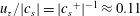 $u_{\unicode[STIX]{x1D70F}}/|c_{s}|=|{c_{s}}^{+}|^{-1}\approx 0.11$
, since
$u_{\unicode[STIX]{x1D70F}}/|c_{s}|=|{c_{s}}^{+}|^{-1}\approx 0.11$
, since
 $\unicode[STIX]{x1D70C}_{r}=1$
and
$\unicode[STIX]{x1D70C}_{r}=1$
and
 $Re_{\unicode[STIX]{x1D70F}}=720$
corresponds to
$Re_{\unicode[STIX]{x1D70F}}=720$
corresponds to
 $u_{\unicode[STIX]{x1D70F}}/U_{b}=0.053$
. The resulting instability region is marked with a white transparent area in figure 6.
$u_{\unicode[STIX]{x1D70F}}/U_{b}=0.053$
. The resulting instability region is marked with a white transparent area in figure 6.
The computed coating deformation is also not very reliable in a second region that is denoted as the ‘interaction region’: the significant coating deformation will influence the flow, which implies that the one-way coupling approach (as employed in this study) cannot be used reliably anymore. This region is differentiated by the requirement that at least one of the quantities
 $\{\unicode[STIX]{x1D709}_{c,rms}^{+},\unicode[STIX]{x1D701}_{c,rms}^{+},u_{c,rms}^{+},w_{c,rms}^{+}\}\gtrsim 1$
, as indicated with a black transparent area in figure 6. Note that this interaction region corresponds quite well to the area where resonances can be expected in the coating response. Figure 3 shows that resonances only occur when
$\{\unicode[STIX]{x1D709}_{c,rms}^{+},\unicode[STIX]{x1D701}_{c,rms}^{+},u_{c,rms}^{+},w_{c,rms}^{+}\}\gtrsim 1$
, as indicated with a black transparent area in figure 6. Note that this interaction region corresponds quite well to the area where resonances can be expected in the coating response. Figure 3 shows that resonances only occur when
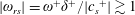 $|\unicode[STIX]{x1D714}_{rs}|=\unicode[STIX]{x1D714}^{+}\unicode[STIX]{x1D6FF}^{+}/|{c_{s}}^{+}|\gtrsim 1$
and
$|\unicode[STIX]{x1D714}_{rs}|=\unicode[STIX]{x1D714}^{+}\unicode[STIX]{x1D6FF}^{+}/|{c_{s}}^{+}|\gtrsim 1$
and
 $|c_{rs}|=(c/U_{b})\times (U_{b}/|c_{s}|)\gtrsim 1$
. The stress spectra of figure 5 indicate that the dominant frequencies are in the range
$|c_{rs}|=(c/U_{b})\times (U_{b}/|c_{s}|)\gtrsim 1$
. The stress spectra of figure 5 indicate that the dominant frequencies are in the range
 $\unicode[STIX]{x1D714}^{+}\lesssim 1$
, while the maximum convection velocity is typically smaller than the bulk velocity (
$\unicode[STIX]{x1D714}^{+}\lesssim 1$
, while the maximum convection velocity is typically smaller than the bulk velocity (
 $c/U_{b}\lesssim 1$
), such that the resonances will appear for sufficiently thick and soft coatings with
$c/U_{b}\lesssim 1$
), such that the resonances will appear for sufficiently thick and soft coatings with
 $\unicode[STIX]{x1D6FF}^{+}/|{c_{s}}^{+}|\gtrsim 1$
and
$\unicode[STIX]{x1D6FF}^{+}/|{c_{s}}^{+}|\gtrsim 1$
and
 $U_{b}/|c_{s}|\gtrsim 1$
. That part of the contour plots indeed shows anomalous behaviour, which is for instance apparent from the changed spacing and the wiggling of the contour lines.
$U_{b}/|c_{s}|\gtrsim 1$
. That part of the contour plots indeed shows anomalous behaviour, which is for instance apparent from the changed spacing and the wiggling of the contour lines.
Finally, the model results cannot be trusted in a third region which is called the ‘nonlinear region’, since it is characterized by nonlinear material behaviour that is not well represented by the linear coating model used in this study. This region, which is quantified with the criterion
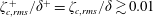 $\unicode[STIX]{x1D701}_{c,rms}^{+}/\unicode[STIX]{x1D6FF}^{+}=\unicode[STIX]{x1D701}_{c,rms}/\unicode[STIX]{x1D6FF}\gtrsim 0.01$
, is not sketched in figure 6 because it completely overlaps with the instability region and the interaction region.
$\unicode[STIX]{x1D701}_{c,rms}^{+}/\unicode[STIX]{x1D6FF}^{+}=\unicode[STIX]{x1D701}_{c,rms}/\unicode[STIX]{x1D6FF}\gtrsim 0.01$
, is not sketched in figure 6 because it completely overlaps with the instability region and the interaction region.
The coating softness has a pronounced influence on the deformation outside these three unreliable regions: figure 6 shows that the displacements and velocities are approximately proportional to
 $1/|{c_{s}}^{+}|^{2}\propto 1/|G|$
, the inverse of the shear modulus. This is in line with the observation that the displacement for relatively stiff coatings scales with
$1/|{c_{s}}^{+}|^{2}\propto 1/|G|$
, the inverse of the shear modulus. This is in line with the observation that the displacement for relatively stiff coatings scales with
 $\unicode[STIX]{x1D70C}_{r}|c_{rs}|^{2}$
(cf. (3.8), (3.10) and figure 4). Using that the convection velocity is proportional to the bulk velocity (
$\unicode[STIX]{x1D70C}_{r}|c_{rs}|^{2}$
(cf. (3.8), (3.10) and figure 4). Using that the convection velocity is proportional to the bulk velocity (
 $c\propto U_{b}$
), this dimensionless number can also be interpreted as the ratio of a fluid stress and a coating modulus:
$c\propto U_{b}$
), this dimensionless number can also be interpreted as the ratio of a fluid stress and a coating modulus:
 $$\begin{eqnarray}\unicode[STIX]{x1D70C}_{r}|c_{rs}|^{2}=\frac{\unicode[STIX]{x1D70C}_{f}}{\unicode[STIX]{x1D70C}_{s}}\frac{c^{2}}{|c_{s}|^{2}}\propto \frac{\unicode[STIX]{x1D70C}_{f}}{\unicode[STIX]{x1D70C}_{s}}\frac{U_{b}^{2}}{|c_{s}|^{2}}=\frac{\unicode[STIX]{x1D70C}_{f}U_{b}^{2}}{|G|}.\end{eqnarray}$$
It thus follows that the surface displacements and velocities are linearly proportional to
 $\unicode[STIX]{x1D70C}_{f}U_{b}^{2}/|G|$
, in agreement with Rosti & Brandt (Reference Rosti and Brandt2017).
$\unicode[STIX]{x1D70C}_{f}U_{b}^{2}/|G|$
, in agreement with Rosti & Brandt (Reference Rosti and Brandt2017).
The influence of the coating thickness reveals the long-wave and short-wave behaviour discussed in § 3.2. This is more clearly demonstrated in figure 7(a), which shows the r.m.s. surface displacements as a function of coating thickness
 $\unicode[STIX]{x1D6FF}^{+}$
for a given coating softness
$\unicode[STIX]{x1D6FF}^{+}$
for a given coating softness
 $|c_{s}^{+}|^{-1}$
, together with the results in the long-wave, low-frequency and short-wave limits. For very thin coatings, the displacements increase proportional to
$|c_{s}^{+}|^{-1}$
, together with the results in the long-wave, low-frequency and short-wave limits. For very thin coatings, the displacements increase proportional to
 $\unicode[STIX]{x1D6FF}^{+}$
(cf. (4.12)), which is characteristic of the long-wave response. For very thick coatings, the displacements become independent of the coating thickness
$\unicode[STIX]{x1D6FF}^{+}$
(cf. (4.12)), which is characteristic of the long-wave response. For very thick coatings, the displacements become independent of the coating thickness
 $\unicode[STIX]{x1D6FF}^{+}$
, which identifies the short-wave limit. Section 5.3 derives criteria to check whether the coating response is in the long-wave limit, the short-wave limit or in between.
$\unicode[STIX]{x1D6FF}^{+}$
, which identifies the short-wave limit. Section 5.3 derives criteria to check whether the coating response is in the long-wave limit, the short-wave limit or in between.

Figure 7. Root-mean-square surface displacements and velocities as functions of coating thickness (
 $\unicode[STIX]{x1D6FF}^{+}$
) for
$\unicode[STIX]{x1D6FF}^{+}$
) for
 $Re_{\unicode[STIX]{x1D70F}}=720$
,
$Re_{\unicode[STIX]{x1D70F}}=720$
,
 $\unicode[STIX]{x1D70C}_{r}=1$
,
$\unicode[STIX]{x1D70C}_{r}=1$
,
 $|{c_{s}}^{+}|^{-1}=0.02$
,
$|{c_{s}}^{+}|^{-1}=0.02$
,
 $\unicode[STIX]{x1D719}_{G}=10^{\circ }$
,
$\unicode[STIX]{x1D719}_{G}=10^{\circ }$
,
 $\unicode[STIX]{x1D708}_{pr}=0.45$
. (a) Surface displacements, including the results in the long-wave, low-frequency (lw) and short-wave (sw) limits. (b) Surface displacements and velocities.
$\unicode[STIX]{x1D708}_{pr}=0.45$
. (a) Surface displacements, including the results in the long-wave, low-frequency (lw) and short-wave (sw) limits. (b) Surface displacements and velocities.
The relative importance of the horizontal and vertical displacements and velocities can be clarified with figure 7(b). The trends in this figure are typical of almost any value of
 $|{c_{s}}^{+}|^{-1}$
. In particular, the horizontal and vertical displacements generally have a comparable magnitude. In the long-wave limit, the horizontal displacements can be larger than the vertical displacements, especially for materials that are close to incompressible. In the short-wave limit, the vertical displacement is larger (
$|{c_{s}}^{+}|^{-1}$
. In particular, the horizontal and vertical displacements generally have a comparable magnitude. In the long-wave limit, the horizontal displacements can be larger than the vertical displacements, especially for materials that are close to incompressible. In the short-wave limit, the vertical displacement is larger (
 $\unicode[STIX]{x1D701}_{c,rms}^{+}=0.20$
 ${>}$
${>}$
 $\unicode[STIX]{x1D709}_{c,rms}^{+}=0.097$
), although the horizontal displacement still has a comparable magnitude. Similarly, the horizontal and vertical velocities are always comparable in magnitude, although the vertical component is clearly larger than the horizontal component in the short-wave limit (
$\unicode[STIX]{x1D709}_{c,rms}^{+}=0.097$
), although the horizontal displacement still has a comparable magnitude. Similarly, the horizontal and vertical velocities are always comparable in magnitude, although the vertical component is clearly larger than the horizontal component in the short-wave limit (
 $u_{c,rms}^{+}=1.2\times 10^{-3}$
versus
$u_{c,rms}^{+}=1.2\times 10^{-3}$
versus
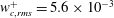 $w_{c,rms}^{+}=5.6\times 10^{-3}$
).
$w_{c,rms}^{+}=5.6\times 10^{-3}$
).
In comparing the displacements and velocities (figure 7(b)), two typical features can be noticed. First, the short-wave limit starts at a lower thickness for the velocities as compared to the displacements. Since the relations between the interface velocity and displacement for a certain mode
 $m$
are given by
$m$
are given by
 $u_{c,m}^{+}=\text{i}\unicode[STIX]{x1D714}_{m}^{+}\unicode[STIX]{x1D709}_{c,m}^{+}$
and
$u_{c,m}^{+}=\text{i}\unicode[STIX]{x1D714}_{m}^{+}\unicode[STIX]{x1D709}_{c,m}^{+}$
and
 $w_{c,m}^{+}=\text{i}\unicode[STIX]{x1D714}_{m}^{+}\unicode[STIX]{x1D701}_{c,m}^{+}$
, the higher frequencies are more prominent for the velocity, while the high frequencies are also the first to enter the short-wave regime. As a second observation, the interface velocity is smaller than the interface displacement when both are normalized in viscous units, which is typical for most parameters, especially in the short-wave limit. In that limit, the largest response comes from the longest wave with the lowest frequency (
$w_{c,m}^{+}=\text{i}\unicode[STIX]{x1D714}_{m}^{+}\unicode[STIX]{x1D701}_{c,m}^{+}$
, the higher frequencies are more prominent for the velocity, while the high frequencies are also the first to enter the short-wave regime. As a second observation, the interface velocity is smaller than the interface displacement when both are normalized in viscous units, which is typical for most parameters, especially in the short-wave limit. In that limit, the largest response comes from the longest wave with the lowest frequency (
 $\unicode[STIX]{x1D714}^{+}\ll 1$
), such that the relations
$\unicode[STIX]{x1D714}^{+}\ll 1$
), such that the relations
 $u_{c,m}^{+}=\text{i}\unicode[STIX]{x1D714}_{m}^{+}\unicode[STIX]{x1D709}_{c,m}^{+}$
and
$u_{c,m}^{+}=\text{i}\unicode[STIX]{x1D714}_{m}^{+}\unicode[STIX]{x1D709}_{c,m}^{+}$
and
 $w_{c,m}^{+}=\text{i}\unicode[STIX]{x1D714}_{m}^{+}\unicode[STIX]{x1D701}_{c,m}^{+}$
explain why
$w_{c,m}^{+}=\text{i}\unicode[STIX]{x1D714}_{m}^{+}\unicode[STIX]{x1D701}_{c,m}^{+}$
explain why
 $u_{c,rms}^{+}\ll \unicode[STIX]{x1D709}_{c,rms}^{+}$
and
$u_{c,rms}^{+}\ll \unicode[STIX]{x1D709}_{c,rms}^{+}$
and
 $w_{c,rms}^{+}\ll \unicode[STIX]{x1D701}_{c,rms}^{+}$
.
$w_{c,rms}^{+}\ll \unicode[STIX]{x1D701}_{c,rms}^{+}$
.

Figure 8. Point spectra of the surface displacements (a,c,e,g, logarithmic axes) and the surface velocities (b,d,f,h, linear axes) as functions of the angular frequency in viscous units for four parameter sets (see title inside panels, corresponding to the four dots in figure 6). The other parameters are
 $Re_{\unicode[STIX]{x1D70F}}=720$
,
$Re_{\unicode[STIX]{x1D70F}}=720$
,
 $\unicode[STIX]{x1D70C}_{r}=1$
,
$\unicode[STIX]{x1D70C}_{r}=1$
,
 $\unicode[STIX]{x1D719}_{G}=10^{\circ }$
,
$\unicode[STIX]{x1D719}_{G}=10^{\circ }$
,
 $\unicode[STIX]{x1D708}_{pr}=0.45$
. The square symbols on the top axes of the panels indicate the frequencies for which figure 9 shows a displacement vector field. The long-wave (lw) and short-wave (sw) results are included in the top and bottom panels, respectively.
$\unicode[STIX]{x1D708}_{pr}=0.45$
. The square symbols on the top axes of the panels indicate the frequencies for which figure 9 shows a displacement vector field. The long-wave (lw) and short-wave (sw) results are included in the top and bottom panels, respectively.
The type of coating response can be clarified with point spectra of the interface displacements and velocities, see figure 8. The displacement spectra (left, logarithmic axes) and velocity spectra (right, linear axes) are displayed for four different coatings, corresponding to the four dots in the contour plots of figure 6. For increasing coating thickness, the associated values of
 $\unicode[STIX]{x1D701}_{c,rms}^{+}$
are
$\unicode[STIX]{x1D701}_{c,rms}^{+}$
are
 $5.5\times 10^{-4}$
,
$5.5\times 10^{-4}$
,
 $6.9\times 10^{-2}$
,
$6.9\times 10^{-2}$
,
 $0.99$
and
$0.99$
and
 $4.1\times 10^{-4}$
.
$4.1\times 10^{-4}$
.
The first coating is very thin, which yields a characteristic long-wave response. The displacement spectra are the same as the stress spectra (figure 5), except for a mode-independent factor. The r.m.s. displacement is very well predicted by (4.12), which yields
 $\unicode[STIX]{x1D701}_{c,rms}^{+}=5.5\times 10^{-4}$
for
$\unicode[STIX]{x1D701}_{c,rms}^{+}=5.5\times 10^{-4}$
for
 $|c_{p}/c_{s}|=3.3$
. The velocity spectra are the displacement spectra multiplied with
$|c_{p}/c_{s}|=3.3$
. The velocity spectra are the displacement spectra multiplied with
 $(\unicode[STIX]{x1D714}^{+})^{2}$
, so the higher frequencies become more important.
$(\unicode[STIX]{x1D714}^{+})^{2}$
, so the higher frequencies become more important.
The second coating has the same softness as the first one, but it is thicker by a factor 80. A resonance starts to appear at the higher frequencies, close to
 $\unicode[STIX]{x1D714}^{+}=2$
,
$\unicode[STIX]{x1D714}^{+}=2$
,
 $|\unicode[STIX]{x1D714}_{rs}|=3.5$
,
$|\unicode[STIX]{x1D714}_{rs}|=3.5$
,
 $|c_{rs}|=1.1$
and
$|c_{rs}|=1.1$
and
 $\unicode[STIX]{x1D6FF}_{r\unicode[STIX]{x1D706}}=0.51$
. Note that Kim & Choi (Reference Kim and Choi2014) also report the appearance of a resonance in the frequency spectra of wall displacement and wall velocity. The resonance makes the long-wave expressions for the surface displacements inaccurate: equation (4.12) returns
$\unicode[STIX]{x1D6FF}_{r\unicode[STIX]{x1D706}}=0.51$
. Note that Kim & Choi (Reference Kim and Choi2014) also report the appearance of a resonance in the frequency spectra of wall displacement and wall velocity. The resonance makes the long-wave expressions for the surface displacements inaccurate: equation (4.12) returns
 $\unicode[STIX]{x1D701}_{c,rms}^{+}=4.4\times 10^{-2}$
, whereas the actual value is
$\unicode[STIX]{x1D701}_{c,rms}^{+}=4.4\times 10^{-2}$
, whereas the actual value is
 $\unicode[STIX]{x1D701}_{c,rms}^{+}=6.9\times 10^{-2}$
. The third coating has again the same softness, but it is approximately 6 times thicker than the second coating. The resonance now appears at lower frequencies, around
$\unicode[STIX]{x1D701}_{c,rms}^{+}=6.9\times 10^{-2}$
. The third coating has again the same softness, but it is approximately 6 times thicker than the second coating. The resonance now appears at lower frequencies, around
 $\unicode[STIX]{x1D714}^{+}=0.3$
, which corresponds with
$\unicode[STIX]{x1D714}^{+}=0.3$
, which corresponds with
 $|\unicode[STIX]{x1D714}_{rs}|=3.3$
,
$|\unicode[STIX]{x1D714}_{rs}|=3.3$
,
 $|c_{rs}|=1.1$
,
$|c_{rs}|=1.1$
,
 $\unicode[STIX]{x1D6FF}_{r\unicode[STIX]{x1D706}}=0.48$
. The long-wave prediction of
$\unicode[STIX]{x1D6FF}_{r\unicode[STIX]{x1D706}}=0.48$
. The long-wave prediction of
 $\unicode[STIX]{x1D701}_{c,rms}^{+}=0.28$
is again inaccurate compared to
$\unicode[STIX]{x1D701}_{c,rms}^{+}=0.28$
is again inaccurate compared to
 $\unicode[STIX]{x1D701}_{c,rms}^{+}=0.99$
.
$\unicode[STIX]{x1D701}_{c,rms}^{+}=0.99$
.
The fourth coating is very thick and very stiff, which yields a response that is characteristic for the short-wave limit. The displacements are proportional to the wavelength, so the largest wavelengths (corresponding to the lowest frequencies) dominate the spectra. The spectra follow the short-wave predictions very well, except for a small difference at the first frequency, corresponding to
 $\unicode[STIX]{x1D6FF}_{r\unicode[STIX]{x1D706}}=0.35$
, which is just on the border of the short-wave region (cf. figure 2).
$\unicode[STIX]{x1D6FF}_{r\unicode[STIX]{x1D706}}=0.35$
, which is just on the border of the short-wave region (cf. figure 2).
Figure 9 shows displacement vector fields for the four coatings just considered. The vector fields belong to the parameters that are indicated with a square in figures 2, 3(b) and 8. The selected frequencies belong to modes which make a large contribution to
 $w_{c,rms}^{+}$
(see figure 8). The first vector field corresponds to a low frequency and a long wavelength, as can be judged from the values of
$w_{c,rms}^{+}$
(see figure 8). The first vector field corresponds to a low frequency and a long wavelength, as can be judged from the values of
 $|\unicode[STIX]{x1D714}_{rs}|$
and
$|\unicode[STIX]{x1D714}_{rs}|$
and
 $\unicode[STIX]{x1D6FF}_{r\unicode[STIX]{x1D706}}$
in the figure title. The horizontal and vertical displacements are decoupled, although the ratio between both displacements stays the same due to the assumption of zero phase difference between the tangential and normal stresses.
$\unicode[STIX]{x1D6FF}_{r\unicode[STIX]{x1D706}}$
in the figure title. The horizontal and vertical displacements are decoupled, although the ratio between both displacements stays the same due to the assumption of zero phase difference between the tangential and normal stresses.
The vector fields for the second and third coating belong to modes close to resonance, which is not only evident from figure 8, but also from figure 3(b). The vector fields resemble vortices that are separated by half a wavelength. The parameters for the second coating are such that the horizontal surface displacement is close to zero, whereas the vertical displacement is significant.
The fourth vector field is characteristic for the short-wave response: the coating is much thicker than the wavelength, namely a factor 14 for this specific case. Note that only the top part of the coating is shown, i.e.
 $1.5\unicode[STIX]{x1D706}$
of the
$1.5\unicode[STIX]{x1D706}$
of the
 $14\unicode[STIX]{x1D706}$
in total. The deformation wave, which is only present near the surface, has a characteristic penetration depth of the order of one wavelength.
$14\unicode[STIX]{x1D706}$
in total. The deformation wave, which is only present near the surface, has a characteristic penetration depth of the order of one wavelength.
4.4.3 Viscoelasticity
Figure 10 displays how the surface displacement depends on the viscoelastic properties of the coating, the loss angle
 $\unicode[STIX]{x1D719}_{G}$
in particular. The four panels correspond to the four coatings that have been introduced above. The streamwise displacement of the first coating is not affected by
$\unicode[STIX]{x1D719}_{G}$
in particular. The four panels correspond to the four coatings that have been introduced above. The streamwise displacement of the first coating is not affected by
 $\unicode[STIX]{x1D719}_{G}$
, since
$\unicode[STIX]{x1D719}_{G}$
, since
 $\unicode[STIX]{x1D709}_{c,rms}^{+}$
in the long-wave limit only depends on the modulus magnitude
$\unicode[STIX]{x1D709}_{c,rms}^{+}$
in the long-wave limit only depends on the modulus magnitude
 $|G|$
, cf. (4.12). The vertical displacement is slightly affected by
$|G|$
, cf. (4.12). The vertical displacement is slightly affected by
 $\unicode[STIX]{x1D719}_{G}$
, as has been explained in the context of figure 4.
$\unicode[STIX]{x1D719}_{G}$
, as has been explained in the context of figure 4.

Figure 9. Displacement vector fields for four different sets of angular frequency (
 $\unicode[STIX]{x1D714}^{+}$
), coating thickness (
$\unicode[STIX]{x1D714}^{+}$
), coating thickness (
 $\unicode[STIX]{x1D6FF}^{+}$
) and coating softness (
$\unicode[STIX]{x1D6FF}^{+}$
) and coating softness (
 $|{c_{s}}^{+}|^{-1}$
) as given in the titles. The other parameters are
$|{c_{s}}^{+}|^{-1}$
) as given in the titles. The other parameters are
 $Re_{\unicode[STIX]{x1D70F}}=720$
,
$Re_{\unicode[STIX]{x1D70F}}=720$
,
 $\unicode[STIX]{x1D70C}_{r}=1$
,
$\unicode[STIX]{x1D70C}_{r}=1$
,
 $\unicode[STIX]{x1D719}_{G}=10^{\circ }$
,
$\unicode[STIX]{x1D719}_{G}=10^{\circ }$
,
 $\unicode[STIX]{x1D708}_{pr}=0.45$
. The coating thickness and softness correspond to the dots in the contour plots of figure 6. The frequencies are indicated with black squares in figure 8, whereas black squares in figures 2 and 3 provide the corresponding dimensionless parameters. The vertical axis is stretched (a) or compressed (b,c,d) for clarity and compactness. Panels (a–c) show the full coating thickness, whereas panel (d) contains only the top part of the coating (namely 1.5
$\unicode[STIX]{x1D708}_{pr}=0.45$
. The coating thickness and softness correspond to the dots in the contour plots of figure 6. The frequencies are indicated with black squares in figure 8, whereas black squares in figures 2 and 3 provide the corresponding dimensionless parameters. The vertical axis is stretched (a) or compressed (b,c,d) for clarity and compactness. Panels (a–c) show the full coating thickness, whereas panel (d) contains only the top part of the coating (namely 1.5
 $\unicode[STIX]{x1D706}$
, while the coating is 14
$\unicode[STIX]{x1D706}$
, while the coating is 14
 $\unicode[STIX]{x1D706}$
thick).
$\unicode[STIX]{x1D706}$
thick).

Figure 10. Horizontal and vertical surface displacement as functions of the loss angle
 $\unicode[STIX]{x1D719}_{G}$
for four parameter sets (see title, corresponding to the four dots in figure 6). The other parameters are
$\unicode[STIX]{x1D719}_{G}$
for four parameter sets (see title, corresponding to the four dots in figure 6). The other parameters are
 $Re_{\unicode[STIX]{x1D70F}}=720$
,
$Re_{\unicode[STIX]{x1D70F}}=720$
,
 $\unicode[STIX]{x1D70C}_{r}=1$
,
$\unicode[STIX]{x1D70C}_{r}=1$
,
 $\unicode[STIX]{x1D708}_{pr}=0.45$
. The long-wave (lw) and short-wave (sw) results are included in panels (a) and (d), respectively.
$\unicode[STIX]{x1D708}_{pr}=0.45$
. The long-wave (lw) and short-wave (sw) results are included in panels (a) and (d), respectively.
The deformation of the second and third coatings is quite sensitive to the loss angle when it is close to zero, which is due to the presence of resonances in the coating response (cf. figure 8). The displacements are very large for
 $\unicode[STIX]{x1D719}_{G}=0^{\circ }$
, which is attributed to the very strong resonances for an elastic coating (cf. figure 3(a); Kulik (Reference Kulik2012), Benschop & Breugem (Reference Benschop and Breugem2017)). The resonances are less pronounced for a viscoelastic solid (cf. figure 3), such that the surface displacements do not vary much for
$\unicode[STIX]{x1D719}_{G}=0^{\circ }$
, which is attributed to the very strong resonances for an elastic coating (cf. figure 3(a); Kulik (Reference Kulik2012), Benschop & Breugem (Reference Benschop and Breugem2017)). The resonances are less pronounced for a viscoelastic solid (cf. figure 3), such that the surface displacements do not vary much for
 $\unicode[STIX]{x1D719}_{G}\gtrsim 10^{\circ }$
.
$\unicode[STIX]{x1D719}_{G}\gtrsim 10^{\circ }$
.
The fourth coating is close to the short-wave limit, and the influence of the loss angle is small, in agreement with figure 4. Figure 10(d) shows that the short-wave predictions are slightly different from the actual values for the reason that the first frequency (which dominates the response) is just on the border of the short-wave region, as has been remarked in the context of figure 8. Overall, the surface displacements are relatively insensitive to changes in the loss angle as long as resonances in the coating response are absent.
4.4.4 Compressibility
Figure 11 displays how the surface displacement depends on the compressibility of the coating, the real part of Poisson’s ratio
 $\unicode[STIX]{x1D708}_{pr}$
in particular. The four panels correspond again to the four coatings that have been introduced above. The figures also show the deformations that result in the absence of shear stress, as will be discussed in the next subsection. The streamwise displacement of the first coating is not affected by the Poisson’s ratio, which is a consequence of the fact that
$\unicode[STIX]{x1D708}_{pr}$
in particular. The four panels correspond again to the four coatings that have been introduced above. The figures also show the deformations that result in the absence of shear stress, as will be discussed in the next subsection. The streamwise displacement of the first coating is not affected by the Poisson’s ratio, which is a consequence of the fact that
 $\unicode[STIX]{x1D709}_{c,rms}^{+}$
in the long-wave limit only depends on the shear modulus
$\unicode[STIX]{x1D709}_{c,rms}^{+}$
in the long-wave limit only depends on the shear modulus
 $G$
, independent of
$G$
, independent of
 $\unicode[STIX]{x1D708}_{pr}$
(cf. (4.12)). In contrast, the Poisson’s ratio has a significant influence on the vertical displacement: when
$\unicode[STIX]{x1D708}_{pr}$
(cf. (4.12)). In contrast, the Poisson’s ratio has a significant influence on the vertical displacement: when
 $\unicode[STIX]{x1D708}_{pr}\rightarrow 0.5$
, the compressional-wave modulus
$\unicode[STIX]{x1D708}_{pr}\rightarrow 0.5$
, the compressional-wave modulus
 $|\unicode[STIX]{x1D6F1}|\rightarrow \infty$
, such that the vertical displacement approaches zero (cf. (4.12), figure 4). The influence of the Poisson’s ratio is small for the other coatings: there is a slight change of
$|\unicode[STIX]{x1D6F1}|\rightarrow \infty$
, such that the vertical displacement approaches zero (cf. (4.12), figure 4). The influence of the Poisson’s ratio is small for the other coatings: there is a slight change of
 $\unicode[STIX]{x1D709}_{c,rms}^{+}$
, and
$\unicode[STIX]{x1D709}_{c,rms}^{+}$
, and
 $\unicode[STIX]{x1D701}_{c,rms}^{+}$
typically decreases with increasing
$\unicode[STIX]{x1D701}_{c,rms}^{+}$
typically decreases with increasing
 $\unicode[STIX]{x1D708}_{pr}$
, while it does not approach zero.
$\unicode[STIX]{x1D708}_{pr}$
, while it does not approach zero.

Figure 11. Horizontal and vertical surface displacement as functions of the real part of Poisson’s ratio
 $\unicode[STIX]{x1D708}_{pr}$
for four parameter sets (see title, corresponding to the four dots in figure 6). The other parameters are
$\unicode[STIX]{x1D708}_{pr}$
for four parameter sets (see title, corresponding to the four dots in figure 6). The other parameters are
 $Re_{\unicode[STIX]{x1D70F}}=720$
,
$Re_{\unicode[STIX]{x1D70F}}=720$
,
 $\unicode[STIX]{x1D70C}_{r}=1$
,
$\unicode[STIX]{x1D70C}_{r}=1$
,
 $\unicode[STIX]{x1D719}_{G}=10^{\circ }$
.
$\unicode[STIX]{x1D719}_{G}=10^{\circ }$
.
4.4.5 Influence of shear stress
To determine whether the shear stress has an important contribution to the surface deformation, figure 11 also shows the displacements that result in the absence of shear stress (
 $\unicode[STIX]{x1D70E}_{tc}=0$
). The influence of shear on the vertical displacement is marginal for all cases: the difference between the curves with and without shear stress is barely visible. The vertical displacement is thus predominantly determined by the normal stress, in agreement with similar observations by other researchers (Kulik Reference Kulik2012; Zhang et al.
Reference Zhang, Wang, Blake and Katz2017).
$\unicode[STIX]{x1D70E}_{tc}=0$
). The influence of shear on the vertical displacement is marginal for all cases: the difference between the curves with and without shear stress is barely visible. The vertical displacement is thus predominantly determined by the normal stress, in agreement with similar observations by other researchers (Kulik Reference Kulik2012; Zhang et al.
Reference Zhang, Wang, Blake and Katz2017).
The influence of the shear stress on the horizontal displacement is, however, more pronounced:
 $\unicode[STIX]{x1D709}_{c,rms}^{+}$
decreases in absence of shear for all cases. The reduction is most substantial in the long-wave limit, i.e. for very thin and stiff coatings: the horizontal deformation is then solely driven by the shear stress (cf. (4.12)), so
$\unicode[STIX]{x1D709}_{c,rms}^{+}$
decreases in absence of shear for all cases. The reduction is most substantial in the long-wave limit, i.e. for very thin and stiff coatings: the horizontal deformation is then solely driven by the shear stress (cf. (4.12)), so
 $\unicode[STIX]{x1D709}_{c,rms}^{+}=0$
when shear is absent. For the other three cases shown in figure 11, the removal of shear results in a decrease of the horizontal displacement by a factor of approximately 1.7, 1.4 and 4.8.
$\unicode[STIX]{x1D709}_{c,rms}^{+}=0$
when shear is absent. For the other three cases shown in figure 11, the removal of shear results in a decrease of the horizontal displacement by a factor of approximately 1.7, 1.4 and 4.8.

Figure 12. Influence of the phase angle of the stress waves on the root-mean-square value of the surface displacements. The displacements were calculated for 1000 sets of random angles for all the 995 shear and pressure waves. The results are shown as histograms with 20 bins for four parameter sets (see title, corresponding to the four dots in figure 6).
 $P$
represents the probability to find a displacement within a certain bin; the sum of all the bar heights equals 1. The markers on the bottom axes correspond to stresses for which all phases are zero (
$P$
represents the probability to find a displacement within a certain bin; the sum of all the bar heights equals 1. The markers on the bottom axes correspond to stresses for which all phases are zero (
 $\unicode[STIX]{x1D719}_{tc,m}=0=\unicode[STIX]{x1D719}_{nc,m}$
for all
$\unicode[STIX]{x1D719}_{tc,m}=0=\unicode[STIX]{x1D719}_{nc,m}$
for all
 $m$
), as is assumed throughout the paper. The other parameters are
$m$
), as is assumed throughout the paper. The other parameters are
 $Re_{\unicode[STIX]{x1D70F}}=720$
,
$Re_{\unicode[STIX]{x1D70F}}=720$
,
 $\unicode[STIX]{x1D70C}_{r}=1$
,
$\unicode[STIX]{x1D70C}_{r}=1$
,
 $\unicode[STIX]{x1D719}_{G}=10^{\circ }$
,
$\unicode[STIX]{x1D719}_{G}=10^{\circ }$
,
 $\unicode[STIX]{x1D708}_{pr}=0.45$
.
$\unicode[STIX]{x1D708}_{pr}=0.45$
.
4.4.6 Phase angle of stress waves
The stresses of the individual waves not only have an amplitude, but also a phase (cf. § 4.2.2). It has been noted in the context of (4.6) that the influence of these phases on the deformation is small, which is quantified here for the four coatings that have been considered above. The surface displacements were calculated for 1000 sets of random angles for all the 995 shear and pressure modes, and the results are shown in figure 12 as histograms of
 $\unicode[STIX]{x1D709}_{c,rms}^{+}$
and
$\unicode[STIX]{x1D709}_{c,rms}^{+}$
and
 $\unicode[STIX]{x1D701}_{c,rms}^{+}$
for the four parameter sets. There is practically no difference for the first coating, as the r.m.s. of the displacements only depends on the r.m.s. of the surface stresses (4.12). There is some influence of the phase for the other coatings, especially for the very thick one, but the spreading is not huge since the order of magnitude of the surface displacements remains unchanged.
$\unicode[STIX]{x1D701}_{c,rms}^{+}$
for the four parameter sets. There is practically no difference for the first coating, as the r.m.s. of the displacements only depends on the r.m.s. of the surface stresses (4.12). There is some influence of the phase for the other coatings, especially for the very thick one, but the spreading is not huge since the order of magnitude of the surface displacements remains unchanged.
5 Coating deformation in turbulent boundary-layer flow
This section applies the presented model to turbulent boundary-layer flow in order to allow a comparison with recent experiments. The first subsection outlines the experiments, followed by a description of the analytical model in the second subsection, some additional remarks regarding the long-wave and short-wave coating response in the third subsection and a comparison with the experiments in the last subsection.
5.1 Experiments
The deformation of a compliant coating on a rigid wall underneath a turbulent boundary-layer flow was studied experimentally. Preliminary results were presented by Delfos et al. (Reference Delfos, Greidanus, Charruault and Westerweel2017) and Greidanus et al. (Reference Greidanus, Delfos and Westerweel2017), whose work was continued to allow a comparison with the model proposed in this paper. Three coatings were produced in-house, applied to a rigid plate and tested in a water tunnel. Three quantities were measured, namely the flow velocity with planar particle image velocimetry (PIV, Adrian & Westerweel (Reference Adrian and Westerweel2011)), the drag force on the plate with a force balance and the vertical coating displacement with high-speed background-oriented schlieren (BOS, Raffel Reference Raffel2015). Below, we provide a short description of the water tunnel, the flow, the drag force, the three coatings and the deformation measurements.
The water tunnel has an optically fully accessible test section that has a length of 2 m and an inlet with a cross-sectional area of
 $300\times 300~\text{mm}^{2}$
. The top wall of the test section can be replaced to mount the test plates with a surface area of
$300\times 300~\text{mm}^{2}$
. The top wall of the test section can be replaced to mount the test plates with a surface area of
 $1998\times 297~\text{mm}^{2}$
. The PIV and BOS measurements were performed at 1.7 m downstream of the test section’s entrance.
$1998\times 297~\text{mm}^{2}$
. The PIV and BOS measurements were performed at 1.7 m downstream of the test section’s entrance.
The flow properties are listed in table 1, e.g. the free-stream velocity
 $U_{\infty }$
was varied from about 0.9 to
$U_{\infty }$
was varied from about 0.9 to
 $5.4~\text{m}~\text{s}^{-1}$
. The velocity profiles, as measured by PIV, approximately satisfy
$5.4~\text{m}~\text{s}^{-1}$
. The velocity profiles, as measured by PIV, approximately satisfy
 $u/U_{\infty }=(z/\unicode[STIX]{x1D6FF}_{bl})^{1/8}$
, with streamwise velocity
$u/U_{\infty }=(z/\unicode[STIX]{x1D6FF}_{bl})^{1/8}$
, with streamwise velocity
 $u$
, the vertical distance to the surface
$u$
, the vertical distance to the surface
 $z$
, and the boundary-layer thickness
$z$
, and the boundary-layer thickness
 $\unicode[STIX]{x1D6FF}_{bl}$
(note the difference with the coating thickness
$\unicode[STIX]{x1D6FF}_{bl}$
(note the difference with the coating thickness
 $\unicode[STIX]{x1D6FF}$
). The momentum thickness
$\unicode[STIX]{x1D6FF}$
). The momentum thickness
 $\unicode[STIX]{x1D703}$
was computed by integration of the velocity profiles, and the boundary-layer thickness then followed from the relation
$\unicode[STIX]{x1D703}$
was computed by integration of the velocity profiles, and the boundary-layer thickness then followed from the relation
 $\unicode[STIX]{x1D6FF}_{bl}=(45/4)\unicode[STIX]{x1D703}$
for velocity profiles with a power
$\unicode[STIX]{x1D6FF}_{bl}=(45/4)\unicode[STIX]{x1D703}$
for velocity profiles with a power
 $1/8$
. The thus obtained boundary-layer thickness follows quite well the power law
$1/8$
. The thus obtained boundary-layer thickness follows quite well the power law
 $\unicode[STIX]{x1D6FF}_{bl}=0.057U_{\infty }^{-1/7}$
, which was henceforth used to compute the boundary-layer thickness for a given free-stream velocity. From now on, the superscript
$\unicode[STIX]{x1D6FF}_{bl}=0.057U_{\infty }^{-1/7}$
, which was henceforth used to compute the boundary-layer thickness for a given free-stream velocity. From now on, the superscript
 $^{o}$
is used to denote quantities that are normalized with outer units (
$^{o}$
is used to denote quantities that are normalized with outer units (
 $U_{\infty }$
and
$U_{\infty }$
and
 $\unicode[STIX]{x1D6FF}_{bl}$
):
$\unicode[STIX]{x1D6FF}_{bl}$
):
 $$\begin{eqnarray}\unicode[STIX]{x1D714}^{o}=\frac{\unicode[STIX]{x1D714}\unicode[STIX]{x1D6FF}_{bl}}{U_{\infty }},\quad k^{o}=k\unicode[STIX]{x1D6FF}_{bl},\quad c^{o}=\frac{c}{U_{\infty }}.\end{eqnarray}$$
Drag measurements were performed both on smooth rigid plates and on coated plates. The force balance measured the total drag on the whole test plate, from which the plate-averaged shear stress
 $\langle \unicode[STIX]{x1D70F}_{w}\rangle _{}$
was obtained. The local shear stress
$\langle \unicode[STIX]{x1D70F}_{w}\rangle _{}$
was obtained. The local shear stress
 $\unicode[STIX]{x1D70F}_{w}$
(at the location of the PIV and BOS measurements) was estimated from
$\unicode[STIX]{x1D70F}_{w}$
(at the location of the PIV and BOS measurements) was estimated from
 $\unicode[STIX]{x1D70F}_{w}=(6/7)\langle \unicode[STIX]{x1D70F}_{w}\rangle _{}$
(Greidanus et al.
Reference Greidanus, Delfos and Westerweel2017), and the local wall-friction velocity then followed from
$\unicode[STIX]{x1D70F}_{w}=(6/7)\langle \unicode[STIX]{x1D70F}_{w}\rangle _{}$
(Greidanus et al.
Reference Greidanus, Delfos and Westerweel2017), and the local wall-friction velocity then followed from
 $u_{\unicode[STIX]{x1D70F}}=\sqrt{\unicode[STIX]{x1D70F}_{w}/\unicode[STIX]{x1D70C}_{f}}$
. A fit to the thus obtained shear velocity yields the power law
$u_{\unicode[STIX]{x1D70F}}=\sqrt{\unicode[STIX]{x1D70F}_{w}/\unicode[STIX]{x1D70C}_{f}}$
. A fit to the thus obtained shear velocity yields the power law
 $u_{\unicode[STIX]{x1D70F}}=0.041U_{\infty }^{0.91}$
for the smooth rigid wall. Like in the analytical model, viscous scaling is based on the shear velocity of the smooth-wall flow. Next, three different Reynolds numbers can be defined:
$u_{\unicode[STIX]{x1D70F}}=0.041U_{\infty }^{0.91}$
for the smooth rigid wall. Like in the analytical model, viscous scaling is based on the shear velocity of the smooth-wall flow. Next, three different Reynolds numbers can be defined:
 $$\begin{eqnarray}Re_{\unicode[STIX]{x1D70F}}=\frac{\unicode[STIX]{x1D6FF}_{bl}u_{\unicode[STIX]{x1D70F}}}{\unicode[STIX]{x1D708}},\quad Re_{\unicode[STIX]{x1D6FF}}=\frac{\unicode[STIX]{x1D6FF}_{bl}U_{\infty }}{\unicode[STIX]{x1D708}},\quad R_{T}=\frac{\unicode[STIX]{x1D6FF}_{bl}/U_{\infty }}{\unicode[STIX]{x1D708}/u_{\unicode[STIX]{x1D70F}}^{2}}=\frac{Re_{\unicode[STIX]{x1D70F}}^{2}}{Re_{\unicode[STIX]{x1D6FF}}},\end{eqnarray}$$
where
 $R_{T}$
represents the ratio of the outer layer to inner layer time scale that appears later in the analytical model. Note that table 1 provides the range of the numerical values for the free-stream velocity, boundary-layer thickness, shear velocity and three Reynolds numbers.
$R_{T}$
represents the ratio of the outer layer to inner layer time scale that appears later in the analytical model. Note that table 1 provides the range of the numerical values for the free-stream velocity, boundary-layer thickness, shear velocity and three Reynolds numbers.
Table 1. Properties of the turbulent boundary-layer flow in the experiments.

The properties of the three coatings are given in table 2: all coatings have the same thickness of 5 mm and approximately the same mass density. In contrast, the moduli of the coatings are significantly different, with coating 1 being the softest and coating 3 the stiffest. The frequency-dependent shear modulus (
 $G=G_{1}+\text{i}G_{2}$
) of the three coatings was measured using a commercial rheometer (ARES-G2, TA Instruments) with a parallel plate geometry of 25 mm in diameter. Specifically, the storage modulus
$G=G_{1}+\text{i}G_{2}$
) of the three coatings was measured using a commercial rheometer (ARES-G2, TA Instruments) with a parallel plate geometry of 25 mm in diameter. Specifically, the storage modulus
 $G_{1}$
and the loss modulus
$G_{1}$
and the loss modulus
 $G_{2}$
were measured in a frequency range of
$G_{2}$
were measured in a frequency range of
 $\unicode[STIX]{x1D714}=0.1~\text{rad}~\text{s}^{-1}$
to
$\unicode[STIX]{x1D714}=0.1~\text{rad}~\text{s}^{-1}$
to
 $\unicode[STIX]{x1D714}=100~\text{rad}~\text{s}^{-1}$
at
$\unicode[STIX]{x1D714}=100~\text{rad}~\text{s}^{-1}$
at
 $20\,^{\circ }\text{C}$
and 0.5 % strain. The measurements were limited to
$20\,^{\circ }\text{C}$
and 0.5 % strain. The measurements were limited to
 $100~\text{rad}~\text{s}^{-1}$
, which is the maximum frequency that the rheometer could reach. In theory, modulus values at higher frequencies can be obtained with use of the time–temperature superposition (TTS) principle. In practice, however, measurements below room temperature resulted in vapour condensation on the measurement facility and the samples, such that the obtained values were considered unreliable. The table lists the values at
$100~\text{rad}~\text{s}^{-1}$
, which is the maximum frequency that the rheometer could reach. In theory, modulus values at higher frequencies can be obtained with use of the time–temperature superposition (TTS) principle. In practice, however, measurements below room temperature resulted in vapour condensation on the measurement facility and the samples, such that the obtained values were considered unreliable. The table lists the values at
 $100~\text{rad}~\text{s}^{-1}$
, as that turned out to be the frequency closest to the most dominant frequency in the coating response. There is one exception: the loss properties at
$100~\text{rad}~\text{s}^{-1}$
, as that turned out to be the frequency closest to the most dominant frequency in the coating response. There is one exception: the loss properties at
 $100~\text{rad}~\text{s}^{-1}$
for coating 1 are
$100~\text{rad}~\text{s}^{-1}$
for coating 1 are
 $G_{2}=0.20$
kPa and
$G_{2}=0.20$
kPa and
 $\unicode[STIX]{x1D719}_{G}=8.1^{\circ }$
, while the table provides somewhat larger values, as is motivated in the context of the displacement spectra in § 5.4. While the shear modulus of the three coatings is of the order of kPa, the bulk modulus is of the order of GPa, such that the coatings are practically incompressible:
$\unicode[STIX]{x1D719}_{G}=8.1^{\circ }$
, while the table provides somewhat larger values, as is motivated in the context of the displacement spectra in § 5.4. While the shear modulus of the three coatings is of the order of kPa, the bulk modulus is of the order of GPa, such that the coatings are practically incompressible:
 $\unicode[STIX]{x1D708}_{pr}\approx 0.5$
.
$\unicode[STIX]{x1D708}_{pr}\approx 0.5$
.
Small height variations of the optically transparent coating were measured with the background-oriented schlieren (BOS) method of Moisy, Rabaud & Salsac (Reference Moisy, Rabaud and Salsac2009), which they call a synthetic schlieren method. A high-speed camera was used for time-resolved measurements of the optical distortion of a random dot pattern, placed behind the coating, due to refraction of light at the deforming coating interface. The displacement field of the dots was determined from digital image correlation (DIC, Adrian & Westerweel Reference Adrian and Westerweel2011) between the deformed and the undeformed dot pattern. The dot displacements were related to the interface slope, and the vertical interface displacement was subsequently obtained from spatial integration. This method was applied at approximately 180
 $\times$
180 points within a field of view of size
$\times$
180 points within a field of view of size
 $100\times 100~\text{mm}^{2}$
. The measurement signals contain 2000 time samples with a measurement frequency
$100\times 100~\text{mm}^{2}$
. The measurement signals contain 2000 time samples with a measurement frequency
 $f$
, which was fixed at
$f$
, which was fixed at
 $f=1200$
Hz for coating 1. It was increased in linear proportion to the free-stream velocity for coatings 2 and 3, namely from
$f=1200$
Hz for coating 1. It was increased in linear proportion to the free-stream velocity for coatings 2 and 3, namely from
 $f=200$
Hz at
$f=200$
Hz at
 $U_{\infty }=0.87~\text{m}~\text{s}^{-1}$
to
$U_{\infty }=0.87~\text{m}~\text{s}^{-1}$
to
 $f=1240$
Hz at
$f=1240$
Hz at
 $U_{\infty }=5.39~\text{m}~\text{s}^{-1}$
.
$U_{\infty }=5.39~\text{m}~\text{s}^{-1}$
.
Table 2. Properties of the coatings employed in the experiments, together with the dimensionless numbers that the analytical model requires to predict the coating deformation.

The long-wave coating deformation could not be reliably measured. Specifically, long waves result in displacement fields that are almost spatially uniform, whereas plate vibrations also result in such uniform fields. As independent measurements of the plate position were not performed, the distinction between long-wave coating deformations and plate vibrations could not be made. Therefore, coating deformation waves with a wavelength larger than the length of the field of view (i.e.
 $\unicode[STIX]{x1D706}>\unicode[STIX]{x1D706}_{max}=100$
mm) could not be quantified reliably.
$\unicode[STIX]{x1D706}>\unicode[STIX]{x1D706}_{max}=100$
mm) could not be quantified reliably.
Since long waves could not be accurately measured, the same is true for low frequencies. Specifically, the minimum frequency that can be measured relates to the maximum wavelength according to
 $\unicode[STIX]{x1D714}_{min}=2\unicode[STIX]{x03C0}c/\unicode[STIX]{x1D706}_{max}$
or
$\unicode[STIX]{x1D714}_{min}=2\unicode[STIX]{x03C0}c/\unicode[STIX]{x1D706}_{max}$
or
 $\unicode[STIX]{x1D714}_{min}^{o}=2\unicode[STIX]{x03C0}c^{o}/\unicode[STIX]{x1D706}_{max}^{\circ }$
. Given that
$\unicode[STIX]{x1D714}_{min}^{o}=2\unicode[STIX]{x03C0}c^{o}/\unicode[STIX]{x1D706}_{max}^{\circ }$
. Given that
 $\unicode[STIX]{x1D706}_{max}^{\circ }=\unicode[STIX]{x1D706}_{max}/\unicode[STIX]{x1D6FF}_{bl}$
increases from 1.7 to 2.2, and assuming that
$\unicode[STIX]{x1D706}_{max}^{\circ }=\unicode[STIX]{x1D706}_{max}/\unicode[STIX]{x1D6FF}_{bl}$
increases from 1.7 to 2.2, and assuming that
 $c^{o}=c/U_{\infty }\approx 0.75$
(Delfos et al.
Reference Delfos, Greidanus, Charruault and Westerweel2017), it follows that
$c^{o}=c/U_{\infty }\approx 0.75$
(Delfos et al.
Reference Delfos, Greidanus, Charruault and Westerweel2017), it follows that
 $\unicode[STIX]{x1D714}_{min}^{o}$
varies between 2.8 and 2.1. The low-frequency response (
$\unicode[STIX]{x1D714}_{min}^{o}$
varies between 2.8 and 2.1. The low-frequency response (
 $\unicode[STIX]{x1D714}\lesssim \unicode[STIX]{x1D714}_{min}$
) is most likely attributable to non-advected features that could result from resonances or reflected waves associated with the finite length of the compliant wall (Zhang et al.
Reference Zhang, Wang, Blake and Katz2017). Indeed, the response below
$\unicode[STIX]{x1D714}\lesssim \unicode[STIX]{x1D714}_{min}$
) is most likely attributable to non-advected features that could result from resonances or reflected waves associated with the finite length of the compliant wall (Zhang et al.
Reference Zhang, Wang, Blake and Katz2017). Indeed, the response below
 $\unicode[STIX]{x1D714}_{min}^{o}$
partially results from pronounced tunnel vibrations at
$\unicode[STIX]{x1D714}_{min}^{o}$
partially results from pronounced tunnel vibrations at
 $f=5$
Hz (independent of flow velocity), which corresponds with a dimensionless frequency
$f=5$
Hz (independent of flow velocity), which corresponds with a dimensionless frequency
 $\unicode[STIX]{x1D714}^{o}$
that decreases from 2.1 to 0.26 when the flow velocity increases.
$\unicode[STIX]{x1D714}^{o}$
that decreases from 2.1 to 0.26 when the flow velocity increases.
The focus of the present study is on advected phenomena, as in the study by Zhang et al. (Reference Zhang, Wang, Blake and Katz2017). For that reason, the measured surface displacement was filtered to exclude frequencies below
 $\unicode[STIX]{x1D714}_{min}^{o}$
. First, the displacement point spectra were computed using fast Fourier transform (FFT): the time signal was written as
$\unicode[STIX]{x1D714}_{min}^{o}$
. First, the displacement point spectra were computed using fast Fourier transform (FFT): the time signal was written as
 $\unicode[STIX]{x1D701}(t)=\sum _{m}\unicode[STIX]{x1D701}_{m}\exp (\text{i}\unicode[STIX]{x1D714}_{m}t)$
, the amplitudes
$\unicode[STIX]{x1D701}(t)=\sum _{m}\unicode[STIX]{x1D701}_{m}\exp (\text{i}\unicode[STIX]{x1D714}_{m}t)$
, the amplitudes
 $\unicode[STIX]{x1D701}_{m}$
were obtained from the FFT and the point spectra followed from (C 6a
). Next, frequencies below
$\unicode[STIX]{x1D701}_{m}$
were obtained from the FFT and the point spectra followed from (C 6a
). Next, frequencies below
 $\unicode[STIX]{x1D714}_{min}^{o}$
were removed from the spectra. To smooth the quite spiky spectra, a filtered time signal was reconstructed from an inverse FFT, this time signal was cut in 40 pieces of 50 time samples each and a spectrum was computed for each piece using the FFT. Finally, the spectra were averaged over all pieces and all points within the field of view. For all coatings and flow velocities, the r.m.s. of the filtered data varied between 83 and 98 % of the r.m.s. for the unfiltered data.
$\unicode[STIX]{x1D714}_{min}^{o}$
were removed from the spectra. To smooth the quite spiky spectra, a filtered time signal was reconstructed from an inverse FFT, this time signal was cut in 40 pieces of 50 time samples each and a spectrum was computed for each piece using the FFT. Finally, the spectra were averaged over all pieces and all points within the field of view. For all coatings and flow velocities, the r.m.s. of the filtered data varied between 83 and 98 % of the r.m.s. for the unfiltered data.
5.2 Analytical model
The analytical model requires the turbulent stress spectra, the convection velocity and the frequency-dependent coating properties as input, as described below in more detail. Several models for the turbulent pressure spectra exist, as reviewed by Hwang et al. (Reference Hwang, Bonness and Hambric2009). According to their review, the model by Goody (Reference Goody2004) provides the best overall prediction of the spectra. It is given by:
 $$\begin{eqnarray}E_{\unicode[STIX]{x1D70E}_{nc}^{+}}^{^{o}}=\frac{E_{\unicode[STIX]{x1D70E}_{nc}}(\unicode[STIX]{x1D714})U_{\infty }}{\unicode[STIX]{x1D70F}_{w}^{2}\unicode[STIX]{x1D6FF}_{bl}}=\frac{C_{2}(\unicode[STIX]{x1D714}\unicode[STIX]{x1D6FF}_{bl}/U_{\infty })^{2}}{\left[(\unicode[STIX]{x1D714}\unicode[STIX]{x1D6FF}_{bl}/U_{\infty })^{0.75}+C_{1}\right]^{3.7}+\left[C_{3}(\unicode[STIX]{x1D714}\unicode[STIX]{x1D6FF}_{bl}/U_{\infty })\right]^{7}},\end{eqnarray}$$
with model parameters
 $C_{1}=0.5$
,
$C_{1}=0.5$
,
 $C_{2}=3.0$
and
$C_{2}=3.0$
and
 $C_{3}=1.1R_{T}^{-0.57}$
. The spectrum is defined as
$C_{3}=1.1R_{T}^{-0.57}$
. The spectrum is defined as
 $E_{\unicode[STIX]{x1D70E}_{nc}^{+}}^{^{o}}=E_{\unicode[STIX]{x1D70E}_{nc}^{+}}U_{\infty }/\unicode[STIX]{x1D6FF}_{bl}$
, which is the spectrum
$E_{\unicode[STIX]{x1D70E}_{nc}^{+}}^{^{o}}=E_{\unicode[STIX]{x1D70E}_{nc}^{+}}U_{\infty }/\unicode[STIX]{x1D6FF}_{bl}$
, which is the spectrum
 $E_{\unicode[STIX]{x1D70E}_{nc}^{+}}$
normalized in outer units, where
$E_{\unicode[STIX]{x1D70E}_{nc}^{+}}$
normalized in outer units, where
 $E_{\unicode[STIX]{x1D70E}_{nc}^{+}}=E_{\unicode[STIX]{x1D70E}_{nc}}/\unicode[STIX]{x1D70F}_{w}^{2}$
represents the spectrum of
$E_{\unicode[STIX]{x1D70E}_{nc}^{+}}=E_{\unicode[STIX]{x1D70E}_{nc}}/\unicode[STIX]{x1D70F}_{w}^{2}$
represents the spectrum of
 $\unicode[STIX]{x1D70E}_{nc}^{+}$
. Note that
$\unicode[STIX]{x1D70E}_{nc}^{+}$
. Note that
 $E_{\unicode[STIX]{x1D70E}_{nc}^{+}}^{^{o}}$
depends on
$E_{\unicode[STIX]{x1D70E}_{nc}^{+}}^{^{o}}$
depends on
 $\unicode[STIX]{x1D714}$
in the ratio
$\unicode[STIX]{x1D714}$
in the ratio
 $\unicode[STIX]{x1D714}\unicode[STIX]{x1D6FF}_{bl}/U_{\infty }=\unicode[STIX]{x1D714}^{o}$
, which is the frequency normalized with a characteristic frequency of the outer layer. The ratio of
$\unicode[STIX]{x1D714}\unicode[STIX]{x1D6FF}_{bl}/U_{\infty }=\unicode[STIX]{x1D714}^{o}$
, which is the frequency normalized with a characteristic frequency of the outer layer. The ratio of
 $C_{1}$
to
$C_{1}$
to
 $C_{3}$
determines the size of the overlap range, which depends on the ratio
$C_{3}$
determines the size of the overlap range, which depends on the ratio
 $R_{T}$
of the outer layer to inner layer time scale (cf. (5.2)).
$R_{T}$
of the outer layer to inner layer time scale (cf. (5.2)).
Figure 13(a) displays the Goody spectrum at four different Reynolds numbers that are typical for the experiments. The spectra collapse for low frequencies because outer scaling is used, while inner scaling will collapse the spectra at high frequencies. The extent of the overlap range increases with increasing Reynolds number. Hwang et al. (Reference Hwang, Bonness and Hambric2009) provide more information about the use of different scales to collapse the spectra in different frequency regions. The Goody spectrum at
 $Re_{\unicode[STIX]{x1D70F}}=720$
is very similar to the channel-flow spectrum of Hu et al. (Reference Hu, Morfey and Sandham2006) (figure 5), except that the latter does not include the very low frequencies for which the Goody spectrum exhibits a decay when
$Re_{\unicode[STIX]{x1D70F}}=720$
is very similar to the channel-flow spectrum of Hu et al. (Reference Hu, Morfey and Sandham2006) (figure 5), except that the latter does not include the very low frequencies for which the Goody spectrum exhibits a decay when
 $\unicode[STIX]{x1D714}\rightarrow 0$
.
$\unicode[STIX]{x1D714}\rightarrow 0$
.

Figure 13. Pressure spectrum (a) and convection velocity (b) as functions of frequency for four Reynolds numbers, using outer scaling. The pressure spectrum was obtained from the analytical relation provided by Goody (Reference Goody2004) for turbulent boundary-layer flow (5.3). The convection velocity was calculated from a model that Del Álamo & Jiménez (Reference Del Álamo and Jiménez2009) derived from DNS data of turbulent channel flow.
An important characteristic of the spectrum is its integral, which provides a measure of the root-mean-square (r.m.s.) of the fluctuations. Goody (Reference Goody2002) obtained a relation (their equation 8) that should describe the variation of the mean square pressure with
 $R_{T}$
for the Goody spectrum. His relation, however, does not yield the numerical values that were reported in table 3 from his paper, which explains why we propose a slightly different relation. The Goody spectrum was integrated numerically for a range of
$R_{T}$
for the Goody spectrum. His relation, however, does not yield the numerical values that were reported in table 3 from his paper, which explains why we propose a slightly different relation. The Goody spectrum was integrated numerically for a range of
 $R_{T}$
between
$R_{T}$
between
 $10$
and
$10$
and
 $10^{3}$
, using (C 6b
) for logarithmically distributed frequencies in the range
$10^{3}$
, using (C 6b
) for logarithmically distributed frequencies in the range
 $\unicode[STIX]{x1D714}^{o}=10^{-4}$
to
$\unicode[STIX]{x1D714}^{o}=10^{-4}$
to
 $\unicode[STIX]{x1D714}^{o}=10^{4}$
. The resulting r.m.s.-values were fitted to the following curve:
$\unicode[STIX]{x1D714}^{o}=10^{4}$
. The resulting r.m.s.-values were fitted to the following curve:
 $$\begin{eqnarray}\displaystyle (\unicode[STIX]{x1D70E}_{nc,rms}^{+})^{2}=0.0309+0.745(\ln (R_{T}))^{2},\end{eqnarray}$$
which is the same relation as in Goody (Reference Goody2002), except for the different coefficients. Given that
 $R_{T}$
in the experiments varied between 83 and 300 (table 1), the corresponding pressure r.m.s.
$R_{T}$
in the experiments varied between 83 and 300 (table 1), the corresponding pressure r.m.s.
 $\unicode[STIX]{x1D70E}_{nc,rms}^{+}$
ranges from 3.8 to 4.9.
$\unicode[STIX]{x1D70E}_{nc,rms}^{+}$
ranges from 3.8 to 4.9.
Next to the pressure spectrum, the analytical model also requires a shear-stress spectrum. To the authors’ knowledge, an equivalent of the Goody spectrum for shear-stress fluctuations does not exist. However, the contribution of the shear stress to the vertical displacement is presumably marginal (cf. § 4.4.5). To check this assumption, two computations were performed for all three coatings, namely one without shear stress (
 $E_{\unicode[STIX]{x1D70E}_{tc}}=0$
) and another with
$E_{\unicode[STIX]{x1D70E}_{tc}}=0$
) and another with
 $E_{\unicode[STIX]{x1D70E}_{tc}}=0.28E_{\unicode[STIX]{x1D70E}_{nc}}$
. The factor 0.28 was chosen because that is the maximum of the ratio
$E_{\unicode[STIX]{x1D70E}_{tc}}=0.28E_{\unicode[STIX]{x1D70E}_{nc}}$
. The factor 0.28 was chosen because that is the maximum of the ratio
 $E_{\unicode[STIX]{x1D70E}_{tc}}/E_{\unicode[STIX]{x1D70E}_{nc}}$
for the channel flow spectra shown in figure 5. The results (shown later) indicate that the contribution of shear to the vertical surface displacement is indeed marginal.
$E_{\unicode[STIX]{x1D70E}_{tc}}/E_{\unicode[STIX]{x1D70E}_{nc}}$
for the channel flow spectra shown in figure 5. The results (shown later) indicate that the contribution of shear to the vertical surface displacement is indeed marginal.
Another important ingredient of the analytical model is the convection velocity, which was estimated from the semi-empirical model proposed by Del Álamo & Jiménez (Reference Del Álamo and Jiménez2009) (cf. § 4.2.3). That model prescribes how the convection velocity in a turbulent channel flow depends on the wavenumber and the Reynolds number. The model parameters were derived mostly from DNS at
 $Re_{\unicode[STIX]{x1D70F}}\approx 550$
and
$Re_{\unicode[STIX]{x1D70F}}\approx 550$
and
 $Re_{\unicode[STIX]{x1D70F}}\approx 950$
. To the authors’ knowledge, a comparable model for turbulent boundary-layer flow does not exist, which is why we assumed that the model by Del Álamo & Jiménez (Reference Del Álamo and Jiménez2009) can also be used to estimate the convection velocity for turbulent boundary-layer flow in the range of
$Re_{\unicode[STIX]{x1D70F}}\approx 950$
. To the authors’ knowledge, a comparable model for turbulent boundary-layer flow does not exist, which is why we assumed that the model by Del Álamo & Jiménez (Reference Del Álamo and Jiménez2009) can also be used to estimate the convection velocity for turbulent boundary-layer flow in the range of
 $Re_{\unicode[STIX]{x1D70F}}=2100$
–8500. Figure 13(b) displays
$Re_{\unicode[STIX]{x1D70F}}=2100$
–8500. Figure 13(b) displays
 $c/U_{\infty }$
for four different Reynolds numbers. The convection velocity scales with
$c/U_{\infty }$
for four different Reynolds numbers. The convection velocity scales with
 $U_{\infty }$
at the lowest frequencies (except for
$U_{\infty }$
at the lowest frequencies (except for
 $Re_{\unicode[STIX]{x1D70F}}=2000$
), with
$Re_{\unicode[STIX]{x1D70F}}=2000$
), with
 $U_{\infty }$
the characteristic velocity for the outer layer. In contrast, the highest frequencies scale in viscous units, with a characteristic velocity of
$U_{\infty }$
the characteristic velocity for the outer layer. In contrast, the highest frequencies scale in viscous units, with a characteristic velocity of
 $c^{+}=10$
(cf. figure 5), such that
$c^{+}=10$
(cf. figure 5), such that
 $c/U_{\infty }$
decreases from 0.40 to 0.35 when the Reynolds number increases.
$c/U_{\infty }$
decreases from 0.40 to 0.35 when the Reynolds number increases.
The model also requires the frequency-dependent coating properties, namely the shear and compressional-wave modulus. The previous section already explained that the complex shear modulus could only be measured for
 $\unicode[STIX]{x1D714}$
between 0.1 and
$\unicode[STIX]{x1D714}$
between 0.1 and
 $100~\text{rad}~\text{s}^{-1}$
, which corresponds with
$100~\text{rad}~\text{s}^{-1}$
, which corresponds with
 $\unicode[STIX]{x1D714}^{o}=6.7\times 10^{-3}$
to
$\unicode[STIX]{x1D714}^{o}=6.7\times 10^{-3}$
to
 $6.7$
at
$6.7$
at
 $Re_{\unicode[STIX]{x1D70F}}=2.1\times 10^{3}$
and
$Re_{\unicode[STIX]{x1D70F}}=2.1\times 10^{3}$
and
 $\unicode[STIX]{x1D714}^{o}=8.4\times 10^{-4}$
to
$\unicode[STIX]{x1D714}^{o}=8.4\times 10^{-4}$
to
 $0.84$
at
$0.84$
at
 $Re_{\unicode[STIX]{x1D70F}}=8.5\times 10^{3}$
. From figure 13(a) we estimate that the frequencies in the range
$Re_{\unicode[STIX]{x1D70F}}=8.5\times 10^{3}$
. From figure 13(a) we estimate that the frequencies in the range
 $\unicode[STIX]{x1D714}^{o}=10^{-1}$
to
$\unicode[STIX]{x1D714}^{o}=10^{-1}$
to
 $10^{2}$
are most relevant, but the shear moduli data do not span this range. As it is unknown how the storage and loss moduli should be extrapolated to higher frequencies, the model calculations were performed with frequency-independent mechanical properties. Table 2 lists the dimensionless coating properties that the analytical model requires, namely
$10^{2}$
are most relevant, but the shear moduli data do not span this range. As it is unknown how the storage and loss moduli should be extrapolated to higher frequencies, the model calculations were performed with frequency-independent mechanical properties. Table 2 lists the dimensionless coating properties that the analytical model requires, namely
 $\unicode[STIX]{x1D70C}_{r}$
,
$\unicode[STIX]{x1D70C}_{r}$
,
 $\unicode[STIX]{x1D6FF}^{+}$
,
$\unicode[STIX]{x1D6FF}^{+}$
,
 $|{c_{s}}^{+}|^{-1}$
,
$|{c_{s}}^{+}|^{-1}$
,
 $\unicode[STIX]{x1D719}_{G}$
and
$\unicode[STIX]{x1D719}_{G}$
and
 $\unicode[STIX]{x1D708}_{pr}$
.
$\unicode[STIX]{x1D708}_{pr}$
.
Finally, the numerical computations were performed in a way comparable to what has been described above. For each Reynolds number, the corresponding spectra
 $E_{\unicode[STIX]{x1D70E}_{tc}}(\unicode[STIX]{x1D714}^{o})$
and
$E_{\unicode[STIX]{x1D70E}_{tc}}(\unicode[STIX]{x1D714}^{o})$
and
 $E_{\unicode[STIX]{x1D70E}_{nc}}(\unicode[STIX]{x1D714}^{o})$
, convection velocity
$E_{\unicode[STIX]{x1D70E}_{nc}}(\unicode[STIX]{x1D714}^{o})$
, convection velocity
 $c(\unicode[STIX]{x1D714}^{o})$
, coating thickness
$c(\unicode[STIX]{x1D714}^{o})$
, coating thickness
 $\unicode[STIX]{x1D6FF}^{+}$
and coating softness
$\unicode[STIX]{x1D6FF}^{+}$
and coating softness
 $|{c_{s}}^{+}|^{-1}$
were calculated. A set of 1000 frequencies was distributed logarithmically over the range
$|{c_{s}}^{+}|^{-1}$
were calculated. A set of 1000 frequencies was distributed logarithmically over the range
 $\unicode[STIX]{x1D714}^{o}=10^{-3}$
–
$\unicode[STIX]{x1D714}^{o}=10^{-3}$
–
 $10^{3}$
, and the response for each individual frequency was calculated in Maple. This procedure was followed for all Reynolds numbers for which experimental data were available, namely 18 Reynolds numbers for coating 1, 11 for coating 2 and 10 for coating 3.
$10^{3}$
, and the response for each individual frequency was calculated in Maple. This procedure was followed for all Reynolds numbers for which experimental data were available, namely 18 Reynolds numbers for coating 1, 11 for coating 2 and 10 for coating 3.
5.3 Long-wave versus short-wave coating response
This subsection derives criteria to check whether the expected coating response is in the long-wave limit, the short-wave limit or in between, since this will facilitate the interpretation of the results that are presented in the next subsection. Based on figure 7, three regions can be distinguished in the coating response, dependent on the coating thickness:
 $$\begin{eqnarray}\left.\begin{array}{@{}rl@{}}\unicode[STIX]{x1D6FF}\lesssim \unicode[STIX]{x1D6FF}_{lw},\quad & \text{long-wave coating response};\\ \unicode[STIX]{x1D6FF}_{lw}\lesssim \unicode[STIX]{x1D6FF}\lesssim \unicode[STIX]{x1D6FF}_{sw},\quad & \text{combined long- and short-wave coating response};\\ ~\unicode[STIX]{x1D6FF}\gtrsim \unicode[STIX]{x1D6FF}_{sw},\quad & \text{short-wave coating response}.\end{array}\right\}\end{eqnarray}$$
The long-wave response is characterized by an r.m.s. displacement that linearly increases with the coating thickness, while the short-wave response yields a displacement that is independent of the coating thickness.
Two length scales have been introduced to separate the three different coating responses:
 $\unicode[STIX]{x1D6FF}_{lw}$
is the maximum coating thickness for a long-wave response, and
$\unicode[STIX]{x1D6FF}_{lw}$
is the maximum coating thickness for a long-wave response, and
 $\unicode[STIX]{x1D6FF}_{sw}$
is the minimum coating thickness for a short-wave response. Figures 2 and 4 are helpful to distinguish the long- and short-wave responses for a single travelling stress wave:
$\unicode[STIX]{x1D6FF}_{sw}$
is the minimum coating thickness for a short-wave response. Figures 2 and 4 are helpful to distinguish the long- and short-wave responses for a single travelling stress wave:
 $\unicode[STIX]{x1D6FF}_{r\unicode[STIX]{x1D706}}=0.33$
(equivalent to
$\unicode[STIX]{x1D6FF}_{r\unicode[STIX]{x1D706}}=0.33$
(equivalent to
 $k\unicode[STIX]{x1D6FF}=2\unicode[STIX]{x03C0}\unicode[STIX]{x1D6FF}_{r\unicode[STIX]{x1D706}}\approx 2$
) is taken as an approximate value to separate the long- and short-wave regions. However, the coating deformation in a turbulent flow is the result of the coating response to a whole spectrum of stress waves. The longest stress waves might induce a long-wave response, whereas the shortest waves could excite a short-wave response. In what follows, the coating response is denoted long wave (short wave) when all the relevant stress waves in the spectrum generate a long-wave (short-wave) response. The wording ‘relevant waves’ is used to denote those waves that make a significant contribution to the square of the stress r.m.s., i.e. the integral of the spectrum.
$k\unicode[STIX]{x1D6FF}=2\unicode[STIX]{x03C0}\unicode[STIX]{x1D6FF}_{r\unicode[STIX]{x1D706}}\approx 2$
) is taken as an approximate value to separate the long- and short-wave regions. However, the coating deformation in a turbulent flow is the result of the coating response to a whole spectrum of stress waves. The longest stress waves might induce a long-wave response, whereas the shortest waves could excite a short-wave response. In what follows, the coating response is denoted long wave (short wave) when all the relevant stress waves in the spectrum generate a long-wave (short-wave) response. The wording ‘relevant waves’ is used to denote those waves that make a significant contribution to the square of the stress r.m.s., i.e. the integral of the spectrum.
The coating response is denoted ‘long wave’ when all the relevant stress waves in the spectrum generate a long-wave response. In other words, we require that
 $k\unicode[STIX]{x1D6FF}\lesssim 2$
for all wave modes, which is guaranteed when the shortest wave (or highest wavenumber and frequency) satisfies this requirement. For the highest frequencies, the pressure spectrum scales in inner units and it decays quickly with
$k\unicode[STIX]{x1D6FF}\lesssim 2$
for all wave modes, which is guaranteed when the shortest wave (or highest wavenumber and frequency) satisfies this requirement. For the highest frequencies, the pressure spectrum scales in inner units and it decays quickly with
 $(\unicode[STIX]{x1D714}^{+})^{-5}$
(Goody Reference Goody2004). An estimate for the highest relevant frequency is
$(\unicode[STIX]{x1D714}^{+})^{-5}$
(Goody Reference Goody2004). An estimate for the highest relevant frequency is
 $\unicode[STIX]{x1D714}_{max}^{+}\approx 2$
(cf. the spectrum in figure 5). The corresponding convection velocity is
$\unicode[STIX]{x1D714}_{max}^{+}\approx 2$
(cf. the spectrum in figure 5). The corresponding convection velocity is
 $c^{+}=10$
, such that
$c^{+}=10$
, such that
 $k_{max}^{+}\approx 2/10$
. The relation
$k_{max}^{+}\approx 2/10$
. The relation
 $k\unicode[STIX]{x1D6FF}=k^{+}\unicode[STIX]{x1D6FF}^{+}\lesssim 2$
applied to
$k\unicode[STIX]{x1D6FF}=k^{+}\unicode[STIX]{x1D6FF}^{+}\lesssim 2$
applied to
 $k_{max}$
yields the following long-wave criterion:
$k_{max}$
yields the following long-wave criterion:
 $$\begin{eqnarray}\frac{\unicode[STIX]{x1D6FF}u_{\unicode[STIX]{x1D70F}}}{\unicode[STIX]{x1D708}}=\unicode[STIX]{x1D6FF}^{+}\lesssim 10\quad \text{or}\quad \unicode[STIX]{x1D6FF}\lesssim \unicode[STIX]{x1D6FF}_{lw}=10\frac{\unicode[STIX]{x1D708}}{u_{\unicode[STIX]{x1D70F}}},\quad \text{long-wave coating response}.\end{eqnarray}$$
The coating response is denoted ‘short wave’ when all the relevant stress waves in the spectrum generate a short-wave response. In other words, we require that
 $k\unicode[STIX]{x1D6FF}\gtrsim 2$
for all wave modes, which is guaranteed when the longest wave (or lowest wavenumber and frequency) satisfies this requirement. For the lowest frequencies, the pressure spectrum scales in outer units and it rises as
$k\unicode[STIX]{x1D6FF}\gtrsim 2$
for all wave modes, which is guaranteed when the longest wave (or lowest wavenumber and frequency) satisfies this requirement. For the lowest frequencies, the pressure spectrum scales in outer units and it rises as
 $(\unicode[STIX]{x1D714}^{o})^{2}$
(Goody Reference Goody2004). An estimate for the lowest relevant frequency is
$(\unicode[STIX]{x1D714}^{o})^{2}$
(Goody Reference Goody2004). An estimate for the lowest relevant frequency is
 $\unicode[STIX]{x1D714}_{min}^{o}\approx 10^{-1}$
(cf. the spectrum in figure 13). The corresponding convection velocity is
$\unicode[STIX]{x1D714}_{min}^{o}\approx 10^{-1}$
(cf. the spectrum in figure 13). The corresponding convection velocity is
 $c^{o}=0.75$
, such that
$c^{o}=0.75$
, such that
 $k_{min}^{o}\approx 2/15$
. The relation
$k_{min}^{o}\approx 2/15$
. The relation
 $k\unicode[STIX]{x1D6FF}=k^{o}\unicode[STIX]{x1D6FF}^{o}\gtrsim 2$
applied to
$k\unicode[STIX]{x1D6FF}=k^{o}\unicode[STIX]{x1D6FF}^{o}\gtrsim 2$
applied to
 $k_{min}$
yields the following short-wave criterion:
$k_{min}$
yields the following short-wave criterion:
 $$\begin{eqnarray}\frac{\unicode[STIX]{x1D6FF}}{\unicode[STIX]{x1D6FF}_{bl}}=\unicode[STIX]{x1D6FF}^{o}\gtrsim 15\quad \text{or}\quad \unicode[STIX]{x1D6FF}\gtrsim \unicode[STIX]{x1D6FF}_{sw}=15\unicode[STIX]{x1D6FF}_{bl},\quad \text{short-wave coating response}.\end{eqnarray}$$
These criteria can also be applied to channel flow. Figures 6 and 7 show that
 $\unicode[STIX]{x1D6FF}^{+}\lesssim 10$
is a good estimate for the long-wave response as characterized by displacements that linearly increase with
$\unicode[STIX]{x1D6FF}^{+}\lesssim 10$
is a good estimate for the long-wave response as characterized by displacements that linearly increase with
 $\unicode[STIX]{x1D6FF}^{+}$
. In case the half-channel height
$\unicode[STIX]{x1D6FF}^{+}$
. In case the half-channel height
 $h$
is used instead of the boundary-layer thickness
$h$
is used instead of the boundary-layer thickness
 $\unicode[STIX]{x1D6FF}_{bl}$
, the short-wave criterion reads
$\unicode[STIX]{x1D6FF}_{bl}$
, the short-wave criterion reads
 $\unicode[STIX]{x1D6FF}/h=\unicode[STIX]{x1D6FF}^{+}/h^{+}\gtrsim 15$
. Since
$\unicode[STIX]{x1D6FF}/h=\unicode[STIX]{x1D6FF}^{+}/h^{+}\gtrsim 15$
. Since
 $h^{+}=hu_{\unicode[STIX]{x1D70F}}/\unicode[STIX]{x1D708}=Re_{\unicode[STIX]{x1D70F}}=720$
, the short-wave requirement becomes
$h^{+}=hu_{\unicode[STIX]{x1D70F}}/\unicode[STIX]{x1D708}=Re_{\unicode[STIX]{x1D70F}}=720$
, the short-wave requirement becomes
 $\unicode[STIX]{x1D6FF}^{+}\gtrsim 15Re_{\unicode[STIX]{x1D70F}}=10\,800$
. Figures 6 and 7 show indeed that the displacements become independent of the coating thickness when
$\unicode[STIX]{x1D6FF}^{+}\gtrsim 15Re_{\unicode[STIX]{x1D70F}}=10\,800$
. Figures 6 and 7 show indeed that the displacements become independent of the coating thickness when
 $\unicode[STIX]{x1D6FF}^{+}\gtrsim 10^{4}$
.
$\unicode[STIX]{x1D6FF}^{+}\gtrsim 10^{4}$
.
Next, the above criteria are applied to the experiments reported in § 5.1. The coating thickness in inner units (
 $\unicode[STIX]{x1D6FF}^{+}$
) ranges from 180 to 950, while it varies in outer units between
$\unicode[STIX]{x1D6FF}^{+}$
) ranges from 180 to 950, while it varies in outer units between
 $\unicode[STIX]{x1D6FF}^{o}=0.085$
and 0.11, such that the coating deformation in the experiments is neither a long-wave nor a short-wave response. A long-wave response at the highest flow velocity requires a coating that is approximately 100 times thinner, namely
$\unicode[STIX]{x1D6FF}^{o}=0.085$
and 0.11, such that the coating deformation in the experiments is neither a long-wave nor a short-wave response. A long-wave response at the highest flow velocity requires a coating that is approximately 100 times thinner, namely
 $\unicode[STIX]{x1D6FF}=\unicode[STIX]{x1D6FF}_{lw}=0.053$
mm. In contrast, a short-wave response at the highest flow velocity is obtained when the coating is approximately 140 times thicker, namely
$\unicode[STIX]{x1D6FF}=\unicode[STIX]{x1D6FF}_{lw}=0.053$
mm. In contrast, a short-wave response at the highest flow velocity is obtained when the coating is approximately 140 times thicker, namely
 $\unicode[STIX]{x1D6FF}=\unicode[STIX]{x1D6FF}_{sw}=0.68~\text{m}$
. This example illustrates that a long-wave response requires very thin coatings, whereas a short-wave response demands very thick coatings. The ratio of
$\unicode[STIX]{x1D6FF}=\unicode[STIX]{x1D6FF}_{sw}=0.68~\text{m}$
. This example illustrates that a long-wave response requires very thin coatings, whereas a short-wave response demands very thick coatings. The ratio of
 $\unicode[STIX]{x1D6FF}_{sw}$
and
$\unicode[STIX]{x1D6FF}_{sw}$
and
 $\unicode[STIX]{x1D6FF}_{lw}$
increases with the Reynolds number:
$\unicode[STIX]{x1D6FF}_{lw}$
increases with the Reynolds number:
 $$\begin{eqnarray}\displaystyle \frac{\unicode[STIX]{x1D6FF}_{sw}}{\unicode[STIX]{x1D6FF}_{lw}}=1.5Re_{\unicode[STIX]{x1D70F}},\end{eqnarray}$$
with
 $\unicode[STIX]{x1D6FF}_{sw}/\unicode[STIX]{x1D6FF}_{lw}=1.3\times 10^{4}$
for the highest velocity in the experiments.
$\unicode[STIX]{x1D6FF}_{sw}/\unicode[STIX]{x1D6FF}_{lw}=1.3\times 10^{4}$
for the highest velocity in the experiments.
When
 $\unicode[STIX]{x1D6FF}_{lw}\lesssim \unicode[STIX]{x1D6FF}\lesssim \unicode[STIX]{x1D6FF}_{sw}$
, the coating response is a combination of long-wave and short-wave behaviour: the lowest frequencies (or longest waves) in the spectrum induce a long-wave response, whereas the highest frequencies (or shortest waves) excite a short-wave response. For the experiments reported above, we want to distinguish the long- and short-wave parts of the spectrum with a criterion based on
$\unicode[STIX]{x1D6FF}_{lw}\lesssim \unicode[STIX]{x1D6FF}\lesssim \unicode[STIX]{x1D6FF}_{sw}$
, the coating response is a combination of long-wave and short-wave behaviour: the lowest frequencies (or longest waves) in the spectrum induce a long-wave response, whereas the highest frequencies (or shortest waves) excite a short-wave response. For the experiments reported above, we want to distinguish the long- and short-wave parts of the spectrum with a criterion based on
 $\unicode[STIX]{x1D714}^{o}$
. Long- and short-wave behaviour is again separated by
$\unicode[STIX]{x1D714}^{o}$
. Long- and short-wave behaviour is again separated by
 $k\unicode[STIX]{x1D6FF}=k^{o}\unicode[STIX]{x1D6FF}^{o}=2$
or
$k\unicode[STIX]{x1D6FF}=k^{o}\unicode[STIX]{x1D6FF}^{o}=2$
or
 $\unicode[STIX]{x1D714}^{o}=k^{o}c^{o}=2c^{o}/\unicode[STIX]{x1D6FF}^{o}$
. As all three coatings have the same thickness, this relation yields a value for
$\unicode[STIX]{x1D714}^{o}=k^{o}c^{o}=2c^{o}/\unicode[STIX]{x1D6FF}^{o}$
. As all three coatings have the same thickness, this relation yields a value for
 $\unicode[STIX]{x1D714}^{o}$
that only depends on the Reynolds number. Specifically,
$\unicode[STIX]{x1D714}^{o}$
that only depends on the Reynolds number. Specifically,
 $\unicode[STIX]{x1D714}^{o}$
decreases from 9.5 at
$\unicode[STIX]{x1D714}^{o}$
decreases from 9.5 at
 $Re_{\unicode[STIX]{x1D70F}}=2.1\times 10^{3}$
to 6.6 at
$Re_{\unicode[STIX]{x1D70F}}=2.1\times 10^{3}$
to 6.6 at
 $Re_{\unicode[STIX]{x1D70F}}=8.5\times 10^{3}$
, and it follows quite well the power law
$Re_{\unicode[STIX]{x1D70F}}=8.5\times 10^{3}$
, and it follows quite well the power law
 $\unicode[STIX]{x1D714}^{o}=70.6Re_{\unicode[STIX]{x1D70F}}^{-0.261}$
. From now on, the value of
$\unicode[STIX]{x1D714}^{o}=70.6Re_{\unicode[STIX]{x1D70F}}^{-0.261}$
. From now on, the value of
 $\unicode[STIX]{x1D714}^{o}=7$
is taken as an approximate value to separate long- and short-wave scaling in the spectra, as indicated by a vertical line in figure 13 and other figures that follow.
$\unicode[STIX]{x1D714}^{o}=7$
is taken as an approximate value to separate long- and short-wave scaling in the spectra, as indicated by a vertical line in figure 13 and other figures that follow.
5.4 Comparison of experiments and analytical model
Figure 14 shows the experimentally measured root-mean-square (r.m.s.) of the vertical interface displacement
 $\unicode[STIX]{x1D701}_{c}$
(normalized using viscous units) as a function of the Reynolds number for the three coatings. The displacement increases with increasing
$\unicode[STIX]{x1D701}_{c}$
(normalized using viscous units) as a function of the Reynolds number for the three coatings. The displacement increases with increasing
 $Re_{\unicode[STIX]{x1D70F}}$
(or flow speed), in line with the experimental finding that tangential wall-displacement fluctuations increase with increasing Reynolds number (Srinivas & Kumaran Reference Srinivas and Kumaran2017). The surface displacement also increases with decreasing
$Re_{\unicode[STIX]{x1D70F}}$
(or flow speed), in line with the experimental finding that tangential wall-displacement fluctuations increase with increasing Reynolds number (Srinivas & Kumaran Reference Srinivas and Kumaran2017). The surface displacement also increases with decreasing
 $|G|$
(or coating stiffness), in agreement with other studies (Kim & Choi Reference Kim and Choi2014; Rosti & Brandt Reference Rosti and Brandt2017). Coating 1, which is the softest coating, displays a sudden increase of the displacement around
$|G|$
(or coating stiffness), in agreement with other studies (Kim & Choi Reference Kim and Choi2014; Rosti & Brandt Reference Rosti and Brandt2017). Coating 1, which is the softest coating, displays a sudden increase of the displacement around
 $U_{\infty }=4.5~\text{m}~\text{s}^{-1}$
or
$U_{\infty }=4.5~\text{m}~\text{s}^{-1}$
or
 $Re_{\unicode[STIX]{x1D70F}}=7500$
, with a corresponding drag increase beyond that of a smooth plate (Greidanus et al.
Reference Greidanus, Delfos and Westerweel2017). At
$Re_{\unicode[STIX]{x1D70F}}=7500$
, with a corresponding drag increase beyond that of a smooth plate (Greidanus et al.
Reference Greidanus, Delfos and Westerweel2017). At
 $U_{\infty }=4.5~\text{m}~\text{s}^{-1}$
, the r.m.s. of the vertical displacement is 2.4 viscous units, which agrees with the presumption that the two-way coupling becomes important when the r.m.s. displacement is of the order of a viscous wall unit. The speed of
$U_{\infty }=4.5~\text{m}~\text{s}^{-1}$
, the r.m.s. of the vertical displacement is 2.4 viscous units, which agrees with the presumption that the two-way coupling becomes important when the r.m.s. displacement is of the order of a viscous wall unit. The speed of
 $U_{\infty }=4.5~\text{m}~\text{s}^{-1}$
corresponds with
$U_{\infty }=4.5~\text{m}~\text{s}^{-1}$
corresponds with
 $\sqrt{\unicode[STIX]{x1D70C}_{r}}\,U_{\infty }/|c_{s}|=3.7$
, which is close to the values at which other researchers have found the onset of instabilities, namely
$\sqrt{\unicode[STIX]{x1D70C}_{r}}\,U_{\infty }/|c_{s}|=3.7$
, which is close to the values at which other researchers have found the onset of instabilities, namely
 $\sqrt{\unicode[STIX]{x1D70C}_{r}}\,U_{\infty }/|c_{s}|\approx 1$
to 3 (Duncan Reference Duncan1986) and
$\sqrt{\unicode[STIX]{x1D70C}_{r}}\,U_{\infty }/|c_{s}|\approx 1$
to 3 (Duncan Reference Duncan1986) and
 $\sqrt{\unicode[STIX]{x1D70C}_{r}}\,U_{\infty }/|c_{s}|\approx 1$
to 12 (Gad-el Hak Reference Gad-el Hak2002).
$\sqrt{\unicode[STIX]{x1D70C}_{r}}\,U_{\infty }/|c_{s}|\approx 1$
to 12 (Gad-el Hak Reference Gad-el Hak2002).

Figure 14. The measured and modelled vertical surface displacement as functions of the Reynolds number for three different coatings mentioned in table 2. As explained in the text, the figures display
 $\unicode[STIX]{x1D701}_{c,rms}^{+}$
for the experiments and
$\unicode[STIX]{x1D701}_{c,rms}^{+}$
for the experiments and
 $0.35\unicode[STIX]{x1D701}_{c,rms}^{+}$
for the model. Two model results are shown, one with shear (
$0.35\unicode[STIX]{x1D701}_{c,rms}^{+}$
for the model. Two model results are shown, one with shear (
 $E_{\unicode[STIX]{x1D70E}_{tc}}=0.28E_{\unicode[STIX]{x1D70E}_{nc}}$
) and another without shear (
$E_{\unicode[STIX]{x1D70E}_{tc}}=0.28E_{\unicode[STIX]{x1D70E}_{nc}}$
) and another without shear (
 $E_{\unicode[STIX]{x1D70E}_{tc}}=0$
). The continuous line represents a simple analytical relation, with
$E_{\unicode[STIX]{x1D70E}_{tc}}=0$
). The continuous line represents a simple analytical relation, with
 $\unicode[STIX]{x1D70E}_{nc,rms}^{+}$
estimated from (5.4).
$\unicode[STIX]{x1D70E}_{nc,rms}^{+}$
estimated from (5.4).
Figure 14 also shows the r.m.s. displacement as obtained from the analytical model. Note that the figure plots
 $\unicode[STIX]{x1D701}_{c,rms}^{+}$
for the experiments, but
$\unicode[STIX]{x1D701}_{c,rms}^{+}$
for the experiments, but
 $0.35\unicode[STIX]{x1D701}_{c,rms}^{+}$
for the model. The factor 0.35 was chosen to have a close match with the experimental data, which indicates that the present model seems not able to accurately predict the numerical value of the surface displacement. This should not be surprising, however, for several reasons. First, the model is restricted to spanwise-homogeneous and streamwise-travelling deformations. Second, the pressure spectra were not measured, so we cannot check whether the Goody spectrum is an accurate representation of the actual pressure fluctuations at the wall. Third, the convection velocity was estimated from a semi-empirical model based on channel-flow data at relatively low Reynolds numbers; there is no guarantee that this model is also accurate for boundary-layer flow at higher Reynolds numbers. Finally, the frequency dependence of the shear modulus was neglected, as the available data were not sufficient to span the whole range of relevant flow frequencies. In summary, a perfect match between the analytical and experimental data cannot be expected because of the modelling assumptions and limited knowledge of the experimental conditions.
$0.35\unicode[STIX]{x1D701}_{c,rms}^{+}$
for the model. The factor 0.35 was chosen to have a close match with the experimental data, which indicates that the present model seems not able to accurately predict the numerical value of the surface displacement. This should not be surprising, however, for several reasons. First, the model is restricted to spanwise-homogeneous and streamwise-travelling deformations. Second, the pressure spectra were not measured, so we cannot check whether the Goody spectrum is an accurate representation of the actual pressure fluctuations at the wall. Third, the convection velocity was estimated from a semi-empirical model based on channel-flow data at relatively low Reynolds numbers; there is no guarantee that this model is also accurate for boundary-layer flow at higher Reynolds numbers. Finally, the frequency dependence of the shear modulus was neglected, as the available data were not sufficient to span the whole range of relevant flow frequencies. In summary, a perfect match between the analytical and experimental data cannot be expected because of the modelling assumptions and limited knowledge of the experimental conditions.
Figure 14 shows the analytical results both for cases with shear and without shear. Adding shear has only a marginal influence on the vertical displacement, in agreement with the results presented in § 4.4.5. The vertical displacement thus appears to be mainly driven by pressure fluctuations, which is why the analytical results in subsequent figures correspond to an absence of shear, simply denoted as MOD. The model predicts quite well the increase of the displacement with flow speed and coating softness, especially for coatings 2 and 3. The prediction for coating 1 deviates from the experiments, but a closer agreement would be obtained when
 $0.23\unicode[STIX]{x1D701}_{c,rms}^{+}$
for the model is compared with
$0.23\unicode[STIX]{x1D701}_{c,rms}^{+}$
for the model is compared with
 $\unicode[STIX]{x1D701}_{c,rms}^{+}$
from the experiments, which shows that the factor 0.35 introduced above is not universal. There is also a slight deviation for coating 3 at the lower Reynolds numbers, which is most likely caused by insufficient accuracy to precisely measure the correspondingly small displacements.
$\unicode[STIX]{x1D701}_{c,rms}^{+}$
from the experiments, which shows that the factor 0.35 introduced above is not universal. There is also a slight deviation for coating 3 at the lower Reynolds numbers, which is most likely caused by insufficient accuracy to precisely measure the correspondingly small displacements.
The theoretical framework of the previous sections can be used to propose a scaling for the vertical surface displacement. In § 5.3 it was shown that the coating response to the complete spectrum of stress waves is neither long wave nor short wave, such that there is no preference for scaling with either the coating thickness
 $\unicode[STIX]{x1D6FF}$
or the wavelength
$\unicode[STIX]{x1D6FF}$
or the wavelength
 $\unicode[STIX]{x1D706}$
. The coating thickness was used to scale the vertical surface displacement (as in figure 4), since that is a fixed quantity, whereas the wavelength varies with the spectrum. In § 3.2 it was shown that the displacement in the long-wave and short-wave limits is proportional to
$\unicode[STIX]{x1D706}$
. The coating thickness was used to scale the vertical surface displacement (as in figure 4), since that is a fixed quantity, whereas the wavelength varies with the spectrum. In § 3.2 it was shown that the displacement in the long-wave and short-wave limits is proportional to
 $\unicode[STIX]{x1D70C}_{r}\,c_{rs}^{2}\,\widetilde{\unicode[STIX]{x1D70E}}=\unicode[STIX]{x1D70E}/G$
, while it was demonstrated in § 4.4.5 that the vertical displacement is primarily determined by the normal stress. Hence, the scaling
$\unicode[STIX]{x1D70C}_{r}\,c_{rs}^{2}\,\widetilde{\unicode[STIX]{x1D70E}}=\unicode[STIX]{x1D70E}/G$
, while it was demonstrated in § 4.4.5 that the vertical displacement is primarily determined by the normal stress. Hence, the scaling
 $\unicode[STIX]{x1D701}_{c,rms}/\unicode[STIX]{x1D6FF}=0.031\unicode[STIX]{x1D70E}_{nc,rms}/|G|$
is proposed, where the factor 0.031 is a fit parameter that captures the influence of all the unknown factors that have been mentioned above. This theoretical relation can be rewritten in viscous units as
$\unicode[STIX]{x1D701}_{c,rms}/\unicode[STIX]{x1D6FF}=0.031\unicode[STIX]{x1D70E}_{nc,rms}/|G|$
is proposed, where the factor 0.031 is a fit parameter that captures the influence of all the unknown factors that have been mentioned above. This theoretical relation can be rewritten in viscous units as
 $\unicode[STIX]{x1D701}_{c,rms}^{+}=0.031\unicode[STIX]{x1D70C}_{r}\unicode[STIX]{x1D6FF}^{+}\unicode[STIX]{x1D70E}_{nc,rms}^{+}/|{c_{s}}^{+}|^{2}$
. Note that
$\unicode[STIX]{x1D701}_{c,rms}^{+}=0.031\unicode[STIX]{x1D70C}_{r}\unicode[STIX]{x1D6FF}^{+}\unicode[STIX]{x1D70E}_{nc,rms}^{+}/|{c_{s}}^{+}|^{2}$
. Note that
 $\unicode[STIX]{x1D70E}_{nc,rms}^{+}$
is not available from the experiments, but it was estimated from (5.4).
$\unicode[STIX]{x1D70E}_{nc,rms}^{+}$
is not available from the experiments, but it was estimated from (5.4).

Figure 15. (a) The measured vertical surface displacement for all three coatings as a function of the normalized stress, with
 $\unicode[STIX]{x1D70E}_{nc,rms}^{+}$
estimated from (5.4). (b) The measured and modelled point spectra of the vertical surface displacement as functions of the angular frequency in outer units for coating 1. The figure shows nine spectra in the one-way coupling regime, namely for
$\unicode[STIX]{x1D70E}_{nc,rms}^{+}$
estimated from (5.4). (b) The measured and modelled point spectra of the vertical surface displacement as functions of the angular frequency in outer units for coating 1. The figure shows nine spectra in the one-way coupling regime, namely for
 $Re_{\unicode[STIX]{x1D70F}}$
from
$Re_{\unicode[STIX]{x1D70F}}$
from
 $3.6\times 10^{3}$
to
$3.6\times 10^{3}$
to
 $7.0\times 10^{3}$
. The spectra at the lowest
$7.0\times 10^{3}$
. The spectra at the lowest
 $Re_{\unicode[STIX]{x1D70F}}$
are not shown because of the difficulty in accurately measuring very small displacements.
$Re_{\unicode[STIX]{x1D70F}}$
are not shown because of the difficulty in accurately measuring very small displacements.
Figure 14 demonstrates that this simple analytical relation predicts the experimental data quite well. Furthermore, figure 15(a) confirms that it can be used to collapse the experimental data for the one-way coupling regime onto a single line. That figure also corroborates the assumption that the coatings behave as linear solids, since
 $\unicode[STIX]{x1D701}_{c,rms}/\unicode[STIX]{x1D6FF}<0.01$
for most measurements. Nonlinear solid behaviour might become relevant for coating 1 at the highest Reynolds numbers: the displacement reaches
$\unicode[STIX]{x1D701}_{c,rms}/\unicode[STIX]{x1D6FF}<0.01$
for most measurements. Nonlinear solid behaviour might become relevant for coating 1 at the highest Reynolds numbers: the displacement reaches
 $\unicode[STIX]{x1D701}_{c,rms}^{+}=14$
at
$\unicode[STIX]{x1D701}_{c,rms}^{+}=14$
at
 $Re_{\unicode[STIX]{x1D70F}}=8.5\times 10^{3}$
, which corresponds to
$Re_{\unicode[STIX]{x1D70F}}=8.5\times 10^{3}$
, which corresponds to
 $\unicode[STIX]{x1D701}_{c,rms}/\unicode[STIX]{x1D6FF}=0.015$
.
$\unicode[STIX]{x1D701}_{c,rms}/\unicode[STIX]{x1D6FF}=0.015$
.
Figure 15(b) shows the point spectra of the vertical surface displacement for coating 1, both for the experiments and the analytical model. The spectrum is defined as
 $E_{\unicode[STIX]{x1D701}_{c}^{+}}^{^{o}}=E_{\unicode[STIX]{x1D701}_{c}^{+}}U_{\infty }/\unicode[STIX]{x1D6FF}_{bl}$
, which is the spectrum
$E_{\unicode[STIX]{x1D701}_{c}^{+}}^{^{o}}=E_{\unicode[STIX]{x1D701}_{c}^{+}}U_{\infty }/\unicode[STIX]{x1D6FF}_{bl}$
, which is the spectrum
 $E_{\unicode[STIX]{x1D701}_{c}^{+}}$
normalized in outer units, where
$E_{\unicode[STIX]{x1D701}_{c}^{+}}$
normalized in outer units, where
 $E_{\unicode[STIX]{x1D701}_{c}^{+}}=E_{\unicode[STIX]{x1D701}_{c}}u_{\unicode[STIX]{x1D70F}}^{2}/\unicode[STIX]{x1D708}^{2}$
represents the spectrum of
$E_{\unicode[STIX]{x1D701}_{c}^{+}}=E_{\unicode[STIX]{x1D701}_{c}}u_{\unicode[STIX]{x1D70F}}^{2}/\unicode[STIX]{x1D708}^{2}$
represents the spectrum of
 $\unicode[STIX]{x1D701}_{c}^{+}$
. Each spectrum is normalized with
$\unicode[STIX]{x1D701}_{c}^{+}$
. Each spectrum is normalized with
 $(\unicode[STIX]{x1D701}_{c,rms}^{+})^{2}$
, which is the integral of the spectrum. The figure displays the normalized spectra for 9 different Reynolds numbers, ranging from
$(\unicode[STIX]{x1D701}_{c,rms}^{+})^{2}$
, which is the integral of the spectrum. The figure displays the normalized spectra for 9 different Reynolds numbers, ranging from
 $Re_{\unicode[STIX]{x1D70F}}=3.6\times 10^{3}$
to
$Re_{\unicode[STIX]{x1D70F}}=3.6\times 10^{3}$
to
 $7.0\times 10^{3}$
. The spectra at the lowest Reynolds number are not shown because of the difficulty to accurately measure very small displacements. Furthermore, the spectra for
$7.0\times 10^{3}$
. The spectra at the lowest Reynolds number are not shown because of the difficulty to accurately measure very small displacements. Furthermore, the spectra for
 $Re_{\unicode[STIX]{x1D70F}}\gtrsim 7\times 10^{3}$
are also excluded, since the significant drag increase in this Reynolds number range indicates the invalidity of the one-way coupling assumption.
$Re_{\unicode[STIX]{x1D70F}}\gtrsim 7\times 10^{3}$
are also excluded, since the significant drag increase in this Reynolds number range indicates the invalidity of the one-way coupling assumption.
Table 3. Parameters corresponding to the maxima in the point spectra of the vertical surface displacement. A parameter range is indicated, as the peak values vary with the Reynolds number. The Reynolds number range is the same as for the spectra shown in figures 15(b) and 16.

A clear peak in the experimental spectra is observed: when the Reynolds number increases, the peak becomes narrower and higher, while it shifts from
 $\unicode[STIX]{x1D714}^{o}\approx 9.1$
to higher frequencies (
$\unicode[STIX]{x1D714}^{o}\approx 9.1$
to higher frequencies (
 $\unicode[STIX]{x1D714}^{o}\approx 12.4$
) and then returns to
$\unicode[STIX]{x1D714}^{o}\approx 12.4$
) and then returns to
 $\unicode[STIX]{x1D714}^{o}\approx 10$
. Note that these trends are quite well reproduced by the analytical model. Table 3 lists the parameters for which the spectra exhibit a peak. The values of
$\unicode[STIX]{x1D714}^{o}\approx 10$
. Note that these trends are quite well reproduced by the analytical model. Table 3 lists the parameters for which the spectra exhibit a peak. The values of
 $|\unicode[STIX]{x1D714}_{rs}|\approx 3$
and
$|\unicode[STIX]{x1D714}_{rs}|\approx 3$
and
 $|c_{rs}|\approx 1$
indicate that the narrowing peak corresponds to a resonance (cf. figure 3), which is significantly influenced by the loss properties of the material (cf. § 4.4.3). However, the viscoelastic properties of coating 1 are unknown for the relevant frequency range:
$|c_{rs}|\approx 1$
indicate that the narrowing peak corresponds to a resonance (cf. figure 3), which is significantly influenced by the loss properties of the material (cf. § 4.4.3). However, the viscoelastic properties of coating 1 are unknown for the relevant frequency range:
 $\unicode[STIX]{x1D714}^{o}=10$
corresponds to a radial frequency between
$\unicode[STIX]{x1D714}^{o}=10$
corresponds to a radial frequency between
 $330~\text{rad}~\text{s}^{-1}$
(
$330~\text{rad}~\text{s}^{-1}$
(
 $Re_{\unicode[STIX]{x1D70F}}=3.6\times 10^{3}$
) and
$Re_{\unicode[STIX]{x1D70F}}=3.6\times 10^{3}$
) and
 $1190~\text{rad}~\text{s}^{-1}$
(
$1190~\text{rad}~\text{s}^{-1}$
(
 $Re_{\unicode[STIX]{x1D70F}}=8.5\times 10^{3}$
), while the shear modulus could only be measured up to
$Re_{\unicode[STIX]{x1D70F}}=8.5\times 10^{3}$
), while the shear modulus could only be measured up to
 $\unicode[STIX]{x1D714}=100~\text{rad}~\text{s}^{-1}$
. The shear loss modulus
$\unicode[STIX]{x1D714}=100~\text{rad}~\text{s}^{-1}$
. The shear loss modulus
 $G_{2}$
showed an increase near
$G_{2}$
showed an increase near
 $\unicode[STIX]{x1D714}=100~\text{rad}~\text{s}^{-1}$
, namely from 36 Pa at
$\unicode[STIX]{x1D714}=100~\text{rad}~\text{s}^{-1}$
, namely from 36 Pa at
 $10~\text{rad}~\text{s}^{-1}$
to 197 Pa at
$10~\text{rad}~\text{s}^{-1}$
to 197 Pa at
 $100~\text{rad}~\text{s}^{-1}$
, with a corresponding increase of
$100~\text{rad}~\text{s}^{-1}$
, with a corresponding increase of
 $\unicode[STIX]{x1D719}_{G}$
from
$\unicode[STIX]{x1D719}_{G}$
from
 $1.4^{\circ }$
to
$1.4^{\circ }$
to
 $8.1^{\circ }$
. Hence, one might expect that
$8.1^{\circ }$
. Hence, one might expect that
 $\unicode[STIX]{x1D719}_{G}>8.1^{\circ }$
for the frequency with the maximum coating response. To check the influence of the loss angle, the spectra according to the model were computed for
$\unicode[STIX]{x1D719}_{G}>8.1^{\circ }$
for the frequency with the maximum coating response. To check the influence of the loss angle, the spectra according to the model were computed for
 $\unicode[STIX]{x1D719}_{G}=8^{\circ },10^{\circ },15^{\circ },20^{\circ },25^{\circ },30^{\circ },40^{\circ }$
. The magnitude of the peak response decreased with increasing loss angle (as expected from figure 3), but the shape of the spectra was more or less unchanged. A fairly good agreement between the modelled and measured spectra was obtained for
$\unicode[STIX]{x1D719}_{G}=8^{\circ },10^{\circ },15^{\circ },20^{\circ },25^{\circ },30^{\circ },40^{\circ }$
. The magnitude of the peak response decreased with increasing loss angle (as expected from figure 3), but the shape of the spectra was more or less unchanged. A fairly good agreement between the modelled and measured spectra was obtained for
 $\unicode[STIX]{x1D719}_{G}=20^{\circ }$
, which is the value that was assumed for all frequencies.
$\unicode[STIX]{x1D719}_{G}=20^{\circ }$
, which is the value that was assumed for all frequencies.

Figure 16. The measured and modelled point spectra of the vertical surface displacement as functions of the angular frequency in outer units for coating 2 (a) and coating 3 (b). Panel (a) shows 10 spectra for
 $Re_{\unicode[STIX]{x1D70F}}$
from
$Re_{\unicode[STIX]{x1D70F}}$
from
 $3.6\times 10^{3}$
to
$3.6\times 10^{3}$
to
 $8.5\times 10^{3}$
. Panel (b) displays six spectra for
$8.5\times 10^{3}$
. Panel (b) displays six spectra for
 $Re_{\unicode[STIX]{x1D70F}}$
from
$Re_{\unicode[STIX]{x1D70F}}$
from
 $5.5\times 10^{3}$
to
$5.5\times 10^{3}$
to
 $8.3\times 10^{3}$
. The spectra at the lowest
$8.3\times 10^{3}$
. The spectra at the lowest
 $Re_{\unicode[STIX]{x1D70F}}$
are not shown because of the difficulty in accurately measuring very small displacements.
$Re_{\unicode[STIX]{x1D70F}}$
are not shown because of the difficulty in accurately measuring very small displacements.
Figure 16 shows the normalized displacement spectra of the experiments and the model for coating 2 and 3 at various Reynolds numbers. The spectra collapse well for the model and reasonably well for the experiments. The model reproduces two important spectral properties, namely a decay for
 $\unicode[STIX]{x1D714}^{o}\gtrsim 15$
and a peak response around
$\unicode[STIX]{x1D714}^{o}\gtrsim 15$
and a peak response around
 $\unicode[STIX]{x1D714}^{o}=7$
. The experimental spectra for coating 2 also peak around
$\unicode[STIX]{x1D714}^{o}=7$
. The experimental spectra for coating 2 also peak around
 $\unicode[STIX]{x1D714}^{o}=7$
for the lower Reynolds numbers, but the peak shifts to approximately
$\unicode[STIX]{x1D714}^{o}=7$
for the lower Reynolds numbers, but the peak shifts to approximately
 $\unicode[STIX]{x1D714}^{o}=15$
for the three highest Reynolds numbers. This might be an indication of fluid–structure interaction, as the vertical surface displacement is close to
$\unicode[STIX]{x1D714}^{o}=15$
for the three highest Reynolds numbers. This might be an indication of fluid–structure interaction, as the vertical surface displacement is close to
 $\unicode[STIX]{x1D701}_{c,rms}^{+}=1$
. The experimental spectra for coating 3 also exhibit a peak for
$\unicode[STIX]{x1D701}_{c,rms}^{+}=1$
. The experimental spectra for coating 3 also exhibit a peak for
 $\unicode[STIX]{x1D714}^{o}\approx 7$
at the highest Reynolds numbers. The unfiltered spectra do not show a clear peak for the lower Reynolds numbers, so the peak around
$\unicode[STIX]{x1D714}^{o}\approx 7$
at the highest Reynolds numbers. The unfiltered spectra do not show a clear peak for the lower Reynolds numbers, so the peak around
 $\unicode[STIX]{x1D714}^{o}=4$
in the filtered spectra results from the removal of the low frequencies by the filtering procedure explained in § 5.1. Note that Zhang et al. (Reference Zhang, Wang, Blake and Katz2017) have also found a large response for
$\unicode[STIX]{x1D714}^{o}=4$
in the filtered spectra results from the removal of the low frequencies by the filtering procedure explained in § 5.1. Note that Zhang et al. (Reference Zhang, Wang, Blake and Katz2017) have also found a large response for
 $\unicode[STIX]{x1D714}h/U_{0}\lesssim 4$
(channel half-height
$\unicode[STIX]{x1D714}h/U_{0}\lesssim 4$
(channel half-height
 $h$
, channel centreline velocity
$h$
, channel centreline velocity
 $U_{0}$
), which they attribute to non-advected features with nearly zero phase speed.
$U_{0}$
), which they attribute to non-advected features with nearly zero phase speed.
Figure 17 shows the point spectra for coatings 1 and 3 on a logarithmic scale, which is useful to investigate the scaling of the spectra. Long-wave scaling applies for
 $\unicode[STIX]{x1D714}^{o}\lesssim 7$
(cf. § 5.3), and the relevant length scale is the coating thickness
$\unicode[STIX]{x1D714}^{o}\lesssim 7$
(cf. § 5.3), and the relevant length scale is the coating thickness
 $\unicode[STIX]{x1D6FF}$
, independent of the frequency. As a result, the stress and displacement spectra should exhibit the same scaling with frequency. Indeed, the modelled stress and displacement spectra both scale with
$\unicode[STIX]{x1D6FF}$
, independent of the frequency. As a result, the stress and displacement spectra should exhibit the same scaling with frequency. Indeed, the modelled stress and displacement spectra both scale with
 $\unicode[STIX]{x1D714}^{2}$
for
$\unicode[STIX]{x1D714}^{2}$
for
 $\unicode[STIX]{x1D714}^{o}\lesssim 10^{-2}$
(cf. figures 13 and 17). The scaling is less clear for
$\unicode[STIX]{x1D714}^{o}\lesssim 10^{-2}$
(cf. figures 13 and 17). The scaling is less clear for
 $10^{-2}\lesssim \unicode[STIX]{x1D714}^{o}\lesssim 7$
, which is caused by the transition in the stress spectra from
$10^{-2}\lesssim \unicode[STIX]{x1D714}^{o}\lesssim 7$
, which is caused by the transition in the stress spectra from
 $\unicode[STIX]{x1D714}^{2}$
to
$\unicode[STIX]{x1D714}^{2}$
to
 $\unicode[STIX]{x1D714}^{-0.7}$
scaling (figure 13), and the transition in the coating response from long-wave to short-wave behaviour (figure 4). Long-wave scaling of the experimental spectra could not be confirmed because of the difficulty in measuring low frequencies (§ 5.1).
$\unicode[STIX]{x1D714}^{-0.7}$
scaling (figure 13), and the transition in the coating response from long-wave to short-wave behaviour (figure 4). Long-wave scaling of the experimental spectra could not be confirmed because of the difficulty in measuring low frequencies (§ 5.1).

Short-wave scaling appears when
 $\unicode[STIX]{x1D714}^{o}\gtrsim 7$
, and the relevant length scale is the wavelength
$\unicode[STIX]{x1D714}^{o}\gtrsim 7$
, and the relevant length scale is the wavelength
 $\unicode[STIX]{x1D706}\propto \unicode[STIX]{x1D714}^{-1}$
. The scaling of the displacement spectra for mode
$\unicode[STIX]{x1D706}\propto \unicode[STIX]{x1D714}^{-1}$
. The scaling of the displacement spectra for mode
 $m$
can be derived as follows:
$m$
can be derived as follows:
 $$\begin{eqnarray}E_{\unicode[STIX]{x1D701}_{c},m}\propto |\unicode[STIX]{x1D701}_{c,m}|^{2}\propto \left|\frac{\unicode[STIX]{x1D70E}_{nc,m}}{\unicode[STIX]{x1D714}}\right|^{2}\propto \unicode[STIX]{x1D714}^{-2}E_{\unicode[STIX]{x1D70E}_{nc},m}.\end{eqnarray}$$
Hence, the stress spectra scalings of
 $\unicode[STIX]{x1D714}^{-0.7}$
and
$\unicode[STIX]{x1D714}^{-0.7}$
and
 $\unicode[STIX]{x1D714}^{-5}$
(figure 13) become
$\unicode[STIX]{x1D714}^{-5}$
(figure 13) become
 $\unicode[STIX]{x1D714}^{-2.7}$
and
$\unicode[STIX]{x1D714}^{-2.7}$
and
 $\unicode[STIX]{x1D714}^{-7}$
for the displacement spectra of materials with frequency-independent mechanical properties, as is indeed confirmed by figure 17 for the modelled spectra. The experimental spectra for coating 1 show a more rapid decay than
$\unicode[STIX]{x1D714}^{-7}$
for the displacement spectra of materials with frequency-independent mechanical properties, as is indeed confirmed by figure 17 for the modelled spectra. The experimental spectra for coating 1 show a more rapid decay than
 $\unicode[STIX]{x1D714}^{-2.7}$
, which might result from the expected increase of the coating stiffness with increasing frequency. The spectral decay for coating 3 seems closer to
$\unicode[STIX]{x1D714}^{-2.7}$
, which might result from the expected increase of the coating stiffness with increasing frequency. The spectral decay for coating 3 seems closer to
 $\unicode[STIX]{x1D714}^{-2.7}$
, while the measurement frequency is too low to resolve the spectrum for
$\unicode[STIX]{x1D714}^{-2.7}$
, while the measurement frequency is too low to resolve the spectrum for
 $\unicode[STIX]{x1D714}^{o}\gtrsim 10^{2}$
. The spectra for coating 3 are very similar in shape to the displacement spectrum of Zhang et al. (Reference Zhang, Wang, Blake and Katz2017) (their figure 10), except that they kept the low frequencies that we filtered out. In addition, the frequency dependence of their spectrum was estimated to be approximately
$\unicode[STIX]{x1D714}^{o}\gtrsim 10^{2}$
. The spectra for coating 3 are very similar in shape to the displacement spectrum of Zhang et al. (Reference Zhang, Wang, Blake and Katz2017) (their figure 10), except that they kept the low frequencies that we filtered out. In addition, the frequency dependence of their spectrum was estimated to be approximately
 $\unicode[STIX]{x1D714}^{-2.4}$
for
$\unicode[STIX]{x1D714}^{-2.4}$
for
 $4\lesssim \unicode[STIX]{x1D714}h/U_{0}\lesssim 20$
, which is close to the
$4\lesssim \unicode[STIX]{x1D714}h/U_{0}\lesssim 20$
, which is close to the
 $\unicode[STIX]{x1D714}^{-2.7}$
scaling shown in figure 17.
$\unicode[STIX]{x1D714}^{-2.7}$
scaling shown in figure 17.
Table 3 lists the dimensionless parameters for which the modelled and measured spectra exhibit a peak response. The model typically predicts a maximum for
 $\unicode[STIX]{x1D714}^{o}$
around 7 and
$\unicode[STIX]{x1D714}^{o}$
around 7 and
 $\unicode[STIX]{x1D6FF}_{r\unicode[STIX]{x1D706}}$
close to 0.33, in agreement with other researchers that also found a peak response for
$\unicode[STIX]{x1D6FF}_{r\unicode[STIX]{x1D706}}$
close to 0.33, in agreement with other researchers that also found a peak response for
 $\unicode[STIX]{x1D6FF}/\unicode[STIX]{x1D706}\approx 0.33$
(Kulik et al.
Reference Kulik, Lee and Chun2008; Kulik Reference Kulik2012; Zhang et al.
Reference Zhang, Wang, Blake and Katz2017). The modelled and measured convection velocities differ by a factor of 2, namely
$\unicode[STIX]{x1D6FF}/\unicode[STIX]{x1D706}\approx 0.33$
(Kulik et al.
Reference Kulik, Lee and Chun2008; Kulik Reference Kulik2012; Zhang et al.
Reference Zhang, Wang, Blake and Katz2017). The modelled and measured convection velocities differ by a factor of 2, namely
 $c^{o}\approx 0.35$
–
$c^{o}\approx 0.35$
–
 $0.40$
(model) versus
$0.40$
(model) versus
 $c^{o}\approx 0.70$
–
$c^{o}\approx 0.70$
–
 $0.80$
(experiments). A model for low Reynolds number turbulent channel flow was used to estimate the convection velocity in a turbulent boundary-layer flow at higher Reynolds numbers, which presumably explains this difference.
$0.80$
(experiments). A model for low Reynolds number turbulent channel flow was used to estimate the convection velocity in a turbulent boundary-layer flow at higher Reynolds numbers, which presumably explains this difference.
To check the influence of the convection velocity on the displacements, another approach was attempted, namely a frequency-independent convection velocity (as in Zhang et al. (Reference Zhang, Wang, Blake and Katz2017)). Specifically, the displacement spectra were computed for
 $c^{o}=0.75$
and compared with the spectra from figure 17. There was no influence on the lower frequencies (
$c^{o}=0.75$
and compared with the spectra from figure 17. There was no influence on the lower frequencies (
 $\unicode[STIX]{x1D714}^{o}\lesssim 0.4$
, for which the convection velocity was already 0.75
$\unicode[STIX]{x1D714}^{o}\lesssim 0.4$
, for which the convection velocity was already 0.75
 $\,U_{\infty }$
), but the response at the higher frequencies was significantly larger. For example, the maximum response for coating 3 occurred between
$\,U_{\infty }$
), but the response at the higher frequencies was significantly larger. For example, the maximum response for coating 3 occurred between
 $\unicode[STIX]{x1D714}^{o}=13$
(
$\unicode[STIX]{x1D714}^{o}=13$
(
 $Re_{\unicode[STIX]{x1D70F}}=5.5\times 10^{3}$
) and 38 (
$Re_{\unicode[STIX]{x1D70F}}=5.5\times 10^{3}$
) and 38 (
 $Re_{\unicode[STIX]{x1D70F}}=8.3\times 10^{3}$
), clearly contrasting with the experimental spectra. Also, a frequency-independent convection velocity does not capture the differences in scaling for the inner and the outer layer. Hence, the model of Del Álamo & Jiménez (Reference Del Álamo and Jiménez2009) was still used for the model results presented here, as it is (to our knowledge) the best model that is currently available.
$Re_{\unicode[STIX]{x1D70F}}=8.3\times 10^{3}$
), clearly contrasting with the experimental spectra. Also, a frequency-independent convection velocity does not capture the differences in scaling for the inner and the outer layer. Hence, the model of Del Álamo & Jiménez (Reference Del Álamo and Jiménez2009) was still used for the model results presented here, as it is (to our knowledge) the best model that is currently available.
6 Conclusions and perspectives
We computed the deformation of a compliant coating in a turbulent flow for a wide range of parameters, using the one-way coupling approach. The surface stresses were expressed as a sum of streamwise-travelling waves that are homogeneous in the spanwise direction. The amplitude of each wave was determined from stress spectra obtained from DNS of turbulent channel flow (Hu et al. Reference Hu, Morfey and Sandham2006), or from an analytical expression for the pressure spectra in turbulent boundary-layer flow (Goody Reference Goody2004). The convection velocity of each wave was determined from a semi-empirical model derived from DNS data (Del Álamo & Jiménez Reference Del Álamo and Jiménez2009). The linear, isotropic and viscoelastic coating with frequency-independent properties was assumed to be of infinite length, and attached at the bottom to a rigid wall. The coating deformation by a single travelling stress wave was computed analytically, and the total deformation followed from a summation over all the waves.
The present study systematically investigated how the coating deformation is influenced by five coating properties, namely density, stiffness, thickness, viscoelasticity and compressibility, as is summarized below:
(i) The surface displacements increase linearly with the ratio
 $\unicode[STIX]{x1D70C}_{r}$
of fluid and solid density, in agreement with the finding that the wall response is much smaller for a low density ratio (Luhar et al.
Reference Luhar, Sharma and McKeon2016). For high density ratios, two-way coupling starts to play a role and the dependence on
$\unicode[STIX]{x1D70C}_{r}$
becomes non-trivial (Benschop & Breugem Reference Benschop and Breugem2017).
$\unicode[STIX]{x1D70C}_{r}$
of fluid and solid density, in agreement with the finding that the wall response is much smaller for a low density ratio (Luhar et al.
Reference Luhar, Sharma and McKeon2016). For high density ratios, two-way coupling starts to play a role and the dependence on
$\unicode[STIX]{x1D70C}_{r}$
becomes non-trivial (Benschop & Breugem Reference Benschop and Breugem2017).(ii) The influence of the coating stiffness can be characterized with the parameter
$\unicode[STIX]{x1D70C}_{f}U_{b}^{2}/|G|$
, which is proportional to the inverse of the shear modulus. For relatively stiff coatings, the surface displacements and velocities are linearly proportional to this ratio, in line with the finding that softer coatings yield an increase of the surface deformation (Kim & Choi Reference Kim and Choi2014; Rosti & Brandt Reference Rosti and Brandt2017). Care is required with the model predictions for soft coatings (
$\unicode[STIX]{x1D70C}_{f}U_{b}^{2}/|G|\gtrsim 1$
), since they could be inaccurate for three reasons: the large coating deformations might yield fluid–structure interaction (two-way coupling), nonlinear solid behaviour and fluid–solid instabilities (Duncan Reference Duncan1986; Gad-el Hak Reference Gad-el Hak2002).(iii) Two limits can be distinguished regarding the influence of the coating thickness
$\unicode[STIX]{x1D6FF}$
on the surface displacements. For very thin coatings (
$\unicode[STIX]{x1D6FF}\lesssim \unicode[STIX]{x1D6FF}_{lw}=10\unicode[STIX]{x1D708}/u_{\unicode[STIX]{x1D70F}}$
), the coating response is long wave and the surface displacements linearly increase with the coating thickness. For very thick coatings (
$\unicode[STIX]{x1D6FF}\gtrsim \unicode[STIX]{x1D6FF}_{sw}$
with
$\unicode[STIX]{x1D6FF}_{sw}=15\unicode[STIX]{x1D6FF}_{bl}$
for boundary-layer flow and
$\unicode[STIX]{x1D6FF}_{sw}=15h$
for channel flow), however, the coating response is short wave and the surface displacements become independent of the coating thickness.(iv) The viscoelastic properties of the coating are quantified with a loss angle
$\unicode[STIX]{x1D719}_{G}$
. The surface displacements increase considerably for
$\unicode[STIX]{x1D719}_{G}\rightarrow 0$
when the other coating properties are such that the turbulent stresses excite resonances within the coating. The loss angle has only a minor effect when resonances are absent, in agreement with Kulik (Reference Kulik2012) and Benschop & Breugem (Reference Benschop and Breugem2017).(v) The real part of Poisson’s ratio
$\unicode[STIX]{x1D708}_{pr}$
specifies the compressibility of the coating. The vertical surface displacement typically decreases when
$\unicode[STIX]{x1D708}_{pr}$
approaches 0.5.


There are some other important findings regarding the influence of the shear stress, the horizontal surface displacement and the surface velocities. First, while the shear stress has a marginal influence on the vertical surface displacement, it significantly affects the horizontal surface displacement. Second, the horizontal surface displacement is similar in magnitude to the vertical surface displacement, as was also found by Rosti & Brandt (Reference Rosti and Brandt2017) for turbulent channel flow over a viscous hyper-elastic wall. Hence, the assumption that the coating surface only moves vertically – which has often been presumed in numerical simulations – seems not to have a strong foundation. Third, the interface velocity is typically smaller than the interface displacement when both quantities are normalized in viscous units. This is in line with the direct numerical simulations performed by Kim & Choi (Reference Kim and Choi2014) and Xia et al. (Reference Xia, Huang and Xu2017) for a compliant wall whose deformation had negligible influence on the mean flow drag (i.e. one-way coupling): both studies report a typical vertical displacement of
 $\unicode[STIX]{x1D701}_{c,rms}^{+}\approx 0.5$
with a much lower vertical velocity of
$\unicode[STIX]{x1D701}_{c,rms}^{+}\approx 0.5$
with a much lower vertical velocity of
 $w_{c,rms}^{+}\approx 0.05$
. A few numerical studies neglected the surface displacement and only implemented the surface velocity as a boundary condition for the fluid flow, but this is not preferred since the dimensionless displacement is typically larger than the dimensionless velocity. Instead of comparing the effect of a compliant wall on the flow with blowing and suction (as suggested by Kulik (Reference Kulik2012)), it seems that the compliant wall is more analogous to travelling waves of wall deformation.
$w_{c,rms}^{+}\approx 0.05$
. A few numerical studies neglected the surface displacement and only implemented the surface velocity as a boundary condition for the fluid flow, but this is not preferred since the dimensionless displacement is typically larger than the dimensionless velocity. Instead of comparing the effect of a compliant wall on the flow with blowing and suction (as suggested by Kulik (Reference Kulik2012)), it seems that the compliant wall is more analogous to travelling waves of wall deformation.
The analytical model was compared with experiments by Delfos et al. (Reference Delfos, Greidanus, Charruault and Westerweel2017) and Greidanus et al. (Reference Greidanus, Delfos and Westerweel2017). The model was useful in three ways: first, it predicted the order of magnitude of the surface displacements, although the exact values were difficult to estimate because of limitations of the model (e.g. two-dimensionality) and the limited knowledge of the experimental conditions (e.g. the stress spectra, the frequency-dependent coating properties). Second, the model qualitatively reproduced the trend of the coating response, such as the increase of the coating displacement with the Reynolds number and with the coating softness. Third, the model provided a theoretical framework for the interpretation of the experimental results. For example, it was instrumental to propose a relation that collapses the measured displacements and to understand the scaling of the displacement spectra.
The two main assumptions of the presented model, namely spanwise homogeneity and one-way coupling, need some further discussion. The turbulent flow and the resulting coating deformation were assumed to be spanwise homogeneous. As a result, the presence of spanwise alternating regions of low and high momentum (streamwise streaks) is not captured by the model. Still, the model results are in qualitative agreement with the experimental data (cf. § 5.4), which suggests that the model captures the elementary physics. This might be explained with the observation that the spanwise coherent pressure motions and wall deformations are most energetic, see § 4.2.1 and appendix B. Although the model discards the spanwise structure of the overlying turbulent flow, it still accounts for the streamwise and wall-normal flow structure through the frequency-dependent stresses and convection velocity. Nonetheless, the extension to three-dimensional coating deformations is a logical next step towards a more accurate model. Although models for the wavenumber–frequency spectrum of wall pressure are available (e.g. Graham Reference Graham1997; Hwang et al.
Reference Hwang, Bonness and Hambric2009), such models have still to be developed for streamwise and spanwise wall shear stresses. In addition, the model of Del Álamo & Jiménez (Reference Del Álamo and Jiménez2009) for the convection velocity should be extended to channel and boundary-layer flows at higher Reynolds numbers (e.g.
 $Re_{\unicode[STIX]{x1D70F}}$
of the order of 5000).
$Re_{\unicode[STIX]{x1D70F}}$
of the order of 5000).
A second important assumption of the current study is the one-way coupling: turbulent flow stresses deform the compliant coating, but these coating deformations have negligible influence on the turbulent flow. As a result, the presented model yields only limited insight into the influence of the coating deformations on the fluid mechanics. For instance, the model cannot be used to investigate the possible use of compliant coatings for turbulent drag reduction. Still, the results presented in this paper can be useful in different ways. First, they provide insight when the two-way coupling starts and how that is influenced by coating parameters like softness and thickness. The present study also provides some guidelines for modelling in the two-way coupling regime (cf. a previous paragraph in this section). For instance, the interface velocity is typically smaller than the interface displacement when both quantities are normalized with viscous units, which implies that a compliant wall cannot simply be modelled as time-dependent blowing/suction. Finally, models like the one presented here could be used to validate two-way coupling models: two-way coupling can typically be implemented with numerical models, but their reliability depends heavily on sufficient validation (Gad-el Hak Reference Gad-el Hak2002).
The present work opens up a few interesting directions for future research. First, there are three regions in figure 6 that have quite some overlap, namely the regions where (a) the literature suggests that the fluid–structure interaction yields instabilities, (b) resonances occur in the coating response and (c) the surface displacements are of the order of a viscous unit or larger. Future studies might investigate whether this overlap is a coincidence or not. Second, it seems still unclear how the coating thickness influences the onset of instabilities. Figure 6 reveals that a soft, thin coating (
 $\unicode[STIX]{x1D6FF}^{+}=10^{2},\,|{c_{s}}^{+}|^{-1}=0.11$
) and a stiff, thick coating (
$\unicode[STIX]{x1D6FF}^{+}=10^{2},\,|{c_{s}}^{+}|^{-1}=0.11$
) and a stiff, thick coating (
 $\unicode[STIX]{x1D6FF}^{+}=10^{4},\,|{c_{s}}^{+}|^{-1}=0.040$
) can yield the same surface displacement (
$\unicode[STIX]{x1D6FF}^{+}=10^{4},\,|{c_{s}}^{+}|^{-1}=0.040$
) can yield the same surface displacement (
 $\unicode[STIX]{x1D701}_{c,rms}^{+}=1$
), but the soft coating will exhibit resonant behaviour while the stiff coating displays a short-wave response. One could thus investigate whether the instabilities for very thick coatings are different as compared to thinner coatings. Finally, there remains a need for direct numerical simulations of turbulent flow over single layer homogeneous viscoelastic coatings, as pointed out by Kulik et al. (Reference Kulik, Lee and Chun2008). While the present work was restricted to one-way coupling, future studies should consider the two-way coupling regime in order to understand how the coating deformation influences the turbulent flow.
$\unicode[STIX]{x1D701}_{c,rms}^{+}=1$
), but the soft coating will exhibit resonant behaviour while the stiff coating displays a short-wave response. One could thus investigate whether the instabilities for very thick coatings are different as compared to thinner coatings. Finally, there remains a need for direct numerical simulations of turbulent flow over single layer homogeneous viscoelastic coatings, as pointed out by Kulik et al. (Reference Kulik, Lee and Chun2008). While the present work was restricted to one-way coupling, future studies should consider the two-way coupling regime in order to understand how the coating deformation influences the turbulent flow.
Acknowledgements
The research leading to these results has received funding from the European Union Seventh Framework Programme in the SEAFRONT project under grant agreement no. 614034. The experimental part of this research was cofunded by InnosportNL.
Appendix A. Derivation of coating deformation for a single travelling stress wave
A.1 General
Using the dimensionless numbers that have been introduced in § 3, the solid stress (2.7) and the viscoelastic-wave equations (2.8) become:
 $$\begin{eqnarray}\displaystyle \widetilde{\unicode[STIX]{x1D70E}}_{ij} & = & \displaystyle \frac{\widetilde{c}_{p}^{2}-2{\widetilde{c}_{s}}^{2}}{\unicode[STIX]{x1D70C}_{r}}\frac{\unicode[STIX]{x2202}\widetilde{\unicode[STIX]{x1D709}}_{k}}{\unicode[STIX]{x2202}\widetilde{x}_{k}}\unicode[STIX]{x1D6FF}_{ij}+\frac{{\widetilde{c}_{s}}^{2}}{\unicode[STIX]{x1D70C}_{r}}\left(\frac{\unicode[STIX]{x2202}\widetilde{\unicode[STIX]{x1D709}}_{i}}{\unicode[STIX]{x2202}\widetilde{x}_{j}}+\frac{\unicode[STIX]{x2202}\widetilde{\unicode[STIX]{x1D709}}_{j}}{\unicode[STIX]{x2202}\widetilde{x}_{i}}\right),\end{eqnarray}$$
 $$\begin{eqnarray}\displaystyle \frac{\unicode[STIX]{x2202}^{2}\widetilde{\unicode[STIX]{x1D709}}_{i}}{\unicode[STIX]{x2202}\widetilde{t}^{2}} & = & \displaystyle \left(\widetilde{c}_{p}^{2}-{\widetilde{c}_{s}}^{2}\right)\frac{\unicode[STIX]{x2202}}{\unicode[STIX]{x2202}\widetilde{x}_{i}}\left(\frac{\unicode[STIX]{x2202}\widetilde{\unicode[STIX]{x1D709}}_{k}}{\unicode[STIX]{x2202}\widetilde{x}_{k}}\right)+{\widetilde{c}_{s}}^{2}\frac{\unicode[STIX]{x2202}^{2}\widetilde{\unicode[STIX]{x1D709}}_{i}.}{\unicode[STIX]{x2202}\widetilde{x}_{j}^{2}}.\end{eqnarray}$$
 $\widetilde{\unicode[STIX]{x1D719}}$
for compressional waves and a vector potential (non-zero
$\widetilde{\unicode[STIX]{x1D719}}$
for compressional waves and a vector potential (non-zero
 $y$
-component)
$y$
-component)
 $\widetilde{\unicode[STIX]{x1D713}}$
for shear waves:
$\widetilde{\unicode[STIX]{x1D713}}$
for shear waves:  $$\begin{eqnarray}\widetilde{\unicode[STIX]{x1D709}}=\frac{\unicode[STIX]{x2202}\widetilde{\unicode[STIX]{x1D719}}}{\unicode[STIX]{x2202}\widetilde{x}}+\frac{\unicode[STIX]{x2202}\widetilde{\unicode[STIX]{x1D713}}}{\unicode[STIX]{x2202}\widetilde{z}},\quad \widetilde{\unicode[STIX]{x1D701}}=\frac{\unicode[STIX]{x2202}\widetilde{\unicode[STIX]{x1D719}}}{\unicode[STIX]{x2202}\widetilde{z}}-\frac{\unicode[STIX]{x2202}\widetilde{\unicode[STIX]{x1D713}}}{\unicode[STIX]{x2202}\widetilde{x}}.\end{eqnarray}$$
The viscoelastic-wave equations are solved when both potentials satisfy a wave equation:
 $$\begin{eqnarray}\frac{\unicode[STIX]{x2202}^{2}\widetilde{\unicode[STIX]{x1D719}}}{\unicode[STIX]{x2202}\widetilde{t}^{2}}={\widetilde{c}_{p}}^{2}\left\{\frac{\unicode[STIX]{x2202}^{2}\widetilde{\unicode[STIX]{x1D719}}}{\unicode[STIX]{x2202}\widetilde{x}^{2}}+\frac{\unicode[STIX]{x2202}^{2}\widetilde{\unicode[STIX]{x1D719}}}{\unicode[STIX]{x2202}\widetilde{z}^{2}}\right\},\quad \frac{\unicode[STIX]{x2202}^{2}\widetilde{\unicode[STIX]{x1D713}}}{\unicode[STIX]{x2202}\widetilde{t}^{2}}={\widetilde{c}_{s}}^{2}\left\{\frac{\unicode[STIX]{x2202}^{2}\widetilde{\unicode[STIX]{x1D713}}}{\unicode[STIX]{x2202}\widetilde{x}^{2}}+\frac{\unicode[STIX]{x2202}^{2}\widetilde{\unicode[STIX]{x1D713}}}{\unicode[STIX]{x2202}\widetilde{z}^{2}}\right\}.\end{eqnarray}$$
Given the assumption that the solid behaves linearly, all quantities share the same dependence on time
 $t$
and streamwise coordinate
$t$
and streamwise coordinate
 $x$
:
$x$
:
 $$\begin{eqnarray}\widetilde{\unicode[STIX]{x1D719}}\left(\widetilde{x},\widetilde{z},\widetilde{t}\hspace{2.22198pt}\right)=\widetilde{\unicode[STIX]{x1D719}}_{0}(\widetilde{z})\text{e}^{-\text{i}(\widetilde{x}-\widetilde{t}\,)},\quad \widetilde{\unicode[STIX]{x1D713}}\left(\widetilde{x},\widetilde{z},\widetilde{t}\hspace{2.22198pt}\right)=\widetilde{\unicode[STIX]{x1D713}}_{0}(\widetilde{z})\text{e}^{-\text{i}(\widetilde{x}-\widetilde{t}\,)},\end{eqnarray}$$
and similarly for the displacements, velocities and stresses. The stresses can be conveniently expressed in terms of
 $\widetilde{\unicode[STIX]{x1D719}}$
and
$\widetilde{\unicode[STIX]{x1D719}}$
and
 $\widetilde{\unicode[STIX]{x1D713}}$
:
$\widetilde{\unicode[STIX]{x1D713}}$
:
 $$\begin{eqnarray}\widetilde{\unicode[STIX]{x1D70E}}_{13}=-\frac{2\text{i}{\widetilde{c}_{s}}^{2}}{\unicode[STIX]{x1D70C}_{r}}\frac{\unicode[STIX]{x2202}\widetilde{\unicode[STIX]{x1D719}}}{\unicode[STIX]{x2202}\widetilde{z}}+\frac{2{\widetilde{c}_{s}}^{2}-1}{\unicode[STIX]{x1D70C}_{r}}\widetilde{\unicode[STIX]{x1D713}},\quad \widetilde{\unicode[STIX]{x1D70E}}_{33}=\frac{2{\widetilde{c}_{s}}^{2}-1}{\unicode[STIX]{x1D70C}_{r}}\widetilde{\unicode[STIX]{x1D719}}+\frac{2\text{i}{\widetilde{c}_{s}}^{2}}{\unicode[STIX]{x1D70C}_{r}}\frac{\unicode[STIX]{x2202}\widetilde{\unicode[STIX]{x1D713}}}{\unicode[STIX]{x2202}\widetilde{z}}.\end{eqnarray}$$
The wave equations simplify to two ordinary differential equations:
 $$\begin{eqnarray}\frac{\text{d}^{2}\widetilde{\unicode[STIX]{x1D719}}_{0}}{\text{d}(\widetilde{z}/\widetilde{\unicode[STIX]{x1D6FF}})^{2}}+\unicode[STIX]{x1D6FC}_{p}^{2}\widetilde{\unicode[STIX]{x1D719}}_{0}=0,\quad \unicode[STIX]{x1D6FC}_{p}=\widetilde{\unicode[STIX]{x1D6FF}}\sqrt{\frac{1}{{\widetilde{c}_{p}}^{2}}-1}=\sqrt{\unicode[STIX]{x1D714}_{rp}^{2}-\widetilde{\unicode[STIX]{x1D6FF}}^{2}},\end{eqnarray}$$
 $$\begin{eqnarray}\frac{\text{d}^{2}\widetilde{\unicode[STIX]{x1D713}}_{0}}{\text{d}(\widetilde{z}/\widetilde{\unicode[STIX]{x1D6FF}})^{2}}+\unicode[STIX]{x1D6FC}_{s}^{2}\widetilde{\unicode[STIX]{x1D713}}_{0}=0,\quad \unicode[STIX]{x1D6FC}_{s}=\widetilde{\unicode[STIX]{x1D6FF}}\sqrt{\frac{1}{{\widetilde{c}_{s}}^{2}}-1}=\sqrt{\unicode[STIX]{x1D714}_{rs}^{2}-\widetilde{\unicode[STIX]{x1D6FF}}^{2}},\end{eqnarray}$$
with the following general solutions:
 $$\begin{eqnarray}\widetilde{\unicode[STIX]{x1D719}}_{0}=\widetilde{\unicode[STIX]{x1D719}}_{1}\cos \left(\unicode[STIX]{x1D6FC}_{p}\frac{\widetilde{z}+\widetilde{\unicode[STIX]{x1D6FF}}}{\widetilde{\unicode[STIX]{x1D6FF}}}\right)+\widetilde{\unicode[STIX]{x1D719}}_{2}\sin \left(\unicode[STIX]{x1D6FC}_{p}\frac{\widetilde{z}+\widetilde{\unicode[STIX]{x1D6FF}}}{\widetilde{\unicode[STIX]{x1D6FF}}}\right),\end{eqnarray}$$
 $$\begin{eqnarray}\widetilde{\unicode[STIX]{x1D713}}_{0}=\widetilde{\unicode[STIX]{x1D713}}_{1}\cos \left(\unicode[STIX]{x1D6FC}_{s}\frac{\widetilde{z}+\widetilde{\unicode[STIX]{x1D6FF}}}{\widetilde{\unicode[STIX]{x1D6FF}}}\right)+\widetilde{\unicode[STIX]{x1D713}}_{2}\sin \left(\unicode[STIX]{x1D6FC}_{s}\frac{\widetilde{z}+\widetilde{\unicode[STIX]{x1D6FF}}}{\widetilde{\unicode[STIX]{x1D6FF}}}\right).\end{eqnarray}$$
 $\widetilde{z}$
is written as
$\widetilde{z}$
is written as
 $(\widetilde{z}+\widetilde{\unicode[STIX]{x1D6FF}})/\widetilde{\unicode[STIX]{x1D6FF}}=(z+\unicode[STIX]{x1D6FF})/\unicode[STIX]{x1D6FF}$
with
$(\widetilde{z}+\widetilde{\unicode[STIX]{x1D6FF}})/\widetilde{\unicode[STIX]{x1D6FF}}=(z+\unicode[STIX]{x1D6FF})/\unicode[STIX]{x1D6FF}$
with
 $0\leqslant (\widetilde{z}+\widetilde{\unicode[STIX]{x1D6FF}})/\widetilde{\unicode[STIX]{x1D6FF}}\leqslant 1$
in the solid. The four coefficients that appear can be computed from four boundary conditions, cf. (3.1) and (3.2):
$0\leqslant (\widetilde{z}+\widetilde{\unicode[STIX]{x1D6FF}})/\widetilde{\unicode[STIX]{x1D6FF}}\leqslant 1$
in the solid. The four coefficients that appear can be computed from four boundary conditions, cf. (3.1) and (3.2):  $$\begin{eqnarray}\left.\widetilde{\unicode[STIX]{x1D709}}\,\right|_{\widetilde{z}=-\widetilde{\unicode[STIX]{x1D6FF}}}=0,\quad \left.\widetilde{\unicode[STIX]{x1D701}}\,\right|_{\widetilde{z}=-\widetilde{\unicode[STIX]{x1D6FF}}}=0,\quad \left.\widetilde{\unicode[STIX]{x1D70E}}_{13}\right|_{\widetilde{z}=0}=\widetilde{\unicode[STIX]{x1D70E}}_{tc0}\text{e}^{-\text{i}(\widetilde{x}-\widetilde{t}\,)},\quad \left.\widetilde{\unicode[STIX]{x1D70E}}_{33}\right|_{\widetilde{z}=0}=\widetilde{\unicode[STIX]{x1D70E}}_{nc0}\text{e}^{-\text{i}(\widetilde{x}-\widetilde{t}\,)}.\end{eqnarray}$$
Given these relations, the four coefficients
 $\widetilde{\unicode[STIX]{x1D719}}_{1},\widetilde{\unicode[STIX]{x1D719}}_{2},\widetilde{\unicode[STIX]{x1D713}}_{1},\widetilde{\unicode[STIX]{x1D713}}_{2}$
can be expressed in terms of
$\widetilde{\unicode[STIX]{x1D719}}_{1},\widetilde{\unicode[STIX]{x1D719}}_{2},\widetilde{\unicode[STIX]{x1D713}}_{1},\widetilde{\unicode[STIX]{x1D713}}_{2}$
can be expressed in terms of
 $\widetilde{\unicode[STIX]{x1D70E}}_{tc0}$
and
$\widetilde{\unicode[STIX]{x1D70E}}_{tc0}$
and
 $\widetilde{\unicode[STIX]{x1D70E}}_{nc0}$
:
$\widetilde{\unicode[STIX]{x1D70E}}_{nc0}$
:
 $$\begin{eqnarray}\left.\begin{array}{@{}rcl@{}}\widetilde{\unicode[STIX]{x1D719}}_{1}\,\, & =\,\, & {\displaystyle \frac{-\text{i}\widetilde{\unicode[STIX]{x1D713}}_{2}\,\unicode[STIX]{x1D6FC}_{s}}{\widetilde{\unicode[STIX]{x1D6FF}}}},\quad \widetilde{\unicode[STIX]{x1D713}}_{1}={\displaystyle \frac{\text{i}\widetilde{\unicode[STIX]{x1D719}}_{2}\,\unicode[STIX]{x1D6FC}_{p}}{\widetilde{\unicode[STIX]{x1D6FF}}}},\quad \widetilde{\unicode[STIX]{x1D719}}_{2}=\unicode[STIX]{x1D70C}_{r}\,\widetilde{\unicode[STIX]{x1D6FF}}^{2}{\displaystyle \frac{n_{\widetilde{\unicode[STIX]{x1D719}}_{2}}}{d_{\widetilde{\unicode[STIX]{x1D719}},\widetilde{\unicode[STIX]{x1D713}}}}},\quad \widetilde{\unicode[STIX]{x1D713}}_{2}=\unicode[STIX]{x1D70C}_{r}\,\widetilde{\unicode[STIX]{x1D6FF}}^{2}{\displaystyle \frac{n_{\widetilde{\unicode[STIX]{x1D713}}_{2}}}{d_{\widetilde{\unicode[STIX]{x1D719}},\widetilde{\unicode[STIX]{x1D713}}}}},\\ n_{\widetilde{\unicode[STIX]{x1D719}}_{2}}\,\, & =\,\, & \left(-\left({\widetilde{c}_{s}}^{2}-{\textstyle \frac{1}{2}}\right)\widetilde{\unicode[STIX]{x1D6FF}}^{2}\sin (\unicode[STIX]{x1D6FC}_{s})-\sin (\unicode[STIX]{x1D6FC}_{p})\unicode[STIX]{x1D6FC}_{p}\,\unicode[STIX]{x1D6FC}_{s}\,{\widetilde{c}_{s}}^{2}\right)\widetilde{\unicode[STIX]{x1D70E}}_{nc0}\\ \,\, & \,\, & +\,\left(-\text{i}\left({\widetilde{c}_{s}}^{2}-{\textstyle \frac{1}{2}}\right)\widetilde{\unicode[STIX]{x1D6FF}}\,\unicode[STIX]{x1D6FC}_{s}\,\cos (\unicode[STIX]{x1D6FC}_{p})+\text{i}\cos (\unicode[STIX]{x1D6FC}_{s})\unicode[STIX]{x1D6FC}_{s}\,{\widetilde{c}_{s}}^{2}\widetilde{\unicode[STIX]{x1D6FF}}\right)\widetilde{\unicode[STIX]{x1D70E}}_{tc0},\\ n_{\widetilde{\unicode[STIX]{x1D713}}_{2}}\,\, & =\,\, & \left(\text{i}\left({\widetilde{c}_{s}}^{2}-{\textstyle \frac{1}{2}}\right)\widetilde{\unicode[STIX]{x1D6FF}}\,\unicode[STIX]{x1D6FC}_{p}\,\cos (\unicode[STIX]{x1D6FC}_{s})-\text{i}\cos (\unicode[STIX]{x1D6FC}_{p})\widetilde{\unicode[STIX]{x1D6FF}}\,{\widetilde{c}_{s}}^{2}\unicode[STIX]{x1D6FC}_{p}\right)\widetilde{\unicode[STIX]{x1D70E}}_{nc0}\\ \,\, & \,\, & +\,\left(-\left({\widetilde{c}_{s}}^{2}-{\textstyle \frac{1}{2}}\right)\widetilde{\unicode[STIX]{x1D6FF}}^{2}\sin (\unicode[STIX]{x1D6FC}_{p})-{\widetilde{c}_{s}}^{2}\sin (\unicode[STIX]{x1D6FC}_{s})\unicode[STIX]{x1D6FC}_{p}\,\unicode[STIX]{x1D6FC}_{s}\right)\widetilde{\unicode[STIX]{x1D70E}}_{tc0},\\ d_{\widetilde{\unicode[STIX]{x1D719}},\widetilde{\unicode[STIX]{x1D713}}}\,\, & =\,\, & 2\,\left(\left({\widetilde{c}_{s}}^{2}-{\textstyle \frac{1}{2}}\right)^{2}\widetilde{\unicode[STIX]{x1D6FF}}^{4}+\unicode[STIX]{x1D6FC}_{p}^{2}\unicode[STIX]{x1D6FC}_{s}^{2}{\widetilde{c}_{s}}^{4}\right)\sin (\unicode[STIX]{x1D6FC}_{s})\sin (\unicode[STIX]{x1D6FC}_{p})\\ \,\, & \,\, & -\,4\,\unicode[STIX]{x1D6FC}_{s}\,\widetilde{\unicode[STIX]{x1D6FF}}^{2}\unicode[STIX]{x1D6FC}_{p}\,\left(\cos (\unicode[STIX]{x1D6FC}_{s})\left({\widetilde{c}_{s}}^{4}-{\textstyle \frac{1}{2}}\,{\widetilde{c}_{s}}^{2}+{\textstyle \frac{1}{8}}\right)\cos (\unicode[STIX]{x1D6FC}_{p})-{\widetilde{c}_{s}}^{4}+{\textstyle \frac{1}{2}}\,{\widetilde{c}_{s}}^{2}\right).\end{array}\right\}\end{eqnarray}$$
The displacements then follow from (A 2) and the velocities are
 $\widetilde{u}_{i}=\unicode[STIX]{x2202}\widetilde{\unicode[STIX]{x1D709}}_{i}/\unicode[STIX]{x2202}\widetilde{t}=\text{i}\widetilde{\unicode[STIX]{x1D709}}_{i}$
. The interface displacements and velocities are obtained by evaluating
$\widetilde{u}_{i}=\unicode[STIX]{x2202}\widetilde{\unicode[STIX]{x1D709}}_{i}/\unicode[STIX]{x2202}\widetilde{t}=\text{i}\widetilde{\unicode[STIX]{x1D709}}_{i}$
. The interface displacements and velocities are obtained by evaluating
 $\widetilde{\unicode[STIX]{x1D709}}_{i}$
and
$\widetilde{\unicode[STIX]{x1D709}}_{i}$
and
 $\widetilde{u}_{i}$
at
$\widetilde{u}_{i}$
at
 $\widetilde{z}=0$
.
$\widetilde{z}=0$
.
A.2 Long-wave limit
The long-wave limit corresponds with
 $\unicode[STIX]{x1D6FF}_{r\unicode[STIX]{x1D706}}\ll 1$
. Starting from (2.7) and (2.8), all derivatives with respect to
$\unicode[STIX]{x1D6FF}_{r\unicode[STIX]{x1D706}}\ll 1$
. Starting from (2.7) and (2.8), all derivatives with respect to
 $x$
can be neglected, such that the equations for
$x$
can be neglected, such that the equations for
 $\unicode[STIX]{x1D709}$
and
$\unicode[STIX]{x1D709}$
and
 $\unicode[STIX]{x1D701}$
decouple:
$\unicode[STIX]{x1D701}$
decouple:
 $$\begin{eqnarray}\unicode[STIX]{x1D70C}_{s}\frac{\unicode[STIX]{x2202}^{2}\unicode[STIX]{x1D709}}{\unicode[STIX]{x2202}t^{2}}=G\frac{\unicode[STIX]{x2202}^{2}\unicode[STIX]{x1D709}}{\unicode[STIX]{x2202}z^{2}},\quad \unicode[STIX]{x1D70E}_{13}=G\frac{\unicode[STIX]{x2202}\unicode[STIX]{x1D709}}{\unicode[STIX]{x2202}z},\quad \unicode[STIX]{x1D709}|_{z=-\unicode[STIX]{x1D6FF}}=0,\quad \unicode[STIX]{x1D70E}_{13}|_{z=0}=\unicode[STIX]{x1D70E}_{tc},\end{eqnarray}$$
 $$\begin{eqnarray}\unicode[STIX]{x1D70C}_{s}\frac{\unicode[STIX]{x2202}^{2}\unicode[STIX]{x1D701}}{\unicode[STIX]{x2202}t^{2}}=\unicode[STIX]{x1D6F1}\frac{\unicode[STIX]{x2202}^{2}\unicode[STIX]{x1D701}}{\unicode[STIX]{x2202}z^{2}},\quad \unicode[STIX]{x1D70E}_{33}=\unicode[STIX]{x1D6F1}\frac{\unicode[STIX]{x2202}\unicode[STIX]{x1D701}}{\unicode[STIX]{x2202}z},\quad \unicode[STIX]{x1D701}|_{z=-\unicode[STIX]{x1D6FF}}=0,\quad \unicode[STIX]{x1D70E}_{33}|_{z=0}=\unicode[STIX]{x1D70E}_{nc},\end{eqnarray}$$
and the following solutions are obtained:
 $$\begin{eqnarray}\frac{\unicode[STIX]{x1D709}(z,t)}{\unicode[STIX]{x1D6FF}}=\frac{\sin \left(\unicode[STIX]{x1D714}_{rs}(1+z/\unicode[STIX]{x1D6FF})\right)}{\unicode[STIX]{x1D714}_{rs}\cos (\unicode[STIX]{x1D714}_{rs})}\frac{\unicode[STIX]{x1D70E}_{tc}(t)}{G},\quad \frac{\unicode[STIX]{x1D701}(z,t)}{\unicode[STIX]{x1D6FF}}=\frac{\sin \left(\unicode[STIX]{x1D714}_{rp}(1+z/\unicode[STIX]{x1D6FF})\right)}{\unicode[STIX]{x1D714}_{rp}\cos (\unicode[STIX]{x1D714}_{rp})}\frac{\unicode[STIX]{x1D70E}_{nc}(t)}{\unicode[STIX]{x1D6F1}}.\end{eqnarray}$$
A.3 Short-wave limit
The short-wave limit corresponds to
 $\unicode[STIX]{x1D6FF}_{r\unicode[STIX]{x1D706}}\gg 1$
. The first part of the derivation is the same as in appendix A.1 until (A 5). The wave equations simplify to two ordinary differential equations, which are this time written as:
$\unicode[STIX]{x1D6FF}_{r\unicode[STIX]{x1D706}}\gg 1$
. The first part of the derivation is the same as in appendix A.1 until (A 5). The wave equations simplify to two ordinary differential equations, which are this time written as:
 $$\begin{eqnarray}\displaystyle & \displaystyle \frac{\text{d}^{2}\widetilde{\unicode[STIX]{x1D719}}_{0}}{\text{d}\widetilde{z}^{2}}-\unicode[STIX]{x1D6FD}_{p}^{2}\widetilde{\unicode[STIX]{x1D719}}_{0}=0,\quad \unicode[STIX]{x1D6FD}_{p}=\sqrt{1-c_{rp}^{\,2}}, & \displaystyle\end{eqnarray}$$
 $$\begin{eqnarray}\displaystyle & \displaystyle \frac{\text{d}^{2}\widetilde{\unicode[STIX]{x1D713}}_{0}}{\text{d}\widetilde{z}^{2}}-\unicode[STIX]{x1D6FD}_{s}^{2}\widetilde{\unicode[STIX]{x1D713}}_{0}=0,\quad \unicode[STIX]{x1D6FD}_{s}=\sqrt{1-c_{rs}^{\,2}}, & \displaystyle\end{eqnarray}$$
 $$\begin{eqnarray}\displaystyle \widetilde{\unicode[STIX]{x1D719}}_{0} & = & \displaystyle \widetilde{\unicode[STIX]{x1D719}}_{3}\text{e}^{\unicode[STIX]{x1D6FD}_{p}\widetilde{z}}+\widetilde{\unicode[STIX]{x1D719}}_{4}\text{e}^{-\unicode[STIX]{x1D6FD}_{p}\widetilde{z}},\end{eqnarray}$$
 $$\begin{eqnarray}\displaystyle \widetilde{\unicode[STIX]{x1D713}}_{0} & = & \displaystyle \widetilde{\unicode[STIX]{x1D713}}_{3}\text{e}^{\unicode[STIX]{x1D6FD}_{s}\widetilde{z}}+\widetilde{\unicode[STIX]{x1D713}}_{4}\text{e}^{-\unicode[STIX]{x1D6FD}_{s}\widetilde{z}}.\end{eqnarray}$$
 $\unicode[STIX]{x1D6FF}_{r\unicode[STIX]{x1D706}}\propto \widetilde{\unicode[STIX]{x1D6FF}}\rightarrow \infty$
. To prevent the solution growing exponentially when
$\unicode[STIX]{x1D6FF}_{r\unicode[STIX]{x1D706}}\propto \widetilde{\unicode[STIX]{x1D6FF}}\rightarrow \infty$
. To prevent the solution growing exponentially when
 $\widetilde{z}\rightarrow -\widetilde{\unicode[STIX]{x1D6FF}}\rightarrow -\infty$
, we require that
$\widetilde{z}\rightarrow -\widetilde{\unicode[STIX]{x1D6FF}}\rightarrow -\infty$
, we require that
 $\widetilde{\unicode[STIX]{x1D719}}_{4}=0=\widetilde{\unicode[STIX]{x1D713}}_{4}$
. The two other constants,
$\widetilde{\unicode[STIX]{x1D719}}_{4}=0=\widetilde{\unicode[STIX]{x1D713}}_{4}$
. The two other constants,
 $\widetilde{\unicode[STIX]{x1D719}}_{3}$
and
$\widetilde{\unicode[STIX]{x1D719}}_{3}$
and
 $\widetilde{\unicode[STIX]{x1D713}}_{3}$
, then follow from the prescribed stresses at the coating surface (as in (A 8)), yielding:
$\widetilde{\unicode[STIX]{x1D713}}_{3}$
, then follow from the prescribed stresses at the coating surface (as in (A 8)), yielding:  $$\begin{eqnarray}\displaystyle \widetilde{\unicode[STIX]{x1D719}}_{3} & = & \displaystyle \unicode[STIX]{x1D70C}_{r}\,c_{rs}^{\,2}\frac{\left(c_{rs}^{\,2}-2\right)\widetilde{\unicode[STIX]{x1D70E}}_{nc0}+2\,\text{i}\sqrt{1-c_{rs}^{\,2}}\,\widetilde{\unicode[STIX]{x1D70E}}_{tc0}}{d_{sw}},\end{eqnarray}$$
 $$\begin{eqnarray}\displaystyle \widetilde{\unicode[STIX]{x1D713}}_{3} & = & \displaystyle \unicode[STIX]{x1D70C}_{r}\,c_{rs}^{\,2}\frac{-2\,\text{i}\sqrt{1-c_{rp}^{\,2}}\,\widetilde{\unicode[STIX]{x1D70E}}_{nc0}+\left(c_{rs}^{\,2}-2\right)\widetilde{\unicode[STIX]{x1D70E}}_{tc0}}{d_{sw}},\end{eqnarray}$$
 $$\begin{eqnarray}\displaystyle d_{sw} & = & \displaystyle 4\,\sqrt{1-c_{rp}^{\,2}}\sqrt{1-c_{rs}^{\,2}}-\left(c_{rs}^{\,2}-2\right)^{2}.\end{eqnarray}$$
Appendix B. Wavevector spectrum of measured surface displacement

Figure 18. Contour plots of the experimentally measured vertical surface displacement for coating 1 at
 $U_{\infty }=3.5~\text{m}~\text{s}^{-1}$
,
$U_{\infty }=3.5~\text{m}~\text{s}^{-1}$
,
 $Re_{\unicode[STIX]{x1D70F}}=6.1\times 10^{3}$
. (a) Example of an instantaneous displacement field as a function of the streamwise and spanwise coordinates. (b) Example of the time-dependent displacement as a function of the streamwise and temporal coordinates for one spanwise coordinate at the centre of the coating.
$Re_{\unicode[STIX]{x1D70F}}=6.1\times 10^{3}$
. (a) Example of an instantaneous displacement field as a function of the streamwise and spanwise coordinates. (b) Example of the time-dependent displacement as a function of the streamwise and temporal coordinates for one spanwise coordinate at the centre of the coating.
This appendix considers the assumption of the spanwise homogeneity of the turbulent flow and the resulting surface displacements with use of the experiments described in § 5.1. Figure 18 shows both an instantaneous two-dimensional vertical displacement field, as well as a space–time plot of the time-dependent vertical displacement for one spanwise coordinate at the centre of the coating. Although the instantaneous field is clearly non-homogeneous in the spanwise direction, all structures travel predominantly in the streamwise direction with a relatively uniform speed. This suggests that a significant part of the wave energy is concentrated in a single streamwise-travelling mode. To check this hypothesis, the wavevector–frequency spectrum of the measured vertical surface displacement was computed. Specifically, the displacement can be written as the following sum of travelling waves:
 $$\begin{eqnarray}\unicode[STIX]{x1D701}(x,y,t)=\mathop{\sum }_{k_{x}}\mathop{\sum }_{k_{y}}\mathop{\sum }_{\unicode[STIX]{x1D714}}\unicode[STIX]{x1D6F7}_{\unicode[STIX]{x1D701}}(k_{x},k_{y},\unicode[STIX]{x1D714})\text{e}^{-\text{i}(k_{x}x+k_{y}y-\unicode[STIX]{x1D714}t)}.\end{eqnarray}$$
The three-dimensional wavevector–frequency spectrum
 $\unicode[STIX]{x1D6F7}_{\unicode[STIX]{x1D701}}(k_{x},k_{y},\unicode[STIX]{x1D714})$
was computed with use of Matlab’s fast Fourier transform (FFT) routine. The distribution of energy over the different wavevectors can conveniently be determined with use of the normalized dimensionless wavevector spectrum
$\unicode[STIX]{x1D6F7}_{\unicode[STIX]{x1D701}}(k_{x},k_{y},\unicode[STIX]{x1D714})$
was computed with use of Matlab’s fast Fourier transform (FFT) routine. The distribution of energy over the different wavevectors can conveniently be determined with use of the normalized dimensionless wavevector spectrum
 $f_{\unicode[STIX]{x1D701}}$
. The relation between
$f_{\unicode[STIX]{x1D701}}$
. The relation between
 $\unicode[STIX]{x1D6F7}_{\unicode[STIX]{x1D701}}$
and
$\unicode[STIX]{x1D6F7}_{\unicode[STIX]{x1D701}}$
and
 $f_{\unicode[STIX]{x1D701}}$
is given by (cf. (4.3a-c
)):
$f_{\unicode[STIX]{x1D701}}$
is given by (cf. (4.3a-c
)):
 $$\begin{eqnarray}\unicode[STIX]{x1D6F7}_{\unicode[STIX]{x1D701}}(k_{x},k_{y},\unicode[STIX]{x1D714})=E_{\unicode[STIX]{x1D701}}(\unicode[STIX]{x1D714})(c/\unicode[STIX]{x1D714})^{2}f_{\unicode[STIX]{x1D701}}(\widetilde{k}_{x},\widetilde{k}_{y}),\quad \widetilde{k}_{x}=\frac{k_{x}c}{\unicode[STIX]{x1D714}},\quad \widetilde{k}_{y}=\frac{k_{y}c}{\unicode[STIX]{x1D714}}.\end{eqnarray}$$
The dimensionless wavevector spectrum was computed using the following steps. The spatially uniform point frequency spectrum
 $E_{\unicode[STIX]{x1D701}}(\unicode[STIX]{x1D714})$
was obtained by integration of
$E_{\unicode[STIX]{x1D701}}(\unicode[STIX]{x1D714})$
was obtained by integration of
 $\unicode[STIX]{x1D6F7}_{\unicode[STIX]{x1D701}}(k_{x},k_{y},\unicode[STIX]{x1D714})$
over
$\unicode[STIX]{x1D6F7}_{\unicode[STIX]{x1D701}}(k_{x},k_{y},\unicode[STIX]{x1D714})$
over
 $k_{x}$
and
$k_{x}$
and
 $k_{y}$
, cf. Hwang et al. (Reference Hwang, Bonness and Hambric2009). The convection velocity was determined with use of a space–time correlation of the vertical displacement for one spanwise coordinate at the centre of the coating, see also Delfos et al. (Reference Delfos, Greidanus, Charruault and Westerweel2017). The thus obtained convection velocity was presumed to be constant for all wavevectors and frequencies. For every set of
$k_{y}$
, cf. Hwang et al. (Reference Hwang, Bonness and Hambric2009). The convection velocity was determined with use of a space–time correlation of the vertical displacement for one spanwise coordinate at the centre of the coating, see also Delfos et al. (Reference Delfos, Greidanus, Charruault and Westerweel2017). The thus obtained convection velocity was presumed to be constant for all wavevectors and frequencies. For every set of
 $(k_{x},k_{y},\unicode[STIX]{x1D714})$
, (B 2a-c
) was used to compute the dimensionless wavevector spectrum
$(k_{x},k_{y},\unicode[STIX]{x1D714})$
, (B 2a-c
) was used to compute the dimensionless wavevector spectrum
 $f_{\unicode[STIX]{x1D701}}(\widetilde{k}_{x},\widetilde{k}_{y})$
. Finally, all sets of
$f_{\unicode[STIX]{x1D701}}(\widetilde{k}_{x},\widetilde{k}_{y})$
. Finally, all sets of
 $(\widetilde{k}_{x},\widetilde{k}_{y})$
were uniformly distributed over the wavevector space with use of binning (63 bins between
$(\widetilde{k}_{x},\widetilde{k}_{y})$
were uniformly distributed over the wavevector space with use of binning (63 bins between
 $-2$
and
$-2$
and
 $+2$
for both
$+2$
for both
 $\widetilde{k}_{x}$
and
$\widetilde{k}_{x}$
and
 $\widetilde{k}_{y}$
). The resulting dimensionless wavevector spectrum is shown in figure 19, together with Corcos’ model spectrum for wall pressure:
$\widetilde{k}_{y}$
). The resulting dimensionless wavevector spectrum is shown in figure 19, together with Corcos’ model spectrum for wall pressure:
 $$\begin{eqnarray}f_{p}(\widetilde{k}_{x},\widetilde{k}_{y})=\frac{\unicode[STIX]{x1D6FC}_{1}\unicode[STIX]{x1D6FC}_{2}}{\unicode[STIX]{x03C0}^{2}(\unicode[STIX]{x1D6FC}_{1}^{2}+(1-\widetilde{k}_{x})^{2})(\unicode[STIX]{x1D6FC}_{2}^{2}+\widetilde{k}_{y}^{2})}.\end{eqnarray}$$
The constants
 $\unicode[STIX]{x1D6FC}_{1}$
and
$\unicode[STIX]{x1D6FC}_{1}$
and
 $\unicode[STIX]{x1D6FC}_{2}$
are the longitudinal and lateral decay rates of the correlation, which typically range from 0.10 to 0.12 and 0.7 to 1.2, respectively (Hwang et al.
Reference Hwang, Bonness and Hambric2009). The wavevector mode with
$\unicode[STIX]{x1D6FC}_{2}$
are the longitudinal and lateral decay rates of the correlation, which typically range from 0.10 to 0.12 and 0.7 to 1.2, respectively (Hwang et al.
Reference Hwang, Bonness and Hambric2009). The wavevector mode with
 $\widetilde{k}_{x}=1$
and
$\widetilde{k}_{x}=1$
and
 $\widetilde{k}_{y}=0$
is most energetic for both the measured displacement spectrum and the modelled pressure spectrum. This observation is the second reason why spanwise homogeneity was assumed in the present study.
$\widetilde{k}_{y}=0$
is most energetic for both the measured displacement spectrum and the modelled pressure spectrum. This observation is the second reason why spanwise homogeneity was assumed in the present study.

Figure 19. Two-dimensional, dimensionless, normalized wavevector spectra of the vertical surface displacement and the wall pressure. (a) Spectrum of the measured vertical surface displacement for coating 1 at
 $U_{\infty }=3.5~\text{m}~\text{s}^{-1}$
,
$U_{\infty }=3.5~\text{m}~\text{s}^{-1}$
,
 $Re_{\unicode[STIX]{x1D70F}}=6.1\times 10^{3}$
. (b) Spectrum of the wall pressure as modelled by the Corcos spectrum with
$Re_{\unicode[STIX]{x1D70F}}=6.1\times 10^{3}$
. (b) Spectrum of the wall pressure as modelled by the Corcos spectrum with
 $\unicode[STIX]{x1D6FC}_{1}=0.11$
and
$\unicode[STIX]{x1D6FC}_{1}=0.11$
and
 $\unicode[STIX]{x1D6FC}_{2}=0.7$
(cf. (B 3)).
$\unicode[STIX]{x1D6FC}_{2}=0.7$
(cf. (B 3)).
Appendix C. Travelling waves and point spectra
This subsection explains how the concept of travelling waves can be used to compute root-mean-square (r.m.s.) values and point spectra. Consider a function
 $f_{comp}(x,t)$
as a summation of travelling waves:
$f_{comp}(x,t)$
as a summation of travelling waves:
 $$\begin{eqnarray}f_{comp}(x,t)=\mathop{\sum }_{m=1}^{N_{m}}f_{m}\text{e}^{-\text{i}\left(k_{m}x-\unicode[STIX]{x1D714}_{m}t\right)},\quad f_{m}=|f_{m}|\text{e}^{\text{i}\unicode[STIX]{x1D719}_{m}}.\end{eqnarray}$$
The subscript ‘comp’ denotes that the function is complex. Spectra and r.m.s.-values require multiplications, so it is important to use the real signal
 $f(x,t)=\text{Re}\{f_{comp}(x,t)\}$
:
$f(x,t)=\text{Re}\{f_{comp}(x,t)\}$
:
 $$\begin{eqnarray}f(x,t)=\mathop{\sum }_{m=1}^{N_{m}}|f_{m}|\cos \left(k_{m}x-\unicode[STIX]{x1D714}_{m}t-\unicode[STIX]{x1D719}_{m}\right).\end{eqnarray}$$
The r.m.s. is defined as
 $f_{rms}^{2}=\langle \overline{f^{2}}\rangle _{x}$
with a temporal and a spatial average given by:
$f_{rms}^{2}=\langle \overline{f^{2}}\rangle _{x}$
with a temporal and a spatial average given by:
 $$\begin{eqnarray}\overline{\unicode[STIX]{x1D713}}=\frac{1}{T}\int _{-T/2}^{T/2}\!\unicode[STIX]{x1D713}\,\text{d}t,\quad \langle \unicode[STIX]{x1D713}\rangle _{x}=\frac{1}{L_{x}}\int _{-L_{x}/2}^{L_{x}/2}\!\unicode[STIX]{x1D713}\,\text{d}x.\end{eqnarray}$$
In the limit that the integration intervals approach infinity (
 $T\rightarrow \infty$
,
$T\rightarrow \infty$
,
 $L_{x}\rightarrow \infty$
), one can derive the following relation to compute
$L_{x}\rightarrow \infty$
), one can derive the following relation to compute
 $f_{rms}$
from
$f_{rms}$
from
 $|f_{m}|$
:
$|f_{m}|$
:
 $$\begin{eqnarray}f_{rms}^{2}=\langle \overline{f^{2}}\rangle _{x}=\mathop{\sum }_{m=1}^{N_{m}}\frac{1}{2}|f_{m}|^{2}.\end{eqnarray}$$
Next, we derive a relation between the mode amplitudes and the point spectrum. For continuous frequencies, the one-sided point spectrum
 $E_{f}(\unicode[STIX]{x1D714})$
is defined such that integration over all positive frequencies results in the square of the r.m.s. (as in (4.4)):
$E_{f}(\unicode[STIX]{x1D714})$
is defined such that integration over all positive frequencies results in the square of the r.m.s. (as in (4.4)):
 $$\begin{eqnarray}f_{rms}^{2}=\int _{0}^{\infty }\!E_{f}(\unicode[STIX]{x1D714})\,\text{d}\unicode[STIX]{x1D714}=\int _{-\infty }^{\infty }\!\unicode[STIX]{x1D714}E_{f}(\unicode[STIX]{x1D714})\,\text{d}\ln (\unicode[STIX]{x1D714}).\end{eqnarray}$$
The integration variable is the frequency itself in the first integral and the logarithm of the frequency in the second integral. The discrete analogies are:
 $$\begin{eqnarray}\displaystyle \text{linear frequency scale }f_{rms}^{2} & = & \displaystyle \mathop{\sum }_{m=1}^{N_{m}}\frac{1}{2}|f_{m}|^{2}=\mathop{\sum }_{m=1}^{N_{m}}E_{f,m}\unicode[STIX]{x0394}\unicode[STIX]{x1D714},\end{eqnarray}$$
 $$\begin{eqnarray}\displaystyle \text{logarithmic frequency scale }f_{rms}^{2} & = & \displaystyle \mathop{\sum }_{m=1}^{N_{m}}\frac{1}{2}|f_{m}|^{2}=\mathop{\sum }_{m=1}^{N_{m}}\unicode[STIX]{x1D714}_{m}E_{f,m}\unicode[STIX]{x0394}\ln (\unicode[STIX]{x1D714}).\end{eqnarray}$$
 $E_{f,m}$
can be computed from
$E_{f,m}$
can be computed from
 $|f_{m}|$
for linearly and logarithmically distributed frequencies.
$|f_{m}|$
for linearly and logarithmically distributed frequencies.


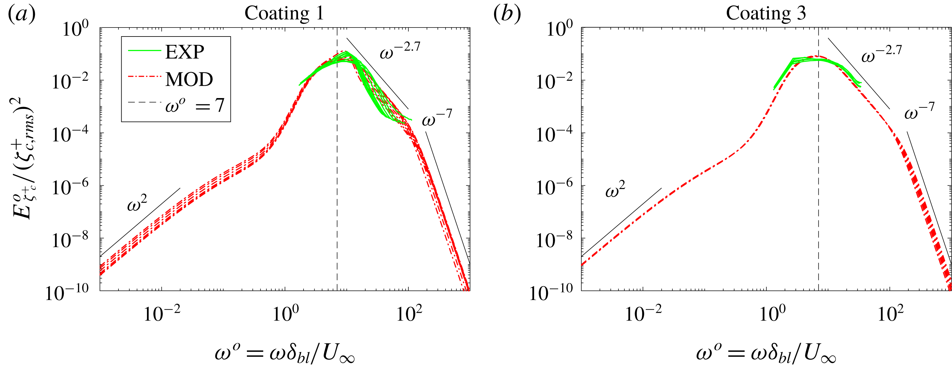


 Open access