


1. Introduction
The transition to turbulence is complex in wall-bounded shear flows. Examples include plane Couette flow (PCF), plane Poiseuille flow (PPF) and Couette–Poiseuille flow (CPF). The transition scenario in these flows is usually termed subcritical and characterised by the coexistence of turbulent and laminar regions in the transition regime. In PCF and CPF experiments where the flow is driven by a moving belt, finite amplitude background disturbances are inevitably present and we will refer to them as ‘noise’ in this article. Even if the noise is small in amplitude, the transition to turbulence occurs at values of  $Re$ that are finite and thus lower than the theoretical linear critical Reynolds number
  $Re_l$, which is infinite for PCF and CPF with zero mean flow (Klotz & Wesfreid Reference Klotz and Wesfreid2017). For plane shear flows induced by pressure gradients such as PPF, careful design of the set-up can give transition around
  $Re_l=5772$ (Orszag Reference Orszag1971) (see the definition of
  $Re$ below).
Our focus is on the transition to turbulence in plane CPF, where the flow is driven by one sided shear and the mean flux is approximately zero. It is the simplest CPF to realise experimentally (Tsanis & Leutheusser Reference Tsanis and Leutheusser1988). It can be considered as intermediate between the widely studied cases of plane Couette and plane Poiseuille flows: the main component of the motion is Couette shear with a weak return Poiseuille flow (see figure 1). We will investigate the transition process by ‘quenching’, i.e. sudden decrease in  $Re$.
$Re$.
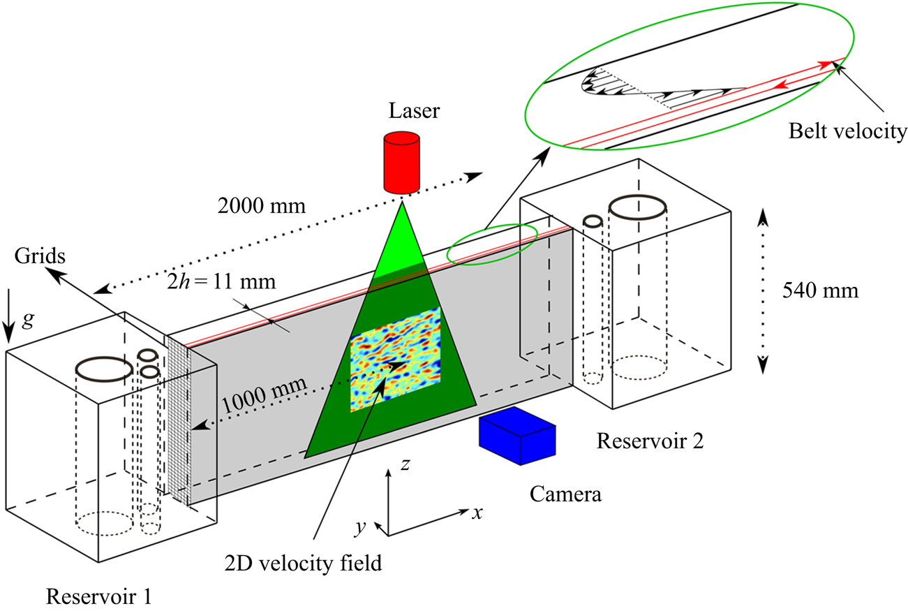
Figure 1. A schematic diagram of the experiment.
We first discuss the transition in PCF and PPF. PCF has been extensively studied experimentally and numerically. The Reynolds number is defined using the belt velocity  $U_{belt}$ and the half-gap
  $h$:
$h$:  $Re= hU_{belt}/\nu$ where
  $\nu$ the kinematic viscosity of the fluid. The global stability threshold is the Reynolds number above which the turbulent state is sustained. It is denoted by
  $Re_g$ in the present article (the notation
  $Re_c$ is also used in the literature). The value
  $Re_g=323 \pm 2$ was determined experimentally by Bottin & Chaté (Reference Bottin and Chaté1998), and
  $Re_g=324 \pm 1$ was established numerically by Duguet, Schlartter & Henningson (Reference Duguet, Schlartter and Henningson2010) in large domains. In order to avoid any arbitrariness in the choice of the lifetime for decay under quenching, the numerical work by Shi, Avila & Hof (Reference Shi, Avila and Hof2013) used an approach based on the equality of the splitting and decay rates of the turbulent regions. These are found to form banded structures in the decay regime. They found a similar global stability threshold
  $Re_g=325$ despite using a narrow tilted domain with respect to the streamwise direction introduced by Barkley & Tuckerman (Reference Barkley and Tuckerman2005). Another characteristic threshold is the Reynolds number
  $Re_t$ at which turbulence becomes featureless, which is larger than
  $Re_g$. It has been estimated experimentally as
  $Re_t=415$ by Prigent (Reference Prigent2001) and numerically as
  $Re_t=420$ by Duguet et al. (Reference Duguet, Schlartter and Henningson2010). The behaviour close to
  $Re_t$ was studied numerically in detail by Rolland (Reference Rolland2018b), showing that several cross-over Reynolds numbers can be defined close to
  $Re_t$. The transitions of laminar–turbulent bands to featureless turbulence occurs at each of the cross-over points.
The behaviour in PPF is more complex than PCF. The Reynolds number is usually defined using the centre-plane velocity of the corresponding laminar flow and the half-gap  $h$. The global threshold obtained numerically is
  $Re_g =700$ (Shimizu & Manneville Reference Shimizu and Manneville2019). This is consistent with the experimental results of PPF by Paranjape (Reference Paranjape2019), where a positive mean growth rate of the turbulent bands for
  $Re>650$ is found in quench experiments (Bottin & Chaté Reference Bottin and Chaté1998; De Souza, Bergier & Monchaux Reference De Souza, Bergier and Monchaux2020). Several cross-over Reynolds numbers can be defined, linked to the existence of bands and of their orientation. A ‘lower marginal Reynolds number’
  $Re=1050$ is obtained from the linear extrapolation of the intermittency factor by Seki & Matsubara (Reference Seki and Matsubara2012). By way of contrast with PCF, the cross-over Reynolds number obtained by equating the decay and splitting rate in a tilted narrow channel (
 $Re=965$, see the numerical work by Gomé, Tuckerman & Barkley Reference Gomé, Tuckerman and Barkley2020) is different from
  $Re_g$.
Since the mean flux is approximately zero in our experiment we use the belt speed  $U_{belt}$ as the characteristic velocity. The Reynolds number can thus be defined using this and the half-gap
  $h$:
$h$:  $Re= hU_{belt}/\nu$. This configuration has not been explored in as much detail as either PCF or PPF. The threshold at which turbulence is self-sustained in experiments is estimated approximately at
  $Re\approx 670$; the turbulence becomes featureless at
  $Re\approx 780$ (Klotz et al. Reference Klotz, Lemoult, Frontczak, Tuckerman and Wesfreid2017). Since the geometry of CPF is similar to that of PCF and PPF, it is anticipated that there will be common features in the transition processes in all three flows.
An important geometric parameter is the aspect ratio, i.e. the size of the channel in the streamwise and spanwise directions relative to the half-channel width  $h$. Turbulence cannot be sustained below a size called the ‘minimal flow unit’ (Jiménez & Moin Reference Jiménez and Moin1991; Hamilton, Kim & Waleffe Reference Hamilton, Kim and Waleffe1995), where the width and height are a few
  $h$ in wall-bounded flow. The influence of the aspect ratio has been investigated numerically in PCF by Philip & Manneville (Reference Philip and Manneville2011) and Rolland (Reference Rolland2018b). They show that the channels of sizes below around
  $80h$ only display temporal dynamics, while above
  $80h$ both spatio and temporal dynamics can be captured. For such channels, turbulent bands aligned at a well-defined angle with the streamwise direction are separated by laminar regions. The wavelength of such bands is of order
  $(70\text {--}80)h$ (Philip & Manneville Reference Philip and Manneville2011). Characteristics of flows in infinite domains are obtained in practice only for very large sizes (
 $2000h$), which have been studied using models with truncated equations (Chantry, Tuckerman & Barkley Reference Chantry, Tuckerman and Barkley2017). In this case, the turbulent fraction, defined as the ratio of the turbulent region with respect to the entire area, is a continuous function of
  $Re$ in the turbulent steady state. The minimal size of the domain required to observe complex spatio-temporal behaviours in CPF is not yet known. The aspect ratio of our experiment is sufficiently large to observe oblique bands.
As noted above, one way to study the properties of turbulence is to investigate its decay using quench experiments, i.e. the transition from turbulent to laminar flow (Batchelor & Townsend Reference Batchelor and Townsend1948; Bottin & Chaté Reference Bottin and Chaté1998; Prigent & Dauchot Reference Prigent and Dauchot2005; Peixinho & Mullin Reference Peixinho and Mullin2006; Rolland Reference Rolland2015; Paranjape Reference Paranjape2019). The advantage of the quench protocol is that the flow is initialised in the fully turbulent state, which is less sensitive to external noise than the laminar state. Changing the flow rate rapidly is challenging experimentally in Poiseuille flows, but it is relatively straightforward in our experiment where the flow is driven by a belt.
We have carried out an experimental investigation of the decay of the streamwise and spanwise components of the velocity field and highlight their roles in the relaminarisation process. In addition, these two components provide information concerning the structures that drive the self-sustained cycle of turbulence (Waleffe Reference Waleffe1997): on the one hand, the modulation of the streamwise velocity gives rise to the structures called streaks, and on the other hand, the spanwise velocity characterises the dynamics of streamwise vortices – also called rolls – which accompany the streak dynamics.
The difference in behaviour of these two components has been discussed by several authors: in a simplified model used by Rolland (Reference Rolland2018a), the proxies for the streamwise and spanwise components display different behaviours. The different decay rates of the velocity components during turbulent decay described in this work also received attention in the recent numerical work by Gomé et al. (Reference Gomé, Tuckerman and Barkley2020). The different behaviours associated with the various flow components have also been investigated in the permanent regime by Duriez, Aider & Wesfreid (Reference Duriez, Aider and Wesfreid2009) for a flat-plate boundary layer.
In the current investigation, the decay of the streamwise and spanwise velocities is carried out over a large range of Reynolds numbers, ranging from approximately half to slightly larger than  $Re_g$. This is in contrast with many previous studies, which focus on values of
  $Re$ very close to or slightly above
  $Re_g$. We aim at showing that the decay rate difference is observed over a wide range of
  $Re$, and that the global threshold
  $Re_g$ is close to the value extrapolated from the value of the decay rate at small
  $Re$. Another objective of the present study is to investigate the interplay between the rolls and streaks in the flow, in particular to elucidate the dynamics of each component.
In our Couette–Poiseuille set-up, noise is generated in the fluid supply tank and disturbed flow is thus injected into one end of the channel (see figure 1). Similar behaviour is observed in experiments on torsional Couette flow (Le Gal et al. Reference Le Gal, Tasaka, Cros and Yamaguchi2007) and PPF (Sano & Tamai Reference Sano and Tamai2016). Disordered flow may penetrate the flow field from both end tanks in CPF, since our experiment has a supply tank at each end (Couliou & Monchaux Reference Couliou and Monchaux2015). Contrary to the case of boundary layer flows, which is another example of highly sheared flow where the effect of noise has been investigated (Fransson, Matsubara & Alfredsson Reference Fransson, Matsubara and Alfredsson2005; Kreilos et al. Reference Kreilos, Khapko, Schlatter, Duguet, Henningson and Eckhardt2016), it is not common to vary the noise in channel flows. Here we characterised the noise and controlled it using grids.
The article is organised as follows. We present the main features of the experimental set-up, the velocity measurements and the processing steps in § 2. The spatial structure of the velocity fields during the relaminarisation process, as well as the temporal evolution of characteristic integral parameters such as kinetic energy and turbulent fraction, are discussed in § 3. The noise is characterised and quantified in § 4, using the velocity field in the permanent regime. The variation with Reynolds number of the characteristic decay times is discussed in § 5.
2. Experimental set-up and processing
2.1. Experimental set-up
A schematic diagram of the apparatus is shown in figure 1. It has previously been described in detail by Klotz et al. (Reference Klotz, Lemoult, Frontczak, Tuckerman and Wesfreid2017). It consisted of two parallel vertical glass plates set 14 mm apart and these form a connected channel between two filled water reservoirs. The glass plates were closed at the top and at the bottom by two horizontal surfaces, forming a channel. The tops of the reservoirs were not closed. The set-up was filled with water at room temperature  $21.5 \pm 1.5\,^\circ \textrm {C}$ and the viscosity of the water was evaluated at the measured water temperature.
The belt was a Mylar membrane which was guided by vertical cylinders so that it was parallel to the vertical glass plates, and close to one of the plates. One of the cylinders in reservoir 1 rotates, which produces a translation motion of the membrane at constant velocity  $U_{belt}$.
The flow of interest was in the widest gap between the moving membrane and the fixed glass plate. For consistency with previous investigations, the width of this gap is defined as  $2h$, where
  $2h=11.0 \pm 0.3\ \textrm {mm}$. The belt velocity
  $U_{belt}$ created a shear flow which also induced a pressure difference between the two reservoirs. This pressure difference created a counter flow, so that the mean flow was almost zero in the wall-normal
  $y$ direction. A parabolic (Couette–Poiseuille) profile was obtained in the laminar regime.
The length of the channel in the streamwise direction, i.e. the  $x$ direction, is
  $L_x=2000\ \textrm {mm}$, so that
  $L_x/h=364$. The height of the channel in the spanwise direction, i.e. the
  $z$ direction, is
  $L_z=540\ \textrm {mm}$, so that
  $L_z/h=98$. The half-channel width
  $h$ and the belt velocity
  $U_{belt}$ are used to make the variables dimensionless. The Reynolds number is defined as
  $Re=U_{belt}h/\nu$, where
  $\nu$ is the kinematic viscosity of water with
  $\nu \in [0.934, 1.003]\ \textrm {mm}^{2}\ \textrm {s}^{-1}$ in our experiments. The
  $U_{belt}$ was in the range of
  $[0.03, 0.2]\ \textrm {m}\ \textrm {s}^{-1}$ in our study. In the following of the article, we will denote dimensional parameters by an asterisk exponent.
The rotating cylinder in reservoir  $1$ which drove the belt induced a large-Reynolds-number turbulent flow in the reservoir. At
  $Re=600$ in the channel, the
  $Re$ in reservoir
  $1$ was approximately
  $2\times 10^4$ which is calculated using the half-width of the reservoir
  $H^*=23\ \textrm {cm}$ and
  $U_{belt}$. This source of turbulence acted as external noise for the flow inside the channel. Some of the turbulence generated in the reservoirs invaded the flow channel as reported in PCF experiments (Bottin & Chaté Reference Bottin and Chaté1998; Couliou & Monchaux Reference Couliou and Monchaux2015).
A novelty of the present experiment was the addition of multi-layer grids at the junction between reservoir 1 and the channel to help reduce the noise that perturbs the flow in the channel. Fine mesh grids have previously been used in boundary layer flows to reduce the streaky flow and homogenise the incoming flow (Puckert, Dieterle & Rist Reference Puckert, Dieterle and Rist2017). The multi-layer grids consisted of  $5$ stainless steel grids with a distance between the layers of 1–2 mm. The diameter of the wires was 0.4 mm. The size of the grids was
  $25\ (\textrm {width}) \times 500\ (\textrm {height})\ \textrm {mm}$. The mesh size 1 mm was significantly smaller than
  $2h$ and breaks up the large eddies and prevents them from entering the channel. It was found that the level of noise in the channel was sensitive to the exact position of the grid. We studied four levels of external noise: one without the grid (high noise) and three with the grid in place.
2.2. Particle image velocimetry
Two-dimensional particle image velocimetry (PIV) was used to measure the velocity field in the  $x-z$ plane. The location of this plane in the
  $y$ direction was
  $y=0.33\pm 0.04$, which is the position where the velocity passes through zero in the laminar profile (see figure 5(
 $b$) (Klotz et al. Reference Klotz, Lemoult, Frontczak, Tuckerman and Wesfreid2017)). This plane was selected using a laser sheet obtained from a Darwin-Duo
 $^{\circledR }$ 20 mJ Nd-YLF double-pulse green laser (527 nm). The time interval between the two laser pulses was
  $\Delta t^* = 12.5\ \textrm {ms}$ and the pulse duration was less than
  $250$ ns. The fluid was seeded to enable PIV with particles of diameter
  $20\ \mathrm {\mu }\textrm {m}$ made of polyamide (density
  $1.03\ \textrm {g}\ \textrm {cm}^{3}$) with a volume concentration of
  $1.7\times 10^{-5}\ \textrm {g}\ \textrm {ml}^{-1}$.
Images were acquired using a camera Imager MX5M $^{\circledR }$ from LaVision
 $^{\circledR }$ (
 $2464 \times 2056$ pixels) with a frequency
  $f^*=2\ \textrm {Hz}$ using the double frame mode. The time duration between two consecutive frames was set as the interval between two laser pulses. A Nikon
 $^{\circledR }$ objective lens 17–35 mm with an aperture
  $f/2.8$ was mounted with a distance 920 mm from the measurement plane. The field of view was fixed at the middle of the channel, around
  $180h$ between the centre of the measurement field and the entrance of the channel from the reservoir
  $1$ side (see figure 1). The size of the measurement field was
  $77h \times 79h$.
The velocity fields were computed using DaVis 10 software (LaVision) with a multi-pass algorithm. As the velocity field was dominated by the streamwise velocity component, the displacement of the particles in this direction was more than one order of magnitude larger than the spanwise. Therefore, we used an interrogation window which is elliptical with an aspect ratio  $4:1$ between the streamwise and spanwise directions. The total number of pixels of this interrogation windows is
  $2304$, and the overlap between two successive windows is
  $50\,\%$. As the PIV calculation induces some artifacts close to the boundary of the measured field, the velocity field was cropped to a size of
  $65h\times 67h$.
2.3. Protocol
The following protocol was used in the experiments: the flow was initialised at  $Re_i = 1000 > Re_t$, i.e. in the featureless turbulent regime. The belt speed was then suddenly reduced to the lower final Reynolds number
  $Re_f$. This protocol is commonly referred to as a quench experiment (Bottin & Chaté Reference Bottin and Chaté1998; De Souza et al. Reference De Souza, Bergier and Monchaux2020). The decrease of the Reynolds number was achieved by decreasing the velocity of the membrane, using a Labview program controlling the rotation of the motor as a function of time. The time required to change the belt velocity is less than 0.1 s, i.e. at most
  $2$ time units (
 $h/U_{belt}$). This time is much smaller than the typical decay time of the turbulence in the channel. In the following, time
  $t=0$ corresponds to the time at which the Reynolds number is decreased.
2.4. Small scales
The velocity  $U$ can be decomposed into
  $U = u_{lsf}+u$, where
  $u_{lsf}$ is the large-scale flow (LSF) and
  $u$ is the small-scale flow (SSF). LSFs in wall-bounded shear flows arise from the non-zero spanwise velocity component (Duguet & Schlatter Reference Duguet and Schlatter2013), and a small contribution from the imperfections of the membrane in the channel. The scale separation in the present set-up was investigated by Klotz, Pavlenko & Wesfreid (Reference Klotz, Pavlenko and Wesfreid2021).
In this investigation, we remove the LSF and focus on the SSF  $u$, which is the most significant contribution to the turbulent flow field (Lemoult, Aider & Wesfreid Reference Lemoult, Aider and Wesfreid2013). We used a two-dimensional fourth-order Butterworth spatial filter with a cutoff wavelength
  $\lambda \leq 14.8$ to remove LSFs. The wavelength
  $\lambda$ is defined as
  $2{\rm \pi} /\lambda =k=\sqrt {k_x^{2}+k_z^{2}}$, where
  $k_x$ and
  $k_z$ are the streamwise and spanwise wavenumbers, respectively. The results do not change qualitatively when
  $\lambda$ is varied between
  $8.4$ and
  $16.8$. For example, the decay time
  $\tau$ (defined in § 5) changed by less than
  $5\,\%$ for measurements at final Reynolds number
  $Re_f=500$. The small-scale velocity fluctuation
  $u_x$ is a measure of the streaks and the spanwise velocity
  $u_z$ corresponds to the streamwise vortices, also termed rolls.
2.5. Energy and turbulent fraction
We characterise the global state of the flow in the field of view using both kinetic energies and turbulent fractions. To investigate possible different behaviours of the velocity in the streamwise ( $u_x$) and spanwise (
 $u_z$) directions, we define variables which only depend on either of these velocity components. We recall that
  $u_x$ is one order of magnitude larger than
  $u_z$. This approach was used by Klotz & Wesfreid (Reference Klotz and Wesfreid2017) for the study of transient growth in CPF.
We define the streamwise ‘perturbation energy’  $E_{x}$ as
 \begin{equation} E_{x} = \frac{1}{2L_xL_z}\int_{{-}L_z/2}^{L_z/2} \int_{0}^{L_x}{u_x}^2\,\textrm{d}x\,\textrm{d}z. \end{equation}
Similarly, we define the spanwise energy of the rolls  $E_{z}$ as
 \begin{equation} E_{z} = \frac{1}{2L_xL_z}\int_{{-}L_z/2}^{L_z/2} \int_{0}^{L_x}{u_z}^2\,\textrm{d}x\,\textrm{d}z. \end{equation}
Since we use a non-dimensional quantity, the density of the fluid is not explicitly involved in the definition of the energy.
Several methods have been used to estimate the turbulent fraction of the flow field defined as the fraction of space where the flow is turbulent. Experimentally or numerically, the velocity is often non-zero even in the laminar regions. Hence, there is some arbitrariness in the choice of the variable which is used to define the turbulent fraction, as well as in the choice of the threshold.
Pioneering experiments on PCF used visualisation of the flow with anisotropic Iriodin particles (see Daviaud, Hegseth & Bergé Reference Daviaud, Hegseth and Bergé1992; Tillmark & Alfredsson Reference Tillmark and Alfredsson1992; Bottin & Chaté Reference Bottin and Chaté1998). This is an indirect characterisation of the local velocity field. The energy averaged on a cell size close to that of the minimal flow unit has been used in the numerical work of Rolland & Manneville (Reference Rolland and Manneville2011). The streamwise velocity is the dominant contribution to the energy, and thus to the latter definition of the turbulent fraction. In their experimental work, De Souza et al. (Reference De Souza, Bergier and Monchaux2020) use a method based on the measurement of the normal vorticity. Despite these differences, the qualitative variation of the turbulent fraction with time or Reynolds number is consistent.
Since we focus on the flow structures of the turbulent flow, we chose to define two ‘turbulent fractions’. The turbulent fraction  $F_x$ is computed from the streamwise velocity: a point is considered as turbulent if
  $|u_x| >1.4 \times 10^{-2}$. This value was obtained by comparing the velocity field and the turbulent region after thresholding. The typical
  $|u_x|$ of the streaks is around
  $6\times 10^{-2}$. Similarly, we define
  $F_z$ using the spanwise velocity only: a point is considered as turbulent if
  $|u_z| >7 \times 10^{-3}$. The typical
  $|u_z|$ of the rolls is around
  $3\times 10^{-2}$.
3. Decay process
We outline typical features of the decay processes found in quench experiments using the results from two representative cases: one at  $Re_f=425$, which is far below
  $Re_g$, and a second at
  $Re_f=600$, which is closer to this threshold. We also investigate the influence of the final Reynolds number on the decay process.
Velocity fields for different times are shown in figure 2 for a  $Re_f=425$ experiment: the top row (
 $a$–
$a$– $d$) and bottom row (
 $e$–
$e$– $h$) show, respectively, the streamwise
  $u_x$ and spanwise
  $u_z$ fields. Figures 2(
 $a$) and 2(
 $e$) are respectively the streamwise and spanwise velocity fields before the quenching, i.e. when the Reynolds number is
  $Re_i=1000$. As expected, the flow is fully turbulent. The streaks can be identified as the elongated structures aligned in the
  $x$ direction in figure 2
 $(a)$. These streaks have a typical length of
  $(10\text {--}20)h$, and are typically not straight as in this figure. The velocity field
  $u_z$ displayed in figure 2
 $(e)$ is irregular, as expected for a turbulent flow. The magnitude of
  $u_z$ is one order of magnitude smaller than for
  $u_x$, which is a common feature of three-dimensional flow structures in wall-bounded shear flows.
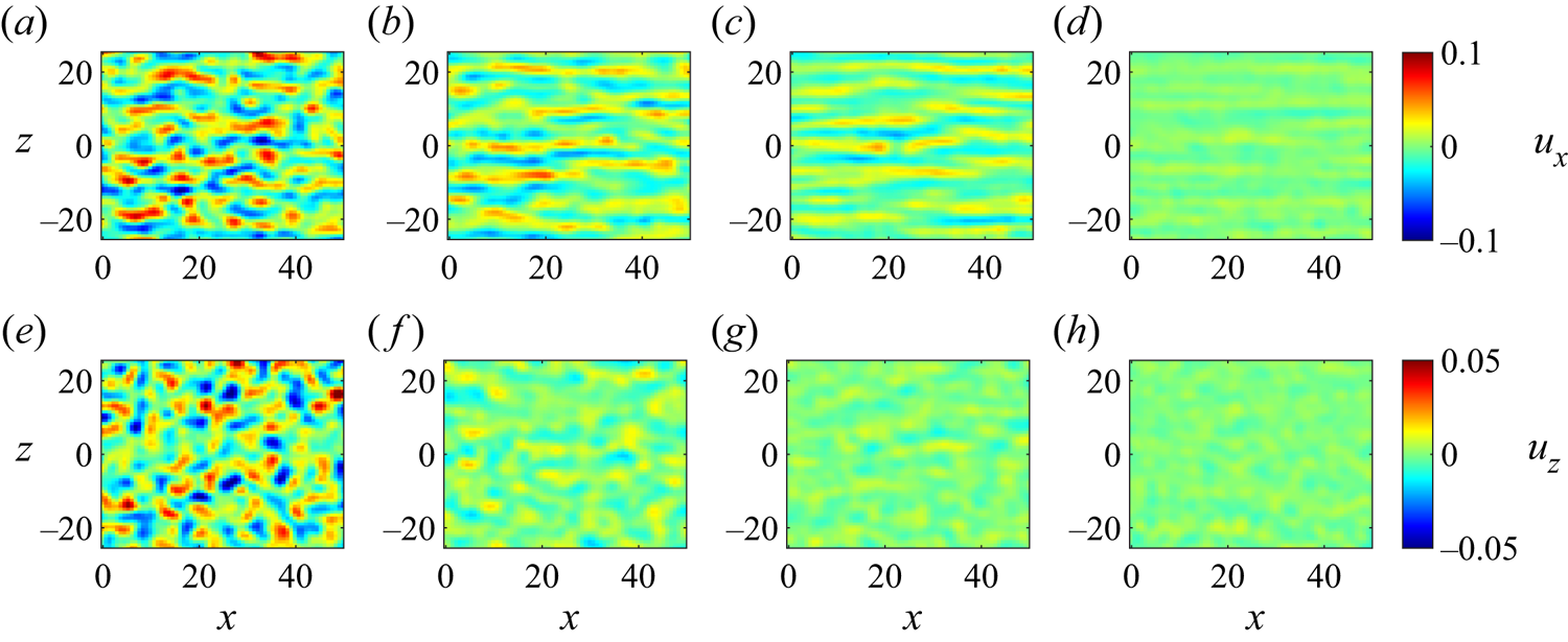
Figure 2. Snapshots of velocity fields for different times at  $Re_f=425$. (a–d) Velocity fields in the streamwise direction
  $u_x$, (e–h) velocity fields in the spanwise direction
  $u_z$. Times: (
 $a$,
$a$, $e$)
$e$)  $t=-65$ (fully turbulent flow,
  $Re_i=1000$), (
 $b$,
$b$, $f$)
$f$)  $t=91$, (
 $c$,
$c$, $g$)
$g$)  $t=150$, (
 $d$,
$d$, $h$)
$h$)  $t=286$; noise intensity: high (
 $\sigma =4.6\times 10^{8}$, defined in § 4.1).
A typical evolution of the decay of turbulence at three successive time instants is displayed in figures 2( $b$–
$b$– $d$) and 2(
 $\,f$–
 $h$). The velocity fields of
  $u_x$ after the quench are shown in figure 2(
 $b\text {--}d$). The streaks become longer and broader. The corresponding
  $u_z$ velocity fields are shown in figure 2(
 $\,f\text {--}h$). The decay of
  $u_z$ is faster than
  $u_x$, as can be seen for example at
  $t=150$, by comparing figure 2(
 $c$,
$c$, $g$) and the shape of the structures in the
  $u_z$ field does not change significantly. The decay of the velocity field of
  $u_x$ is different from that of
  $u_z$. This decay scenario of streaks is qualitatively similar to that found in numerical simulations of PCF (Philip & Manneville Reference Philip and Manneville2011). This was attributed by them to a viscous damping effect and is typical for decaying turbulence (Batchelor & Townsend Reference Batchelor and Townsend1948).
The temporal energy evolution for the streamwise component  $E_{x}$ is shown in figure 3(
 $a$) and the spanwise component
  $E_{z}$ in figure 3(
 $b$). Note that the abscissa is linear, whereas the ordinate is displayed on a logarithmic scale. The dashed vertical black lines indicate the times at which the corresponding velocity fields are plotted in figure 2 to illustrate the dynamics of streaks and rolls. The magnitude of the energy depends on the wall-normal
  $y$ position of the measured field (see § 2.2). The uncertainties of the position can change the absolute value of the measure but this does not have a significant influence on the results. In this example, the energies decrease monotonically, which is linked to the small value of the Reynolds number. The value of
  $E_z$ decreases faster than the
  $x$-component, in agreement with the observation discussed above with reference to figure 2. We observed two different decay stages in the evolution of
  $E_x$ after the quench: (i)
  $t\lesssim 160$, the decay accompanied by elongating and flattening of streaks, which corresponded to the snapshots in figure 2(
 $b$,
$b$, $c$); (ii)
  $t\gtrsim 160$, fading of streaks induced by viscous damping, which corresponded to the snapshots from figures 2(
 $c$) to 2(
 $d$).
$d$).
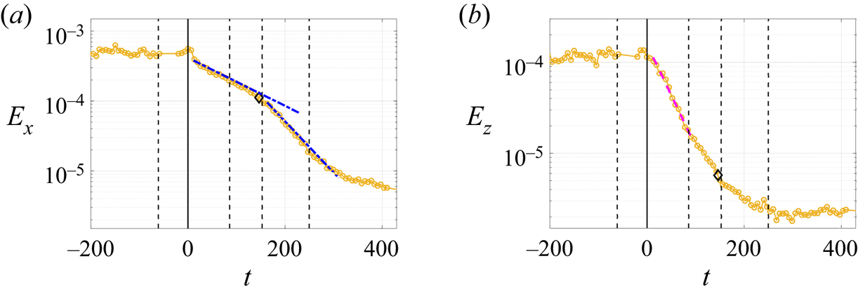
Figure 3. Temporal evolution of  $E_{x}$ (
 $a$) and
  $E_{z}$ (
 $b$) for
  $Re_f=425$; dashed vertical lines represent the times for the snapshots of
  $u_x$ and
  $u_z$ plotted in figure 2; blue dot-dashed lines: guide for the eyes to distinguish the different decay stages for
  $E_x$; magenta dashed line: exponential fits
  $E_{z}=E_0\exp (A_zt)$; black diamond: the position of
  $\tau _z$ when
  $E_z$ decreases to
  $5\,\%$ of its initial energy; noise intensity: high (
 $\sigma =4.6\times 10^{8}$, defined in § 4.1).
We also compared the decays of  $E_x$ and
  $E_z$ and found that
  $E_z$ is negligible during the second stage of the decay of
  $E_x$. To quantify this, we define the decay time
  $\tau _z$ at which the energy
  $E_z$ decreases to
  $5\,\%$ of its initial value
  $E_i$. The choice of the threshold for the definition of
  $\tau _z$ will be discussed in § 5. The data point at
  $\tau _z$ is plotted as a black diamond in figure 3(
 $a$,
$a$, $b$). We can see in figure 3(
 $a$) that
  $\tau _z$ is close to the time when the decay of
  $E_x$ becomes faster, i.e. changes from one stage to another. This can be explained by the observation that rolls are present during the first stage of the decay, but have a negligible amplitude in the second stage (after
  $\tau _z$). The rolls generate streamwise perturbations in the form of streaks, which is called the lift-up effect (Schmid & Henningson Reference Schmid and Henningson2001). The decay of the streamwise component is sensitive to the presence of the other components. This effect has been discussed in particular in Rolland (Reference Rolland2015) who expresses the energy budget during the quench (equation (9)) as the sum of a term linked to the interaction between streaks and rolls, and a term associated with the viscous dissipation of the streaks.
The magenta dashed line in figure 3( $b$) represents an exponential fit of the function
 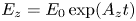 $E_z=E_0\exp (A_zt)$, where
  $A_z$ is the decay rate of
  $E_z$ and
  $E_0$ is the initial energy. This illustrates that the energy
  $E_{z}$ decays exponentially under quenching. We initiated the fit
  $2$ data points (approximately
  $\Delta t\in [9,16]$) after
  $t=0$ to obtain a better fit as it reduces the sum of the squared residuals. This exponential fit covers approximately one decade of energy. The decay rate
  $A_z$ is linked to the decay time
  $\tau _z$ by the relation
 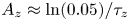 $A_z \approx \ln (0.05)/\tau _z$ (the decay of
  $E_z$ is not perfectly exponential, so the equality is only approximate).
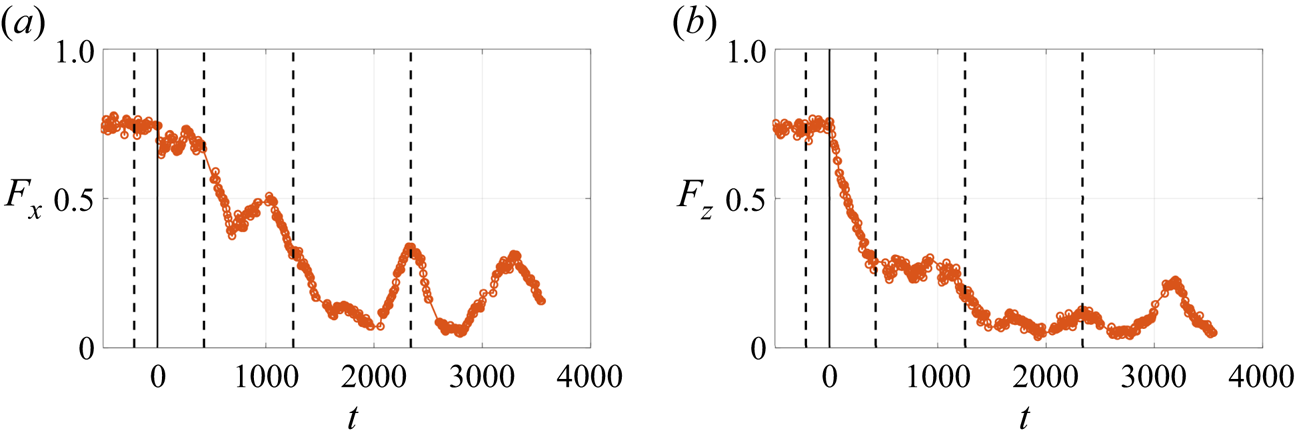
The turbulent fractions  $F_x$ and
  $F_z$ are plotted as a function of time in figure 4. The decay of
  $F_x$ also contained evidence for two different stages. We fit the decay of
  $F_z$ and the second decay stage of
  $F_x$ by a linear function
  $F_i = a_it+b$ (
 $i=x,z$). The best fit of the second slope
  $a_{x}$ of
  $F_x$ was obtained from a point just after
  $\tau _z$ to the time when the minimal slope was found with a minimum
  $12$ data points fitted. As a result of the limited data range of the second decay stage of
  $F_z$, both linear and exponential relationships provide acceptable fits. For consistency and simplicity in the rest of the paper, we use a linear fit. The fits for the decay rate
  $A_z$ and decay slope
  $a_i$ are performed on 5 realisations, separately. The average and standard deviation of their values are presented and discussed in § 5.
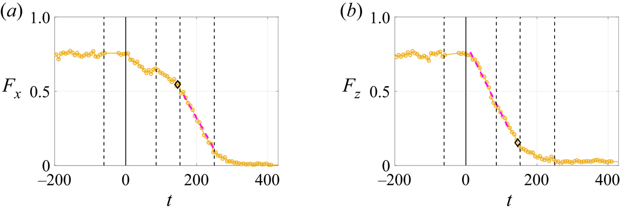
Figure 4. Temporal evolution of  $F_x$ (
 $a$) and
  $F_z$ (
 $b$) for
  $Re_f=425$; dashed vertical lines represent the times for the snapshots of
  $u_x$ and
  $u_z$ plotted in figure 2; magenta dashed lines: linear fits
  $F_{i}= a_{i}t+b$, (
 $i=x,z$); black diamond: the position of
  $\tau _z$ when
  $E_z$ decreases to
  $5\,\%$ of its initial energy; noise intensity: high (
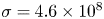 $\sigma =4.6\times 10^{8}$, defined in § 4.1).
The decay slope  $a_{x}$ is greater than
  $a_z$, which means the rolls decay faster than the turbulent and laminar streaks. The change of slopes with
  $Re_f$ will be discussed in § 5. One hypothesis of linear decay of turbulent fraction is the formation of laminar holes and the linear increase of laminar region (Rolland Reference Rolland2015). As Rolland (Reference Rolland2015) notes, numerical simulations of quenches in PCF show that the decay is exponential for the kinetic energy and linear for the turbulent fraction
  $F_t$ in the range
  $(Re_g,Re_t)$. We found linear decay is also valid for
  $Re_f < Re_g$. In addition, the two decay regimes of the streaks were revealed.
The equivalent plots to figures 2, 3 and 4 are shown in figures 5, 6 and 7 for the case of  $Re_f=600$. It can be seen in figure 6 that
  $E_{x}$ and
  $E_{z}$ suddenly decrease, which indicates that the flow has changed to a less turbulent state (smaller
  $F_x$). As the decay is rapid and the number and range of data points is limited, an exponential fit does not provide a good fit to the data. On the other hand, the decay times
  $\tau _x$ and
  $\tau _z$ are always well defined and can be used to quantify the decay over a wide range of Reynolds numbers. Therefore, we used them in § 5 to study the influence of
  $Re_f$ on the decay process.
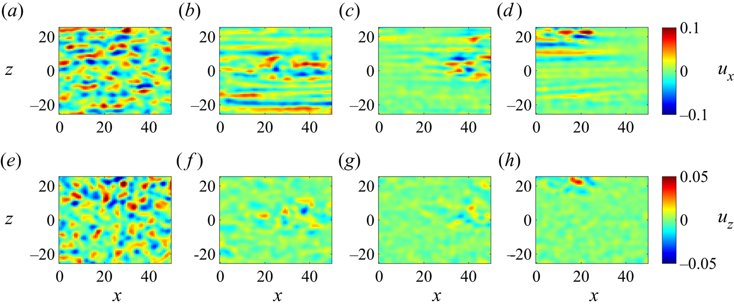
Figure 5. Snapshots of  $u_x$ (a–d) and
  $u_z$ (e–g) at different times for
  $Re_f=600$: (
 $a$,
$a$, $e$)
$e$)  $t=-215$, (
 $b$,
$b$, $\,f$)
  $t=430$, (
 $c$,
$c$, $g$)
$g$)  $t=1255$, (
 $d$,
$d$, $h$)
$h$)  $t=2430$; noise intensity: high (
 $\sigma =4.6\times 10^{8}$, defined in § 4.1).
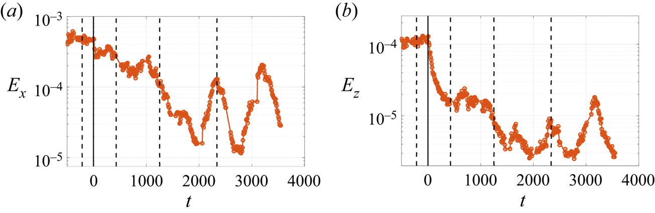


After some time, the turbulent patches were advected away from the measurement window towards reservoir  $2$ (see figure 5
 $c$,
$c$, $g$). We also observed that the streaks can re-enter the observation area from reservoir
  $1$. This can be observed in the snapshots of figure 5(
 $d$,
$d$, $h$) and help explain the local maximum in energy at
  $t\approx 2430$ in figure 6. We will discuss these effects in detail in § 4.2, where we show that the first stage of the decay discussed here is not affected by this noise.
The snapshots of  $u_x$ and
  $u_z$ at
  $Re_f=600$ shown in figure 5 illustrate a different decay scenario from the
  $Re_f=425$ case. The temporal evolution of
  $F_x$ and
  $F_z$ for
  $Re_f=600$ is shown in figure 7 plotted on a linear–linear scale. The turbulent fraction evolution is close to the energy evolution at
  $Re_f=600$. After quenching, as in figure 5(
 $b$), it can be seen that the streaks in the lower half-part of the measurement window become elongated and straighten, in contrast to the turbulent streaks in the middle. At the same time, the rolls in the lower part become weak and the flow is approximately laminar. This means the long straight streaks cannot reinject energy into rolls. This observation is consistent with the mechanisms of reinjection of energy into the rolls driven by nonlinear interactions between wavy streaks (Waleffe Reference Waleffe1997). The patch of streaks and rolls are subsequently advected by the moving wall towards reservoir
  $2$ as in figure 5(
 $c$). In figure 5(
 $d$), the streaks and rolls re-enter the measured field from the left side (i.e. from reservoir
  $1$).
$1$).
In order to investigate the influence of lift-up effect for different  $Re_f$, the energy evolution of
  $E_x$ and
  $E_z$ and the turbulent fraction evolution of
  $F_x$ and
  $F_z$ for three different final Reynolds numbers,
  $Re_f=300$,
  $Re_f=425$ and
  $Re_f=500$, are compared in figure 8 and 9. The change of decay regime is not observed in the evolution of
  $E_x$ and
  $F_x$ for
  $Re_f=300$. This implies the lift-up effect at this small Reynolds number is not pronounced. As
  $Re_f$ increase to
  $425$, we observe the existence of two decay stages. With the further increase of
  $Re_f$ to
  $500$, we observe that the energy
  $E_x$ and turbulent fraction
  $F_x$ first drop to a lower plateau after the quench and the plateau is maintained until approximately
  $\tau _z$ when
  $E_z$ and
  $F_z$ decay to very low levels. This transient plateau is a result of the lift-up mechanism and the roll is a key ingredient. When the roll is no longer active, the plateau is not sustained.
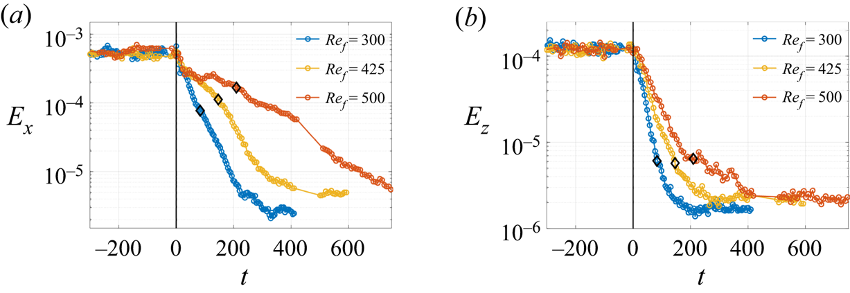
Figure 8. Temporal evolution of  $E_x$ (
 $a$) and
  $E_z$ (
 $b$) for
  $Re_f=300$,
  $425$ and
  $500$; black diamonds:
  $\tau _z$ for each
  $Re_f$; noise intensity: high (
 $\sigma =4.6\times 10^{8}$, defined in § 4.1).
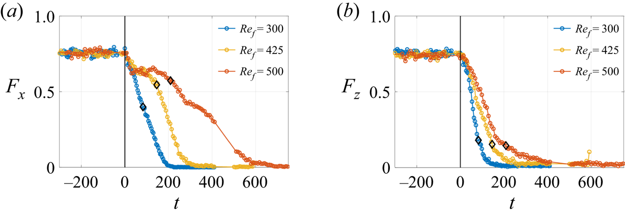
Figure 9. Temporal evolution of  $F_x$ (
 $a$) and
  $F_z$ (
 $b$) for
  $Re_f=300$,
  $425$ and
  $500$; black diamonds:
  $\tau _z$ for each
  $Re_f$; noise intensity: high (
 $\sigma =4.6\times 10^{8}$, defined in § 4.1).
In summary, we have uncovered important details of the decay process at  $Re_f=425$ and
  $Re_f = 600$, respectively. The decay of turbulence is direct throughout the flow field at
  $Re_f=425$, in contrast to a partial decay or a formation spatially distinct laminar holes at
  $Re_f=600$. We made the observation that the decay rates and decay slopes are different by comparing the decays of the streamwise energy
  $E_x$ and the turbulent fraction
  $F_x$ with the spanwise energy
  $E_z$ and the turbulent fraction
  $F_z$, respectively. The decay of the streamwise component revealed two different decay stages depending on the presence of the roll component, which is an important ingredient of the lift-up effect.
4. Noise
4.1. External noise in the permanent regime
Noise is inevitably present in the experiment since there is a rotating cylinder driving a moving belt through a reservoir. Here, we have varied the noise level using grids at the entrance to reservoir  $1$. The efficiency of the grids depends on the mechanical mount supporting them and this was found to have a significant effect on the level of noise. In this section, we discuss measurements to illustrate that the level of noise could be controlled and quantified. The quantification is indirect, since the velocity field is the response of the flow field to the external noise. As mentioned in § 3 and in the work of Kreilos et al. (Reference Kreilos, Khapko, Schlatter, Duguet, Henningson and Eckhardt2016) for boundary layer flow, the turbulent state is only observed when the
  $z$ component is significant. In the following, the noise levels are quantified using the roll component.
The time averaged spanwise energy of the permanent state is
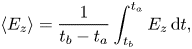 \begin{equation} \langle E_{z}\rangle = \frac{1}{t_b-t_a}\int_{t_b}^{t_a} E_{z}\,\textrm{d}t, \end{equation}
where  $t_a$ is the time when the transient decay ends after quenching,
  $t_b$ is the end of the measurement. We used
  $t_a=1500 > t_{adv}$, where
  $t_{adv}$ is the advection time during which the streaks travel from the entrance to the channel past the measured station (see § 4.2). In order to ensure the average started after the transient decay,
  $\langle E_{z}\rangle$ is approximately a constant when the time span is
  $t_b-t_a>5 \times 10^3$. The variance of the permanent state is defined by
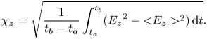 \begin{equation} \chi_{z} = \sqrt{\frac{1}{t_b-t_a}\int_{t_a}^{t_b} ({E_{z}}^2-{<}E_{z}>^2)\,\textrm{d}t}. \end{equation}
A plot of  $\langle E_{z}\rangle$ as a function of
  $Re_f$ for the four different noise levels is given in figure 10(
 $a$). The red points correspond to the experiments without grids, i.e. for which the noise is the greatest. The three other colours correspond to three different positions of the grid. The time averaged
  $\langle E_z\rangle$ is linked to both the dynamics and the noise level and provides a measure of the response of the flow to the noise.

Figure 10.  $(a)$ Time and space averaged amplitude
  $\langle E_{z}\rangle$ of the final state as a function of
  $Re_f$ for different noise levels; error bar: standard deviation of 5 realisations for red and green data, 2 realisations for yellow and blue data.
  $(b)$ Variance
  $\chi _z$ of the final state for different noise levels; black dot-dashed lines: guide for the eyes.
The different curves have a similar shape but are shifted along the  $Re_f$ axis. The laminar state is linearly stable in this system and the noise is amplified through transient growth (Klotz & Wesfreid Reference Klotz and Wesfreid2017). It is thus expected that the greater the noise level, the higher the energy of the flow at a given
  $Re_f$. From the figure, we rank the datasets high to low: red, yellow, green, blue, respectively. We observed that the flow remains laminar at
  $Re_f=680$ for the blue curve, i.e. the lowest noise level.
We also characterised the noise using the variance. The idea of using the variance is inspired by the use of susceptibility (see for instance García-Ojalvo & Sancho Reference García-Ojalvo and Sancho1999), where the external field would be replaced here by the noise. It is also inspired by Agez et al. (Reference Agez, Clerc, Louvergneaux and Rojas2013) and Rolland (Reference Rolland2018b), who uses response functions to characterise bifurcations in PCF. The noise is intrinsic in the case of Rolland (Reference Rolland2018b), induced by the turbulence, whereas here we characterise it as an external disturbance.
The variance  $\chi _{z}$ as a function of
  $Re_f$ for the different noise levels is presented in figure 10(
 $b$). We observe that the maximum
  $\chi _{z}$ increases as the noise level decreases. Therefore, we define the inverse
  $\sigma$ of the maximum
  $\chi _{z}$ as a proxy of the noise intensity
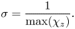 \begin{equation} \sigma = \frac{1}{\max(\chi_{z})}. \end{equation}
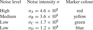
We obtain the four noise intensities and corresponding noise levels which are listed in table 1. We use the notation high ( $\sigma _A$), medium (
 $\sigma _B$) and low noise (
 $\sigma _C$ and
  $\sigma _D$) levels throughout the paper to indicate the various noise intensities defined here. The dominant frequency of the noise is close to the frequency of the belt motion loop.
Table 1. List of noise levels and intensities; marker colour refers to the colour of the data points in figures 10, 14 and 15.
The apparent threshold of CPF is shifted to higher  $Re_f$ through reducing the noise level. This observation is similar to the work by Agez et al. (Reference Agez, Clerc, Louvergneaux and Rojas2013). They use an amplitude equation model with additive noise to study the influence of the noise level on a sub-critical bifurcation. They report that the increase of the intensity of the additive noise shifts the threshold to lower values, similar to the imperfection sensitivity in shell buckling.
4.2. Advection of turbulent spots
Turbulent spots are observed in the permanent regime for Reynolds numbers close to the global stability threshold. An example of such a spot can be seen at  $Re_f=600$ in figure 5(
 $d$,
$d$, $h$). Further, its accompanying signature in the integral measurements, e.g. the clear bump around
  $t=2430$ in the turbulent fraction, is shown in figure 7. We examine now the advection of spots, which will be helpful to interpret the results in § 5 concerning the variation of characteristic times with the Reynolds number which are independent of the external noise level.
The advection of turbulent spots at  $Re_f=610$ is shown in the series of snapshots in figure 11. We observe that the spots are advected from left to right in figure 11(
 $a$–
$a$– $c$) and decay from figures 11(
 $c$) to 11(
 $d$). The observation that the streaks travel suggests that this is induced by the small mean velocity in the channel, the invasion of the turbulence and the asymmetric CPF profile. The corresponding spatio-temporal diagram of the streamwise energy averaged over the
  $z$ direction
  $\langle E_{x}\rangle _z$ is plotted in figure 12(
 $a$) in order to study the evolution of a spot. We estimate the advection velocity of streaks
  $U_{adv}$ by the slope of the white dashed lines in figure 12(
 $a$) which separates the laminar flow and the streaks. These two lines are almost parallel, which suggests that the turbulent spots are advected and decay. We can observe from the energy evolution between the white dashed lines that the decay of spots is mainly due to the decrease of the energy without an apparent reduction of the turbulent area. This corresponds to the fading trajectory and the minimal spot reported by De Souza et al. (Reference De Souza, Bergier and Monchaux2020). The value of
  $U_{adv}$ as a function of
  $Re_f$ is shown in figure 12(
 $b$). It is clear that the mean value of
  $U_{adv}$ is approximately constant with
  $\langle U_{adv}\rangle =0.13$. (red dashed line in figure 12
 $b$).
$b$).
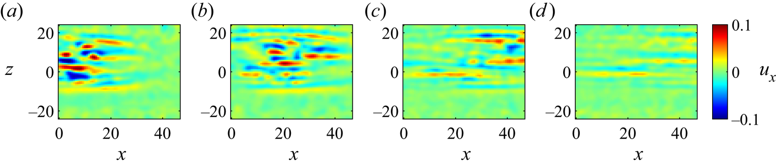
Figure 11. Snapshots of  $u_x$ at
  $(a)$
$(a)$  $t=2000$;
  $(b)$
$(b)$  $t=2100$;
  $(c)$
$(c)$  $t=2200$; and
  $(d)$
$(d)$  $t=2300$ for
  $Re_f =610$; noise level: medium (
 $\sigma _B$).
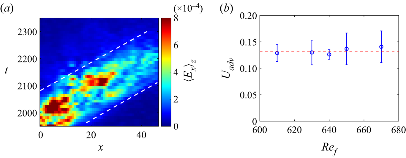
Figure 12.  $(a)$ Spatio-temporal diagram of streamwise amplitude
  $\langle E_{x}\rangle$ averaged over the
  $z$ direction for
  $Re_f=610$ in the time range
  $t\in [1900, 2350]$ during which a patch of streaks is advected in the measured field, white dashed line: the separation between laminar flow and the front of the streaks. (The diagram corresponds to figure 11.).
  $(b)$ Estimated advection velocity of turbulent streaks as a function of
  $Re_f$, blue circle: estimating
  $U_{adv}$ from the spatio-temporal diagram of
  $\langle E_{x}\rangle _z$ (the slope of the white dashed line); red dashed line: mean
 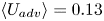 $\langle U_{adv}\rangle =0.13$ of the blue circles; error bar: standard deviation of 5 estimations.
The observation is that the main source of the external noise is the rotating cylinder in reservoir  $1$ (see figure 1). The noise generates turbulent streaks and rolls that are advected from the entrance of reservoir
  $1$ towards reservoir
  $2$. We estimated the time for the streaks to be advected from the entrance of reservoir
  $1$ to the centre of the measurement window as
 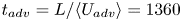 $t_{adv}=L/\langle U_{adv}\rangle =1360$. As a result, if the decay time is longer than
  $t_{adv}$, the streaks and rolls will be advected away from the measured field. The measurement of the decay time
  $\tau$ is thus limited by
  $t_{adv}$. Our measurement of the decay time is smaller than this typical time
  $t_{adv}$. This implies that the measurements are not affected by the external noise. However, the noise plays a major role in the permanent regime.
4.3. Intrinsic noise
As discussed in § 4.2, the external noise has no detectable influence on the transient decays. However, since the flow is turbulent, we observe some variability between each realisation of the quench procedure. We find that five realisations of each quench are sufficient to enable a meaningful average decay time.
The energy evolution of the streamwise component (streaks)  $E_{x}$ is shown in figure 13(a,c,e) and the spanwise component (rolls)
  $E_{z}$ in (b,d,f) for
  $20$ repeated realisations for
  $Re_f=375$,
  $510$ and
  $525$ with low noise level (
 $\sigma _C$). The energy evolution of
  $E_{z}$ is repeatable for
  $Re_f=375$. For the instance in figures 13(
 $a$) and 13(
 $b$), the relative variations (ratio of the standard deviation to the mean value) of
  $\tau _x$ and
  $\tau _z$ are
  $9\,\%$ and
  $8\,\%$ for
  $Rey_f=375$, respectively. When
  $Re_f>500$, the energy evolution of
  $E_{x}$ begins to spread and is different for each realisation. The relative variations of
  $\tau _x$ and
  $\tau _z$ are
  $31\,\%$ and
  $26\,\%$ for
  $Re_f=525$ in figures 13(
 $e$) and 13(
 $\,f$), respectively. The spread of the realisations increases with
  $Re_f$. However, even at the highest
  $Re_f$, the spread is small. Note that this decay time is different from the lifetimes obtained from the probability distribution of the relaminarisation times, which is wide close to
  $Re_g$ (Grebogi, Ott & Yorke Reference Grebogi, Ott and Yorke1986; Bottin & Chaté Reference Bottin and Chaté1998).
Figure 13. Temporal energy evolution of  $E_x$ (a,c,e) and
  $E_z$ (b,d,f) for 20 quench experiment realisations at
  $Re_f=375$ (
 $a$,
$a$, $b$),
$b$),  $Re_f=510$ (
 $c$,
$c$, $d$),
$d$),  $Re_f=525$ (
 $e$,
$e$, $f$); noise level: low (
 $\sigma _C$).
5. Variation of characteristic times with  $Re_f$

In this section, we discuss the variation with the final Reynolds number of: (i) the decay times obtained from the energy curves, (ii) the decay rates  $A_z$ obtained from exponential fits of
  $E_z$ (see figure 3
 $b$) and (iii) the decay slopes
  $a_x$ of the second decay stage of
  $F_x$ and
  $a_z$ of
  $F_z$ (see figure 4
 $a$,
$a$, $b$).
$b$).
The inverses of the decay times  $\tau _x^{-1}$ and
  $\tau _z^{-1}$ (defined in § 3) are plotted as a function of
  $Re_f$ for four different noise levels in figure 14(
 $a$). The decay time
  $\tau _{x/z}$ is defined as the time when the energy of the streaks
  $E_x$ or rolls
  $E_z$ decreases to a threshold, which we set at
  $5\,\%$ of its initial value (see § 3). For
  $Rey_f\geq 550$, we observed that the decay is not fully captured in the measurement and there are turbulent patches which travel out of the measurement field at the speed of the advection velocity. This advection leads to a saturation of
  $\tau$ at
  $t\gtrsim 1100\approx t_{adv}$ when
  $Re_f\gtrsim 600$. When the noise level is relatively high (noise intensity
  $\sigma _A$ and
  $\sigma _B$),
  $\tau$ cannot be defined for these high
  $Re_f$ as the flow is never in a completely laminar state, so that only data corresponding to low noise are displayed in figure 14(
 $a$) (blue points) for
  $Re_f\gtrsim 600$. In the rest of this section, we focus on the decay for
  $Re_f<550$. We observe that the inverses of the decay times
  $\tau _x^{-1}$ and
  $\tau _z^{-1}$ decrease when
  $Re_f$ increases. The decay time
  $\tau _x$ is always greater than
  $\tau _z$ and the ratio
  $\tau _x/\tau _z$ is between
  $1.7$ and
  $2.0$. This means
  $E_z$ decays faster than
  $E_x$ over the whole range of
  $Re_f$. The values of
  $\tau _x$ and
  $\tau _{z}$ are found to be independent of the different noise levels.
Figure 14. ( $a$) Value of
  $\tau ^{-1}$ as a function of
  $Re_f$ for four different noise levels, red: high (
 $\sigma _A$); yellow: medium(
 $\sigma _B$); green: low(
 $\sigma _C$); blue: low(
 $\sigma _D$) extracted from the energy evolution of
  $E_{z}$ (circle) and
  $E_{z}$ (square); error bar: standard deviation of several realisations. The value of
  $\tau$ is defined at the time when energy decays to
  $5\,\%$ of its initial level (see § 3). (
 $b$) Decay rate
  $A_z$ of the spanwise energy evolution
  $E_z$ as a function of
  $Re_f$; colour represents noise levels: red: high(
 $\sigma _A$); yellow: medium(
 $\sigma _B$); green: low(
 $\sigma _C$); blue: low(
 $\sigma _D$); purple dashed lines: linear fit of the mean decay slopes; error bar: standard deviation of
  $5$ realisations.
We have also carried out a series of investigations into the choice of the threshold for the definition of  $\tau$ (see § 3). The decay times
  $\tau _x$ and
  $\tau _z$ presented in figure 14(
 $a$) are defined as the times when the energy decays to a threshold of
  $5\,\%$ of the initial energy. The threshold was varied between
  $5\,\%$ and
  $18\,\%$. At the largest threshold of
  $18\,\%$,
  $\tau _x$ is only valid over the first stage of the decay (see figure 4) of
  $F_x$, whereas
  $\tau _x$ includes both the first and a part of second decay stage of
  $F_x$ with a smaller threshold, e.g.
  $5\,\%$. The decay time
  $\tau _x$ is greater than
  $\tau _z$ irrespective of the threshold. This indicates a faster decay rate of spanwise energy applies during both the first decay stage and the whole decay. To conclude, the measurements of the decay times of
  $E_x$ and
  $E_z$ confirm the
  $E_x$ decays slower than the
  $E_z$ presented in § 3 for all
  $Re_f<550$, regardless of the noise levels.
The decay of  $E_z$ after the quench can be well fitted by an exponential function
  $E_z=E_0\exp (A_zt)$ (see figure 3
 $b$). The decay rate
  $A_z$ is plotted as a function of
  $Re_f$ in figure 14
 $(b)$ for all noise levels. This decay rate decreases as
  $Re_f$ is increased and scales linearly with
  $Re_f$. The variation of
  $A_z$ with
  $Re_f$ is fitted with the function
 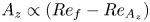 $A_z\propto (Re_f-Re_{A_z})$. The cross-over Reynolds numbers
  $Re_{A_z}$ obtained from this linear extrapolation are listed in table 2 for different noise levels (uncertainty is obtained using the bootstrap method). All these cross-overs
  $Re_{A_z}$ are consistent with the
  $Re_{A_z}=688\pm 10$ obtained by fitting
  $A_z$ using data taken over the range of noise levels.
Table 2. List of cross-over Reynolds numbers  $Re_{A_z}$ and
  $Re_{a_z}$ obtained from the linear extrapolation of decay rates and decay slopes as a function of
  $Re_f$ at different noise levels.
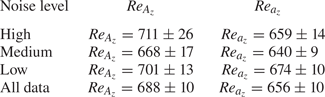
In contrast to the exponential decay of  $E_z$, the spanwise turbulent fraction evolution
  $F_z$ has a linear decay after the quench. Similarly, the second decay stage of
  $F_x$ is also linear for
  $Re_f\leq 425$ (see figure 4
 $a$ in § 3). The linear decays are fitted by the function
  $F_{i} = a_{i}t+b$ (
 $i=x,z$). The decay slopes
  $a_x$ and
  $a_z$ plotted as a function of
  $Re_f$ are shown in figure 15, respectively. The slope
  $a_x$ is always greater than
  $a_z$ in the range of
  $Re_f\in [300,425]$ irrespective of the noise level. This means there is a faster decay along the spanwise direction. This finding is consistent with the observation that the second decay stage of
  $F_x$ decays slower than the decay of
  $F_z$, as can be seen in figure 15. The slope
  $a_z$ scales linearly with
  $Re_f$ and is fitted by the function
 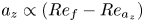 $a_z\propto (Re_f-Re_{a_z})$. The cross-overs
  $Re_{a_z}$ obtained from the linear fit with the data from different noise levels are listed in table 2. The cross-over
  $Re_{a_z}$ fitting
  $a_z$ for all the different noise levels is found at
  $Re_{a_z}=656\pm 10$, which is consistent with the value obtained from the fit of
  $a_z(Re_f)$ of each noise level.
Figure 15. Circles: slope  $a_{x}$ of the decay of the turbulent fraction
  $F_x$ after
  $\tau _z$ (
 $F_z$ has nearly decayed at
  $\tau _z$) as a function of
  $Re_f$; squares: slope
  $a_{z}$ of the decay of turbulent fraction
  $F_z$ as a function of
  $Re_f$; colour represents noise levels: red: high(
 $\sigma _A$); yellow: medium(
 $\sigma _B$); green: low(
 $\sigma _C$); blue: low(
 $\sigma _D$); purple dashed lines: linear fit of the mean decay slopes; error bar: standard deviation of
  $5$ realisations.
The cross-over Reynolds numbers obtained from the linear fit of  $A_z(Re_f)$ and
  $a_z(Re_f)$ are close to the self-sustained threshold. This threshold is at approximately
  $Re\approx 670$ (Klotz et al. Reference Klotz, Lemoult, Frontczak, Tuckerman and Wesfreid2017). The linear scalings are obtained far from the threshold, in the range
  $Re_f\in [300,525]$. This is different from many previous studies, which focused on the behaviour of characteristic times very close to the threshold (see for instance Bottin & Chaté Reference Bottin and Chaté1998; Shi et al. Reference Shi, Avila and Hof2013). An example of the investigation of
  $Re_f$ far from
  $Re_g$ is given in Schneider et al. (Reference Schneider, De Lillo, Buehrle, Eckhardt, Dörnemann, Dörnemann and Freisleben2010). They define a characteristic time from the lifetime distribution, using direct numerical simulations in the PCF geometry. The points in the range
  $Re_f\in [250,280]$, which is far from the
  $Re_g\approx 325$, are well fitted by a law
  $\tau ^{-1} \propto (Re_g-Re_f)$ (figure 3 of Schneider et al. Reference Schneider, De Lillo, Buehrle, Eckhardt, Dörnemann, Dörnemann and Freisleben2010). The linear scaling of characteristic times with
  $Re_f$ far from
  $Re_g$ provides an estimate of the value of the global stability threshold. In our case, we have also observed linear scalings of decay rates and slopes with
  $Re_f$. At present, we do not have a theoretical explanation for the linear scalings.
6. Conclusion
We have investigated the decay of turbulence in CPF using quench experiments. The final Reynolds number was varied over a wide range, and included all values where rapid decays are obtained. Thus we have extended the range of previous investigations which were primarily focused on values close to the critical point. We have provided experimental evidence for different decay rates for streaks and rolls during decay, which is consistent with previous theoretical work (Waleffe Reference Waleffe1997; Rolland Reference Rolland2018a). From the temporal evolution of the energy of streaks and rolls, we have shown that the rolls inject energy into the streaks through the lift-up mechanism during the first decay stage.
As in all plane channel experiments with moving walls, noise is generated in the reservoirs at the ends of the channel can induce turbulence in the flow. We have investigated the effects of this using multi-layer grids at the entrance (see figure 1) to reduce the noise. We find that the characteristic decay time and decay rates are independent of the noise levels. However, the permanent regime after the transient decay is sensitive to the noise intensities which are quantified by the susceptibility of the spanwise roll energy. The mean amplitude of the energy at a given  $Re_f$ increases with the noise which is a result of the advection of turbulent spots into the measurement field.
We have characterised the relaminarisation after a quench of an initially turbulent flow using the decay times, decay rates of the roll energy  $E_z$ and the decay slopes of the turbulent fraction of the roll component
  $F_z$. The comparison of decay times provides evidence that the rolls always decay faster than the streaks by a factor of approximately 2. The different decay rates are an essential feature in Walefffe's self-sustained model, which was first investigated in a minimal flow unit with periodic boundary conditions (Waleffe Reference Waleffe1997). Our experimental results support these ideas.
The decay of spanwise energy  $E_z$ displays an exponential tendency, reminiscent of a viscous damping. This feature has previously been highlighted in numerical quench studies in PCF by Rolland (Reference Rolland2015). The spanwise turbulent fraction
  $F_z$ displays a linear decay trend which has also been observed in numerical simulations of quench. The decay rates and decay slopes also contain a linear dependence on the
  $Re_f$, which is independent of the noise level. The theoretical explanation of this linear trend is not fully understood. The extrapolated value of
  $Re$ for which the decay rates and slopes vanish are close to the previously reported value for
  $Re_g\approx 670$ in CPF (Klotz et al. Reference Klotz, Lemoult, Frontczak, Tuckerman and Wesfreid2017).
The determination of the critical point  $Re_g$ in CPF using the crossing of the lifetime and splitting time has not been reported previously to our knowledge. However, it has been determined in PCF (Shi et al. Reference Shi, Avila and Hof2013), and in PPF (Gomé et al. Reference Gomé, Tuckerman and Barkley2020). It is thus very difficult to determine how close the extrapolated values obtained in our experiments are from
  $Re_g$. It is, however, noticeable that, using a fit at Reynolds numbers much smaller than the critical point, we can obtain a reasoned approximation.
The self-sustained process in channel flow is characterised by the presence of wavy streamwise streaks which lead to the breakdown of streaks and re-injection of energy into rolls due to nonlinear effects (Waleffe Reference Waleffe1997). In our measurements of the velocity field in § 3, we observed a fast extinction of the undulation of the streaks and the decay of the rolls followed by a slower decay of the straightened streaks. Our next step will be to measure the temporal evolution of the rolls and of the waviness of the streaks simultaneously. This is the subject of an ongoing investigation and it will allow us to investigate the interplay between the three components of the self-sustained process.
Supplementary movies
Supplementary movies are available at https://doi.org/10.1017/jfm.2021.89.
Acknowledgements
We gratefully acknowledge J. Rolland, Y. Duguet, R. Monchaux, S. Gomé, L. Tuckerman, D. Barkley, O. Dauchot and S. Bottin for fruitful discussions. We thank X. Benoit-Gonin, A. Fourgeaud, T. Darnige, O. Brouard and J. Laurent for technical help.
Funding
This work has benefited from the ANR TransFlow, and by starting grants obtained by B.S. from CNRS (INSIS) and ESPCI. T.M. was supported by a Joliot visiting professorship grant from ESPCI.
Declaration of interests
The authors report no conflict of interest.


 Open access