


1. Introduction
The motion of a rigid object in a fluid has been well studied during the last couple of centuries (Batchelor Reference Batchelor1967). In a bulk situation, for an incompressible Newtonian viscous fluid, the hydrodynamic force exerted on the object depends on its shape, size and speed, as well as on the fluid viscosity and frictional boundary conditions. Adding a neighbouring rigid wall to the latter problem was an obvious extension to consider, in view of the historical importance of lubricated contact mechanics in industry, but also because of the modern trends in miniaturization, colloidal surface science and confined biological physics. Such a modification introduces a symmetry breaking as well as different flow boundary conditions (Goldman, Cox & Brenner Reference Goldman, Cox and Brenner1967; O'Neill & Stewartson Reference O'Neill and Stewartson1967; Cooley & O'Neill Reference Cooley and O'Neill1969; Jeffrey & Onishi Reference Jeffrey and Onishi1981). A classical result from these studies shows that the force felt by a spherical particle approaching a no-slip wall increases inversely with the gap thickness, which implies no contact in finite time. Hocking (Reference Hocking1973) also explored the effect of slippage at the solid boundary, leading to a logarithmic factor and a contact in finite time. Happel & Brenner (Reference Happel and Brenner1983) provided a detailed account of this situation, including the related case of suspensions.
In view of the growing interest in soft matter towards complex materials, such as elastomers, gels or biological membranes, replacing the above rigid wall by an elastic boundary became of central importance. In such a context, the influence of the elastic response on the lubrication flow and associated forces and torques was addressed in both the normal (Balmforth, Cawthorn & Craster Reference Balmforth, Cawthorn and Craster2010; Leroy & Charlaix Reference Leroy and Charlaix2011; Leroy et al. Reference Leroy, Steinberger, Cottin-Bizonne, Restagno, Léger and Charlaix2012; Villey et al. Reference Villey, Martinot, Cottin-Bizonne, Phaner-Goutorbe, Léger, Restagno and Charlaix2013; Wang, Dhong & Frechette Reference Wang, Dhong and Frechette2015; Karan, Chakraborty & Chakraborty Reference Karan, Chakraborty and Chakraborty2018, Reference Karan, Chakraborty and Chakraborty2020, Reference Karan, Chakraborty and Chakraborty2021) and transverse (Sekimoto & Leibler Reference Sekimoto and Leibler1993; Beaucourt, Biben & Misbah Reference Beaucourt, Biben and Misbah2004; Skotheim & Mahadevan Reference Skotheim and Mahadevan2005; Weekley, Waters & Jensen Reference Weekley, Waters and Jensen2006; Urzay, Llewellyn Smith & Glover Reference Urzay, Llewellyn Smith and Glover2007; Snoeijer, Eggers & Venner Reference Snoeijer, Eggers and Venner2013; Bouchet et al. Reference Bouchet, Cazeneuve, Baghdadli, Luengo and Drummond2015; Salez & Mahadevan Reference Salez and Mahadevan2015; Saintyves et al. Reference Saintyves, Jules, Salez and Mahadevan2016; Davies et al. Reference Davies, Debarre, El Amri, Verdier, Richter and Bureau2018; Rallabandi et al. Reference Rallabandi, Oppenheimer, Zion and Stone2018; Vialar et al. Reference Vialar, Merzeau, Giasson and Drummond2019; Zhang et al. Reference Zhang, Bertin, Arshad, Raphael, Salez and Maali2020; Essink et al. Reference Essink, Pandey, Karpitschka, Venner and Snoeijer2021; Bertin et al. Reference Bertin, Amarouchene, Raphael and Salez2022; Bureau, Coupier & Salez Reference Bureau, Coupier and Salez2023) modes. This was achieved essentially by combining previous works on: (i) solid–solid contact and linear elasticity (Johnson Reference Johnson1985; Li & Chou Reference Li and Chou1997; Nogi & Kato Reference Nogi and Kato1997, Reference Nogi and Kato2002), and (ii) lubrication theory (Reynolds Reference Reynolds1886; Oron, Davis & Bankoff Reference Oron, Davis and Bankoff1997), resulting in the so-called soft-lubrication theory. These developments led in part to the design of non-invasive contactless mechanical probes for the rheology of soft, fragile and alive materials (Garcia et al. Reference Garcia, Barraud, Picard, Giraud, Charlaix and Cross2016; Basoli et al. Reference Basoli, Giannitelli, Gori, Mozetic, Bonfanti, Trombetta and Rainer2018). Further studies then incorporated elements of complexity in the substrate's response, through e.g. viscoelasticity (Pandey et al. Reference Pandey, Karpitschka, Venner and Snoeijer2016; Guan et al. Reference Guan, Barraud, Charlaix and Tong2017; Kargar-Estahbanati & Rallabandi Reference Kargar-Estahbanati and Rallabandi2021; Zhang et al. Reference Zhang, Arshad, Bertin, Almohamad, Raphaël, Salez and Maali2022) and poroelasticity (Kopecz-Muller et al. Reference Kopecz-Muller, Bertin, Raphaël, McGraw and Salez2023).
Interestingly, as materials get softer and increasingly liquid-like, solid capillarity takes the relay over bulk elasticity to eventually become the dominant restoring mechanism – a topic of recent and active research (Andreotti et al. Reference Andreotti, Baumchen, Boulogne, Daniels, Dufresne, Perrin, Salez, Snoeijer and Style2016). As a consequence, investigating soft-lubrication-like couplings in situations where the flow-induced interfacial deformation is resisted mainly by surface tension appears to be a relevant task. In a series of seminal articles, Lee, Leal and colleagues calculated the forces felt by a sphere moving close to a fluid interface in Stokes flow (Lee, Chadwick & Leal Reference Lee, Chadwick and Leal1979; Lee & Leal Reference Lee and Leal1980, Reference Lee and Leal1982; Berdan & Leal Reference Berdan II and Leal1982; Geller, Lee & Leal Reference Geller, Lee and Leal1986). Using Lorentz's reciprocal theorem, as well as a complete eigenfunction expansion in bipolar coordinates, they were able to exhibit the effects of the fluid interface – albeit in the regime where the gap between the sphere and the interface is large, and the interfacial deformation is negligible. It was found that the drag and torque acting on the sphere could be larger or smaller than their bulk counterparts, depending on the viscosities of the two layers. Related developments included the cases of slender objects (Yang & Leal Reference Yang and Leal1983), bubbles and droplets (Vakarelski et al. Reference Vakarelski, Manica, Tang, O'Shea, Stevens, Grieser, Dagastine and Chan2010; Chan, Klaseboer & Manica Reference Chan, Klaseboer and Manica2011), living microorganisms (Trouilloud et al. Reference Trouilloud, Tony, Hosoi and Lauga2008; Lopez & Lauga Reference Lopez and Lauga2014), slippery interfaces (Rinehart et al. Reference Rinehart, Lacis, Salez and Bagheri2020) and air–water interfaces with surface-active contaminants (Maali et al. Reference Maali, Boisgard, Chraibi, Zhang, Kellay and Würger2017; Bertin et al. Reference Bertin, Zhang, Boisgard, Grauby-Heywang, Raphaël, Salez and Maali2021).
While the above studies highlight clearly the richness and importance of motion near fluid interfaces, they focus on specific geometries and viscosity ratios. Hence the general capillary-lubrication regime has been scarcely explored so far. In the present paper, we thus investigate theoretically and numerically the lubrication flow and associated force generated by the prescribed normal motion of a rigid infinite cylinder near a deformable interface separating two immiscible and incompressible viscous fluids. We invoke a perturbative approach in dimensionless capillary compliance, and study the influence of the interfacial tension, viscosities of the fluids, and length scales of the problem on the resulting capillary-lubrication force.
The paper is organized as follows. We start by setting the general capillary-lubrication theoretical framework. Then the perturbation analysis is presented for the pressure and deformation fields up to first order in dimensionless capillary compliance, the latter being related directly to the capillary number. Finally, we discuss the results, compute quantitatively the capillary-lubrication force, and investigate the influence of all physical and geometrical parameters on the latter.
2. Capillary-lubrication theory
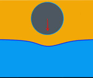
As shown in figure 1, we consider a rigid infinite cylinder of radius  $a$ moving in a fluid with a prescribed velocity normal to the nearby interface with a thin fluid film supported on a rigid substrate. The interface is characterized by its surface tension $\sigma$, and separates two incompressible Newtonian viscous liquids, with dynamic shear viscosities $\eta _1$ and $\eta _2$, as well as densities $\rho _1$ and $\rho _2=\rho _1-\delta \rho$ (with $\delta \rho >0$). The acceleration due to gravity is denoted $g$. The thickness profile $h_1(x,t)$ of the bottom liquid layer depends on the horizontal position $x$ as well as time $t$, and at large $x$, it equals the undeformed reference value $h_{b}$. The total thickness profile between the rigid substrate and the cylinder surface is denoted by $h_2(x,t)$. We also define the minimal distance $d(t)=h_2(0,t)-h_{b}$ between the undeformed fluid interface and the cylinder surface, the time derivative $\dot {d}(t)$ of which being the prescribed time-dependent velocity of the cylinder along $z$.
$z$.

Figure 1. Schematic of the system. A rigid infinite cylinder moves with a prescribed velocity normal to a nearby capillary interface between two incompressible Newtonian viscous liquids. The ensemble is placed atop a rigid substrate. The origin of spatial coordinates is located at the interface between the rigid substrate and the bottom liquid layer ( $z=0$) under the centre of mass of the cylinder ( $x=0$).
2.1. Governing equations
We neglect fluid inertia and assume the typical thicknesses, e.g.  $h_1(0,t)$ and $h_2(0,t)-h_1(0,t)$, of the two relevant liquid films of the problem to be much smaller than the proper horizontal length scale – whether the latter is the cylinder radius $a$, the capillary length $\sqrt {\sigma /(g\delta \rho )}$, or the hydrodynamic radius $\sqrt {2ad}$ (Leroy & Charlaix Reference Leroy and Charlaix2011), as discussed below. Therefore, we can invoke the lubrication theory (Reynolds Reference Reynolds1886; Oron et al. Reference Oron, Davis and Bankoff1997). Introducing the excess pressure fields $p_i(x,z,t)$ with respect to the hydrostatic contributions, and the horizontal velocity fields $u_i(x,z,t)$, in the two liquids indexed by $i=1,2$, the incompressible Stokes equations thus read, within the classical lubrication limit,
 $$\begin{gather} \frac{\partial p_i}{\partial z} = 0, \end{gather}$$
 $$\begin{gather}\frac{\partial p_i}{\partial x} = \eta_i\,\frac{\partial^2 u_i}{\partial z^2}. \end{gather}$$
Also, since typically the dominant flow is located only in the lubricated-contact region underneath the cylinder, we approximate the shape of the cylindrical surface by its parabolic expansion, leading to
 \begin{equation} h_2(x,t) \simeq h_{b}+d(t)+\frac{x^{2}}{2 a}.\end{equation}
 Finally, we close the set of equations by setting the flow boundary conditions. We impose no-slip at the three interfaces, as well as tangential and normal stress balances at the fluid interface. Hence at  $z = 0$ one has
 \begin{equation} u_{1} = 0, \end{equation}
while at  $z = h_1$ one has (Leal Reference Leal2007)
 $$\begin{gather} u_{2} = u_1, \end{gather}$$
 $$\begin{gather}\eta_2\,\frac{\partial u_2}{\partial z} = \eta_1\,\frac{\partial u_1}{\partial z}, \end{gather}$$
 $$\begin{gather}p_2-p_{1}\simeq\sigma\,\frac{\partial^2 h_1}{\partial x^2}+g(h_{{b}}-h_1)\,\delta\rho \end{gather}$$
(where the latter equation is valid under the small-slope approximation), and at  $z = h_2$ one has
 \begin{equation} u_{2} = 0. \end{equation}
Let us now non-dimensionalize the equations through
 \begin{equation} \left.\begin{gathered} h_1(x,t)= d^*\,H_1(X,T),\quad h_2(x,t)= d^*\,H_2(X,T),\quad x =lX, \\ z =d^*Z,\quad t = \frac{d^*}{c}\,T,\quad d(t) =d^*\,D(T), \\ u_1(x,z,t) =\frac{lc}{d^*}\,U_1(X,Z,T),\quad u_2(x,z,t) = \frac{lc}{d^*}\,U_2(X,Z,T),\\ p_1(x,t) =\frac{\eta_2c l^2}{d^{^*3}}\,P_1(X,T), \\ p_2(x,t)=\frac{\eta_2cl^2}{d^{^*3}}\,P_2(X,T),\quad h_{{b}} = d^*H_{b},\quad \dot {d}(t) =c\,\dot{D}(T), \end{gathered}\right\} \end{equation}
with the hydrodynamic radius  $l=\sqrt {2ad^*}$, and where $d^*$ and $c$ represent some characteristic vertical length and vertical velocity scales that can be set to e.g. $d(0)$ and $\dot {d}(0)$, respectively. Moreover, the viscosity ratio is denoted by $M = \eta _1/\eta _2$ and controls the effective slip length at the interface through (2.6). Specifically, an effective rigid-like no-slip condition (i.e. $u_2 = 0$) is obtained for $M\rightarrow \infty$, while an effective full-slip condition (i.e. infinite slip length) is obtained for $M\rightarrow 0$. Using these dimensionless variables, (2.3) becomes
 \begin{equation} H_2(X,T)=H_{b}+D(T)+X^{2}.\end{equation}
Solving (2.1) and (2.2) together with the boundary conditions (2.4)–(2.6) and (2.8) gives the velocity profiles
 \begin{align} U_{1} &={-}P_{2}^{\prime}\,\frac{(H_{2}-H_{1})^{2} Z}{2[H_{1}+M(H_{2}-H_{1})]} \nonumber\\ &\quad +P_{1}^{\prime}\left\{\frac{Z^{2}}{2 M}+\frac{Z}{H_{1}+M(H_{2}-H_{1})}\left[H_{1} (H_{1}-H_{2})-\frac{H_{1}^{2}}{2 M}\right]\right\}, \end{align}
 \begin{align} U_{2} &= P_{2}^{\prime}\left[\frac{Z^{2}-H_{2}^{2}}{2} -(Z-H_{2})\left\{H_{1}+\frac{M(H_{2}-H_{1})^{2}}{2 [H_{1}+M(H_{2}-H_{1})]}\right\}\right] \nonumber\\ &\quad +P_{1}^{\prime}\,\frac{(Z-H_{2})H_{1}^{2}}{2[H_{1}+M(H_{2}-H_{1})]}, \end{align}
where the prime symbol corresponds to the partial derivative with respect to  $X$. We then calculate the flow rates within the two liquid films as
 $$\begin{gather} Q_{1} =\int_{0}^{H_{1}} U_{1}\,\textrm{d} Z ={-}P_{2}^{\prime}\,\frac{H_{1}^{2}(H_{1}-H_{2})^{2}}{4[H_{1}+M (H_{2}-H_{1})]}-P_{1}^{\prime}\, \frac{H_{1}^{3}[H_{1}+4M(H_{2}-H_{1})]}{12 M[H_{1}+M(H_{2}-H_{1})]}, \end{gather}$$
 $$\begin{gather}Q_{2} =\int_{H_{1}}^{H_{2}} U_{2}\,\textrm{d} Z ={-}P_{2}^{\prime}\,\frac{(H_{2}-H_{1})^{3}}{12}\, \frac{4H_{1}+M(H_{2}-H_{1})}{H_{1}+M(H_{2}-H_{1})}-P_{1}^{\prime}\, \frac{H_{1}^{2}(H_{2}-H_{1})^{2}}{4[H_{1}+M(H_{2}-H_{1})]}. \end{gather}$$
Thanks to volume conservation, the flow rates allow us to write down the two thin-film equations, which read
 $$\begin{gather} \frac{\partial H_1}{\partial T}+Q_1^\prime = 0, \end{gather}$$
 $$\begin{gather}\frac{\partial (H_2-H_1)}{\partial T}+Q_2^\prime = 0. \end{gather}$$
Finally, (2.7) reads, in dimensionless form,
 \begin{equation} H_1^{\prime\prime}+{Bo}\,(H_{{b}}-H_1)=\kappa(P_2-P_1), \end{equation}
where  ${Bo} = (l/l_{{c}})^2$ denotes the Bond number of the problem, with $l_{{c}}=\sqrt {\sigma /(g\delta \rho )}$ the capillary length, and where $\kappa = {Ca}/\epsilon ^4$ is the dimensionless capillary compliance of the fluid interface, with ${Ca} = \eta _2c/\sigma$ a capillary number, and with $\epsilon =d^*/l$ and $\epsilon H_{{b}}$ the two small lubrication parameters of the problem.
Altogether, since  $H_2$ is known from (2.10) and the prescribed $D(T)$, there are actually three unknown fields in the problem: $H_1$, $P_1$ and $P_2$. These obey the set of three coupled differential equations given by (2.15)–(2.17), together with the symmetry conditions at $X = 0$
 \begin{equation} P_{i}^{\prime} = 0,\quad H_1^{\prime} = 0, \end{equation}
and the spatial boundary conditions at  $X\rightarrow \infty$
 \begin{equation} P_{i} \rightarrow 0,\quad H_1 \rightarrow H_{{b}}. \end{equation}
The whole study below is performed in terms of the dimensionless variables and dimensionless parameters provided above. We thus refer the reader to the present section for all the definitions.
3. Perturbation analysis
Following the approach of previous soft-lubrication studies (Sekimoto & Leibler Reference Sekimoto and Leibler1993; Skotheim & Mahadevan Reference Skotheim and Mahadevan2005; Urzay et al. Reference Urzay, Llewellyn Smith and Glover2007; Salez & Mahadevan Reference Salez and Mahadevan2015; Pandey et al. Reference Pandey, Karpitschka, Venner and Snoeijer2016), we assume that  $\kappa \ll 1$ and perform an expansion of the fields up to first order in $\kappa$, as
 $$\begin{gather} H_1 = H_{{b}} + \kappa \varDelta+O(\kappa^2), \end{gather}$$
 $$\begin{gather}P_1 =P_{10}+\kappa P_{11}+O(\kappa^2), \end{gather}$$
 $$\begin{gather}P_2 =P_{20}+\kappa P_{21}+O(\kappa^2), \end{gather}$$
where  $\kappa \varDelta$ is the deformation profile of the fluid interface at first order in $\kappa$, and $\kappa ^{j}P_{ij}$ is the excess pressure contribution of layer $i$ at perturbation order $j$. We further impose the following symmetry and spatial boundary conditions (see (2.18a,b) and (2.19a,b)): $P_{ij}^{\prime } = 0$ and $\varDelta ^{\prime } = 0$ at $X = 0$, as well as $P_{ij} \rightarrow 0$ and $\varDelta \rightarrow 0$ at $X\rightarrow \infty$.
3.1. Zeroth-order solution
At zeroth order in  $\kappa$, the fluid interface is undeformed, and the bottom-film thickness profile is constant and equal to $H_{{b}}$. Equations (2.15) and (2.16) can then be solved analytically using the symmetry and boundary conditions on the pressure fields. This leads to
 $$\begin{gather} P_{10} = \frac{9M\dot{D}}{2H_{{b}}^2}\ln\left(1+\frac{1}{\xi}\right), \end{gather}$$
 $$\begin{gather}P_{20} = \frac{9M^2\dot{D}}{2H_{{b}}^2}\left[\ln\left(1+\frac{1}{\xi}\right)- \frac{1}{\xi}-\frac{1}{6\xi^2}\right], \end{gather}$$
where we have introduced the auxiliary variable  $\xi (X,T) = M[D(T)+X^2]/H_{{b}}$. Interestingly, the zeroth-order excess pressure fields contain logarithmic terms, which differ notably from the rigid-substrate case where the excess pressure reads ${P_{{s}}=-3\dot {D}/(D+X^2)^2}$ (Jeffrey & Onishi Reference Jeffrey and Onishi1981). Nevertheless, the logarithmic terms decay algebraically in the far field, as ${\sim }1/X^2$, and the far-field expansion of the zeroth-order pressure field in the top layer reaches the solution for the no-slip rigid case, i.e. $P_{{20}} \simeq P_{s}$ at large $X$.
$X$.
3.2. First-order solution
At first order in  $\kappa$, (2.17) reads
 \begin{equation} \varDelta^{\prime\prime}-{Bo}\,\varDelta = P_{20}-P_{10} . \end{equation}
The formal solution of (3.6), satisfying the above symmetry (see (2.18a,b)) and boundary (see (2.19a,b)) conditions, is
 \begin{equation} \varDelta = \varDelta_{{c}}\cosh(X\sqrt{{Bo}})- \frac{1}{\sqrt{{Bo}}}\int_0^X\textrm{d}y\, [P_{20}(y)-P_{10}(y)]\sinh[(y-X)\sqrt{{Bo}}], \end{equation}
where  $\varDelta _{{c}}=\varDelta (X=0,T)=(1/\sqrt {{Bo}})\int _0^{\infty }\textrm {d}y\, [P_{10}(y)-P_{20}(y)]\exp (-y\sqrt {{Bo}})$ is the central deformation of the fluid interface. This solution can be evaluated numerically for fixed parameters $Bo$,
$Bo$,  $M$ and $H_{{b}}$, and a prescribed $D(T)$ trajectory.
In order to rationalize the asymptotic behaviours of the numerical solution, and to evaluate the central deformation, we employ an asymptotic-matching method, which is a usual approach for capillary problems (James Reference James1974; Lo Reference Lo1983; Dupré de Baubigny et al. Reference Dupré de Baubigny, Benzaquen, Fabié, Delmas, Aimé, Legros and Ondarçuhu2015). To do so, we assume a scale separation between: (i) an inner problem characterized by the horizontal length scale  $l$, where the dominant lubrication flow is located, and where gravity is absent; and (ii) an outer problem characterized by the capillary length $l_{{c}}$, where gravity regularizes the deformation. Specifically, we assume that $l\ll l_{{c}}$, i.e. ${Bo}\ll 1$. Let us first study the inner problem and associated inner solution $\varDelta _{{in}}(X,T)$. In the inner region, where $X\ll 1/\sqrt {{Bo}}$, (3.6) can be approximated by
 \begin{equation} \varDelta_{{in}}^{\prime\prime} = P_{20}-P_{10}. \end{equation}
The solution of this equation, satisfying the symmetry condition  $\varDelta _{{in}}'(X=0,T)=0$, reads
 \begin{align} \varDelta_{{in}} &= \mathcal{A}+\frac{9 \dot{D}}{4 H_{b}^{2}} \left\{(M-1)MX^2 \ln\left[1+\frac{H_{b}}{M(D+X^2)}\right]\right. \nonumber\\ &\quad +(1-M)(H_{b}+MD)\ln[H_{b}+M(D+X^2)]+[H_{{b}}+(M-1) D]M \ln (D+X^{2}) \nonumber\\ &\quad +4 \sqrt{D}\,M(1-M) X \tan ^{{-}1}\left(\frac{X}{\sqrt{D}}\right) +4 M(M-1)X \sqrt{D+\frac{H_{b}}{M}} \tan ^{{-}1}\left(\frac{X}{\sqrt{D+\dfrac{H_{b}}{M}}}\right) \nonumber\\ &\quad \left.{}-\frac{2M H_{b} X}{\sqrt{D}} \tan ^{{-}1}\left(\frac{X}{\sqrt{D}}\right)- \frac{H_{b}^{2}}{6 D^{3 /2}}\,X \tan ^{{-}1}\left(\frac{X}{\sqrt{D}}\right)\right\}, \end{align}
where  $\mathcal {A}$ is a function of $T$ only. The far-field behaviour of this inner solution reads
 \begin{align} \varDelta_{{in}} &\sim \mathcal{A} +\frac{9 \dot D}{4 H_{b}^{2}} \left\{ 2H_{b} \ln (X)+{\rm \pi} X \left[2 M(1-M) \sqrt{D}+2 M(M-1) \sqrt{D+\frac{H_{b}}{M}} \right.\right. \nonumber\\ &\quad \left.\left.{}-\frac{M H_{b}}{D^{1/2}}-\frac{H_{b}^{2}}{12D^{3 / 2}}\right] + \left[H_{b}(3-M)+(H_{b}+MD)(1-M)\ln(M)+\frac{H_{b}^{2}}{6 D} \right]\right\}. \end{align}
 Let us now study the outer problem and associated outer solution  $\varDelta _{{out}}(X,T)$. For $X$ large enough, (3.6) can be approximated by
 \begin{equation} \varDelta_{{out}}^{\prime\prime}-{Bo}\,\varDelta_{{out}} ={-}\frac{9\dot{D}}{2H_{{b}}X^2}. \end{equation}
We stress that it is essential here to keep a non-zero right-hand-side source term in the equation, in order to generate a logarithmic contribution as in the inner case. The solution of this equation, satisfying the boundary condition  $\varDelta _{{out}}\rightarrow 0$ at $X\rightarrow \infty$, reads
 \begin{align} \varDelta_{{out}} =\mathcal{B}\,\textrm{e}^{{-}X\sqrt{{Bo}}}+\frac{9\dot{D}}{4H_{{b}}} \left(\exp({-X\sqrt{{Bo}}})\int_{-\infty}^{X\sqrt{{Bo}}} \frac{\textrm{e}^t}{t}\,\textrm{d}t-\exp({X\sqrt{{Bo}}}) \int_{X\sqrt{{Bo}} }^{\infty}\frac{\textrm{e}^{{-}t}}{t}\,\textrm{d}t\right), \end{align}
where  $\mathcal {B}$ is a function of $T$ only. The small- $X$ behaviour of this inner solution reads
 \begin{equation} \varDelta_{{out}} \sim \mathcal{B}(1-X\sqrt{{Bo}})+\frac{9\dot{D}}{2H_{{b}}} \left[\gamma+\frac{1}{2}\ln({Bo})+\ln(X)\right], \end{equation}
where  $\gamma$ is the Euler constant.
Matching (3.13) and (3.10) allows us to determine the two unknown functions as
 \begin{align} \mathcal{A} &= \mathcal{B}+\frac{9 \dot D}{4 H_{{b}}^{2}}\left[H_{{b}}(M-3)+(H_{{b}} +MD) (M-1) \ln(M)-\frac{H_{{b}}^{2}}{6 D} \right] \nonumber\\ &\quad +\frac{9 \dot D\gamma}{2 H_{{b}}}+ \frac{9 \dot D}{4H_{{b}}}\ln({Bo}), \end{align}
 \begin{align} \mathcal{B} &= \frac{9 \dot{D} {\rm \pi}}{4 H_{{b}}^{2}\sqrt{{Bo}}} \left[2 M(M-1) \sqrt{D} +2 M(1-M) \sqrt{D+\frac{H_{{b}}}{M}}+\frac{M H_{{b}}}{\sqrt{D}}+\frac{H_{{b}}^{2}}{12D^{3 / 2}}\right]. \end{align}
In addition, using these matching conditions, the central deformation of the fluid interface can be evaluated from  $\varDelta _{{in}}(X=0,T)$, if ${Bo}\ll 1$, as
 \begin{align} \varDelta_{{c}}=\mathcal{A}+\frac{9 \dot{D}}{4 H_{b}^{2}}\,\{(1-M)(H_{b}+MD)\ln(H_{b}+MD) + [H_{{b}}+(M-1) D]M \ln (D)\}. \end{align}
 Finally, using (3.4), (3.5) and (3.7), as well as the above symmetry (2.18a,b) and boundary conditions (2.19a,b), we can solve (2.15) and (2.16) numerically at first order in  $\kappa$, and hence compute the first-order pressure fields. The derivation of these equations and the method for solving them are summarized in Appendix A. The results are discussed below.
4. Discussion
Hereafter, keeping  ${Bo}\ll 1$, we discuss the zeroth-order and first-order solutions, and investigate the influence of the two key parameters: the viscosity ratio $M$, and the thickness ratio $H_{{b}}$.
4.1. Zeroth-order pressure
In figure 2, we plot the zeroth-order excess pressure fields. For comparison, we also show the rigid-case excess pressure  $P_{{s}}=-3\dot {D}/(D+X^2)^2$ (Jeffrey & Onishi Reference Jeffrey and Onishi1981). As we can see, the pressure fields have opposite signs in the two layers. Moreover, the pressure in the top layer is reduced in the case of an undeformable fluid interface, as compared to the no-slip rigid case. This is due to the fact that horizontal motion at the fluid interface is possible in the former case, which reduces the velocity gradients and stresses. Also, we stress that despite their logarithmic forms in (3.4) and (3.5), the zeroth-order pressure fields in both layers decay algebraically towards zero at large $X$.
$X$.

Figure 2. (a) Zeroth-order excess pressure fields  $P_{i0}$, normalized by the cylinder's vertical velocity $\dot {D}$, as functions of horizontal coordinate $X$, as evaluated from (3.4) and (3.5) with $D = 1$, $M = 1.5$ and $H_{{b}} = 15$. (b) Zeroth-order excess pressure jump ${\rm \Delta} P_0 = P_{20}-P_{10}$ as a function of horizontal coordinate $X$, as obtained from (a). For comparison, we also show the rigid-case excess pressure $P_{{s}}=-3\dot {D}/(D+X^2)^2$ (Jeffrey & Onishi Reference Jeffrey and Onishi1981).
Let us now investigate the role of the viscosity ratio  $M$. The results are shown in figure 3. Increasing $M$, i.e. increasing the viscosity of the bottom liquid layer as compared to the top one, increases the pressure in both layers. This is expected, since increasing the viscosity ratio makes it harder to generate a flow within the bottom layer, which then gets closer to a rigid wall. This is supported by the curves in figure 3(b) and by (3.5), where, at high values of $M$,
$M$,  $P_{20}$ saturates to $P_{s}$. An interesting point to note in figure 3(a) and (3.4) is that the excess pressure in the bottom layer increases with $M$ as well, but saturates to $9\dot {D}/[2H_{{b}}(D+X^2)]$ at large $M$, which is dependent on the bottom layer thickness $H_{{b}}$. On the other hand, if $M$ is decreased towards zero, then (3.4) predicts that the excess pressure in the bottom layer vanishes completely. Besides, if $M$ is decreased towards zero, then (3.5) predicts that the excess pressure in the top layer saturates to a quarter of the no-slip rigid-wall value, which is the result expected for an effective full-slip interface (i.e. with infinite slip length). The pressure in the top layer is thus bounded at both extremes in $M$.
$M$.

Figure 3. Zeroth-order excess pressure fields (a)  $P_{10}$ and (b) $P_{20}$, normalized by the cylinder's vertical velocity $\dot {D}$, as functions of horizontal coordinate $X$, as evaluated from (3.4) and (3.5) with $D = 1$, $H_{{b}} = 15$ and various $M$ as indicated in the legends. For comparison, we also show the no-slip rigid-case excess pressure ${P_{{s}}=-3\dot {D}/(D+X^2)^2}$ (Jeffrey & Onishi Reference Jeffrey and Onishi1981), and its analogue for a full-slip rigid substrate, i.e. $P_{{s}}/4$.
The other important parameter to scan and study is the dimensionless bottom-layer thickness  $H_{b}$. Results are shown in figure 4. Increasing $H_{b}$ reduces the excess pressure fields in both layers. The two limiting behaviours for $P_{20}$ are the same as when varying $M$, as expected from (3.4) and (3.5), where it can be seen that the parameter $M/H_{b}$ is the relevant one.

Figure 4. Zeroth-order excess pressure fields (a)  $P_{10}$ and (b) $P_{20}$, normalized by the cylinder's vertical velocity $\dot {D}$, as functions of horizontal coordinate $X$, as evaluated from (3.4) and (3.5) with $D = 1$, $M = 1.5$ and various $H_{{b}}$ as indicated in the legends. For comparison, we also show the no-slip rigid-case excess pressure ${P_{{s}}=-3\dot {D}/(D+X^2)^2}$ (Jeffrey & Onishi Reference Jeffrey and Onishi1981), and its analogue for a full-slip rigid substrate, i.e. $P_{{s}}/4$.
4.2. Interface deflection
The first-order interface deflection is evaluated numerically from (3.7) and plotted in figure 5, along with the matched inner and outer solutions, given by (3.9) and (3.12). It is important to note here that the dimensionless slope is  $\epsilon \kappa \varDelta ^{\prime }$, and not only $\varDelta ^{\prime }$. Therefore, although the values of $\varDelta ^{\prime }$ may seem large, in the small dimensionless capillary compliance ( $\kappa \ll 1$) and lubrication ( $\epsilon \ll 1$) limits at stake in our study, the actual slope can still remain small. There is good agreement between the outer and general solutions, except in close proximity to the origin where the outer solution diverges logarithmically. In contrast, while unbounded in the far field, the inner solution agrees well with the general one near the origin.

Figure 5. Normalized first-order interface deflection  $\varDelta$ as a function of horizontal coordinate $X$ (black line), as calculated from (3.7), for $M = 1.5$, $H_{b} = 15$, ${Bo} = 0.01$, $D = 1$ and $\dot {D} = -1$ (i.e. the cylinder approaching the interface). For comparison, the matched inner (blue) and outer (red) solutions, given by (3.9) and (3.12), respectively, are shown. The inset shows a zoom of the small- $X$ region.
Let us now investigate the effects of viscosity ratio  $M$ and dimensionless bottom-layer thickness $H_{b}$ on the interface deflection. The results are shown in figure 6. We observe that the interface deflection increases with increasing $M$ or decreasing $H_{b}$. As discussed in the previous subsection, for vanishing $M$ or infinite $H_{b}$, the zeroth-order top-layer pressure $P_{20}$ reaches $P_{{s}}/4$, while the zeroth-order bottom-layer pressure $P_{10}$ vanishes, which leads to the minimal deflection profile. In contrast, as $M$ goes to infinity, $P_{20}$ reaches $P_{{s}}$, while $P_{10}$ increases to a function depending upon $H_{{b}}$. Thus the deflection saturates to an $H_{{b}}$-dependent profile. However, we stress that decreasing $H_{{b}}$ increases the deflection without any limit, as the zeroth-order pressure in the bottom layer does not have an upper bound in this case. In reality, such diverging pressure and thus interface deflection would require the consideration of higher-order, nonlinear effects in dimensionless capillary compliance.

Figure 6. (a) Normalized first-order interface deflection  $\varDelta$ as a function of horizontal coordinate $X$, as calculated from (3.7), for $H_{b} = 15$, ${Bo} = 0.01$, $D = 1$, $\dot {D} = -1$ (i.e. the cylinder approaching the interface), and various $M$ as indicated. (b) Same as (a) for $M=1.5$ and various $H_{b}$ as indicated.
4.3. First-order pressure
Integrating (2.15) and (2.16) numerically at first order in  $\kappa$ allows us to find the first-order pressure correction. Note that we consider only the first-order top-layer pressure $\kappa P_{21}$, for two reasons. First, this contribution is the only one required to eventually compute the first-order force exerted on the cylinder (see next subsection). Second, the first-order bottom-layer pressure decays slowly in $X$, and seems to depend on the size of the numerical window, indicating the potential need for a far-field regularization. Besides, we decompose $P_{21}$ into two contributions: (i) a dynamic adhesive-like term ${}_{\dot {D}^2} P_{21}$, depending on the square of the vertical velocity of the cylinder, which tends to attract the moving object towards the deformable interface (Kaveh et al. Reference Kaveh, Ally, Kappl and Butt2014; Salez & Mahadevan Reference Salez and Mahadevan2015; Wang et al. Reference Wang, Dhong and Frechette2015; Bertin et al. Reference Bertin, Amarouchene, Raphael and Salez2022); and (ii) an inertia-like term ${}_{\ddot {D}} P_{21}$, depending on the vertical acceleration of the cylinder, which is present here as a consequence of volume conservation (Salez & Mahadevan Reference Salez and Mahadevan2015; Bertin et al. Reference Bertin, Amarouchene, Raphael and Salez2022), even though the governing equations are free of inertia. The results are shown in figures 7, 8 and 9. We see that both pressure contributions are maximal at the centre ( $X=0$) and vanish quickly above $X\sim 1$. Besides, changing the viscosity ratio $M$ and the dimensionless bottom-layer thickness $H_{{b}}$ have the same effects as for the zeroth-order case.

Figure 7. Dynamic adhesive-like (blue) and inertia-like (red) contributions of the first-order pressure correction  $P_{21}$ in the top layer as a function of the horizontal coordinate $X$, obtained from numerical integration of (2.15) and (2.16), for $M = 1.5$, $H_{b} = 15$, ${Bo} = 0.01$, $D = 1$, $\dot {D} = -1$ and $\ddot {D} = 1$.

Figure 8. (a) Dynamic adhesive-like contribution  ${}_{\dot {D}^2} P_{21}$ of the first-order pressure correction in the top layer as a function of the horizontal coordinate $X$, obtained from numerical integration of (2.15) and (2.16), for $H_{b} = 15$, ${Bo} = 0.01$, $D = 1$, $\dot {D} = -1$, and various $M$ as indicated. (b) Same as (a) for $M=1.5$ and various $H_{b}$ as indicated.

Figure 9. (a) Inertia-like contribution  ${}_{\ddot {D}} P_{21}$ of the first-order pressure correction in the top layer as a function of the horizontal coordinate $X$, obtained from numerical integration of (2.15) and (2.16), for $H_{b} = 15$, ${Bo} = 0.01$, $D = 1$, $\dot {D} = -1$, $\ddot {D} = 1$, and various $M$ as indicated. (b) Same as (a) for $M=1.5$ and various $H_{b}$ as indicated.
4.4. Capillary-lubrication force
Since viscous stresses are negligible as compared to the excess pressure field within the lubrication framework, and since typically the excess pressure field obtained above vanishes beyond  $X\sim 1$ in the top layer, the normal capillary-lubrication force per unit length felt by the cylinder can be evaluated simply by integrating the excess pressure field in the top layer along the horizontal coordinate. Putting back dimensions, the force per unit length thus reads at first order in capillary compliance:
 \begin{align} F &= \int_{-\infty}^{+\infty}\textrm{d}\kern0.7pt x\, p_2 \simeq{-}\eta_2\dot {d}\left(\frac{a}{d}\right)^{3/2}\phi_0\left(\frac{MD}{H_{{b}}}\right) \nonumber\\ &\quad -\frac{\eta_2^{2}\dot {d}^2}{\sigma}\left(\frac{a}{d}\right)^{7/2}{}_{\dot{D}^2} \phi_1(M,H_{{b}},{Bo},D) \nonumber\\ &\quad +\frac{\eta_2^{2}\ddot{d}a}{\sigma} \left(\frac{a}{d}\right)^{5/2}{}_{\ddot{D}}\phi_1(M,H_{{b}},{Bo},D), \end{align}
where  $\phi _0$, ${}_{\dot {D}^2}\phi _1$ and ${}_{\ddot {D}}\phi _1$ are auxiliary functions depending on the parameters of the problem, $M$,
$M$,  $H_{{b}}$, as well as ${Bo}$, and importantly, potentially having extra dependencies in $d$ through $D$.
$D$.
Let us first study the zeroth-order contribution to the force, through the auxiliary function  $\phi _0$. By integrating (3.5), one can calculate $\phi _0$ and show that it depends only on the variable $MD/H_{{b}}$. The function is shown in figure 10. It is always positive, indicating a Stokes-like drag effect. At infinite $MD/H_{{b}}$, one recovers the no-slip rigid case (Jeffrey & Onishi Reference Jeffrey and Onishi1981), and the scaling of the force with $d$ is thus ${\sim }d^{-3/2}$. At vanishing $MD/H_{{b}}$, $\phi _0$ saturates to a quarter of the no-slip rigid value, which corresponds to the case of a full-slip rigid wall, with pressure $P_{{s}}/4$ as discussed above, and the scaling is once again ${\sim }d^{-3/2}$. In between these limits, we observe a smooth crossover and there is thus no clear power law in $d$.
$d$.

Figure 10. Zeroth-order auxiliary function  $\phi _0$ of the normal force (see (4.1)) obtained by integrating (3.5), and normalized by the corresponding value $3\sqrt {2}{\rm \pi}$ of the no-slip rigid case (Jeffrey & Onishi Reference Jeffrey and Onishi1981), as a function of the single rescaled variable $MD/H_{b}$. The dashed line shows a constant value $1/4$.
Then we study the first-order contributions to the force, through the two auxiliary functions  ${}_{\dot {D}^2}\phi _1$ and ${}_{\ddot {D}}\phi _1$. In these cases, there does not seem to be a simple combination of the parameters $M$,
$M$,  $H_{{b}}$, ${Bo}$ and variable $D$ that controls the auxiliary functions. These are evaluated numerically by integration of $P_{21}$, and plotted in figure 11 for various parameters. The two auxiliary functions are always positive and grow with increasing $M$ or decreasing $H_{{b}}$. They seem to saturate at either vanishing $M$ or infinite $H_{{b}}$. At infinite $M$, there might be a saturation as well. However, the functions seem unbounded when decreasing $H_{{b}}$. As a remark, the important increase observed for the auxiliary functions in some parametric ranges enforces stringent conditions on the dimensionless capillary compliance $\kappa$ so as to be in line with the perturbative approach.

Figure 11. First-order auxiliary functions (a)  ${}_{\dot {D}^2}\phi _1$ and (b) ${}_{\ddot {D}}\phi _1$ of the normal force (see (4.1)), as functions of the viscosity ratio $M$, as obtained from numerical integration of the first-order excess pressure $P_{21}$ in the top layer, for ${Bo}=0.01$, $D=1$, and various values of the dimensionless bottom-layer thickness $H_{{b}}$, as indicated. The lines are guides for the eye.
Finally, we wish to discuss briefly the corresponding three-dimensional problem of a sphere approaching the interface. In such a case, not only does the calculation procedure of the force and the deflection remain analogous to the current problem, but the dimensionless capillary compliance  $\kappa$ remains unchanged from the two-dimensional case, as the scales of the lubrication pressure and the Laplace pressure jump remain the same. Apart from modified numerical prefactors, the essential modification emerges in the scale of the forces, through a multiplication of the two-dimensional force per unit length by the relevant length scale in the third direction of space. This new length scale is the hydrodynamic radius, which implies that the zeroth-order force scales as ${\sim }\eta _2\dot {d}a^2/d$, and that the two components of the first-order force scale as ${\sim }\eta _2^{2}\dot {d}^2a^4/(\sigma d^3)$ and ${\sim }\eta _2^{2}\ddot{d}a^4/(\sigma d^2)$.
5. Conclusion
We have studied theoretically and numerically the capillary-lubrication force felt by an immersed infinite cylinder when approaching a thin viscous film supported on a rigid substrate. While the analogous scenario near an elastic wall has been studied extensively in recent years, our work investigated the influence of a fluid interface on such an emerging force by employing similar tools and a perturbation analysis in capillary compliance. In particular, we investigated the roles of two key dimensionless parameters: the viscosity ratio and the thickness ratio between the two layers.
As opposed to the case of a rigid wall, the zeroth-order (i.e. with no vertical deformation of the interface) pressure fields in both layers appeared to become logarithmic in space rather than rational functions, except in the far field, where asymptotic algebraic decays were recovered. Also, increasing the viscosity of the bottom layer, or reducing its thickness, led to a saturation towards the no-slip rigid-like behaviour. In contrast, a full-slip rigid behaviour was observed with the reduction of the bottom-layer viscosity, or the increase of the bottom-layer thickness. These zeroth-order pressure fields generate a long-range deflection of the interface, which was computed numerically along with an asymptotic study at small Bond numbers. Limiting behaviours of the interface deflection were observed with increasing or decreasing viscosity of the bottom layer, as well as increasing thickness. However, no limit was observed with the reduction of the bottom-layer thickness, and one thus expects nonlinearities to eventually regularize such a behaviour.
The first-order perturbations to the pressure fields due to the deformed interface were finally computed numerically, hence providing the correction to the Stokes drag felt by a particle due to the nearby deformable fluid interface. We identified two main dynamic contributions – (i) a velocity-dependent adhesive-like one, and (ii) an acceleration-dependent inertia-like one – and we used them to compute the total dimensionless force felt by the cylinder as it approaches the interface. The adhesive-like contribution essentially reduces the drag, while the inertia-like contribution increases it. The auxiliary functions that calculate the influence of viscosity and thickness ratios on the force were also evaluated and were seen to show limiting behaviours with increasing or decreasing bottom-layer viscosity and increasing bottom-layer thickness. Our results might find applications in confined colloidal and biophysical systems.
Funding
The authors thank V. Bertin, A. Carlson and C. Pedersen for interesting discussions. They acknowledge financial support from the European Union through the European Research Council under an EMetBrown (ERC-CoG-101039103) grant. Views and opinions expressed are, however, those of the authors only, and do not necessarily reflect those of the European Union or the European Research Council. Neither the European Union nor the granting authority can be held responsible for them. The authors also acknowledge financial support from the Agence Nationale de la Recherche under EMetBrown (ANR-21-ERCC-0010-01), Softer (ANR-21-CE06-0029) and Fricolas (ANR-21-CE06-0039) grants. Finally, they thank the Soft Matter Collaborative Research Unit, Frontier Research Center for Advanced Material and Life Science, Faculty of Advanced Life Science at Hokkaido University, Sapporo, Japan.
Declaration of interests
The authors report no conflict of interest.
Appendix A. First-order equations
The dimensionless fluxes in both layers can be written as
 $$\begin{gather} Q_1 = F_1(H_1,H_2)\,P_1^{\prime}+F_2(H_1,H_2)\,P_2^{\prime}, \end{gather}$$
 $$\begin{gather}Q_2 = F_3(H_1,H_2)\,P_1^{\prime}+F_4(H_1,H_2)\,P_2^{\prime}, \end{gather}$$
where the  $F_i$ are the auxiliary functions found in (2.13) and (2.14), which depend on $H_1$ and $H_2$. While $H_2 = D(T)+X^2$ is a function that is independent of the interface deflection, $H_1$ depends on the interface deflection and thus changes with the order of the equation. Taylor expansions of the auxiliary functions at first order in $\kappa$ give us
 \begin{equation} F_i(H_1,H_2) \simeq F_i(H_{b},H_2) + \kappa \varDelta \left.\frac{\partial F_i}{\partial H_1}\right\rvert_{H_1=H_{b}}+O(\kappa^2). \end{equation}
Since the auxiliary functions are known functions of  $H_1$, we can calculate easily their partial derivatives with respect to $H_1$, which are denoted by $G_i = {\partial F_i}/{\partial H_1}$. Hence the fluxes above can be approximated at first order in compliance, as
 \begin{align} Q_1 &\simeq [F_1(H_{b},H_2)\,P_{10}^{\prime}+\kappa(F_1(H_{b},H_2)\,P_{11}^{\prime}+{\rm \Delta} G_1(H_{b},H_2)\,P_{10}^{\prime})] \nonumber\\ &\quad +[F_2(H_{b},H_2)\,P_{20}^{\prime}+\kappa(F_2(H_{b},H_2)\,P_{21}^{\prime}+{\rm \Delta} G_2(H_{b},H_2)\,P_{20}^{\prime})]+O(\kappa^2), \end{align}
 \begin{align} Q_2 &\simeq [F_3(H_{b},H_2)\,P_{10}^{\prime}+\kappa(F_3(H_{b},H_2)\,P_{11}^{\prime}+ {\rm \Delta} G_3(H_{b},H_2)\,P_{10}^{\prime})] \nonumber\\ &\quad +[F_4(H_{b},H_2)\,P_{20}^{\prime}+\kappa(F_4(H_{b},H_2)\,P_{21}^{\prime}+{\rm \Delta} G_4(H_{b},H_2)\,P_{20}^{\prime})]+O(\kappa^2). \end{align}
The  $\kappa$-independent parts of these equations correspond to the fluxes at zeroth order, and can be used in conjunction with (2.15) and (2.16) in order to obtain the analytical expressions of the zeroth-order pressure fields (see (3.4) and (3.5)). Furthermore, the above fluxes can be combined in order to derive the thin-film equations at $O(\kappa )$, which read
 $$\begin{align}
\frac{\partial \varDelta}{\partial T} &={-}\frac{\partial}{\partial
X}[F_1(H_{b},H_2)\,P_{11}^{\prime}+ {\rm \Delta}
G_1(H_{b},H_2)\,P_{10}^{\prime}+F_2(H_{b},H_2)\,P_{21}^{\prime}\nonumber\\ &\quad +
{\rm \Delta} G_2(H_{b},H_2)\,P_{20}^{\prime}],
\end{align}$$
$$\begin{align}
\frac{\partial \varDelta}{\partial T} &={-}\frac{\partial}{\partial
X}[F_1(H_{b},H_2)\,P_{11}^{\prime}+ {\rm \Delta}
G_1(H_{b},H_2)\,P_{10}^{\prime}+F_2(H_{b},H_2)\,P_{21}^{\prime}\nonumber\\ &\quad +
{\rm \Delta} G_2(H_{b},H_2)\,P_{20}^{\prime}],
\end{align}$$ $$\begin{align}\frac{\partial \varDelta}{\partial T} &= \frac{\partial}{\partial X}[F_3(H_{b},H_2)\,P_{11}^{\prime}+{\rm \Delta} G_3(H_{b},H_2)\,P_{10}^{\prime}+F_4(H_{b},H_2)\,P_{21}^{\prime}+{\rm \Delta} G_4(H_{b},H_2)\,P_{20}^{\prime}]. \end{align}$$
These equations can be spatially integrated once, and rearranged to give
 $$\begin{gather} F_1(H_{b},H_2)\,P_{11}^{\prime}+F_2(H_{b},H_2)\,P_{21}^{\prime} ={-}\int_0^X\frac{\partial \varDelta}{\partial T}\,\textrm{d}\kern0.7pt X -\mathcal{J}_1, \end{gather}$$
 $$\begin{gather}F_3(H_{b},H_2)\,P_{11}^{\prime}+F_4(H_{b},H_2)\,P_{21}^{\prime} = \int_0^X\frac{\partial \varDelta}{\partial T}\,\textrm{d}\kern0.7pt X -\mathcal{J}_2, \end{gather}$$
where we have invoked two new auxiliary functions:
 $$\begin{gather} \mathcal{J}_1 = {\rm \Delta} G_1(H_{b},H_2)\,P_{10}^{\prime}+{\rm \Delta} G_2(H_{b},H_2)\,P_{20}^{\prime}, \end{gather}$$
 $$\begin{gather}\mathcal{J}_2 = {\rm \Delta} G_3(H_{b},H_2)\,P_{10}^{\prime}+{\rm \Delta} G_4(H_{b},H_2)\,P_{20}^{\prime}. \end{gather}$$
Then the derivatives of the first-order pressure fields read
 $$\begin{gather} P_{11}^{\prime}=\frac{F_4\mathcal{H}_1-F_2\mathcal{H}_2}{F_4F_1-F_2F_3}, \end{gather}$$
 $$\begin{gather}P_{21}^{\prime}={-}\frac{F_3\mathcal{H}_1-F_1\mathcal{H}_2}{F_4F_1-F_2F_3}, \end{gather}$$
where  $\mathcal {H}_1$ and $\mathcal {H}_2$ denote the right-hand sides of (A8) and (A9). The above expressions can be integrated over $X$, imposing the vanishing of the pressure in the far field, to give us the first-order pressure fields. We note that the above equations are linear combinations of $\mathcal {H}_1$ and $\mathcal {H}_2$. This property is exploited directly in order to calculate separately the components of the first-order pressure fields depending on the acceleration and the squared velocity. To this aim, we introduce two new auxiliary functions:
 $$\begin{gather} \mathcal{Q}_1 =\int_0^X\left.\frac{\partial \varDelta}{\partial T}\right\rvert_{\dot{D}^2}\textrm{d}\kern0.7pt X, \end{gather}$$
 $$\begin{gather}\mathcal{Q}_2 = \int_0^X\left.\frac{\partial \varDelta}{\partial T}\right\rvert_{\ddot{D}}\textrm{d}\kern0.7pt X, \end{gather}$$
that denote the integrals of the time derivatives of the deflection corresponding to the squared-velocity-dependant and acceleration-dependant components, respectively. These time derivatives are found by differentiating the pressure fields with respect to time, as
 $$\begin{gather} \frac{\partial P_{10}}{\partial T} = \frac{9M\ddot{D}}{2H_{{b}}^2} \ln\left(1+\frac{1}{\xi}\right)-\frac{9M^2\dot{D}^2}{2H_{{b}}^3}\,\frac{1}{\xi(\xi+1)}, \end{gather}$$
 $$\begin{gather}\frac{\partial P_{20}}{\partial T} = \frac{9M^2\ddot{D}}{2H_{{b}}^2}\left[\ln\left(1+\frac{1}{\xi}\right)-\frac{1}{\xi}- \frac{1}{6\xi^2}\right]+\frac{9M^3\dot{D}^2}{2H_{{b}}^3}\left[\frac{-1}{\xi(\xi+1)}+ \frac{1}{\xi^2}+\frac{1}{3\xi^3}\right], \end{gather}$$
and injecting the latter expressions inside the integral of (3.7). In the above expressions, we see that the first terms in the right-hand sides characterize the effects of acceleration of the cylinder, while the second terms characterize the effects of squared velocity. Then  $\mathcal {Q}_1$ and $\mathcal {Q}_2$ can be evaluated numerically. As opposed to $\mathcal {Q}_1$ and $\mathcal {Q}_2$, both $\mathcal {J}_1$ and $\mathcal {J}_2$ are independent of $\ddot {D}$ but are directly proportional to $\dot {D}^2$, since the deflection $\varDelta$ and zeroth-order pressure gradients $P_{10}^{\prime }$ and $P_{20}^{\prime }$ are proportional to $\dot {D}$. Using the above properties and expressions, we split $\mathcal {H}_1$ and $\mathcal {H}_2$ into acceleration-dependent and squared-velocity-dependent terms as
 $$\begin{gather} (\mathcal{H}_1)_{\dot{D}^2} ={-}\mathcal{Q}_1-\mathcal{J}_1, \end{gather}$$
 $$\begin{gather}(\mathcal{H}_2)_{\dot{D}^2} = \mathcal{Q}_1-\mathcal{J}_2, \end{gather}$$
 $$\begin{gather}(\mathcal{H}_1)_{\ddot{D}} ={-}\mathcal{Q}_2, \end{gather}$$
 $$\begin{gather}(\mathcal{H}_2)_{\ddot{D}} = \mathcal{Q}_2, \end{gather}$$
which are eventually used in (A12) and (A13) in order to calculate the corresponding contributions to the first-order pressure fields separately.


 Open access