


1. Introduction
Gravity currents are flows driven by density differences and occur ubiquitously in natural and man-made environments (Simpson Reference Simpson1997; Ungarish Reference Ungarish2009). For a long time, the lock-exchange set-up has served as a paradigm configuration for studying the propagation of gravity currents (Shin, Dalziel & Linden Reference Shin, Dalziel and Linden2004; Adduce, Sciortino & Proietti Reference Adduce, Sciortino and Proietti2012; La Rocca et al. Reference La Rocca, Adduce, Lombardi, Sciortino and Hinkermann2012a,Reference La Rocca, Adduce, Sciortino, Bateman and Bonifortib; Ottolenghi et al. Reference Ottolenghi, Adduce, Inghilesi, Armenio and Roman2016a). In the classic lock-exchange experiments, two fluids of different densities are separated by a removable lock gate in a long horizontal channel. The motion of the two fluids in the channel is initiated when the lock gate is removed. The gravity currents in the classic lock-exchange set-up are also called planar gravity currents as the flows are bounded in the spanwise direction by the channel walls.
Gravity currents may also be influenced by the presence of a sloping boundary. In the literature, a number of studies have investigated planar gravity currents propagating on a favourable slope (Beghin, Hopfinger & Britter Reference Beghin, Hopfinger and Britter1981; Bonnecaze & Lister Reference Bonnecaze and Lister1999; Pawlak & Armi Reference Pawlak and Armi2000; Rastello & Hopfinger Reference Rastello and Hopfinger2004; Maxworthy & Nokes Reference Maxworthy and Nokes2007; Maxworthy Reference Maxworthy2010; Dai Reference Dai2013a, Reference Dai2014, Reference Dai2015; Dai & Huang Reference Dai and Huang2016; Negretti, Flòr & Hopfinger Reference Negretti, Flòr and Hopfinger2017; Ottolenghi, Cenedese & Adduce Reference Ottolenghi, Cenedese and Adduce2017b; Steenhauer, Tokyay & Constantinescu Reference Steenhauer, Tokyay and Constantinescu2017), while some have investigated planar gravity currents propagating on an adverse slope (Jones et al. Reference Jones, Cenedese, Chassignet, Linden and Sutherland2014; Marleau, Flynn & Sutherland Reference Marleau, Flynn and Sutherland2014; Lombardi et al. Reference Lombardi, Adduce, Sciortino and La Rocca2015; Ottolenghi et al. Reference Ottolenghi, Adduce, Inghilesi, Roman and Armenio2016b, Reference Ottolenghi, Adduce, Roman and Armenio2017a). For the planar gravity currents propagating on a favourable slope, Beghin et al. (Reference Beghin, Hopfinger and Britter1981) observed that planar gravity currents may go through an acceleration phase followed by a deceleration phase, and developed the thermal theory to describe the two phases of motion. Dai (Reference Dai2013a, Reference Dai2014) further categorised the deceleration phase of the planar gravity currents propagating on a favourable slope into an early stage, where the buoyancy force is in balance with the inertia force, and a late stage, where the buoyancy force is in balance with the viscous force.
Compared with the planar gravity currents, the gravity currents propagating on a horizontal or sloping boundary without being bounded in the spanwise direction have received less attention (Cantero, Balachandar & Garcia Reference Cantero, Balachandar and Garcia2007; La Rocca et al. Reference La Rocca, Adduce, Sciortino and Pinzon2008; Sahuri et al. Reference Sahuri, Kaminski, Flynn and Ungarish2015; Dai & Wu Reference Dai and Wu2016; Inghilesi et al. Reference Inghilesi, Adduce, Lombardi, Roman and Armenio2018). However, this configuration is more similar to that of turbidity currents down a continental shelf and powder snow avalanches (Hopfinger Reference Hopfinger1983; Ouillon, Meiburg & Sutherland Reference Ouillon, Meiburg and Sutherland2019). The gravity currents propagating on unbounded uniform slopes may also go through an acceleration phase followed by a deceleration phase. Using the shallow water model, Webber, Jones & Martin (Reference Webber, Jones and Martin1993) and Tickle (Reference Tickle1996) predicted that the gravity currents on unbounded uniform slopes would take a self-similar circular wedge shape. Using laboratory experiments, Ross, Linden & Dalziel (Reference Ross, Linden and Dalziel2002) showed that the Boussinesq gravity currents on unbounded uniform slopes take a shape which is more akin to a triangular wedge. Using high-resolution direct numerical simulations, Zgheib, Ooi & Balachandar (Reference Zgheib, Ooi and Balachandar2016) confirmed the observations made by Ross et al. (Reference Ross, Linden and Dalziel2002) and reported that, for the Boussinesq gravity currents propagating on unbounded uniform slopes, the heavy fluid may initially propagate outward from the lock in a diverging manner but converge towards the centre of the gravity currents at a later time.
The Boussinesq gravity currents propagating on unbounded uniform slopes have recently been investigated by Dai & Huang (Reference Dai and Huang2020). It is reported that there are two stages of the deceleration phase for the Boussinesq gravity currents on unbounded uniform slopes and different power relationships apply in the early and late stages of the deceleration phase. This study is a continuation of the investigation on the Boussinesq gravity currents on unbounded uniform slopes conducted by the authors. Our focus is on the influence of the relative density difference on the deceleration phase of the propagation. The relative density difference between the heavy fluid and light ambient fluid  $\epsilon = (\rho _1-\rho _0)/\rho _0$ is varied in the range $0.05 \le \epsilon \le 0.15$ in this study, where $\rho _1$ and $\rho _0$ are the densities of the heavy and light ambient fluids, respectively. We may quantitatively measure the influence of the slope angle and the relative density difference on the propagation of gravity currents. As we will show, the non-Boussinesq gravity currents on the steeper unbounded uniform slopes in this study ( $12\,^\circ$, $9\,^\circ$ and $6\,^\circ$) may have become Boussinesq ones in the late deceleration phase while the non-Boussinesq gravity currents on the milder unbounded uniform slopes in this study ( $3\,^\circ$ and $0\,^\circ$) may remain non-Boussinesq ones in the late deceleration phase. In § 2, we summarise the theoretical relationships between the front location and time in the early stage and late stage of the deceleration phase. The experimental set-up is described in § 3. Qualitative and quantitative results are presented in § 4 and the conclusions are drawn in § 5.
2. Theoretical background
The configuration of the problem is sketched in figure 1. The density of the heavy fluid in the lock is  ${\rho }_1$ and the density of the light ambient fluid is ${\rho }_0$. The relative density difference is $\epsilon = (\rho _1-\rho _0)/\rho _0$ or equivalently we may define the density ratio between the ambient and heavy fluids as $\gamma =\rho _0/\rho _1$. The density ratio is related to the relative density difference via $\gamma = (1+\epsilon )^{-1}$. For the non-Boussinesq case, here we generalise the Boussinesq wedge integral model in Dai & Huang (Reference Dai and Huang2020) without invoking the Boussinesq approximation. In the wedge integral model, the width and height of the wedge are taken as $b= {\rm \pi}l$ and $h=l \tan \theta$, where $l$ represents the length of the wedge. The volume of the wedge is $V=S_3 l^3 \tan \theta$, where $S_3=1/3$ is a shape factor for a triangular wedge (Ross et al. Reference Ross, Linden and Dalziel2002).

Figure 1. Sketch of the experimental set-up. The uniform slope makes an angle  $\theta$ with the horizontal plane. Panel (a) shows the top view and panel (b) shows the side view of the tank. In panel (a), $l$ and $b$ represent the length and width of the self-similar wedge. In panel (b), $h$ represents the height of the wedge. The heavy fluid initially contained in the lock has density $\rho _1$ while the light ambient fluid has density $\rho _0$. The front location $x_f$ is measured from the lock gate and the virtual origin is at a distance $x_0$ upslope of the lock gate.
The convection of the gravity current is driven by the density difference between the heavy fluid in the current and the light ambient fluid in the environment. The influence of the drag force is relatively small compared with the influence of turbulent entrainment, as discussed by Dai (Reference Dai2013a,Reference Daib, Reference Dai2014). Therefore, the drag force is neglected in our wedge integral model for the non-Boussinesq case. Without the Boussinesq approximation, the linear momentum equation takes the form
 \begin{equation} \frac{\textrm{d} }{\textrm{d} t} ((\rho + \rho_0 C_A) V U) = \rho_0 B \sin \theta, \end{equation}
where  $\rho$ is the density of the heavy fluid in the current, $C_A$ is the ‘added mass’ coefficient, which takes into account the ambient fluid carried along with the gravity currents, $U$ is the velocity of the centre of mass of the current wedge, $B=V_0 g(\rho _1-\rho _0)/\rho _0$ is the buoyancy which is conserved during the propagation of gravity currents and $t$ is the time. The density of the heavy fluid in the current, $\rho$, is not a constant and will gradually decrease due to entrainment of light ambient fluid as the current propagates downslope. The added mass coefficients for a circular cylinder and a sphere are given as $1$ and $0.5$, respectively, by Batchelor (Reference Batchelor1967). For a streamlined wedge of width $b$ and length $l$, the added mass coefficient for the wedge is estimated as $C_A=0.5$ in this study (Korotkin Reference Korotkin2008).
With the assumption of turbulent entrainment (Ellison & Turner Reference Ellison and Turner1959), the mass conservation takes the form
 \begin{equation} \frac{\textrm{d} V }{\textrm{d} t} = \alpha U A_E, \end{equation}
where  $A_E=S_4 l^2 \tan \theta$ is the area over which the entrainment takes place, $S_4=2 \sqrt {2}$ is another shape factor (Ross et al. Reference Ross, Linden and Dalziel2002) and $\alpha$ is the entrainment coefficient. From (2.2) and using $U=\textrm {d}x/\textrm {d}t$, we may derive
 \begin{equation} l = \frac{S_4 \alpha}{3 S_3} x, \end{equation}
where  $x$ is the distance measured from the ‘virtual origin’ to the centre of mass of the wedge. By using $U=\textrm {d} x/\textrm {d}t$ and the chain rule $\textrm {d}/\textrm {d}t=U \textrm {d}/\textrm {d} x$ to solve (2.2), the independent variable in (2.2) is transformed from $t$ to $x$. The ‘virtual origin’ is located $x_0$ upslope of the lock gate and can be identified by extrapolating the width of the wedge in the upslope direction, as shown in figure 1. Upon substituting (2.3) into (2.1), we may derive the solution for the momentum equation, i.e.
 \begin{equation} U^2 = U_0^2 \frac{{(1+\varDelta)}^2}{{(X^3+\varDelta)}^2}+ U^2_\infty \frac{(X^4-1)+4 \varDelta (X-1)}{{(X^3+\varDelta)}^2}, \end{equation}
where  $U_0$ is the initial mass-centre velocity,
 \begin{equation} U^2_\infty = \frac{27 B S^2_3 \cos \theta}{2 x^2_0 \alpha^3 S^3_4 (1+C_A)} \quad \mbox{and} \quad \varDelta = \frac{1-\gamma}{\gamma} \frac{27 S^2_3 V_0}{x^3_0 \alpha^3 S^3_4 \tan \theta (1+C_A)} \end{equation}
and  $X=x/x_0$ is introduced for a clear and concise form of the solution (2.4).
Our wedge integral model predicts that, for gravity currents starting from a quiescent condition, the centre of mass velocity reaches its maximum at  $X=X_M$, which satisfies the following relationship
 \begin{equation} X_M^6+8 \varDelta X^3_M-3(4 \varDelta+1)X^2_M+2 \varDelta^2=0, \end{equation}
by setting the spatial derivative of (2.4) to zero. In the Boussinesq limit when  $\epsilon \rightarrow 0$ (i.e. $\gamma \rightarrow 1$ and $\varDelta \rightarrow 0$), we note that $X_M \rightarrow 3^{1/4}$ as previously shown by Dai & Huang (Reference Dai and Huang2020) in the Boussinesq case.
Since in the experiments the front location is more easily measurable than the centre of mass, we use the geometric relation for a triangular wedge  $(x_f + x_0) = {x} + l /2$, i.e. $(x_f + x_0)= ( 1 + S_4 \alpha /6 S_3 ) x$, to express the front location $x_f$ in place of the centre of mass location. Please note that the front location $x_f$ is measured from the lock gate and the distance from the virtual origin to the front is given by $(x_f+x_0)$. Consequently, the front velocity is related to the centre of mass velocity via $U_f = ( 1 + S_4 \alpha /6 S_3 ) U$ and the maximum front velocity ${U_{f}}_{max}$ can be expressed as
 \begin{equation} {U_{f}}_{max} = \left(1+\frac{S_4 \alpha}{6 S_3}\right) \sqrt{\frac{27 B S^2_3 \cos \theta}{2 x^2_0 \alpha^3 S^3_4 (1+C_A)}} \sqrt{\frac{{(X_M^4-1)+4 \varDelta(X_M-1)}}{{(X_M^3+\varDelta)}^2}}. \end{equation}
 For gravity currents sufficiently far into the deceleration phase such that  $X \gg 1$ and $X \gg 4 \varDelta$, the front velocity approaches the asymptote
 \begin{equation} U_f = \left(1+\frac{S_4 \alpha}{6 S_3}\right)^2 \sqrt{\frac{27 B S^2_3 \cos \theta}{2 \alpha^3 S^3_4 (1+C_A)}} {(x_f+x_0)}^{{-}1}. \end{equation}
The wedge integral model has been obtained with the hypothesis of non-trivial or moderate values of relative density difference and will be applied for relative density differences in the range  $0.05 \le \epsilon \le 0.15$. The application to cases with even larger relative density difference at $\epsilon > 0.15$ is not corroborated and is beyond the scope of the present work. Since $\varDelta \approx O(\epsilon )$, as we considered the relative density difference in the range $0.05 \le \epsilon \le 0.15$, the condition $X \gg 4 \varDelta$ is no more stringent than $X \gg 1$. Upon integration, (2.8) can be rewritten in the following form with an integration constant $t_{I}$
 \begin{equation} {(x_f+x_0)}^2 = {(K_I {B})}^{1/2} (t+t_{I}), \end{equation}
where
 \begin{equation} K_I = {\left( 1 + \frac{ S_4 \alpha}{6 S_3} \right)}^{4} \frac{{54} S^2_3 \cos \theta}{\alpha^{3} S^{3}_4 {(1+C_A)}}, \end{equation}
which is independent of  $B$ and is a function of the slope angle $\theta$. According to the Buckingham theorem, the dimensionless constant $K_I$ should be a function of the slope angle and the relative density difference. The dependence of the dimensionless constant $K_I$ on the relative density difference is not explicit in (2.10) but is implicit via the influence of the relative density difference on the entrainment coefficient $\alpha$. The density difference between the heavy fluid in the current and the light ambient fluid stabilises the interface and the entrainment coefficient is expected to decrease as the relative density difference increases (Ellison & Turner Reference Ellison and Turner1959; Hacker, Linden & Dalziel Reference Hacker, Linden and Dalziel1996; Hallworth et al. Reference Hallworth, Huppert, Phillips and Sparks1996; Johnson & Hogg Reference Johnson and Hogg2013).
From the scaling analysis, it has been shown that the relationship (2.9) is essentially a statement of balance between the buoyancy force and inertia force (Dai & Huang Reference Dai and Huang2020). In the Boussinesq case, the relative density difference does not play a role since  $\epsilon \rightarrow 0$ ( $\gamma \rightarrow 1$). In the non-Boussinesq case, the dimensionless constant $K_I$ is a function of both the slope angle and the relative density difference. In this study, we shall term the time period during which (2.9) applies the early stage of deceleration phase.
As will be shown later, for the gravity currents propagating on unbounded uniform slopes equal to or greater than  $6\,^\circ$, an ‘active’ head separates from the body of the current in the late deceleration phase. In the late deceleration phase, when the viscous force becomes more important, the viscous force per unit mass scales as $\nu (x_f+x_0) t^{-1} {\delta }^{-1} {V_0}^{-1/3}$, where the viscous stress per unit density is estimated as $\nu (x_f+x_0) {t}^{-1} {\delta }^{-1}$, the thickness of the boundary layer at the interface between the current and ambient fluid is estimated as $\delta \sim {(\nu t)}^{1/2}$ and ${V_0}^{1/3}$ is an estimate for the length scale for the ‘active’ current wedge (Dai & Huang Reference Dai and Huang2020). When a balance between the buoyancy force per unit mass, which scales as $B {(x_f+x_0)}^{-3}$, and the viscous force per unit mass, which scales as $\nu (x_f+x_0) t^{-1} {\delta }^{-1} {V_0}^{-1/3}$, is struck for the ‘active’ current head, the following relationship applies in the late deceleration phase, i.e.
 \begin{equation} {(x_f+x_0)}^{8/3} = K_{VS} {\left( \frac{{B}^{2} V^{2/3}_0 }{\nu} \right)}^{1/3} ({t+t_{VS}}), \end{equation}
where  $K_{VS}$ is an experimental constant and $t_{VS}$ the $t$ intercept.
For the gravity currents propagating on unbounded uniform slopes equal to or less than  $3\,^\circ$, the gravity currents maintain an integrated shape. In the early stage of deceleration phase, when the buoyancy and inertia forces are in balance, the front location history similarly follows the relationship (2.9). In the late stage of the deceleration phase, the gravity currents maintain an integrated shape and the viscous stress per unit density, $\nu (x_f+x_0) {t}^{-1} {\delta }^{-1}$, is applied over the whole top area, which scales as ${(x_f+x_0)}^2$. Therefore, the viscous force per unit mass scales as $\nu {(x_f+x_0)}^3 t^{-1} {\delta }^{-1} {V_0}^{-1}$. When the buoyancy force per unit mass, $B {(x_f+x_0)}^{-3}$, and the viscous force per unit mass are in balance, the front location history follows the power relationship
 \begin{equation} {(x_f+x_0)}^{4} = K_{VM} {\left( \frac{{B}^{2} V^{2}_0 }{\nu} \right)}^{1/3} ({t+t_{VM}}), \end{equation}
where  $K_{VM}$ is an experimental constant and $t_{VM}$ the $t$ intercept. The experimental constant $K_I$ for the Boussinesq gravity currents propagating on an unbounded horizontal plane can be estimated as $5.71$ and $3.62$, based on the experiments of Hoult (Reference Hoult1972) and Huppert & Simpson (Reference Huppert and Simpson1980), respectively. The experimental constant $K_{VM}$ for the Boussinesq gravity currents propagating on an unbounded horizontal plane can be estimated as $1.24$ based on the experiments of Hoult (Reference Hoult1972). In the non-Boussinesq case, according to the Buckingham theorem, the experimental constants $K_{VS}$ and $K_{VM}$ are expected to be functions of both the slope angle and the relative density difference.
3. Experimental set-up
A sketch of the tank used in the experiments is provided in figure 1 with top and side views. The tank was used for the Boussinesq gravity currents on unbounded uniform slopes in Dai & Huang (Reference Dai and Huang2020), to which the readers are referred for other details of the experimental set-up.
The rectangular tank has dimensions of  $1.6$ m in width, $0.6$ m in depth and $2.5$ m in length and all four sides were constructed by transparent Perspex walls for visualisation purposes. A Perspex board was installed near the bottom of the tank to act as an unbounded uniform slope and the slope angle could be adjusted in the range of $0\,^{\circ } \le \theta \le 12^{\circ }$. The lock has dimensions of $b_0= 10$ cm in width, $h_0= 8$ cm in height and $l_0= 10$ cm in length and was mounted on the upslope end of the Perspex board. The heavy fluid in the lock was set into motion when the gate in the lock was removed.
Potassium permanganate was added in the heavy fluid for visualisation purposes. A Sony HDR-PJ670 was positioned  $4$ m above the free surface of ambient fluid for the top view images and a Canon EOS 700D was positioned at approximately $4$ m away from the sidewall of the tank for the side view images. Both cameras have spatial and temporal resolutions of $1920 \times 1080$ at $24$ frames per second. The Canon EOS 700D camera was rotated at the same angle as the slope such that the $x$ and $y$ axes in the images align with the downslope and wall-normal directions.
In the experiments, sodium chloride solution was chosen as the heavy fluid while tap water was chosen as the ambient fluid. The kinematic viscosity of the sodium chloride solution is taken to be the same as the tap water as  $\nu = 1.1 \times 10^{-2}$ cm $^2$ s $^{-1}$. Densities of the heavy fluid and ambient fluid were measured by a density meter with an accuracy of $10^{-3}$ g cm $^{-3}$. The relative density differences were chosen at $\epsilon = 0.15$, $0.10$ and $0.05$ in the experiments and the reduced gravity values $g'_0 = g (\rho _1 - \rho _0)/\rho _0$ at the three relative density differences were approximately $g'_0 \approx 147.15$, $98.1$ and $49.05$ cm s $^{-2}$, respectively. The Reynolds numbers at the three relative density differences were $Re = \sqrt {g'_0 h_0} h_0 / \nu \approx 25\,000$, $20\,000$ and $15\,000$, respectively.
4. Results
In the following, we shall present the results for the non-Boussinesq gravity currents propagating on unbounded uniform slopes  $\theta = 12^{\circ }$, $9\,^{\circ }$, $6\,^{\circ }$, $3\,^{\circ }$, $0\,^{\circ }$ in order. The dimensions of the lock and the densities of the heavy fluid and ambient fluid were maintained unchanged throughout the experiments. On each slope angle, at least five repeated runs were performed in order to make qualitative and quantitative observations. Other experimental parameters are listed in table 1.
Table 1. Table showing operational parameters, including the slope angle  $\theta$, density ratio $\gamma$, relative density difference $\epsilon =(1-\gamma )/\gamma$, reduced gravity $g'_0$, time $t_{max}$ and front location ${x_f}_{max}$, measured from the lock gate, at which the gravity currents reach the maximum front velocity ${U_{f}}_{max}$. Each value is the average of five experiments. The error estimates are to add and subtract the maximum and minimum values and are not the root-mean-square estimates.

4.1. Non-Boussinesq gravity currents on an unbounded uniform  $12\,^{\circ }$ slope

4.1.1. Qualitative features
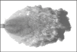
Figures 2 and 3 show the top view and side view images for a gravity current with  $\epsilon = 0.15$ ( $\gamma = 0.87$) propagating on an unbounded uniform $12\,^\circ$ slope. After the lock gate is removed, the heavy fluid in the lock collapses and spreads outward from the lock. As will be shown later, the maximum front velocity is reached at $t \approx 1.67$ s, after which the gravity current moves into the deceleration phase. The gravity current takes a wedge shape, which grows in width and height as the gravity current propagates downslope, as shown in figures 2 and 3 at $t = 2$, $8$ s. As shown in figure 2 at $t = 15$, $20$ s, an ‘active’ part of the wedge separates from the body of the current and leaves the inactive part moving slowly behind. The side view images show the edge of the ‘active’ part of the wedge is uplifted, in that the interface between the ‘active’ part of the wedge and ambient fluid is raised, in the final stage of propagation. Our observation on the separation of the ‘active’ head and mixing with the ambient fluid in the final stage of propagation is persistent for the gravity currents on an unbounded uniform $12\,^\circ$ slope at all relative density differences, including $\epsilon \approx 0.15$, $0.10$, $0.05$ ( $\gamma \approx 0.87$, $0.91$, $0.95$). Such an observation for the non-Boussinesq gravity currents is similar to the Boussinesq case (Dai & Huang Reference Dai and Huang2020), but holds a clue to the possibility that the non-Boussinesq gravity currents on an unbounded uniform $12\,^\circ$ slope may have become Boussinesq ones in the final stage of propagation, as we will discuss later. Other top view and side view images for the gravity currents at $\epsilon \approx 0.10$, $0.05$ ( $\gamma \approx 0.91$, $0.95$) are qualitatively similar and are omitted here for brevity.

Figure 2. Experiment 04/09/17-2: top view images for the gravity current on an unbounded uniform  $12\,^\circ$ slope. The reduced gravity of the heavy fluid in the lock was $g'_0 = 147.15$ cm s $^{-2}$, i.e. $\epsilon \approx 0.15$ ( $\gamma \approx 0.87$). Distances in the downslope and spanwise directions are in units of cm. Time instances are chosen at (a–d) $t=2$, $8$,
$8$,  $15$,
$15$,  $20$ s.

Figure 3. Experiment 04/09/17-2: side view images for the gravity current on an unbounded uniform  $12\,^\circ$ slope as shown in figure 2. Distances in the downslope and wall-normal directions are in units of cm. Time instances are chosen at (a–d) $t=2$, $8$,
$8$,  $15$,
$15$,  $20$ s.
4.1.2. Quantitative results
From the side view images of the gravity current, as shown in figure 3, the front location can be extracted as the furthest location reached by the gravity current and the front velocity can be calculated. Figure 4 shows the front location and front velocity histories for the gravity current at  $\epsilon \approx 0.15$ ( $\gamma \approx 0.87$) propagating on an unbounded uniform $12\,^\circ$ slope. From the front velocity history, it is observed that the gravity current moves into the deceleration phase after reaching its maximum front velocity ${U_{f}}_{max} \approx 24.38$ cm s $^{-1}$ at $t \approx 1.67$ s.

Figure 4. Experiment 04/09/17-2: front location history (a) and front velocity history (b) for the gravity current propagating on an unbounded uniform  $12\,^\circ$ slope. The reduced gravity of the heavy fluid in the lock was $g'_0 = 147.15$ cm s $^{-2}$. The maximum front velocity ${U_f}_{max} \approx 24.38$ cm s $^{-1}$ occurs at $t \approx 1.67$ s. The front location is in units of cm, front velocity is in units of cm s $^{-1}$ and time is in units of s.
To examine the front location history in the early and late stages of the deceleration phase, we plot the front location and time in terms of  ${(x_f + x_0)}^2$ vs $t$ in figure 5(a) and ${(x_f + x_0)}^{8/3}$ vs $t$ in figure 5(b). Here, $(x_f+x_0)$ represents the front location measured from the virtual origin, which can be identified by extrapolating the width of the wedge in the upslope direction, as shown in figure 1. In the early deceleration phase, the gravity current propagates downslope with an integrated wedge shape and figure 5(a) reveals that the front location history follows the power relationship (2.9) during $5 \lesssim t \lesssim 10$ s. In the late deceleration phase, an ‘active’ head separates from the body of the current and figure 5(b) reveals that the front location history follows the power relationship (2.11) during $t \gtrsim 10$ s.

Figure 5. Experiment 04/09/17-2: relationship between (a)  ${(x_f+x_0)}^2$ and $t$ and (b) ${(x_f+x_0)}^{8/3}$ and $t$ for the gravity current propagating on an unbounded uniform $12\,^\circ$ slope. The reduced gravity of the heavy fluid in the lock was $g'_0 = 147.15$ cm s $^{-2}$. The front location is in units of cm and time is in units of s. The solid line in (a) represents the straight line of best fit to the early deceleration phase and the fitting equation is ${(x_f+x_0)}^2 = {(K_I B)}^{1/2} (t+t_{I})$, where $K_I = 111.80$, $B = 117720.00$ cm $^4$ s $^{-2}$, $x_0 = 38.27$ cm and $t_I=-0.43$ s. The solid line in (b) represents the straight line of best fit to the late decelearation phase and the fitting equation is ${(x_f+x_0)}^{8/3} = K_{VS} {B}^{2/3} V^{2/9}_0 {\nu }^{-1/3} ({t+t_{VS}})$, where $K_{VS} = 3.49$ and $t_{VS}=-4.72$ s. The maximum front velocity ${U_f}_{max} \approx 24.38$ cm s $^{-1}$ occurs at $t \approx 1.67$ s.
Based on the slope of the best fit to the early deceleration phase and the buoyancy  $B=117\,720.00$ cm $^4$ s $^{-2}$, the experimental constant $K_I=111.80$ is calculated according to (2.9). The entrainment coefficient $\alpha =0.149$ is then calculated based on the experimental constant $K_I$ and (2.10). The front location history begins to deviate from the power relationship (2.9) at $t \gtrsim 10$ s, when the front Reynolds number based on the front velocity and front thickness, $Re_f=U_f h/ \nu$, is approximately $Re_f \approx 6000$. Based on the slope of the best fit to the late deceleration phase, the experimental constant $K_{VS}=3.49$ is calculated according to (2.11). Other dependent variables, including the experimental constant $K_I$, the entrainment coefficient $\alpha$ and the experimental constant $K_{VS}$, for the gravity currents propagating on unbounded uniform $12\,^\circ$, $9\,^\circ$ and $6\,^\circ$ slopes are all listed in table 2.
Table 2. Table showing the dependent variables for gravity currents propagating on unbounded uniform  $12\,^\circ$, $9\,^\circ$, $6\,^\circ$ slopes, including the entrainment coefficient $\alpha$, distance from the virtual origin to the lock gate $x_0$, experimental constant $K_{I}$, $t$ intercept $t_{I}$ in (2.9), experimental constant $K_{VS}$ and $t$ intercept $t_{VS}$ in (2.11). The subscripts $I$ and $VS$ represent the inertial phase and viscous phase on the steeper slopes in our study ( $12\,^{\circ }$, $9\,^\circ$, $6\,^\circ$), respectively. Each value is the average of five experiments. The error estimates are to add and subtract the maximum and minimum values and are not the root-mean-square estimates.

4.2. Non-Boussinesq gravity currents on unbounded uniform $9\,^\circ$ and $6\,^\circ$ slopes


Non-Boussinesq gravity currents propagating on unbounded uniform  $9\,^{\circ }$ and $6\,^{\circ }$ slopes are qualitatively similar to the non-Boussinesq gravity currents propagating on an unbounded uniform $12\,^\circ$ slope and their images are omitted for brevity. We summarise the influence of the slope angle and the relative density difference for the non-Boussinesq gravity currents on unbounded uniform $9\,^\circ$ and $6\,^\circ$ slopes and the readers are referred to tables 1 and 2 for other quantitative measures.
Figure 6 shows the experimental constant  $K_I$ against the slope angle at different values of relative density difference. In our slope angle range, based on our experiments and Ross et al. (Reference Ross, Linden and Dalziel2002), it can be concluded that the experimental constant $K_I$ increases as the slope angle increases and as the relative density difference increases. Figure 7 shows the entrainment coefficient $\alpha$ against the slope angle at different values of relative density difference. It is found that the entrainment coefficient also depends on the slope angle and decreases as the relative density difference increases, as shown in figure 7 and the inset. It is worth noting that the gravity currents propagating on unbounded uniform $12\,^\circ$, $9\,^\circ$, $6\,^\circ$ slopes maintain a wedge shape in the early deceleration phase and we may use the wedge integral model (2.10) to calculate the entrainment coefficient. As will be shown later, the gravity currents propagating on an unbounded uniform $3\,^\circ$ slope and on an unbounded horizontal boundary do not take the wedge shape and we shall not use the wedge integral model to calculate the entrainment coefficient for the gravity currents on an unbounded uniform $3\,^\circ$ slope and on an unbounded horizontal boundary.

Figure 6. Dimensionless constant  $K_I$ as a function of the slope angle $\theta$ and the relative density difference $\epsilon$. Symbols: $\square$, $\epsilon \approx 0.15$ ( $\gamma \approx 0.87$); $\circ$, $\epsilon \approx 0.10$ ( $\gamma \approx 0.91$); $\triangle$, $\epsilon \approx 0.05$ ( $\gamma \approx 0.95$); $\ast$, $\epsilon \approx 0.02$ ( $\gamma \approx 0.98$) reported by Dai & Huang (Reference Dai and Huang2020); $\blacksquare$, values reported by Ross et al. (Reference Ross, Linden and Dalziel2002), in which $0.011 \le \epsilon \le 0.039$ ( $0.962 \le \gamma \le 0.989$).

Figure 7. Entrainment coefficient  $\alpha$ as a function of the slope angle $\theta$ and the relative density difference $\epsilon$. Symbols: $\square$, $\epsilon \approx 0.15$ ( $\gamma \approx 0.87$); $\circ$, $\epsilon \approx 0.10$ ( $\gamma \approx 0.91$); $\triangle$, $\epsilon \approx 0.05$ ( $\gamma \approx 0.95$); $\ast$, $\epsilon \approx 0.02$ ( $\gamma \approx 0.98$) reported by Dai & Huang (Reference Dai and Huang2020); $\blacksquare$, values reported by Ross et al. (Reference Ross, Linden and Dalziel2002), in which $0.011 \le \epsilon \le 0.039$ ( $0.962 \le \gamma \le 0.989$); $\blacktriangledown$, values reported by Zgheib et al. (Reference Zgheib, Ooi and Balachandar2016).
As listed in table 2 and shown in figure 8, the experimental constant  $K_{VS}$ increases as the slope angle increases but, surprisingly, appears not to be strongly influenced by the relative density difference. As shown in figure 8, for $0.05 \le \epsilon \le 0.15$, $K_{VS}$ varies erratically in the range $3.49 \le K_{VS} \le 4.66$ at $\theta =12^\circ$, $3.05 \le K_{VS} \le 4.24$ at $\theta =9^\circ$ and $2.25 \le K_{VS} \le 3.26$ at $\theta =6^\circ$. The fact that the influence of the relative density difference on $K_{VS}$ is not significant suggests that the non-Boussinesq gravity currents on unbounded uniform $12\,^\circ$, $9\,^\circ$ and $6\,^\circ$ slopes may have become Boussinesq ones in the late deceleration phase.

Figure 8. Dimensionless constant  $K_{VS}$ as a function of the slope angle $\theta$. The influence of the relative density difference on $K_{VS}$ is not significant in the range $0.05 \le \epsilon \le 0.15$. Symbols: $\square$, $\epsilon \approx 0.15$ ( $\gamma \approx 0.87$); $\circ$, $\epsilon \approx 0.10$ ( $\gamma \approx 0.91$); $\triangle$, $\epsilon \approx 0.05$ ( $\gamma \approx 0.95$).
4.3. Non-Boussinesq gravity currents on an unbounded uniform $3\,^\circ$ slope

Non-Boussinesq gravity currents propagating on an unbounded uniform  $3\,^\circ$ slope are qualitatively different from the non-Boussinesq gravity currents on unbounded uniform $12\,^\circ$, $9\,^\circ$ and $6\,^\circ$ slopes. The gravity current maintains a shape more akin to a disk even in the late deceleration phase, as shown by the top view and side view images in figures 9 and 10.

Figure 9. Experiment 07/26/17-2: top view images of the gravity current propagating on an unbounded uniform  $3\,^\circ$ slope. The reduced gravity of the heavy fluid in the lock was $g'_0 = 147.15$ cm s $^{-2}$, i.e. $\epsilon \approx 0.15$ ( $\gamma \approx 0.87$). Distances in the downslope and spanwise directions are in units of cm. Time instances are chosen at (a–d) $t=6$, $10$,
$10$,  $15$,
$15$,  $20$ s. In this experiment, the maximum front velocity ${U_f}_{max} \approx 18.00$ cm s $^{-1}$ occurs at $t \approx 1.67$ s.

Figure 10. Experiment 07/26/17-2: side view images for the gravity current propagating on an unbounded uniform  $3\,^\circ$ slope as shown in figure 9. Distances in the downslope and wall-normal directions are in units of cm. Time instances are chosen at (a–d) $t=6$, $10$,
$10$,  $15$,
$15$,  $20$ s.
In the early deceleration phase, figure 11(a) shows that the front location history follows the power relationship (2.9) during  $5 \lesssim t \lesssim 15$ s and we may calculate the experimental constant $K_I=26.70$, which is listed in table 3. At $t \gtrsim 15$ s, the front location history begins to deviate from the power relationship (2.9) when the front Reynolds number is approximately $Re_f \approx 2000$. In the late deceleration phase, figure 11(b) shows that the front location history follows the power relationship (2.12) during $t \gtrsim 15$ s and we may calculate the experimental constant $K_{VM}=94.37$, which is also listed in table 3. The experimental constant $K_{VM}$ is evidently not only a function of the slope angle but also a function of the relative density difference. The influence of the relative density difference is carried along into $K_I$ during the early deceleration phase and into $K_{VM}$ during the late deceleration phase for the gravity currents on an unbounded uniform $3\,^\circ$ slope.

Figure 11. Experiment 07/26/17-2: relationship between (a)  ${(x_f+x_0)}^2$ and $t$ and (b) ${(x_f+x_0)}^{4}$ and $t$ for the gravity current propagating on an unbounded uniform $3\,^\circ$ slope. The reduced gravity of the heavy fluid in the lock was $g'_0 = 146.87$ cm s $^{-2}$. The front location is in units of cm and time is in units of s. The solid line in (a) represents the straight line of best fit to the early deceleration phase and the fitting equation is ${(x_f+x_0)}^2={(K_I B)}^{1/2} (t+t_{I})$, where $K_I = 26.70$, $B = 117\,720.00$ cm $^4$ s $^{-2}$, $x_0 = 13.15$ cm and $t_I=-1.05$ s. The solid line in (b) represents the straight line of best fit to the late deceleration phase and the fitting equation is ${(x_f+x_0)}^{4} = K_{VM} {B}^{2/3} V^{2/3}_0 {\nu }^{-1/3} ({t+t_{VM}})$, where $K_{VM}=94.37$ and $t_{VM}= -8.67$ s. The maximum front velocity ${U_f}_{max} \approx 18.00$ cm s $^{-1}$ occurs at $t \approx 1.67$ s.
Table 3. Table showing the dependent variables for gravity currents propagating on a  $3\,^\circ$ unbounded uniform slope and on an unbounded horizontal boundary, including the distance from the virtual origin to the lock gate $x_0$, experimental constants $K_{I}$, $t$ intercept $t_{I}$ in (2.9), experimental constant $K_{VM}$ and $t$ intercept $t_{VM}$ in (2.12). The subscripts $I$ and $VM$ represent the inertial phase and viscous phase on the milder slopes in our study ( $3\,^\circ$ and $0\,^{\circ }$), respectively. Each value is the average of five experiments. The error estimates are to add and subtract the maximum and minimum values and are not the root-mean-square estimates.

4.4. Non-Boussinesq gravity currents on an unbounded horizontal boundary
We also performed the experiments on the gravity currents on an unbounded horizontal boundary, of which the morphology (not shown) is qualitatively similar to the gravity current on an unbounded uniform  $3\,^\circ$ slope.
For the gravity currents on an unbounded horizontal boundary, the experimental constant  $K_I$ tends to increase as the relative density difference increases, as shown in table 3. In the late deceleration phase, the experimental constant $K_{VM}$ is a function of both the slope angle and the relative density difference, as listed in table 3 and shown in figure 12. The influence of the relative density difference is carried along into the late deceleration phase on $K_{VM}$ for the gravity currents on an unbounded horizontal boundary. Our observations suggest that the non-Boussinesq gravity currents on an unbounded uniform $3\,^\circ$ slope and on an unbounded horizontal boundary may still remain non-Boussinesq ones in the late deceleration phase.

Figure 12. Dimensionless constant  $K_{VM}$ as a function of the slope angle $\theta$ and the relative density difference $\epsilon$. The influence of the relative density difference on $K_{VM}$ is clear, as also shown in table 3. Symbols: $\square$, $\epsilon \approx 0.15$ ( $\gamma \approx 0.87$); $\circ$, $\epsilon \approx 0.10$ ( $\gamma \approx 0.91$); $\triangle$, $\epsilon \approx 0.05$ ( $\gamma \approx 0.95$).
5. Conclusions
Experiments on the Boussinesq and non-Boussinesq gravity currents produced from a finite volume of heavy fluid propagating into an environment of light ambient fluid on unbounded uniform slopes in the range  $0\,^{\circ } \le \theta \le 12^{\circ }$ are presented. The relative density difference covers the Boussinesq and non-Boussinesq cases in the range $0.05 \le \epsilon \le 0.15$ in this study. After the lock gate is removed, the gravity currents go through an acceleration phase and move into the early and late stages of the deceleration phase. Our focus in this study is on the influence of the relative density difference on the deceleration phase of the propagation.
For the gravity currents propagating on unbounded uniform  $12\,^\circ$, $9\,^\circ$ and $6\,^\circ$ slopes, in the early deceleration phase, the gravity currents take a wedge shape and the front location history follows the power relationship (2.9), in which the dimensionless constant $K_I$ is a function of both the slope angle and the relative density difference. In the late deceleration phase, an ‘active’ head separates from the body of the current and mixes with the ambient fluid. The front location history in the late deceleration phase follows the power relationship (2.11), in which the dimensionless constant $K_{VS}$ is influenced by the slope angle but not significantly influenced by the relative density difference. The observation that the relative density difference has no significant influence on the dimensionless constant $K_{VS}$ in the late deceleration phase suggests that the non-Boussinesq gravity currents on unbounded uniform $12\,^\circ$, $9\,^\circ$ and $6\,^\circ$ slopes may have become Boussinesq ones in the late deceleration phase.
For the gravity currents propagating on an unbounded uniform  $3\,^\circ$ slope and on an unbounded horizontal boundary, the gravity currents maintain an integrated disk shape throughout the motion. In the early deceleration phase, the front location history follows the power relationship (2.9) and the dimensionless constant $K_I$ is a function of both the slope angle and the relative density difference. In the late deceleration phase, the gravity currents still maintain an integrated disk shape without the separation of an ‘active’ head from the body of the gravity currents. The front location history in the late deceleration phase follows the power relationship (2.12), in which the dimensionless constant $K_{VM}$ is influenced by both the slope angle and the relative density difference. The influence of the relative density difference is carried along into the late deceleration phase on $K_{VM}$ and such an observation suggests that the non-Boussinesq gravity currents on an unbounded uniform $3\,^\circ$ slope and on an unbounded uniform horizontal boundary may still remain non-Boussinesq ones in the late deceleration phase.
Our experiments indicate that, depending on the slope angle, two different flow morphologies are possible concerning the final stage of the non-Boussinesq gravity currents propagating on unbounded uniform slopes. More importantly, our results further indicate that the non-Boussinesq gravity currents on the milder unbounded uniform slopes in this study ( $3\,^\circ$ and $0\,^\circ$) may remain non-Boussinesq ones in the late deceleration phase while the non-Boussinesq gravity currents on the steeper unbounded uniform slopes in this study ( $12\,^\circ$, $9\,^\circ$ and $6\,^\circ$) may have become Boussinesq ones in the late deceleration phase. The above findings on the basis of dimensional arguments are in accordance with our observation that the mixing for the gravity currents on the steeper unbounded uniform slopes in the late deceleration phase is more violent than the mixing for the gravity currents on the milder unbounded uniform slopes in the late deceleration phase.
Acknowledgements
A. D. is grateful for encouragement from Professors P. Linden and S. Dalziel at the University of Cambridge, S. Balachandar at the University of Florida, M. Garcia and G. Parker at the University of Illinois at Urbana-Champaign. Funding supports from Taiwan Ministry of Science and Technology through grant MOST-109-2628-E-002-006-MY2 and from National Taiwan University through grant 109L7830 are greatly acknowledged.
Declaration of interests
The authors report no conflict of interest.


 Open access