


Broadberry, Guan, and Li (2018; hereinafter BGL) have estimated China’s GDP back to 980, farther back than any recent work on European economies. Although there are gaps, their decadal estimates cover large parts of the Song, Ming, and Qing dynasties. BGL argue that their work makes it clear that the Great Divergence in per capita incomes between northwest Europe and China dates from the early eighteenth century. Unfortunately, a serious error in their estimates for the government sector renders the estimates and the conclusions drawn from them invalid. This comment revises the government sector to produce more plausible GDP estimates and shows that divergence may date from much earlier. It also briefly assesses the nature and coverage of the data underlying BGL’s estimates for other sectors and suggests an agenda for further research. Concerns about the quality of the data underlying estimates for other sectors will be left to the China specialists (see, e.g., Deng and O’Brien Reference Deng and O’Brien2016).
The problem with BGL’s government sector series is immediately evident when expressed either as government expenditure per capita or as a share of their GDP estimates (Figure 1). Government spending per capita is more than seven times higher in the early Ming than in the mid-nineteenth century. The government share in GDP rises to over 35 percent in the early Ming and remains at more than 15 percent from the late Song to the early Qing.Footnote 1 By the standard of pre-industrial economies, these shares are implausibly high. In Europe, peace-time government spending before the twentieth century rarely exceeded 10 percent (Prados de la Escosura 2007, p. 203; Bogart et al. Reference Bogart, Drelichman, Gelderblom, Rosenthal, Broadberry and O’Rourke2010). In India, Broadberry, Custodis, and Gupta’s (Reference Broadberry, Custodis and Gupta2015) estimates for the government share never exceed 2.7 percent between 1600 and 1840.
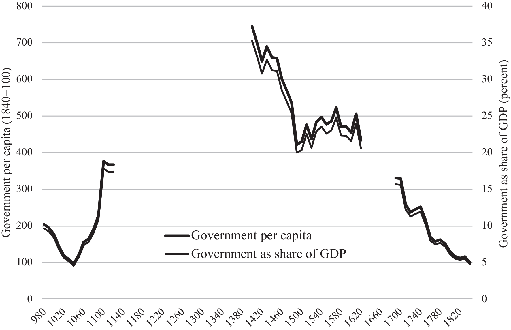
Figure 1 GOVERNMENT PER CAPITA AND AS A SHARE OF GDP
Notes: Steve Broadberry kindly supplied the indices that underlie the figures in the paper, which were not in the replication file.
Source: Broadberry, Guan, and Li (2018).
BGL’s shares for government expenditure are also inconsistent with evidence on government shares of expenditure or taxes in pre-industrial China. Deng (Reference Deng, Yun-Casalilla and O’Brien2012) reckons that under the Qing, the state may have controlled only some 8 percent of GDP, and Ma (Reference Ma2013) shows how the Qing state’s revenue per capita was small by international standards. For the late sixteenth century, when BGL’s government share is still over 20 percent, Huang (Reference Huang1975, pp. 166–70) has calculated the share of the land tax in agricultural output as 6.7 percent in Hangzhou prefecture on the east coast and 5 percent in Fenzhou prefecture in the north. Since taxes on agriculture constituted the bulk of imperial revenue during the Ming (Wong Reference Wong, Yun-Casallia and O’Brien2012), these figures must mean that the overall tax burden could not have exceeded 10 percent. Some back-of-the-envelope calculations by Feuerwerker (Reference Feuerwerker1984) put the government share under the Song at a relatively high 13 percent, but only 6–8 percent under the Ming and 4–8 percent in the early Qing. These much smaller government shares underpin Rosenthal and Wong’s (2011) argument that because China faced fewer military threats, the size of its government sector was always relatively small.
What may have gone wrong with BGL’s estimates for the government sector? The estimates are based on numbers employed in the civil service and the military multiplied by their salaries, with the resulting figures for nominal expenditure deflated by the prices of grain and cloth.Footnote 2 The military far outnumbered the civil service, with figures for the size of the army at the beginning of the Ming in the range of 1.3–1.8 million soldiers (Swope Reference Swope2009). In a population of 70 million at the time, the adult male labor force would have been about 14 million, implying, at first pass, that the government share was no more than 10–15 percent.Footnote 3 For the government share of GDP to have been over 30 percent, average incomes in the public sector would have to have been at least two and a half times higher than in the rest of the economy. But soldiers were said to have been paid at the rate of day laborers (Robinson Reference Robinson and Zürcher2013), which suggests problems with either the salaries or the prices used by BGL.
A closer look at what soldiers did also raise the possibility of considerable double-counting in the early Ming and possibly in other periods as well. Much, if not most, of soldiers’ time was spent growing their own food; others, perhaps as many as 100,000, were occupied in transporting grain by the Grand Canal (Robinson Reference Robinson and Zürcher2013). Military land accounted for 3–5 percent of all cultivated land in the early Qing and probably more during the Ming (Shi Reference Shi2020, pp. 26, 44, 48). The estimates for agriculture and the transport of agricultural goods, both based on the cultivated land area and grain yields, incorporate no adjustment for such activity by the military. The numbers in the public sector may also have been inflated by the inclusion of corvée labor for handicraft production, which was prevalent particularly during the early Ming (Wen-Chin Reference Wen-Chin1988).Footnote 4 The estimates for industry, based as they are on population and urbanization, would not correct for changes in the extent of industrial activity within the government sector.
Does BGL’s implausibly large government sector make a difference to our understanding of the pattern of economic change in pre-industrial China? Revised estimates can be made on three alternative assumptions about the government sector: (1) that it grew in line with population; (2) that its share of GDP remained constant over the entire period at its 1840 level; and (3) that its share of GDP followed Feuerwerker’s rough estimates (Song, 13 percent; Ming, 7 percent; Qing, 6 percent). On the first assumption, the alternative estimate for GDP has been made by substituting BGL’s index of population for their index of government expenditure and recalculating GDP using BGL’s indices for other sectors. On the second and third assumptions, total output in the rest of the economy has been recalculated without BGL’s government series, then these figures have been inflated by the assumed government share to arrive at alternative series for GDP.
Figure 2 shows the series for Chinese GDP per capita recalculated on these three assumptions and compares them to BGL’s estimates (Reference SolarSolar 2021). The first thing to note is that the three assumptions give essentially the same results, except that during the Song when Feuerwerker’s higher government share leads to higher per capita GDP and the population-based series to lower per capita GDP. The second is that such assumptions sacrifice the temporal detail of annual, or even decadal, returns of government revenue or expenditure. The Chinese government’s spending depended heavily on whether it had to fight off invaders, quell civil disturbances, or confront rival warlords (Ma Reference Ma2013). But estimates based on such simple assumptions may be sufficient and more appropriate for long-run comparisons of peacetime national income.

Figure 2 GDP PER CAPITA: ORIGINAL AND REVISED GOVERNMENT SECTOR (1840 = 100)
Notes: The revised figures reflect the replacement of the original government sector series by three series created on different assumptions: (1) that the government share of GDP remained constant at its 1840 value throughout; (2) that the government share of GDP followed Feuerwerker’s calculations: 13 percent during the Song; 7 percent during the Ming; 6 percent during the Qing; (3) that the government sector maintained a constant relationship with population.
Source: Broadberry, Guan, and Li (2018).
When compared to BGL’s estimates, the revised estimates leave the Song peak largely unchanged, except, again, where Feuerwerker’s higher government share makes it even more pronounced. The major change occurs during the Ming, when the revised estimates are 25 percent lower early in the period, falling to about 15 percent lower in the late Ming.Footnote 5 These changes restore the Song efflorescence to its prominent place in global history, whereas on BGL’s estimates of per capita incomes, the Song peak had been equaled, if not slightly surpassed, in the early Ming. The revised estimates also show per capita incomes not to have changed very much during the Ming.
The revised estimates highlight a sharp peak in Chinese GDP per capita c.1700. Xu et al.’s (Reference Xu, Zhihong, van Leeuwen, Ni, Zhang and Ma2015, Reference Xu, Zhihong, van Leeuwen, Ni, Zhang and Ma2017) estimates for GDP per capita begin in 1660 and fall from then onwards; in the early eighteenth century, at more or less the same pace as the revised BGL estimates. Their work suggests that the peak, sometime in the mid-seventeenth century, was even higher and the corresponding rise in per capita income from the Ming even larger. Real wage evidence, while not the same as GDP per capita, indicates that such a peak may have occurred in the 1660s: a sharp rise in real wages, amounting to an astonishing 150 percent, has been estimated to have taken place from the 1640s to the 1660s, though this was a particularly troubled period (de Zwart and van Zanden 2018, p. 218).
How do the revisions affect international comparisons? We will use our revised estimates to investigate this, but first, BGL’s 1840 benchmark for Chinese GDP per capita (599 1990 dollars) needs revision as well. Although they claim to have data for nominal GDP in 1840, their figures are based on the extrapolation, using only a series for grain output, of 1880s GDP back to 1840, with the remaining sectors being estimated according to their shares in the 1880s. Other scholars have made more direct estimates of Chinese GDP back to the mid-nineteenth century. Xu et al. (Reference Xu, Zhihong, van Leeuwen, Ni, Zhang and Ma2015, Reference Xu, Zhihong, van Leeuwen, Ni, Zhang and Ma2017) put GDP per capita in 1850 at 538, also in 1990 dollars. Ma and de Jong (2019) come up with $528 in 1840 and $532 in 1850. The latter’s annual estimates show GDP per capita to be essentially flat during the 1840s, so, taking the results of these alternative estimates together, Chinese GDP per capita in 1840 might be set at $535, about 11 percent lower than BGL’s figure.
Revised estimates for Chinese GDP per capita, on the assumption of a constant government share at its 1840 level, are shown, along with figures for Italy, the Netherlands, and Great Britain, in Table 1, an abbreviated version of BGL’s Table 8. These show that levels of GDP per capita in the European leaders were well above those in China from at least 1400 when figures for all four countries are first available. But, as the California school has rightly insisted, the appropriate comparison is with China’s leading region, the Yangzi delta. BGL (p. 990) take, as an upper bound, that per capita incomes in the delta were 75 percent higher than those for China as a whole.Footnote 6 Adopting this assumption and comparing the Yangzi delta to the leading European country at each date produces Figure 3, a revised version of BGL’s Figure 8.
Table 1 GDP PER CAPITA LEVELS IN EUROPE AND ASIA (1990 International Dollars)

Sources: China: Appendix Table 1; Italy, Netherlands, and Great Britain: Broadberry, Guan, and Li (2018).
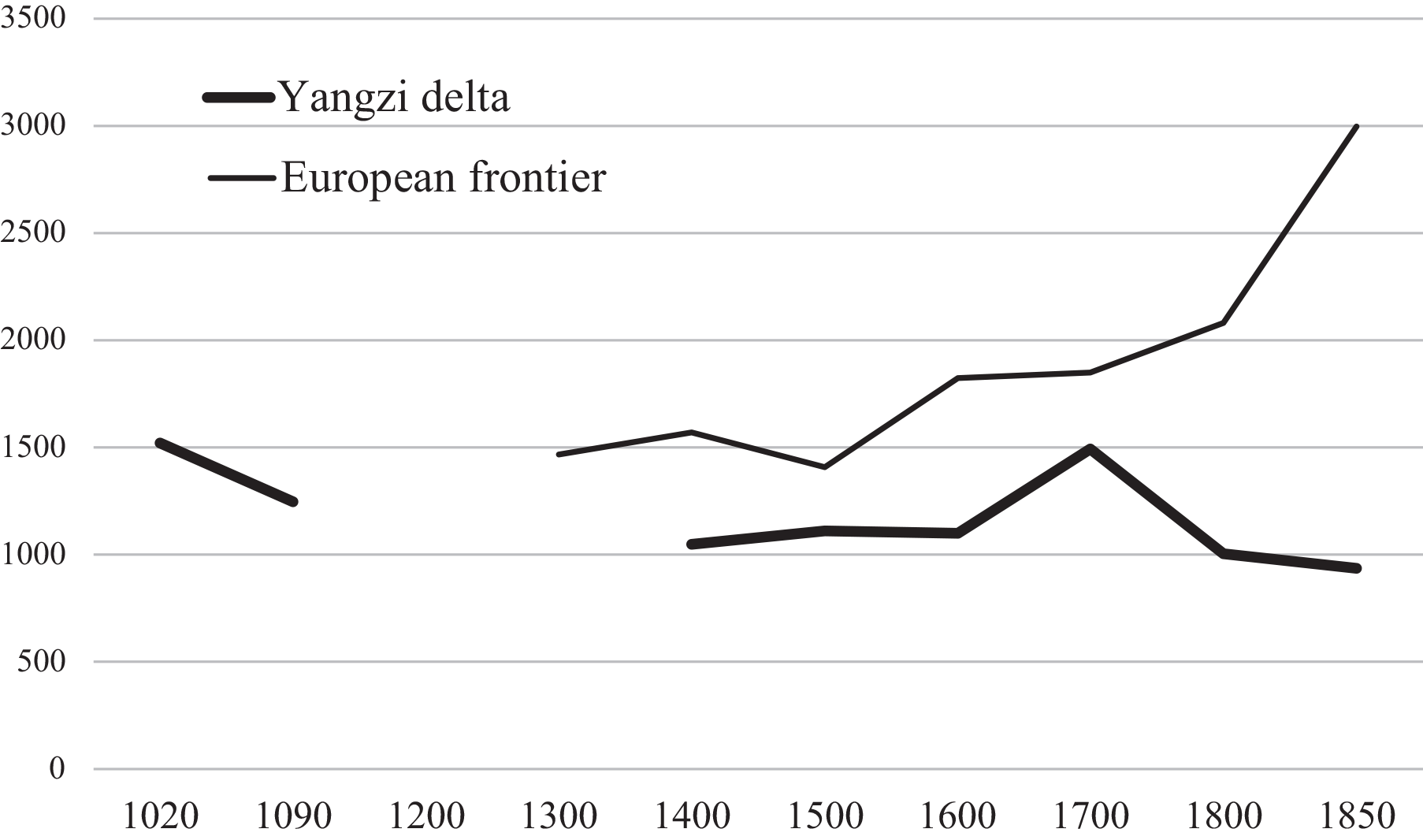
Figure 3 GDP PER CAPITA IN THE LEADING REGIONS OF EUROPE AND CHINA, 1020–1850 (1990 International Dollars)
Notes: European frontier: maximum of Italy, Netherlands, and Great Britain; Yangzi Delta: 1.75 times China, which is the series constructed on the assumption that the government share remained constant at its 1840 value.
Source: Table 1.
The picture of development in China relative to Europe looks very different from that given by BGL. Their estimates showed per capita income levels in the Yangzi delta as more or less equivalent to those in the leading European countries from 1400 until 1700, after which there was a very sharp divergence. The revised figures show, by contrast, that during the Ming, per capita incomes in the delta were 20–40 percent lower than in the European leader, and these comparisons are based on BGL’s upper bound estimates.
BGL do not make international comparisons before 1400 for want both of estimates before 1300 for Italy, the leading European country, and of estimates for China in 1300. But the high level of income per capita in the Song does suggest that there may have been a Great Crossing in the Middle Ages. As per capita incomes fell in China during the late Song and between the Song and the Ming, they probably rose in Italy, the leading European country. Trends in urbanization support this hypothesis. Malanima (Reference Malanima2005) suggests that the urbanization rate in Italy at least doubled between 1000 and 1300. By contrast, Xu ,van Leeuwen, and van Zanden (Reference Xu, van Leeuwen and van Zanden2018) see the urbanization rate in the Yangzi delta falling from 25 to 18 percent during the thirteenth century, and this was a century or more after the Song peak in the eleventh century. A crossing in the Middle Ages is also consistent with trends in manuscript and book production which Buringh and van Zanden (2009) and Chaney (Reference Chaney2018) have taken as indicators of development.
BGL’s original estimates, and the revised estimates even more so, pose a major problem for the dating of the Great Divergence. According to the revised estimates, per capita incomes in the Ming were not much different from those in the mid-eighteenth century, but in the interim, there was a major peak in per capita income c.1700. As noted above, on Xu et al.’s (Reference Xu, Zhihong, van Leeuwen, Ni, Zhang and Ma2017) estimates, this peak may have been even higher and situated somewhat earlier, in the second half of the seventeenth century. In the international comparisons the result is, to multiply the Greats, a Great Convergence in the seventeenth century, then a Greater Divergence during the eighteenth and early nineteenth centuries. Without this peak, a more gradual divergence between the Yangzi delta and the European leaders may have started as early as the fifteenth or sixteenth century. Was this peak real? Did per capita incomes rise by almost a quarter from the late Ming to the early Qing and reach a level comparable to that in the Song efflorescence?
The central feature of China’s seventeenth-century history is the dynastic change from the Ming to the Qing, which was marked by famine and war. Figures cited for population losses, often covering different periods, are on the order of about a fifth (Marks Reference Marks1998, p. 158; Myers and Wang Reference Myers, Wang and Willard2002, pp. 565, 571; Shi Reference Shi2020, p. 179). After the Black Death in Europe, the population decline led to an increase in the relative price of labor. In the mid-seventeenth century, Chinese rice prices doubled, but land prices remained largely unchanged, suggesting a similar change in relative prices (von Glahn Reference von Glahn1996). This should have resulted in less intensive cultivation, which would not necessarily be captured when agricultural output is estimated only as grain yields times the entire cultivated area. The Chinese economy was also disrupted by a ban on maritime trade from 1661 to 1683 and continuing wars to consolidate the regime. The period from 1660 to 1690 has been described as the “Kangxi depression,” which does not suggest a period in which per capita incomes were exceptionally high (von Glahn Reference von Glahn2016). In the qualitative literature, at least in English, the subsequent decades are seen as a period of recovery, not as one of singular prosperity (Myers and Wang Reference Myers, Wang and Willard2002; Rowe and Brook Reference Rowe and Brook2009; von Glahn Reference von Glahn2016). Yet, on the revised estimates, when the Chinese population had recovered its late Ming level in the first decades of the eighteenth century, per capita incomes were 20–25 percent higher.
This late seventeenth-century or early eighteenth-century peak might, at least in part, be due to BGL’s figures for China’s population in 1700 being too low. The seventeenth century is a notably uncertain period for estimates of population. Deng (Reference Deng2004) argues vigorously for sticking to the official counts, but most authors either adjust these counts upwards by at least twofold or they extrapolate forward from the late fourteenth century or backward from the late eighteenth century when population figures are regarded as somewhat more reliable.Footnote 7 Table 2 and Figure 4 show various estimates for China’s population in the seventeenth and eighteenth centuries, including indications of where extrapolations have been made. Although BGL state that “there seems to be a high degree of consensus about the trend of China’s population over this period” (p. 964), when their estimate c.1700 is compared with other recent work, it is clearly at the lower end, mainly because their extrapolation backward from 1750 has been made at a particularly steep rate, implying population growth at 1.27 percent per capita over the entire first half of the eighteenth century. Implicitly, BGL are assuming that population growth was slow in the second half of the seventeenth century, probably less than half a percent, before accelerating sharply around 1700 and subsequently decelerating, equally sharply, to 0.55 percent after 1750. By contrast, Xu et al. (Reference Xu, Zhihong, van Leeuwen, Ni, Zhang and Ma2017) assume that growth was constant over the late seventeenth and early eighteenth centuries, Shi (Reference Shi2020) that there was a modest acceleration from the 1720s and Cau (2000) that growth was accelerating throughout the period. This is hardly “a high degree of consensus.” Adopting any of the higher estimates for the Chinese population c.1700 would reduce the peak in Chinese GDP per capita shown in both BGL’s original and revised estimates; using Cao’s figure would eliminate it entirely, leaving per capita GDP at more or less the same level as in 1620.
Table 2 CHINESE POPULATION LEVELS (Million)
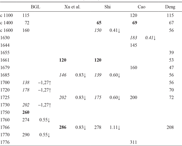
Notes: Shuo Chen kindly supplied me with the data from Cao. Numbers in italics are extrapolations or interpolations from the values in bold; arrows show the direction of extrapolation.
Sources: BGL: Broadberry, Guan, and Li (2018); Xu et al. (Reference Xu, Zhihong, van Leeuwen, Ni, Zhang and Ma2017); Shi (Reference Shi2020); Cao (Reference Cao2000); Deng (Reference Deng2004).

All of these conclusions depend on the accuracy of BGL’s estimates of Chinese GDP as revised. Even with a more plausible government sector, BGL’s estimates for China’s historical GDP can only be a first, relatively limited, sketch for a fuller picture of how the country’s economy evolved in the past. Table 3 unravels how the various subsectors have been estimated, rearranging them to show how much the GDP estimates depend on each of the data series that underlies them. For example, the series for salt, iron, and copper outputs were first used to estimate the output of other metals and then, along with other industrial sectors, used to estimate the share of commercial services (transport, trade, and finance) relating to industrial output. “Grain output” (total cultivated area times cereal yield) stands in for the rest of commercial services, as well as for the food processing industry, agricultural output other than grain, and fishing and forestry.
Table 3 WEIGHTS OF UNDERLYING SERIES IN THE GDP ESTIMATES, 1840

Notes: “Grain output” = total cultivated area x rice and wheat yields. Note that the figures for commerce, government, and housing and other private services in Broadberry, Guan, and Li’s Table 2 are incorrect; they should be 503,932, 254,823, and 629,654, respectively.
Source: Broadberry, Guan, and Li (2018).
What is striking about Table 3 is that, ultimately, the estimates of Chinese GDP over the long term depend, for over 92 percent, on “grain output” and population, the latter sometimes adjusted by urbanization.Footnote 8 Since most economies before the twentieth century were poor and predominantly agricultural, such heavy reliance on grain output might indeed be a first approximation to the size of the economy. But it may not always be a very good approximation. Consider the case of England, drawing on the data underlying Broadberry et al.’s (Reference Broadberry, Custodis and Gupta2015) estimates. Series for English agricultural output, calculated, as for China, as the yield of wheat times the entire cultivated area, and for English population move so much in synch that, no matter what the weighting scheme, estimates of English GDP per capita based on just these two series show it to have remained essentially constant over six centuries. By contrast, Broadberry et al.’s more sophisticated estimates show English GDP per capita to have tripled over this period, in part because of structural changes both within the agricultural sector and between it and the industrial and service sectors.Footnote 9
Table 3 suggests that, as things stand, the top priority for historical national accounts should be to make sure that the series for population and “grain output” be as accurate as possible. Although Deng and O’Brien (Reference Deng and O’Brien2016) have cast doubt on the possibility of making sense of the multitude of land area measures in use, Shi (Reference Shi2020) has tried to do so.Footnote 10 As noted previously, Deng (Reference Deng2004) has criticized the population figures, and Table 2 and Figure 4 show the uncertainties of extrapolation over even relatively short periods. Since agriculture was throughout the millennium the major sector of the Chinese economy, a second priority would be to understand how changes in specialization within that sector may have influenced overall output. “Grain output” has been put in quotations because agricultural output has been estimated by multiplying the total cultivated area by an amalgam of rice and wheat yields. How was the value of agricultural output influenced by increasing or decreasing cultivation of other crops, such as tea, silk, or cotton, all of which produced more value per area? Or by the introduction of new crops such as maize and sweet potatoes? A third priority would be better indicators of the movements in industrial output. As it stands, industrial output is essentially estimated from the level of population and the output of salt.Footnote 11 What can be said about trends in important industries like silk, cotton, and ceramics? Qualitative evidence on new goods and services and specialization and trade, in the Chinese case mainly internal trade, are important for understanding potential biases in GDP estimates. Kelly (Reference Kelly1997) has argued, for example, that the Song efflorescence was an example of Smithian growth as the development of a national waterway network led to the creation of a national market with increased regional specialization. Given the problems noted earlier with the government sector, a fourth priority would be better series for government expenditure or revenue. It may not be possible, indeed it is likely to be impossible to construct long quantitative series for all of these elements. Hence there is a need for historical national accountants to give users of their statistics a clear, albeit qualitative, idea of how and when their estimates may be overstating or understating changes in output.


